Lambda-Nucleon and Sigma-Nucleon potentials from space-time correlation function on the lattice

Abstract

The hyperon-nucleon interaction with the strangeness $S=-1$ region is complicated and difficult to investigate because its flavor sector involves all the irreducible representation except the flavor singlet and has the worst signal-to-noise ratio among the strangeness regions. In order to overcome such difficulties the content of this report is twofold: (i) We present an implementation of extended effective baryon block algorithm. This is a straightforward extension of the original which was reported in LATTICE 2013. (ii) We perform single channel analysis for the $\Lambda N$ system at nearly physical quark masses corresponding to $(m_{\pi},m_{K})\approx(146,525)$ MeV and large volume $(La)^{4}=(96a)^{4}\approx$ (8.1 fm)⁴. Scattering phase shifts for $\Lambda N$ system are presented.

1 Introduction

Atomic nucleus is a finite quantum many-body system of nucleons bound by the strong interaction (nuclear force). In the low energy region, nuclear phenomena have been studied with much success by assuming that the nucleon is the fundamental degree of freedom. On the other hand, in systems including strangeness, the hyperonic nuclear forces have still large ambiguities because of the lack of sufficient experimental data. Neutron stars with twice the solar mass have been observed[1, 2, 3], and an accurate understanding of the hyperonic nuclear force is a major issue in understanding the structure of dense nuclear states such as those near the core of neutron stars.

Comprehensive study of generalized baryon-baryon ($BB$) interaction with containing strangeness is one of the important subject. HAL QCD method[4] is one of the fascinating approaches. In order to calculate a wide range of $BB$ interactions simultaneously, we had presented the effective baryon block algorithm in LATTICE 2013[5]. Since this algorithm does not impose any restrictions on the quark fields on each baryon in the source, there is no need for each quark field in the source to be spatially identical between the baryons. The Wick contraction can be performed appropriately no matter what quantum state is considered.

The coupled-channel potentials of $\Lambda N-\Sigma N$ system at nearly physical quark masses corresponding to $(m_{\pi},m_{K})=(146,525)$ MeV with large volume $(La)^{4}=(96a)^{4}=(8.1~{}\mathrm{fm})^{4}$ had been reported in LATTICE 2017[6]. The $\Sigma N-\Sigma N$ potential in the ${}^{1}S_{0}$ channel has large statistical noise which impedes further analysis.

The purpose of this report is twofold: (i) We present an implementation of extended effective baryon block algorithm. It is straightforward from the first implementation [7] since the original algorithm does not impose any restrictions on the quark fields on each baryon in the source. (ii) We present single channel analysis for the $\Lambda N$ system at nearly physical quark masses corresponding to $(m_{\pi},m_{K})=(146,525)$ MeV with large volume $(La)^{4}=(96a)^{4}=(8.1~{}\mathrm{fm})^{4}$. By employing the single-channel analysis the statistical uncertainty of the single channel $\Lambda N$ potential is reduced. We can derive the scattering phase shifts below the $\Sigma N$ threshold by employing an analytical functional form for representing the lattice (discretized) potential.

2 HAL QCD method with effective baryon block algorithm

The baseline quantity for studying the $\Lambda N$ interaction with the HAL QCD method is the four-point correlation function (4pt-correlator) in the center-of-mass frame,

$${F}_{\alpha_{1}\alpha_{2},\alpha_{3}\alpha_{4}}^{\langle p\Lambda\overline{p\Lambda}\rangle}(\vec{r},t-t_{0})=\sum_{\vec{X}}\left\langle 0\left|p_{{\alpha_{1}}}(\vec{X}+\vec{r},t)\Lambda_{{\alpha_{2}}}(\vec{X},t)\overline{{\cal J}_{p_{\alpha_{3}}\Lambda_{\alpha_{4}}}(t_{0})}\right|0\right\rangle.$$ (1)

The $p$ and $\Lambda$ denote the interpolating fields of proton and $\Lambda$ which comprise up, down and strange quark fields, $u$, $d$, $s$,

$$\!\!\!\begin{array}[]{llll}p\!=\!X_{\mathrm{udu}},\!&\Lambda\!=\!{1\over\sqrt{6}}\left(X_{\mathrm{dsu}}\!+\!X_{\mathrm{sud}}\!-\!2X_{\mathrm{uds}}\right),\!&\mathrm{with}~{}X_{\mathrm{fgh}}\!=\!\varepsilon_{abc}\!\left(\mathrm{f}_{a}C\gamma_{5}\mathrm{g}_{b}\right)\!\mathrm{h}_{c},&(\mathrm{f},\mathrm{g},\mathrm{h})\!\in\!\left\{u,d,s\right\}.\end{array}$$ (2)

The 4pt-correlator is evaluated through the effective baryon block algorithm [7, 8] together with Fast Fourier Transform (FFT). For simplicity, we show only the contributions from $\overline{X}_{\mathrm{dsu}}$ in the $\overline{\Lambda}$ in the source.

$${F}^{\langle p\Lambda\overline{pX_{\mathrm{dsu}}}\rangle}_{{\alpha_{1}}{\alpha_{2}},{\alpha_{3}}{\alpha_{4}}}(\vec{r})=\sum_{\vec{X}}\left\langle 0\left|p_{{\alpha_{1}}}(\vec{X}+\vec{r},t)\Lambda_{{\alpha_{2}}}(\vec{X},t)\overline{{\cal J}_{p_{\alpha_{3}}X_{\mathrm{dsu},\alpha_{4}}}(t_{0})}\right|0\right\rangle,$$ (3)

$$= {1\over L^{3}}\sum_{\vec{q}}\left([\widetilde{p}_{\alpha_{1}\alpha_{3}}^{(1)}](\vec{q})[\widetilde{\Lambda}_{\alpha_{2}\alpha_{4}}^{(1)}](-\vec{q})-[\widetilde{p}_{\alpha_{1}\alpha_{4}}^{(2)}]_{c_{3}^{\prime},c_{6}^{\prime}}(\vec{q})[\widetilde{\Lambda}_{\alpha_{2}\alpha_{3}}^{(2)}]_{c_{3}^{\prime},c_{6}^{\prime}}(-\vec{q})\right.$$

$$\left.-[\widetilde{p}_{\alpha_{1}\alpha_{3}}^{(3)}]_{c_{2}^{\prime},\alpha_{2}^{\prime},c_{4}^{\prime},\alpha_{4}^{\prime}}(\vec{q})[\widetilde{\Lambda}_{\alpha_{2}\alpha_{4}}^{(3)}]_{c_{2}^{\prime},\alpha_{2}^{\prime},c_{4}^{\prime},\alpha_{4}^{\prime}}(-\vec{q})\right.\left.+[\widetilde{p}_{\alpha_{1}\alpha_{4}}^{(4)}]_{c_{1}^{\prime},\alpha_{1}^{\prime},c_{5}^{\prime},\alpha_{5}^{\prime}}(\vec{q})[\widetilde{\Lambda}_{\alpha_{2}\alpha_{3}}^{(4)}]_{c_{1}^{\prime},\alpha_{1}^{\prime},c_{5}^{\prime},\alpha_{5}^{\prime}}(-\vec{q})\right.$$

$$\left.+[\widetilde{p}_{\alpha_{1}\alpha_{3}\alpha_{4}}^{(5)}]_{c_{1}^{\prime},\alpha_{1}^{\prime},c_{6}^{\prime}}(\vec{q})[\widetilde{\Lambda}_{\alpha_{2}}^{(5)}]_{c_{1}^{\prime},\alpha_{1}^{\prime},c_{6}^{\prime}}(-\vec{q})\right.\left.-[\widetilde{p}_{\alpha_{1}\alpha_{3}\alpha_{4}}^{(6)}]_{c_{3}^{\prime},c_{5}^{\prime},\alpha_{5}^{\prime}}(\vec{q})[\widetilde{\Lambda}_{\alpha_{2}}^{(6)}]_{c_{3}^{\prime},c_{5}^{\prime},\alpha_{5}^{\prime}}(-\vec{q})\right){\rm e}^{i\vec{q}\cdot\vec{r}},$$

where

$$\begin{array}[]{l}~{}[\widetilde{p}_{\alpha_{1}\alpha_{3}}^{(1)}](\vec{q})=[\widetilde{p}_{\alpha_{1}}^{(0)}](\vec{q};~{}\bm{\xi}_{{1}{2}{3}}^{\prime})\varepsilon_{c_{{1}}^{\prime}c_{{2}}^{\prime}c_{{3}}^{\prime}}(C\gamma_{5})_{\alpha_{1}^{\prime}\alpha_{2}^{\prime}}\delta_{\alpha_{3}^{\prime}\alpha_{3}},\\ ~{}[\widetilde{\Lambda}_{\alpha_{2}\alpha_{4}}^{(1)}](-\vec{q})=[\widetilde{\Lambda}_{\alpha_{2}}^{(0)}](-\vec{q};\bm{\xi}_{{4}{5}{6}}^{\prime})\varepsilon_{c_{{4}}^{\prime}c_{{5}}^{\prime}c_{{6}}^{\prime}}(C\gamma_{5})_{\alpha_{4}^{\prime}\alpha_{5}^{\prime}}\delta_{\alpha_{6}^{\prime}\alpha_{4}},\end{array}$$ (6)

$$\begin{array}[]{l}~{}[\widetilde{p}_{\alpha_{1}\alpha_{4}}^{(2)}]_{c_{3}^{\prime}c_{6}^{\prime}}(\vec{q})=[\widetilde{p}_{\alpha_{1}}^{(0)}](\vec{q};~{}\bm{\xi}_{{1}{2}{6}}^{\prime})\varepsilon_{c_{{1}}^{\prime}c_{{2}}^{\prime}c_{{3}}^{\prime}}(C\gamma_{5})_{\alpha_{1}^{\prime}\alpha_{2}^{\prime}}\delta_{\alpha_{6}^{\prime}\alpha_{4}},\\ ~{}[\widetilde{\Lambda}_{\alpha_{2}\alpha_{3}}^{(2)}]_{c_{3}^{\prime}c_{6}^{\prime}}(-\vec{q})=[\widetilde{\Lambda}_{\alpha_{2}}^{(0)}](-\vec{q};\bm{\xi}_{{4}{5}{3}}^{\prime})\varepsilon_{c_{{4}}^{\prime}c_{{5}}^{\prime}c_{{6}}^{\prime}}(C\gamma_{5})_{\alpha_{4}^{\prime}\alpha_{5}^{\prime}}\delta_{\alpha_{3}^{\prime}\alpha_{3}},\end{array}$$ (9)

$$\begin{array}[]{l}~{}[\widetilde{p}_{\alpha_{1}\alpha_{3}}^{(3)}]_{c_{2}^{\prime}\alpha_{2}^{\prime}c_{4}^{\prime}\alpha_{4}^{\prime}}(\vec{q})=[\widetilde{p}_{\alpha_{1}}^{(0)}](\vec{q};~{}\bm{\xi}_{{1}{4}{3}}^{\prime})\varepsilon_{c_{{1}}^{\prime}c_{{2}}^{\prime}c_{{3}}^{\prime}}(C\gamma_{5})_{\alpha_{1}^{\prime}\alpha_{2}^{\prime}}\delta_{\alpha_{3}^{\prime}\alpha_{3}},\\ ~{}[\widetilde{\Lambda}_{\alpha_{2}\alpha_{4}}^{(3)}]_{c_{2}^{\prime}\alpha_{2}^{\prime}c_{4}^{\prime}\alpha_{4}^{\prime}}(-\vec{q})=[\widetilde{\Lambda}_{\alpha_{2}}^{(0)}](-\vec{q};\bm{\xi}_{{2}{5}{6}}^{\prime})\varepsilon_{c_{{4}}^{\prime}c_{{5}}^{\prime}c_{{6}}^{\prime}}(C\gamma_{5})_{\alpha_{4}^{\prime}\alpha_{5}^{\prime}}\delta_{\alpha_{6}^{\prime}\alpha_{4}},\end{array}$$ (12)

$$\begin{array}[]{l}~{}[\widetilde{p}_{\alpha_{1}\alpha_{4}}^{(4)}]_{c_{1}^{\prime}\alpha_{1}^{\prime}c_{5}^{\prime}\alpha_{5}^{\prime}}(\vec{q})=[\widetilde{p}_{\alpha_{1}}^{(0)}](\vec{q};~{}\bm{\xi}_{{1}{4}{6}}^{\prime})\varepsilon_{c_{{4}}^{\prime}c_{{5}}^{\prime}c_{{6}}^{\prime}}(C\gamma_{5})_{\alpha_{4}^{\prime}\alpha_{5}^{\prime}}\delta_{\alpha_{6}^{\prime}\alpha_{4}},\\ ~{}[\widetilde{\Lambda}_{\alpha_{2}\alpha_{3}}^{(4)}]_{c_{1}^{\prime}\alpha_{1}^{\prime}c_{5}^{\prime}\alpha_{5}^{\prime}}(-\vec{q})=[\widetilde{\Lambda}_{\alpha_{2}}^{(0)}](-\vec{q};\bm{\xi}_{{2}{5}{3}}^{\prime})\varepsilon_{c_{{1}}^{\prime}c_{{2}}^{\prime}c_{{3}}^{\prime}}(C\gamma_{5})_{\alpha_{1}^{\prime}\alpha_{2}^{\prime}}\delta_{\alpha_{3}^{\prime}\alpha_{3}},\end{array}$$ (15)

$$\begin{array}[]{l}~{}[\widetilde{p}_{\alpha_{1}\alpha_{3}\alpha_{4}}^{(5)}]_{c_{1}^{\prime}\alpha_{1}^{\prime}c_{6}^{\prime}}(\vec{q})=[\widetilde{p}_{\alpha_{1}}^{(0)}](\vec{q};~{}\bm{\xi}_{{3}{2}{6}}^{\prime})\varepsilon_{c_{{1}}^{\prime}c_{{2}}^{\prime}c_{{3}}^{\prime}}(C\gamma_{5})_{\alpha_{1}^{\prime}\alpha_{2}^{\prime}}\delta_{\alpha_{3}^{\prime}\alpha_{3}}\delta_{\alpha_{6}^{\prime}\alpha_{4}},\\ ~{}[\widetilde{\Lambda}_{\alpha_{2}}^{(5)}]_{c_{1}^{\prime}\alpha_{1}^{\prime}c_{6}^{\prime}}(-\vec{q})=[\widetilde{\Lambda}_{\alpha_{2}}^{(0)}](-\vec{q};\bm{\xi}_{{4}{5}{1}}^{\prime})\varepsilon_{c_{{4}}^{\prime}c_{{5}}^{\prime}c_{{6}}^{\prime}}(C\gamma_{5})_{\alpha_{4}^{\prime}\alpha_{5}^{\prime}},\end{array}$$ (18)

$$\begin{array}[]{l}~{}[\widetilde{p}_{\alpha_{1}\alpha_{3}\alpha_{4}}^{(6)}]_{c_{3}^{\prime}c_{5}^{\prime}\alpha_{5}^{\prime}}(\vec{q})=[\widetilde{p}_{\alpha_{1}}^{(0)}](\vec{q};~{}\bm{\xi}_{{3}{4}{6}}^{\prime})\varepsilon_{c_{{4}}^{\prime}c_{{5}}^{\prime}c_{{6}}^{\prime}}(C\gamma_{5})_{\alpha_{4}^{\prime}\alpha_{5}^{\prime}}\delta_{\alpha_{3}^{\prime}\alpha_{3}}\delta_{\alpha_{6}^{\prime}\alpha_{4}},\\ ~{}[\widetilde{\Lambda}_{\alpha_{2}}^{(6)}]_{c_{3}^{\prime}c_{5}^{\prime}\alpha_{5}^{\prime}}(-\vec{q})=[\widetilde{\Lambda}_{\alpha_{2}}^{(0)}](-\vec{q};\bm{\xi}_{{2}{5}{1}}^{\prime})\varepsilon_{c_{{1}}^{\prime}c_{{2}}^{\prime}c_{{3}}^{\prime}}(C\gamma_{5})_{\alpha_{1}^{\prime}\alpha_{2}^{\prime}},\end{array}$$ (21)

$$~{}[p_{\alpha_{1}}^{(0)}](\vec{x};~{}\bm{\xi}_{{1}{2}{3}}^{\prime})\!\! = \!\!\varepsilon_{b_{{1}}b_{{2}}b_{{3}}}(C\gamma_{5})_{\beta_{1}\beta_{2}}\delta_{\beta_{3}\alpha_{1}}\det\left|\begin{array}[]{cc}\langle u(\zeta_{1})\bar{u}(\xi_{1}^{\prime})\rangle&\langle u(\zeta_{1})\bar{u}(\xi_{3}^{\prime})\rangle\\ \langle u(\zeta_{3})\bar{u}(\xi_{1}^{\prime})\rangle&\langle u(\zeta_{3})\bar{u}(\xi_{3}^{\prime})\rangle\end{array}\right|\langle d(\zeta_{2})\bar{d}(\xi_{2}^{\prime})\rangle,$$ (24)

$$~{}[\Lambda_{\alpha_{2}}^{(0)}](\vec{y};~{}\bm{\xi}_{{4}{5}{6}}^{\prime})\!\! = \!\!{1\over\sqrt{6}}\varepsilon_{b_{4}b_{5}b_{6}}\left\{(C\gamma_{5})_{\beta_{4}\beta_{5}}\delta_{\beta_{6}\alpha_{2}}+(C\gamma_{5})_{\beta_{5}\beta_{6}}\delta_{\beta_{4}\alpha_{2}}-2(C\gamma_{5})_{\beta_{6}\beta_{4}}\delta_{\beta_{5}\alpha_{2}}\right\}$$ (25)

$$\qquad\times{\langle u(\zeta_{6})\bar{u}(\xi_{6}^{\prime})\rangle}\langle d(\zeta_{4})\bar{d}(\xi_{4}^{\prime})\rangle\langle s(\zeta_{5})\bar{s}(\xi_{5}^{\prime})\rangle.$$

Six terms on right-hand side in Eq. (3) correspond to six diagrams in the Fig. 1. The subscripts $c^{\prime}$ ($\alpha^{\prime}$) are for color (Dirac spinor) that run from 1 to $N_{c}=3$ ($N_{\alpha}=4$). We have introduced shorthand notation, ${\bm{\xi}_{123}^{\prime}}=\left(\xi_{1}^{\prime},\xi_{2}^{\prime},\xi_{3}^{\prime}\right)$, and each $\xi_{i}^{\prime}$ ($\zeta_{i}$) is the spin-color-space-time coordinate of the quark field on the source (sink) side. All of the contributions from $\overline{X}_{\mathrm{dsu}}$, $\overline{X}_{\mathrm{sud}}$, and $\overline{X}_{\mathrm{uds}}$ in $\overline{\Lambda}$ are taken into account in the actual computation. By employing the effective block algorithm, the number of iterations to evaluate the r.h.s. of Eq. (3) except the momentum space degrees of freedom becomes

$$1+N_{c}^{2}+N_{c}^{2}N_{\alpha}^{2}+N_{c}^{2}N_{\alpha}^{2}+N_{c}^{2}N_{\alpha}+N_{c}^{2}N_{\alpha}=370,$$ (26)

which is remarkably smaller than the numbers in naive counting when computing the 4-pt correlator,

$$(N_{c}!N_{\alpha})^{B}\times N_{u}!N_{d}!N_{s}!\times 2^{N_{\Lambda}+N_{\Sigma^{0}}-B}=3456$$ (27)

and $(N_{c}!N_{\alpha})^{2B}\times N_{u}!N_{d}!N_{s}!=3~{}981~{}312$, where $(N_{\Lambda},N_{\Sigma^{0}},N_{u},N_{d},N_{s},B)=(1,0,3,2,1,2)$, the numbers of $\Lambda$, $\Sigma^{0}$, up-quark, down-quark, strange-quark and the baryons, respectively.

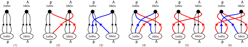
Figure 1: Diagrammatic representation of the four-point correlation function $\langle p\Lambda\overline{p\Lambda_{\mathrm{dsu}}}\rangle$. The interpolating field $\Lambda_{\mathrm{dsu}}$ is used as a representative of $\Lambda$.

2.1 Classification with respect to quark lines on the source side

Since this algorithm does not impose any restrictions on the quark fields on each baryon in the source, there is no need for each quark field in the source to be spatially identical between the baryons. The Wick contraction can be performed appropriately no matter what quantum state is considered. This algorithm fully preserves the internal degrees of freedom of each three-quark field contained in the two baryons on the source side. Therefore, allowing us to classify in detail which baryon on the source side the quark propagation in each baryon block comes from.

In the Fig. 1, each baryon block contains three quark lines connected from the source side. We classify which of the two baryons on the source side those quark lines come from; there are $2^{3}=8$ possibilities in general for a baryon block. If all three quark lines come from the first (second) baryon, i.e., $\overline{p}_{\alpha_{3}}$ ($\overline{\Lambda}_{\alpha_{4}}$), it is labeled as [111] ([222]). When the three quark lines come from different baryons, they are indicated by one of the remained six combinations as [211], [121], [221], [112], [212], or [122], so as to correctly represent the quark lines connect from the which of the two baryons on the source side.

$p^{(1)},\Lambda^{(1)}$	$p^{(2)},\Lambda^{(2)}$	$p^{(3)},\Lambda^{(3)}$	$p^{(4)},\Lambda^{(4)}$	$p^{(5)},\Lambda^{(5)}$	$p^{(6)},\Lambda^{(6)}$
[111],[222]	[112],[221]	[121],[122]	[122],[121]	[112],[221]	[122],[121]

Table 1: Classification which of two baryons on the source side the quark lines come from in each baryon block for the $\langle p\Lambda\overline{p\Lambda_{\mathrm{dsu}}}\rangle$ correlation function according to Eqs. (3) $-$ (21). The first (second) square brackets show the first (second) baryon block, i.e., proton ($\Lambda$).

Table 1 shows the classification of baryon blocks to calculate the $\langle p\Lambda\overline{p\Lambda_{\mathrm{dsu}}}\rangle$ correlation function according to Eqs. (3) $-$ (21). If we calculate only one particular single channel correlation function such a classification might not be very useful. However, in order to execute efficiently a large number of high performance computing jobs with huge electric power, it is beneficial to perform a simultaneous HPC job for various $BB$ channels. Here, for example, we will calculate the correlation functions of 52 channels, from $NN$ to $\Xi\Xi$:

$$\!\!\!\!\!\!\!\!\!\!\!\!\langle pn\overline{pn}\rangle,~{}$$ (28)

$$\!\!\!\!\!\!\!\!\!\!\!\!\!\!\!\!\begin{array}[]{lll}\langle p\Lambda\overline{p\Lambda}\rangle,&\langle p\Lambda\overline{\Sigma^{+}n}\rangle,&\langle p\Lambda\overline{\Sigma^{0}p}\rangle,\\ \langle\Sigma^{+}n\overline{p\Lambda}\rangle,&\langle\Sigma^{+}n\overline{\Sigma^{+}n}\rangle,&\langle\Sigma^{+}n\overline{\Sigma^{0}p}\rangle,\\ \langle\Sigma^{0}p\overline{p\Lambda}\rangle,&\langle\Sigma^{0}p\overline{\Sigma^{+}n}\rangle,&\langle\Sigma^{0}p\overline{\Sigma^{0}p}\rangle,\end{array}$$ (32)

$$\!\!\!\!\!\!\!\!\!\!\!\!\!\!\!\!\begin{array}[]{llllll}\langle\Lambda\Lambda\overline{\Lambda\Lambda}\rangle,&\!\!\!\!\langle\Lambda\Lambda\overline{p\Xi^{-}}\rangle,&\!\!\!\!\langle\Lambda\Lambda\overline{n\Xi^{0}}\rangle,&\!\!\!\!\langle\Lambda\Lambda\overline{\Sigma^{+}\Sigma^{-}}\rangle,&\!\!\!\!\langle\Lambda\Lambda\overline{\Sigma^{0}\Sigma^{0}}\rangle,\\ \langle p\Xi^{-}\overline{\Lambda\Lambda}\rangle,&\!\!\!\!\langle p\Xi^{-}\overline{p\Xi^{-}}\rangle,&\!\!\!\!\langle p\Xi^{-}\overline{n\Xi^{0}}\rangle,&\!\!\!\!\langle p\Xi^{-}\overline{\Sigma^{+}\Sigma^{-}}\rangle,&\!\!\!\!\langle p\Xi^{-}\overline{\Sigma^{0}\Sigma^{0}}\rangle,&\!\!\!\!\langle p\Xi^{-}\overline{\Sigma^{0}\Lambda}\rangle,{}\\ \langle n\Xi^{0}\overline{\Lambda\Lambda}\rangle,&\!\!\!\!\langle n\Xi^{0}\overline{p\Xi^{-}}\rangle,&\!\!\!\!\langle n\Xi^{0}\overline{n\Xi^{0}}\rangle,&\!\!\!\!\langle n\Xi^{0}\overline{\Sigma^{+}\Sigma^{-}}\rangle,&\!\!\!\!\langle n\Xi^{0}\overline{\Sigma^{0}\Sigma^{0}}\rangle,&\!\!\!\!\langle n\Xi^{0}\overline{\Sigma^{0}\Lambda}\rangle,{}\\ \langle\Sigma^{+}\Sigma^{-}\overline{\Lambda\Lambda}\rangle,&\!\!\!\!\langle\Sigma^{+}\Sigma^{-}\overline{p\Xi^{-}}\rangle,&\!\!\!\!\langle\Sigma^{+}\Sigma^{-}\overline{n\Xi^{0}}\rangle,&\!\!\!\!\langle\Sigma^{+}\Sigma^{-}\overline{\Sigma^{+}\Sigma^{-}}\rangle,&\!\!\!\!\langle\Sigma^{+}\Sigma^{-}\overline{\Sigma^{0}\Sigma^{0}}\rangle,&\!\!\!\!\langle\Sigma^{+}\Sigma^{-}\overline{\Sigma^{0}\Lambda}\rangle,{}\\ \langle\Sigma^{0}\Sigma^{0}\overline{\Lambda\Lambda}\rangle,&\!\!\!\!\langle\Sigma^{0}\Sigma^{0}\overline{p\Xi^{-}}\rangle,&\!\!\!\!\langle\Sigma^{0}\Sigma^{0}\overline{n\Xi^{0}}\rangle,&\!\!\!\!\langle\Sigma^{0}\Sigma^{0}\overline{\Sigma^{+}\Sigma^{-}}\rangle,&\!\!\!\!\langle\Sigma^{0}\Sigma^{0}\overline{\Sigma^{0}\Sigma^{0}}\rangle,{}\\ &\!\!\!\!\langle\Sigma^{0}\Lambda\overline{p\Xi^{-}}\rangle,&\!\!\!\!\langle\Sigma^{0}\Lambda\overline{n\Xi^{0}}\rangle,&\!\!\!\!\langle\Sigma^{0}\Lambda\overline{\Sigma^{+}\Sigma^{-}}\rangle,&&\!\!\!\!\langle\Sigma^{0}\Lambda\overline{\Sigma^{0}\Lambda}\rangle,\end{array}$$ (39)

$$\!\!\!\!\!\!\!\!\!\!\!\!\!\!\!\!\begin{array}[]{lll}\langle\Xi^{-}\Lambda\overline{\Xi^{-}\Lambda}\rangle,&\langle\Xi^{-}\Lambda\overline{\Sigma^{-}\Xi^{0}}\rangle,&\langle\Xi^{-}\Lambda\overline{\Sigma^{0}\Xi^{-}}\rangle,{}\\ \langle\Sigma^{-}\Xi^{0}\overline{\Xi^{-}\Lambda}\rangle,&\langle\Sigma^{-}\Xi^{0}\overline{\Sigma^{-}\Xi^{0}}\rangle,&\langle\Sigma^{-}\Xi^{0}\overline{\Sigma^{0}\Xi^{-}}\rangle,{}\\ \langle\Sigma^{0}\Xi^{-}\overline{\Xi^{-}\Lambda}\rangle,&\langle\Sigma^{0}\Xi^{-}\overline{\Sigma^{-}\Xi^{0}}\rangle,&\langle\Sigma^{0}\Xi^{-}\overline{\Sigma^{0}\Xi^{-}}\rangle,{}\end{array}$$ (43)

$$\!\!\!\!\!\!\!\!\!\!\!\!\langle\Xi^{-}\Xi^{0}\overline{\Xi^{-}\Xi^{0}}\rangle.~{}$$ (44)

In the circumstance, we need to know exactly in which channel each baryon block is required, and which baryon on the source side each quark line is associated with as a result of the Wick’s contraction.

Baryon block		[111]	[211]	[121]	[221]	[112]	[212]	[122]	[222]	Total
Proton	$X_{\mathrm{udu}}$	18	0	31	0	106	16	121	12	304
$\Sigma^{+}$	$X_{\mathrm{usu}}$	3	0	10	0	52	3	55	1	124
$\Xi^{0}$	$X_{\mathrm{uss}}$	16	19	0	0	118	102	29	14	298
$\Lambda_{\mathrm{dsu}}$	$X_{\mathrm{dsu}}$	242	318	436	408	290	266	376	248	2584
$\Lambda_{\mathrm{sud}}$	$X_{\mathrm{sud}}$	94	164	102	132	130	164	102	96	984
$\Lambda_{\mathrm{uds}}$	$X_{\mathrm{uds}}$	94	102	130	102	164	132	164	96	984

Table 2: Numbers how many times each baryon block is declared in the whole calculation of 52 correlation functions given in Eqs. (28)$-$(44). The baryon block is classified into eight $(=2^{3})$ forms with respect to which of two baryons on the source side the quark lines come from.

Table 2 summarizes the classification of the numbers of baryon blocks needed to calculate all 52 4pt-correlators of the $BB$ channels with respect to the forms that their quark lines connect. In the 2+1 flavor calculation, since isospin symmetry holds, the propagators of the up and down quarks are numerically the same, and the classification with respect to neutron can be included in the proton. Similarly, the classification for $\Sigma^{-}$ ($\Xi^{-}$) is contained in the $\Sigma^{+}$ ($\Xi^{0}$). The classification concerning $\Sigma^{0}$ can be included in $\Lambda$. If we use the interpolating field of $\Sigma^{0}$ as $\Sigma^{0}={1\over{\sqrt{2}}}\left(X_{\mathrm{dsu}}+X_{\mathrm{usd}}\right)$, both of the classifications for $\Sigma^{0}_{\mathrm{dsu}}$ and $\Sigma^{0}_{\mathrm{usd}}$ are included in $\Lambda_{\mathrm{dsu}}$. The numbers of $\Lambda_{\mathrm{dsu}}$ block declared in the whole calculation become larger than the numbers of other baryon blocks declared in the Table 2.

3 Numerical results

In this section, we present the results of the system with strangeness $S=-1$ at nearly physical quark masses corresponding to $(m_{\pi},m_{K})=(146,525)$ MeV with large volume $(La)^{4}=(96a)^{4}=(8.1~{}\mathrm{fm})^{4}$. Earlier results had already been reported at LATTICE 2017 [6]; the lattice setup is basically the same as that in Ref. [6]. We increase the number of statistics to the double from the number in the Ref. [6]. For a more detail of the lattice setup, please refer to the earlier report [6].

3.1 $\Lambda N$ potential

In order to obtain the single-channel $\Lambda N$ potential, we first extract the $R$-correlator projected on to appropriate angular momentum $(J,M)$ state from the 4pt-correlator

$$\begin{array}[]{c}{R}_{\alpha_{1}\alpha_{2}}^{\langle p\Lambda\overline{p\Lambda}\rangle}(\vec{r},t-t_{0};JM)={\rm e}^{(m_{p}+m_{\Lambda})(t-t_{0})}\sum_{\alpha_{3}\alpha_{4}}P_{\alpha_{3}\alpha_{4}}^{(J,M)}{F}_{\alpha_{1}\alpha_{2},\alpha_{3}\alpha_{4}}^{\langle p\Lambda\overline{p\Lambda}\rangle}(\vec{r},t-t_{0}).\end{array}$$ (45)

For the spin triplet state, the $R$ is further decomposed into the $S$- and $D$-wave components as

$$\left\{\begin{array}[]{l}R(\vec{r};\ ^{3}S_{1})={\cal P}R(\vec{r};J=1)\equiv{1\over 24}\sum_{{\cal R}\in{O}}{\cal R}R(\vec{r};J=1),\\ R(\vec{r};\ ^{3}D_{1})={\cal Q}R(\vec{r};J=1)\equiv(1-{\cal P})R(\vec{r};J=1).\end{array}\right.$$ (46)

Two central and tensor potentials, $V^{\mathrm{(Central)}}(r;J=0)=(V^{(0)}(r)-3V^{(\sigma)}(r))$ for $J=0$, $V^{\mathrm{(Central)}}(r;J=1)=(V^{(0)}(r)+V^{(\sigma)}(r))$, and $V^{\mathrm{(Tensor)}}(r)$ for $J=1$, are determined from the Schrödinger equation.

$$\left\{\begin{array}[]{c}V^{\mathrm{(C)}}(r;J=0){R}(\vec{r},t-t_{0};J=0)=\left({\nabla^{2}\over 2\mu}-{\partial\over\partial t}\right){R}(\vec{r},t-t_{0};J=0),\\ \left\{\begin{array}[]{c}{\cal P}\\ {\cal Q}\end{array}\right\}\times\left\{V^{\mathrm{(C)}}(r;J=1)+V^{(T)}(r)S_{12}\right\}{R}(\vec{r},t-t_{0};J=1)\par=\left\{\begin{array}[]{c}{\cal P}\\ {\cal Q}\end{array}\right\}\times\left\{{\nabla^{2}\over 2\mu}-{\partial\over\partial t}\right\}{R}(\vec{r},t-t_{0};J=1).\end{array}\right.$$ (47)

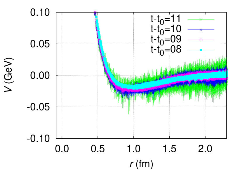
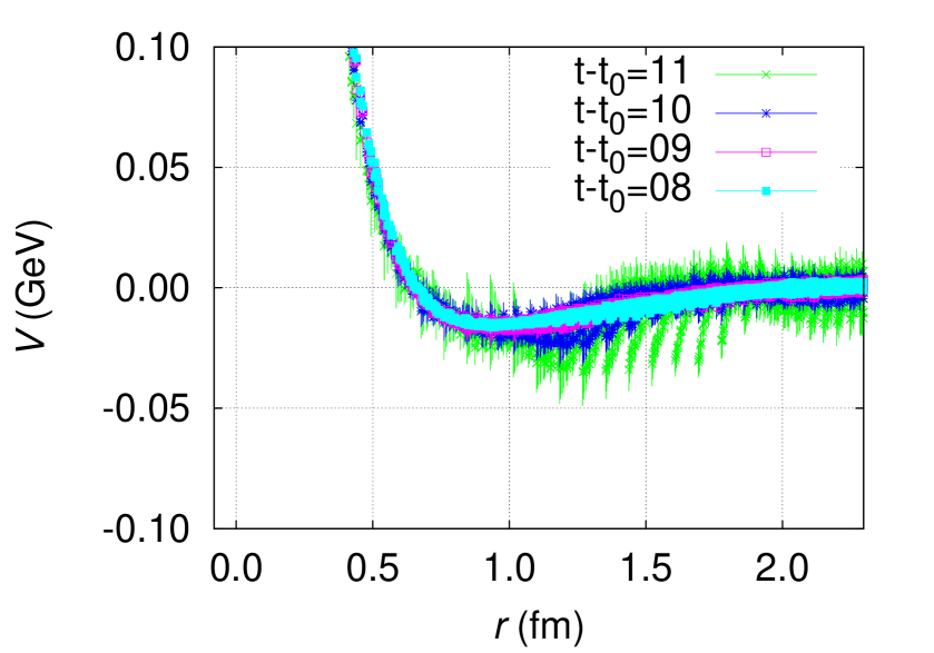
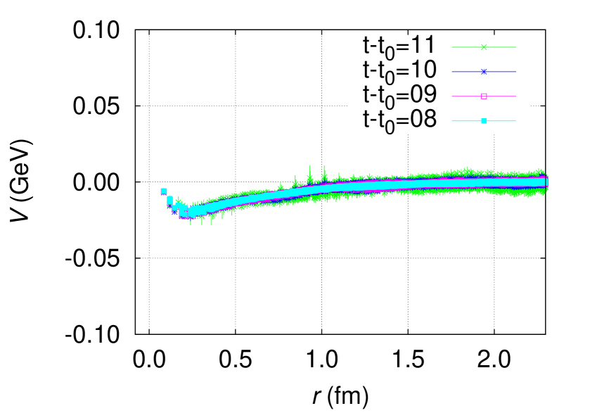
Figure 2: Three $\Lambda N$ single-channel potentials of (i) ${}^{1}S_{0}$ central (left), (ii) ${}^{3}S_{1}-^{3}D_{1}$ central (center), and (iii) ${}^{3}S_{1}-^{3}D_{1}$ tensor (right).

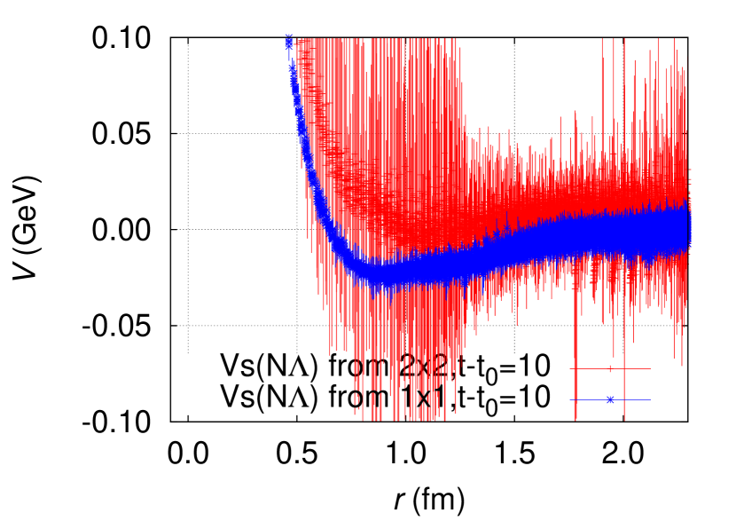
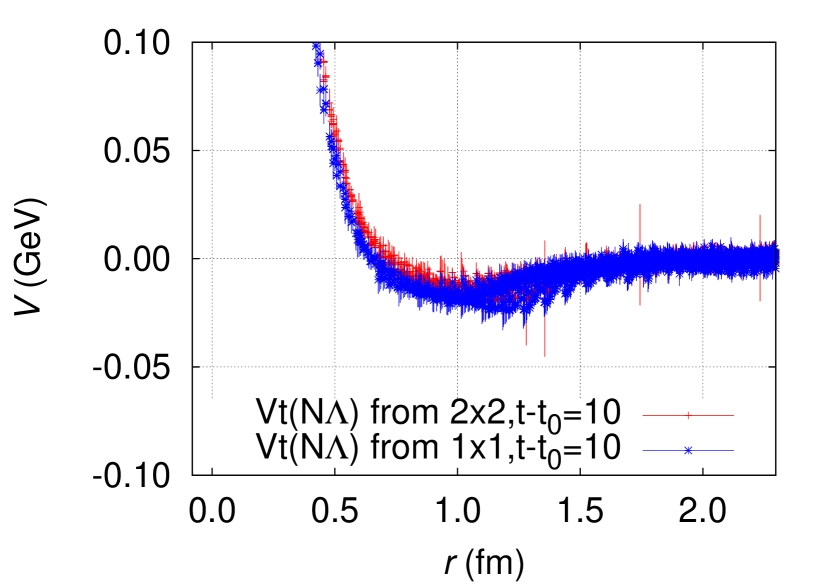
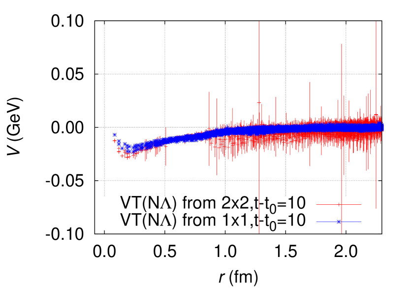
Figure 3: Comparisons between the $\Lambda N-\Lambda N$ diagonal part in $2\times 2$ coupled-channel potential and the $\Lambda N$ single channel potential, for (i) ${}^{1}S_{0}$ central (left), (ii) ${}^{3}S_{1}-^{3}D_{1}$ central (center), and (iii) ${}^{3}S_{1}-^{3}D_{1}$ tensor (right).

Fig. 2 shows three potentials of the $\Lambda N$ system; (i) the central potential in the ${}^{1}S_{0}$ (left), (ii) the central potential in the ${}^{3}S_{1}-^{3}D_{1}$ (center), and (iii) the tensor potential in the ${}^{3}S_{1}-^{3}D_{1}$ (right). These potentials are obtained through the single channel formulation of the HAL QCD method, which are valid below the $\Sigma N$ threshold and the effects by coupling with the $\Sigma N$ channel are implicitly included. Both the ${}^{1}S_{0}$ and ${}^{3}S_{1}-^{3}D_{1}$ central potentials have short ranged repulsive core and medium-to-long-distanced attractive well. These two potentials are more or less similar to each other. For flavor $SU(3)$ symmetric case, the $\Lambda N$ state is represented in terms of irreducible representation (irrep.) in flavor space as $|\Lambda N,^{1}S_{0}\rangle={1\over{\sqrt{10}}}\left(3|{\bm{27}}\rangle+|{\bm{8}}_{\mathrm{s}}\rangle\rangle\right)$, and $|\Lambda N,^{3}E_{1}\rangle={1\over{\sqrt{2}}}\left(|\overline{\bm{10}}\rangle-|{\bm{8}}_{\mathrm{a}}\rangle\right)$, while the $NN$ state is given by $|NN,~{}^{1}S_{0}\rangle=|{\bm{27}}\rangle$, and $|NN,~{}^{3}E_{1}\rangle=|\overline{\bm{10}}\rangle$. These single channel $\Lambda N$ ${}^{1}S_{0}$ and ${}^{3}S_{1}-^{3}D_{1}$ potentials are qualitatively similar to the $NN$ ${}^{1}S_{0}$ and ${}^{3}S_{1}-^{3}D_{1}$ potentials, respectively, though the flavor structures of the $\Lambda N$ are not the same as those of the $NN$. Observing the central potentials in detail, the ${}^{1}S_{0}$ potential gradually changes to become a little attractive when the time slice increases from $t=8$ to $9$ but the change is unclear at $t=10,11$ due to the large statistical uncertainty; this behavior reflects to the scattering phase shifts shown in the next subsection. On the other hand, such a deviation of the potential in the ${}^{3}S_{1}-^{3}D_{1}$ channel is little; the central values of the potential hardly change over time to time but the statistical uncertainty increases.

Fig. 3 shows the comparisons between the $\Lambda N$ potential from the single channel analysis and the $\Lambda N-\Lambda N$ diagonal part from the coupled-channel analysis using $\Lambda N$ and $\Sigma N$ correlation functions. The statistical uncertainty of the $\Lambda N-\Lambda N$ diagonal part of the coupled-channel potential in the ${}^{1}S_{0}$ is large and it dramatically reduces by taking the single channel $\Lambda N$ potential. For the ${}^{3}S_{1}-^{3}D_{1}$ state, the single channel $\Lambda N$ central potential slightly enhances the attraction from the $\Lambda N-\Lambda N$ diagonal part of the coupled-channel potential. The short distance part of the single channel $\Lambda N$ tensor potential is slightly suppressed from the $\Lambda N-\Lambda N$ diagonal part of the coupled-channel potential.

3.2 Scattering phase shifts

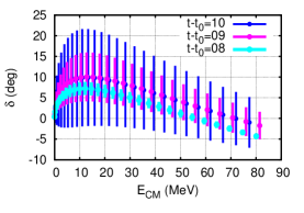
Figure 4: Scattering phase shift in the ${}^{1}S_{0}$ state of $\Lambda N$ system, obtained by solving the Schrödinger equation with parametrized functional form in Ref. [6].

By employing the single channel analysis for the $\Lambda N$ low-energy state the statistical errors are significantly reduced. Thus we parametrize the potentials with the analytic functional form in Ref. [6]. Figure 4 shows the scattering phase shift in ${}^{1}S_{0}$ channel obtained through the parametrized $\Lambda N$ potential. The present result shows that the interaction in the ${}^{1}S_{0}$ channel is attractive on average in the low-energy region though the fluctuation is large.

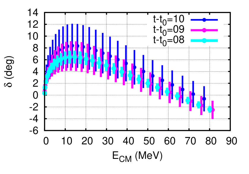
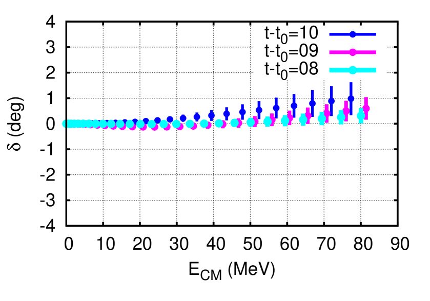
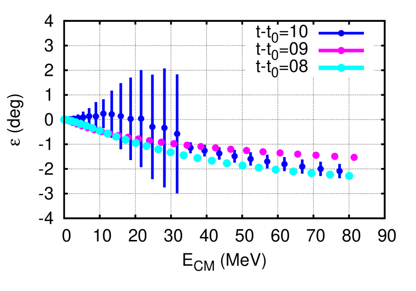
Figure 5: Scattering bar-phase shifts and mixing angle in the ${}^{3}S_{1}-^{3}D_{1}$ states of $\Lambda N$ system, $\bar{\delta}_{0}$ (left), $\bar{\delta}_{2}$ (center), and $\bar{\varepsilon}_{1}$ (right), obtained by solving the Schrödinger equation with parametrized functional form in Ref. [6].

Figure 5 shows the scattering phase shifts in ${}^{3}S_{1}-^{3}D_{1}$ channels. For the ${}^{3}S_{1}-^{3}D_{1}$ channels, the scattering matrix is parametrized with three real parameters bar-phase shifts and mixing angle. The phase shift $\bar{\delta}_{0}$ at the time slices $t-t_{0}=8-10$ shows the interaction is attractive. Because of large statistical uncertainty, it is hard to see how large is the spin-spin interaction $(V^{(\sigma)})$ of the $\Lambda N$ interaction.

Both the strengths of attraction in $\delta(^{1}S_{0})$ and $\bar{\delta}_{0}$ seem to be weaker than the usual empirical values such as Ref. [9]; it might be due to a little deviation of light quark mass which is corresponding to $(m_{\pi},m_{K})\approx(146,525)$ MeV. For both Figs. 4 and 5, the parametrizing procedure is not very stable, especially for $V^{(\sigma)}$ and $V^{(T)}$. The present phase shifts and mixing angle are preliminary results at this moment.

4 Discussion

We present the phase shifts of low energy $\Lambda N$ scattering by using the potential extracted from lattice QCD through the HAL QCD method. Both the spin singlet and triplet states are weakly attractive in low energy region, which are qualitatively in good agreement with empirical studies. However, the strengths of the attraction seem to be weaker than the phenomenological conclusion. In addition, statistical uncertainty is still large to pin down the spin-spin interaction of the $\Lambda N$ system. Since the present results still have a large uncertainty, we need to continue our calculations based on the following points. (i) employ the physical quark masses which is more precisely close to the real system (but practically we should apply the 2+1 flavor approach for a while), (ii) using a sufficiently large volume, (iii) to endeavor for clarifying various details to reduce the statistical and/or systematic uncertainty.

In this report, the numerical results are obtained by using the wall quark sources, where the quark field is uniform and identical in all spatial directions even between the baryons. The effective block algorithm presented in this report can be applied for more flexible choices of interpolating field on the source side; this should be a strong advantageous to improve the present large uncertainty. We hope an improved calculation will be reported in the future.

References

- [1] P. Demorest, T. Pennucci, S. Ransom, M. Roberts and J. Hessels, Shapiro Delay Measurement of A Two Solar Mass Neutron Star, Nature 467 (2010) 1081 [1010.5788].
- [2] J. Antoniadis et al., A Massive Pulsar in a Compact Relativistic Binary, Science 340 (2013) 6131 [1304.6875].
- [3] E. Fonseca et al., Refined Mass and Geometric Measurements of the High-mass PSR J0740+6620, Astrophys. J. Lett. 915 (2021) L12 [2104.00880].
- [4] HAL QCD collaboration, Lattice QCD approach to Nuclear Physics, PTEP 2012 (2012) 01A105 [1206.5088].
- [5] HAL QCD collaboration, An implementation of hybrid parallel C++ code for the four-point correlation function of various baryon-baryon systems, PoS LATTICE2013 (2014) 426.
- [6] H. Nemura et al., Baryon interactions from lattice QCD with physical masses — strangeness sector —, EPJ Web Conf. 175 (2018) 05030 [1711.07003].
- [7] H. Nemura, Instructive discussion of an effective block algorithm for baryon–baryon correlators, Comput. Phys. Commun. 207 (2016) 91 [1510.00903].
- [8] H. Nemura et al., A Fast Algorithm for Lattice Hyperonic Potentials, JPS Conf. Proc. 17 (2017) 052002 [1604.08346].
- [9] J. Haidenbauer, U.G. Meißner and A. Nogga, Hyperon–nucleon interaction within chiral effective field theory revisited, Eur. Phys. J. A 56 (2020) 91 [1906.11681].