Joint Time-Vertex Fractional Fourier Transform

Abstract

Graphs signal processing successfully captures high-dimensional data on non-Euclidean domains by using graph signals defined on graph vertices. However, data sources on each vertex can also continually provide time-series signals such that graph signals on each vertex are now time-series signals. Joint time-vertex Fourier transform (JFT) and the associated framework of time-vertex signal processing enable us to study such signals defined on joint time-vertex domains by providing spectral analysis. Just as the fractional Fourier transform (FRT) generalizes the ordinary Fourier transform (FT), we propose the joint time-vertex fractional Fourier transform (JFRT) as a generalization to the JFT. JFRT provides an additional fractional analysis tool for joint time-vertex processing by extending both temporal and vertex domain Fourier analysis to fractional orders. We theoretically show that the proposed JFRT generalizes the JFT and satisfies the properties of index additivity, reversibility, reduction to identity, and unitarity (for certain graph topologies). We provide theoretical derivations for JFRT-based denoising as well as computational cost analysis. Results of numerical experiments are also presented to demonstrate the benefits of JFRT.

Index Terms - Graph signal processing (GSP), fractional Fourier transform, time-vertex processing, graph Fourier transform (GFT), signal processing on graphs, graphs, joint time-vertex Fourier transform (JFT).

I Introduction

With the increasing amount of complex data residing on irregular domains with complex interactions, the need for novel analysis and processing tools to deal with them has emerged. A prevalent approach of representing and processing data with inherently irregular and/or complex structures is the actively developing field of graph signal processing (GSP) [1, 2, 3, 4, 5, 6, 7, 8, 9, 10, 11, 12, 13, 14]. Within the framework of GSP, two standard signal processing approaches have been adopted [2, 10]. The first approach is based on the concept of Laplacian matrix [2, 12, 1] while the second one, stemming from algebraic signal processing, is based on graph adjacency matrices, which are also referred as graph shift operators [1, 3, 4, 5, 6, 7, 8, 9, 10, 11, 13].

In recent years, a wide range of signal processing methods has been generalized to the GSP domain. Those include sampling and approximation [6, 15, 16, 17], filtering [1, 2, 3, 18, 19],[7, 9, 10, 11, 13, 20], interpolation [16], Fourier transformation and its duality [1, 21, 22, 23, 24], and frequency analysis [5, 13, 25]. The generalization of the Fourier transform (FT) for graph signals, which is called the graph Fourier transform (GFT), along with other GSP techniques, gave rise to numerous applications including smoothing and denoising [26, 27, 28, 29, 19], segmentation [30], classification [31], [32], clustering [33, 34], low-rank extraction [35], stationary signals and spectral estimation [36, 37], non-stationary analysis [38, 39], semi-supervised learning [40, 31], multiscale decompositions [41, 39, 38, 42, 43], stationary process processing [36, 37], signal prediction [44], graph learning [45, 46, 47], intrusion detection [48], machine learning [49], and deep learning [22, 50, 51, 52].

While vertices and edges are of primary interest in GSP to model non-Euclidean graph data, the time domain information in vertices can also be important. Moreover, time domain information is generally a natural extension. For example, while the distribution of weather stations in a region forms a graph, these stations are also recording daily and in some cases hourly measurements. Similarly sensor networks are naturally interconnected and have also their own history of measurements. In other words, data defined on the vertices of graphs change over time and the applications like above make the analysis of joint time-vertex signals important. This spurs a need for a framework in which the temporal graph data can be processed jointly with the vertex domain. The tools developed by the pioneering works of [53, 54, 25, 55] combine the temporal discrete signal processing and GSP. Referred as the time-vertex signal processing, these important techniques enable us to work with time-varying graph signals by considering both temporal and graph-domain information. As the main joint Fourier analysis tool to obtain spectral expansions of joint time-vertex signals, the joint time-vertex Fourier transform (JFT) has been developed [25, 53]. JFT combines FT in the temporal domain and GFT in the vertex domain[25, 53]. Time domain information in time-vertex signals may be deterministic [25] or stationary processes [55]. Autoregressive moving average (ARMA) and vector autoregressive moving average (VARMA) filters for processing of time-vertex graph signals are developed [56, 57]. Time-vertex signal processing is deployed in several applications including reconstruction of time-varying graph signals [58, 59, 60], predicting the joint spectral temporal data [57], and predicting the evolution of stationary graph signals [61]. There are also applications of semi-supervised learning and inpainting of joint-time vertex signals [55, 61, 54]. Spatio-temporal graph applications can also be seen as joint time-vertex signals, and there are transform and filtering considerations for such applications [62, 63].

The $\alpha$th order fractional Fourier transform (FRT) is defined as the $\alpha$th power of the ordinary Fourier transform (FT). FRT reduces to the FT and the identity operations when $\alpha$ = 1 and $\alpha$ = 0, respectively [64, 65, 66, 67, 68, 69, 70, 71]. The ordinary FT is a transformation between time (or space) signals into spectral signals, whereas FRT makes conversions into intermediate domains between time (or space) and frequency (spatial frequency). Thus, it can be viewed as a linear transformation corresponding to a rotation in the time-frequency plane. FRT has the property of additive indexes, meaning that the $\alpha$th order of $\beta$th order FRT is equal to the $(\alpha+\beta)$th order FRT.

FRT is a fundamental transform that has important applications in several fields including signal processing, optics, and wave propagation [67]. The applications of FRT in signal processing include time-frequency analysis [72, 69], filter design [73, 74, 75, 76], image processing [77, 78, 79], video processing [79], beamforming [80, 81], pattern recognition [82], phase retrieval [83], optical information processing [64], [82], sonar signal processing [84], inverse synthetic-aperture radar (ISAR) imaging [85] among numerous others. FRT provides extra degrees of freedom when transforming signals into intermediate time-frequency domains while keeping the ordinary FT as a special case. This feature of FRT gives flexibility in processing data and makes performance improvements possible, mostly without additional computational costs. Similarly, extending FRT to the GSP domain can open up further developments, application areas, and performance increases. To this end, graph FRTs (GFRTs), which transform graph signals into intermediate vertex-frequency or vertex-spectral domains, have been introduced very recently [8, 11, 86, 87, 88, 89]. Furthermore, windowed fractional Fourier transform has been generalized to GSP [86, 87] and sampling in fractional domains is studied [11]. Very recently, the Wiener filtering has also been studied in the GSP domain [90], where the optimal filtering happens in intermediate domains.

To extend the recent theoretical studies of joint time-vertex signal processing, we introduce the joint time-vertex fractional Fourier Transform (JFRT), which analyses signals in both graph fractional and time fractional domains simultaneously. We show that JFRT has the properties of index additivity in both domains, reduction to the ordinary transformation when the orders are 1 in both domains, reduction to the identity operator when the orders are 0, commutativity and reversibility. We also show that if ordinary GFT is unitary, then so is the JFRT and show that JFRT reduces to the two dimensional discrete FRT (DFRT) for certain graph topologies. To develop the theory further, we also present the underlying theoretical setting for Tikhonov regularization-based denoising by the proposed JFRT. To this end, we present some properties of fractional Laplacians and define the joint fractional Laplacian to derive the optimal filter coefficients in the JFRT domain.

The proposed JFRT, with the flexibility provided by its two fractional order parameters, can be utilized in joint time-vertex signal processing applications such as denoising, signal reconstruction, graph-node classification since it enables the joint signal to be processed both in FRT and GFRT domains. This makes it possible to analyze joint time-vertex signals in a much wider class of transformations by extending the theory of ordinary JFT analysis. Since JFRT satisfies most of the underlying properties of the two dimensional DFRT, it is also a good candidate for the generalization of multidimensional FRTs to GSP. On the other side of the coin, the proposed JFRT also contributes to the well-established and rich literature on the fractional Fourier analysis by extending the classical theory to the realm of GSP machinery.

The rest of the manuscript is organized as follows. In Section II, we provide preliminary information for GSP, GFT, JFT and FRT. We introduce the definition of the proposed JFRT in Section III and provide its properties. In Section IV, we present the Tikhonov regularization-based denoising in the JFRT domain. Section V shows the utility of JFRT through numerical experiments and examples in denoising and clustering tasks. Section VI concludes the paper.

Notation

Bold capital letters denote matrices while small capital letters denote vectors. Given a set $\mathcal{V}$, $|\mathcal{V}|$ denotes its cardinality. $()^{*}$, $()^{T}$, $()^{H}$ denotes complex conjugate, transpose and complex conjugate transpose (Hermitian) of their argument. If the argument of $diag(.)$ is an ordered set, it constructs a square matrix with elements of the ordered set as diagonal elements. If the argument is matrix, it gives a column vector containing the diagonal entries of the matrix. $\mathbf{I}_{n}$ denotes an identity matrix of size $n$ and we omit the subscript if the context is clear. For given matrices $\mathbf{A}$ and $\mathbf{B}$, $\mathbf{A}\otimes\mathbf{B}$ denote their Kronecker product, and if $\mathbf{A}\in\mathbb{C}^{m\times m}$, $\mathbf{B}\in\mathbb{C}^{n\times n}$ are square matrices, $\mathbf{A}\oplus\mathbf{B}=\mathbf{A}\otimes\mathbf{I}_{n}+\mathbf{I}_{m}\otimes\mathbf{B}$ denotes their Kronecker sum. For scalars $N$, $M$, the modulo $M$ of $N$ is denoted by $(N)_{M}$.

II Preliminaries

In this section, preliminaries on graph signals, GFTs, graph fractional Fourier transforms (GFRT), continuous and discrete fractional Fourier transforms and joint time-vertex Fourier transform (JFT) are provided.

II-A Graph Signals

Let $\mathcal{G}=\{\mathcal{V},\mathcal{E},\mathbf{A}\}$ be a graph with $|\mathcal{V}|=N\in\mathbb{Z}^{+}$ where $\mathcal{V}=\{v_{0},v_{1},...,v_{N-1}\}$ is the set of nodes (vertices), $\mathcal{E}$ is the set of edges and $\mathbf{A}\in\mathbb{C}^{N\times N}$ is the adjacency matrix of $\mathcal{G}$. An edge $e=(m,n)$ is an element of $\mathcal{E}$ if $\mathbf{A}_{m,n}\neq 0$ where $\mathbf{A}_{m,n}$ denotes the element in the intersection of $m$th row and $n$th column, otherwise there is no connection from node $m$ to node $n$. A graph is undirected if $\mathbf{A}_{m,n}=\mathbf{A}_{n,m}$ for all $m,n\in\{0,1,...,N-1\}$. A graph signal $\mathbf{x}\in\mathbb{C}^{N}$ is a mapping from $\mathcal{V}$ to $\mathbb{C}^{N}$ [1, 3] such that:

$$\mathbf{x}:\mathcal{V}\rightarrow\mathbb{C}^{N}$$

$$v_{n}\rightarrow\mathbf{x}_{n}.$$

II-B Graph Fourier Transform (GFT)

There are several approaches to define GFT [2, 1, 91, 92, 93]. Among them, two main approaches stand out. The first one follows the algebraic signal processing framework that views the adjacency matrices as a shift operator and builds a GFT definition accordingly [1]. The second one uses the graph Laplacian, which is defined for undirected graphs with non-negative weighted adjacency matrices [2].

II-B1 Algebraic Signal Processing Based Approach

Let $\mathbf{A}=\mathbf{V}\mathbf{J}_{\mathbf{A}}\mathbf{V}^{-1}$ be the Jordan decomposition of $\mathbf{A}$. Then, GFT is defined as

$$\mathbf{F}_{G}\mathbf{x}=\mathbf{V}^{-1}\mathbf{x}=\mathbf{\tilde{x}},$$ (1)

where $\mathbf{\tilde{x}}$ stands for the graph signal in GFT domain with GFT matrix $\mathbf{F}_{G}:=\mathbf{V}^{-1}$. We have the inverse transform as

$$\mathbf{F}_{G}^{-1}\mathbf{\tilde{x}}=\mathbf{V}\mathbf{\tilde{x}}=\mathbf{x}.$$ (2)

This approach has the advantage that it can be used for any type of graph while having the disadvantage that it uses the Jordan decomposition, which is computationally costly compared to the graph Laplacian based approach for large graphs.

II-B2 Graph (Combinatorial) Laplacian Based Approach

In the graph Laplacian based approach, the adjacency matrix $\mathbf{A}$ takes non-negative real values and it is assumed to be symmetric. The graph Laplacian can be given as $\mathbf{L}=\mathbf{D}-\mathbf{A}$ where $\mathbf{D}_{m,m}=\sum_{n=0}^{N-1}\mathbf{A}_{m,n}$ is the diagonal degree matrix. Then, we have $\mathbf{L}=\mathbf{U}\Lambda\mathbf{U}^{H}$ as the diagonalization of $\mathbf{L}$. Since $\mathbf{L}$ is symmetric positive semi-definite, it is unitarily diagonalizable. Then, the GFT can be defined as the following [2]:

$$\mathbf{F}_{G}\mathbf{x}=\mathbf{U}^{H}\mathbf{x}=\mathbf{\tilde{x}},$$ (3)

where $\mathbf{\tilde{x}}$ is the representation of graph signal $\mathbf{x}$ in the graph Fourier (spectral) domain with $\mathbf{F}_{G}:=\mathbf{U}^{H}$. One can obtain the inverse transformation as:

$$\mathbf{F}^{-1}\mathbf{\tilde{x}}=\mathbf{U}\mathbf{\tilde{x}}=\mathbf{x}.$$ (4)

Although there are attempts for generalizations [93], the Laplacian-based approach is generally considered to be limited to undirected graphs. However, the Laplacian-based GFT has the advantage of providing a unitary transformation so that the Parseval’s relation holds.

In this work, we consider an arbitrary GFT matrix as denoted by $\mathbf{F}_{G}$, which can be built by using either of the two approaches or any other approach that represents the GFT as an invertible matrix.

II-C Fractional Fourier Transform (FRT)

The $\alpha$th order FRT $\mathcal{F}^{\alpha}$ can be defined as follows for $\alpha\in\mathbb{R}$:

$$\mathcal{F}^{\alpha}f(u)=\int_{-\infty}^{\infty}K_{\alpha}(u,u)f(u^{\prime})du^{\prime},$$ (5)

$$K_{\alpha}(u,u)=A_{\theta}e^{(j\pi(u^{2}cot\theta-2uu^{\prime}csc\theta+u^{\prime 2}cot\theta))},$$ (6)

$$A_{\theta}=\frac{e^{-j\pi\text{sgn}(\text{sin}\theta)/4+j\theta/2}}{\left|\text{sin}\theta\right|^{1/2}}\text{ and }\theta=\frac{\alpha\pi}{2},$$ (7)

where $0<\left|\alpha\right|<2$. More details of FRT can be found in [67].

II-D Discrete Fractional Fourier Transform (DFRT)

The DFRT is defined as the following [94]:

$$\mathbf{F}^{\alpha}[m,n]=\sum_{k=0,k\neq N-1(N)_{2}}^{N}\mathbf{u}_{k}[m]e^{-j\frac{\pi}{2}k\alpha}\mathbf{u}_{k}[n],$$ (8)

where $\mathbf{u}_{k}$ is the discrete counterpart of the $k$th Hermite-Gaussian function and $(N)_{2}$ is the modulo 2 of $N$. The peculiar range of summation occurs because of the number of zero crossings of the discrete Hermite Gaussian functions, which are the eigenvectors of the normalized discrete Fourier transform (DFT) matrix. The DFRT is unitary, index additive, and reduces to the identity and DFT when $\alpha=0$ and $\alpha=1$, respectively. Further details can be found in [94].

II-E Graph Fractional Fourier Transform (GFRT)

Let the GFT matrix be $\mathbf{F}_{G}=\mathbf{P}\mathbf{J}_{G}\mathbf{P}^{-1}$ be the Jordan decomposition of $\mathbf{F}_{G}$. Then, GFRT can be defined as [8]:

$$\mathbf{F}_{G}^{\alpha}=\mathbf{P}\mathbf{J}_{G}^{\alpha}\mathbf{P}^{-1},$$ (9)

where $\alpha\in\mathbb{R}$ is the fractional order. For computing $\mathbf{J}_{G}^{\alpha}$, for the $m$th Jordan block with the eigenvalue $\lambda_{m}$, $\alpha$th power of the $k$th super-diagonal can be given as $\prod_{n=1}^{k}\frac{\alpha+1-n}{n}\lambda_{m}^{\alpha-k}$. The additional details of computing (9) can be found in [8]. This definition of GFRT is index additive as:

$$\mathbf{F}_{G}^{\alpha}\mathbf{F}_{G}^{\beta}=\mathbf{P}\mathbf{J}_{G}^{\alpha}\mathbf{P}^{-1}\mathbf{P}\mathbf{J}_{G}^{\beta}\mathbf{P}^{-1}=\mathbf{P}\mathbf{J}_{G}^{\alpha}\mathbf{J}_{G}^{\beta}\mathbf{P}^{-1}$$

$$=\mathbf{P}\mathbf{J}_{G}^{\alpha+\beta}\mathbf{P}^{-1}=\mathbf{F}_{G}^{\alpha+\beta}.$$ (10)

GFRT has also the properties of reduction to the identity matrix and to the GFT matrix when orders are $\alpha=0$ and $\alpha=1$, respectively.

II-F Joint time-vertex Fourier Transform (JFT)

Let $\mathbf{X}\in\mathbb{C}^{N\times T}$ represent the joint time-vertex signal such that we have graph signals in the columns and time-series signals defined for each vertex of the underlying graph in the rows of $\mathbf{X}$. The DFT of this signal is given as:

$$\text{DFT}(\mathbf{X})=\mathbf{X}\mathbf{F}^{T},$$ (11)

where $\mathbf{F}$ is the normalized DFT matrix with its elements given as $(\mathbf{F})_{m,n}=\exp(\frac{-j2\pi mn}{T}),\text{ }m,n=0,1,...,T-1$. Similarly, the GFT of $\mathbf{X}$ can be given as:

$$\text{GFT}(\mathbf{X};\mathcal{G})=\mathbf{F}_{G}\mathbf{X}.$$ (12)

Finally, the JFT of $\mathbf{X}$ is defined as [53, 25]

$$\text{JFT}(\mathbf{X};\mathcal{G})=\mathbf{F}_{G}\mathbf{X}\mathbf{F}^{T},$$ (13)

which is able to capture the spectral information of $\mathbf{X}$ in both time and underlying graph perspectives. To define the transform in a more compact form, one can denote JFT in matrix form by vectorizing $\mathbf{X}$. Doing so, we have:

$$\text{JFT}(\mathbf{x},\mathcal{G})=\mathbf{F}_{J}\mathbf{x}$$ (14)

where $\mathbf{F}_{J}:=\mathbf{F}\otimes\mathbf{F}_{G}$ and $\mathbf{x}=vec(\mathbf{X})$. The inverse JFT is given by:

$$\text{JFT}^{-1}(\mathbf{X},G)=\mathbf{F}_{G}^{-1}\mathbf{X}\mathbf{F}^{*},$$ (15)

and $\mathbf{F}_{J}^{-1}=\mathbf{F}^{H}\otimes\mathbf{F}_{G}^{-1}$. It is shown in [53] that if the underlying $\mathbf{F}_{G}$ is unitary, so is JFT.

II-G The Graph Fractional Laplacian

Let $\mathbf{L}=\mathbf{U}\mathbf{\Lambda}\mathbf{U}^{H}$ be the diagonalization of a graph Laplacian. Then the graph fractional Laplacian of the order $\alpha$ can be defined as [87]:

$$\mathbf{L}_{\alpha}=\mathbf{U}^{\alpha}\mathbf{\Lambda}^{\alpha}(\mathbf{U}^{\alpha})^{H}.$$ (16)

III The Joint Time-Vertex Fractional Fourier Transform (JFRT)

In this section, we define JFRT as a joint generalization of JFT to fractional Fourier and fractional graph Fourier domains. Let $\mathbf{X}\in\mathbb{C}^{N\times T}$ holds a joint time-vertex signal defined on the graph $\mathcal{G}$, where $N$ is the number of vertices of $\mathcal{G}$ and $T$ is the length of the time-series signals defined on each vertex. Then, we define for the order pair $(\alpha,\beta)$ where $\alpha$, $\beta\in\mathbb{R}$, the $(\alpha,\beta)$th order JFRT as the following:

$$\text{JFT}^{\alpha,\beta}(\mathbf{X};\mathcal{G}):=\mathbf{F}_{G}^{\beta}\mathbf{X}(\mathbf{F}^{\alpha})^{T},$$ (17)

where $\mathbf{F}_{G}^{\beta}$ is the $\beta$th order GFRT defined by (9) and $\mathbf{F}^{\alpha}$ is the $\alpha$th order FRT as defined in (8). Note that $\mathbf{F}_{G}$ can be constructed from an arbitrary approach. Note that (17), is a linear transformation from $N\times T$ sized matrices to $N\times T$ sized matrices, that is $\text{JFT}^{\alpha,\beta}(.):\mathbb{C}^{N\times T}\rightarrow\mathbb{C}^{N\times T}$. If we vectorize the given time-vertex signal $\mathbf{X}$ as $\mathbf{x}=vec(\mathbf{X})$, we can find an equivalent transformation between the vectorized forms as $\mathbf{F}_{J}^{\alpha,\beta}(.):\mathbb{C}^{NT}\rightarrow\mathbb{C}^{NT}$. From the properties of the Kronecker product, such a mapping can be explicitly stated as $\mathbf{F}_{J}^{\alpha,\beta}:=\mathbf{F}^{\alpha}\otimes\mathbf{F}_{G}^{\beta}$ in the matrix form.

III-A Essential properties of JFRT

In what follows, we present important propositions and properties of the proposed JFRT operation.

Property 1.

For two real-valued pairs $(\alpha_{1},\beta_{1})$ and $(\alpha_{2},\beta_{2})$,

$$\text{{JFT}}^{\alpha_{1},\beta_{1}}(\text{{JFT}}^{\alpha_{2},\beta_{2}}(\mathbf{X};\mathcal{G});\mathcal{G})=\text{{JFT}}^{\alpha_{1}+\alpha_{2},\beta_{1}+\beta_{2}}(\mathbf{X},\mathcal{G}).$$ (18)

In other words, JFRT is index additive in fractional orders.

Proof.

By definition, we have:

$$\text{JFT}^{\alpha_{1},\beta_{1}}(\text{JFT}^{\alpha_{2},\beta_{2}}(\mathbf{X};\mathcal{G});\mathcal{G})=\mathbf{F}_{G}^{\beta_{1}}\mathbf{F}_{G}^{\beta_{2}}\mathbf{X}(\mathbf{F}^{\alpha_{2}})^{T}(\mathbf{F}^{\alpha_{1}})^{T}$$

$$=\mathbf{F}_{G}^{\beta_{1}}\mathbf{F}_{G}^{\beta_{2}}\mathbf{X}(\mathbf{F}^{\alpha_{1}}\mathbf{F}^{\alpha_{2}})^{T}=\mathbf{F}_{G}^{\beta_{1}+\beta_{2}}\mathbf{X}(\mathbf{F}^{\alpha_{1}+\alpha_{2}})^{T},$$

where the last equality follows from the index additivity properties of GFRT and FRT. ∎

Property 2.

For two real-valued pairs $(\alpha_{1},\beta_{1})$ and $(\alpha_{2},\beta_{2})$, JFRT is commutative such that

$$\text{{JFT}}^{\alpha_{1},\beta_{1}}(\text{{JFT}}^{\alpha_{2},\beta_{2}}(\mathbf{X};\mathcal{G});\mathcal{G})=\text{{JFT}}^{\alpha_{2},\beta_{2}}(\text{{JFT}}^{\alpha_{1},\beta_{1}}(\mathbf{X};\mathcal{G});\mathcal{G}).$$ (19)

JFRT is also cross commutative such that:

$$\text{{JFT}}^{\alpha_{1},\beta_{1}}(\text{{JFT}}^{\alpha_{2},\beta_{2}}(\mathbf{X};\mathcal{G});\mathcal{G})=\text{{JFT}}^{\alpha_{1},\beta_{2}}(\text{{JFT}}^{\alpha_{2},\beta_{1}}(\mathbf{X};\mathcal{G});\mathcal{G})$$

$$=\text{{JFT}}^{\alpha_{2},\beta_{1}}(\text{{JFT}}^{\alpha_{1},\beta_{2}}(\mathbf{X};\mathcal{G});\mathcal{G}).$$ (20)

Proof.

This property follows from the index additivity property:

$$\text{JFT}^{\alpha_{1},\beta_{1}}(\text{JFT}^{\alpha_{2},\beta_{2}}(\mathbf{X};\mathcal{G});\mathcal{G})=(\text{JFT}^{\alpha_{1}+\alpha_{2},\beta_{1}+\beta_{2}}(\mathbf{X};\mathcal{G})$$

$$=\text{JFT}^{\alpha_{2},\beta_{2}}(\text{JFT}^{\alpha_{1},\beta_{1}}(\mathbf{X};\mathcal{G});\mathcal{G})$$ (21)

The cross commutativity also follows from the index additivity:

$$\text{JFT}^{\alpha_{1},\beta_{1}}(\text{JFT}^{\alpha_{2},\beta_{2}}(\mathbf{X};\mathcal{G});\mathcal{G})=\text{JFT}^{\alpha_{1}+\alpha_{2},\beta_{1}+\beta_{2}}(\mathbf{X};\mathcal{G})$$

$$=\text{JFT}^{\alpha_{1},\beta_{2}}(\text{JFT}^{\alpha_{2},\beta_{1}}(\mathbf{X};\mathcal{G});\mathcal{G})$$

$$=\text{JFT}^{\alpha_{2},\beta_{1}}(\text{JFT}^{\alpha_{1},\beta_{2}}(\mathbf{X};\mathcal{G});\mathcal{G}),$$ (22)

where the last equality follows from commutativity. ∎

Property 3.

$\text{{JFT}}^{0,0}(\mathbf{X};\mathcal{G})=\mathbf{X}$, which is the reduction to the identity property.

Proof.

This simply follows from the definition of JFRT and the reduction to the identity properties of FRT and GFRT. ∎

Property 4.

JFRT is separable over graph fractional transform and DFRT, that is for a given order $(\alpha,\beta)$ we have:

$$\text{{JFT}}^{\alpha,\beta}(\mathbf{X};\mathcal{G})=\text{{JFT}}^{0,\beta}(\text{{JFT}}^{\alpha,0}(\mathbf{X};\mathcal{G}))=\text{{JFT}}^{0,\beta}(\text{{JFT}}^{\alpha,0}(\mathbf{X};\mathcal{G}))$$ (23)

Proof.

First equality follows from the index additivity property while the second follows from the commutativity property. Notice that from the reduction to the identity properties of GFRT and DFRT, and using the definition of JFRT, we have the equation (23) as:

$$\mathbf{F}_{G}^{\beta}\mathbf{X}\mathbf{F}^{\alpha}=\mathbf{F}_{G}^{\beta}(\mathbf{I}_{N}\mathbf{X}\mathbf{F}^{\alpha})\mathbf{I}_{T}=\mathbf{I}_{N}(\mathbf{F}_{G}^{\beta}\mathbf{X}\mathbf{I}_{T})\mathbf{F}^{\alpha}$$ (24)

which clearly shows the separable nature of JFRT. ∎

Property 5.

For an order pair $(\alpha,\beta)$, JFRT is reversible, i.e. we have $\text{{JFT}}^{-\alpha,-\beta}(\text{{JFT}}^{\alpha,\beta}(\mathbf{X};\mathcal{G});\mathcal{G})=\mathbf{X}$.

Proof.

This simply follows from the index additivity and the reduction to the identity properties of JFRT. ∎

Property 6.

Reduction to the ordinary transformation property as given by $\text{{JFT}}^{1,1}(\mathbf{X};\mathcal{G})=\text{{JFT}}(\mathbf{X};\mathcal{G})$.

Proof.

This also follows from the definition of JFRT and the reduction to the ordinary transform properties of FRT and GFRT. Thus, JFT becomes a special case of JFRT when order $(1,1)$. ∎

Proposition 1.

If $\mathbf{F}_{G}$ is a unitary transformation, then so is $\text{{JFT}}^{\alpha,\beta}(\mathbf{X;\mathcal{G}})$ or equivalently $\mathbf{F}_{J}^{\alpha,\beta}$ is a unitary matrix.

Proof.

From the properties of the Kronecker product, we know that if $\mathbf{F}^{\alpha}$ and $\mathbf{F}_{G}^{\beta}$ are unitary matrices, then so is $\mathbf{F}_{J}^{\alpha,\beta}$. We know that $\mathbf{F}^{\alpha}$ is unitary for any $\alpha$ by the properties of FRT [67]. Hence, we only need to show that if $\mathbf{F}_{G}$ is unitary, then $\mathbf{F}_{G}^{\beta}$ is also unitary for any $\beta$. If $\mathbf{F}_{G}$ is unitary, it can be diagonalized as $\mathbf{F}_{G}=\mathbf{V}_{G}\mathbf{\Lambda}_{G}\mathbf{V}_{G}^{H}$ with unitary $\mathbf{V}_{G}$ and diagonal $\mathbf{\Lambda}_{G}$ with eigenvalues lying on the unit circle. Then, $\mathbf{F}_{G}^{\beta}=\mathbf{V}_{G}\mathbf{\Lambda}_{G}^{\beta}\mathbf{V}_{G}^{H}$ will also be unitary since the diagonal values of $\mathbf{\Lambda}_{G}^{\beta}$ will be on the unit circle as well. ∎

Hence, for unitary $\mathbf{F}_{G}$, JFRT is also a unitary transform satisfying the Parseval’s relation.

It is known that for directed circular graphs, DFT diagonalizes the adjacency matrix, and that for an undirected ring graph, DFT diagonalizes the Laplacian matrix. Therefore, for these particular graphs, the GFT can be taken as the DFT matrix or we can perceive time-series data as a graph in the shape of a directed circular graph or undirected ring graph [1]. Then, we have the following proposition:

Proposition 2.

If the underlying graph is directed circular graph or ring graph, then $\text{{JFT}}^{\alpha,\beta}(\mathbf{X;\mathcal{G}})$ reduces to two dimensional DFRT with orders $\alpha$ and $\beta$.

Proof.

We have $\text{JFT}^{\alpha,\beta}(\mathbf{X};\mathcal{G})=\mathbf{F}_{G}^{\beta}\mathbf{X}(\mathbf{F}^{\alpha})^{T}$. Then, one can reduce $\mathbf{F}_{G}$ to $\mathbf{F}$ due to the underlying graph as follows: From (8), it can be seen that for even $N$,

$$\mathbf{F}_{G}=\mathbf{V}_{F}diag\{e^{-j\frac{\pi}{2}0},e^{-j\frac{\pi}{2}1},...,e^{-j\frac{\pi}{2}(N-1)}\}\mathbf{V}_{F}^{H}$$

is a unitary diagonalization of $\mathbf{F}$ where $\mathbf{V}_{F}=[\mathbf{u}_{0},\mathbf{u}_{1},...,\mathbf{u}_{N-1}]$ and $\mathbf{u}_{k}$’s are the discrete Hermite-Gaussians. Then, we have

$$\mathbf{F}_{G}^{\beta}=\mathbf{V}_{F}diag\{e^{-j\frac{\pi}{2}0\beta},...,e^{-j\frac{\pi}{2}(N-1)\beta}\}\mathbf{V}_{F}^{H}=\mathbf{F}^{\beta}.$$ (25)

A similar diagonalization can also be made for odd $N$. Hence, we obtain $\text{JFT}^{\alpha,\beta}(\mathbf{X};\mathcal{G})=\mathbf{F}^{\beta}\mathbf{X}(\mathbf{F}^{\alpha})^{T}$ which is equivalent to the two dimensional DFRT of $\mathbf{X}$. ∎

Corrolary 1.

If the underlying graphs are either directed circular graph or ring graph, then $\text{{JFT}}^{1,1}(\mathbf{X},\mathcal{G})$ can be represented as two dimensional DFT.

Proof.

This follows from the previous proposition and reduction to the ordinary transform property of FRT. ∎

As a two dimensional transformation, JFRT has the properties of index additivity, reduction to the identity and reduction to the ordinary transformations just as the two dimensional DFRT. It also has the property of unitarity provided that $\mathbf{F}_{G}$ is unitary. This condition is satisfied for undirected graphs with common GFT definitions [1, 2]. Also, there are unitary transformations for the directed graphs introduced by recent works [95]. Therefore, JFRT is a good candidate that generalizes the discrete manifestation of the two dimensional FRT (2D-DFRT) of the classical signal processing to the GSP domain.

III-B Computational Cost Analysis

Since both JFT and JFRT are separable, their computational complexity analysis can be done separately for time domain and graph domain transformations. In JFT, we take the DFT of $N$ rows in $\mathcal{O}(NT\log T)$ complexity using the fast Fourier transform (FFT). Similarly, for a $T$ length vector, its DFRT can also be efficiently computed by using the established fast algorithm in [96]. Hence taking DFRT of $N$ rows has the complexity of $\mathcal{O}(NT\log T)$ as well. For graph transformations, the computational cost of taking a GFT of a vector of length $N$ is $\mathcal{O}(N^{2})$ since it is a matrix-vector multiplication. Although there are works that reduce the computational cost in obtaining exact or approximate transforms [97, 98, 99, 100] for certain classes of graphs, there are no generalized fast GFT computation algorithms like the FFT and the fast DFRT. Since GFRT is also in a matrix form, transforming $T$ columns is of complexity $\mathcal{O}(TN^{2})$ for both GFT and GFRT. This gives a total complexity of $\mathcal{O}(NT(\log T+N))$ for calculating either JFT or JFRT. Thus, in terms of transformation complexity, JFRT brings no extra computational burden.

In the case of JFRT filtering, consider a filter $h(\lambda,\omega)$ with $\lambda=\lambda_{1},...\lambda_{N}$, $\omega=\omega_{1},...,\omega_{T}$, let $\mathbf{X}\in\mathbb{C}^{N\times T}$ be a joint time-vertex signal and let the graph Laplacian of the underlying graph be $\mathbf{L}$. For the ordinary JFT, the FFT of every row is first computed with the computational complexity $\mathcal{O}(NT\log T)$. Then for each column of $\mathbf{X}$, a $k$th order Chebyshev approximation of $h(\lambda,\omega_{k})$, where $\omega_{k}=2\pi k/T$, $k=0,1,...,T-1$, is computed with the computational complexity $\mathcal{O}(KT|\mathcal{E}|)$, where $\mathcal{E}$ is the set of edges for the underlying graph [25]. Then, the inverse FFT of each row is calculated with complexity $\mathcal{O}(NT\log T)$. For JFRT filtering, one again looks at $\mathcal{O}(NT\log T)$ complexity for taking DFRTs of every row since DFRTs can also be efficiently computed in $\mathcal{O}(T\log T)$ time [96]. Then, we filter each column of $\mathbf{X}$ with $h_{frac}(\lambda,\omega)$. Since we have already computed the diagonalization of $\mathbf{L}$ to obtain GFRT, we can filter each column of $\mathbf{X}$ using the already obtained GFRT. Hence, effectively, we reach the total computational complexity of $\mathcal{O}(N^{2}T)$ for the computation of GFRT filtering of each column. Lastly, the inverse DFRT of each column is calculated with $\mathcal{O}(NT\log T)$ complexity.

IV Tikhonov regularization-based denoising with JFRT

In this section, we present the underlying theoretical setting for Tikhonov regularization-based denoising by the proposed JFRT. In doing so, we first present some properties of fractional Laplacians and define joint fractional Laplacian, then we introduce a fractional variation measure, and show the connection of Tikhonov regularization with joint fractional Laplacians. These are then used to derive regularization-based denoising by JFRT and to find the optimal filter in fractional time-vertex domains.

IV-A Graph, Time and Joint Fractional Laplacians

Let us first remember the definitions of edge derivative and graph gradient. In the graph Laplacian approach, for a graph signal $\mathbf{x}\in\mathbb{R}^{N}$, the edge derivative with respect to the edge $e=(m,n)$ at vertex $m$ can be given as [53, 2]:

$$\left.\frac{\partial\mathbf{x}}{\partial e}\right|_{m}=\sqrt{\mathbf{A}_{m,n}}[\mathbf{x}_{m}-\mathbf{x}_{n}],$$ (26)

where $\mathbf{A}$ is the adjacency matrix of the given graph. Then the graph gradient of $\mathbf{x}$ at vertex $m$ can also be given as [53, 2]:

$$\left.\nabla_{G}\mathbf{x}_{m}\right|_{m}=\Big{\{}\left.\frac{\partial\mathbf{x}}{\partial e}\right|_{m}\Big{\}}_{e\in\mathcal{E}}.$$ (27)

Without the loss of generality, once an ordering of edges are set, the graph gradient can be represented as a matrix $\bm{\nabla}_{G}\in\mathbb{R}^{|\mathcal{E}|\times N}$ with elements:

$$(\bm{\nabla}_{G})_{k,m}=\begin{cases}\sqrt{\mathbf{A}_{m,n}},\text{ if }e_{k}=(m,n),\\ -\sqrt{\mathbf{A}_{m,n}},\text{ if }e_{k}=(n,m),\\ 0,\text{ otherwise},\end{cases}$$ (28)

where $e_{k}$ is the $k$th edge where $k=1,2,...,|\mathcal{E}|$. Then the graph divergence of the graph gradient gives the graph Laplacian as $\mathbf{L}_{G}=(\bm{\nabla}_{G})^{T}(\bm{\nabla}_{G})$. Similarly, a $T$-dimensional time-series signal can be thought of a circular ring graph [2, 1]. For circular ring graphs, we have:

$$\mathbf{(A_{circ})}_{m,n}=\begin{cases}1\text{ if }|(m-n)_{T}|=1,\\ 0,\text{otherwise}.\end{cases}$$ (29)

Let $e_{1}=(1,2)$, $e_{2}=(2,3)$, … , $e_{T-1}=(T-1,T)$, $e_{T}=(T,1)$, then let the graph gradient of circular ring graph be $\bm{\nabla}_{T}$. Notice that $\bm{\nabla}_{T}$ is the first order difference operator such that $(\bm{\nabla}_{T}\mathbf{x})_{m}=\mathbf{x}_{m}-\mathbf{x}_{(m-1)_{N}}$. We then finally have the time Laplacian as $\mathbf{L}_{T}=(\bm{\nabla}_{T})^{T}\bm{\nabla}_{T}$ [2, 25].

For a fractional order $\alpha$, as we have given in Section II-G, we have the graph fractional Laplacian as $(\mathbf{L_{G}})_{\alpha}=\mathbf{U}_{G}^{\alpha}\mathbf{\Lambda}^{\alpha}(\mathbf{U}_{G}^{\alpha})^{H}$. It is known that the graph Laplacian is a positive semi-definite Hermitian matrix [2]. Next, we show that the graph fractional Laplacian is also positive semi-definite Hermitian matrix:

Proposition 3.

For any fractional order $\alpha$, $(\mathbf{L_{G}})_{\alpha}$ is a positive semi-definite Hermitian matrix.

Proof.

We have $(\mathbf{L_{G}})_{\alpha}=\mathbf{U}_{G}^{\alpha}\mathbf{\Lambda}^{\alpha}(\mathbf{U}_{G}^{\alpha})^{H}$. Define $\mathbf{M}_{G}=\mathbf{\Lambda}^{\alpha/2}(\mathbf{U}_{G}^{\alpha})^{H}$. Notice that since $(\mathbf{L_{G}})_{1}=\mathbf{L}_{G}$ is Hermitian, all of the elements of $\mathbf{\Lambda}$ are real. Then $(\mathbf{L_{G}})_{\alpha}=\mathbf{M}_{G}^{H}\mathbf{M}_{G}$ is Hermitian (by construction) and positive semi-definite since for any $\mathbf{x}\in\mathbb{C}^{N}$ we have

$$\mathbf{x}^{H}(\mathbf{L_{G}})_{\alpha}\mathbf{x}=\mathbf{x}^{H}\mathbf{M}_{G}^{H}\mathbf{M}_{G}\mathbf{x}=(\mathbf{M}_{G}\mathbf{x})^{H}\mathbf{M}_{G}\mathbf{x}\geq 0.$$

∎

Now, recall that the diagonalizations of the time and graph fractional Laplacians are given as $(\mathbf{L}_{T})_{\alpha}=\mathbf{U}_{T}^{\alpha}\mathbf{\Lambda}_{T}^{\alpha}(\mathbf{U}_{T}^{\alpha})^{H}$ and $(\mathbf{L}_{G})_{\beta}=\mathbf{U}_{G}^{\beta}\mathbf{\Lambda}_{G}^{\beta}(\mathbf{U}_{G}^{\beta})^{H}$ for fractional orders $\alpha$ and $\beta$, respectively. We can now define the joint fractional Laplacian $\mathbf{L}_{J}^{(\alpha,\beta)}$ as the Krocnecker sum of the time and graph fractional Laplacians as parallel to the construction of the ordinary joint Laplacian [25] :

$$\mathbf{L}_{J}^{(\alpha,\beta)}:=(\mathbf{L}_{T})_{\alpha}\oplus(\mathbf{L}_{G})_{\beta}=(\mathbf{L}_{T})_{\alpha}\otimes\mathbf{I}_{G}+\mathbf{I}_{T}\otimes(\mathbf{L}_{G})_{\beta}$$

$$=(\mathbf{U}_{T}^{\alpha}\mathbf{\Lambda}_{T}^{\alpha}(\mathbf{U}_{T}^{\alpha})^{H})\otimes\mathbf{I}_{G}+\mathbf{I}_{T}\otimes(\mathbf{U}_{G}^{\beta}\mathbf{\Lambda}_{G}^{\beta}(\mathbf{U}_{G}^{\beta})^{H})$$

$$=(\mathbf{U}_{T}^{\alpha}\otimes\mathbf{U}_{G}^{\beta})(\mathbf{\Lambda}_{T}^{\alpha}\oplus\mathbf{\Lambda}_{G}^{\beta})(\mathbf{U}_{T}^{\alpha}\otimes\mathbf{U}_{G}^{\beta})^{H}$$

$$=\mathbf{U}_{J}^{(\alpha,\beta)}\mathbf{\Lambda}_{J}^{(\alpha,\beta)}(\mathbf{U}_{J}^{(\alpha,\beta)})^{H}.$$ (30)

By noticing that $(\mathbf{U}_{J}^{(\alpha,\beta)})^{H}=(\mathbf{U}_{T}^{\alpha}\otimes\mathbf{U}_{G}^{\beta})^{H}=\mathbf{F}^{\alpha}\otimes(\mathbf{F}_{G}^{\beta})=\mathbf{F}_{J}^{(\alpha,\beta)}$, the eigenvector matrices obtained from the diagonalization of the joint fractional Laplacian form a basis for the JFRT. Conversely, JFRT diagonalizes the joint fractional Laplacian.

Proposition 4.

For any fractional order pair $(\alpha,\beta)$, the joint fractional Laplacian is a positive semi-definite Hermitian matrix.

Proof.

For the Hermitian, by the definition given in (30), we need to only show that $\mathbf{\Lambda}_{J}^{(\alpha,\beta)}$ is Hermitian. From Proposition 3, $\mathbf{\Lambda}_{T}^{\alpha}$ and $\mathbf{\Lambda}_{G}^{\beta}$ are non-negative real-valued diagonal matrices. In (30), $\mathbf{\Lambda}_{J}^{(\alpha,\beta)}=(\mathbf{\Lambda}_{T}^{\alpha}\oplus\mathbf{\Lambda}_{G}^{\beta})$ is also real-valued diagonal matrix due to the properties of the Kronecker sum, hence it is Hermitian. From the diagonalization of $\mathbf{L}_{J}^{(\alpha,\beta)}$ in (30), Hermitian property follows.

For positive semi-definiteness, let $\mathbf{M}_{J}:=(\mathbf{\Lambda}_{J}^{(\alpha,\beta)})^{0.5}(\mathbf{U}_{J}^{(\alpha,\beta)})^{H}$. Then we have $\mathbf{L}_{J}^{(\alpha,\beta)}=\mathbf{M}_{J}^{H}\mathbf{M}_{J}$. Thus, for any $\mathbf{x}\in\mathbb{C}^{NT}$ we have

$$\mathbf{x}^{H}\mathbf{L}_{J}^{(\alpha,\beta)}\mathbf{x}=\mathbf{x}^{H}\mathbf{M}_{J}^{H}\mathbf{M}_{J}\mathbf{x}=(\mathbf{M}_{J}\mathbf{x})^{H}(\mathbf{M}_{J}\mathbf{x})\geq 0.$$ (31)

∎

Below, we also provide some properties of JFT that will be used in the following subsection. First, we have the following relation for JFT [25]:

$$\bm{\nabla}_{J}\mathbf{x}=vec\Big{(}\begin{bmatrix}\mathbf{X}(\bm{\nabla}_{T})^{T}\\ (\bm{\nabla}_{G})\mathbf{X}\end{bmatrix}\Big{)},$$ (32)

where $\bm{\nabla}_{J}$ is the joint gradient and can be given as [25]:

$$\bm{\nabla}_{J}=\begin{bmatrix}(\bm{\nabla}_{T})\otimes\mathbf{I}_{G}\\ \mathbf{I}_{T}\otimes(\bm{\nabla}_{G})\end{bmatrix}.$$ (33)

Second, using (30) with order $(1,1)$, it can be shown that $\bm{\nabla}_{J}^{T}\bm{\nabla}_{J}=((\bm{\nabla}_{T})^{T}(\bm{\nabla}_{T}))\otimes\mathbf{I}_{G}+\mathbf{I}_{T}\otimes(\bm{\nabla}_{G})^{T}(\bm{\nabla}_{G})=(\mathbf{L}_{T})\otimes\mathbf{I}_{G}+\mathbf{I}_{T}\otimes(\mathbf{L}_{G})=\mathbf{L}_{J}^{(1,1)}=\mathbf{L}_{J}$.

We also define the joint fractional variation as the following:

$$\mathbf{x}^{H}\mathbf{L}_{J}^{(\alpha,\beta)}\mathbf{x}=\mathbf{x}^{H}((\mathbf{L}_{T})_{\alpha}\oplus(\mathbf{L}_{G})_{\beta})\mathbf{x},$$ (34)

which measures the variation of the input joint time-vertex signal $\mathbf{x}$ with respect to the JFRT modes that $(\mathbf{L}_{T})_{\alpha}$ and $(\mathbf{L}_{G})_{\beta}$ constitutes. Notice that for order (1,1), this reduces to the Laplacian quadratic form with ordinary joint Laplacian $\mathbf{L}_{J}^{(1,1)}=\mathbf{L}_{J}$ [2]. Since $\mathbf{L}_{J}^{(\alpha,\beta)}$ is positive semi-definite from Proposition 4, (34) gives non-negative real values.

IV-B Tikhonov Regularization with Joint Fractional Variation Measure

We have the following received joint time-vertex signal model in the Tikhonov regularization based denoising:

$$\mathbf{Y}=\mathbf{X}+\mathbf{N},$$ (35)

where $\mathbf{y}=vec(\mathbf{Y})$ is the received signal, $\mathbf{x}=vec(\mathbf{X})$ is the input signal, and $\mathbf{n}=vec(\mathbf{N})$ is the i.i.d. Gaussian noise distributed across two domains. For JFT, one way to denoise the received signal $\mathbf{y}$ is to minimize the following $l_{2}$ regularized objective function [25, 2]:

$$\mathbf{\hat{x}}=\operatorname*{arg\,min}_{\mathbf{x}=vec(\mathbf{X})}\|\left.\mathbf{y}-\mathbf{x}\right.\|_{2}^{2}+\tau_{g}\|\left.(\bm{\nabla})_{G}\mathbf{X}\right.\|_{F}^{2}+\tau_{t}\|\left.\mathbf{X}(\bm{\nabla})_{T}\right.\|_{F}^{2},$$ (36)

where $\tau_{g}$ and $\tau_{t}$ are non-negative real regularization parameters. One can show that the regularization component of (36) can be written as a Laplacian quadratic form:

$$\tau_{g}\|\left.(\bm{\nabla})_{G}\mathbf{X}\right.\|_{F}^{2}+\tau_{t}\|\left.\mathbf{X}(\bm{\nabla})_{T}\right.\|_{F}^{2}$$

$$=\|\left.\sqrt{\tau_{g}}(\bm{\nabla})_{G}\mathbf{X}\right.\|_{F}^{2}+\|\left.\mathbf{X}\sqrt{\tau_{t}}(\bm{\nabla})_{T}\right.\|_{F}^{2}$$

$$=\|\left.\bm{\nabla}_{J}^{\tau_{g},\tau_{t}}\mathbf{x}\right.\|_{2}^{2}=\mathbf{x}^{H}(\bm{\nabla}_{J}^{\tau_{g},\tau_{t}})^{T}(\bm{\nabla}_{J}^{\tau_{g},\tau_{t}})\mathbf{x}=\mathbf{x}^{H}\mathbf{L}_{J}^{\tau_{g},\tau_{t}}\mathbf{x},$$ (37)

where $\bm{\nabla}_{J}^{\tau_{g},\tau_{t}}$ denotes the regularized joint gradient as follows:

$$\bm{\nabla}_{J}^{\tau_{g},\tau_{t}}:=\begin{bmatrix}(\sqrt{\tau_{t}}\bm{\nabla}_{T})\otimes\mathbf{I}_{G}\\ \mathbf{I}_{T}\otimes(\sqrt{\tau_{g}}\bm{\nabla}_{G})\end{bmatrix},$$ (38)

and the regularized joint Laplacian $\mathbf{L}_{J}^{\tau_{g},\tau_{t}}:=(\bm{\nabla}_{J}^{\tau_{g},\tau_{t}})^{T}(\bm{\nabla}_{J}^{\tau_{g},\tau_{t}})$.

Second, since

$$\mathbf{L}_{J}^{\tau_{g},\tau_{t}}=(\bm{\nabla}_{J}^{\tau_{g},\tau_{t}})^{T}(\bm{\nabla}_{J}^{\tau_{g},\tau_{t}})$$

$$=((\sqrt{\tau_{t}}\bm{\nabla}_{T})\otimes\mathbf{I}_{G})^{T}((\sqrt{\tau_{t}}\bm{\nabla}_{T})\otimes\mathbf{I}_{G})+$$

$$(\mathbf{I}_{T}\otimes(\sqrt{\tau_{g}}\bm{\nabla}_{G}))^{T}(\mathbf{I}_{T}\otimes(\sqrt{\tau_{g}}\bm{\nabla}_{G}))$$

$$=((\sqrt{\tau_{t}}\bm{\nabla}_{T})^{T}(\sqrt{\tau_{t}}\bm{\nabla}_{T}))\otimes\mathbf{I}_{G}+\mathbf{I}_{T}\otimes((\sqrt{\tau_{g}}\bm{\nabla}_{G})^{T}(\sqrt{\tau_{g}}\bm{\nabla}_{G}))$$

$$=(\tau_{t}\mathbf{L}_{T})\otimes\mathbf{I}_{G}+\mathbf{I}_{T}\otimes(\tau_{g}\mathbf{L}_{G})=\tau_{t}(\mathbf{L}_{T})\oplus\tau_{g}(\mathbf{L}_{G}),$$ (39)

the regularized joint Laplacian can be written as the Kronecker sum of $\tau_{t}$-scaled time Laplacian and $\tau_{g}$-scaled graph Laplacian. By applying the definition of the joint fractional Laplacian given in (30) to the result obtained in (39), we can define a regularized joint fractional Laplacian $(\mathbf{L}_{J}^{\tau_{g},\tau_{t}})^{(\alpha,\beta)}$ by replacing ordinary time and graph Laplacians with fractional ones:

$$(\mathbf{L}_{J}^{\tau_{g},\tau_{t}})^{(\alpha,\beta)}:=\tau_{t}(\mathbf{L}_{T})_{\alpha}\oplus\tau_{g}(\mathbf{L}_{G})_{\beta}.$$ (40)

Now, we are in a position to use the regularized joint fractional Laplacian $(\mathbf{L}_{J}^{\tau_{g},\tau_{t}})^{(\alpha,\beta)}$ in parallel to the result obtained in (37) to do Tikhonov regularization across both graph fractional and time fractional domains by plugging it in (34) as a regularization parameter. Thus, we can write the regularization-based denoising objective function for JFRT as:

$$\mathbf{\hat{x}}=\operatorname*{arg\,min}_{\mathbf{x}=vec(\mathbf{X})}\|\left.\mathbf{y}-\mathbf{x}\right.\|_{2}^{2}+\mathbf{x}^{H}(\mathbf{L}_{J}^{\tau_{g},\tau_{t}})^{(\alpha,\beta)}\mathbf{x}.$$ (41)

The minimum value of (41) can be found as a filter in JFRT domain which we show in the following proposition.

Proposition 5.

$\mathbf{\hat{x}}=\mathbf{F}_{J}^{(-\alpha,-\beta)}\mathbf{H}_{J}^{(\alpha,\beta)}\mathbf{F}_{J}^{(\alpha,\beta)}\mathbf{y}$ is the minimizer in (41) where $\mathbf{H}_{J}^{(\alpha,\beta)}$ is the optimal multiplicative filter with diagonal elements given by:

$$diag(\mathbf{H}_{J}^{(\alpha,\beta)})=vec(\mathbf{H}^{(\alpha,\beta)}).$$ (42)

$\mathbf{H}^{(\alpha,\beta)}$ is the matrix manifestation of

$$h^{(\alpha,\beta)}_{m,n}=\frac{1}{1+\tau_{g}\lambda_{m}^{\beta}+\tau_{t}\omega_{n}^{\alpha}},$$ (43)

where $\lambda_{m}$ and $\omega_{n}$ are the eigenvalues of graph and time Laplacians with $m=1,2,...,N$ and $n=1,2,...,T$, respectively.

Proof.

Let $\mathbf{x}=\mathbf{x}_{r}+j\mathbf{x}_{j}$ where $\mathbf{x}_{r}$ and $\mathbf{x}_{j}$ are real valued vectors, and $j$ is the imaginary unit. Then since (41) is a convex function of $\mathbf{x}$, we can take the derivatives with respect to $\mathbf{x}_{r}$ and $\mathbf{x}_{j}$ and set them to zero. Let $f(\mathbf{x})$ be the argument of (41), i.e. $f(\mathbf{x})=(\mathbf{y}-\mathbf{x})^{H}(\mathbf{y}-\mathbf{x})+\mathbf{x}^{H}(\mathbf{L}_{J}^{\tau_{g},\tau_{t}})^{(\alpha,\beta)}\mathbf{x}$. By knowing that $(\mathbf{L}_{J}^{\tau_{g},\tau_{t}})^{(\alpha,\beta)}$ is an Hermitian matrix by Proposition 4, setting $\frac{\partial f(\mathbf{x})}{\partial\mathbf{x}_{r}}=0$ gives:

$$\Re\{\mathbf{y}\}=\mathbf{x}_{r}+\Re\{(\mathbf{L}_{J}^{\tau_{g},\tau_{t}})^{(\alpha,\beta)}\}\mathbf{x}_{r}-\Im\{(\mathbf{L}_{J}^{\tau_{g},\tau_{t}})^{(\alpha,\beta)}\}\mathbf{x}_{j},$$ (44)

where $\Re\{.\}$ and $\Im\{.\}$ are the real and imaginary parts of the complex argument, respectively. Similarly, setting $\frac{\partial f(\mathbf{x})}{\partial\mathbf{x}_{j}}=0$ yields:

$$\Im\{\mathbf{y}\}=\mathbf{x}_{j}+\Im\{(\mathbf{L}_{J}^{\tau_{g},\tau_{t}})^{(\alpha,\beta)}\}\mathbf{x}_{r}+\Re\{(\mathbf{L}_{J}^{\tau_{g},\tau_{t}})^{(\alpha,\beta)}\}\mathbf{x}_{j}.$$ (45)

Now we multiply (45) by $j$ and add to (44) to get:

$$\mathbf{y}=\mathbf{x}+(\mathbf{L}_{J}^{\tau_{g},\tau_{t}})^{(\alpha,\beta)}\mathbf{x}_{r}+j(\mathbf{L}_{J}^{\tau_{g},\tau_{t}})^{(\alpha,\beta)}\mathbf{x}_{j}=\mathbf{x}+(\mathbf{L}_{J}^{\tau_{g},\tau_{t}})^{(\alpha,\beta)}\mathbf{x}.$$ (46)

Using the mixed product property of the Kronecker product along with the diagonalization of $(\mathbf{L}_{G})_{\beta}$ and $(\mathbf{L}_{T})_{\alpha}$, we can now write:

$$(\mathbf{L}_{J}^{\tau_{g},\tau_{t}})^{(\alpha,\beta)}=(\tau_{t}\mathbf{L}_{T})_{\alpha}\otimes\mathbf{I}_{G}+\mathbf{I}_{T}\otimes(\tau_{g}\mathbf{L}_{G})_{\beta}$$

$$=(\mathbf{U}_{T}^{\alpha}(\tau_{t}\mathbf{\Lambda}_{T}^{\alpha})(\mathbf{U}_{T}^{\alpha})^{H})\otimes\mathbf{I}_{G}+\mathbf{I}_{T}\otimes(\mathbf{U}_{G}^{\beta}(\tau_{g}\mathbf{\Lambda}_{G}^{\beta})(\mathbf{U}_{G}^{\beta})^{H})$$

$$=(\mathbf{U}_{T}^{\alpha}\otimes\mathbf{U}_{G}^{\beta})(\tau_{t}\mathbf{\Lambda}_{T}^{\alpha}\oplus\tau_{g}\mathbf{\Lambda}_{G}^{\beta})(\mathbf{U}_{T}^{\alpha}\otimes\mathbf{U}_{G}^{\beta})^{H}$$

$$=\mathbf{U}_{J}^{(\alpha,\beta)}(\mathbf{\Lambda}_{J}^{\tau_{g},\tau_{t}})^{(\alpha,\beta)}(\mathbf{U}_{J}^{(\alpha,\beta)})^{H},$$ (47)

where $(\mathbf{\Lambda}_{J}^{\tau_{g},\tau_{t}})^{(\alpha,\beta)}:=(\tau_{t}\mathbf{\Lambda}_{T}^{\alpha}\oplus\tau_{g}\mathbf{\Lambda}_{G}^{\beta})$. Hence, JFRT also diagonalizes the regularized joint fractional Laplacian.

Then, using (47), we have the optimal $\mathbf{\hat{x}}$ in terms of the diagonalized form of the optimal filter matrix applied to $\mathbf{y}$ as:

$$\mathbf{\hat{x}}=(\mathbf{I}+(\mathbf{L}_{J}^{\tau_{g},\tau_{t}})^{(\alpha,\beta)})^{-1}\mathbf{y}$$

$$=\mathbf{U}_{J}^{(\alpha,\beta)}(\mathbf{I}+(\mathbf{\Lambda}_{J}^{\tau_{g},\tau_{t}})^{(\alpha,\beta)})^{-1}(\mathbf{U}_{J}^{(\alpha,\beta)})^{H}\mathbf{y},$$

from which we lastly obtain the optimal filter coefficients in the joint fractional time-vertex Fourier domains as:

$$h^{(\alpha,\beta)}_{m,n}=\frac{1}{1+\tau_{g}\lambda_{m}^{\beta}+\tau_{t}\omega_{n}^{\alpha}}.$$ (48)

∎

V Experiments and Results

We performed numerical examples using JFRT in two different tasks: denoising and clustering [25].

V-A Denoising Experiments

We performed denoising experiments on the Molene dataset [101] and the Weather station dataset (NOAA). We implemented the denoising setting using JFRT as explained in Section IV-B. The open-access Molene dataset contains a graph of 37 weather stations across the Northern France with 744 hourly temperature measurements [101]. Data in the Molene dataset are organized as a joint time-vertex signal on an undirected graph where the vertices are connected with their 5 nearest-neighbors. For the NOAA dataset, which contains the average temperatures measured by weather stations across Europe and the Middle East through 366 days of 2020. Weather station locations can be seen in Fig. 1. We have formed a 5 nearest-neighbor undirected graph using the distances between weather stations.

The results for the Molene dataset are presented in Figs. 2(a) and 2(b). The results for one year cycle of the NOAA dataset are given in Fig. 3(a) and 3(b). We also explored a larger parameter family of fractional orders and regularization parameters for a one month period (January of 2020), and the results are presented in Fig. 3(c) and 3(d). From the results, it can be inferred that for the one year cycle data, the minimum percentage mean squared error (MSE) is obtained at order pair $(0.965,1.005)$ with regularization parameters $\tau_{g}=0.4$ and $\tau_{t}=3.4$. For the monthly data, the minimum percentage MSE is obtained at order $(1.09,1.01)$ with regularization parameters $\tau_{g}=0.4$ and $\tau_{t}=1.1$. For the Molene dataset the minimum is obtained at order $(0.905,1.0)$ with regularization parameters $\tau_{t}=4$ and $\tau_{g}=3.8$. Hence, the results suggest that using JFRT for filtering in the fractional orders for both domains provides performance improvements compared to using the ordinary JFT.

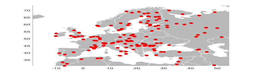
Figure 1: The distribution of the weather stations in the NOAA weather station dataset.

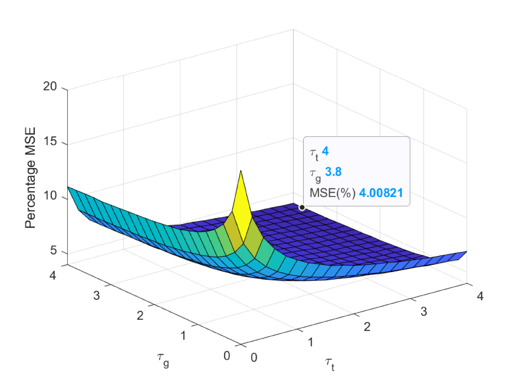
(a)

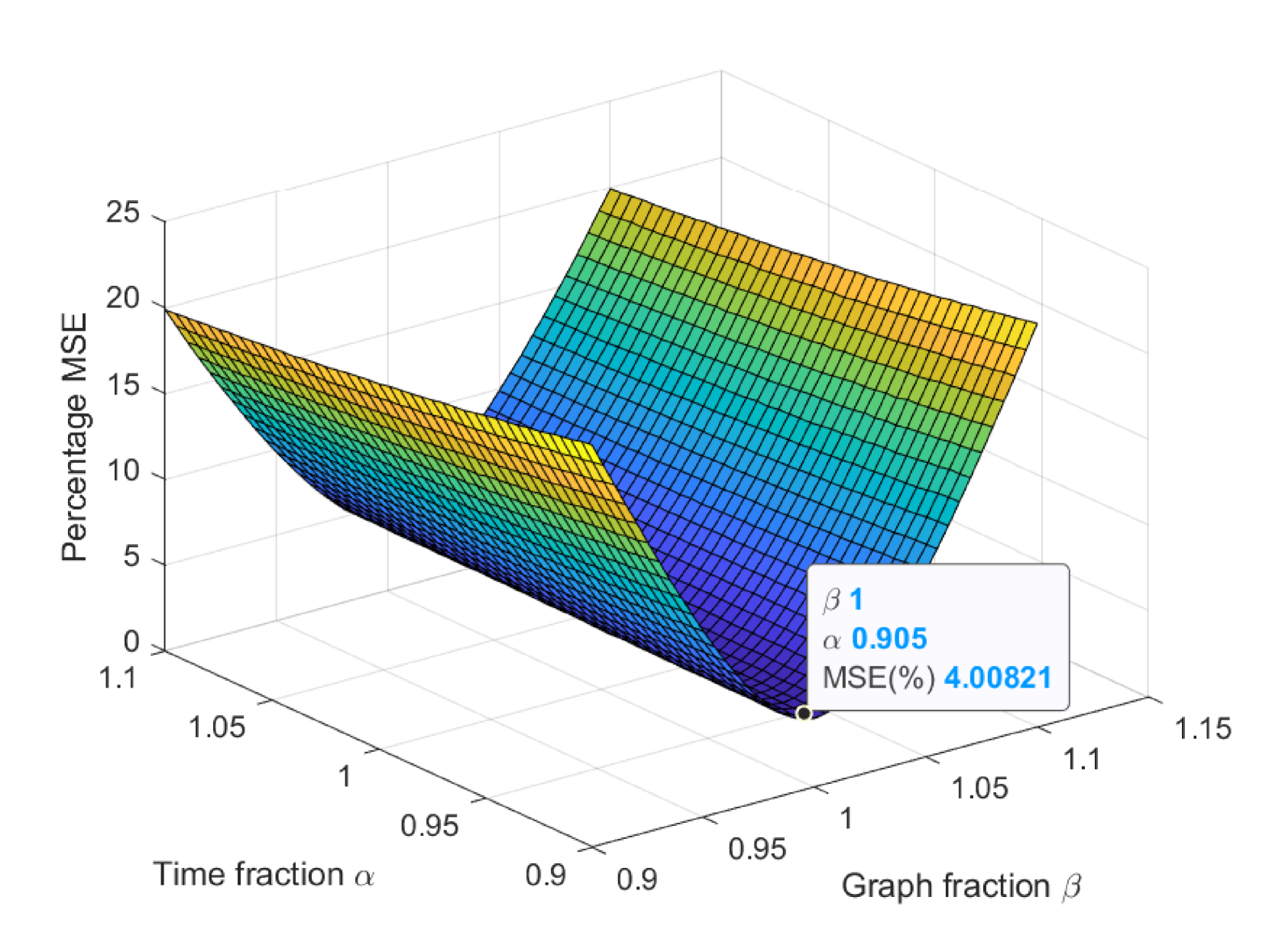
(b)

Figure 2: The results of the regularization based denoising applied to the Molene dataset. In (a) varying regularization parameters are considered while fractional orders are fixed to $\alpha=0.905$ and $\beta=1$, whereas in (b) fractional orders are considered with fixed regularization parameters $\tau_{g}=3.8,\tau_{t}=4$.

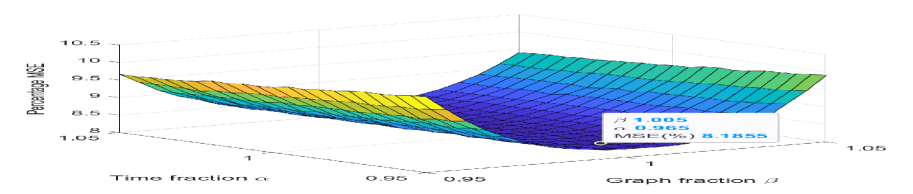
(a)

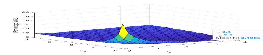
(b)

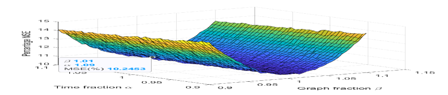
(c)

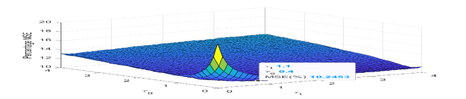
(d)

Figure 3: In the NOAA dataset, both yearly ((a), (b)) and monthly ((c), (d)) settings are considered. (a) shows the performance of denoising with respect to varying fractional orders with fixed regularization parameters $\tau_{t}=3.4$ and $\tau_{g}=0.4$. (b) shows the performance of varying regularization parameters with fixed JFRT orders ($\alpha=0.965,\beta=1.005$). Similarly, (c) shows the performance of varying fractional orders with $\tau_{t}=1.1,\tau_{g}=0.4$ and (d) shows the performance of regularization parameters with fixed ($\alpha=1.09,\beta=1.01$).

V-B Clustering Experiments

For this experiment, we consider the motions of the Dancer mesh, which consists of 1,502 coordinates in 3-dimensional space along 573 time samples [25]. These motions are moving arms, stretching legs and bending body motions. 2D plots of some actions taken from the dancer mesh dataset can be seen in Fig. 4 as examples. We followed the experimental procedure [25] provided to demonstrate the performance and utility of JFT, and extended it to conduct the clustering experiment for the proposed JFRT. The mesh is corrupted with additive sparse noise density 0.1, meaning that approximately 10% of mesh points are corrupted. The noise is Gaussian noise with signal-to-noise ratio (SNR) of -10 dB and -20 dB as in [25]. Rectangular windows of size 50 with 60$\%$ overlap are used to obtain 27 time sequences (The last 3 time samples are clipped). To capture the geometry of the data, a nearest neighbor graph is used.

We calculate JFRTs of the obtained sequences in each of the coordinate dimension, concatenate the resulting fractional order joint time-vertex signals, and finally cluster the resulting representation to get the classifications by using the k-means clustering algorithm. The experiment is repeated 20 times and Matlab rng seed of 1 is used. The results for the average accuracy of different JFRT orders for -10 and -20 dB SNR are presented in Fig. 5(a) and 5(b), respectively. It can be observed that the highest accuracy levels are achieved at fractional orders for both cases, indicating the performance improvements over the special case of the ordinary JFT. To make further comparisons, we also considered the cases of the ordinary JFT, the best obtained average accuracy of the (time-ordinary)/(graph-fractional) Fourier transform (JFRTg), the best obtained average accuracy of the (graph-ordinary)/(time-fractional) Fourier transform (JFRTt), the best obtained average accuracy for arbitrary JFRT and the received mesh (signal) without any transformation. JFRTg and JFRTt are the cases when we let only the graph order to be fractional and let only the time order to be fractional, respectively. This experiment is also repeated for 20 times and the results for -10 dB SNR and -20 dB SNR in box-plots are provided in Fig. 6(a) and 6(b), respectively. For both noise levels, distribution of accuracy is more confined to higher percentages at fractional orders. This shows that JFRT provides better clustering performance as the mesh points of similar motions are more densely populated in fractional domains.

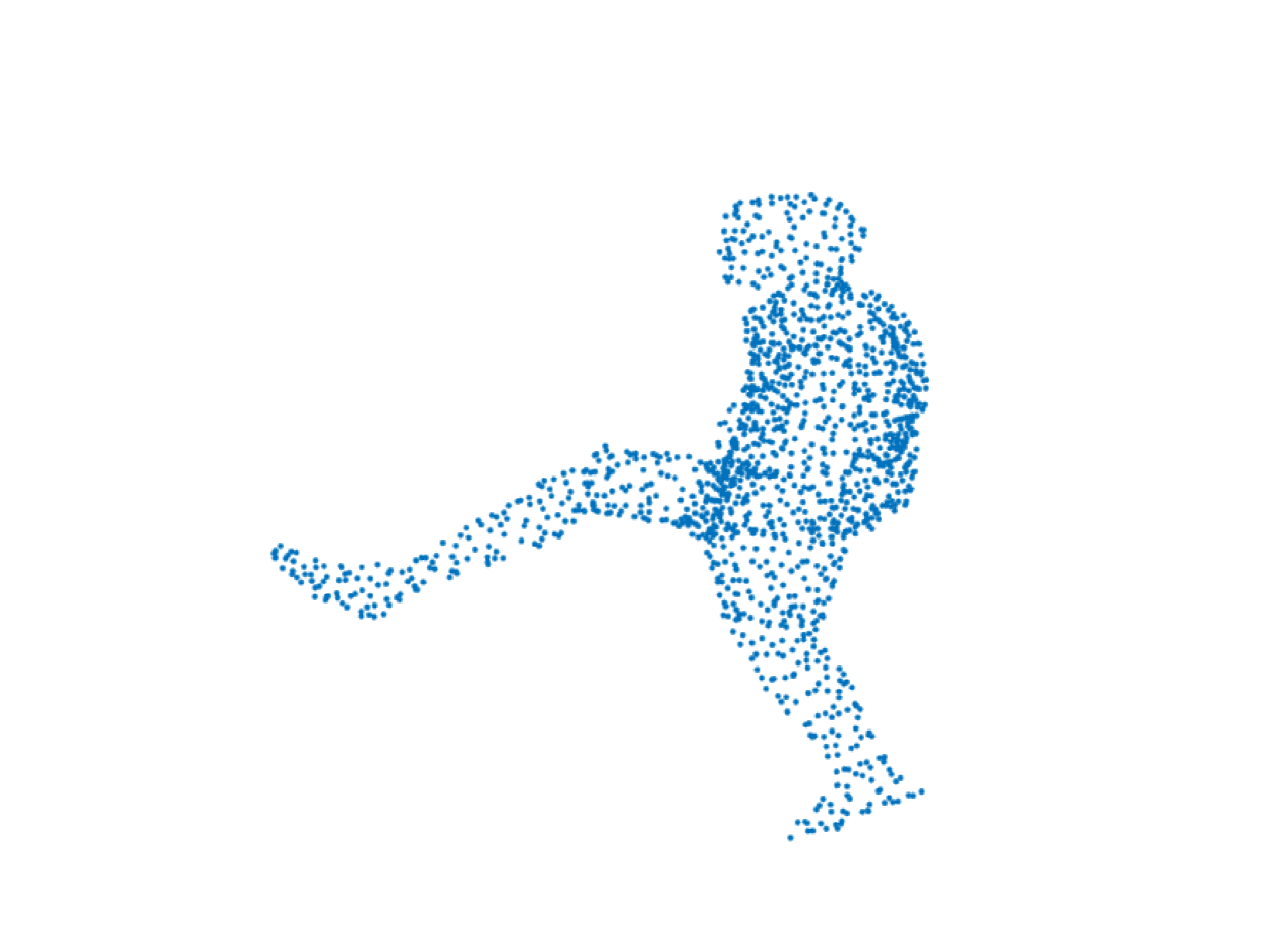
(a)

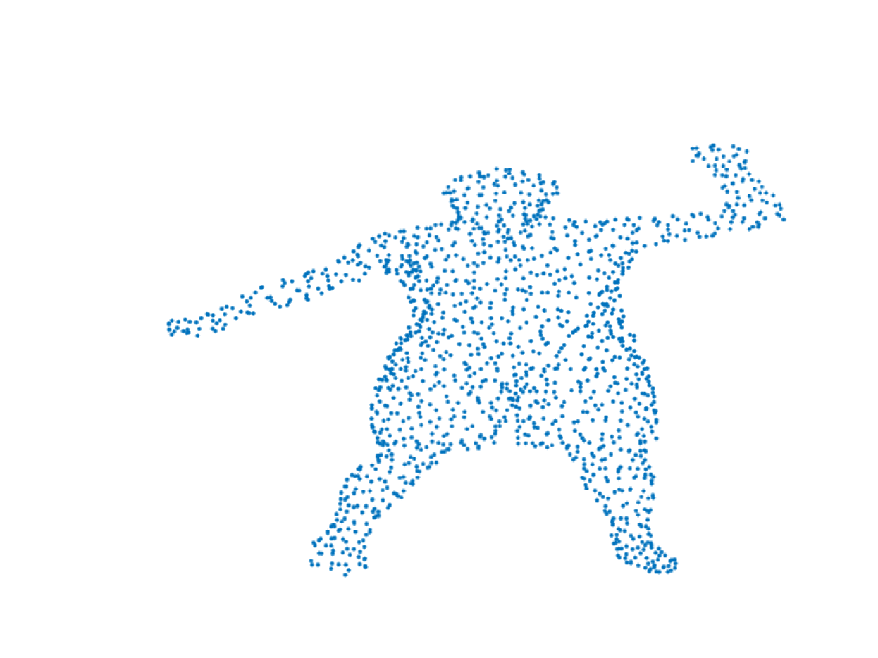
(b)

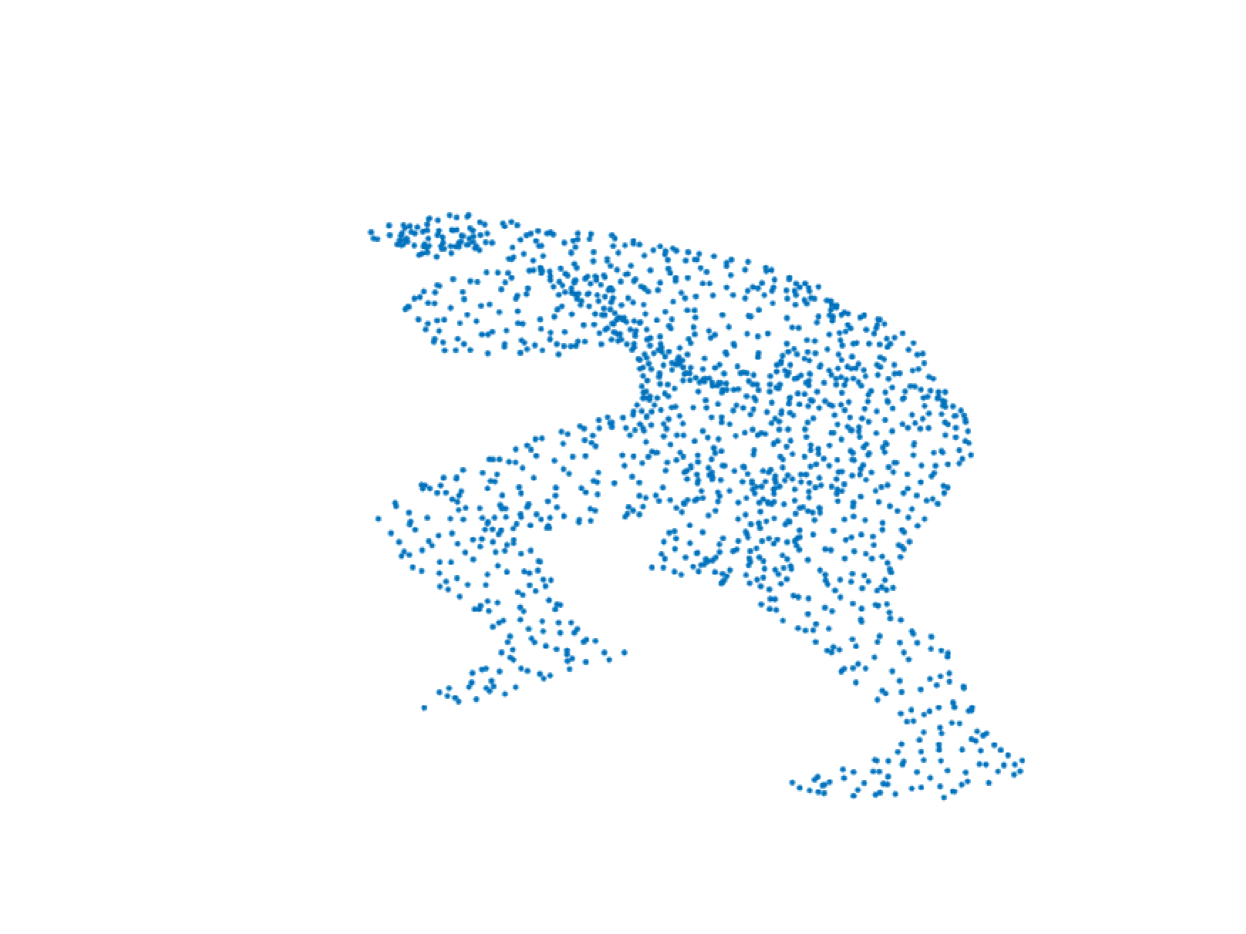
(c)

Figure 4: Sample frames from the actions of the Dancer mesh. (a) stretching legs; (b) moving arms; (c) bending body.

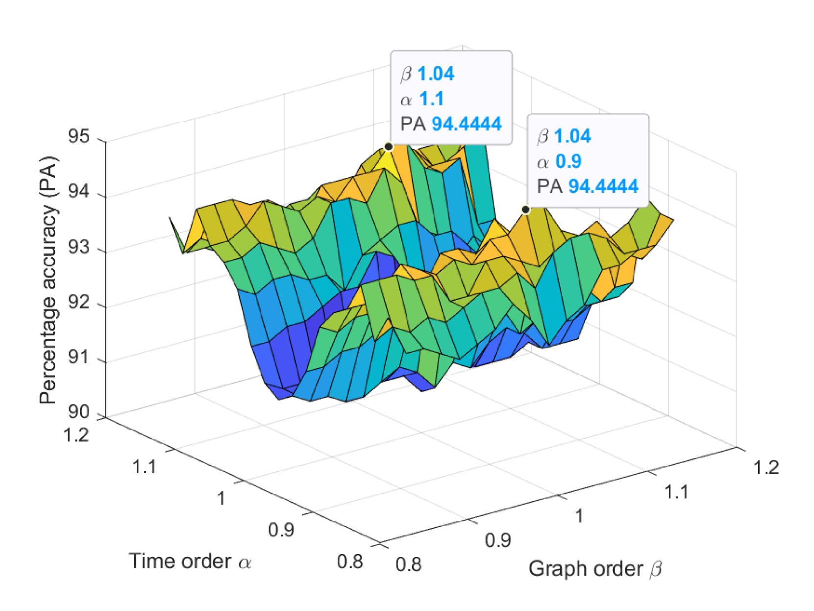
(a)

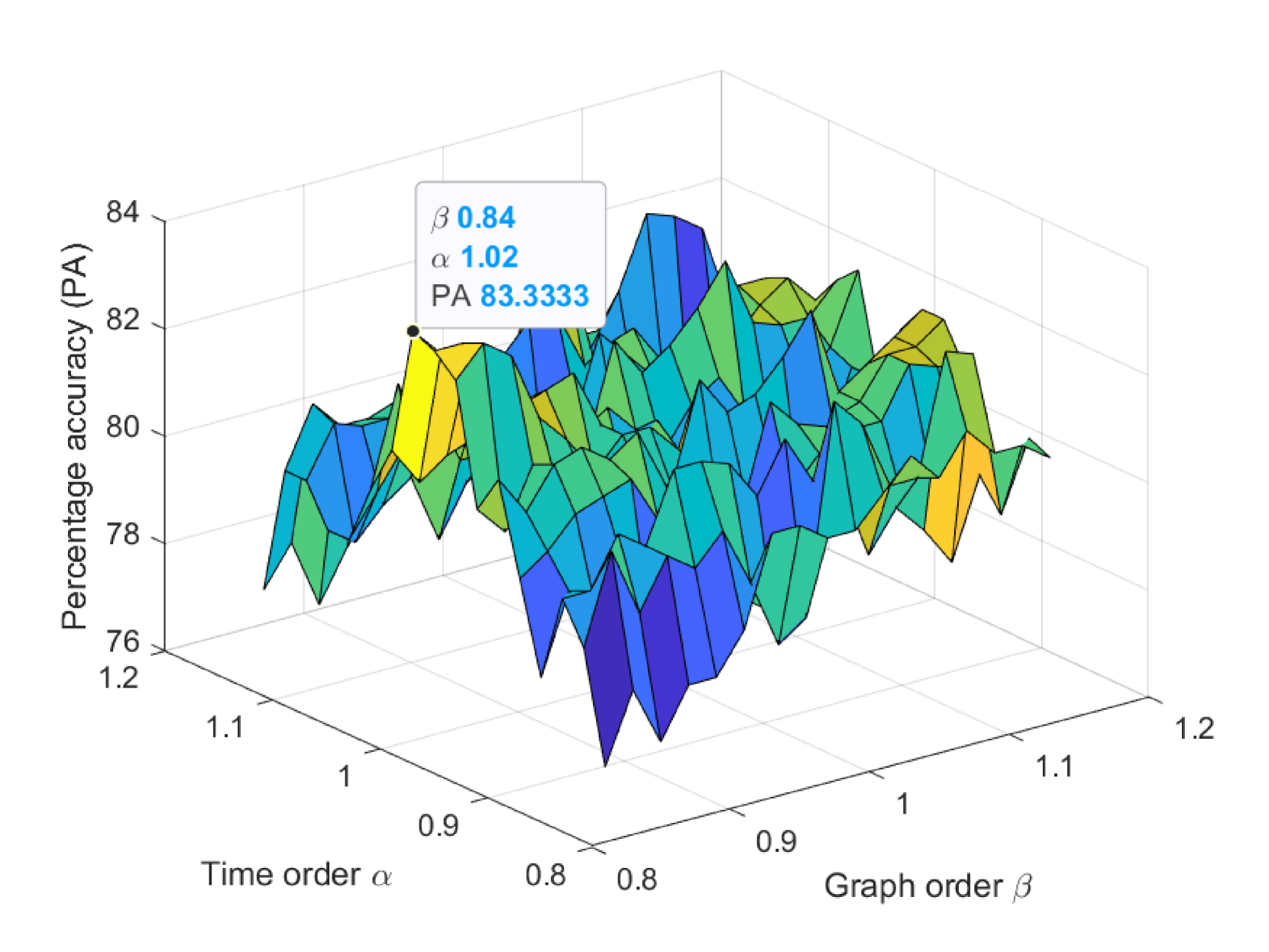
(b)

Figure 5: Performance of clustering accuracy for varying JFRT with (a) -10 dB SNR and (b) -20 dB SNR.

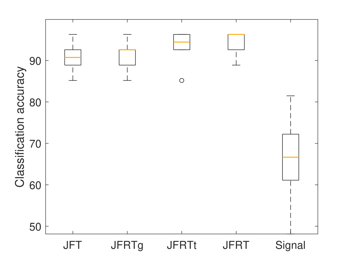
(a)

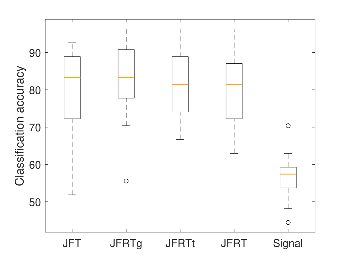
(b)

Figure 6: Box plots for the clustering performance of 20 samples for the ordinary JFT, the (time-ordinary)/(graph-fractional) Fourier transform (JFRTg), (graph-ordinary)/(time-fractional) Fourier transform (JFRTt), JFRT, and signal with (a) -10dB SNR and (b) -20 dB SNR.

VI Conclusion

We proposed the JFRT, a fractional transformation for processing joint time-vertex signals as a generalization to the ordinary JFT and two dimensional DFRT. With JFRT, it is possible to jointly transform time-varying graph signals into domains between vertex and graph-spectral domains from the graph perspective, and between time and frequency domains from the ordinary time-series perspective. Thus, JFRT could be seen as a transformation for two dimensional joint time-vertex signals. We showed that the proposed JFRT is index additive in orders, reversible and commutative. We also showed that the JFRT is unitary if the underlying GFT is unitary. JFRT reduces to the ordinary JFT when the order is $(1,1)$, reduces to the identity when the order is $(0,0)$, and, for directed circular graphs, reduces to the ordinary two dimensional DFRT for the order $(1,1)$. This makes JFT, 2D DFRT and 2D-DFT special cases of the JFRT.

We also constructed Tikhonov regularization-based denoising in the proposed JFRT domains by using the joint fractional Laplacian to regularize a received signal in both fractional time and fractional graph domains separately. We derived the associated optimal filter coefficients to be used in denoising.

The extra flexibility that the JFRT provides through its two parameters without imposing additional computational costs can open up several performance increases over the non-parametric JFT in joint time-vertex signal processing. We provided numerical examples in denoising and clustering tasks such that JFRT allows us to improve performance. As JFRT provides a new and flexible framework to handle joint-time vertex data, we expect that it will be instrumental for several signal processing applications as well as opening up new theoretical research directions in the joint time-vertex GSP. On the other side of the coin, we also extended the literature of FRT and contributed to the generalizations from the classical FRT analysis to the GSP domain by introducing JFRT.

References

- [1] A. Sandryhaila and J. M. F. Moura, “Discrete signal processing on graphs,” IEEE Transactions on Signal Processing, vol. 61, no. 7, pp. 1644–1656, April 2013.
- [2] D. I. Shuman, S. K. Narang, P. Frossard, A. Ortega, and P. Vandergheynst, “The emerging field of signal processing on graphs: Extending high-dimensional data analysis to networks and other irregular domains,” IEEE Signal Processing Magazine, vol. 30, no. 3, pp. 83–98, May 2013.
- [3] A. Sandryhaila and J. M. F. Moura, “Discrete signal processing on graphs: Graph filters,” in 2013 IEEE International Conference on Acoustics, Speech and Signal Processing, May 2013, pp. 6163–6166.
- [4] A. Sandryhaila and J. M. F. Moura, “Big data analysis with signal processing on graphs: Representation and processing of massive data sets with irregular structure,” IEEE Signal Processing Magazine, vol. 31, no. 5, pp. 80–90, Sep. 2014.
- [5] A. Sandryhaila and J. M. F. Moura, “Discrete signal processing on graphs: Frequency analysis,” IEEE Transactions on Signal Processing, vol. 62, no. 12, pp. 3042–3054, June 2014.
- [6] S. Chen, R. Varma, A. Sandryhaila, and J. Kovačević, “Discrete signal processing on graphs: Sampling theory,” IEEE Transactions on Signal Processing, vol. 63, no. 24, pp. 6510–6523, Dec 2015.
- [7] A. Gavili and X. Zhang, “On the shift operator, graph frequency, and optimal filtering in graph signal processing,” IEEE Transactions on Signal Processing, vol. 65, no. 23, pp. 6303–6318, Dec 2017.
- [8] Y. Wang, B. Li, and Q. Cheng, “The fractional Fourier transform on graphs,” in 2017 Asia-Pacific Signal and Information Processing Association Annual Summit and Conference (APSIPA ASC), Dec 2017, pp. 105–110.
- [9] G. Ribeiro and J. Lima, “Graph signal processing in a nutshell,” Journal of Communication and Information Systems, vol. 33, pp. 219–233, 01 2018.
- [10] A. Ortega, P. Frossard, J. Kovačević, J. M. F. Moura, and P. Vandergheynst, “Graph signal processing: Overview, challenges, and applications,” Proceedings of the IEEE, vol. 106, no. 5, pp. 808–828, May 2018.
- [11] Y. Wang and B. Li, “The fractional Fourier transform on graphs: Sampling and recovery,” 2018 14th IEEE International Conference on Signal Processing (ICSP), pp. 1103–1108, 2018.
- [12] L. Stanković, D. P. Mandic, M. Daković, M. Brajović, B. S. Dees, and T. Constantinides, “Graph signal processing - Part I: Graphs, graph spectra, and spectral clustering,” arXiv preprint arXiv:1907.03467 [cs.IT], 2019.
- [13] L. Stanković, D. Mandic, M. Daković, M. Brajović, B. Scalzo Dees, and A. Constantinides, “Graph signal processing – Part II: Processing and analyzing signals on graphs,” arXiv preprint arXiv:1909.10325 [cs.IT], 2019.
- [14] L. Stanković, D. Mandic, M. Daković, B. Scalzo, M. Brajović, E. Sejdić, and A. G. Constantinides, “Vertex-frequency graph signal processing: A comprehensive review,” Digital Signal Processing, vol. 107, p. 102802, 2020.
- [15] A. Anis, A. Gadde, and A. Ortega, “Towards a sampling theorem for signals on arbitrary graphs,” in 2014 IEEE International Conference on Acoustics, Speech and Signal Processing (ICASSP). IEEE, 2014, pp. 3864–3868.
- [16] S. K. Narang, A. Gadde, and A. Ortega, “Signal processing techniques for interpolation in graph structured data,” in 2013 IEEE International Conference on Acoustics, Speech and Signal Processing (ICASSP). IEEE, 2013, pp. 5445–5449.
- [17] X. Zhu and M. Rabbat, “Approximating signals supported on graphs,” in 2012 IEEE International Conference on Acoustics, Speech and Signal Processing (ICASSP), 2012, pp. 3921–3924.
- [18] J. Liu, E. Isufi, and G. Leus, “Filter design for autoregressive moving average graph filters,” IEEE Transactions on Signal and Information Processing over Networks, vol. 5, no. 1, pp. 47–60, 2019.
- [19] M. Onuki, S. Ono, M. Yamagishi, and Y. Tanaka, “Graph signal denoising via trilateral filter on graph spectral domain,” IEEE Transactions on Signal and Information Processing over Networks, vol. 2, no. 2, pp. 137–148, 2016.
- [20] F. Hua, C. Richard, J. Chen, H. Wang, P. Borgnat, and P. Gonçalves, “Learning combination of graph filters for graph signal modeling,” IEEE Signal Processing Letters, vol. 26, no. 12, pp. 1912–1916, 2019.
- [21] N. Saito, “How can we naturally order and organize graph Laplacian eigenvectors?” in 2018 IEEE Statistical Signal Processing Workshop (SSP), 2018, pp. 483–487.
- [22] M. Cheung, J. Shi, O. Wright, L. Y. Jiang, X. Liu, and J. M. F. Moura, “Graph signal processing and deep learning: Convolution, pooling, and topology,” IEEE Signal Processing Magazine, vol. 37, no. 6, pp. 139–149, 2020.
- [23] G. Leus, S. Segarra, A. Ribeiro, and A. G. Marques, “The dual graph shift operator: Identifying the support of the frequency domain,” Journal of Fourier Analysis and Applications, vol. 27, no. 49, 2021.
- [24] B. Kartal, Y. E. Bayiz, and A. Koç, “Graph signal processing: Vertex multiplication,” IEEE Signal Processing Letters, vol. 28, pp. 1270–1274, 2021.
- [25] F. Grassi, A. Loukas, N. Perraudin, and B. Ricaud, “A time-vertex signal processing framework: Scalable processing and meaningful representations for time-series on graphs,” IEEE Transactions on Signal Processing, vol. 66, no. 3, pp. 817–829, 2018.
- [26] F. Zhang and E. R. Hancock, “Graph spectral image smoothing using the heat kernel,” Pattern Recognition, vol. 41, no. 11, pp. 3328–3342, 2008.
- [27] D. I. Shuman, P. Vandergheynst, and P. Frossard, “Chebyshev polynomial approximation for distributed signal processing,” in 2011 International Conference on Distributed Computing in Sensor Systems and Workshops (DCOSS), 2011, pp. 1–8.
- [28] A. Loukas, M. Zuniga, M. Woehrle, M. Cattani, and K. Langendoen, “Think globally, act locally: On the reshaping of information landscapes,” in 2013 ACM/IEEE International Conference on Information Processing in Sensor Networks (IPSN), 2013, pp. 265–276.
- [29] A. C. Yagan and M. T. Ozgen, “Spectral graph based vertex-frequency Wiener filtering for image and graph signal denoising,” IEEE Transactions on Signal and Information Processing over Networks, vol. 6, pp. 226–240, 2020.
- [30] A. Loukas, M. Zuniga, I. Protonotarios, and J. Gao, “How to identify global trends from local decisions? Event region detection on mobile networks,” in IEEE Conference on Computer Communications (INFOCOM, 2014, pp. 1177–1185.
- [31] A. Smola and R. Kondor, “Kernels and regularization on graphs,” COLT/Kernel 2003, LNAI 2777, vol. 2777, pp. 144–158, 01 2003.
- [32] X. Zhu, Z. Ghahramani, and J. Lafferty, “Semi-supervised learning using Gaussian fields and harmonic functions.” in 20th International Conference on Machine Learning (ICML), vol. 3, 01 2003, pp. 912–919.
- [33] M. Belkin and P. Niyogi, “Laplacian eigenmaps and spectral techniques for embedding and clustering,” Advances in Neural Information Processing System, vol. 14, 04 2002.
- [34] H. P. Maretic and P. Frossard, “Graph Laplacian mixture model,” IEEE Transactions on Signal and Information Processing over Networks, vol. 6, pp. 261–270, 2020.
- [35] N. Shahid, N. Perraudin, V. Kalofolias, G. Puy, and P. Vandergheynst, “Fast robust PCA on graphs,” IEEE Journal of Selected Topics in Signal Processing, vol. 10, no. 4, p. 740–756, Jun 2016.
- [36] N. Perraudin and P. Vandergheynst, “Stationary signal processing on graphs,” IEEE Transactions on Signal Processing, vol. 65, no. 13, pp. 3462–3477, 2017.
- [37] A. G. Marques, S. Segarra, G. Leus, and A. Ribeiro, “Stationary graph processes and spectral estimation,” IEEE Transactions on Signal Processing, vol. 65, no. 22, pp. 5911–5926, 2017.
- [38] D. K. Hammond, P. Vandergheynst, and R. Gribonval, “Wavelets on graphs via spectral graph theory,” Applied and Computational Harmonic Analysis, vol. 30, no. 2, pp. 129 – 150, 2011.
- [39] R. R. Coifman and M. Maggioni, “Diffusion wavelets,” Applied and Computational Harmonic Analysis, vol. 21, no. 1, pp. 53 – 94, 2006, special Issue: Diffusion Maps and Wavelets.
- [40] M. Belkin and P. Niyogi, “Semi-supervised learning on Riemannian manifolds: Theoretical advances in data clustering (guest editors: Nina Mishra and Rajeev Motwani),” Machine Learning, vol. 56, 07 2004.
- [41] X. Zheng, Y. Y. Tang, J. Pan, and J. Zhou, “Adaptive multiscale decomposition of graph signals,” IEEE Signal Processing Letters, vol. 23, no. 10, pp. 1389–1393, 2016.
- [42] S. K. Narang and A. Ortega, “Perfect reconstruction two-channel wavelet filter banks for graph structured data,” IEEE Transactions on Signal Processing, vol. 60, no. 6, pp. 2786–2799, 2012.
- [43] A. Sakiyama, K. Watanabe, and Y. Tanaka, “Spectral graph wavelets and filter banks with low approximation error,” IEEE Transactions on Signal and Information Processing over Networks, vol. 2, no. 3, pp. 230–245, 2016.
- [44] S. Kwak, N. Geroliminis, and P. Frossard, “Traffic signal prediction on transportation networks using spatio-temporal correlations on graphs,” IEEE Transactions on Signal and Information Processing over Networks, vol. 7, pp. 648–659, 2021.
- [45] E. Bayram, D. Thanou, E. Vural, and P. Frossard, “Mask combination of multi-layer graphs for global structure inference,” IEEE Transactions on Signal and Information Processing over Networks, vol. 6, pp. 394–406, 2020.
- [46] H. E. Egilmez, E. Pavez, and A. Ortega, “Graph learning from filtered signals: Graph system and diffusion kernel identification,” IEEE Transactions on Signal and Information Processing over Networks, vol. 5, no. 2, pp. 360–374, 2019.
- [47] J. Yang, S. C. Draper, and R. Nowak, “Learning the interference graph of a wireless network,” IEEE Transactions on Signal and Information Processing over Networks, vol. 3, no. 3, pp. 631–646, 2017.
- [48] H. Sadreazami, A. Mohammadi, A. Asif, and K. N. Plataniotis, “Distributed-graph-based statistical approach for intrusion detection in cyber-physical systems,” IEEE Transactions on Signal and Information Processing over Networks, vol. 4, no. 1, pp. 137–147, 2018.
- [49] L. Stanković, D. Mandic, M. Daković, M. Brajović, B. Scalzo, S. Li, and A. G. Constantinides, “Graph signal processing – Part III: Machine learning on graphs, from graph topology to applications,” arXiv preprint arXiv:2001.00426 [cs.IT], 2020.
- [50] M. Ye, V. Stankovic, L. Stankovic, and G. Cheung, “Robust deep graph based learning for binary classification,” IEEE Transactions on Signal and Information Processing over Networks, vol. 7, pp. 322–335, 2021.
- [51] P. Berger, G. Hannak, and G. Matz, “Efficient graph learning from noisy and incomplete data,” IEEE Transactions on Signal and Information Processing over Networks, vol. 6, pp. 105–119, 2020.
- [52] Y. Shen, W. Dai, C. Li, J. Zou, and H. Xiong, “Multi-scale graph convolutional network with spectral graph wavelet frame,” IEEE Transactions on Signal and Information Processing over Networks, vol. 7, pp. 595–610, 2021.
- [53] A. Loukas and D. Foucard, “Frequency analysis of time-varying graph signals,” in 2016 IEEE Global Conference on Signal and Information Processing (GlobalSIP), 2016, pp. 346–350.
- [54] N. Perraudin, A. Loukas, F. Grassi, and P. Vandergheynst, “Towards stationary time-vertex signal processing,” in 2017 IEEE International Conference on Acoustics, Speech and Signal Processing (ICASSP), 2017, pp. 3914–3918.
- [55] A. Loukas and N. Perraudin, “Stationary time-vertex signal processing,” EURASIP Journal on Advances in Signal Processing, vol. 2019, no. 1, p. 36, Aug 2019.
- [56] E. Isufi, A. Loukas, A. Simonetto, and G. Leus, “Autoregressive moving average graph filtering,” IEEE Transactions on Signal Processing, vol. 65, no. 2, pp. 274–288, 2017.
- [57] E. Isufi, A. Loukas, N. Perraudin, and G. Leus, “Forecasting time series with VARMA recursions on graphs,” IEEE Transactions on Signal Processing, vol. 67, no. 18, pp. 4870–4885, 2019.
- [58] K. Qiu, X. Mao, X. Shen, X. Wang, T. Li, and Y. Gu, “Time-varying graph signal reconstruction,” IEEE Journal of Selected Topics in Signal Processing, vol. 11, no. 6, pp. 870–883, 2017.
- [59] X. Mao and Y. Gu, Time-Varying Graph Signals Reconstruction. Cham: Springer International Publishing, 2019, pp. 293–316.
- [60] J. H. Giraldo and T. Bouwmans, “On the minimization of Sobolev norms of time-varying graph signals: Estimation of new coronavirus disease 2019 cases,” in 2020 IEEE 30th International Workshop on Machine Learning for Signal Processing (MLSP), 2020, pp. 1–6.
- [61] A. Loukas, E. Isufi, and N. Perraudin, “Predicting the evolution of stationary graph signals,” in 2017 51st Asilomar Conference on Signals, Systems, and Computers, 2017, pp. 60–64.
- [62] C. Pan, S. Chen, and A. Ortega, “Spatio-temporal graph scattering transform,” in International Conference on Learning Representations, 2021.
- [63] P. Das and A. Ortega, “Symmetric sub-graph spatio-temporal graph convolution and its application in complex activity recognition,” in ICASSP 2021 - 2021 IEEE International Conference on Acoustics, Speech and Signal Processing (ICASSP), 2021, pp. 3215–3219.
- [64] H. M. Ozaktas and D. Mendlovic, “Fourier transforms of fractional order and their optical interpretation,” Optics Communications, vol. 101, no. 3-4, pp. 163–169, 1993.
- [65] D. Mendlovic and H. M. Ozaktas, “Fractional Fourier transforms and their optical implementation: I,” J. Opt. Soc. Am. A, vol. 10, pp. 1875–1881, 1993.
- [66] H. M. Ozaktas and D. Mendlovic, “Fractional Fourier transforms and their optical implementation: II,” J. Opt. Soc. Am. A, vol. 10, pp. 2522–2531, 1993.
- [67] H. M. Ozaktas, Z. Zalevsky, and M. A. Kutay, The Fractional Fourier Transform with Applications in Optics and Signal Processing. New York: Wiley, 2001.
- [68] S. C. Pei and J. J. Ding, “Closed-form discrete fractional and affine Fourier transforms,” IEEE Transactions on Signal Processing, vol. 48, pp. 1338–1353, 2000.
- [69] L. B. Almeida, “The fractional Fourier transform and time-frequency representations,” IEEE Transactions on Signal Processing, vol. 42, pp. 3084–3091, 1994.
- [70] H. M. Ozaktas, M. A. Kutay, and C. Candan, Transforms and Applications Handbook. New York, NY: CRC Press, Boca Raton, 2010, ch. Fractional Fourier Transform, pp. 14–1–14–28.
- [71] A. I. Zayed and A. G. Garcia, “New sampling formulae for the fractional Fourier transform,” Signal Processing, vol. 77, no. 1, pp. 111 – 114, 1999.
- [72] D. Mustard, “The fractional Fourier transform and the Wigner distribution,” The Journal of the Australian Mathematical Society. Series B. Applied Mathematics, vol. 38, no. 2, p. 209–219, 1996.
- [73] M. A. Kutay, H. M. Ozaktas, L. Onural, and O. Arikan, “Optimal filtering in fractional Fourier domains,” in 1995 International Conference on Acoustics, Speech, and Signal Processing, vol. 2, May 1995, pp. 937–940 vol.2.
- [74] M. A. Kutay, H. M. Ozaktas, O. Arikan, and L. Onural, “Optimal filtering in fractional Fourier domains,” IEEE Transactions on Signal Processing, vol. 45, pp. 1129–1143, 1997.
- [75] Z. Zalevsky and D. Mendlovic, “Fractional Wiener filter,” Appl. Opt., vol. 35, no. 20, pp. 3930–3936, Jul 1996.
- [76] P. Muralidhar, S. Nayak, and T. Sahu, “Implementation of fractional Fourier transform in digital filter design,” Journal of Communications, pp. 289–302, 01 2020.
- [77] A. W. Lohmann, “Image rotation, Wigner rotation, and the fractional Fourier transform,” J. Opt. Soc. Am. A, vol. 10, no. 10, pp. 2181–2186, 1993.
- [78] K. K. Sharma and M. Sharma, “Image fusion based on image decomposition using self-fractional Fourier functions,” Signal, Image and Video Process., vol. 8, no. 7, pp. 1335–1344, Oct 2014.
- [79] N. Jindal and K. Singh, “Image and video processing using discrete fractional transforms,” Signal, Image and Video Process., vol. 8, no. 8, pp. 1543–1553, Nov 2014.
- [80] M. I. Ahmad, M. U. Sardar, and I. Ahmad, “Blind beamforming using fractional Fourier transform domain cyclostationarity,” Signal, Image and Video Process., vol. 12, no. 2, pp. 379–383, Feb 2018.
- [81] M. I. Ahmad, “Optimum FrFT domain cyclostationarity based adaptive beamforming,” Signal, Image and Video Process., vol. 13, no. 3, pp. 551–556, Apr 2019.
- [82] D. Mendlovic, Z. Zalevsky, and H. M. Ozaktas, Optical Pattern Recognition. New York, NY: New York Academic, 1998, ch. The applications of the fractional Fourier transform to optical pattern recognition.
- [83] B.-Z. Dong, Y. Zhang, B.-Y. Gu, and G.-Z. Yang, “Numerical investigation of phase retrieval in a fractional Fourier transform,” J. Opt. Soc. Am. A, vol. 14, no. 10, pp. 2709–2714, Oct 1997.
- [84] R. Jacob, T. Thomas, and A. Unnikrishnan, “Applications of fractional Fourier transform in sonar signal processing,” IETE J. of Res., vol. 55, no. 1, pp. 16–27, 2009.
- [85] Z. Zhao, R. Tao, G. Li, and Y. Wang, “Fractional sparse energy representation method for ISAR imaging,” IET Radar, Sonar Navigation, vol. 12, no. 9, pp. 988–997, 2018.
- [86] F.-J. Yan, W.-B. Gao, and B.-Z. Li, “Windowed fractional Fourier transform on graphs: Fractional translation operator and hausdorff-young inequality,” in 2020 Asia-Pacific Signal and Information Processing Association Annual Summit and Conference (APSIPA ASC), 2020, pp. 255–259.
- [87] F.-J. Yan and B.-Z. Li, “Windowed fractional Fourier transform on graphs: Properties and fast algorithm,” Digital Signal Processing, vol. 118, p. 103210, 2021.
- [88] J. Wu, F. Wu, Q. Yang, Y. Zhang, X. Liu, Y. Kong, L. Senhadji, and H. Shu, “Fractional spectral graph wavelets and their applications,” Mathematical Problems in Engineering, 2020.
- [89] F.-J. Yan and B.-Z. Li, “Multi-dimensional graph fractional Fourier transform and its application,” 2021.
- [90] C. Ozturk, H. M. Ozaktas, S. Gezici, and A. Koç, “Optimal fractional Fourier filtering for graph signals,” IEEE Transactions on Signal Processing, vol. 69, pp. 2902–2912, 2021.
- [91] R. Shafipour, A. Khodabakhsh, G. Mateos, and E. Nikolova, “A directed graph Fourier transform with spread frequency components,” IEEE Transactions on Signal Processing, vol. 67, no. 4, pp. 946–960, 2019.
- [92] S. Furutani, T. Shibahara, M. Akiyama, K. Hato, and M. Aida, “Graph signal Processing for directed graphs based on the Hermitian Laplacian,” in Machine Learning and Knowledge Discovery in Databases, U. Brefeld, E. Fromont, A. Hotho, A. Knobbe, M. Maathuis, and C. Robardet, Eds. Cham: Springer International Publishing, 2020, pp. 447–463.
- [93] R. Singh, A. Chakraborty, and B. S. Manoj, “Graph Fourier transform based on directed Laplacian,” in 2016 International Conference on Signal Processing and Communications (SPCOM), 2016, pp. 1–5.
- [94] C. Candan, M. A. Kutay, and H. M. Ozaktas, “The discrete fractional Fourier transform,” IEEE Transactions on Signal Processing, vol. 48, no. 5, pp. 1329 –1337, 2000.
- [95] R. Shafipour, A. Khodabakhsh, G. Mateos, and E. Nikolova, “A digraph Fourier transform with spread frequency components,” in 2017 IEEE Global Conference on Signal and Information Processing (GlobalSIP), 2017, pp. 583–587.
- [96] H. M. Ozaktas, O. Arıkan, M. A. Kutay, and G. Bozdağı, “Digital computation of the fractional Fourier transform,” IEEE Transactions on Signal Processing, vol. 44, pp. 2141–2150, 1996.
- [97] L. Le Magoarou, R. Gribonval, and N. Tremblay, “Approximate fast graph Fourier transforms via multilayer sparse approximations,” IEEE Transactions on Signal and Information Processing over Networks, vol. 4, no. 2, pp. 407–420, 2018.
- [98] L. Le Magoarou and R. Gribonval, “Are there approximate fast Fourier transforms on graphs?” in 2016 IEEE International Conference on Acoustics, Speech and Signal Processing (ICASSP), 2016, pp. 4811–4815.
- [99] J. Domingos and J. M. F. Moura, “Graph Fourier transform: A stable approximation,” IEEE Transactions on Signal Processing, vol. 68, pp. 4422–4437, 2020.
- [100] K. Lu and A. Ortega, “Fast graph Fourier transforms based on graph symmetry and bipartition,” IEEE Transactions on Signal Processing, vol. 67, no. 18, pp. 4855–4869, 2019.
- [101] B. Girault, P. Gonçalves, and E. Fleury, “Translation on graphs: An isometric shift operator,” IEEE Signal Processing Letters, vol. 22, no. 12, pp. 2416–2420, 2015.