The REDTOP experiment: Rare $\eta/\eta^{\prime}$ Decays To Probe New Physics.

Abstract

The $\eta$ and $\eta^{\prime}$ mesons are nearly unique in the particle universe since they are almost Goldstone bosons and the dynamics of their decays are strongly constrained. The integrated $\eta$-meson samples collected in earlier experiments amount to $\sim 10^{9}$ events. A new experiment, REDTOP (Rare Eta Decays To Observe Physics Beyond the Standard Model), is being proposed, with the intent of collecting a data sample of order 10¹⁴ $\eta$ (10¹² $\eta^{\prime}$) for studying very rare decays. Such statistics are sufficient for investigating several symmetry violations, and for searching for particles and fields beyond the Standard Model. In this work we present several studies evaluating REDTOP sensitivity to processes that couple the Standard Model to New Physics through all four of the so-called portals: the Vector, the Scalar, the Axion and the Heavy Lepton portal. The sensitivity of the experiment is also adequate for probing several conservation laws, in particular $CP$, $T$ and Lepton Universality, and for the determination of the $\eta$ form factors, which is crucial for the interpretation of the recent measurement of muon $g-2$.
Preprint numbers: FERMILAB-FN-1153-AD-PPD-T, LA-UR-22-22208

REDTOP Collaboration Homepage: ]https://redtop.fnal.gov

Executive Summary

• The next decade represents an almost unique opportunity for laboratories with high intensity proton accelerators to uncover Dark Matter or New Physics.

• There are strong theoretical reasons to search for New Physics in the MeV–GeV range.

• The $\eta$ and $\eta^{\prime}$ mesons are almost unique since they carry he same quantum numbers as the Higgs (except for parity), and have no Standard Model charges. Their decays are flavor-conserving and most of them forbidden at leading order (in various symmetry-breaking parameters) within the Standard Model.

• Rare decays are therefore enhanced compared to the remaining flavor-neutral mesons. Thus an $\eta/\eta^{\prime}$ factory is an excellent laboratory for studying rare processes and Beyond Standard Model physics at low energy.

• A sample of order $10^{14}$($10^{12}$ ) $\eta(\eta^{\prime})$ mesons can address most of the recent theoretical models. Such an experiment would have enough sensitivity to explore a very large portion of the unexplored parameter space for all the four portals connecting the Dark Sector with the Standard Model. Lepton Universality and the $CP$ and $T$ symmetries can also be probed with excellent sensitivity.

• Many other studies can be conducted with such a large data sample, including, for example, the determination of the $\eta$ form factors, which is crucial to understanding the $(g-2)_{\mu}$ measurement.

• The REDTOP Collaboration is proposing an $\eta/\eta^{\prime}$ factory with such parameters. No similar experiment exists or is currently planned by the international community.

• A full detector simulation and reconstruction has been implemented to study several processes driven by New Physics, and many theoretical models have been bench marked. About $5\times 10{}^{10}$ background events have been generated and fully reconstructed to estimate the sensitivity of REDTOP. This took over three years to complete and required about $4\times 10{}^{7}$ core-hours of computing on the Open Science Grid.

• The Physics case for REDTOP is presented in the first part of this work. In Sec. III.1 we discuss the four portals and the latest theoretical models proposed to explain outstanding experimental anomalies. In Sec. III.2 we discuss several tests of conservation laws which could be explored at REDTOP.

• A description of the experiment, including the sub-detectors, the trigger systems and the computing model, is presented in the central part of this document. Radiation damage, detector aging and shielding issues have also been considered. They are discussed in some detail in the appendices.

I Introduction

It is generally accepted that the Standard Model (SM) is not a complete description of all quantum interactions. The exact nature of dark energy and dark matter, and the baryon asymmetry of the universe, the observation of a Universe in accelerating expansion, and neutrino masses, are among the very interesting questions that cannot be answered within the framework of the SM.

There is a strong indication that the physics Beyond the Standard Model (BSM) could contain new particles and/or force mediators, which significantly violate some discrete symmetries of the universe, in particular CP.

The High Energy Physics community has engaged in an unprecedented experimental effort, with the construction of the LHC and its four detectors, to observe physics BSM in the High Energy domain. The absence of conclusive evidence so far may suggest that: a) the New Physics most immediately accessible to experimenters is at low energies, rather than at high energies, and b) such New Physics is elusive, in particular it couples to SM matter too faintly to be detected by experiments at colliders. To detect such interactions, one may need huge luminosities, which are one of the most attractive features of fixed-target experiments.

As a consequence of fact a), a plethora of new theoretical models have flourished, that extend the SM with light gauge bosons, in the MeV–GeV mass range (see e.g., (Batell et al., 2009a; Reece and Wang, 2009; Bjorken et al., 2009)). Such efforts have, on the one hand, been encouraged by the fact that recently observed astrophysical anomalies point to such mass range as a promising area of exploration. In addition, in such mass regime, otherwise strong astrophysical and cosmological constraints are weakened or eliminated, while constraints from high energy colliders are, in most cases, inapplicable.

On the other side, fact b) puts the spotlight on experimental searches with techniques resting on an integrated luminosity that exceeds by several orders of magnitudes those currently available at colliders. As pointed out in Ref. Batell et al. (2009b), while the characteristic integrated luminosity for high-energy colliders is of order 10⁴¹cm^-2, the analogue of integrated luminosity for a moderate intensity (namely, $\sim$10²¹ protons on target (POT)) fixed target experiment with a 1 mm thick target is of the order of $\sim$10⁴⁴ cm^-2. By applying formula (4) in Ref. Batell et al. (2009b) at a fixed target experiment with E_lab=1 GeV, one obtains the following comparison between the production rates for neutral GeV-scale states at LHC and low energy fixed targets:

$$\frac{N_{LHC}}{N_{fixed\>target}}\sim 10^{-8+6n}$$ (1)

where the interaction between the standard and dark matter is assumed being mediated by marginal or irrelevant operators of dimension $4+n$, with $n\geq 0$.

For the kind of New Physics mentioned above, fixed-target experiments with hadronic beams thus have well-defined advantages with respect to high-energy colliders — let alone the tremendous difference in construction and operating costs. At the same time, several factors are limiting the realization of a high intensity fixed target experiment. Two of the most limiting factors are: a) the sheer production rate of events from inelastic interaction of the beam onto the target and, b) the large background from neutrons (either primary or secondary) which make a signal in the detector. Regarding point a), the technologies implemented in the present generation of detectors are not fast enough to cope with proton beam intensities even as modest as few tens of watts. Regarding point b), a neutron and a photon have very similar signatures in a conventional, single-readout calorimeter, hindering the ability to disentangle such particles unless novel detector techniques are implemented. Last, but not least, intense neutron fluxes could damage quickly a detector if non radiation-hard materials are used.

The design of the REDTOP experiment is based on the above considerations. REDTOP is a high yield $\eta$/$\eta^{\prime}$-factory, operated in a fixed target configuration with beam luminosity of order 10³⁴ cm^-2sec^-1. The mass range for potential discoveries is approximately [14 MeV-950 MeV], limited on the lower side by the resolution of the detector and on the upper side by the meson mass.

REDTOP is also a frontier experiment, aiming at measuring the $\eta/\eta^{\prime}$ decay rates or their asymmetries for very rare processes, and with a precision several orders of magnitude higher than the present measurements. These decays would provide direct tests of conservation laws and, along with other measurements, will open up new windows to discover physics beyond the Standard Model. In addition to searches for new physics, the experiment will involve development and first use of innovative detectors. Novel instrumentation will include a super-light  Frisch (2014) or an LGAD tracker with unprecedentedly low material budget et al. (2020), an ADRIANO2 calorimeter, and a Threshold Cerenkov Radiator (TCR). An optional Active Muon Polarimeter is being considered to improve the measurements of the muon polarization. With the information obtained from the highly granular calorimeter as well as from the other subdetectors, an extended Particle Flow Analysis (PFA) M.Thomson (2006) could be implemented. The 5-D measurement performed on the showers (energy, space, and time) will facilitate the disentangling of complex or overlapping events.

The development of all such detector techniques will require a substantial effort. On the other hand, future experiments, operating with similar event rates or requiring similar levels of background rejection, will certainly benefit from the pioneering R&D carried by the REDTOP Collaboration.

II Motivations for a high luminosity $\eta/\eta^{\prime}$ factory

It has been recently noted that “Light dark matter (LDM) must be neutral under SM charges, otherwise it would have been discovered at previous colliders” Krnjaic (2020). Under such circumstance, the study of processes originated by particles carrying no SM charges is, intuitively, more appropriate in LDM searches, as no charged currents are present, which could potentially interfere with Beyond Standard Model (BSM) processes.

The $\eta$ and $\eta^{\prime}$ mesons have been widely studied in the past, as their special nature has attracted the curiosity of the scientists (Nefkens, 1996). The $\eta$ is a Goldstone boson, therefore its QCD dynamics is strongly constrained by that property. In nature, there are only few Goldstone bosons. Furthermore, the $\eta$ is, at the same time, an eigenstate of the C, P, CP, I and G operators with all zero eigenvalues (namely: $I^{G}J^{PC}=0^{+}0^{-+}$) which makes it identical (except for parity) to the vacuum or the Higgs boson. In that respect, it is a very pure state, carrying no Standard Model charges and, as noted above, its decays do not involve charge-changing currents: all decays of $\eta$ and $\eta^{\prime}$ mesons are flavor-conserving. Therefore, a $\eta/\eta^{\prime}$-factory could be interpreted as a “low-energy Higgs-factory”, anticipating much of the exploration achievable at a high-energy Higgs factory. Any coupling to BSM states, therefore, does not interfere with Standard Model charge-changing operators (as it occurs, for example, with mesons carrying flavor). From the experimental point of view, the $\eta/\eta^{\prime}$ dynamics is particularly favorable to the exploration of small BSM effects since, as a consequence of the properties mentioned above, they have an unusually small decay width ($\Gamma_{\eta}$=1.3 KeV vs $\Gamma_{\rho}$=149 MeV, for example). Electromagnetic and strong decays are suppressed up to order $\mathcal{O}(10^{-6})$ favoring the study of more rare decays, especially those related to BSM particles and to violation of discrete symmetries. This helps considerably in reconstructing the kinematic of the event and in reducing the Standard Model background by requiring that the invariant mass of the final state particles is consistent with the $\eta$ mass.

Another reason to investigate more precisely the $\eta/\eta^{\prime}$ mesons is that their structure has never been fully understood. Recent work Singh and Patel (2011) indicates that such mesons are unique among the pseudoscalars as they have anomalously large masses which are contributed by quarks only about 80% of the momentum, leaving considerable room for potential contribution by New Physics.

A summary of the processes that can be studied at REDTOP for exploring New Physics is shown in Fig. 1. The processes are grouped by their physics topic, and will be discussed in more details in the next sections.

Figure 1: Physics landscape for a $\eta/\eta^{\prime}$ factory.

Considering the present limits on the parameters associated to BSM physics and the practical limitations of current detector technologies, the next generation of experiments should be designed with the goal of producing no less than $10^{13}$ $\eta$ mesons and $10^{11}$ $\eta^{\prime}$ mesons. The physics reach of an experiment with such statistics is very broad, spanning several aspects of physics BSM. The most relevant processes to be explored fall into two main fields of research: Search for New Particle and Fields, and Test of Conservation laws. Along with BSM Physics, the availability of such a large sample of flavor-conserving mesons will also allow probing the isospin violating sector of low energy QCD to an unprecedented degree of precision. The large number of processes that could be studied at the proposed $\eta/\eta^{\prime}$-factory will provide not only a nice scientific laboratory but also the source of many topics for Ph.D. thesis.

Few of the BSM processes accessible with an $\eta/\eta^{\prime}$-factory of REDTOP class have been selected for detailed sensitivity studies. They will be discussed later in this paper, along with several recent theoretical models which are explaining some of the anomalies that have been observed by the experiments.

III BSM physics with an $\eta/\eta^{\prime}$ factory

Large samples of $\eta/\eta^{\prime}$ decays open new avenues for the study of BSM physics. This is particularly true for weakly coupled hidden sectors, in which the new fields are SM singlets, as well as studies of fundamental symmetries and their breaking.

Models of new hidden sectors are typified by so-called portals, in which a new field, either a vector, scalar, or a heavy neutral lepton, appears in an SM gauge-singlet interaction of mass dimension four or less. As a result, the additional interactions do not spoil the UV properties and hence the renormalizability of the SM. Portals of higher mass dimension, such as axion models, are also very interesting. REDTOP is capable of probing all of these portals.

Turning to symmetry tests, REDTOP offers new opportunities for searches for CP violation, as well as for tests of both lepton flavor violation and universality. Within the standard model CP violation is described by one complex phase in the Cabibbo-Kobayashi-Maskawa (CKM) quark-mixing matrix. All three generations of quarks contribute in order to realize a non-zero CP-violating effect. It has long been suspected new sources of CP violation must exist in order to explain baryon asymmetry of the universe. Tantalizing hints of lepton-flavor-universality violation have also been seen in $B$-meson decays, and it is important to search for these effects in light-quark systems as well. Searches for lepton-flavor violation in $\eta,\eta^{\prime}$ decays complement searches for $\mu-e$ conversion in the field of a nucleus, for which sensitive searches are being mounted worldwide.

REDTOP is well suited for all of these studies. Figure 1 provides a compact illustration of the physics possibilities. The overview that follows describes these possibilities, noting the golden channels that have a higher signal to noise ratio within REDTOP.

III.1 Searches for new particles and fields

One of the most prominent ways to accommodate NP is the so called “hidden sector physics”, comprising new particles with masses below the electroweak (EW) scale coupled very weakly to the SM world via so-called portals Batell et al. (2009b). Such schema are characterized by new particles which are either heavy or interact indirectly with the SM sector. These hidden sectors may be experimentally accessible via particles in the MeV–GeV mass range, which are coupled to the Standard Model sectors via renormalizable interactions with dimensionless coupling constants (the portals) or by higher-dimensional operators. The latter, however, are suppressed by the dimensional couplings of the order $\Lambda^{-n}$, associated to a new energy scale of the hidden sector.

Three such portals are renormalizable within the Standard Model: the Vector portal, the Scalar portal, and the Heavy Neutral Lepton portal. They differ by the mass dimension of the SM operator which is coupled to the dark sector. A fourth portal: the Pseudoscalar (or Axion) portal, is not, in general, renormalizable, and the models falling in this category are often Effective Field Theories. Nonetheless, the discovery of the Higgs boson indicates that fundamental scalar bosons exist in nature, justifying the search for more light pseudoscalar particles. Several classes of models exist, accommodating such additional states: extensions of the Higgs sector Gunion et al. (2000), models with extra non-doublet scalars Bae et al. (2012), or pseudo-Nambu-Goldstone bosons (PNGB) of a spontaneously broken U(1) symmetry Peccei and Quinn (1977a); Weinberg (1978a). All these models have new light states that couple only weakly to Standard Model particles.

Several $\eta$/$\eta^{\prime}$-related processes have been selected to study the sensitivity of REDTOP to such portals. Some of them could also shed some light on anomalies observed in recent experiments. These are discussed below. These searches are golden opportunities for REDTOP.

III.1.1 Vector portal models

Several extensions of the standard model are based on the interaction of new light vector particles, resulting, for example, from extra gauge symmetries. New vector states can mediate interactions both with the SM fields, and with extra fields in the dark sector. It is speculated that the gauge structure of the SM derives from a larger gauge group, as, for example, in the Grand Unified Theories (GUTs), where new vector states exist. If these particles exist, their mass is expected to be of the order of $10^{16}$ GeV, an energy well beyond the direct reach of present accelerators. Other models assume that the SM has additional gauge structures able to accommodate gauge bosons with masses below the TeV scale Langacker (2009). The current results from LHC experiments has put very strong bounds on the existence of such new vector states, with the hypothesis that the coupling of the latter to the SM is large enough. To cope with such observations, more recent theoretical models assume the existence of relatively light vector states (e.g., in the MeV–GeV mass range) with small couplings to the SM. This mass range is poorly constrained by the LHC experiments, and it could be probed easily with dedicated experiments with high intensity beams such as $\eta/\eta^{\prime}$-factories.

The Vector portal spans several classes of models. Typical examples are: kinetically mixed dark photons in the GeV mass range, gauge bosons coupled to baryons, dark Higgs bosons generated through the portal or via Higgsstrahlung, heavy neutral leptons (HNL) generated through the portal. Models currently under study by the REDTOP Collaboration include the Minimal dark photon model (kinetically mixed dark photons), the Leptophobic B boson model, and the Protophobic Fifth Force model.

Minimal dark photon model

One of the most popular models in the Vector portal is commonly referred to as: Minimal dark photon model. In this case, the SM is augmented by a single new state $A^{\prime}$ which couples to visible matter via a kinetic mixing parameter $\varepsilon$ Holdom (1986). REDTOP could observe new vector particles in the decays: $\eta/\eta^{\prime}\rightarrow\gamma A^{\prime}\rightarrow\gamma e^{+}e^{-}$ and $\eta/\eta^{\prime}\rightarrow\gamma A^{\prime}\rightarrow\gamma\mu^{+}\mu^{-}$.

This process has a relatively large branching ratio $\sim 7\times 10^{-3}$ et al. (2016). Consequently, REDTOP will be able to detect a number of such final states with samples larger than $10^{8}$. Two experiments are pursuing dedicated dark photon searches with $e^{+}e^{-}$ colliding beams: the HPS at JLAB Adrian et al. (2018) and PADME at Laboratori Nazionali di Frascati Raggi et al. (2015). REDTOP, on the other hand, will perform a similar search with hadron-produced $\eta$ mesons, producing very different statistical and systematic uncertainties. Preliminary sensitivity studies on the Minimal dark photon model have been performed as part of CERN’s “Physics Beyond Collider” program et al. (2019) indicating that REDTOP is sensitive to a large portion of the unexplored region of the $\varepsilon$ parameter space. New studies, based on a much better detector that can identify a detached vertices are in progress.

A search for dark photons can be carried out at an $\eta/\eta^{\prime}$-factory by looking for final states with a photon and two leptons (Dalitz decay). Considering the process

$$\eta\rightarrow\gamma A^{\prime}\rightarrow\gamma+l^{+}l^{-}$$ (2)

in the hypothesis that the mass of this dark photon is smaller than the mass of the $\eta/\eta^{\prime}$ meson, it will be relatively straightforward to observe it. A detailed study of this process is presented in Sec. VIII.

Leptophobic B boson model

We consider a model for a leptophobic gauge boson $B$ that couples to baryon number through the following interaction Lagrangian Tulin (2014)

$$\mathcal{L}_{\rm{int}}=\left(\frac{1}{3}g_{B}+\varepsilon Q_{q}e\right)\bar{q}\gamma^{\mu}qB_{\mu}-\varepsilon e\bar{\ell}\gamma^{\mu}\ell B_{\mu}\,,$$ (3)

where $B_{\mu}$ is the new gauge boson field, $g_{B}$ is the new gauge coupling (considered here universal for all quarks $q$) and $\alpha_{B}=g_{B}^{2}/4\pi$ is the fine structure associated to the baryonic force. This interaction preserves the low-energy symmetries of QCD, i.e., charge conjugation $(C)$, parity $(P)$, and $T$ invariance, as well as isospin and $SU(3)$ flavor symmetry. In the MeV–GeV mass range, $m_{\pi^{0}}\lesssim m_{B}\lesssim 1$ GeV, the $B$ boson decays predominantly to $\pi^{0}\gamma$, or to $\pi^{0}\pi^{+}\pi^{-}$ when kinematically allowed, very much like the $\omega$ meson; in fact, the $\omega$ quantum numbers, $I^{G}(J^{PC})=0^{-}(1^{--})$, can be assigned to the $B$ boson. In addition, the Lagrangian in Eq. (3) is not completely decoupled from leptons as it contains subleading photon-like couplings to fermions proportional to $\varepsilon=eg_{B}/(4\pi)^{2}$. This effect allows the purely leptonic decay $B\to e^{+}e^{-}$, which dominates below single pion threshold.

Rare $\eta$ and $\eta^{\prime}$ decays are specially suited to search for $B$ signatures in the MeV–GeV mass range. Here we concentrate first on the doubly radiative decays $\eta^{(\prime)}\to\pi^{0}\gamma\gamma$ and $\eta^{\prime}\to\eta\gamma\gamma$. The current layout of REDTOP is not sensitive to completly neutral final states. However the discovery potential offered by these processes is very promising and that could strengthen the case for an upgrade of the experiment. In fact, an improved version of REDTOP is planned, with the $\eta$ being tagged and in which final states with $\gamma$’s and $\pi^{0}$’s could be detected. In these decays, the new boson would appear as an intermediate state resonance in the decay chain $\eta^{(\prime)}\to B\gamma\to\pi^{0}\gamma\gamma$, thus producing a peak at around $m_{B}$ in the $\pi^{0}\gamma$ invariant mass spectrum.

This search requires both experimental precision as well as a robust SM prediction. In Escribano et al. (2020), a VMD framework was used to describe vector-meson exchange contributions to these decays, as well as the L$\sigma$M to describe scalar-meson exchanges. In analogy to VMD, we now incorporate an intermediate $B$ boson exchange contribution through the Feynman diagram depicted on the left hand side of Fig. 2. This contribution can be derived from the standard VMD vector-vector-pseudoscalar and vector-photon Lagrangians, supplemented by an effective vector-$B$ boson vertex. The standard VMD interaction Lagrangians are given by

$$\mathcal{L}_{VVP} = \frac{G}{\sqrt{2}}\epsilon^{\mu\nu\alpha\beta}{\rm{tr}}\left[\partial_{\mu}V_{\nu}\partial_{\alpha}V_{\beta}P\right]\,,$$

$$\mathcal{L}_{V\gamma} = -2egf_{\pi}^{2}A^{\mu}{\rm{tr}}\left[QV_{\mu}\right]\,,$$ (4)

where $\epsilon_{\mu\nu\alpha\beta}$ is the totally antisymmetric Levi-Civita tensor, $V^{\mu}$ and $P$ are the matrices for the vector and pseudoscalar meson fields, $A^{\mu}$ is the photon field and, $Q={\rm{diag}}\{2/3,-1/3,-1/3\}$ is the quark-charge matrix Bramon et al. (1992).

Figure 2: Schematic diagram for the $B$ boson exchange mechanism to the decays $\eta\to\pi^{0}\gamma\gamma$ (left) and $\eta\to\pi^{+}\pi^{-}\gamma$ (right).

The Lagrangian that describes the $VB$ interaction is formally identical to the $V\gamma$ one in Eq. (4), with the substitutions $A^{\mu}\to B^{\mu}$, $e\to g_{B}$ and $Q\to{\rm{diag}}\{1/3,1/3,1/3\}$. It is given by

$$\mathcal{L}_{VB} = -2\frac{1}{3}g_{B}gf_{\pi}^{2}B^{\mu}{\rm{tr}}\left[V^{\mu}\right]\,.$$ (5)

From the Lagrangians in Eqs. (4) and (5), it is straightforward to obtain expressions for the $g_{BP\gamma}$ couplings in terms of $g_{B}$, which are found to be:

$$g_{B\pi^{0}\gamma}(q^{2}) = \frac{\sqrt{2}eg_{B}}{4\pi^{2}f_{\pi}}\left(\frac{m_{\omega}^{2}}{m_{\omega}^{2}-q^{2}-im_{\omega}\Gamma_{\omega}}\right)\,,$$ (6)

$$g_{B\eta\gamma}(q^{2}) = \frac{eg_{B}}{12\pi^{2}f_{\pi}}\frac{1}{\sqrt{6}}\left[(c_{\theta}-\sqrt{2}s_{\theta})\left(\frac{m_{\omega}^{2}}{m_{\omega}^{2}-q^{2}-im_{\omega}\Gamma_{\omega}}\right)+(2c_{\theta}+\sqrt{2}s_{\theta})\left(\frac{m_{\phi}^{2}}{m_{\phi}^{2}-q^{2}-im_{\phi}\Gamma_{\phi}}\right)\right],$$ (7)

$$g_{B\eta^{\prime}\gamma}(q^{2}) = \frac{eg_{B}}{12\pi^{2}f_{\pi}}\frac{1}{\sqrt{6}}\left[(s_{\theta}+\sqrt{2}c_{\theta})\left(\frac{m_{\omega}^{2}}{m_{\omega}^{2}-q^{2}-im_{\omega}\Gamma_{\omega}}\right)+(2s_{\theta}-\sqrt{2}c_{\theta})\left(\frac{m_{\phi}^{2}}{m_{\phi}^{2}-q^{2}-im_{\phi}\Gamma_{\phi}}\right)\right],$$ (8)

where $\theta$ is the $\eta$-$\eta^{\prime}$ mixing angle, $s_{\theta}\equiv\sin\theta$, and $c_{\theta}\equiv\cos\theta$.

Combining the $g_{B\eta\gamma}$ and $g_{B\pi^{0}\gamma}$ couplings from Eqs. (6) and (7) with the propagator of the $B$ boson, one can calculate the $B$ boson exchange contribution to the amplitude of the decay $\eta\to\pi^{0}\gamma\gamma$. This is given by

$${\cal A}^{B\,\mathrm{boson}}_{\eta\to\pi^{0}\gamma\gamma}=g_{B\eta\gamma}(t)g_{B\pi^{0}\gamma}(t)\left[\frac{(P\cdot q_{2}-m_{\eta}^{2})\{a\}-\{b\}}{m_{B}^{2}-t-im_{B}\Gamma_{B}}+\bigg{\{}\begin{array}[]{c}q_{2}\leftrightarrow q_{1}\\ t\leftrightarrow u\end{array}\bigg{\}}\right]\ ,$$ (11)

where $t,u=(P-q_{2,1})^{2}=m_{\eta}^{2}-2P\cdot q_{2,1}$ are the Mandelstam variables and $\{a\}$ and $\{b\}$ are the Lorentz structures. These are defined as

$$\{a\} =(\epsilon_{1}\cdot\epsilon_{2})(q_{1}\cdot q_{2})-(\epsilon_{1}\cdot q_{2})(\epsilon_{2}\cdot q_{1})\ ,$$ (12)

$$\{b\} =(\epsilon_{1}\cdot q_{2})(\epsilon_{2}\cdot P)(P\cdot q_{1})+(\epsilon_{2}\cdot q_{1})(\epsilon_{1}\cdot P)(P\cdot q_{2})$$

$$-(\epsilon_{1}\cdot\epsilon_{2})(P\cdot q_{1})(P\cdot q_{2})-(\epsilon_{1}\cdot P)(\epsilon_{2}\cdot P)(q_{1}\cdot q_{2})\,,$$

where $P$ is the four-momentum of the decaying $\eta$ meson, and $\epsilon_{1,2}$ and $q_{1,2}$ are, respectively, the polarization and four-momentum vectors of the final photons. The amplitudes for the decays $\eta^{\prime}\to\pi^{0}\gamma\gamma$ and $\eta^{\prime}\to\eta\gamma\gamma$ have a similar structure to that of Eq. (11), with the replacements $m_{\eta}^{2}\to m_{\eta^{\prime}}^{2}$, and $g_{B\eta\gamma}g_{B\pi^{0}\gamma}\to g_{B\eta^{\prime}\gamma}g_{B\pi^{0}\gamma}$ for the $\eta^{\prime}\to\pi^{0}\gamma\gamma$ decay and $g_{B\eta\gamma}g_{B\pi^{0}\gamma}\to g_{B\eta^{\prime}\gamma}g_{B\eta\gamma}$ for $\eta^{\prime}\to\eta\gamma\gamma$.

We also consider $B$ boson signals in the decay $\eta\to\pi^{+}\pi^{-}\gamma$. In this case, the $B$ boson is produced as in the doubly radiative process discussed above but it decays instead into $\pi^{+}\pi^{-}$ through $\rho$-$\omega$ mixing as depicted in Fig. 2 (right diagram). This process is suppressed since it depends on $\varepsilon$. We can write the amplitude for the $\eta(q)\to\pi^{+}(p_{1})\pi^{-}(p_{2})\gamma(k)$ in terms of a scalar function $\mathcal{F}(s,t,u)$ according to

$${\cal A}(s,t,u)=i\mathcal{F}(s,t,u)\varepsilon_{\mu\nu\alpha\beta}\epsilon^{\mu}(k)p_{1}^{\nu}p_{2}^{\alpha}q^{\beta}\,,$$ (13)

with the Mandelstam variables $s=(q-p_{1})^{2}\,,t=(p_{1}+p_{2})^{2}$ and $u=(q-p_{2})^{2}$. In $P$-wave approximation, one has $\mathcal{F}(s,t,u)=F(t)$ Kubis and Plenter (2015), and the decay rate is given by

$$\Gamma(\eta\to\pi^{+}\pi^{-}\gamma)=\int_{4m_{\pi}^{2}}^{M_{\eta}^{2}}dt\,\frac{t\sigma^{3}_{\pi}(M_{\eta}^{2}-t)^{3}}{12(8\pi M_{\eta})^{3}}|F(t)|^{2}\,,$$ (14)

where $\sigma_{\pi}=\sqrt{1-4m_{\pi}^{2}/t}$. For a discussion of the Standard Model amplitude $F(t)$, see Refs. Stollenwerk et al. (2012); Kubis and Plenter (2015).

The $B$ boson exchange contribution to the form factor $F(t)$ in Eq. (14) can be written as

$$F(t)=g_{B\eta\gamma}(t)\frac{1}{m_{B}^{2}-t-im_{B}\Gamma_{B}}g_{B\pi\pi}(t)\,,$$ (15)

where $g_{B\eta\gamma}(t)$ is given in Eq. (7) and $g_{B\pi\pi}(t)$ reads

$$g_{B\pi\pi}(t)=\sqrt{4\pi\alpha_{{\rm{em}}}\varepsilon^{2}}|F_{\pi}(t)|\,.$$ (16)

The pion form factor in Eq. (16) can, in turn, be expressed as

$$F_{\pi}(t)=F_{\rho}(t)\left[1+\frac{1+\delta}{3}\frac{\tilde{\Pi}(t)}{t-m_{\omega}^{2}+im_{\omega}\Gamma_{\omega}}\right]\,,$$ (17)

where $\delta=2g_{B}/(\varepsilon e)$ Tulin (2014) accounts for the $B$-$\omega$ mixing and $F_{\rho}(t)=m_{\rho}^{2}/(m_{\rho}^{2}-t-im_{\rho}\Gamma_{\rho})$ is the pion form factor associated to the $\rho$ exchange only. For the $\rho$-$\omega$ mixing parameter in Eq. (17), we assume $\tilde{\Pi}(t)=\tilde{\Pi}(m_{\omega}^{2})=-3500(300)\,\text{MeV}^{2}$ Tulin (2014).

Protophobic Fifth Force model

Another interesting model to challenge has been proposed Feng et al. (2016, 2017) to explain a $6.8\sigma$ anomaly in the invariant mass distributions of $e^{+}e^{-}$ pairs produced in ⁸Be discrete nuclear transitions Krasznahorkay et al. (2016). The mass of such a gauge boson ($X_{17}$) is determined to be about 17 MeV, which is below the sensitivity of WASA and KLOE, but accessible to REDTOP thanks to the slight boost imparted to the $\eta$ meson in the lab frame. The same fifth force would be able to reconcile the $3.6\sigma$ discrepancy between the predicted and measured values of the muon’s anomalous magnetic moment Feng et al. (2016). In this respect, REDTOP will be a nice complement to the $(g-2)_{\mu}$ experiment currently running at Fermilab Miller et al. (2007).

The $X_{17}$ has been the subject of much experimental and theoretical study, with the NA64 experiment at the CERN SPS, searching for $X_{17}\to e^{+}e^{-}$ decay, finding only negative results Banerjee et al. (2020), with a probe of the remaining parameter space possible Depero et al. (2020). Evidence for $X_{17}$ has also been observed in ⁴He decay Krasznahorkay et al. (2021), and the quantum number selectivity associated with its emission from an excited nuclear state supports its interpretation as a vector particle Krasznahorkay et al. (2021); Feng et al. (2020). However, it has been argued $X_{17}$ production is dominated by a non-resonant process, obviating these conclusions, with the nonobservation of $X_{17}$ via bremsstrahlung arguing against a vector interpretation Zhang and Miller (2021). REDTOP can provide a definitive test of this issue. Preliminary studies show that REDTOP has an excellent sensitivity to this model via the production channel: $\eta/\eta^{\prime}\rightarrow\gamma X_{17}\rightarrow\gamma e^{+}e^{-}$. This sensitivity is mainly due to the high granularity ADRIANO2 calorimeter. Particular to the protophobic model is the distinct couplings that the new gauge boson possesses to $u$ and $d$ quarks. In this sense, the model represents an explicit example of a generalized $B$ boson model.

We present and contrast the decay width for $\eta\to\gamma X$, where $X$ is a generic gauge boson with couplings to $u$, $d$ and $s$ quarks, in two calculation schemes. The first is derived from the traditional triangle anomaly of Adler, Bell and Jackiw (ABJ) Adler (1969); Bell and Jackiw (1969) where one photon leg has been replaced by an $X$. In this scheme, the ratio of branching ratios of the $\eta$ to normal and dark photons is given by

$$\left(\frac{BR_{\eta\to\gamma X}}{BR_{\eta\to\gamma\gamma}}\right)_{\text{ABJ}}=\frac{1}{2\pi\alpha}\left(1-\frac{m_{X}^{2}}{m_{\eta}^{2}}\right)^{3}\left[\frac{(c_{\theta}-\sqrt{2}s_{\theta})(2\varepsilon_{u}-\varepsilon_{d})+(2c_{\theta}+\sqrt{2}s_{\theta})\varepsilon_{s}}{c_{\theta}-2\sqrt{2}s_{\theta}}\right]^{2},$$ (18)

where $m_{X}$ is the mass of the new gauge boson; $\varepsilon_{u}$, $\varepsilon_{d}$ and $\varepsilon_{s}$ are respectively the up-, down- and strange-quark charges under the new interaction; $\theta\approx-19.5^{\circ}$ is the $\eta$–$\eta^{\prime}$ mixing angle, $c_{\theta}\equiv\cos\theta$, and $s_{\theta}\equiv\sin\theta$.

Alternatively, the decay width can be calculated in the scheme of vector meson dominance (VMD) Fujiwara et al. (1985), in which interactions of the pseudoscalar meson octet are described in terms of a single interaction vertex with the vector meson nonet. The vector mesons then mix kinetically with the SM photon and the new boson $X$. The ratio of branching ratios then becomes

$$\left(\dfrac{BR_{\eta\to\gamma X}}{BR_{\eta\to\gamma\gamma}}\right)_{\text{VMD}}=\dfrac{1}{8\pi\alpha}\left(1-\dfrac{m_{X}^{2}}{m_{\eta}^{2}}\right)^{3}\times$$ (19)

$$\left|\dfrac{\left(c_{\theta}-\sqrt{2}s_{\theta}\right)\left[3(\varepsilon_{u}-\varepsilon_{d})F_{\rho}(m_{X}^{2})+(\varepsilon_{u}+\varepsilon_{d})F_{\omega}(m_{X}^{2})\right]+2\left(2c_{\theta}+\sqrt{2}s_{\theta}\right)\varepsilon_{s}F_{\phi}(m_{X}^{2})}{c_{\theta}-2\sqrt{2}s_{\theta}}\right|^{2},$$

where $F_{V}(q^{2})$ is the vector meson form factor, given by

$$F_{V}(q^{2})=\left(1-\frac{q^{2}}{m_{V}^{2}}-i\frac{\Gamma_{V}}{m_{V}}\right)^{-1},$$ (20)

$m_{V}$ the vector meson mass and $\Gamma_{V}$ its corresponding total width. In the limit $m_{X}\to 0$ and $\Gamma_{V}\to 0$, Eq. (19) is equivalent to Eq. (18). The case of the leptophobic $B$ boson is recovered in the limit $\varepsilon_{u},\,\varepsilon_{d},\,\varepsilon_{s}\to g_{B}/3$.

For the case of the protophobic gauge boson, $2\varepsilon_{u}=-\varepsilon_{d}$; and we can define $\varepsilon_{n}\equiv\varepsilon_{u}+2\varepsilon_{d}=-\varepsilon_{u}=\varepsilon_{d}/2$. However, this model is not prescriptive regarding $\varepsilon_{s}$; therefore, the branching ratio depends on three parameters, which we take to be $\{m_{X},\,\varepsilon_{n},\,\varepsilon_{s}/\varepsilon_{n}\}$. Figure 3 shows the dependence of the ratio of branching ratios on $\varepsilon_{s}/\varepsilon_{n}$ in the limit $m_{X}\to 0$. We note a cancellation that occurs near $\varepsilon_{s}/\varepsilon_{n}\approx 4$; this cancellation is perfect in the ABJ scheme, but the vector boson widths (particularly $\Gamma_{\rho}$) prevent this from being identically zero in the VMD scheme, even if $m_{X}$ vanishes.

Figure 3: The dependence of $BR_{\eta\to\gamma X}/BR_{\eta\to\gamma\gamma}$ on the ratio of the strange-quark and neutron charges, $\varepsilon_{s}/\varepsilon_{n}$, in the protophobic gauge boson model in the limit $m_{X}\to 0$. The relative strengths of the interactions have been divided out.

III.1.2 Scalar portal models

In the so called scalar or Higgs portal, the dark sector couples to the SM via the Higgs boson or an extension of the latter. Dark scalars S can be explored in REDTOP via $\eta\rightarrow S\rightarrow\pi^{0}e^{+}e^{-}$ and $\eta\rightarrow\pi^{0}S\rightarrow\pi^{0}\mu^{+}\mu^{-}$processes. Three complementary models are currently under consideration by REDTOP: the Minimal dark scalar model, Spontaneous Flavor Violation model or Flavor-Specific Scalar model (which have similar REDTOP phenomenology), and the Two-Higgs doublet model. In the former, the dark scalar mimics a light Higgs and, consequently, it couples prevalently to heavy quarks. The latter has larger coupling, instead, to light quarks. The predicted branching ratios differ by more than two orders of magnitude.

Minimal scalar model

The minimal scalar portal model operates with one extra singlet field $S$ and two types of couplings, $\mu$ and $\lambda$. The mechanism for the $\eta\to\pi^{0}\mu^{+}\mu^{-}$ (or $e^{+}e^{-}$) decay is usually described via a 2-photon intermediate state to conserve $C$: $\eta\to\pi^{0}\gamma\gamma$ along with $\gamma\gamma\to\mu\bar{\mu}$ via a triangle diagram. Branching ratios are calculated to be of the order of $10^{-9}$ Ng and Peters (1992, 1993); Shabalin (2002); Escribano and Royo (2020), which should be well within the sensitivity of REDTOP. Preliminary sensitivity studies on the Minimal scalar model have been performed as part of CERN’s “Physics Beyond Collider” program et al. (2019) indicating that REDTOP has modest sensitivity to $\mu$ and $\lambda$, as it should be expected from the low quark content of the $\eta$/$\eta^{\prime}$ mesons. New studies, based on a much better performing detector, also capable of identifying a detached vertex, are in progress.

Spontaneous Flavor Violation model

The limitations in the REDTOP reach to the minimal scalar model are due to the smallness of the scalar’s couplings to the $\eta$ and $\eta^{\prime}$ mesons. In this minimal model, the scalar couples preferentially to the third generation, while couplings to the light quarks that compose the $\eta$ and $\eta^{\prime}$ are suppressed. A variety of beyond the Standard Model theories share this feature, mostly as a consequence of imposing that the new-physics flavored interactions follow the Standard Model flavor hierarchies in order to avoid stringent bounds from flavor-changing neutral currents (FCNCs) D’Ambrosio et al. (2002). In a recent paper Egana-Ugrinovic et al. (2019a), however, it was demonstrated that a novel flavor mechanism called Spontaneous Flavor Violation (SFV) allows to construct natural and well-motivated BSM models, where New Physics may couple preferentially to light quarks while avoiding bounds from FCNCs. Models with light or heavy scalars based on SFV can be explored both at low-energy experiments Egana-Ugrinovic et al. (2020); Batell et al. (2019) and the LHC Egana-Ugrinovic et al. (2019b, 2021). These two approaches are complimentary, as models containing sub-GeV scalars that couple to light quarks require UV completions that include heavier states, which themselves have sizeable couplings to light quarks.

The implications of finding New Physics with novel flavor hierarchies would have profound consequences for our understanding of the flavor sector. Moreover, such New Physics could be important for other fundamental issues, such as the dark matter problem. An excellent example that illustrates the broad relevance of looking for extra scalars with novel flavor hierarchies was presented by Batell et al. in Batell et al. (2019). In this work, it was shown that a light scalar (order 1 GeV and below) coupling preferentially to light quarks may serve as a mediator to the dark sector. Batell et al. found that REDTOP would have unique discovery potential in the mass range $m_{K}\lesssim m_{S}\lesssim m_{\eta^{\prime}}$, with $m_{S}$ being the mass of the new scalar. The complementarity with the LHC and the implications for flavor physics were independently explored in Egana-Ugrinovic et al. Egana-Ugrinovic et al. (2019b), where the phenomenology of scalars with masses of the order of hundreds of GeV (that arise in UV completions of the model presented in Batell et al. (2019)) was explored.

These phenomenological studies have shown the need to further explore New Physics with preferential couplings to light quarks. REDTOP represents an exquisite opportunity to look for such models.

Flavor-Specific and Hadrophilic Scalars

As motivated above, it is of interest to explore new scalars with couplings patterns that are qualitatively distinct to those in the Higgs portal model. A general effective field theory investigation of scalar mediators with flavor-specific interactions, i.e., a scalar coupling dominantly to a single SM fermion mass eigenstate, was initiated in Ref. Batell et al. (2018). Subsequent work in Ref. Batell et al. (2019) explored the phenomenology of a concrete scenario in which a scalar with hadrophilic couplings mediated interactions with dark matter. Furthermore, Ref. Batell et al. (2021) investigated simple renormalizable models of flavor-specific scalars involving a vector-like fermion or scalar doublet, focusing on the complementarity between low and high energy observables.

As discussed in Ref. Batell et al. (2019), REDTOP has excellent prospects to probe scalars that couple dominantly to first generation quarks. Here we will consider a coupling of a scalar $S$ to up quarks. The low energy Lagrangian is given by

$${\cal L}\supset\frac{1}{2}(\partial_{\mu}S)^{2}-\frac{1}{2}m_{S}^{2}S^{2}-g_{u}\,S\,\overline{u}\,u,$$ (21)

where $m_{S}$ is the scalar mass and $g_{u}$ is the effective coupling of the scalar to up quarks. This model faces strong constraints from cosmology, astrophysics, beam dumps, and past $\eta$ decay searches for $m_{S}<2m_{\pi}$. However, the constraints are significantly weaker if the scalar mass is above than the two pion threshold. For REDTOP, this singles out $2m_{\pi}<m_{S}<m_{\eta}-m_{\pi}$ as the mass range of interest in this model. The scalar will be produced at REDTOP via $\eta\rightarrow\pi^{0}S$, with branching ratio

$${\rm Br}(\eta\rightarrow\pi^{0}S) = \frac{c_{S\pi^{0}\eta}^{2}g_{u}^{2}B^{2}}{16\pi m_{\eta}\Gamma_{\eta}}\lambda^{1/2}\left(1,\frac{m_{S}^{2}}{m_{\eta}^{2}},\frac{m_{\pi^{0}}^{2}}{m_{\eta}^{2}}\right),$$ (22)

where $\lambda(a,b,c)=a^{2}+b^{2}+c^{2}-2ab-2ac-2bc$, $B\simeq m_{\pi}^{2}/(m_{u}+m_{d})\approx 2.6$ GeV, and the coefficients $c_{S\pi^{0}\eta}=\frac{1}{\sqrt{3}}\cos\theta-\sqrt{\frac{2}{3}}\sin\theta$ parametrize the effects of $\eta-\eta^{\prime}$ mixing, with $\theta\approx-20^{\circ}$. Once produced, the scalar will decay promptly via $S\rightarrow\pi^{+}\pi^{-}$, leading to the final state $\pi^{0}\pi^{+}\pi^{-}$. In Fig. 4 we show the sensitivity of REDTOP to scalars $S$ in this channel, using the results of the $\pi^{0}(\pi^{+}\pi^{-})$ bump hunt analysis presented in Section X.5 for the three mass points $m_{S}={300,350,400}$ MeV. As can be seen in the plot, REDTOP has the potential to significantly extend the reach in this mass range beyond the limits from the KLOE experiment. Furthermore, one observes an interesting complementarity with future long-lived particle searches at FASER Kling and Trojanowski (2021), FASER2 Kling and Trojanowski (2021) and SHiP Batell et al. (2019), which will probe longer lifetimes and smaller couplings.

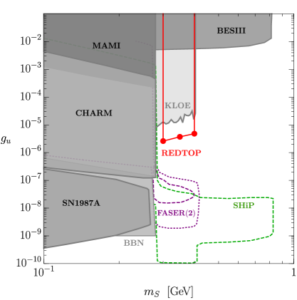
Figure 4: REDTOP sensitivity to the the hadrophilic scalar model, Eq. (21), in the $\eta\rightarrow\pi^{0}S$, $S\rightarrow\pi^{+}\pi^{-}$ mode. We display the projected sensitivity of REDTOP (red) in the $m_{S}-g_{u}$ plane to the bump hunt analysis presented in Section X.5 based on $3.3\times{10}^{18}$ POT for the three mass points $m_{S}={300,350,400}$ MeV. Also shown are various existing constraints and projections from other planned or proposed experiments; see Refs. (Batell et al., 2019; Kling and Trojanowski, 2021) for further details.

Two-Higgs doublet model

This model Abdallah et al. (2021) is one of the simplest possible extensions of the SM, assuming the existence of a second Higgs doublet $H$ and a dark singlet real scalar $h^{\prime}$. It was initially introduced to explain the anomalies observed by LSND, MiniBooNE and muon g−2 experiment, and it is being extended to the decays of the $\eta\rightarrow\pi^{0}h^{\prime}/H$ and $\eta^{\prime}\rightarrow\pi^{0}h^{\prime}/H$. Preliminary calculations indicate that BR($\eta\rightarrow\pi^{0}h^{\prime}$)$\sim$10^-9 while BR($\eta^{\prime}\rightarrow\pi^{0}H$)$\sim$10^-10, in both cases within REDTOP sensitivity.

A scalar $H$ could be observed in an $\eta/\eta^{\prime}$ final state in association with a $\pi^{0}$ by detecting the following processes:

$$\eta\rightarrow\pi^{0}H\rightarrow\pi^{0}+l^{+}l^{-},$$ (23)

$$\eta\rightarrow\pi^{0}H\rightarrow\pi^{0}+\pi^{+}\pi^{-}.$$ (24)

Within the SM, process (23) can only occur via a two-photon exchange diagram with a branching ratio of the order of $10^{-9}$. If such a light particle exists, even with a mass larger than the $\eta/\eta^{\prime}$ meson, which couples the leptons to the quarks, the probability for this process could be increased by several orders of magnitude, changing dramatically the dynamics of the process. Two groups of theoretical models postulating a BSM light scalar are receiving great attention lately: the Minimal Extension of the Standard Model Scalar Sector (O’Connell et al., 2007a; Krnjaic, 2016) and the models containing Higgs bosons with large couplings to light quarks (Batell et al., 2019; Egana-Ugrinovic et al., 2019b). From the experimental point of view, these models are complementary: the former predicting large coupling to the $b$-quark and to gluons but a small one to the light quarks, while the latter predicts a large coupling to light quarks. An observation at an $\eta/\eta^{\prime}$ factory of the process (23) would be an indication that the second set of models would be the most likely extension to the SM. Vice-versa, an observation of a scalar at a $B$-factory but not at REDTOP would favor the first group of models.

A detailed simulation of the process (23) and of the foreseen background, including many instrumental effects, has been performed by the Collaboration within the “Physics Beyond Collider” program (Alemany et al., 2019) assuming the Minimal Extension of the Standard Model Scalar model.

An integrated beam flux of $10^{12}$ POT (as available at CERN, see Sec. XVII below) has been assumed. A simple “bump-hunt” analysis was performed, looking at the invariant mass of di-leptons associated to a prompt photon. The sensitivity to the $\sin^{2}\theta$ parameter (O’Connell et al., 2007a; Krnjaic, 2016) is shown in Fig. 4. The largest contributing background was found to be from the 3-body decay $\eta\rightarrow\gamma+l^{+}l^{-}$ where an extra $\gamma$ fakes a $\pi^{0}$ in the final state.

A preliminary sensitivity analysis for several experiments (including REDTOP) based on the second set of models can be found in Ref. (Batell et al., 2019)

LSND and MiniBooNE (MB) observed an excess of electron-like events over the expected background. These excesses can be understood in the context of the decay of a heavy neutral lepton ($N_{2}$) produced via up-scattering of the beam $\nu_{\mu}$ in the detector Abdallah et al. (2021). Once $N_{2}$ is produced, it decays instantaneously to another neutral lepton ($N_{1}$) and a light scalar ($h^{\prime}$). The $h^{\prime}$ subsequently decays promptly to a collimated $e^{+}e^{-}$ pair producing a signal in the detectors. The solution is set in the context of a two-Higgs doublet model (2HDM) $(\phi_{h},\phi_{H})$ and a dark singlet real scalar $\phi_{h^{\prime}}$. After diagonalization of the mass matrix, one SM-like higgs ($h$) and two other light scalars ($h^{\prime},H$) have been obtained. In this model, only the $\phi_{h}$ acquires a vacuum expectation value (VEV). Hence, the coupling of $\phi_{H}$ with fermions is an independent parameter. The model has three right-handed neutrinos $N_{i}$ ($i=1,2,3$) which are responsible for producing light neutrino masses via a type-I seesaw. Two of the heavy neutral leptons participate in the production of excess events in LSND and MB, as mentioned above. The model also resolves the discrepancy between theory and experiment in the anomalous magnetic moment of muon via the contributions of the light scalars ($h^{\prime},H$). Details of the model are given in Abdallah et al. (2021). The benchmark point (BP) of the parameters is shown in Table 1.

$m_{N_{1}}$	$m_{N_{2}}$	$m_{N_{3}}$	$y_{u}^{h^{\prime}(H)}\!\!\times\!\!10^{6}$	$y_{e(\mu)}^{h^{\prime}}\!\!\times\!\!10^{4}$	$y_{e(\mu)}^{H}\!\!\times\!\!10^{4}$
85 MeV	$130$ MeV	$10$ GeV	$0.8(8)$	$0.23(1.6)$	$2.29(15.9)$
$m_{h^{\prime}}$	$m_{H}$	$\sin\delta$	$y_{d}^{h^{\prime}(H)}\!\!\times\!\!10^{6}$	$y_{\nu_{\!i2}}^{h^{\prime}(H)}\!\!\times\!\!10^{3}$	$\lambda_{N_{\!12}}^{h^{\prime}(H)}\!\!\times\!\!10^{3}$
17 MeV	750 MeV	$0.1$	$0.8(8)$	$1.25(12.4)$	$74.6(-7.5)$

Table 1: Benchmark point for LSND and MB events, and muon $g-2$ calculation.

The light scalars ($h^{\prime},H$) couple to $u$ and $d$ quarks. Hence these scalars could be probed via the decay channels of $\eta\,(\eta^{\prime})$ in REDTOP. The decay amplitudes of $\eta,\eta^{\prime}\to\pi^{0}S$ and $\eta^{\prime}\to\eta S$, where $S$ refers to the light scalars $h^{\prime},H$, are Gan et al. (2022):

$$\mathcal{A}(\eta^{(\prime)}\to\pi^{0}S) =-B_{0}\left[(\lambda_{u}-\lambda_{d})\Gamma^{u-d}_{\pi\eta^{(\prime)}}(m_{S}^{2})+(\lambda_{u}+\lambda_{d})\Gamma^{u+d}_{\pi\eta^{(\prime)}}(m_{S}^{2})+\lambda_{s}\Gamma^{s}_{\pi\eta^{(\prime)}}(m_{S}^{2})\right],$$ (25)

$$\mathcal{A}(\eta^{\prime}\to\eta S) =-B_{0}\left\{(\lambda_{u}+\lambda_{d})\Gamma^{u+d}_{\eta\eta^{(\prime)}}(m_{S}^{2})+\lambda_{s}\Gamma^{s}_{\eta\eta^{(\prime)}}(m_{S}^{2})\right\}.$$ (26)

The values of $B_{0}$ and other form factor are given in Gan et al. (2022). In this model $S$ couples exclusively to both $u$ and $d$ quarks, therefore the partial widths of $\eta,\eta^{\prime}\to\pi^{0}S$ and $\eta^{\prime}\to\eta S$ are Gan et al. (2022) given by:

$$\Gamma\big{(}\eta^{(\prime)}\to\pi^{0}S\big{)} =\frac{|\mathcal{A}(\eta^{(\prime)}\to\pi^{0}S)|^{2}}{16\pi m_{\eta^{(\prime)}}}\lambda^{1/2}\left(1,\frac{m_{\pi^{0}}^{2}}{m_{\eta^{(\prime)}}^{2}},\frac{m_{S}^{2}}{m_{\eta^{(\prime)}}^{2}}\right)\,,$$ (27)

$$\Gamma\big{(}\eta^{\prime}\to\eta S\big{)} =\frac{|\mathcal{A}(\eta^{\prime}\to\eta S)|^{2}}{16\pi m_{\eta^{(\prime)}}}\lambda^{1/2}\left(1,\frac{m_{\pi^{0}}^{2}}{m_{\eta^{(\prime)}}^{2}},\frac{m_{S}^{2}}{m_{\eta^{(\prime)}}^{2}}\right)\,,$$ (28)

where $\lambda(a,b,c)=a^{2}+b^{2}+c^{2}-2(ab+ac+bc)$.

For the benchmark parameter values, as shown in Table 1, where $\lambda^{h^{\prime}(H)}_{q}=y_{q}^{h^{\prime}(H)},\leavevmode\nobreak\ q=u,d$, and $\lambda^{h^{\prime}(H)}_{s}=0$, the partial decay widths and the branching ratios of the decay modes of $\eta$ and $\eta^{\prime}$ are presented in Tables 2, 3.

	$\Gamma(\eta\to\pi^{0}S)$ [GeV]	${\rm BR}(\eta\to\pi^{0}S)$	$\Gamma(\eta^{\prime}\to\pi^{0}S)$ [GeV]	${\rm BR}(\eta^{\prime}\to\pi^{0}S)$
$S=h^{\prime}$	$1.59\times 10^{-17}$	$1.22\times 10^{-11}$	$1.91\times 10^{-17}$	$1.01\times 10^{-13}$
$S=H$	$0$	$0$	$5.70\times 10^{-16}$	$3.03\times 10^{-12}$

Table 2: The partial decay widths and the branching ratios of the decay modes $\eta^{(\prime)}\to\pi^{0}S$, where $S=h^{\prime},H$.

	$\Gamma(\eta^{\prime}\to\eta S)$ [GeV]	${\rm BR}(\eta^{\prime}\to\eta S)$
$S=h^{\prime}$	$4.54\times 10^{-14}$	$2.41\times 10^{-10}$
$S=H$	$0$	$0$

Table 3: The partial decay width and the branching ratio of the decay mode $\eta^{\prime}\to\eta S$.

The $\pi^{0}S$ production is proportional to $(\lambda_{u}-\lambda_{d})^{2}$ which equals to zero for this BP, due to $\lambda^{h^{\prime}(H)}_{u}=\lambda^{h^{\prime}(H)}_{d}$. This assumption of equal couplings to $u$ and $d$ quarks was made for simplicity. However, we now consider a case different from the BP in Table 1 which assumes unequal couplings, bringing the dominant isovector term into play, but still keeps the LSND and MB fits intact and also leaves the muon $g-2$ calculation unaltered. We assume $\lambda^{h^{\prime}(H)}_{u}\times 10^{6}=0.86(8.6)$ and $\lambda^{h^{\prime}(H)}_{d}\times 10^{6}=0.74(7.4)$, i.e., $(\lambda^{h^{\prime}(H)}_{u}-\lambda^{h^{\prime}(H)}_{d})\times 10^{6}=0.12(1.2)$ and $\lambda^{h^{\prime}(H)}_{s}=0$. For this case, we have calculated the branching ratios of the decay modes of $\eta^{(\prime)}\to\pi^{0}S$ which are shown in Table 4. In Fig. 5, we show the branching ratios of the decay modes $\eta^{(\prime)}\to\pi^{0}S$ as a function of $(\lambda_{u}-\lambda_{d})^{2}$.

	${\rm BR}(\eta\to\pi^{0}S)$	${\rm BR}(\eta^{\prime}\to\pi^{0}S)$
$S=h^{\prime}$	$1.18\times 10^{-9}$	$4.17\times 10^{-12}$
$S=H$	$0$	$1.25\times 10^{-10}$

Table 4: The branching ratios of the decay modes $\eta^{(\prime)}\to\pi^{0}S$, where $S=h^{\prime},H$.

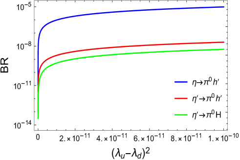
Figure 5: The branching ratios of the decay modes $\eta^{(\prime)}\to\pi^{0}S$ as a function of $(\lambda_{u}-\lambda_{d})^{2}$.

III.1.3 Heavy neutral lepton portal models

This portal operates with one or several dark heavy neutral leptons (HNLs). Among the several models existing under this portal, the Two-Higgs doublet model is the only one considered, at present, by REDTOP. The process, in this case, would be: $\eta/\eta^{\prime}\rightarrow\pi^{0}H$ with $H\rightarrow\nu N_{2}$ and $N_{2}\rightarrow h^{\prime}N_{1}$ followed by $h^{\prime}\rightarrow e^{+}e^{-}$. The process is identified by the presence of a $\pi^{0}$ and an $e^{+}e^{-}$ pair in the final state and a peak in the missing mass of the $\eta/\eta^{\prime}$ spectrum.

Two-Higgs doublet model

The 2HDM discussed in Sec. III.1.2 introduces, besides the $H$ and $h^{\prime}$ scalars, also two heavy neutral leptons, $N_{1}$ and $N_{2}$ which represent invisible components of the HNL portal. This portal could be explored by studying the process $p+Li\rightarrow\eta+X\;$with$\;\eta\rightarrow\pi^{0}H\;;\;H\rightarrow\nu N_{2}\;;\;N_{2}\rightarrow N_{1}h^{\prime}\;;\;h^{\prime}\rightarrow e^{+}e^{-},$ which is, however, particularly challenging at REDTOP, because the decay chains contains two undetected particles: $N_{1}$ and $N_{2}$. The following points may be relevant when considering detectability of the (visible) scalars in REDTOP:

• In this model Abdallah et al. (2021), the branching ratios of the decay modes of $H$, $h^{\prime}$, and $N_{2}$ for the BP in Table 1 are as follows:

  $$\!\!\!\!\!\!\!\!\!\!\!\!\!\!\!\!\!\!\!\!\!\!{\rm BR}(H\rightarrow\nu_{i}N_{2})=89.36\%,\leavevmode\nobreak\ {\rm BR}(H\rightarrow N_{1}N_{2})=10.17\%,\leavevmode\nobreak\ {\rm BR}(H\rightarrow\mu^{+}\mu^{-})=0.46\%,$$ (29)

  $$\!\!\!\!\!\!\!\!\!\!\!\!\!\!\!\!\!\!\!\!\!\!{\rm BR}(H\rightarrow e^{+}e^{-})=0.011\%,\leavevmode\nobreak\ \leavevmode\nobreak\ \!{\rm BR}(H\rightarrow\gamma\gamma)=3.54\times 10^{-6}\%,$$ (30)

  $$\!\!\!\!\!\!\!\!\!\!\!\!\!\!\!\!\!\!\!\!\!\!{\rm BR}(h^{\prime}\rightarrow e^{+}e^{-})=99.9998\%,\leavevmode\nobreak\ \leavevmode\nobreak\ \leavevmode\nobreak\ \leavevmode\nobreak\ \leavevmode\nobreak\ {\rm BR}(h^{\prime}\rightarrow\gamma\gamma)=2\times 10^{-4}\%,$$ (31)

  $$\!\!\!\!\!\!\!\!\!\!\!\!\!\!\!\!\!\!\!\!\!\!{\rm BR}(N_{2}\rightarrow N_{1}h^{\prime})=99.94\%,\leavevmode\nobreak\ \leavevmode\nobreak\ {\rm BR}(N_{2}\rightarrow\nu_{i}h^{\prime})=0.06\%.\leavevmode\nobreak\ \leavevmode\nobreak\$$ (32)

• It is assumed that $N_{1}$ could decay to invisible particles and also there is a possibility to tune the parameters such that $N_{1}$ becomes a long-lived particle.

• Thus, an $H$, when produced in the detector, decays with $89.36\%$ BR to $N_{2}$ and an active SM neutrino. The former, in turn will promptly decay to an $N_{1}$ and $h^{\prime}$, leading to a visible $e^{+}e^{-}$ pair with missing energy.

• For the BP in Table 1, the total decay width of $H$, $h^{\prime}$ and $N_{2}$ are $1.45\times 10^{-5}$ GeV, $3.56\times 10^{-13}$ GeV, and $2.07\times 10^{-5}$ GeV, respectively. Hence all the particles will decay inside the REDTOP.

III.1.4 The visible QCD axion

The original incarnation of the QCD axion (the so-called ‘PQWW’ axion Peccei and Quinn (1977b, c); Weinberg (1978b); Wilczek (1978)) was a simple Two-Higgs-Doublet Model (2HDM) with a common breaking mechanism for the Electroweak and PQ symmetries. By the late 80s, the parameter space of the PQWW axion was fully excluded by searches for axionic production in hadronic decays and beam dump experiments. Still, many variants of the original QCD axion have been explored (see, e.g., Bardeen et al. (1987)), and more recently, Alves and Weiner have shown that a variant of the QCD axion with $m_{a}\sim\mathcal{O}(1-10)$ MeV and $f_{a}\sim\mathcal{O}(1-10)$ GeV remains viable Alves and Weiner (2018).

In this variant, the PQ mechanism is implemented by new dynamics at the GeV scale coupling predominantly to the first generation of Standard Model fermions. The resulting QCD axion is short-lived and decays to $e^{+}e^{-}$ with a lifetime $\tau_{a}\lesssim 10^{-13}$ s Andreev et al. (2021), avoiding constraints from beam dumps and fixed target experiments, as well as from upper bounds on rare meson/quarkonium decays to a long-lived axion that escapes detection. Furthermore, this axion couples to the first generation of SM quarks with a special relation between the ratios of light quark masses and their PQ charges, namely,

$$\frac{m_{u}}{m_{d}}\leavevmode\nobreak\ \simeq\leavevmode\nobreak\ \frac{Q^{{}_{\text{PQ}}}_{d}}{Q^{{}_{\text{PQ}}}_{u}}\leavevmode\nobreak\ =\leavevmode\nobreak\ \frac{1}{2}\;.$$

This relation causes an accidental cancellation of the leading order $\chi$PT contribution to axion-pion mixing,

$$\theta_{a\pi}\leavevmode\nobreak\ \leavevmode\nobreak\ =\leavevmode\nobreak\ \leavevmode\nobreak\ -\leavevmode\nobreak\ \frac{f_{\pi}}{f_{a}}\,\left[\frac{(m_{u}\,Q^{{}_{\text{PQ}}}_{u}-m_{d}\,Q^{{}_{\text{PQ}}}_{d})}{m_{u}+m_{d}}\leavevmode\nobreak\ +\leavevmode\nobreak\ \mathcal{O}\left(\frac{m_{ud}}{m_{s}}\right)\right]\leavevmode\nobreak\ \leavevmode\nobreak\ \simeq\leavevmode\nobreak\ \leavevmode\nobreak\ \frac{\leavevmode\nobreak\ (-0.2\pm 30)\times 10^{-4}\leavevmode\nobreak\ }{(f_{a}/\text{GeV)}}\,,$$ (33)

which results in a QCD axion with suppressed isovector couplings. This piophobic axion is therefore safe from bounds from $\pi^{+}\rightarrow a\,e^{+}\nu_{e}$ mediated via $a-\pi^{0}$ mixing. In addition, bounds from $K^{+}\rightarrow\pi^{+}a$, previously believed to be severe, were shown to suffer from large hadronic uncertainties that preclude the exclusion of significant portions of the piophobic axion parameter space.

There are several motivations for searching for such an axion Alves (2021):

• First and foremost, the QCD axion is tied to the solution of the strong CP problem, which is one of the most significant puzzles in theoretical physics.

• In addition, a piophobic QCD axion with mass of $\sim 16-17$ MeV could explain the recent anomalies in isoscalar magnetic transitions of ${}^{8}\text{Be}$ and ${}^{4}\text{He}$ nuclei Krasznahorkay et al. (2016, 2019), while simultaneously explaining the absence of anomalous emissions in isovector and/or electric radiative nuclear processes Zhang and Miller (2021).

• Finally, the suppressed axion-pion mixing in (33) could explain the anomalous rate for $\pi^{0}\to e^{+}e^{-}$ measured by the KTeV collaboration Abouzaid et al. (2007).

Because the QCD axion couples to quarks and/or gluons, it should invariably lead to new signals in $\eta^{(\prime)}$ decays. The simplest such signal is a contribution to $\eta^{(\prime)}\to e^{+}e^{-}$ due to $a-\eta^{(\prime)}$ mixing. Since the SM expectation for $\text{Br}\big{(}\eta^{(\prime)}\to e^{+}e^{-}\big{)}$ is still two orders of magnitude below current experimental sensitivity, there is significant room for new physics contributions to this final state. REDTOP should have an expected sensitivity to $\text{Br}\big{(}\eta\to e^{+}e^{-}\big{)}$ with $\mathcal{O}(10^{-10})$ precision, and to $\text{Br}\big{(}\eta^{\prime}\to e^{+}e^{-}\big{)}$ with $\mathcal{O}(10^{-9})$ precision, which should lead to a sensitivity to $a-\eta^{(\prime)}$ mixing angles of order $\theta_{a\eta}\sim\mathcal{O}(10^{-4})$ and $\theta_{a\eta^{\prime}}\sim\mathcal{O}(10^{-2})$, respectively (see Alves (2021), Sec. VIII, and Table 34).

Firmer evidence for the QCD axion, however, would come as an observation of axio-hadronic $\eta^{(\prime)}\to\pi\pi a$ decays. In fact, a new pseudoscalar particle appearing in $\eta^{(\prime)}$ decays would only be possible if it coupled to quarks and/or gluons. As such, it would affect the QCD topological vacuum by either (i) contributing to or (ii) canceling the strong CP phase $\theta_{\text{QCD}}$. In case (i), such pseudoscalar would be characterized as a generic ‘axion-like particle’ (ALP), albeit this would be an extremely ad hoc and fine-tuned scenario since another BSM mechanism would then have to be concocted to cancel the ALP’s contribution to $\theta_{\text{QCD}}$. Therefore, option (ii) would be a more compelling interpretation for such an observation, namely, that a new light pseudoscalar $a$ appearing in $\eta^{(\prime)}\to\pi\pi a$ must be the QCD axion which dynamically relaxes $\theta_{\text{QCD}}$ to zero and solves the strong CP problem.

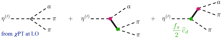
Figure 6: Contributions to the amplitude $\mathcal{A}(\eta^{(\prime)}\to\pi\pi a)$ in the framework of Resonance Chiral Theory. Left graph: leading order quartic term. Middle and right graphs: exchange of low-lying scalar resonances. The dimensionless couplings $\widehat{c}_{d}$ and $\widehat{c}_{m}$ are expected to deviate from the large-$N_{c}$ limit of $|\widehat{c}_{d}|=|\widehat{c}_{m}|=1$ by $\mathcal{O}(10\%)$.

Low-energy strong interaction effects, however, introduce large uncertainties to the calculation of axio-hadronic $\eta$ and $\eta^{\prime}$ decays. In Alves (2021), this calculation was performed in the framework of Resonance Chiral Theory (R$\chi$T), an interpolating effective theory between the low-energy $\chi$PT framework and the microscopic QCD description. R$\chi$T encodes the most prominent features of nonperturbative strong dynamics by incorporating the low-lying QCD resonances and extending the principle of vector meson dominance Ecker et al. (1989). In this framework, exchanges of $0^{++}$ resonances such as the $a_{0}(980)$ and $f_{0}(980)$ contribute to the amplitude for $\eta^{(\prime)}\to\pi\pi a$, see Fig. 6. These contributions are of the same order of magnitude as the $\chi$PT quartic coupling contribution, and significant destructive interference between these amplitudes can take place within the expected range of couplings between $a_{0}(980)$, $f_{0}(980)$ and $\pi$, $a$, $\eta^{(\prime)}$. The resulting branching ratios for axio-hadronic $\eta^{(\prime)}$ decays can vary significantly depending on the degree of destructive interference between amplitudes. For the case of the piophobic QCD axion explaining the ${}^{8}\text{Be}$ and ${}^{4}\text{He}$ anomalies, the branching ratios for $\eta^{(\prime)}\to\pi\pi a$ are shown in Fig. 7 as a function $\widehat{c}_{d}$ and $\widehat{c}_{m}$, which parametrize the couplings between the octet scalars and the chiral mesons. Previous $\eta^{(\prime)}$-decay searches in $\pi\pi e^{+}e^{-}$ final states have not been able to probe this scenario. In fact, an excess of 27 events (vs 7.7 expected) in that mass region was observed by CELSIUS/WASA in the $\eta\rightarrow\pi^{+}\pi^{-}e^{+}e^{-}$ process Bargholtz et al. (2007). A similar excess was also observed by BESIII in the $\eta^{\prime}\rightarrow\pi^{+}\pi^{-}e^{+}e^{-}$ process Ablikim et al. (2013), although it was dismissed as background from $\gamma$-conversion. Despite the two-orders-of-magnitude variation in these branching ratios, they are fully within the expected REDTOP sensitivity to $\eta^{(\prime)}\to\pi\pi(a\to e^{+}e^{-})$ final states. Therefore, REDTOP will definitively probe the remaining parameter space of the visible QCD axion.

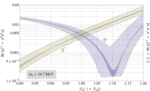
Figure 7: Estimated branching ratios for $\eta^{(\prime)}\to\pi\,\pi\,a$ as a function of the scalar octet couplings to the light pseudoscalar mesons (taken from Alves (2021)). The width of the blue and brown bands result from varying the masses and widths of the scalar resonances, $a_{0}$ and $f_{0}$, within their experimental uncertainties. For the narrow bands with darker shading, the scalar masses were fixed to $m_{a_{0}}=m_{f_{0}}=980\,$MeV, and their widths were varied within the ranges $\Gamma_{a_{0}}=(40-100)\,$MeV, $\Gamma_{f_{0}}=(10-200)\,$MeV. The broader, lighter shaded bands resulted from additionally varying the scalar masses within the ranges $m_{a_{0}},\,m_{f_{0}}=(960-1000)\,$MeV.

III.1.5 Axion-like particles

More generally, axio-hadronic decays of the $\eta$ and $\eta^{\prime}$ can also probe axion-like particles (ALPs), which have the same types of interactions as the QCD axion but receive an additional, PQ-breaking contribution to their masses. As such, ALP models have a broader parameter space than the QCD axion since the ALP mass and decay constant are independent parameters.

The ALP interactions that contribute most significantly to axio-hadronic $\eta^{(\prime)}$ decays are:

$$\mathcal{L}_{\text{ALP}}^{(Y)}\leavevmode\nobreak\ \supset\leavevmode\nobreak\ -c_{GG}\,\frac{\alpha_{s}}{4\pi}\,\frac{a}{f_{a}}G\widetilde{G}\leavevmode\nobreak\ +\leavevmode\nobreak\ \sum_{q=u,d,s}\leavevmode\nobreak\ m_{q}\,\leavevmode\nobreak\ \bar{q}\,e^{i\,c_{q}\frac{a}{f_{a}}\gamma_{5}}q\leavevmode\nobreak\ -\leavevmode\nobreak\ M_{\;{/\!\!\!\!\!\text{\tiny PQ}}}^{2}\,\frac{a^{2}}{2}\,,$$ (34)

where $a$ denotes an ALP with decay constant $f_{a}$, $M_{\;{/\!\!\!\!\!\text{\tiny PQ}}}$ is a PQ-breaking contribution to the ALP mass, and the quarks $q=u,d,s$ are written in the mass eigenstate basis. Furthermore, (34) is defined at the GeV scale, the heavy-flavor quarks $c,b,t$ having been integrated out. If they carry PQ charges $c_{c}$, $c_{b}$, and $c_{t}$, respectively, then they will implicitly contribute to the gluonic ALP coupling through

$$c_{GG}\leavevmode\nobreak\ =\leavevmode\nobreak\ c_{GG}^{\text{\tiny UV}}\leavevmode\nobreak\ +\leavevmode\nobreak\ \sum_{\;q=c,b,t}\,\frac{c_{q}}{2}\,.$$ (35)

By performing ALP-dependent quark chiral rotations, the ALP interactions in (34) can be recast in another commonly considered basis in the recent literature:

$$\mathcal{L}_{\text{ALP}}^{(\partial)}\leavevmode\nobreak\ \supset\leavevmode\nobreak\ -\left(c_{GG}+\sum_{q}\,\frac{c_{q}}{2}\right)\frac{\alpha_{s}}{4\pi}\,\frac{a}{f_{a}}G\widetilde{G}\leavevmode\nobreak\ +\leavevmode\nobreak\ \frac{\partial_{\mu}a}{f_{a}}\leavevmode\nobreak\ \sum_{q}\,\frac{c_{q}}{2}\;\bar{q}\,\gamma^{\mu}\gamma_{5}\,q\leavevmode\nobreak\ -\leavevmode\nobreak\ M_{\;{/\!\!\!\!\!\text{\tiny PQ}}}^{2}\,\frac{a^{2}}{2}$$ (36a)

$$\leavevmode\nobreak\ \leavevmode\nobreak\ +\leavevmode\nobreak\ \sum_{i,j}\leavevmode\nobreak\ \frac{g_{2}}{\sqrt{2}\,}\;V^{\text{\tiny CKM}}_{ij}\leavevmode\nobreak\ W_{\mu}^{+}\leavevmode\nobreak\ \leavevmode\nobreak\ \bar{u}_{L}^{i}\,e^{-i\Big{(}\!\frac{\,c_{u_{i}}-c_{d_{j}}\,}{2}\frac{a}{f_{a}}\gamma_{5}\!\Big{)}}\gamma^{\mu}\,d_{L}^{j}\leavevmode\nobreak\ +\leavevmode\nobreak\ \text{h.c.}$$ (36b)

Note that the “Yukawa basis” in (34) and the “derivative basis” in (36a) are equivalent as long as the weak interactions are neglected. (The failure to account for the additional terms in (36b) has led to much confusion in the literature and convoluted treatments of axio-hadronic Kaon decays, e.g., Bauer et al. (2021).)

However, because axio-hadronic $\eta^{(\prime)}$ decays do not violate flavor, this basis equivalency issue between (34) and (36a) is irrelevant for the decays we will consider in this subsection. For the same reason, more generic derivative ALP couplings to axial and vector flavor-changing neutral currents are also irrelevant. Therefore, for the remainder of this subsection we will adopt the simpler, “Yukawa basis” parametrization of the ALP couplings in (34).

In order to extract the amplitude for $\eta^{(\prime)}\to\pi\pi a$ from (34), three basic steps are needed:

1. The QCD level ALP-interactions in (34) must be mapped into chiral perturbation theory ($\chi$PT), i.e., they must be re-expressed in terms of ALP couplings to mesonic degrees of freedom.

2. The mass matrix and kinetic mixing terms must be diagonalized in order to obtain the physical ALP state $a_{\text{\tiny phys}}$ and the low energy meson states $\pi^{0}$, $\eta$, and $\eta^{\prime}$.

3. The $\chi$PT Lagrangian must be re-expressed in terms of the physical states, so that the quartic interactions $\eta^{(\prime)}$-$\pi$-$\pi$-$a_{\text{\tiny phys}}$ can be obtained.

A proper treatment and execution of steps 1$-$3 outlined above is still missing in the ALP literature. Firstly, to properly describe the octet-singlet composition of the $\eta$ and the $\eta^{\prime}$, as well as their mixing with the ALP, one needs to go beyond leading order in $\chi$PT. Secondly, (axio)-hadronic $\eta^{(\prime)}$ decays receive significant nonperturbative corrections which require going beyond $\chi$PT, such as, e.g., accounting for strong final state rescattering via dispersive relations, or including the exchange of the low energy QCD resonances via Resonance Chiral Theory. Here, we will not address either of these issues (work in preparation in these directions will appear in Alves and Gonzàlez-Solís (2022)). We will simply follow recent naïve, leading order $\chi$PT treatments to obtain the amplitude for axio-hadronic $\eta^{(\prime)}$ decays. As such, our results should be considered a rough, order-of-magnitude estimate of the rate for $\eta^{(\prime)}\to\pi\pi a$ to qualitatively assess REDTOP’s sensitivity reach to the parameter space of hadronic ALPs.

The implementation of step 1 above at leading order in $\chi$PT amounts to mapping (34) into:

$$\mathcal{L}_{\text{ALP}}^{(\chi\text{PT}\text{@LO})}\,=\leavevmode\nobreak\ -\frac{M_{0}^{2}}{2}\left(\eta_{0}-\frac{c_{GG}}{\sqrt{3/2}\,}\frac{f_{\pi}}{f_{a}}\,a\right)^{2}\,+\;\frac{f_{\pi}^{2}}{4}\,\text{Tr}\big{[}2B_{0}M_{q}(a)U\,+\,\text{h.c.}\big{]}\,-\,M_{\;{/\!\!\!\!\!\text{\tiny PQ}}}^{2}\frac{a^{2}}{2}\,,$$ (37)

where $M_{0}\sim\mathcal{O}$(GeV) parametrizes the large strong anomaly contribution to the mass of the $\eta^{\prime}$, $B_{0}=-\langle q\bar{q}\rangle/f_{\pi}^{2}$, $M_{q}(a)$ is the ALP-dependent quark mass matrix,

$$M_{q}(a)\equiv\begin{pmatrix}\,m_{u}\,e^{i\,c_{u}a/f_{a}}\!\!\!&&\\ &\!\!\!m_{d}\,e^{i\,c_{d}\,a/f_{a}}\!\!\!&\\ &&\!\!\!m_{s}\,\,e^{i\,c_{s}\,a/f_{a}}\end{pmatrix},$$ (38)

and $U$ denotes the non-linear representation of the chiral meson nonet,

$$U\leavevmode\nobreak\ =\leavevmode\nobreak\ \text{Exp}\frac{i}{f_{\pi}}\,\begin{pmatrix}\vspace{0.17cm}\pi^{0}+\frac{\eta_{8}}{\sqrt{3}}+\frac{\eta_{0}}{\sqrt{3/2}}&\sqrt{2}\,\pi^{+}&\sqrt{2}\,K^{+}\\ \vspace{0.17cm}\sqrt{2}\,\pi^{-}&-\pi^{0}+\frac{\eta_{8}}{\sqrt{3}}+\frac{\eta_{0}}{\sqrt{3/2}}&\sqrt{2}\,K^{0}\\ \sqrt{2}\,K^{-}&\sqrt{2}\,\overline{K}^{0}&-\frac{2\,\eta_{8}}{\sqrt{3}}+\frac{\eta_{0}}{\sqrt{3/2}}\leavevmode\nobreak\ \end{pmatrix}.$$ (39)

Even though we are restricting our calculation to the naïve leading order $\chi$PT treatment, we will introduce a small improvement by adopting the two-mixing-angle scheme to express the physical $\eta$ and $\eta^{\prime}$ states in the octet-singlet basis as

$$\eta_{0}\leavevmode\nobreak\ = \leavevmode\nobreak\ \;\frac{f_{\pi}}{f_{0}}\,\big{(}\!\cos\theta_{0}\,\eta^{\prime}\,-\,\sin\theta_{0}\,\eta\big{)}\,,$$ (40a)

$$\eta_{8}\leavevmode\nobreak\ = \leavevmode\nobreak\ \;\frac{f_{\pi}}{f_{8}}\,\big{(}\!\sin\theta_{8}\,\eta^{\prime}\,+\,\cos\theta_{8}\,\eta\big{)}\,.$$ (40b)

For concreteness, we will take the values $\theta_{8}=-24^{\circ}$, $\theta_{0}=-2.5^{\circ}$, $f_{8}=1.51\,f_{\pi}$, and $f_{0}=1.29\,f_{\pi}$ from the unconstrained fit in Escribano and Frere (2005).

Step 2 is the non-trivial part of our calculation, and will involve obtaining the ALP mixing angles $\theta_{a\pi}$, $\theta_{a\eta_{8}}$, $\theta_{a\eta_{0}}$ with $\pi^{0}$, $\eta_{8}$, $\eta_{0}$, respectively. Because of our judicious choice of ALP basis with no kinetic mixing terms, our work is greatly simplified: the ALP-meson mixing angles can be simply obtained by diagonalizing the ALP-meson mass matrix in (37). While this can be done straightforwardly numerically, a parametric dependence of the mixing angles on $m_{a}$, $f_{a}$, $c_{q}$ and $c_{GG}$ is desirable. This can be obtained by considering the following.

First, in the PQ preserving limit of $M_{\;{/\!\!\!\!\!\text{\tiny PQ}}}=0$ and $m_{a}\ll m_{\pi}$ (i.e., when $a$ is the QCD axion), we have

$$(m_{a}^{\text{\tiny(PQ)}})^{2}\leavevmode\nobreak\ =\leavevmode\nobreak\ \frac{(c_{u}+c_{d}+c_{s}+2\,c_{GG})^{2}}{(1+\epsilon_{\eta\eta^{\prime}})}\,\frac{m_{u}m_{d}}{(m_{u}+m_{d})^{2}}\,\frac{m_{\pi}^{2}\,f_{\pi}^{2}}{f_{a}^{2}}\,,$$ (41)

and

$$\theta_{a\pi}^{{}^{\text{\tiny(PQ)}}}= -\frac{f_{\pi}}{f_{a}}\,\frac{1}{(1+\epsilon_{\eta\eta^{\prime}})}\,\bigg{(}\frac{\,(c_{u}m_{u}-c_{d}m_{d})\,+\,(c_{s}+2c_{GG})(m_{u}-m_{d})/2\,}{m_{u}+m_{d}}+\epsilon_{\eta\eta^{\prime}}\,\frac{\,(c_{u}-c_{d})\,}{2}\bigg{)}$$ (42a)

$$\theta_{a\eta_{8}}^{{}^{\text{\tiny(PQ)}}}= \leavevmode\nobreak\ \leavevmode\nobreak\ \frac{f_{\pi}}{f_{a}}\,\frac{\sqrt{3}}{\leavevmode\nobreak\ 2}\;\frac{1}{(1+\epsilon_{\eta\eta^{\prime}})}\;\bigg{(}c_{s}+\frac{2}{3}\,c_{GG}-\epsilon_{\eta\eta^{\prime}}\frac{\,(c_{u}+c_{d}+4c_{GG}/3)+(c_{u}+c_{d}-2c_{s})\,2m_{\!K}^{2}/m_{\!\eta^{\prime}}^{2}\,}{1+6m_{\!K}^{2}/m_{\!\eta^{\prime}}^{2}}\bigg{)}$$ (42b)

$$\theta_{a\eta_{0}}^{{}^{\text{\tiny(PQ)}}}= \leavevmode\nobreak\ \leavevmode\nobreak\ \frac{f_{\pi}}{f_{a}}\;\bigg{(}\frac{c_{GG}}{\sqrt{3/2}\,}\,-\,\frac{m_{\pi}^{2}}{m_{\eta^{\prime}}^{2}}\,\frac{\sqrt{6}\,(c_{u}+c_{d}+c_{s}+2c_{GG})}{1+\epsilon_{\eta\eta^{\prime}}}\frac{m_{u}m_{d}}{(m_{u}+m_{d})^{2}}\bigg{)}$$ (42c)

where

$$\epsilon_{\eta\eta^{\prime}}\leavevmode\nobreak\ \equiv\leavevmode\nobreak\ \frac{m_{u}m_{d}}{m_{s}(m_{u}+m_{d})}\;\bigg{(}1+6\,\frac{m_{K}^{2}}{m_{\eta^{\prime}}^{2}}\bigg{)}\leavevmode\nobreak\ \simeq\leavevmode\nobreak\ 0.04\,.$$ (43)

This can be generalized to the PQ-breaking case of a generic ALP as

$$m_{a}^{2}\leavevmode\nobreak\ =\leavevmode\nobreak\ (m_{a}^{\text{\tiny(PQ)}})^{2}\,+\,M_{\;{/\!\!\!\!\!\text{\tiny PQ}}}^{2}\,,$$ (44)

and

$$\theta_{a\pi}=\theta_{a\pi}^{{}^{\text{\tiny(PQ)}}}\bigg{(}1\,+\,\frac{m_{a}^{2}}{m_{\pi}^{2}-m_{a}^{2}}\bigg{)}$$ (45a)

$$\theta_{a\eta_{8}}=\frac{1}{f_{8}}\,\bigg{[}\!\cos{\theta_{8}}\bigg{(}\frac{f_{8}\cos{\theta_{0}}\,\theta_{a\eta_{8}}^{{}^{\text{\tiny(PQ)}}}-f_{0}\sin{\theta_{8}}\,\theta_{a\eta_{0}}^{{}^{\text{\tiny(PQ)}}}}{\cos{(\theta_{8}-\theta_{0})}}\bigg{)}\bigg{(}1\,+\,\frac{m_{a}^{2}}{\,m_{\eta}^{2}-m_{a}^{2}\,}\bigg{)}\,+$$

$$\qquad\qquad\quad\sin{\theta_{8}}\bigg{(}\frac{f_{0}\cos{\theta_{8}}\,\theta_{a\eta_{0}}^{{}^{\text{\tiny(PQ)}}}+f_{8}\sin{\theta_{0}}\,\theta_{a\eta_{8}}^{{}^{\text{\tiny(PQ)}}}}{\cos{(\theta_{8}-\theta_{0})}}\bigg{)}\bigg{(}1\,+\,\frac{m_{a}^{2}}{\,m_{\eta\prime}^{2}-m_{a}^{2}\,}\bigg{)}\bigg{]}$$ (45b)

$$\theta_{a\eta_{0}}=\frac{1}{f_{0}}\,\bigg{[}\!-\sin{\theta_{0}}\bigg{(}\frac{f_{8}\cos{\theta_{0}}\,\theta_{a\eta_{8}}^{{}^{\text{\tiny(PQ)}}}-f_{0}\sin{\theta_{8}}\,\theta_{a\eta_{0}}^{{}^{\text{\tiny(PQ)}}}}{\cos{(\theta_{8}-\theta_{0})}}\bigg{)}\bigg{(}1\,+\,\frac{m_{a}^{2}}{\,m_{\eta}^{2}-m_{a}^{2}\,}\bigg{)}\,+$$

$$\qquad\qquad\quad\leavevmode\nobreak\ \leavevmode\nobreak\ \leavevmode\nobreak\ \cos{\theta_{0}}\bigg{(}\frac{f_{0}\cos{\theta_{8}}\,\theta_{a\eta_{0}}^{{}^{\text{\tiny(PQ)}}}+f_{8}\sin{\theta_{0}}\,\theta_{a\eta_{8}}^{{}^{\text{\tiny(PQ)}}}}{\cos{(\theta_{8}-\theta_{0})}}\bigg{)}\bigg{(}1\,+\,\frac{m_{a}^{2}}{\,m_{\eta\prime}^{2}-m_{a}^{2}\,}\bigg{)}\bigg{]}.$$ (45c)

Expression (45a) for the ALP-pion mixing angle $\theta_{a\pi}$ holds as long as $m_{a}$ is not too close to $m_{\pi^{0}}$. Similarly, (45b) and (45c) hold as long as $m_{a}$ is not too close to either $m_{\eta}$ or $m_{\eta^{\prime}}$.

We can finally proceed to step 3 by re-expressing the ALP Lagrangian in terms of the physical ALP:

$$\mathcal{L}_{\text{ALP}}^{(\chi\text{PT}\text{@LO})}\bigg{|}_{\pi^{0}\,\to\,\pi^{0}+\theta_{a\pi}a\leavevmode\nobreak\ \leavevmode\nobreak\ ,\leavevmode\nobreak\ \leavevmode\nobreak\ \eta_{8}\,\to\,\eta_{8}+\theta_{a\eta_{8}}a\leavevmode\nobreak\ \leavevmode\nobreak\ ,\leavevmode\nobreak\ \leavevmode\nobreak\ \eta_{0}\,\to\,\eta_{0}+\theta_{a\eta_{0}}a\leavevmode\nobreak\ \leavevmode\nobreak\ ,\leavevmode\nobreak\ \leavevmode\nobreak\ a\,\to\,a-\theta_{a\pi}\pi^{0}-\theta_{a\eta_{8}}\eta_{8}-\theta_{a\eta_{0}}\eta_{0}}\,,$$ (46)

from which we obtain the leading order $a$-$\pi$-$\pi$-$\eta^{(\prime)}$ quartic couplings,

$$\mathcal{L}_{\text{ALP}}^{(\chi\text{PT}\text{@LO})}\leavevmode\nobreak\ \supset\leavevmode\nobreak\ \lambda_{0}\,a\,\left(\pi^{+}\pi^{-}+\frac{\pi^{0}\pi^{0}}{2}\right)\left(\!\frac{\eta_{8}}{\sqrt{3}\,}+\frac{\eta_{0}}{\sqrt{3/2}\,}\!\right)\,,$$ (47)

where

$$\lambda_{0}\,\leavevmode\nobreak\ =\leavevmode\nobreak\ \frac{m_{\pi}^{2}}{f_{\pi}^{2}}\,\left(\frac{\,(c_{u}m_{u}+c_{d}m_{d})\,}{(m_{u}+m_{d})}\frac{f_{\pi}}{f_{a}}\,+\,\frac{\,(m_{u}-m_{d})\,}{(m_{u}+m_{d})}\,\theta_{a\pi}\,+\,\frac{\theta_{a\eta_{8}}}{\sqrt{3}\,}+\,\frac{\theta_{a\eta_{0}}}{\sqrt{3/2}\,}\right)\,.$$ (48)

We can now turn our focus specifically to $\eta\to\pi\pi a$. The amplitude for this decay then follows from (47) and (48) straightforwardly:

$$\mathcal{A}_{\eta\to\pi\pi a}\leavevmode\nobreak\ \equiv \leavevmode\nobreak\ \mathcal{A}(\eta\to\pi^{0}\pi^{0}a)\leavevmode\nobreak\ =\leavevmode\nobreak\ \mathcal{A}(\eta\to\pi^{+}\pi^{-}a)$$ (49)

$$= \leavevmode\nobreak\ \lambda_{0}\,\left(\frac{f_{\pi}}{f_{8}}\,\frac{\cos\theta_{8}}{\sqrt{3}}\,-\,\frac{f_{\pi}}{f_{0}}\,\frac{\sin\theta_{0}}{\sqrt{3/2}}\right).$$

Since the decay amplitude (49) is flat in the Dalitz phase-space, the differential rate for $\eta\to\pi\pi a$ as a function of the ALP 3-momentum $|\vec{p}_{a}|$ in the $\eta$ rest frame has a closed analytical form:

$$\frac{d\Gamma}{d|\vec{p}_{a}|}\leavevmode\nobreak\ = \leavevmode\nobreak\ \frac{1}{S_{\pi\pi}}\,\frac{|\mathcal{A}_{\eta\to\pi\pi a}|^{2}}{(4\pi)^{3}}\;\frac{|\vec{p}_{a}|^{2}}{m_{\eta}\,E_{a}}\,\sqrt{1-\frac{4\,m_{\pi}^{2}}{(p_{\eta}-p_{a})^{2}}}$$

$$= \leavevmode\nobreak\ \frac{1}{S_{\pi\pi}}\,\frac{|\mathcal{A}_{\eta\to\pi\pi a}|^{2}}{(4\pi)^{3}}\;\frac{|\vec{p}_{a}|^{2}}{m_{\eta}}\,\sqrt{\frac{m_{\eta}^{2}+m_{a}^{2}-2\,m_{\eta}\sqrt{m_{a}^{2}+|\vec{p}_{a}|^{2}}-4\,m_{\pi}^{2}}{(\,m_{\eta}^{2}+m_{a}^{2}-2\,m_{\eta}\sqrt{m_{a}^{2}+|\vec{p}_{a}|^{2}\,}\,)(\,m_{a}^{2}+|\vec{p}_{a}|^{2})}}\,,$$

where the combinatorial factor $S_{\pi\pi}$ takes the values $S_{\pi^{0}\pi^{0}}=2$ and $S_{\pi^{+}\pi^{-}\!}=1$.

To assess REDTOP’s reach in the ALP parameter space, we consider two common benchmark scenarios that have been broadly adopted in Snowmass studies of ALPs:

• Gluon dominance, which assumes that the ALP couples predominantly to heavy BSM colored fermions at UV scales above $f_{a}$. Once these fermions are integrated out, the ALP couplings expressed in terms of (34) are given by $c_{GG}^{\text{\tiny UV}}\neq 0$ and $c_{q}=0$ for all six SM quark flavors.

• Quark dominance, which assumes that the ALP couples predominantly to SM quarks, with no BSM contributions to the gluonic ALP coupling, i.e., $c_{GG}^{\text{\tiny UV}}=0$. We further restrict the parameter space of this benchmark scenario by imposing flavor blindness, i.e., we assume that all six quark flavors couple identically to the ALP, as parametrized by a universal coupling $c_{q}$ in (34) and (35).

Fig. 8 illustrates REDTOP’s futuristic reach in the ALP parameter space for the gluon dominance and quark dominance benchmark scenarios, assuming branching sensitivities of $\text{Br}[\eta\to\pi^{0}\pi^{0}a]=10^{-12}$ (green curves) and $\text{Br}[\eta\to\pi^{+}\pi^{-}a]=10^{-12}$ (orange curves). It is important to emphasize, however, that these futuristic projections assume that REDTOP would be sensitive to prompt, displaced, and invisible ALP decays alike.

For a more realistic near term sensitivity assuming the current REDTOP detector design, we can also estimate REDTOP’s reach to visibly-decaying ALPs, i.e., ALPs that decay to visible final states within the detector’s fiducial volume. We will make the simplified assumption that ALPs decaying within 100 cm of the $\eta$ decay vertex in the $\eta$ rest frame are visibly-decaying ALPs.

To proceed, further considerations are needed regarding the ALP couplings to photons and leptons in addition to its hadronic couplings defined in (34):

$$\mathcal{L}_{\text{ALP}}^{(Y)}\leavevmode\nobreak\ \leavevmode\nobreak\ \supset\leavevmode\nobreak\ \leavevmode\nobreak\ c_{\gamma\gamma}\,\frac{\alpha}{4\pi}\,\frac{a}{f_{a}}F\widetilde{F}\leavevmode\nobreak\ +\leavevmode\nobreak\ \sum_{\ell=e,\mu,\tau}\leavevmode\nobreak\ m_{\ell}\,\leavevmode\nobreak\ \bar{\ell}\,e^{i\,c_{\ell}\frac{a}{f_{a}}\gamma_{5}}\ell\,.$$ (51)

In particular, the ALP coupling to photons receives contributions from high UV scale dynamics, as well as from its mixing with the neutral pseudoscalar mesons and its couplings to heavy quarks and charged leptons,

$$c_{\gamma\gamma}\leavevmode\nobreak\ =\leavevmode\nobreak\ c_{\gamma\gamma}^{\text{\tiny UV}}\leavevmode\nobreak\ + \leavevmode\nobreak\ \frac{f_{a}}{f_{\pi}}\left(\theta_{a\pi}+\frac{5}{3}\,\theta_{a\eta_{{}_{ud}}}+\frac{\sqrt{2}}{\leavevmode\nobreak\ 3}\,\theta_{a\eta_{{}_{s}}}\right)$$

$$+ \leavevmode\nobreak\ \sum_{q=c,b,t}3\,c_{q}\,(Q^{\text{\tiny em}}_{q})^{2}\;\left|F_{1/2}(\tau_{q})\right|\leavevmode\nobreak\ +\sum_{\ell=e,\mu,\tau}c_{\ell}\,(Q^{\text{\tiny em}}_{\ell})^{2}\;\left|F_{1/2}(\tau_{\ell})\right|\,,$$

where $\tau_{f}\equiv 4m_{f}^{2}/m_{a}^{2}$, and

$$F_{1/2}(\tau)\leavevmode\nobreak\ \equiv\leavevmode\nobreak\ -\tau f(\tau)\,,\qquad\leavevmode\nobreak\ \leavevmode\nobreak\ f(\tau)=\begin{cases}&\!\!\!\!\leavevmode\nobreak\ \leavevmode\nobreak\ \left(\sin^{-1}\!\sqrt{1/\tau}\right)^{2}\leavevmode\nobreak\ \leavevmode\nobreak\ \leavevmode\nobreak\ \leavevmode\nobreak\ \leavevmode\nobreak\ \leavevmode\nobreak\ \leavevmode\nobreak\ \leavevmode\nobreak\ \leavevmode\nobreak\ \leavevmode\nobreak\ \leavevmode\nobreak\ \leavevmode\nobreak\ \text{if}\leavevmode\nobreak\ \leavevmode\nobreak\ \tau\geq 1\,,\\ &\!\!\!\!\!-\frac{1}{4}\left[\ln\left(\frac{1+\sqrt{1-\tau}}{1-\sqrt{1-\tau}}\right)-i\pi\right]^{2}\leavevmode\nobreak\ \leavevmode\nobreak\ \text{if}\leavevmode\nobreak\ \leavevmode\nobreak\ \tau<1\,.\end{cases}$$ (53)

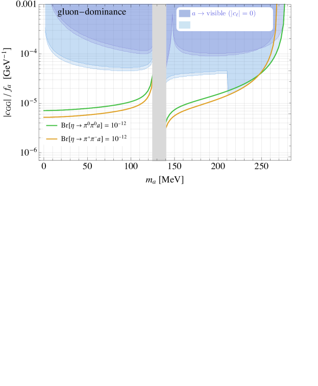
Figure 8: Reach to the ALP parameter space by probes of axio-hadronic $\eta$ decays, such as REDTOP, assuming a branching ratio sensitivity of $\text{Br}[\eta\to\pi\pi a]=10^{-12}$ for all benchmark scenarios. Top panel: gluon dominance scenario, with the green and orange curves denoting the reach to visible^∗ and invisible ALP decays; the dark blue shaded region denoting sensitivity to visible^∗ $a\to\gamma\gamma$ decays of a leptophobic ALP; and the light blue shaded region denoting sensitivity to visible^∗ $a\to\ell^{+}\ell^{-},\gamma\gamma$ decays of a leptophilic ALP.  Bottom panel: analogous to the top panel, but assuming the quark dominance scenario.  ^∗In these plots, the ALP decay is considered visible if the ALP decay vertex is displaced by less than 100 cm from the $\eta$ decay vertex in the $\eta$ rest frame.

Since we are considering ALPs in the context of axio-hadronic $\eta$ decays, they will never be heavy enough to decay hadronically. Therefore, the ALP decay width will be given by:

$$\Gamma_{a}\leavevmode\nobreak\ =\leavevmode\nobreak\ \Gamma(a\to\gamma\gamma)\leavevmode\nobreak\ +\;\sum_{\ell}\;\Gamma(a\to\ell^{+}\ell^{-})\,,$$ (54)

where

$$\Gamma(a\to\gamma\gamma)\leavevmode\nobreak\ =\leavevmode\nobreak\ \frac{m_{a}^{3}}{4\pi}\,\left(\!c_{\gamma\gamma}\;\frac{\alpha}{4\pi f_{a}}\right)^{\!2}\,,$$ (55)

and the sum over lepton flavors in (54) of course only runs over leptons for which the decay $a\to\ell^{+}\ell^{-}$ is kinematically allowed, i.e., for $m_{\ell}<m_{a}/2$, so that

$$\Gamma(a\to\ell^{+}\ell^{-})\leavevmode\nobreak\ =\leavevmode\nobreak\ \frac{m_{a}}{\,8\pi\,}\,\left(\frac{c_{\ell}\,m_{\ell}}{f_{a}}\right)^{\!2}\,\sqrt{1-\frac{4\,m_{\ell}^{2}}{m_{a}^{2}}}\,.$$ (56)

With (51)-(56), we can now complement our definition of the gluon dominance and quark dominance benchmark scenarios in the following way:

• Gluon dominance, leptophobic,

  $$c_{GG}^{\text{\tiny UV}}\neq 0,\leavevmode\nobreak\ \leavevmode\nobreak\ \leavevmode\nobreak\ \leavevmode\nobreak\ c_{q}=0\leavevmode\nobreak\ \forall\leavevmode\nobreak\ q,\leavevmode\nobreak\ \leavevmode\nobreak\ \leavevmode\nobreak\ \leavevmode\nobreak\ c_{\ell}=0\leavevmode\nobreak\ \forall\leavevmode\nobreak\ \ell,\leavevmode\nobreak\ \leavevmode\nobreak\ \leavevmode\nobreak\ \leavevmode\nobreak\ c_{\gamma\gamma}^{\text{\tiny UV}}=0.$$ (57)

• Gluon dominance, flavor universal, leptophilic,

  $$c_{GG}^{\text{\tiny UV}}\neq 0,\leavevmode\nobreak\ \leavevmode\nobreak\ \leavevmode\nobreak\ \leavevmode\nobreak\ c_{q}=0\leavevmode\nobreak\ \forall\leavevmode\nobreak\ q,\leavevmode\nobreak\ \leavevmode\nobreak\ \leavevmode\nobreak\ \leavevmode\nobreak\ c_{\ell}=2c_{GG}^{\text{\tiny UV}}\leavevmode\nobreak\ \forall\leavevmode\nobreak\ \ell,\leavevmode\nobreak\ \leavevmode\nobreak\ \leavevmode\nobreak\ \leavevmode\nobreak\ c_{\gamma\gamma}^{\text{\tiny UV}}=0.$$ (58)

• Quark dominance, flavor universal, leptophobic,

  $$c_{GG}^{\text{\tiny UV}}=0,\leavevmode\nobreak\ \leavevmode\nobreak\ \leavevmode\nobreak\ \leavevmode\nobreak\ c_{q}\neq 0\leavevmode\nobreak\ \forall\leavevmode\nobreak\ q,\leavevmode\nobreak\ \leavevmode\nobreak\ \leavevmode\nobreak\ \leavevmode\nobreak\ c_{\ell}=0\leavevmode\nobreak\ \forall\leavevmode\nobreak\ \ell,\leavevmode\nobreak\ \leavevmode\nobreak\ \leavevmode\nobreak\ \leavevmode\nobreak\ c_{\gamma\gamma}^{\text{\tiny UV}}=0.$$ (59)

• Quark dominance, flavor universal, leptophilic,

  $$c_{GG}^{\text{\tiny UV}}=0,\leavevmode\nobreak\ \leavevmode\nobreak\ \leavevmode\nobreak\ \leavevmode\nobreak\ c_{q}\neq 0\leavevmode\nobreak\ \forall\leavevmode\nobreak\ q,\leavevmode\nobreak\ \leavevmode\nobreak\ \leavevmode\nobreak\ \leavevmode\nobreak\ c_{\ell}=c_{q}\leavevmode\nobreak\ \forall\leavevmode\nobreak\ \ell,\leavevmode\nobreak\ \leavevmode\nobreak\ \leavevmode\nobreak\ \leavevmode\nobreak\ c_{\gamma\gamma}^{\text{\tiny UV}}=0.$$ (60)

Fig. 8 also illustrates the REDTOP sensitivity reach in these four scenarios (shaded regions) assuming a visible branching ratio sensitivity of $\text{Br}[\eta\to\pi\pi(a\to\text{visible})]=10^{-12}$.

III.1.6 Probing a BSM origin of the proton radius anomaly

One of the existing and still unexplained anomalies present in the Standard Model is related to the measurements of the proton radius $R_{p}$ with electron and muon probes.

The processes involved are $\eta$-Dalitz decays, and lepton-pair decays:

$$\eta\rightarrow\gamma e^{+}e^{-}\,,\eta\rightarrow\gamma\mu^{+}\mu^{-}\text{ and }\eta\rightarrow e^{+}e^{-}\,,\eta\rightarrow\mu^{+}\mu^{-}$$ (61)

Other types of $R_{p}$ measurements, using muonic atoms (see, for example, CODATA-2012), or using elastic scattering of electrons and muons on hydrogen atoms, have found a discrepancy corresponding to several sigma in the electron vs muon case. It is worth noting that such processes occur mainly through the exchange of one virtual photon, but subleading corrections to that—needed to better clarify the situation—may include pseudoscalar-exchange contribution to the 2S hyperfine splitting in the muonic hydrogen, in a t-channel contribution. One would expect the $\pi^{0}$ to dominate such subleading correction but being a $t$-channel exchange, all pseudoscalars may contribute, being the processes of the type $\eta(\eta{{}^{\prime}})\rightarrow\gamma l^{+}l^{-}$ a background to them, as shown in Fig. 9 diagram a), versus the two-photon contribution, as shown in Fig. 9 diagram b).

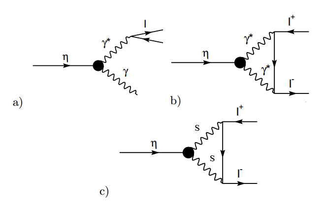
Figure 9: Diagrams contributing to the proton radius

A light scalar particle S with a different coupling with electrons and muons would mediate this process, as shown in diagram c) of figure 9, would explain this anomaly of the Standard Model. Therefore, an experiment able to precisely measure the branching ratios of this particle might help in explaining the $R_{p}$ anomaly.

In REDTOP, the processes (61) are detected simultaneously and within the same experimental apparatus. Consequently, most of the systematic errors are common to the two processes and they factor out in the ratio of the corresponding branching ratios, enhancing the precision of the overall measurement. $\eta^{{}^{\prime}}$ contributions may play a role as well.

III.2 Tests of conservation laws

Conservation laws with their underlying symmetry principles are at the heart of physics, from the classical space-time conservation laws of introductory courses through the symmetries and additive quantum numbers of modern particle physics. The Crystal Ball experiment at the Brookhaven AGS was able to provide a few times $10^{7}$ $\eta$ (as for the $4\pi^{0}$ decay study). It was subsequently moved to MAMI, and a goal there is to achieve another order of magnitude in $\eta$ yield. Other facilities include KLOE (for $\phi(1020)\to\eta\gamma$), and GlueX at JLAB, all at the few times $10^{7}$ level. Recently, WASA at COSY reached a milestone, by collecting about $10^{9}$, although with conventional, background prone, detector technologies, still insufficient for exploring successfully the realm BSM. To reach the more exacting levels needed for symmetry violations, the usable $\eta$ flux must be increased by several orders of magnitude.

To achieve this goal, the REDTOP experiment is being designed to provide a sea change in the number of $\eta$ samples to $1.1\times 10^{14}$ and $\eta^{\prime}$ samples to $1\times 10^{12}$, along with a nearly $4\pi$ detector to study a broad range of fore-front physics. The facility will provide vastly reduced upper limits for $\eta$ and $\eta^{\prime}$ decays, as well as studies of processes that can lead to New Physics Beyond the Standard Model.

The light pseudoscalar mesons $\pi^{0}$, $\eta$, and $\eta^{\prime}$ have very special roles for exploring and testing the conservation laws. The $\pi^{0}$ has a long history of such tests and has established tight upper limits of charge ($C$) and lepton flavor ($LF$) violations et al. (2016). Unlike the isospin $I=1$ for the $\pi^{0}$, all the additive quantum numbers for the $\eta$ and $\eta^{\prime}$ are zero, and they differ from the vacuum only in terms of parity. Due to the opposite $G$ parities of the the $\pi^{0}$ and $\eta$, couplings to strong interactions are suppressed. Thus, tests of $C$ and $CP$ in electromagnetic interactions are much more directly accessible in $\eta$ and $\eta^{\prime}$ decays, limited mainly by the flux of such mesons Nef (1994). In addition, such decays can provide tests of $P$, $T$, $CT$, $PT$, and even $CPT$. Among other possibilities are searches for lepton family violation, leptoquarks, and significant tests of the parameterization of chiral perturbation theory.

Almost all searches for symmetry violations in $\eta$/$\eta^{\prime}$ decays are upper limits in the range of $10^{-5}$ or higher et al. (2016). An exception is the decay $\eta\to 4\pi^{0}$ at $<6.9\times 10^{-7}$, based on $3\times 10^{7}$ $\eta$ mesons Prakhov et al. (2000). One-sigma errors have been reported for some asymmetries in the Dalitz distribution of $\eta\to\pi^{+}\pi^{-}\pi^{0}$ (which are consistent with zero at the level of $10^{-2}$) collaboration et al. (2008). Most models of symmetry violations for various decay processes are at or below the level of $10^{-9}$, typically by several orders of magnitude.

CP violation has been extensively studied in the flavor-changing decays of the neutral $K$- and $B$-mesons. The origin of the violation is still not fully understood. The standard model predicts that the source of CP violation is a single phase in the Cabbibo-Kobayashi-Maskawa (CKM) mixing matrix of quarks couplings. At present, the predictions based on CKM mechanism are consistent with the observations in $K$ and $B$ systems, but tensions are arising. We propose to explore other sources of CP violation beyond the CKM mechanism and with flavor-conserving processes, especially through measurements not bound by EDM limits. Rare $\eta$/$\eta^{\prime}$ decays provide a good laboratory for that. All decays of the $\eta$/$\eta^{\prime}$ mesons into multiple photons or into photons plus $\pi^{0}$s provides a direct test of $C$ invariance. Each photon in the final state, including the two from $\pi^{0}$ decay, has $C=-1$. Because the $\eta$ has $C=+1$, final states with an odd number of photons are forbidden. However, the branching ratio for these processes are bound by EDM measurements and they would explore aspects of CP violations not accessible even at a $\eta$-factory. We propose, instead, studying three processes that are not bound by current EDM measurements and that are probing different operators which would induce a violation of CP from sources Beyond the Standard Model.

Several $\eta$/$\eta^{\prime}$-related processes have been selected to study the sensitivity of REDTOP to Conservation Laws. These studies are restricted, for now, only to the CP violation (CP) and Lepton Flavor violation, where more solid theoretical models exists which are consistent, at the same time, with bounds from EDM measurements and with outstanding experimental anomalies. These are discussed below, alongside with the theoretical models supporting them.

III.2.1 C and CP violation from Dalitz asymmetries in $\eta\rightarrow\pi^{+}\pi^{-}\pi^{0}$

The decay $\eta\to\pi^{+}\pi^{-}\pi^{0}$ can only occur when isospin or/and charge conjugation (C) is/are broken. Thus the interference of a C-conserving but isospin-breaking amplitude with a C-violating one would give rise to a charge asymmetry in the Dalitz plot of the 3$\pi$ final state for this process. Since parity P is conserved in this decay, the existence of a nonzero charge asymmetry would attest to the breaking of C and CP symmetry. In contrast, searches for a nonzero permanent electric dipole moment (EDM) probe the possibility of new sources of P and CP violation. Moreover, the SM mechanism of CP violation, vis-a-vis the flavor-changing weak interactions of quarks, is expected to be completely negligible in this context. Although the charge asymmetry observable was first proposed long ago Lee and Wolfenstein (1965); Nauenberg (1965); Lee (1965), we revisit and refine it not only because it is a flavor-diagonal, C- and CP-violating observable, but it is also, moreover, an effect that scales linearly, rather than quadratically, in the underlying CP-violating parameter Gardner and Shi (2020). Moreover, a study of the new physics sources in Standard Model Effective Field Theory (SMEFT), starting from the compilation of Ref. Grzadkowski et al. (2010), shows that the sources of CP violation that stem from C- or P- violating effects in the flavor diagonal sector are distinct Shi (2020); Gardner and Shi (2022). A charge asymmetry in the $B^{0}(\bar{B}^{0})\to\pi^{+}\pi^{-}\pi^{0}$ Dalitz plot also probes CP violation Gardner and Tandean (2004), and the SMEFT operators in that case are mass dimension six Shi (2020); Gardner and Shi (2022). In our case the SMEFT operators are mass dimension eight, but could be of dimension six in numerical size, which would signal the existence of dynamics beyond SMEFT Shi (2020); Gardner and Shi (2022). (We note Ref. Burgess et al. (2021) for a discussion of analogous ideas in $b\to c\tau\bar{\nu}$ decay.) Thus the measurement of the charge asymmetry in $\eta\to\pi^{+}\pi^{-}\pi^{0}$ decay is an ideal probe with which to explore the possibility of physics beyond the SM. The REDTOP experimental concept is well suited to careful measurements of the charge asymmetry observable, and we consider it a golden channel for study at REDTOP.

Recently, theoretical work has been done Gardner and Shi (2020); Akdag et al. (2022) investigating the patterns of C and CP violation in this process from mirror asymmetry breaking of the Dalitz plot. As long known, when plotting the Dalitz plot in terms of Mandelstam variables $t\equiv(p_{\pi^{-}}+p_{\pi^{0}})^{2}$ and $u\equiv(p_{\pi^{+}}+p_{\pi^{0}})^{2}$, the charge asymmetry would correspond to a breaking of mirror symmetry, i.e., $t\leftrightarrow u$ exchange, in the Dalitz plot. The charge asymmetry can be probed through the measurement of a left-right asymmetry, $A_{LR}$ Layter et al. (1972)

$$A_{LR}\equiv\frac{N_{+}-N_{-}}{N_{+}+N_{-}},$$ (62)

where $N_{\pm}$ is the number of events when $u\stackrel{{\scriptstyle>}}{{{}_{<}}}t$, i.e., the $\pi^{+}$ has more (less) energy than the $\pi^{-}$ in the $\eta$ rest frame. More conveniently, we can describe the Dalitz plot in terms of variables $X$ and $Y$

$$X \equiv \sqrt{3}\frac{T_{\pi^{+}}-T_{\pi^{-}}}{Q_{\eta}}=\frac{\sqrt{3}}{2M_{\eta}Q_{\eta}}(u-t),$$

$$Y \equiv \frac{3T_{\pi^{0}}}{Q_{\eta}}-1=\frac{3}{2M_{\eta}Q_{\eta}}[(M_{\eta}-M_{\pi^{0}})^{2}-s]-1\,,$$ (63)

where $Q_{\eta}=T_{\pi^{+}}+T_{\pi^{-}}+T_{\pi^{0}}=M_{\eta}-2M_{\pi^{+}}-M_{\pi^{0}}$, and $T_{\pi^{i}}$ is the $\pi^{i}$ kinetic energy in the $\eta$ rest frame. The decay amplitude square can be parametrized in a polynomial expansion around $(X,\leavevmode\nobreak\ Y)=(0,\leavevmode\nobreak\ 0)$ Anastasi et al. (2016)

$$|A(s,t,u)|^{2}\! = \!N(1+aY+bY^{2}+cX+dX^{2}+eXY+fY^{3}+gX^{2}Y$$ (64)

$$+ hXY^{2}+lX^{3}+\ldots)\,.$$

The C transformation on the decay is equivalent to $t\leftrightarrow u$ in the amplitude. As a result, the appearance of terms that are odd in $X$ would serve as evidence of C and CP violation in this process Gardner and Tandean (2004); Gardner and Shi (2020).

Although an experimental determination of non-zero coefficients for the terms with odd powers of $X$ ($c$,$e$,$h$) in the study of the $\eta\to\pi^{+}\pi^{-}\pi^{0}$ Dalitz plot would signal both $C$ and $CP$ violation, it is possible to gain insight into the isospin structure of the new physics sources through consideration of their chiral dynamics. We follow Ref. Gardner and Shi (2020) for our discussion. The decay amplitude in the SM, working to leading order in isospin breaking, can be expressed as Gasser and Leutwyler (1985); Anisovich and Leutwyler (1996)

$$A(s,t,u) = -\frac{1}{Q^{2}}\frac{M_{K}^{2}}{M_{\pi}^{2}}\frac{M_{K}^{2}-M_{\pi}^{2}}{3\sqrt{3}F_{\pi}^{2}}M(s,t,u)\,.$$ (65)

Since $C=-(-1)^{I}$ in $\eta\to 3\pi$ decay Lee (1965), the C- and CP-even transition amplitude with a $\Delta I=1$ isospin-breaking prefactor must have $I=1$. The amplitude $M(s,t,u)$ thus corresponds to the total isospin $I=1$ component of the $\pi^{+}\pi^{-}\pi^{0}$ state and can be expressed as Anisovich and Leutwyler (1996); Lanz (2011)

$$M^{C}_{1}\!(s,t,u) = M_{0}^{0}(s)+(s-u)M_{1}^{1}(t)+(s-t)M_{1}^{1}(u)$$ (66)

$$+ M_{2}^{0}(t)+M_{2}^{0}(u)-\frac{2}{3}M_{2}^{0}(s)\,,$$

where $M_{I}^{\ell}$(z) is an amplitude with $\pi-\pi$ rescattering in the $z$-channel with isospin $I$ (and orbital angular momentum $\ell$). We refer to Sec. IVA for a nuanced discussion of their construction, pertinent to a high-precision extraction of the light quark mass difference. The decomposition can be recovered under isospin symmetry in chiral perturbation theory (ChPT) up to next-to-next-to-leading order (NNLO), ${\cal O}(p^{6})$, because the only absorptive parts that can appear are in the $\pi-\pi$ $S-$ and $P$-wave amplitudes Bijnens and Ghorbani (2007).

Since we are considering C and CP violation, additional amplitudes can appear — namely, total $I=0$ and $I=2$ amplitudes. The complete amplitude is thus

$$A(s,t,u) = -\frac{1}{Q^{2}}\frac{M_{K}^{2}}{M_{\pi}^{2}}\frac{M_{K}^{2}-M_{\pi}^{2}}{3\sqrt{3}F_{\pi}^{2}}M^{C}_{1}\!(s,t,u)$$ (67)

$$+\alpha M^{\not C}_{0}\!(s,t,u)+\beta M^{\not C}_{2}\!(s,t,u)\,,$$

where $\alpha$ and $\beta$ are unknown, low-energy constants — complex numbers to be determined by fits to the experimental event populations in the Dalitz plot. If they are determined to be non-zero, they signal the appearance of C- and CP-violation. Following the expectations of Watson’s theorem Watson (1954); Gardner et al. (2001) we write Gardner and Shi (2020)

$$\!\!M^{\not C}_{0}\!(s,t,u)\!=\!(s-t)\!M_{1}^{1}(u)+(u-s)\!M_{1}^{1}(t)-(u-t)\!M_{1}^{1}(s)$$ (68)

and

$$\!\!\!\!\!\!M^{\not C}_{2}\!(s,t,u)\! = \!(s-t)M_{1}^{1}(u)+(u-s)M_{1}^{1}(t)$$ (69)

$$\!\!\!+2(u-t)M_{1}^{1}(s)+\sqrt{5}[M_{2}^{0}(u)-M_{2}^{0}(t)]\,.$$

In what follows we adopt the NLO analyses of Refs. Gasser and Leutwyler (1985); Bijnens and Ghorbani (2007) to construct particular forms for the $M_{I}^{\ell}$ and refer to Ref. Gardner and Shi (2020) for all details. The analysis we have outlined here has been employed in the sensitivity analysis of Sec. XIII. We emphasize that the normalization factor $N$ as in Eq. (64) drops out in the experimental asymmetry $A_{LR}$, Eq. (62).

Besides, it is also possible to measure the asymmetries which can probe the isospin of the CP violating final state: a sextant asymmetry $A_{S}$ which is sensitive to the $I=0$ state Lee (1965); Nauenberg (1965) and a quadrant asymmetry which is sensitive to the $I=2$ final state Lee (1965); Layter et al. (1972), which are illustrated in Fig. 10. However, an alternate, more sensitive discriminant of the isospin structure of the new CP-violating sources can be found by studying the pattern of the Dalitz plot in realizing the left-right asymmetry, Eq. (62) Gardner and Shi (2020). See also Ref. Akdag et al. (2022) for a comparison of $C$-violating effects of different isospin in similar $\eta^{\prime}$ three-body decays.

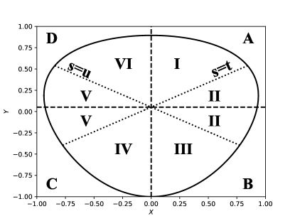
Figure 10: The Dalitz plot geometry in $\eta\to\pi^{+}\pi^{-}\pi^{0}$ decay, split into regions for probes of its symmetries. The solid line is the boundary of the physically accessible region. The asymmetry $A_{LR}$, Eq. (62), compares the population $N_{+}$ ($X>0$) with $N_{-}$ ($X<0$). The quadrant asymmetry $A_{Q}$ probes $I=2$ contributions, $N_{\rm tot}A_{Q}\equiv N({\rm A})+N({\rm C})-N({\rm B})-N({\rm D})$ Lee (1965), and the sextant asymmetry $A_{S}$ probes $I=0$ contributions, $N_{\rm tot}A_{S}\equiv N({\rm I})+N({\rm III})+N({\rm V})-N({\rm II})-N({\rm IV})-N({\rm VI})$ Barrett et al. (1966); Lee (1965). All asymmetries probe C and CP violation. Figure from Ref. Gardner and Shi (2020).

Analysis of the data is complex. Monte Carlo calculations must include adjustments for experimental efficiencies and $\pi\pi$ interactions. The results for the left-right (LR or $X$), quadrant (Q), and sextant (S) asymmetries for $1.34\times 10^{6}$ $\eta\to\pi^{+}\pi^{-}\pi^{0}$ decays collaboration et al. (2008) are:

$$A_{LR} = (+0.09\pm 0.10\,_{-0.14}^{+0.10})\times 10^{-2}$$

$$A_{Q} = (-0.05\pm 0.10\,_{-0.05}^{+0.05})\times 10^{-2}$$

$$A_{S} = (+0.08\pm 0.10\,_{-0.13}^{+0.08})\times 10^{-2}$$ (70)

Observation of statistically significant asymmetries would be an evidence of $C$ and $CP$ violation. REDTOP is particularly suitable for this measurement since the reconstruction of charged pions in a Optical-TPC does not rely on a magnetic field, which is usually the largest source of systematic asymmetries. Therefore, it can vastly improve the accuracy of the measurements and resolve the discrepancies.

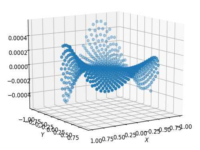
Figure 11: 3-D representation of the Dalitz plot for the $\eta\rightarrow\pi^{+}\pi^{-}\pi^{0}$ process.

A 3-dimensional representation of the X and Y variables for the $\eta\to\pi^{+}\pi^{-}\pi^{0}$ process is shown in Fig. 11. The appearance of terms that are odd in X would indicate both C and CP violation. The detection of charged pions in REDTOP is based on the measurement of the Cerenkov angle of the photons radiated in the aerogel (cf. Sec. VI.4.2). Therefore, the non-uniformity of the magnetic field, which in general corresponds the largest contribution to the systematic error in the asymmetry of kinematics variables of positive and negative charged particles, plays no role at REDTOP. The expected sensitivity for this process is currently under study with the REDTOP detector, although it is expected to be higher than that with more traditional, magnetic spectrometers.

III.2.2 CP violation in $\eta\rightarrow\pi^{+}\pi^{-}e^{+}e^{-}$

P and CP violation in the decay of $\eta\to\pi^{+}\pi^{-}\gamma$ has been discussed nearly fifty years before Herczeg and Singer (1973). More recent study Geng et al. (2002) has analyzed the CP-violating effects in this decay by considering the photon polarizations, and predicted that a sizable linear photon polarization could be expected in some new physics scenarios. In order to avoid measuring the photon polarization, one can consider, as shown in Ref. Gao (2002), the decay $\eta\rightarrow\pi^{+}\pi^{-}e^{+}e^{-}$ resulting from the internal conversion of the photon into an $e^{+}e^{-}$ pair, and the CP-violating effects hidden in the polarization of the photon now can be translated into the CP asymmetry in the angular correlation of the $e^{+}e^{-}$ plane relative to the $\pi^{+}\pi^{-}$ plane. This is actually analogous to the neutral $K$ system, in which a large CP asymmetry, due to the interference between the parity-conserving magnetic amplitudes and the parity-violating electric amplitudes of $K_{L}\rightarrow\pi^{+}\pi^{-}\gamma^{*}\rightarrow\pi^{+}\pi^{-}e^{+}e^{-}$, has already been predicted theoretically and confirmed experimentally. Thus the asymmetry in $\eta\rightarrow\pi^{+}\pi^{-}e^{+}e^{-}$ transition could be found by analyzing its angular distribution Gao (2002), which is given by

$${A}_{\phi}=\langle sign(\sin\phi\cos\phi)\rangle=\frac{\displaystyle\int_{0}^{2\pi}\frac{d\Gamma(\eta\rightarrow\pi^{+}\pi^{-}e^{+}e^{-})}{d\phi}d\phi\leavevmode\nobreak\ sign(\sin\phi\cos\phi)}{\displaystyle\int_{0}^{2\pi}\frac{d\Gamma(\eta\rightarrow\pi^{+}\pi^{-}e^{+}e^{-})}{d\phi}d\phi},$$ (71)

where $\phi$ is the angle between the $e^{+}e^{-}$ and $\pi^{+}\pi^{-}$ planes in the $\eta$ rest frame (see Fig. 63).

It is obvious that the asymmetry in the flavor-conserving $\eta\rightarrow\pi^{+}\pi^{-}e^{+}e^{-}$ decay, different from flavoring-changing processes like $K_{L}\rightarrow\pi^{+}\pi^{-}e^{+}e^{-}$, indicates the presence of non-standard CP-violation. It has been shown in Geng et al. (2002); Gao (2002) that this asymmetry will arise if a relevant parity-violating electric transition exists, and such manifestation of CP violation in some New Physics scenarios might not be bounded by existing EDM measurements; cf. however the discussion in Ref. Gan et al. (2022).

Experimentally, the first measurement of such asymmetry has been done by the KLOE Collaboration in 2009 Ambrosino et al. (2009). The current best measurement has been performed by the WASA-at-COSY Collaboration Adlarson et al. (2016) and it is consistent with zero. However, the statistical error (based on the production of $\sim 10^{9}$ $\eta$-mesons) largely dominates the measurement. REDTOP’s larger statistics will improve on the systematic error by almost two orders of magnitude, bringing the sensitivity to a level where CP-violation could be observed. Thus, further experimental investigation of this asymmetry might be helpful to increase our knowledge on CP violation, or to impose some interesting constraints on some theoretical models.

Similar work can be directly generalized to $\eta/\eta^{\prime}\to\pi^{+}\pi^{-}\ell^{+}\ell^{-}$ decays including $\ell=e,\mu$. Very recently, the experimental measurement of such asymmetry in $\eta^{\prime}\to\pi^{+}\pi^{-}e^{+}e^{-}$ has been performed by the BESIII Collaboration Ablikim et al. (2021).

III.2.3 Tests of CP invariance via $\gamma^{*}$ polarization studies in $\eta\to\pi^{+}\pi^{-}\gamma^{*}$

CP-violation can also be investigated with a virtual photon decaying into a lepton-antilepton pair, as in

$$\eta\rightarrow\pi^{+}\pi^{-}\gamma^{*}\quad\text{with}\quad\gamma^{*}\rightarrow l^{+}+l^{-},$$ (72)

by considering the asymmetry

$$A_{\Phi}=\frac{N(\sin\phi\cos\phi>0)-N(\sin\phi\cos\phi<0)}{N(\sin\phi\cos\phi>0)+N(\sin\phi\cos\phi<0)}$$ (73)

where $\phi$ is the angle between the decay planes of the lepton-antilepton pair and the two charged pions. CP invariance requires $A_{\Phi}$ to vanish. At the present, the measurement of such asymmetry performed by the WASA collaboration Adlarson et al. (2015) is the best available, and it is consistent with zero within the measurement errors. Unfortunately, that measurement is largely dominated by the statistical error, from the production of only $\sim 10^{9}\>\eta$-mesons. The larger statistics of REDTOP will improve the systematic error by almost two orders of magnitude.

III.2.4 CP violation in $\eta\to\mu^{+}\mu^{-}$

The most general amplitude for $\eta\to\ell^{+}\ell^{-}$ can be effectively parametrized as

$$\mathcal{M}=g_{P}(\bar{u}i\gamma^{5}v)+g_{S}(\bar{u}v),$$ (74)

with $g_{P,S}$ dimensionless parameters. The first contribution is $CP$ even and has been computed in the SM (see Sanchez-Puertas (2019); Masjuan and Sanchez-Puertas (2016) and references therein), while the latter represents a $P$-odd $C$-even contribution, that is negligible in the SM. As such, any indication of a nonzero $g_{S}$ would be a clear signal of New Physics. A possible way to access this is through $CP$-odd lepton polarization observables, that are of order $\mathcal{O}(g_{S}g_{P})$ and require of muon polarimetry techniques — otherwise, the first contribution appears at $\mathcal{O}(g_{S}^{2})$. A general caveat of these searches is that, in general, $P$-odd $C$-even observables are tightly bound by neutron and lepton EDMs, that make such a positive finding a priori unexpected at any foreseeable meson factory. An exception to this was found in Ref. Sanchez-Puertas (2019), where the New Physics were studied using the SMEFT D=6 operators. There it was shown that, while EDM operators (or hadronic $CP$-odd operators inducing $CP$-violating transition form factors) are severely constrained by neutron and lepton EDMs, quark-lepton Fermi operators are less severely constrained for the case of muons (additional constraints exists for electrons Yanase et al. (2019)). As such, we foucs in the latter scenario which is the most appealing case (find comments regarding $CP$-violating TFFs in double-Dalitz decays, Sect. III.2.5). In particular, the single operators of such kind inducing $CP$-violation are $\mathcal{O}_{\ell equ}^{(1)}$ and $\mathcal{O}_{\ell edq}$ Grzadkowski et al. (2010), whose EDM contribution starts at two loops, providing the necessary suppression to avoid EDM constraints.

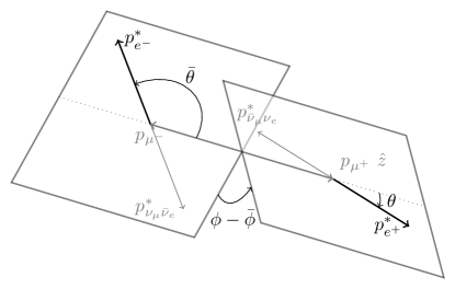
Figure 12: Kinematics of the process. The decaying muons’ momenta in the $\eta$ rest frame are noted as $p_{\mu^{\pm}}$, while the $e^{\pm}$ momenta, $p^{*}_{e^{\pm}}$, is shown in the corresponding $\mu^{\pm}$ reference frame along with the momenta of the $\nu\bar{\nu}$ system. The $\hat{z}$ axis is chosen along $p_{\mu^{+}}$.

Ref. Sanchez-Puertas (2019) introduced two different muon’s polarization asymmetries,

$$A_{L}=\frac{N(\cos\theta>0)-N(\cos\theta<0)}{N}=\operatorname{Im}[4.1c_{\ell edq}^{2222}-2.7(c_{\ell equ}^{(1)2211}+c_{\ell edq}^{2211})]\times 10^{-2},$$ (75)

$$A_{\times}=\frac{N(\sin\Phi>0)-N(\sin\Phi<0)}{N}=\operatorname{Im}[2.5c_{\ell edq}^{2222}-1.6(c_{\ell equ}^{(1)2211}+c_{\ell edq}^{2211})]\times 10^{-3},$$ (76)

with the first one identical if replacing $\theta\to\bar{\theta}$. Above, $\theta(\bar{\theta})$ represents the polar angle of the $e^{+}(e^{-})$ in the $\mu^{+}(\mu^{-})$ reference frame, with the $\hat{z}$ axis fixed by the $\mu^{+}$ direction in the $\eta$ rest frame, see Fig. 12. The angle $\Phi=\phi-\bar{\phi}$ is defined in Fig. 12 and reflects the sign of $(\vec{p}_{e^{-}}\times\vec{p}_{e^{+}})\cdot\vec{p}_{\mu^{+}}$. The right hand side in the equations above provides the contribution from the aforementioned operators, with $c_{\mathcal{O}}^{(llqq)}$ the corresponding Wilson coefficient for the $l(q)$-th lepton(quark) generation, respectively. The nEDM bounds derived in Ref. Sanchez-Puertas (2019) (bounds from $D_{s}$ decays analyzed in Ref. Sanchez-Puertas (2021) are similar, but less severe) updated with the most recent nEDM measurement Abel et al. (2020) imply

$$\operatorname{Im}c_{\ell equ}^{(1)2211}<0.001,\operatorname{Im}c_{\ell edq}^{2211}<0.008,\operatorname{Im}c_{\ell edq}^{2222}<0.02.$$ (77)

Clearly, the highest sensitivity happens for the coefficient involving muons and strange quarks, $c_{\ell equ}^{(1)2222}$, and sets the target sensitivity at REDTOP since one expects $A_{L}<10^{-3}$ from the bounds above.

III.2.5 CP violation in double Dalitz decays $\eta\to\ell^{+}\ell^{-}\ell^{\prime+}\ell^{\prime-}$

Similar to $\eta\to\mu^{+}\mu^{-}$ decays, Ref. Sanchez-Puertas (2019) showed that $CP$ violation effects encoded in either quark/lepton EDM as well as in $CP$-violating hadronic operators driving $CP$-odd transition form factors are unexpected due to EDM bounds. In addition, the sensitivity to quark-lepton $CP$ violating interactions was studied there, while this involves an $\alpha$ suppression with respect to the $\eta\to\mu^{+}\mu^{-}$ case that arises from the $e^{+}e^{-}$ emission: $\eta\to\mu^{+}\mu^{-}\to\mu^{+}\mu^{-}\gamma^{*}\to\mu^{+}\mu^{-}e^{+}e^{-}$. In particular, the contribution to the asymmetry was expressed as

$$A_{\sin\phi\cos\phi}=\operatorname{Im}[1.9c_{\ell edq}^{2222}-1.3(c_{\ell equ}^{(1)2211}+c_{\ell edq}^{1122})]\times 10^{-5}-0.2\epsilon_{1}+0.0003\epsilon_{2}$$ (78)

where $c_{\mathcal{O}}$ are the corresponding Wilson coefficients introduced in Sect. (III.2.4) and $\epsilon_{1,2}$ characterizes the coupling strength of the $CP$-violating TFFs in Eq. (89), see Sanchez-Puertas (2019). Once more, nEDM put constraints on these. In particular, Ref. Sanchez-Puertas (2019) showed that, necessarily, $\epsilon_{1}<3\times 10^{-7}$; $\epsilon_{2}$ is unconstrained, but there is no theoretical motivation for having $\epsilon_{2}\gg\epsilon_{1}$ (further, possibly more stringent bounds could be derived if the microscopic origin of $CP$ violation is specified). Still, we include them for completeness, as it is the most competitive channel to access $\epsilon_{1}$.

III.2.6 CP violation in $\eta\rightarrow\pi^{0}\mu^{+}\mu^{-}$

Yet another opportunity to search for violation of discrete symmetries is found in the $\eta\to\pi^{0}\mu^{+}\mu^{-}$ decay. It is useful to parametrize the corresponding matrix element as Escribano et al. (2022a)

$$\mathcal{M}=m_{\mu}(\bar{u}v)F_{1}(q^{2},\bar{q}\cdot k)+(\bar{u}i\gamma^{5}v)F_{2}(q^{2},\bar{q}\cdot k)+(\bar{u}\not{k}v)F_{3}(q^{2},\bar{q}\cdot k)+i(\bar{u}\not{k}\gamma^{5}v)F_{4}(q^{2},\bar{q}\cdot k)\ ,$$ (79)

with $q=p_{\mu^{+}}+p_{\mu^{-}}$, $\bar{q}=p_{\mu^{+}}-p_{\mu^{-}}$, $k=p_{\eta}+p_{\pi^{0}}$, and the form factors $F_{i}(q^{2},\bar{q}\cdot k)$. With these definitions, $F_{1,2}(q^{2},\bar{q}\cdot k)$ are $P$ even whereas $F_{3,4}(q^{2},\bar{q}\cdot k)$ are $P$ odd. In addition, a $C$ transformation effectively amounts to $F_{1,2,4}(q^{2},\bar{q}\cdot k)\to F_{1,2,4}(q^{2},-\bar{q}\cdot k)$ and $F_{3}(q^{2},\bar{q}\cdot k)\to-F_{3}(q^{2},-\bar{q}\cdot k)$. The SM contribution to the above process is vastly dominated by the electromagnetic interactions (thus, $CP$ even) and produces non-vanishing form factors for $i=1,2$, with $F_{1(2)}(q^{2},\bar{q}\cdot k)$ an even(odd) function of $(\bar{q}\cdot k)$, see Refs. Escribano et al. (2022a); Escribano and Royo (2020) and references therein.

The $\eta\to\pi^{0}\mu^{+}\mu^{-}$ process is a great testing ground for BSM searches, such as, for example, $P$-odd, $C$-even new-physics effects. In particular, with 3 particles in the final state, this necessarily involves polarization observables, in line with $\eta\to\mu^{+}\mu^{-}$ decays, see Sect. (III.2.4). The possibility of testing $P$-odd, $C$-even contributions was studied in Ref. Escribano et al. (2022a) using the SMEFT as the general framework to capture physics BSM. Much in the same way as in Sect. (III.2.4), the less constrained contributions originate from quark-lepton Fermi operators, whose EDM bounds are far less constrained. Specifically, the main contributions arise from the same operators appearing in $\eta\to\mu^{+}\mu^{-}$ decays and are associated to the scalar matrix elements

$$F_{2}=\left[\operatorname{Im}c_{\ell edq}^{2211}\langle 0|\bar{d}d|\eta\pi^{0}\rangle+\operatorname{Im}c_{\ell edq}^{2222}\langle 0|\bar{s}s|\eta\pi^{0}\rangle-\operatorname{Im}c_{\ell equ}^{(1)2211}\langle 0|\bar{u}u|\eta\pi^{0}\rangle\right]\!/v^{2}\ ,$$ (80)

that were computed in Ref. Escribano et al. (2022a) within the framework of large-$N_{c}$ $\chi$PT. Note, in particular, that the second matrix element in Eq. (80) vanishes in the isospin limit. Once again, the key polarisation observables are those defined in Eqs. (75,76). Using input from Ref. Escribano and Royo (2020), the final results for the asymmetries read

$$A_{L}^{\eta\to\pi^{0}\mu^{+}\mu^{-}} {}\!=-0.19(6)\operatorname{Im}c_{\ell equ}^{(1)2211}-0.19(6)\operatorname{Im}c_{\ell edq}^{2211}-0.020(9)\operatorname{Im}c_{\ell edq}^{2222}\ ,$$ (81)

$$A_{\times}^{\eta\to\pi^{0}\mu^{+}\mu^{-}} {}\!=0.07(2)\operatorname{Im}c_{\ell equ}^{(1)2211}+0.07(2)\operatorname{Im}c_{\ell edq}^{2211}+7(3)\times 10^{-3}\operatorname{Im}c_{\ell edq}^{2222}\ .$$ (82)

The comparatively larger suppression for the $s$-quark contribution arises from isospin breaking, that is an $\mathcal{O}(1\%)$ effect, and reduces the sensitivity as compared to $\eta\to\mu^{+}\mu^{-}$ decays. Current nEDM bounds imply for the above asymmetries that $A_{L}<4\times 10^{-4}$ and $A_{\times}<1.4\times 10^{-4}$, which should be contrasted with the REDTOP capabilities.

III.2.7 Lepton flavor violation measurements

This study is motivated by a recent work on decays of quarkonium states M with different quantum numbers Hazard and Petrov (2018, 2016a). The model could be used to put constraints on the Wilson coefficients of effective operators describing LFV interactions at low energy scales. Furthermore, studies of radiative lepton flavor violating meson decays could provide important complementary access to specific effective operators. REDTOP will be able to probe the model with the processes: $\eta/\eta^{\prime}\rightarrow e^{+}\mu^{-}+c.c.$ and $\eta/\eta^{\prime}\rightarrow\gamma\,e^{+}\mu^{-}+c.c.$ This study has been planed for the Snowmass-2022 Summer exercise.

III.2.8 Tests of lepton flavor universality with $\eta/\eta^{\prime}$ mesons

For definiteness let us consider the purely leptonic decay $\eta/\eta^{\prime}\to\ell^{+}\ell^{(\prime)-}$, starting from the case of leptons of equal flavour. Given the amplitude for such decays, its imaginary and real parts are bounded separately. The former can be unambiguously related to the $\eta\to\gamma\gamma$ decay rate, which is measured. This provides the so-called “unitarity bound”, which is quoted from Dre ; Berman and Geffen (1960); Geffen and Young (1965) as Abegg et al. (1994)

$$\Gamma(P\to\ell^{+}\ell^{-})\geq\frac{\alpha^{2}}{2\beta}\left[\left(\frac{m_{\ell}}{m_{P}}\right)\ln\left(\frac{1+\beta}{1-\beta}\right)\right]^{2}\times\Gamma(P\to\gamma\gamma)\leavevmode\nobreak\ ,$$ (83)

with $P$ denoting either of $\eta,\eta^{\prime}$ and $\beta=\sqrt{1-4m_{\ell}^{2}/m_{P}^{2}}$.

The real part depends on the $P\to\gamma\gamma$-vertex form factor, which is estimated within quark models or vector meson dominance, and thus involves non-systematic theoretical assumptions. These calculations return values that are typically 30% larger than the unitarity lower limit Landsberg (1985). This contribution may be affected by New Physics, for example $t$-channel exchange of a leptoquark, whereby the two quark-lepton currents give rise to the external states in an obvious way. One finds Mayer (1990) that values for the ratio of mass to coupling constant below several hundred GeV can be excluded for transitions within the 1st generation. For transitions between different generations the excluded region reaches up to 200 TeV based on the upper limit for BR($K_{L}\to ee$).

The case of leptons with different flavour has the huge advantage of being a null test in the SM. In this case one may consider decays to $\geq 2$ final states, including $\eta^{(\prime)}\to\mu^{\pm}e^{\mp}(\gamma\mbox{\leavevmode\nobreak\ or\leavevmode\nobreak\ }\pi^{0})$ as well as $\eta^{\prime}\to\eta\mu^{\pm}e^{\mp}$. These decays have been discussed specifically in Ref. Hazard and Petrov (2016b). Although these decays would not directly probe the LFV couplings hinted at by the “$B$ anomalies” (see discussion in Glashow et al. (2015); Guadagnoli and Lane (2015)) the probed couplings may actually be related to those from the $B$ anomalies by general effective-theory arguments plus minimal flavour assumptions Borsato et al. (2019). With this in mind, and as shown in table 7 of Ref. Hazard and Petrov (2016b), the constraints placed on the magnitude of LFV $c/\Lambda^{2}$ couplings range between a few $\times 10^{-3}$ and $10^{4}$ GeV^-2. For natural, O(1) WCs this implies that the natural effective scale probed is between about 20 GeV and 6 MeV. Actually, the very same LFV couplings probed by the above decays are also probed by $\mu\to e$ conversion in nuclei, which yields bounds stricter by several orders of magnitude. Ref. Gan et al. (2022) actually suggests to use the latter to constrain $\eta$ and $\eta^{\prime}$ decays, by invoking $\eta^{(\prime)}$ exchange mechanisms, and at the price of the ensuing model dependence.

Another set of potential probes of high-energy New Physics are ratios of $\eta$ or $\eta^{\prime}$ decays to $X\ell^{+}\ell^{-}$, where $\ell$ is different between the numerator and the denominator and $X$ denotes additional final-state particle(s). Such ratios would probe lepton universality. A few considerations are in order however. First, decays induced by the weak interaction are extremely rare, below $10^{-10}$, and thus well below, by many orders of magnitude, existing experimental upper limits. The purely leptonic case is, as mentioned, dominated by intermediate di-photon exchange, and the suppression of this SM mechanism would suggest these decays as good probes of BSM effects. In practice, even assuming tree-level New Physics, modifications to the SM amplitude have to be small, because $Z$-boson exchange per se modifies the rate at the per mil level. Handy formulae can be found in Ref. Gan et al. (2022). As a consequence, again, these ratios are way more suited as probes of light, GeV-scale or below, New Physics.

IV Non-perturbative QCD

Studying the decays of $\eta$ and $\eta^{\prime}$ mesons open a window into the complex QCD dynamics at low energies. For recent reviews on the subject, see e.g. Gan et al. (2022); Albaladejo et al. (2021). At these energies, ($m_{\eta}\sim 548$ MeV and $m_{\eta^{\prime}}\sim 958$ MeV) strong interactions become non-perturbative and the usual series expansion in the strong coupling constant does not provide an appropriate theoretical framework. One has to instead rely on non-perturbative techniques such as effective field theory—Chiral Perturbation Theory ($\chi$PT) for light quarks—, dispersion relations, or numerical simulations such as lattice QCD.

The $\eta$ meson is very peculiar: its main decay channel $\eta\to 3\pi$ violates G-parity, thereby providing an unique access to the light quark masses. It also allows one to test the $\chi PT$ framework and complement it with the dispersive methods.

The description of $\eta^{\prime}$ decays poses additional challenges. In particular, it requires an extension of the $\chi PT$ framework, many aspects of which still remain to be worked out.

The REDTOP experiment with the expected $10^{14}$ $\eta$ and $10^{12}$ $\eta^{\prime}$ will provide crucial data to advance this endeavor to the next level of precision.

IV.1 $\eta\to 3\pi$ and light quark mass extraction

The process $\eta\to 3\pi$ is very interesting because since this decay is forbidden by isospin symmetry—three pions cannot combine to a system with vanishing angular momentum, zero isospin, and even $C$-parity—it offers an unique experimental access to the light quark mass ratio

$$Q^{2}=\frac{m_{s}^{2}-\hat{m}^{2}}{m_{d}^{2}-m_{u}^{2}}\quad\text{where}\quad\hat{m}=\frac{m_{u}+m_{d}}{2}.$$ (84)

The decay width of $\eta\to 3\pi$ can be seen as a measure for the size of isospin breaking in QCD. This is the case because the electromagnetic isospin-breaking effects have been shown to be small Bell and Sutherland (1968); Sutherland (1966); Baur et al. (1996); Ditsche et al. (2009).

The extraction of $Q$ is done by comparing the experimental measured decay width with the reduced amplitude $M(s,t,u)$ integrated over the phase space:

$$\Gamma\big{(}\eta\to\pi^{+}\pi^{-}\pi^{0}\big{)}=\frac{1}{Q^{4}}\frac{M_{K}^{4}(M_{K}^{2}-M_{\pi}^{2})^{2}}{6912\pi^{3}M_{\eta}^{3}M_{\pi}^{4}F_{\pi}^{4}}\int_{s_{\rm min}}^{s_{\rm max}}ds\int_{u_{-}(s)}^{u_{+}(s)}du\left|M(s,t,u)\right|^{2}\,,$$ (85)

with $s\equiv(p_{\pi^{+}}+p_{\pi^{-}})^{2}$, $t\equiv(p_{\pi^{-}}+p_{\pi^{0}})^{2}$, and $u\equiv(p_{\pi^{+}}+p_{\pi^{0}})^{2}$, the so-called Mandelstam variables. The aim is to compute the amplitude $M(s,t,u)$ with the highest possible accuracy.

This is not an easy task since there are strong rescattering effects among the final-state pions. These were initially calculated perturbatively in $\chi$PT. The current algebra or leading order (LO) result in $\chi$PT gives $\Gamma(\eta\to\pi^{+}\pi^{-}\pi^{0})_{\text{LO}}=66$ eV Osborn and Wallace (1970). It receives a substantial enhancement $\Gamma(\eta\to\pi^{+}\pi^{-}\pi^{0})_{\text{NLO}}=160(50)$ eV Gasser and Leutwyler (1985) due to chiral one-loop corrections. The NLO result is still far from the experimental value $\Gamma(\eta\to\pi^{+}\pi^{-}\pi^{0})=300\pm 12$ eV Zyla et al. (2020a) suggesting a convergence problem. Moreover, it has been shown that the two-loop or NNLO calculation Bijnens and Ghorbani (2007) may lead to a precise numerical prediction only after the low-energy constants (LECs) appearing in the amplitude are determined reliably. In particular, the role played by the $\mathcal{O}(p^{6})$ LECs is non-negligible and they are largely unknown.

A more accurate approach relies on dispersion relations to evaluate rescattering effects to all orders Anisovich (1995); Anisovich and Leutwyler (1996); Kambor et al. (1996); Walker (1998). This is not completely independent of $\chi$PT, because the dispersive representation requires the subtraction constants as input, and they can be calculated in $\chi$PT.

There has been a renewed interest in $\eta\to 3\pi$ dispersive analyses due to new and more precise measurements of this decay. In particular recent measurements of the Dalitz plot of the charged ($\eta\to\pi^{+}\pi^{-}\pi^{0}$) channel by KLOE Ambrosino et al. (2008); Anastasi et al. (2016) and BESIII Ablikim et al. (2015a) and of the neutral channel ($\eta\to\pi^{0}\pi^{0}\pi^{0}$) by A2 Prakhov et al. (2018) have achieved an impressive level of precision. New measurements are planned by BESSIII and at JLab by GlueX Gan et al. (2014); Gan (2015) and CLAS Amaryan (2013), with completely different systematics and even better accuracy. Given its unprecedented statistics, REDTOP could definitely play a crucial role in measuring this decay.

The amplitude $M(s,t,u)$ in Eq. (85) is determined using the dispersion-theoretical Khuri–Treiman equations Khuri and Treiman (1960); Aitchison and Pasquier (1966). In this framework, a set of integral equations for the scattering process $\eta\pi\to\pi\pi$ is established before being analytically continued to describe the decay $\eta\to 3\pi$. The amplitude is decomposed in terms of single-variable functions neglecting $D$-and higher waves:

$$M(s,t,u)=M_{0}^{0}(s)+(s-u)M_{1}^{1}(t)+(s-t)M_{1}^{1}(u)+M_{2}^{0}(t)+M_{2}^{0}(u)-\frac{2}{3}M_{2}^{0}(s)\,.$$ (86)

The functions $M_{I}^{\ell}(s)$ have isospin $I$ and angular momentum $\ell$. In the context of light mesons, this decomposition is commonly referred to as a reconstruction theorem Stern et al. (1993); Knecht et al. (1995); Ananthanarayan and Buettiker (2001); Zdrahal and Novotny (2008). The latter relies on the observation that up to corrections of order $\mathcal{O}(p^{8})$ (or three loops) in the chiral expansion, partial waves of any meson–meson scattering process with angular momentum $\ell\geqslant 2$ contain no imaginary parts. The splitting of the full amplitude into these single-variable functions is not unique: there is some ambiguity in the distribution of the polynomial terms over the various $M_{I}^{\ell}$ due to $s+t+u=m_{\eta}^{2}+m_{\pi^{+}}^{2}+m_{\pi^{-}}^{2}+m_{\pi^{0}}^{2}$ being constant.

The use of analyticity and unitarity allows one to construct dispersion relations for the single-variable functions $M_{I}^{\ell}(s)$, and one arrives to

$$M_{I}^{\ell}(s) =\Omega_{I}^{\ell}(s)\left\{P_{I}(s)+\frac{s^{n_{I}}}{\pi}\int_{4m_{\pi}^{2}}^{\infty}\frac{\text{d}s^{\prime}}{s^{\prime n_{I}}}\frac{\sin\delta_{I}^{\ell}(s^{\prime})\hat{M}^{\ell}_{I}(s^{\prime})}{|\Omega_{I}^{\ell}(s^{\prime})|(s^{\prime}-s-i\epsilon)}\right\},$$ (87a)

$$\hat{M}_{I}^{\ell}(s) =\sum_{n,I^{\prime}}\int_{-1}^{1}\text{d}\cos\theta\leavevmode\nobreak\ \cos^{n}\theta\,c_{nII^{\prime}}M_{I^{\prime}}^{\ell}\big{(}t(s,\cos\theta)\big{)}\leavevmode\nobreak\ ,$$ (87b)

where $\hat{M}_{I}^{\ell}(s)$ represents the left-handed cuts. The explicit forms of the coefficients $c_{nII^{\prime}}$ can be found e.g. in Refs. Anisovich and Leutwyler (1996); Walker (1998).

$$\Omega_{I}^{\ell}(s)=\exp\Bigg{\{}\frac{s}{\pi}\int_{4M_{\pi}^{2}}^{\infty}\text{d}s^{\prime}\frac{\delta_{I}^{\ell}(s^{\prime})}{s^{\prime}(s^{\prime}-s-i\epsilon)}\Bigg{\}}\leavevmode\nobreak\ ,$$ (88)

are the so-called Omnès functions Omnes (1958). These functions are enterely given in terms of the appropriate pion–pion phase shift $\delta_{I}^{\ell}(s)$.

In the determination of the amplitude $M(s,t,u)$ there are two sources of uncertainties entering in Eqs. (87a) and (87b):

• $\delta_{I}^{\ell}(s)$: the $\pi\pi$ phase shifts used as inputs. They are inferred in the elastic region from data on $\pi\pi$ scattering amplitudes solving Roy equations, see Refs. Ananthanarayan et al. (2001); Colangelo et al. (2001); Garcia-Martin et al. (2011); Caprini et al. (2012). In the inelastic region some assumptions need to be made relying on Froissart bound Froissart (1961); Martin (1963) or Brodsky–Lepage asymptotics Lepage and Brodsky (1979).

• The substraction constants in $P_{I}(s)$. They are unknown and have to be determined using a combination of experimental information–fits to the Dalitz distributions– and theory input. In particular since the overall normalization multiplies $1/Q^{2}$, the quantity that should be extracted from the analysis, it cannot be obtained from data alone and one has to match to $\chi$PT. On the other hand, this matching has to be performed in such a way that the problematic convergence of the chiral expansion is not transferred directly to the dispersive representation. This can be achieved by matching the amplitude around the Adler zeros. As can be seen in Fig. 13 this uncertainty is decomposed as an uncertainty coming from fits to the Dalitz distribution and an uncertainty coming from the matching to $\chi$PT.

Figure 13: Assessment of the different uncertainties on the quark mass double ratio $Q$, $\delta Q=\pm 0.72_{\rm total}=\pm 0.49_{{\rm Norm\leavevmode\nobreak\ }\chi{\rm PT}}\pm 0.44_{\rm Dalitz}\pm 0.05_{\rm Phase}\pm 0.12_{\rm IB}\pm 0.20_{\Gamma}$ coming from the result $Q=22.04(72)$ of the analysis of Refs. Colangelo et al. (2017, 2018). The final uncertainty due to the partial decay width, $\pm 0.20_{\Gamma}$, is fully dominated by the one in the total width $\Gamma_{\eta}$, with the branching ratio $\mathcal{B}(\eta\to\pi^{+}\pi^{-}\pi^{0})=\Gamma(\eta\to\pi^{+}\pi^{-}\pi^{0})/\Gamma_{\eta}$ giving a negligible contribution ($\pm 0.067_{\rm BR}$). Figure taken from Ref. Gan et al. (2022).

Several dispersive analyses Schneider et al. (2011); Kampf et al. (2011); Guo et al. (2015, 2017); Colangelo et al. (2017); Albaladejo and Moussallam (2017); Colangelo et al. (2018) have been performed over the last few years. All these analyses rely on the same theoretical ingredients described above with some subtle differences. For a detailed discussion see Refs. Colangelo et al. (2018); Gan et al. (2022).

Figure 14: Different determinations of the light quark mass double ratio, see text. The values for the Kaon mass splitting are taken from Refs. Weinberg (1977); Kastner and Neufeld (2008). The values from lattice averages are taken from Ref. Aoki et al. (2021). Note that some lattice results entering in the averages are marginally consistent with the results coming from $\eta\to 3\pi$. As discussed in Ref. Colangelo et al. (2018) it would be important to understand the origin of this discrepancy. Figure adapted from Refs. Lanz (2011); Colangelo et al. (2018); Gan et al. (2022)

Figure 14 summarizes the results on the extraction of $Q$ from the different analyses. As can be seen there, the extracted values of $Q$ agree very well between the different dispersive analyses allowing $\eta\to 3\pi$ to be the golden plate channel to extract the light quark mass ratios.

Figure 13 summarizes the different sources of uncertainties entering in the determination of $Q$, see Eq. (85). To the uncertainties coming from the phase shifts and the substraction constants (Dalitz distribution and matching to $\chi$PT) entering in the determination of $M(s,t,u)$ one needs to add an uncertainty from isospin breaking and an uncertainty due to the experimentally measured decay width $\Gamma(\eta\to\pi^{+}\pi^{-}\pi^{0})$.

New more accurate measurements of $\eta\to\pi^{+}\pi^{-}\pi^{0}$ and $\eta\to 3\pi^{0}$ would help to reduce the uncertainties on $Q$, in particular the ones coming from the Dalitz distribution as well as the decay width which are two dominant ones. It will also allow to assign a systematic uncertainty in the extraction of the quark mass ratio $Q$ which has not been taken into account so far.

Note that as emphasized in  Gan et al. (2022), for the uncertainty on $\Gamma(\eta\to 3\pi)$ the PDG value for the average of $\Gamma(\eta\to 2\gamma)$ has been used. It relies on the collider measurements of this partial width only. If the Primakoff measurement were to be taken instead, this would amount to a shift for the central value of $Q$ by $\sim 2\sigma$. Therefore a new and more precise Primakoff measurement will be important to have. One measurement is ongoing at JLab Gan (2014). It would be extremely useful to have a confirmation of this measurement by another experiment like REDTOP.

IV.2 $\eta^{\prime}\to\eta\pi\pi$ and $\eta^{\prime}\to 3\pi$

Due to the $U(1)_{A}$ anomaly, the physical $\eta^{\prime}(958)$ meson is not entirely a Goldstone boson in the chiral limit of QCD, and is significantly heavier than the $\eta$ meson also in the real world. The $\eta^{\prime}$, in contrast to the $\eta$, decays strongly even in the isospin limit, via the channels $\eta^{\prime}\to\eta\pi\pi$ and $\eta^{\prime}\to 4\pi$, which renders the width of the $\eta^{\prime}$ two orders of magnitude larger than the one of the $\eta$. However, a combination of small phase space (for the $\eta\pi\pi$ decays) and suppression due to Bose symmetry, angular momentum conservation, and high multiplicity of the final state (for the $4\pi$ decays Guo et al. (2012)) still leaves the $\eta^{\prime}$ more long-lived than, e.g., the $\omega(782)$ or the $\phi(1020)$.

The decay $\eta^{\prime}\to\eta\pi\pi$ is interesting for several reasons. First, due to the quantum numbers of the pseudoscalar mesons involved, the resonances featuring most prominently therein are the scalars: $G$-parity prevents vectors from contributing. Therefore, this process is particularly suitable for an analysis of the properties of the scalar $f_{0}(500)$ (or $\sigma$) resonance, even though the $a_{0}(980)$ is also present and, in fact, widely believed to be dominant Escribano et al. (2011). Second, the presence of both $\eta$ and $\eta^{\prime}$ is ideal for studying the mixing properties of these two mesons. Third, and more generally, this decay allows one to test $\chi$PT and its possible extensions such as large-$N_{C}$ $\chi$PT Leutwyler (1998); Bickert et al. (2017) and resonance chiral theory (R$\chi$T) Escribano et al. (2011); Gonzàlez-Solís and Passemar (2018). Indeed $\chi$PT needs to be generalized to a simultaneous expansion in small momenta, small quark masses, and $1/N_{c}$ to describe the pseudoscalar nonet including the $\eta^{\prime}$ Leutwyler (1998); Bickert et al. (2017). $\eta^{\prime}\to\eta\pi\pi$ is a prime channel to test this framework. Finally, this decay is also very important to constrain $\pi\eta$ scattering Gonzàlez-Solís and Passemar (2018). The $\eta^{\prime}$ mass is sufficiently small so that the extraction of $\pi\eta$ scattering is not polluted by intermediate states other than $\pi\pi$ scattering in the crossed channel. For the investigation of the latter, Khuri–Treiman equations have also been studied for this process Isken et al. (2017); Akdag et al. (2022), in analogy to the discussion of $\eta\to 3\pi$ in the previous section.

Due to the close similarity of $\eta$ and $\eta^{\prime}$ in all properties except their masses, much of what has been said about the decays $\eta\to 3\pi$ applies equally to $\eta^{\prime}\to 3\pi$: they violate conservation of isospin; electromagnetic effects that could provide isospin breaking are strongly suppressed due to Sutherland’s theorem Bell and Sutherland (1968); Sutherland (1966); as a consequence, they are almost exclusively caused by the light quark mass difference $m_{u}-m_{d}$. Indeed, the partial decay widths of all four decays are of the same order of magnitude (of a few hundred eV). However, as the width of the $\eta^{\prime}$ is larger than the one of the $\eta$ by about a factor of 150, the branching ratios for $\eta^{\prime}\to 3\pi$ are much smaller, and hence precise experimental investigations of these decays are much more recent than in the case of the $\eta$ (the decay $\eta^{\prime}\to\pi^{+}\pi^{-}\pi^{0}$ was only established by the CLEO collaboration in 2008 Naik et al. (2009)). Detailed investigations of the decay dynamics are exclusively due to the BESIII collaboration, who have measured the relative branching ratios most precisely Ablikim et al. (2015b), studied the $\eta^{\prime}\to 3\pi^{0}$ Dalitz plot for the first time Ablikim et al. (2015a), and performed an amplitude analysis for both charged and neutral final states Ablikim et al. (2017a). Interestingly enough, the branching ratio into $3\pi^{0}$ still shows some tension: while the PDG average is $B(\eta^{\prime}\to 3\pi^{0})=3.57(26)\times 10^{-3}$ Zyla et al. (2020a), dominated by Ref. Ablikim et al. (2015a), the PDG fit of various $\eta^{\prime}$ branching ratios is quoted as $B(\eta^{\prime}\to 3\pi^{0})=2.54(18)\times 10^{-3}$. In particular measurements of $B(\eta^{\prime}\to 3\pi^{0})/B(\eta^{\prime}\to\eta\pi^{0}\pi^{0})$ by GAMS-4$\pi$ Blik et al. (2008) seem to point towards smaller values. An independent confirmation of the BESIII result by the REDTOP experiment would therefore be very important.

IV.3 Form factors and their applications

The neutral pseudoscalar particles can decay in two photons via their coupling to the electromagnetic current $J^{\mu}(x)=\sum_{q}Q_{q}[\bar{q}(x)\gamma^{\mu}q(x)]$ Adler (1969); Bell and Jackiw (1969); Adler and Bardeen (1969). Such coupling strength is related to the following—nonperturbative—matrix element

$$i\int d^{4}xe^{iq_{1}\cdot x}\langle 0|T\{J^{\mu}(x),J^{\nu}(0)\}|P(q_{1}+q_{2})\rangle\equiv\epsilon^{\mu\nu\rho\sigma}q_{1\rho}q_{2\sigma}F_{P\gamma^{*}\gamma^{*}}(q_{1}^{2},q_{2}^{2})\\ +[g^{\mu\nu}q_{1}^{2}q_{2}^{2}-q_{1}^{\mu}q_{1}^{\nu}q_{2}^{2}-q_{2}^{\mu}q_{2}^{\nu}q_{1}^{2}+q_{1}^{\mu}q_{2}^{\nu}(q_{1}\cdot q_{2})]F_{P\gamma^{*}\gamma^{*}}^{C\!P2}(q_{1}^{2},q_{2}^{2})\\ +[g^{\mu\nu}(q_{1}\cdot q_{2})-q_{2}^{\mu}q_{1}^{\nu}]F_{P\gamma^{*}\gamma^{*}}^{C\!P1}(q_{1}^{2},q_{2}^{2}),$$ (89)

where $q_{1,2}$ corresponds to the photon’s momenta. In the equation above, the first tensor structure and associated transition form factor (TFF), $F_{P\gamma^{*}\gamma^{*}}(q_{1}^{2},q_{2}^{2})$, corresponds to the standard $CP$ even QCD result, whose properties are discussed in the following. If, however, $CP$ violation is allowed in the QCD sector, two additional form factors $F_{P\gamma^{*}\gamma^{*}}^{C\!P1,2}(q_{1}^{2},q_{2}^{2})$ arise, while they are constrained by nEDM bounds (see further details in Sanchez-Puertas (2019)). The function $F_{P\gamma^{*}\gamma^{*}}(q_{1}^{2},q_{2}^{2})$ encodes the non-perturbative QCD information that bring such pseudoscalar particles from $q-\bar{q}$ pairs. TFFs play essentially the same role as the electromagnetic form factors of electrically charged particles but for their netural counterparts. In particular, if one (or both) of the photons is a virtual one, they can probe the hadronic structure of the corresponding pseudoscalar meson, generalizing the notion of electromagnetic form factors, that can be regarded as a Fourier transform of the particle’s charge distribution.

Their normalization provides the pseudoscalar meson coupling to real photons. Remarkably, it can be related to the chiral anomaly Adler (1969); Bell and Jackiw (1969) and can also provide insights into the $\eta-\eta^{\prime}$ mixing Leutwyler (1998); Feldmann (2000); Kaiser and Leutwyler (2000); Escribano and Frere (2005); Escribano et al. (2014, 2015, 2016). At the other extreme, pQCD predicts at high energies the form factor to behave as $1/q_{1(2)}^{2}$ Lepage and Brodsky (1979, 1980), whereas it is yet unclear the scale at which pQCD applies Escribano et al. (2015, 2016). In between, even though pQCD and ChPT may provide insights on the TFF structure, no full result is known from first principles, thus experimental data is then required. In this respect, REDTOP could access the singly- and doubly-virtual TFF ($F_{P\gamma^{*}\gamma^{*}}(q^{2},0)$ and $F_{P\gamma^{*}\gamma^{*}}(q_{1}^{2},q_{2}^{2})$) in Dalitz ($P\to\gamma\ell^{+}\ell^{-}$) and double-Dalitz ($P\to\ell^{+}\ell^{-}\ell^{{}^{\prime}+}\ell^{{}^{\prime}-}$) decays, respectively. In this respect, QED radiative corrections have been studied for both cases Husek et al. (2018); Kampf et al. (2018). TFFs play as well an important role in several precision observables at the frontier of the standard model, such as the anomalous magnetic moment of the muon $(g-2)_{\mu}$ Aoyama et al. (2020).

IV.3.1 $P\to\gamma\gamma$ decays

$P\to\gamma\gamma$ decays provide access to the TFF normalization:

$$\Gamma_{P\to\gamma\gamma}=\frac{m_{P}^{3}\alpha^{2}\pi}{4}|F_{P\gamma^{*}\gamma^{*}}(0,0)|^{2}.$$ (90)

This is relevant when computing the contribution to the HLbL contribution to the $(g-2)_{\mu}$ (see below). The current best measurements, $\Gamma_{\eta\to 2\gamma}=0.520(20)(13)$ keV and $\Gamma_{\eta^{\prime}\to 2\gamma}=4.17(10)(27)$ keV, come from KLOE-2 Babusci et al. (2013) and L3 Acciarri et al. (1998), respectively. Besides, the decay widths are related to the chiral anomaly and can provide insights to the $\eta-\eta^{\prime}$ mixing Leutwyler (1998); Feldmann (2000); Kaiser and Leutwyler (2000); Escribano and Frere (2005); Escribano et al. (2014, 2015, 2016). In particular, they can be expressed as

$$F_{\eta\gamma^{*}\gamma^{*}}(0,0)=\frac{1}{4\pi^{2}}\frac{\hat{c}_{8}F_{\eta^{\prime}}^{0}-\hat{c}_{0}F_{\eta^{\prime}}^{8}}{F_{\eta^{\prime}}^{0}F_{\eta}^{8}-F_{\eta^{\prime}}^{8}F_{\eta}^{0}},\qquad F_{\eta^{\prime}\gamma^{*}\gamma^{*}}(0,0)=\frac{1}{4\pi^{2}}\frac{\hat{c}_{8}F_{\eta}^{0}-\hat{c}_{0}F_{\eta}^{8}}{F_{\eta}^{0}F_{\eta^{\prime}}^{8}-F_{\eta}^{8}F_{\eta^{\prime}}^{0}},$$ (91)

with $F_{P}^{a}=\langle 0|A_{\mu}^{a}|P(q)\rangle\equiv q_{\mu}F_{P}^{a}$ the $\eta,\eta^{\prime}$ decay constants, that can be described in terms of two decay constants and mixing angles,

$$F_{\eta}^{8}=F_{8}\cos\theta_{8},\quad F_{\eta}^{0}=-F_{0}\sin\theta_{0},\quad F_{\eta^{\prime}}^{8}=F_{8}\sin\theta_{8},\quad F_{\eta^{\prime}}^{0}=F_{0}\cos\theta_{0}.$$

Finally, $\hat{c}_{8}=\sqrt{1/3}(1+...)$ and $\hat{c}_{0}=\sqrt{8/3}(1+...)$, are charge factors, with the ellipses standing for chiral and large-$N_{c}$ corrections, see Escribano et al. (2016) for a full detailed description.

IV.3.2 Dalitz decay

	$\eta\to\gamma e^{+}e^{-}$	$\eta\to\gamma\mu^{+}\mu^{-}$	$\eta^{\prime}\to\gamma e^{+}e^{-}$	$\eta^{\prime}\to\gamma\mu^{+}\mu^{-}$
BR	$6.9(4)10^{-3}$	$3.1(4)10^{-4}$	$4.91(27)10^{-4}$	$1.13(28)10^{-4}$

Table 5: Dalitz decays BR from PDG Zyla et al. (2020a) for the different decay channels.

The amplitude for the Dalitz decay can be written as

$$\mathcal{M}=\epsilon^{\mu\nu\rho\sigma}\varepsilon^{*}_{\mu}k_{\nu}q_{\sigma}[\bar{u}(p_{-})\gamma_{\rho}v(p_{+})]F_{\eta\gamma^{*}\gamma^{*}}(q^{2},0)(1/q^{2}),$$ (92)

where $q=p_{+}+p_{-}$ is the sum of the lepton momenta, while $\bar{q}=p_{+}-p_{-}$, $k$ is the photon momenta, and $\varepsilon$ the photon polarization vector. As it is clear from above, this process allows to probe the nontrivial structure of pseudoscalar mesons via the $q^{2}$-dependent form factor.

Adding over lepton and photon polarizations, we obtain

$$|\mathcal{M}|^{2}=\frac{e^{6}|F_{\eta\gamma^{*}\gamma^{*}}(q^{2},0)|^{2}}{2q^{4}}\left[(m_{\eta}^{2}-q^{2})^{2}(q^{2}+4m_{\ell}^{2})+4s(k\cdot\bar{q})^{2}\right]$$ (93)

where one should note that $\bar{q}^{2}=4m_{\ell}^{2}-q^{2}$ and $k^{2}=0$. Using $2k\cdot\bar{q}=(m_{\eta}^{2}-q^{2})\beta_{\ell}\cos\theta$, with $\beta_{\ell}^{2}=1-4m_{\ell}^{2}/q^{2}$, and accounting for phase space, the differential decay width can be expressed as

$$\frac{d\Gamma}{d\cos\theta dq^{2}} {}=\frac{(4\pi\alpha)^{3}}{(8\pi)^{3}}\bigg{(}1-\frac{q^{2}}{m_{\eta}^{2}}\bigg{)}\times\frac{\beta_{\ell}}{2q^{2}m_{\eta}}(m_{\eta}^{2}-q^{2})^{2}(2-\beta_{\ell}^{2}\sin^{2}\theta)|F_{\eta\gamma^{*}\gamma^{*}}(q^{2},0)|^{2}\,,$$

$$\frac{d\Gamma}{dq^{2}} {}=\Gamma_{P\to 2\gamma}\frac{2\alpha}{3\pi}\frac{1}{q^{2}}\beta_{\ell}\bigg{(}1+\frac{2m_{\ell}^{2}}{q^{2}}\bigg{)}\bigg{(}1-\frac{q^{2}}{m_{P}^{2}}\bigg{)}^{3}|\tilde{F}_{\eta\gamma^{*}\gamma^{*}}(q^{2},0)|^{2},$$ (94)

where the second line carried out the integration over $d\cos\theta$, and the normalized TFF, $\tilde{F}_{\eta\gamma^{*}\gamma^{*}}(q^{2},0)=F_{\eta\gamma^{*}\gamma^{*}}(q^{2},0)/F_{\eta\gamma^{*}\gamma^{*}}(0,0)$ has been employed, together with the link between the normalization $F_{\eta\gamma^{*}\gamma}(0)$ and the $2\gamma$ decay amplitude, Eq. (90). As such, the $q^{2}$-dependence of the TFF can be accessed in the differential distribution.

A simple phenomenological parametrization for the kinematic region of interest for $eta$ decays (for $\eta^{\prime}$ a careful description of the resonance region is required) is given by the monopole function

$$\tilde{F}_{\eta(\eta^{\prime})\gamma^{*}\gamma^{*}}(s,0)=\frac{\Lambda^{2}}{\Lambda^{2}-s},$$ (95)

where a typical $\Lambda\simeq m_{\rho}\simeq 770$MeV is expected. While better motivated and more refined approaches have been used based on Padé approximants Masjuan et al. (2008); Escribano et al. (2014, 2015, 2016), resonance chiral theory Czyz et al. (2012); Guevara et al. (2018) and dispersion relations Hanhart et al. (2013); Holz et al. (2021, 2022), among others, still the parametrization above can prove useful to compare sensitivities with respect to former experiments. In particular, the most precise measurement of the $\eta-$TFF comes from the A2 Coll. Aguar-Bartolome et al. (2014), which after fitting with Eq.(95) obtained $\Lambda^{-2}=1.95(15)(10)\leavevmode\nobreak\ \textrm{GeV}^{-2}$. Regarding the $\eta^{\prime}$, for $\ell=e$, where the $\rho,\omega$ peaks are kinematically allowed, the monopole ansatz is not really useful, and more sophysticated approaches including resonances are required. The most precise measurements comes from BESIII Ablikim et al. (2015c) and comprises 864 events.

Importantly, to achieve the necessary precision, radiative corrections are necessary. These have been computed in Ref. Husek et al. (2018).

IV.3.3 Double-Dalitz decays

	$\eta\to 2e^{+}2e^{-}$	$\eta\to e^{+}e^{-}\mu^{+}\mu^{-}$	$\eta\to 2\mu^{+}2\mu^{-}$	$\eta^{\prime}\to 2e^{+}2e^{-}$	$\eta^{\prime}\to e^{+}e^{-}\mu^{+}\mu^{-}$	$\eta^{\prime}\to 2\mu^{+}2\mu^{-}$
BR	$2.71(2)10^{-5}$	$2.4(1)10^{-6}$	$4.0(2)10^{-9}$	$2.1(5)10^{-6}$	$6.4(9)10^{-7}$	$1.7(4)10^{-8}$

Table 6: Theoretical estimates from Escribano and Gonzàlez-Solís (2018). Only BR$(\eta\to 2e^{+}2e^{-})=2.40(22)10^{-5}$ has been measured Babusci et al. (2013).

Double-Dalitz decays, $P\to\ell^{+}\ell^{-}\ell^{\prime+}\ell^{\prime-}$, where $\ell=e,\mu$ provide access to the doubly-virtual TFF, since both photons are off-shell. In particular, the matrix element can be expressed as

$$\mathcal{M}=\frac{-e^{4}F_{P\gamma^{*}\gamma^{*}}(p_{12}^{2},p_{34}^{2})}{p_{12}^{2}p_{34}^{2}}\epsilon_{\mu\nu\rho\sigma}p_{12}^{\mu}p_{34}^{\rho}[\bar{u}(p_{1})\gamma^{\nu}v(p_{2})][\bar{u}(p_{3})\gamma^{\sigma}v(p_{4})]$$ (96)

for $\ell\neq\ell^{\prime}$, while for $\ell=\ell^{\prime}$ an exchange term exists. For $\ell\neq\ell^{\prime}$ the decay width can be expressed as

$$d\Gamma=\frac{1}{2m_{P}}d\Pi_{4}|\mathcal{M}|^{2},\quad d\Pi_{4}=\frac{\lambda_{12,34}}{2^{14}\pi^{6}}dp_{12}^{2}dp_{34}^{2}\lambda_{1,2}d\cos\theta_{12}\lambda_{3,4}d\cos\theta_{34},$$ (97)

with

$$|\mathcal{M}|^{2}=\frac{e^{8}|F_{P\gamma^{*}\gamma^{*}}(p_{12}^{2},p_{34}^{2})|^{2}}{p_{12}^{2}p_{34}^{2}}m_{P}^{4}\lambda_{12,34}^{2}\Big{[}2-\lambda_{1,2}^{2}\sin^{2}\theta_{12}-\lambda_{3,4}^{2}\sin^{2}\theta_{34}\\ +\lambda_{1,2}^{2}\sin^{2}\theta_{12}\lambda_{3,4}^{2}\sin^{2}\theta_{34}\sin^{2}\phi\Big{]},$$ (98)

see for instance the definitions in Kampf et al. (2018),. As such, the differential decay width $d\Gamma/(dp_{12}^{2}dp_{34}^{2})$ provides a natural probe for the doubly-virtual TFF. For $\ell=\ell^{\prime}$ the distribution is more complicated due to exchange terms.

Given their $\alpha^{4}$ suppression, these are extremly rare decays, the reason for which a low-energy measurement of a doubly-virtual TFF has been elusive so far. (To date, only the $\eta^{\prime}$ doubly-virtual TFF has been measured by BaBar Lees et al. (2018) in the deep space-like region using $e^{+}e^{-}\to e^{+}e^{-}\eta^{\prime}$ events, thus allowing for a test of pQCD.) Indeed, only the $\eta\to 2e^{-}2e^{+}$ case has been measured by KLOE Ambrosino et al. (2011) based on 362 events —insufficient to draw any conclusion on the TFF behavior in terms of doubly virtuallity. Any precise information about the doubly-virtual TFF would be helpful to constrain current approaches used in computing the HLbL contribution to $(g-2)_{\mu}$. In particular, the main challenge would be to distinguish the pQCD behaviour with respect to the naive factorization, this is whether $\tilde{F}_{\eta\gamma^{*}\gamma^{*}}(q_{1}^{2},q_{2}^{2})\neq\tilde{F}_{\eta\gamma^{*}\gamma^{*}}(q_{1}^{2},0)\times\tilde{F}_{\eta\gamma^{*}\gamma^{*}}(0,q_{2}^{2})$, that is expected on the basis of pQCD. (See for instance discussions in Escribano and Gonzàlez-Solís (2018) concerning this and estimates for the branching ratio. Radiative corrections have been computed in Kampf et al. (2018).) The double-Dalitz decay is also a basic ingredient for a proper calculation of the $P\to\ell^{+}\ell^{-}$ decay Masjuan and Sanchez-Puertas (2015, 2016).

IV.3.4 Contribution to the anomalous magnetic moment of the muon, $(g-2)_{\mu}$

The lightest pseudoscalar mesons play a prominent role in the hadronic light-by-light (HLbL) scattering contribution to the anomalous magnetic moment of the muon, $(g-2)_{\mu}$ Aoyama et al. (2020), for which there is at present a $4.2\sigma$ discrepancy between theory and experiment Abi et al. (2021). In particular, they enter in loops via $\gamma^{*}\gamma^{*}\to P\to\gamma^{*}\gamma^{*}$ amplitudes, that involve the TFF in each vertex. The calculation requires then a precise estimate for the TFF normalization (that sets the overall scale) as well as a precise description for their $q_{1,2}^{2}$-dependence at low spacelike ($Q_{1,2}^{2}=-q_{1,2}^{2}$) energies (especially below $Q_{1,2}^{2}\sim 1\leavevmode\nobreak\ \textrm{GeV}^{2}$), that renders the loop integral finite.

At $(g-2)_{\mu}$, but also for the $(g-2)_{e}$, TFF enter either at order $\alpha_{em}^{2}$ in the hadronic vacuum polarization contribution (HVP) or at order $\alpha_{em}^{3}$ in the HLbL scattering contribution. Currently, the largest uncertaintiy on the SM prediciton for ($g-2_{\mu}$) comes from the HVP. Such HVP is the result of an inclusive measurement nowadays made up from the sum of known exclusive channels from $e^{+}e^{-}$ data via a parameterization to these data. Unmeasured channels are guess-estimated via parameterizations that would be constrained using data if would exist. Beyond that, even though the reality deals with $\mu^{+}\mu^{-}$ channels in the $(g-2)_{\mu}$ by definition, all calculations use the aforementioned $e^{+}e^{-}$ data, assuming then lepton-flavour universality in all channels.

For HVP, $e^{+}e^{-}$ channels with pions in the final state clearly dominate since it is most sensitives to low-energy scales, but $\eta$ and $\eta^{\prime}$ modes are also necessary to reach the precision goal after the recent measurements Abi et al. (2021). In that respect, both $\eta$ and $\eta^{\prime}$ single- and double-Dalitz decays including $\mu^{+}\mu^{-}$ channel, $\eta(\eta^{\prime})\to\pi^{+}\pi^{-}e^{+}e^{-}$ or $\mu^{+}\mu^{-}$, $\eta\to 3\pi(4\pi)+e^{+}e^{-}$, $\eta$ and $\eta^{\prime}\to\pi^{0}2\gamma$, $\eta(\eta^{\prime})\to\pi\pi\gamma$, shall be included. From the list above, current estimates Aoyama et al. (2020) include partial information from $\eta\to e^{+}e^{-}\gamma$ and $\eta\to e^{+}e^{-}\pi^{+}\pi^{-}$ only.

For HLbL, TFF in the space-like region of the invariant mass of the lepton pair from 0 up to infinity are required. Parameterizations are used and Dalitz-decay data have been shown to be the most constraining information for them as they provide information of the TFF at low energies, the region dominating TFF contributions to HLbL Aoyama et al. (2020); Masjuan (2012); Masjuan and Vanderhaeghen (2015); Escribano et al. (2014, 2015, 2016); Masjuan and Sanchez-Puertas (2017). The normalization of the TFF, $F_{\eta(\eta^{\prime})\gamma\gamma}(0)$, related to the decay $\eta(\eta^{\prime})\to\gamma\gamma$ is also essential to get both the central value of the contribution and its error under control. In contributions to HLbL the doubly-virtual TFF must be used and information for that function is really scarce. Access to $\eta(\eta^{\prime})\to\mu^{+}\mu^{-}$ or $e^{+}e^{-}$ can provide inestimable information for them. If NP contributions are expected in the $(g-2)_{\mu}$ they may also be expected in such pseudoscalar decays into a lepton pair Masjuan and Sanchez-Puertas (2015, 2016).

Another aspect for which the current proposal may yield a significant contribution is the comparison between different leponic modes, such as $\eta\to e^{+}e^{-}\gamma$ versus $\eta\to\mu^{+}\mu^{-}\gamma$ in order to both investigate LFU and consistency of the whole HVP approach. Let us emphasize that the required $\gamma^{*}\gamma^{*}\to P\to\gamma^{*}\gamma^{*}$ amplitudes entering in both HVP and HLbL which would have a muon external line, are obtained from $e^{+}e^{-}$ data, thus assuming LFU in all modes.

In summary, precise TFF measurements at low-energies can help improving current estimates for their contributions.

V Muon polarimetry at REDTOP

One striking consequence of the quantum numbers of the $\eta$/$\eta^{\prime}$ mesons is that, for selected decays, certain net muon polarizations, such as longitudinal or transverse, are highly suppressed in the SM. Such property open the doors to the exploration of a broad range of effects of New Physics which would become manifest with a non-null polarization of the muons obtained from the decay of the $\eta$/$\eta^{\prime}$ mesons. Muon polarimetry is based on the measurement of the shape of the positron (electron) spectrum from $\mu\rightarrow e\nu_{\mu}\bar{\nu_{e}}$ decay in flight, which depends on the polarization of the parent muon. Therefore, it has the following three requirements: a) the detector has to be made of a material which does not change the initial polarization, b) the granularity has to be sufficiently small to be able to measure the angle between the path of the decaying muon and the electron, c) a magnetic field of known intensity. The implementation of muon polarimetry is currently under study at REDTOP by exploiting two options. In the first option, The ADRIANO2 calorimeter is being considered (see also Sec. VI.4, possibly equipped with few layers with smaller tiles to increase the granularity in the region where muon polarimetry is performed. The material used for ADRIANO2 tiles (lead glass and scintillating plastic) is amorphous and it will not change the original polarization of the muon, as it will occur with crystal calorimeters. The calorimeter is immersed in a 0.6 T uniform magnetic field, which fulfills requirement c) above. In the second option, a dedicated polarimeter will be inserted approximately 20 radiation lengths inside the calorimeter. The polarimeter would be made of thick aluminum plates, where the muon will either stop or decay in flight, interspersed with gaseous tracking chambers which will detect the electron. Aluminum is known for its property of not affecting the original polarization of the muon.

V.1 CP violation via longitudinal polarization in $\eta\to\mu^{+}\mu^{-}$

The muon pair in $\eta\to\mu^{+}\mu^{-}$ decays can be produced in a ${}^{1}S_{0}$ or a ${}^{3}P_{0}$ state, the former corresponding to a $CP$-conserving transition and the latter to a $CP$-violating one. The most general structure has the form given in Eq. (74). Both contributions are $C$ even, while $g_{P,S}$ terms are $P$ even and $P$ odd, respectively. The polarized decay width can be expressed as Sanchez-Puertas (2019)

$$d\Gamma=\frac{\beta_{\mu}}{16\pi m_{\eta}}\times\frac{m_{\eta}^{2}}{2}\Big{[}|g_{P}|^{2}(1-s^{+}\!\cdot s^{-})+|g_{S}|^{2}\beta_{\mu}^{2}[1-\{2(s^{+}\!\cdot\hat{\boldsymbol{\beta}}_{\mu^{+}})(s^{-}\!\cdot\hat{\boldsymbol{\beta}}_{\mu^{+}})-s^{+}\!\cdot s^{-}\}]\\ +2\operatorname{Re}(g_{P}g_{S}^{*})\boldsymbol{\beta}_{\mu^{+}}\!\cdot(s^{-}\!\times s^{+})+2\operatorname{Im}(g_{P}g_{S}^{*})\boldsymbol{\beta}_{\mu^{+}}\!\cdot(s^{+}-s^{-})\Big{]},$$ (99)

where $\boldsymbol{\beta}_{\mu^{+}}$ is the $\mu^{+}$ velocity, with modulus $\beta_{\mu}=(1-4m_{\mu}^{2}/m_{\eta}^{2})^{1/2}$, and $s^{\pm}$ stands for the $\mu^{\pm}$ spin. The expression above allows for an easy connection to the spin density formalism (see Ref. Haber (1994)) upon $s\to\tau$.

Remarkably, this decay allows for tests of $CP$ violation via longitudinal (and triple-product) spin polarization. In particular, the longitudinal polarization is defined as

$$P_{L}=\frac{N_{R}-N_{L}}{N_{R}+N_{L}}$$ (100)

with $N_{R(L)}$ counting the numbers of outgoing $\mu^{+}$ with positive(negative) helicity. Such observable is of the $C$ even, $P$ odd, $T$ even kind. Paradoxically, this polarization does not prove a test of $CPT$. The $CPT$ theorem merely requires a non-vanishing unitary phase, together with $CP$ violation, to find a nonzero longitudinal polarization. This is indeed the case since the SM amplitude, encapsulated in $g_{P}$, has a large imaginary part due to the dominant intermediate $2\gamma$ state Masjuan and Sanchez-Puertas (2016), a feature long recognized Sehgal (1969). Finally, the triple-product asymmetry can be defined in terms of the $s^{+}\times s^{-}$ chirality,

$$P_{T}=\frac{N_{RH}-N_{LH}}{N_{RH}+N_{LH}},$$ (101)

with $N_{RH(LH)}$ standing for $(s^{+}\times s^{-})\cdot\boldsymbol{\beta}_{\mu^{+}}$ positive(negative). This is, whether the vectors $\{s^{+},s^{-}\,\boldsymbol{\beta}_{\mu^{+}}\}$ make up a right-handed or a left-handed system. Such an observable is of the $C$ even, $P$ odd and $T$ odd kind, and thus probes again $CP$ violation.

Any source of $CP$ violation in these decays would clearly point to new physics since, in the SM, $CP$ violation requires the presence of the CKM matrix and thus electroweak physics, necessarily involving weak and CKM suppression factors.

V.2 CPT violation in transverse polarization

The transverse muon polarization $P_{T}$ in meson decays is a $T$-odd observable, defined by the projection of the $\mu^{\pm}$ spin transverse to the decay plane. A non-zero value of $P_{T}$ would be a clear evidence for violation of time reversal invariance ($T$) Sakharov (1967), since the spurious effects from final state interactions are small Zhitnitskii (1980).

Violation of time reversal symmetry ($T$) provides an alternative means to search for violation of charge conjugation and parity ($CP$) based on the more general $CPT$ theorem. Sources of $CP$ violation beyond the Standard Model in the neutral meson sector are one of Sakharov’s criteria Sakharov (1967) for an explanation of the matter-antimatter asymmetry observed in the universe. Electroweak theory allows one to link $T$-odd observables (which change sign under time reversal transformation) to time reversal symmetry breaking, which can be interpreted as clear indication of New Physics. The transverse polarization $P_{T}$ of muons in $\eta$/$\eta^{\prime}$ decays is depicted in Fig. 15 for Dalitz (left) and semileptonic (right) decays.

  

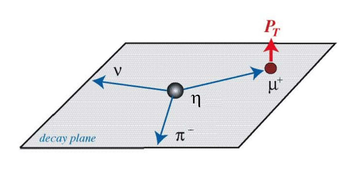
Figure 15: Transverse muon polarization P_T in Dalitz (left) and semileptonic (right) $\eta$ decays at rest.

The Standard Model prediction for $P_{T}$ is extremely small, arising only from higher-order loop contributions Bigi and Sanda (1999). As an example, these have been computed in the context of Kaon decays Zhitnitskii (1980); Efrosinin et al. (2000), finding them at the $10^{-5}$level — similar results should apply to $\eta\to\pi^{-}\mu^{+}\nu$ decays. More complex models involving New Physics such as multi-Higgs doublet models, leptoquark models or supersymmetric models with R-parity breaking or s-quark mixing predict much larger values for $P_{T}$ ranging from $10^{-4}$ to $10^{-2}$ Garisto and Kane (1991); Wu and Ng (1997). As an aside note, the $\eta\rightarrow\pi\mu\nu_{\mu}$ process has not been observed yet.

In Dalitz decays, $\eta\to\gamma\ell^{+}\ell^{-}$, the leading order QED and weak contributions do not contribute to such an asymmetry Sanchez-Puertas (2019), such that any positive observation at REDTOP would correspond to physics BSM. Likewise, in $\eta\to\pi^{0}\mu^{+}\mu^{-}$, no contribution to such an asymmetry was found in Escribano et al. (2022a), such that any positive finding would point to physics BSM.

In conclusions, any observation of a transverse muon polarization in the 3-body decays of $\eta/\eta^{\prime}$ mesons is an unambiguous indication of $CPT$ violation and physics BSM.

V.3 Polarization in Dalitz decays

By contrast to the $\eta\to\mu^{+}\mu^{-}$ case, Dalitz decays provide more opportunities regarding muon polarization observables. On the one hand, compared to parity-violating asymmetries in $\eta\to\mu^{+}\mu^{-}$ decays (which are necessarily $CP$ odd), parity-violating asymmetries in Dalitz decays are potentially more sensitive to $CP$-even physics. This is related to the fact that $CP$-odd contributions require unitary phases on the basis of the $CPT$ theorem, which are small in Dalitz decays. As an example, $CP$-even weak interactions do contribute to $P_{L}$ due to $Z$-boson exchange Bernabeu et al. (1998). These are however small (note the typical suppression factor $G_{F}m_{\eta}^{2}/\alpha\sim 10^{-5}$ with respect to the QED contribution). In particular, a contribution of $6\times 10^{-7}$ was found in Sanchez-Puertas (2019) for $A_{L}$ (see Eq. (75)), that is beyond REDTOP statistics. Hence any positive finding would point to BSM physics. On the other hand, further asymmetries can be studied, see for instance the transverse plane asymmetry above or those defined in Ref. Sanchez-Puertas (2019).

V.4 Polarization in $\eta\to\pi^{0}\mu^{+}\mu^{-}$ decays

Similar to Dalitz decays, the richer dynamics of this process allows for further opportunities as compared to the $\eta\to\mu^{+}\mu^{-}$ case (note for instance the transverse plane asymmetry among others). However, by contrast to the Dalitz decays, and in the context of parity violating asymmetries, $CP$-violating contributions arise at lower dimension than $CP$-even ones, see Ref. Escribano et al. (2022a). Further, the SM QED amplitude features a large unitary phase due to the intermediate 2-photon exchange, potentially enhancing the sensitivity to $CP$-odd scenarios over $CP$-even ones. As a final note, the SM $P$-odd, $CP$-even contribution would arise through $\gamma Z$ box diagrams, that are highly suppressed for REDTOP statistics. Hence any positive finding would clearly point to BSM physics.

VI The REDTOP experiment

The most efficient way to produce $\eta/\eta^{\prime}$ mesons is from nuclear scattering of a proton beam onto a nuclear target. Above E${}_{kin}\approx 1.2$ GeV several intra-nuclear baryonic resonances are created, whose decay produce an $\eta$-meson. The $\eta$ production cross section increases rapidly above threshold (see left plot in Figure 16), and the desired yield can be achieve with a beam energies below 2 GeV.

VI.1 Hadro-production of $\eta$ mesons

An important aspect in properly designing the REDTOP detector and the accelerator complex, is the estimation of the $\eta$-meson production parameters. The most abundant hadro-production mode of $\eta$/$\eta^{\prime}$-mesons occur via the formation and decay of intranuclear baryonic resonances ($\varDelta$’s, N(1440), N(1535), etc.) in nucleon-nucleon collisions. The cross section for such processes is about seven times larger in $p-n$ collisions than $p-p$ ones. Therefore the nuclear target should have a large neutron to proton ratio. A target with low-Z minimizes the formation of nuclear fragmentation products, and helps to reduce the particle multiplicity of the final state.

The beam energy should be above the threshold for $\eta$/$\eta^{\prime}$ production of 1.2 GeV and below the kaon production threshold of 3.3 GeV, since the decay of kaons could mimic the decay of a new long-lived particle. Extensive studies have been conducted with the GenieHad Gatto (2012) event-generator framework using multiple beam and target parameters. Figure 16 shows GenieHad predictions for beam energy dependence of the total $p+Li$ inelastic cross section (left) and the probability to produce an $\eta$ (right). Above threshold, the total $\eta$/$\eta^{\prime}$ production cross section increases approximately linearly with beam energy. One consequence of the resonant production mechanism is that the momentum of the $\eta$/$\eta^{\prime}$ mesons in the lab frame is only sligthly dependent from the beam energy, in a interval spanning several hundred MeV above threshold. Such studies indicate that a proton beam with E${}_{kin}\approx 1.8-1.9$ GeV impinging on a thin, low-Z, high-$\nicefrac{{A}}{{Z}}$ material like Beryllium or Lithium is an optimal choice for the experimental program.

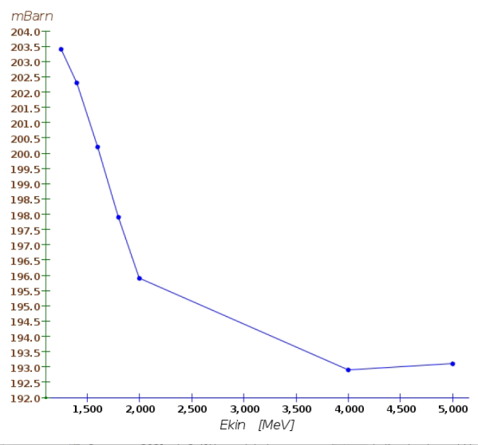
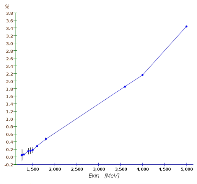
Figure 16: Predictions of $p+Li$ cross sections versus beam energy from the GenieHad Gatto (2012) model with Urqmd +Abla07 scattering models using the Tripathi parametrization for the inelastic cross section. The left panel shows the inelastic cross section while the right panel shows the percentage of such collisions that produce an $\eta$ meson.

Unfortunately, no experimental data on the $p-Li$ inelastic cross section nor $\eta$/$\eta^{\prime}$ production exist in this energy range. Furthermore, the abundance of intra-nuclear resonances complicate the formulation of theoretical models as they require non-trivial treatment within a non-perturbative approach. To minimize the uncertainty in calculating the $\eta$/$\eta^{\prime}$ production cross section, we used several models in GenieHad to calculate the cross section and compared few nuclear transport models to describe the evolution of proton-nucleus collisions. The total $p-target$ inelastic cross section has been calculated for protons with $E_{kin}$= 1.8 GeV by averaging seven different models and a detailed description of the target including, besides the lithium core, thin protective epoxy and copper layers. The results of these calculations are summarized in Tab. 7.

Model	p-Li cross section	p-Li	p-Target
	[cm${}^{-2}]$	interaction prob.	interaction prob.
Wellisch & Axen	$2.01\times 10^{-25}$	$0.710\%$	$0.719\%$
Tripathi Light	$1.96\times 10^{-25}$	$0.693\%$	$0.702\%$
Incl++	$1.60\times 10^{-25}$	$0.567\%$	$0.574\%$
Sihver et. al	$1.51\times 10^{-25}$	$0.535\%$	$0.543\%$
Barashenkov	$1.73\times 10^{-25}$	$0.612\%$	$0.620\%$
Shen et. al	$2.0\times 10^{-25}$	$0.707\%$	$0.715\%$
Kox et. al	$2.98\times 10^{-25}$	$1.06\%$	$1.07\%$
$Average$	$1.98\pm 0.48\times 10^{-25}$	$0.70\pm 0.17\%$	$0.71\pm 0.17\%$

Table 7: Estimate of inelastic cross section and interaction probability for protons $E_{kin}$= 1.8 GeV on REDTOP targets using different models in GenieHad Gatto (2012). The error indicates the standard deviation.

In order the estimate the $\eta$ yield at REDTOP, the outcome of four $GenieHad$ hadronic generator models was examined. The $\eta$ production probability in inelastic $p+Li$ collisions at 1.8 GeV is summarized in in Tab. 8.

Nuclear collision model	p+Li
	$\eta$ yield
Urqmd Bleicher et al. (1999)	$0.49\%$
Incl++ v6.2 Hirtz et al. (2020)	$1.48\%$
Gibuu v2019 Buss et al. (2012)	$0.74\%$
PHSD v 4.0 Ehehalt and Cassing (1996)	$0.67\%$
Jam v1.9 Nara, Yasushi (2019)	$0.26\%$
$Average$	$(0.73\pm 0.46)\%$

Table 8: Estimate of $\eta$ production probability in inelastic collisions at $E_{kin}$= 1.8 GeV on REDTOP targets using different models in GenieHad Gatto (2012). The error indicates the standard deviation.

The average valued is: $Prob(p+Li\rightarrow\eta\,X)\approx(0.73\pm 0.46)\%$. Assuming $10^{18}$ POT, the yields of $\eta$/ $\eta^{\prime}$ and of inelastic proton interactions are summarizes in Table 9. .

	Expected yield for $E_{kin}$=1.8 GeV
$N_{\eta}$	$5.1\times 10^{13}$
$N_{\eta^{\prime}}$	0
$N_{ni}$	$7\times 10^{15}$

   Expected yield $E_{kin}$=3.6 GeV $N_{\eta}$ $1.8\times 10^{14}$ $N_{\eta^{\prime}}$ $2.4\times 10^{11}$ $N_{ni}$ $9.7\times 10^{15}$

Table 9: Expected $\eta$ and $\eta^{\prime}$ yield at REDTOP for $10^{18}$ POT (see Sec. VII.1 for details on the estimation method)

A similar analysis with Urqmd indicates that the inelastic proton scattering probability on REDTOP target with an $E_{kin}$=3.6 GeV is 0.68% (a factor $\sim 1.4\times$ than at 1.8 GeV. On the other side, the fraction of $\eta^{\prime}$ mesons in such events is $2.5\times 10^{-5}$. The corresponding $\eta^{\prime}$ yield is summarized in Table 9.

VI.2 Beam and target requirements

Following the discussion in Sec. VI.1, the beam energy chosen for the $\eta$ run of REDTOP is 1.8 GeV, where the neutral kaon production probability for $p+Li$ collisions is about $1.8\times 10^{-4}$. It was also noted that the higher$\nicefrac{{A}}{{Z}}$of the Li, compared to the rest of low-Z nuclei, makes it an ideal material for REDTOP target systems. For example, the multiplicity of primary neutrons produced by a Nb target increases more than 20% wrt a Be target, while the increase of primary protons is almost 90% (from GenieHad simulations). Fig. 17 summarizes the multiplicity of pions, protons and neutrons for QCD events non containing and $\eta$ or $\eta^{\prime}$ meson (GenieHad simulation with Urqmd +Abla07 scattering models). An important requirement for REDTOP is minimizing the rescattering of the $\eta$ decay products inside the target This is achieved by splitting the latter in multiple thinner foils. That would, on one side, improve the measurement of the z-coordinate of the $\eta$ production vertex, and, on the other side, it minimizes the multiple scattering affecting the $\eta$ decay products when they escape from the target. By using 10 foils, spaced 10 cm apart, one would provide the necessary total material budget for the required luminosity, while the pile-up due to multiple beam interactions within the same trigger could be easily reduced with vertexing techniques. A similar study for the $\eta^{\prime}$ case yields an optimal range for E_kin of about 3.5-4 GeV.

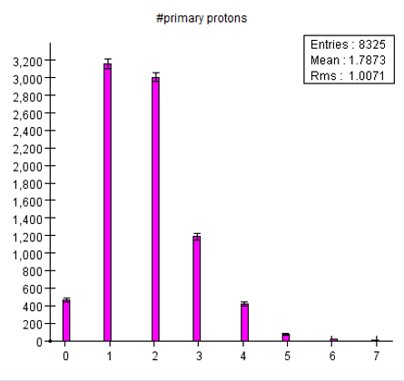
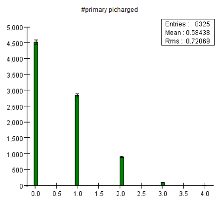
Figure 17: Multiplicity of pions, protons and neutrons for p-Li scattering at 1.8 GeV for events without a $\eta$ or $\eta^{\prime}$ meson (GenieHad simulation with Urqmd +Abla07 scattering models).

In conclusion, a CW proton beam delivering $1\times 10{}^{11}$POT/sec would generate a rate of inelastic interaction of about 1 GHz and a $\eta$-meson yield of $5.1\times 10{}^{6}\eta/sec$, corresponding to $5.1\times 10{}^{13}\eta/yr.$ The beam power corresponding to the above parameters is approx. 30 W, of which 1% (or 300 mW) is absorbed in the target systems. Each of the 10 foils will have to dissipate about 30 mW, which is easily achievable by convection of the accumulated heat through the foil holders. These estimate roughly double for the beam required when running at the $\eta^{\prime}$.

VI.3 Detector requirements

The $\eta$ mesons generated with the above beam parameters are almost at rest in the lab frame, receiving only a small boost in the direction of the incoming beam (see Fig. 18). This is a consequence of their production mechanism as they are the decay products of an intranuclear resonance in the target material. Studies performed with GenieHad have indicated that the $\eta-$spectrum is almost independent from the beam energies in the [1.46-2.1] GeV range. Consequently, an hermetic detector covering the entire solid angle, is one of the requirements for REDTOP.

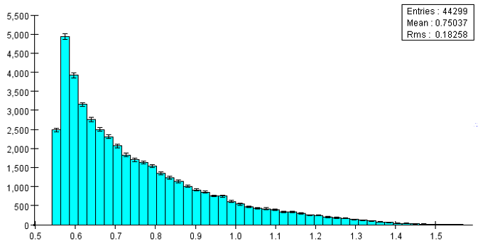
Figure 18: Total energy of $\eta$ mesons from a $E_{kin}$=1.8 GeV proton beam scattered on REDTOP targets (GenieHad simulation).

A correct identification of the final state particles is, also, of paramount importance for an experiment exploring rare processes. On one side, the vast majority of the processes listed in Fig. 1 have two leptons at at least one photon in the final state. On the other side, the QCD background, which has a production rate two order of magnitudes larger, is populated almost invariably by protons, neutrons, slow pions and nuclear remnants. These are relatively slow particles, as shown in Fig. 18 for the case of protons and pions. Furthermore, neutrons impinging onto the calorimeter would easily be mistaken as photons if a proper particle identification (PID) is not in place. Finally, the identification of$e^{+}e^{-}$ pairs from photons converting in the material upstream the central tracker will help to reject the large background originating from QCD production of $\pi^{0}$ particles. The detector is inserted in a solenoidal magnetic field which bends the charged particles for proper $P_{t}$ and electric charge measurement.

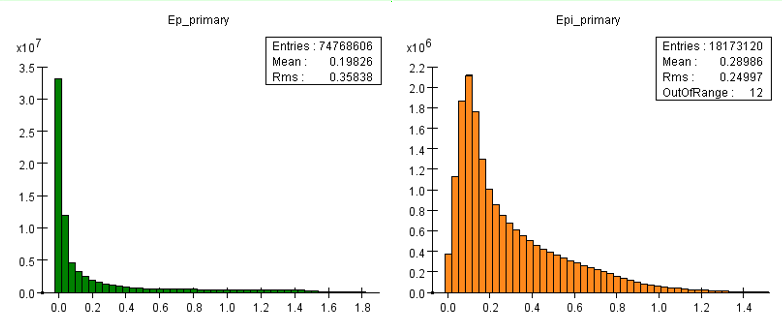
Figure 19: Momentum of protons (left) and charged pions(right) from inelastic scattering of a $E_{kin}$=1.8 GeV proton on REDTOP targets (GenieHad simulation).

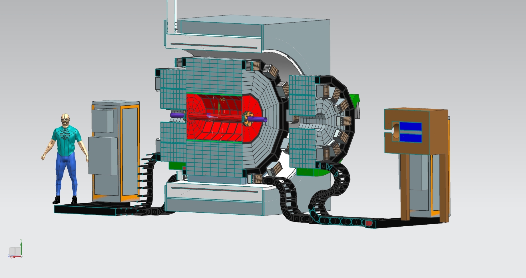
Figure 20: Cross section of REDTOP detector

VI.4 The REDTOP detector

A baseline detector layout has been defined for preliminary studies of sensitivity to a broad range of BSM physics processes. Cost optimization is deferred to at a later stage of the project. The individual components of REDTOP detector are briefly summarized below.

VI.4.1 The vertex detector

The vertex detector has four main tasks: a) identifying events with a detached secondary vertex. b) contributing to the reconstruction of charged tracks originating in the target; c) rejecting photons converting in the target; d) reconstructing track with very low transverse momentum. Two detector technology options are currently being investigated for the vertex detector: a wafer-scale silicon sensor and a thin scintillating fiber tracker.

The most important challenges for REDTOP vertex detector are related to the material budget and to its proximity to the interaction region. Keeping the material budget as low as possible is a necessary requirement to reduce the multiple scattering, which would, otherwise, compromise the momentum resolution and increase the background from photon conversion. The main requirements for the vertex detector, derived from the sensitivity studies to several benchmark processes (cf. Sec. VIII and XIII) are listed below:

• A spatial resolution near the IP better than 20 μm;

• Material budget: $\sim$0.03% $X_{0}$/layer;

• Radiation hard up to of $\sim 5\times 10^{6}$/cm²/s “1-MeV equivalent neutron fluence” (or $\sim 5\times 10^{13}$/cm² integrated over 1 year (see, also, Sec. XIX);

• Coverage: $\sim$96% of full solid angle.

Vertex detector option I – Fiber tracker

A fiber tracker, with an identical technology as implemented for the LHCb upgrade(Kirn et al., 2017), is located around the beam pipe, at a radius r $\approx$5 cm around the z-axis. Three superlayers are stacked together, interspaced with structural foam 1 cm thick, providing mechanical stability to the subdetector. Each superlayer consists of a mat with 5 layers of scintillating fibers, with a diameter of 250 $\mu m$. The space resolution of each superlayer is $\sim 70\mu m$, as measured by LHCb at a test beam. The fiber tracker serves two main purposes: a) it provides a vertex measurement for the reconstructed event, and b) it identifies photons converting into $e^{+}e^{-}$ pairs inside the OTPC (typically, in the inner wall of the chamber or in the aerogel). The determination of the primary vertex of the event identifies the foil where the inelastic interaction occurred and it provides the position of the $\eta$-mesons.

Vertex detector option II – Wafer-scale silicon sensor

This option is based on the current R&D performed by Alice collaboration for their ITS3 detector. It consists of three-layer of flexible Silicon Genesis: 20 micron thick wafer, with CMOS sensors. The wafer-scale sensors are 900 mm long, fabricated using stitching. A total of six such sensors is needed to cover the innermost region of REDTOP. Key benefits of this option are: a) a material budget corresponding to mere 0.02-0.04% $X_{0}$; b) an homogeneous material distribution, resulting in an almost-negligible systematic error from the material; c) a 3-dimensional hit information. A picture of the ITS detector proposed by Alice is shown in Fig. 21.

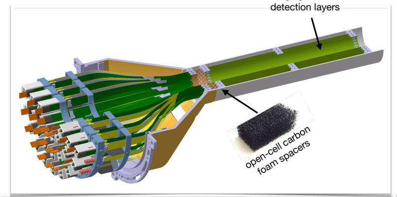
Figure 21: Schematics of Alice proposed ITS3 tracker

VI.4.2 The central tracker

Requirements for central tracking

The two largest challenges for REDTOP tracking are related to the relatively low momentum of the particles that have to be reconstructed. These are: a) a very low material budget to reduce the multiple scattering as much as possible, and b) a time resolution sufficient to contribute to the TOF systems for identifying the particles. In other words, the central tracker needs to be able to reconstruct charged tracks in four dimensions. The main requirements for the central tracker, derived from the sensitivity studies to several benchmark processes (cf.  Sec. VIII and XIII) are listed below:

• Momentum resolution: $\sigma_{P_{T}}/P_{T}^{2}\sim 2\times 10^{-3}$ GeV^-1at P_T=1 GeV;

• Material budget: $\sim$0.1% $X_{0}$/layer;

• Time resolutions: $<30psec$;

• Coverage: $\sim$96% of full solid angle

Two technologies have been considere for REDTOP central tracker: a) low-mass LGAD, and b) an Optical TPC.

Central Tracker option #1: low-mass LGAD tracker

Recent advancements in silicon particle sensors enable precise timing of MIP signals, though a sensor design called Low Gain Avalance Detectors (LGAD). Compared to the p-n junction of a standard semiconductor, the LGAD adds a highly-doped layer. When depleted, this results in a stronger electric field locally, causing electrons to avalanche in that region. The better signal-to-noise improves the timing resolution of the detector.

Current LGAD sensor technology can meet the timing performance requirements of REDTOP. The ATLAS and CMS collaborations plan dedicated layers of LGAD detectors for the forward regions to measure the time of arrival of particles, with a primary motivation being the rejection of tracks from pileup events ATLAS Collaboration (2020); CMS Collaboration (2019). Radiation hardness is a primary consideration for these detectors, since they must tolerate fluences well over $10^{15}$ n${}_{\text{eq}}$/cm². Both detectors plan a spatial granularity of $1.3\times 1.3\ \mu$m².

The most recent improvements have been in the spatial segmentation of the detectors. Timing resolution of 30 ps and spatial resolution better than 10 $\mu$m has been observed in testbeam measurements of AC-coupled LGAD sensors Heller et al. (2022). LGADs separated by a physical trench (“Trench-isolated” or “TI-LGAD”) are also a promising direction, with TCT tests showing timing performance on the order of 5 ps prior to irradiation Senger et al. (2022).

The majority of the material in the ATLAS and CMS timing layers is cooling and mechanical support, with the sensor and readout chip are typically only comprising a few percent of the total. To meet the material budget of REDTOP, only passive cooling can be used. Carbon-fiber support structures similar to those planned for the HL-LHC upgrade of the pixel detector are strong, lightweight, and have good thermal conductivity. The system, particularly the readout electronics, must be designed to minimize the heat output.

Central Tracker option #2: The Optical TPC

Protons and slow pions account for the largest charged background at REDTOP. In average 0.6 charged pions and 1.8 protons are produced every nsec in the target systems by the $E_{kin}$=1.8 GeV proton beam.

Figure 22: Charged pions (left) and proton (right) multiplicity from inelastic scattering of a $E_{kin}$=1.8 GeV proton on REDTOP targets (GenieHad simulation).

A charged track detector mostly blind to them is required in order to identify more rare decays. These particles have a consistently low value of $\beta.$ Consequently, the threshold characteristic of the Cerenkov effect could be exploited to build a detector insensitive to this hind of background.

An Optical TPC(Frisch, 2014; Oberta and Frisch, 2015) (OTPC) (the red dodecagon in FIG. 20) measures the transverse momentum and the $\beta$ of fast particles ( of electrons, muons and fast pions). It is a vessel filled with gas ($CH_{4}$) with the inner wall covered by an aerogel radiator with a thickness of $\simeq$3 cm. The external walls of the chamber are instrumented with optical photo-sensors (LAPPD or sipm’s) with a pixel size of few $mm^{2}$. When an electron or a positron with a $\beta$ above the Cerenkov threshold of $CH_{4}$ traverses the gas, it bends in the solenoidal magnetic field while also radiating photons. The shape of the latter, being collected by the photo-sensors covering the outer walls of the device, has a specific pattern which provides the $P_{t}$ of the particle. Position and direction of the particle are obtained by combining the pattern of the light ring, radiated from the aerogel, with the information of the impinging point on the photo-sensors.

Slower particles like muons and pions, typically with $\beta$ below the Cerenkov threshold in the gas, produce a characteristic photon ring when they cross the aerogel. The latter is detected from the OTPC photo-sensors and reconstructed, providing a measurement of the kinematic parameters of the particle. Protons and pions from QCD scattering are consistently below detection sensitivity of the OTPC and do not constitute a sizable background for the experiment. The magnetic field (0.6 T) also provides the magnetic bottling preventing these very slow particles particles from reaching the calorimeter with elevated rates.

Material budget for the baseline tracking layout

The geometry of the baseline detector, consisting of the fiber tracker, the LGAD central tracker, the Threshold Cerenkov Radiator, and ADRIANO2 calorimeter, has been implemented in the software framework and used to perform all physics and detector studies presented in the second part of this paper. An estimate of the material budget for the tracking region of the detector (r<50 cm) is shown in Fig. 23 as function of the transverse radius. The plots indicate that the beam pipe contributes with $\simeq$0.2%  of $X/X_{o}$, the fiber tracker with $\simeq$ 0.3%  per layer, while the central tracker contribution is $\simeq$ 0.2% per layer.

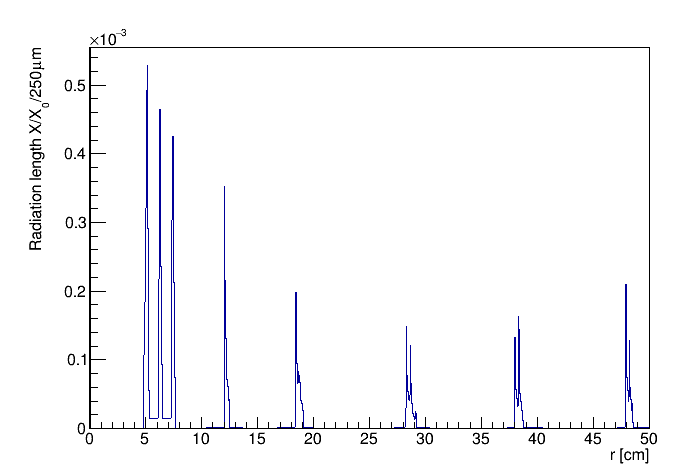
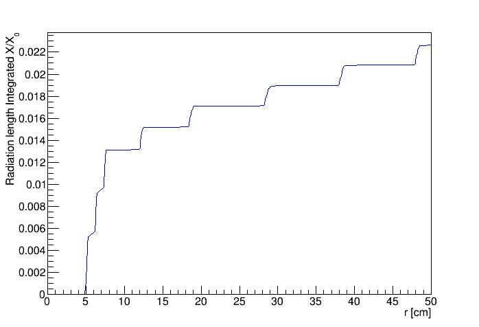
Figure 23: Plot of $X/X_{o}$ as a function of the transverse radius for the baseline tracking system of REDTOP. The calculation is performed in radial steps of 250 $\mu m$ (left). The integrated material budget is shown in the right plot.

VI.4.3 Electromagnetic and hadronic calorimeter: ADRIANO2

Requirements for calorimetry

REDTOP calorimetry presents several challenging requirements since, besides measuring the energy and he time of arrival of an impinging particle, it also participates to all levels of triggers. The latter implicates that it needs to provide to the trigger system pre-processed information on a very short time scale.The required performance has been assessed on the base of the sensitivity to several benchmark processes. A full discussion of the latter has been carried in Secs. VIII, XIII and XIV. The main requirements for REDTOP calorimeter are:

• Energy resolution: $\sigma_{E}/E=3\%/\sqrt{E}$

• Particle Identification (PID) with separation efficiency between electromagnetic and hadronic particles higher than 99%;

• Time resolution: $<80psec$ in a single cell with energy deposit > 7 pe;

• Detector response: within $\leavevmode\nobreak\ 100nsec$;

• Reconstruction efficiency: >50% for E>20 MeV and >90% for E>80 MeV.

The first requirement is fulfills the need to identify $\pi^{0}$ mesons produced in the target from the primary interaction, since their decay products make one of the largest combinatoric background. This could be accomplished by fully reconstructing the decay of $\pi^{0}$ into $\gamma\gamma$ and $\gamma e^{+}e^{-}$, which can be achieved with a sufficiently good energy resolution. Furthermore, several decays of the $\eta/\eta^{\prime}$ mesons contain $\gamma^{\prime}s$ or $\pi^{0}$’s in their final state. In those cases, an higher energy resolution will allow a more efficient reconstruction of events associated to $\eta/\eta^{\prime}$ decays en, consequently, a better $signal/background$ ratio.

Particle identification is also important to reduce the hadronic background. As discussed in details in Sec. VI.5, a fast PID algorithm has to be implemented already in the Level-0 trigger, to reduce the number of non-$\eta/\eta^{\prime}$ events to a more manageable level. As discussed below, a fast particle identification can be implemented using dual-readout techniques. The requirement on time resolution is also affects the PID, since baryonic particles (which constitute the largest fraction of background particles generated in the primary interaction), have a much slower Time-of-Flight compared to the $\eta/\eta^{\prime}$ decay products. A fast detector response is an essential requirement, considering also that the total expected event rate in the calorimeter is of order of 0.7 GHz. Assuming a pipeline with a depth of fifty , the event needs to be processed by the Level-0 trigger in less than 100 nsec.

The technology chosen for filfilling the above requirements is a special implementation of dual-readout calorimetry called: $ADRIANO2$, briefly described below. The calorimeter is divided into two sections. The innermost section (about 40 cm in depth, or $\sim 17\nicefrac{{X}}{{X_{0}}}$) is a high-granularity, integrally active dual-readout calorimeter, made of alternated tiles of lead-glass and scintillating plastics, optically separated and read-out individually.

Its main tasks are to reconstruct electromagnetic showers and to measure the energy of photons and electrons. The outermost section has the same layout of the innermost section, but it includes plates of passive material sandwiched with the active layers. The passive material reduces the nuclear interaction length so that hadronic showers will be fully contained in the overall depth of the calorimeter (about 80 cm). Both sections have dual-readout capabilities and participate in the PID and TOF systems.

The dual-readout technique

Dual-readout (DR) calorimetry(DRE, 2000; Gatto, 2015a) is a relatively novel technique aiming at achieving energy compensation in hadronic showers produced in high energy experiments. One particular implementation: ADRIANO, where both readout components are integrally active, has been developed in recent years by T1015 Collaboration(Gatto, 2015b, c) for applications in future lepton colliders or high intensity experiments requiring low granularity. ADRIANO building block is an integrally active log made by sandwiching lead glass and scintillating plates, optically separated and with independent readouts. The Cerenkov and scintillating lights are captured by wavelength shifting fibers (WLS) coupled to light sensors.

One of the advantages of ADRIANO is that, with a proper layout, the dual-readout method can be used also for electromagnetic calorimeters as a way to identify a particle by comparing the response of the two components. The particle separation with a dual-readout calorimeter is illustrated in Fig. 24 for particles of different species and same energy (100 MeV). The separation between photons and neutrons, is better than 4$\sigma$, and it far exceeds the required limit of 99% .

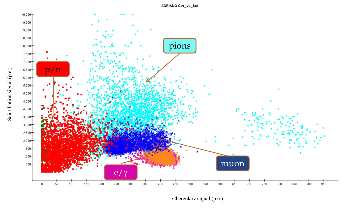
Figure 24: Plot of S vs Č signals for several 100 MeV particles in ADRIANO (ilcroot simulation)

REDTOP requires a finer granularity than it could be achieved with the log based, ADRIANO technique. A higher granularity implementation is, therefore, being considered: ADRIANO2, where the lead-glass and the scintillating strips are replaced by small tiles with direct SiPM readout (Blazey et al., 2009; Abu-Ajamieh et al., 2011; Malla, 2019). ADRIANO2 is a relatively compact calorimeter, combining Particle Flow reconstruction (PF) (segmentation in space and potentially in time) and DR (multiple readout). See reference  Sefkow et al. (2016) and references therein for details on the particle Flow technique. The compound benefits of either algorithms have a great potential interest for future applications besides REDTOPGroup (2020). Recent studies by T1604 Collaboration indicate that the small size of the lead glass tiles and the prompt nature of the Cerenkov light, when captured by a fast SiPM, meet the timing requirement for the calorimeter discussed above.

The ADRIANO2 Calorimeter

ADRIANO2 is fabricated with alternate tiles of lead-glass and scintillating plastic, optically separated and red-out individually. For an optimal collection of the Cerenkov light, the lead-glass tiles (size = 1$\times$3$\times$3 cm³) are coated with either a diffuse or reflecting metal for example Ag, Al, Mo, W, etc. Various thin film deposition methods such as sputtering, electroplating, evaporation, chemical vapor deposition (CVD) and atomic layer deposition (ALD) are currently being explored. Among the various thin film coating methods, ALD method can offer outstanding control of thickness and excellent film uniformity. As self-limiting reactions between gaseous precursor and a solid surface involved in ALD process, therefore, this method can produce clean thin films in an atomic layer-by-layer way with precise control over layer thickness and composition. This feature allows precise coatings to be applied on all exposed surfaces of complex substrates such as fibers, woven, nanotubes, aerogels, mesoporous, nanoporous, membranes and solid geometries. For applications where highly conformal deposition of thin films is required, the acceptable control can only be achieved with ALD methods. ALD can also be scaled to coat large batches of 3D parts simultaneously. Considering the lead-glass cube 3D form factor, here we have explored the ALD material coating method, which seems to be very promising.

Recent tests with 100 nm thick W and Mo coating by optimized ALD method using the combination of WF6-Si2H6 or MoF6 –Si2H6 precursors and a 10 nm thick composite barrier Mane and Elam (2018). The quality of the deposited W or Mo layer were analyzed by x-ray photoelectron spectroscopy (XPS) for composition and four probe measurements for electrical conductivity. The photograph of lead-glass cube before and after ALD is shown in Fig. 25.

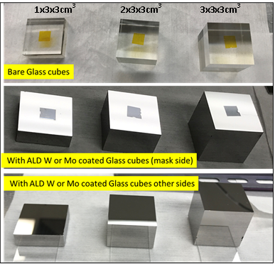
Figure 25: Top row different size bare lead-glass cubes with kapton tape mask placed on one of the side. Middle row lead-glass cubes after W or Mo ALD and kapton masked removed. Bottom row non-masked sides lead-glass cubes coated with W or Mo ALD.

Performance of these W and Mo ALD coated cubes were tested at Fermilab and have shown, so far, excellent results compare to other coating methods e.g. sputtering, spray paint, evaporation which were evaluated.

Readout electronics

One In order to fulfill the constraints above, stingent requirements need to be placed on the Front-End Electronics (FEE).

One possible alternative to the analogue sipm readout is based on the novel technique of $SinglePhotonCountingDetector$ (SPAD) which reperesent a particular implementation of Digital Photon Counters (DPC), where the readout electronics is incorporated in the photosensor. SPAD array in CMOS technologies may offer the following benefits to fast calorimeters:

• incorporation of complex functions in the same substrate (e.g. SPAD masking, counting, TDCs);

• optimization of the design of the front-end electronics to preserve signal integrity (especially useful for timing)

• easier assembly due to the monolithic structure of the sensor;

• significantly reduced temperature sensitivity by at least one-order-of magnitude

• reduced afterpulsing & crosstalk

• better linearityand intrinsic timing resolution due to integrated TDCs ($\simeq$ factor 5)

• no analog electronics, no ADCs, no ASICs

• power consumption, which is especially important in calorimeters like the one proposed, where the readout-electronic is embedded inside the volume of the detector and excess heat needs to be removed.

VI.4.4 The Threshold Cerenkov Radiator (TCR)

A thin Cerenkov radiator is inserted between the Central Tracker and the calorimeter. The detector has two main purposes: a) the detection of particles above the Cerenkov threshold provided by quartz; b) the measure of the TOF of such particles. The information from the $TCR$ is also used in the Level-0 trigger to reduce the contamination of the signal events from slow baryonic particles. Finally, the $TCR$ complements the energy measurements of the calorimeter as it operate as a lower density pre-shower.

The requirements for the $TCR$ are :

• Time resolutions: $<50psec$;

• Detector response: within $\leavevmode\nobreak\ 100nsec$

• High-granularity to reduce overlapping showers.

The baseline layout of the $TCR$ consists of small tiles made of borosilicate JGS1 glass, which is transparent to UV light above $\simeq$200 nm. The latter is abundantly produced by the Cerenkov effect from all particles above threshold. The momentum threshold for the various particle species is summarized in Table 10.

PID	Momentum threshold
	[MeV/c]
electron	$0.4$
muon	$100$
pion	$130$
proton	$870$

Table 10: Cerenkov threshold of $TCR$ detector.

The dimension of the tiles is $3\times 3\times 2\>cm^{3}$, namely, they have the same footprint of ADRIANO2 tiles. The Cerenkov light is read-out by a NUV-SiPM optically coupled to each unit. The analog information from the $TCR$ is also used in the reconstruction of showers in the ADRIANO2 calorimeter.

VI.4.5 The Timing Layer ($TL$, optional)

A further improvement to the PID systems could come from the TOF system when the requirement on timing resolution of the $TCR$ is lowered to 30 psec or less. Preliminary studies performed by T1604 collaboration indicate that a such a resolution could be beyond the limits of the technology adopted for the TCR. An optional AC-LGAD Timing Layer ($TL$), based on the design planned for experiments at the Electron Ion Collider (EIC), would be able to reach the desired goal. The proposed layout for REDTOP would employ the $TCR$ as supporting structure, contributing to a small fraction of the material budget of the $TL$, with negligible impact on the performance of the ADRIANO2 calorimeter.

A joint effort to develop such a TL for REDTOP and EIC experiments can benefit both experiments, which have similar requirements on the timing resolution and material budget. For example, a cylindrical TL with a radius of about 50 cm is envisioned for EIC experiments that require a single hit timing resolution better than 30 ps, and a material budget per layer less than 1%. Such a design could be realized by long-strip AC-LGAD sensors with thin sensor active volume, and low-power and low-jitter frontend readout ASICs, which are currently being developed by the eRD112 collaboration for EIC et al. (eRD112).

VI.4.6 The Muon Polarimeter (MuPol, optional)

The construction of a dedicated muon polarimeter is being consideration for REDTOP in case the ADRIANO2 performance would not be adequate to for polarization measurements. The muon polarimeter has the task of stopping the muons from the $\eta/\eta^{\prime}$ decays and detect the direction of the electron or positron. The design of such detector is based on the proposal of the TREK experimentKohl (2010) at J-PARC. The proposed technology implements the concept of an active polarimeter, which attain higher detector acceptance and higher sensitivity compared to a conventional passive polarimeter. The main advantage of an active technique is that the muon decay vertices will be determined event-by-event, which make the polarization measurement free from the systematic error associated with the uncertainties of the muon stopping distribution.

The polarimeter would consist of two parts: a) a set of passive plates, where the muon will either stop or decay in flight, interspersed with b) tracking chambers where the electron or positron would be detected. A large muon stopping efficiency in relatively small volume requires higher average material density. On the other side, a clean detection of positrons without interactions such as bremsstrahlung or annihilation in flight requires a material with lower average density and the use of low mass elements. Aluminum and magnesium (or their alloys) are good candidates as they are also know for their property of not affecting the original polarization of the muon. An integrated thickness of $\sim 66mm$ of aluminum will have a stopping power of $\sim 85\%,$which is sufficient to perform excellent polarization measurements with the expected event statistics foreseen at REDTOP.

The elector/positron tracking chambers will be located between the stopping plates. Two technologies are being considered: a) a gaseous wire chamber, and b) a fiber tracker. The former has the advantage of being low cost in terms of construction and readout-electronics. The latter has the advantage of simplicity and low maintenance. Square scintillating fibers with sides as large as 2 mm are commercially available with short lead times and, when glued to the stopping plates, will contribute to the mechanical robustness of the detector. In both cases, the coordinate along the wire or fiber is determined by charge or light division at both ends.

The electron or positron energy will be determined using both the range in the stopper material and the trajectory curvature in the field. The tracking is done by taking into account energy loss through each plate. In a design using aluminum plates, the total material thickness in the radial direction is $\sim$13 $g/cm^{2}$ to be compared with the range of electron or positron of 5 $g/cm^{2}$ for 10 MeV and 15 $g/cm^{2}$ for 25 MeV.

The $MuPol$ will be positioned inside the calorimeter at a depth of approximately 20 radiation lengths, to avoid any degradation of the energy measurement in ADRIANO2. The design allow to perform a measurement of the electron or positron energy as well as its emission angle, by using the outer section of ADRIANO2, with a significant increase in the analyzing power of the polarimeter, and, consequently, in a higher sensitivity. Furthermore the materials in front of the MuPol, essentially lead glass and scintillating plastics, are amorphous and, unlike the crystals used in most of the high resolution electromagnetic calorimeters, do not change or degrade the original polarization of the muon. The latter will be slow down before entering the passive plates of the $MuPol$, with higher probability of being stopped in the passive metal plates.

Although the stopping material alone is not thick enough to stop an electron from a muon near the surface, additional range stacks besides the stopper are useful to discriminate lower energy electrons with a negative asymmetry. With the magnetic field foreseen for REDTOP (see next section), the bending radius for a 25 MeV electron is 650 cm. A moderate position resolution of several 100 $\mu$m will be able to determine the energy of positron with a 10 cm long track with an accuracy of $\sim$40%.

VI.4.7 Superconducting solenoid

A 0.6 T solenoidal magnetic field is required to measure the $P_{t}$ of the particles with $\beta\approx 1$. The field will also magnetically bottle the very low momentum particles, preventing them from reaching the calorimeter. The solenoid built for the, now dismantled, Finuda experiments (Bertani et al., 1999) matches all operational and dimensional parameter required for REDTOP. It also fits through the hatch that connects the AP50 hall (for the Fermilab running option, cf. Appendix XVII) and it can be transported on rails to its final location. The same magnet could be accomodated even more easily in the C4 beamline, for a possible run at BNL.

VI.5 The event trigger systems

The goal of producing $5.2\times 10^{13}$ $\eta$ mesons per year, ( $5.2\times 10^{6}$ $\eta$/s, assuming $10^{7}$ seconds of useful running time), requires about $7\times 10^{8}$ $p$-Li inelastic collisions per second (cf. Table 8). This rate can be achieved with a proton beam intensity of $10^{11}$ $p$/s and a Li target of $2\times 10^{-2}$ collision lengths ($\approx$ 7.7 mm total thickness), possibly subdivided into a number of thinner layers. Taking into account the total p-Li inelastic collision rate, we estimate that the total rate of events reaching the detector is $\sim 7\times 10^{8}$ Hz . This rate is more than one order of magnitude larger than the event rate observed in the LHCb experiment I. Belyaev (2021), indicating that very fast detector technologies need to be implemented along with a multi-level trigger systems, finely tuned for the expected event structure. The following estimate are obtained with the detector layout described in Sec.VII.4. More specifically, the fiber tracker and the LGAD tracker options have been adopted for this work.

VI.6 The event structure

The vast majority of particles entering REDTOP detector are hadrons produced by inelastic scattering of the proton beam on nuclear matter. The multiplicity of those hadrons is shown in Fig. 26 ($p$+Li$\rightarrow\eta X$ with $\eta\rightarrow 3\pi$ and $\eta\rightarrow\gamma\gamma$ are included in the histograms). Such events represent a large fraction of the background, being generated with a rate $\sim 213\times$ that of the $\eta$-meson.

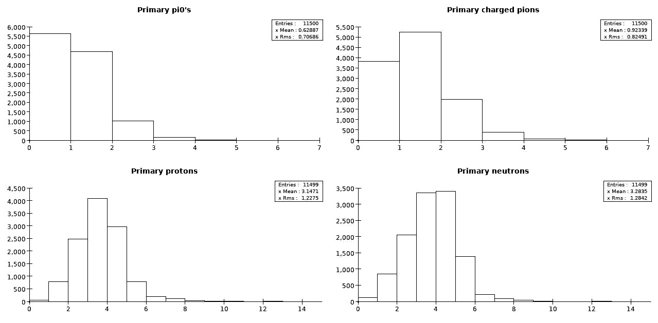
Figure 26: Hadron multiplicity in REDTOP detector. (GenieHadGatto (2012) simulation with Urqmd 3.4)

Despite the large background rate, the occupancy of the events is relatively low, as the kinematics of the final state particles produces only few hits in the detector. Fig. 27 shows the expected number of digitized hits in each sub-detector of REDTOP ($p$+Li$\rightarrow$$\eta X$ with $\eta\rightarrow 3\pi$ and $\eta\rightarrow\gamma\gamma$ are included in the plots).

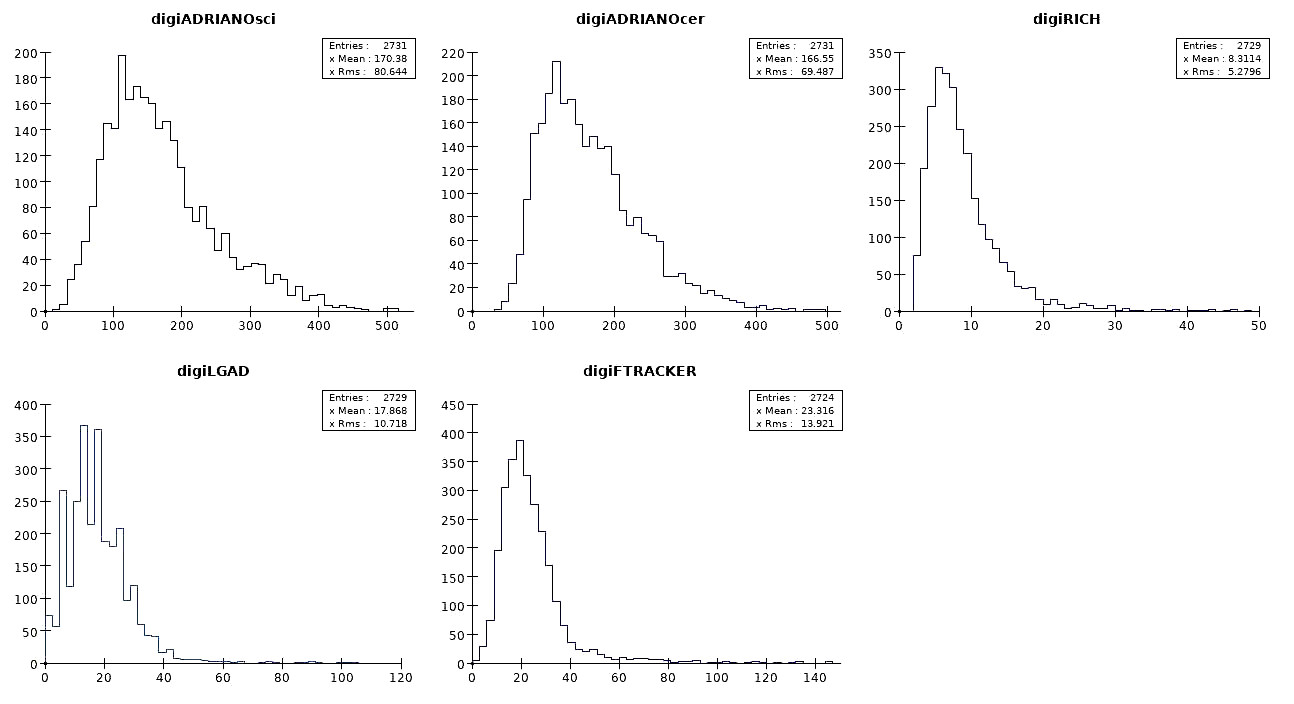
Figure 27: Background occupancy in REDTOP sub-detectors. (Geant4 simulation)

Table  11 summarizes the Monte Carlo estimated average size of digits recorded in each sub-detector for background events. The innermost sections account for less than 13% of the total digitized data.

Digit	FTRACKER	LGAD	RICH	ADRIANO2	ADRIANO2	Total
occupancy				Scint	Cer
Counts	$22.3$	$17.9$	$8.3$	$170.4$	$166.6$	386

Table 11: Average size of digitized data in REDTOP sub-detectors for background events

On the other hand, the most interesting events for dark matter and BSM physics searches have either two leptons or faster pions, with a typical detector occupancy which is 50%-100% larger than the background events.

Assuming a 12-bit digitization for charge and time, and an 18-bit address to identify the struck cell, we estimate that the average size of digitized information obtained from the detector before any trigger is applied is about $1.4\times 10^{3}$ bytes, corresponding to $9.8\times 10^{18}$ bytes/year (or $9.8\times 10^{3}$ petabytes/year). A three-level trigger systems is being considered for REDTOP in order to reduce the data throughput to a more manageable level. The architecture of REDTOP trigger systems is described in detail in the following sections.

VI.7 Level-0 trigger

The selection performed at the Level-0 trigger is based on simple global features of the events produced by $p$-Li inelastic collisions. All the events interesting for New Physics have at least either two leptons or two pions in their final state, in association with at least one energetic photon in the calorimeter. The purpose of the Level-0 trigger is rejecting non-interesting events with a time lag of few tens of nanoseconds. The leptons and pions originating from the decay of the $\eta$ meson are more energetic than those generated by the proton-nucleus interaction, and usually their velocity is above the TCR threshold. The corresponding TOF is, also, smaller. Therefore, the fast Cerenkov signals produced by the LGAD, the TCR and by the ADRIANO2 sub-detectors are the primary input to the Level-0 trigger system. Several requirements need to be met to accept the events:

• a minimum Cerenkov energy from ADRIANO2 integrated over the whole detector;

• at least two clusters in the TCR with energy above threshold and TOF below a defined value;

• the integrated scintillation/Cerenkov signals ratio from ADRIANO2 must be compatible with an electromagnetic shower.

The above requirements are intended to reject the background induced by slower baryons (usually below the Cerenkov threshold of TCR and ADRIANO2) and low-energy gamma which converted in the innermost region of the detector, while accepting the faster leptons and pions from the decay of the $\eta$ meson.

No tracking information is used at the Level-0 trigger, since that would imply implementing some sort of pattern recognition, and, consequently, a longer processing time. The above information, instead, is readily available from the FEE of each detector, and it can be processed in real time by a custom FPGA module. A fast extraction of the scintillation/Cerenkov ratio from ADRIANO2 could be achieved with Field-Programmable Analog Arrays (FPAA) System-on-Chip platforms Asler (2020). The analog processing with FPAA’s will greatly reduce processing latency as well as power consumption. Such a strategy would provide programmable access to analog pulse samples covering the high C/S regions at the start of the pulse and lo C/S regions at the end of the pulse.

The acceptance of the Level-0 trigger for $p$-Li inelastic collisions (background), and several signal events is shown in Table 12.

Inelastic collisions	Input event rate	Average event size	Input data rate	Event acceptance
	Hz	bytes	bytes/s
Background	$7\times 10^{8}$	$1.4\times 10^{3}$	$9.8\times 10^{11}$	21.7%
$\eta\to\pi^{+}\pi^{-}\pi^{0}$	$9.4\times 10^{5}$	$1.5\times 10^{3}$	$1.4\times 10^{9}$	48.6%
$\eta\to\gamma e^{+}e^{-}$	$2.8\times 10^{4}$	$1.5\times 10^{3}$	$4.2\times 10^{7}$	80.6%

Table 12: Level-0 trigger acceptance, event rate, and throughput for inelastic collisions and for typical $\eta$ final states with and without leptons.

Table 13 summarizes average digit sizes, estimated with Monte Carlo techniques, recorded in each sub-detector for QCD background, $p+Li\rightarrow\eta X$ with $\eta\rightarrow 3\pi$ and $\eta\rightarrow\gamma\gamma$ events surviving the Level-0 trigger. The innermost sections account for less than 17% of the total digitized data.

Digit	FTRACKER	LGAD	RICH	ADRIANO2	ADRIANO2	Total
occupancy				Scint	Cer
Counts	$31.9$	$27.0$	$10.3$	$166.6$	$180.4$	416

Table 13: Average digits in REDTOP sub-detectors for background events surviving the L0-trigger

Our studies suggest that, with the Level-0 trigger configured as described above, we can achieve the needed rejection factor of about 20% while preserving a satisfactory efficiency on a large set of interesting physics processes.

The data rate into Level-0 is obtained from Monte Carlo simulations with an estimated reduction factor of $\sim 4.6$ of the event rate and an average event size of $\sim$1.5 Kb, after zero suppression and compression by the DAC. Assuming a 12-bit digitization for charge and time and an 18-bit address to identify the struck cell, a collision rate of 700 MHz, we conclude that the average rate of the data sent to the Level-1 trigger is about $\sim$230 Gb/s. Such a data rate can be comfortably transmitted by a network of a few hundred optical fiber links. Because all data from the detector are continuously digitized in the front-end and immediately transmitted to the following stages, trigger latency is not expected to be a problem, at least to first order. Therefore the Level-0 logic can be heavily pipelined. Although a new event will arrive, on average, every 1.4 ns, the time taken to make a decision on a specific event can be much longer, possibly of the order of hundreds of nanoseconds.

VI.8 Level-1 trigger

In contrast with the global aspects of Level-0 input, the Level-1 rejection is based on local information obtained directly from the sub-detectors. That requires the implementation of at least a low-level pattern recognition and clusterization of the hits. The algorithms implemented for the present studies are intended to reduce the background from baryons as well as from photons converting into an $e^{+}e^{-}$ pair in the innermost region of the detector. The set of requirements for the Level-1 trigger are listed below, grouped by the specific type of background targeted:

Baryon rejection

• at least three clusters in the LGAD tracker, separated by a distance of 4.5 mm or larger;

• at least two groups of hits with three LGAD clusters and one TCR cluster, consistent with oppositely charged particles, and with TOF below a defined threshold;

• the integrated energy in the TCR for positive and negative tracks has to exceed a defined threshold;

• at least three ADRIANO2 clusters with scintillation/Cerenkov ratio consistent with a non-baryonic particle.

$\gamma\to e^{+}e^{-}$ rejection

• No clusters in the FTRACKER, associated to two oppositely charged tracks, separated by less than 3 mm in the x-y plane and 12 mm in the z-direction;

• No clusters in the LGAD associated to two oppositely charged tracks separated by a distance shorter than of 4.5;

The particle identification in ADRIANO2, at the Level-1 trigger, could be implemented in a two-layer Artificial Neural Network (ANN) with a dedicated Field-Programmable Analog Arrays, receiving the input from the C/S system implemented in the Level-0 trigger. The choice of the sample to send to the ANN can be programmed in order to fine tune the trigger system and to satisfy the requirements of a particular physics run. The technique would be capable to optimize the C/S separation between hadronic and electromagnetic showers at run time. The output of the ANN would be digitized and recorded with the channel, with an estimated reduction of information of about one-order of magnitude.

The acceptance of the Level-1 trigger for $p$-Li inelastic collisions (background), and for several topologies of signal events, is shown in Table 14. Assuming a 12-bit digitization for charge and time and an 18-bit address to identify the struck cell, the Level-1 input data rate is $\sim$230 Gb/s. Factorizing the event reduction of $\sim 60$ (cf. Table 14), we conclude that the expected average rate of data sent to the Level-2 trigger is about $\sim$3.8 Gb/s. Such a data rate can be comfortably transmitted by a network of a few hundred optical fiber links. A significant challenge of the REDTOP trigger will be to design specialized processors to achieve the needed rejection factor of under 2% by reconstructing proto-tracks with high efficiency, at an event rate of 100 KHz. We believe that this selectivity can only be achieved with specialized hardware, possibly based on massive use of FPGAs.

To gain more time to process each event, we can adopt a time multiplexing strategy. We anticipate that events will be distributed to a bank of identical processors in a round-robin fashion. The larger the number of processor, the more time each one of them will have to process one event. A time multiplexing of factor of 10 will allow each processor 5 microseconds, on average, to process each event, which seems adequate for the task.

As a comparison, a demonstrator of the Level-1 tracking trigger for CMS Phase II has recently shown that ten identical, FPGA-based, processors, housed in a single ATCA crate and operated in a time-multiplexing mode, can process events coming at a rate of 40 MHz from a unit corresponding to 1/48 of the CMS tracker. Each unit contained the order of 500 hits and was carried by about 400 fibers. All the tracks with a $P_{t}$ above 3 GeV/c could be reconstructed with high efficiency and a latency of a few microseconds. The rates processed and the complexity of the problem are on the same level as expected for REDTOP Level-1 trigger.

Process	Input event rate	Average event size	Input data rate	Event acceptance
	Hz	bytes	bytes/s
Inelastic collisions	$1.5\times 10^{8}$	$1.5\times 10^{3}$	$2.3\times 10^{11}$	1.7%
$\eta\to\pi^{+}\pi^{-}\pi^{0}$	$4.6\times 10^{5}$	$1.6\times 10^{3}$	$6.9\times 10^{8}$	10.9%
$\eta\to\gamma e^{+}e^{-}$	$2.3\times 10^{4}$	$1.6\times 10^{3}$	$3.6\times 10^{7}$	64.6%

Table 14: Level-1 trigger acceptance for inelastic collisions and for a typical $\eta$ final states with and without leptons.

Table 15 summarizes the Monte Carlo-estimated average size of digits which would be recorded in each sub-detector by QCD background, $p$+Li$\rightarrow$$\eta X$ with $\eta\rightarrow 3\pi$ and $\eta\rightarrow\gamma\gamma$ events surviving the Level-1 trigger. We note that the innermost regions of the detector account for less than 17% of the total digitized data.

Digit	FTRACKER	LGAD	RICH	ADRIANO2	ADRIANO2	Total
occupancy				Scint	Cer
Counts	$34.1$	$28.9$	$10.7$	$178.0$	$193.2$	446

Table 15: Average digits in REDTOP sub-detectors for background events surviving the L1-trigger

VI.9 Level-2 trigger

The Level-2 trigger aims at positively identify the underlying physics process and, therefore, it relies heavily on the topology of the final state. The algorithm implemented requires a fully reconstructed event, including: a) the identification of the target foil where the primary interaction occurred, b) the approximate reconstruction of tracks and calorimetric showers, c) identification of potential secondary vertexes. The requirement on the final state topology for discriminating the event at the Level-2 trigger are:

• at least two fully identified leptons;

• two oppositely charged pions and two calorimetric showers;

• four pions;

• any two oppositely charged tracks with a secondary vertex detached by more than 5 cm from the primary interaction.

The acceptance of the Level-2 trigger for $p$-Li inelastic collisions (background), and several topologies of signal events is shown in Table 16. The Level-2 processor farm will receive 2.5 MHz of events, equivalent to a data rate of $\sim$3.8 GB/s, from Level 1. These events need to be reconstructed, filtered and formatted for permanent storage. We assume that this task can be completed by using less than 100 ms of CPU time and that, consequently, a farm of 2000 CPUs should be adequate for the job.

We note that this same processor farm can be used for “data production” when the experiment is not taking data.

Factorizing an event reduction of $\sim 4.5$ as being estimated with Monte Carlo simulations (cf. also Table 16), we conclude that the average output data rate sent to permanent storage is $\sim$0.9 Gb/s or about$\sim 9$ PB/year, which we consider manageable.

Process	Input event rate	Average event size	Input data rate	Event acceptance
	Hz	bytes	bytes/s
Inelastic collisions	$2.5\times 10^{6}$	$1.5\times 10^{3}$	$3.8\times 10^{9}$	22.2%
$\eta\to\pi^{+}\pi^{-}\pi^{0}$	$5.0\times 10^{4}$	$1.7\times 10^{3}$	$8.5\times 10^{7}$	82.7%
$\eta\to\gamma e^{+}e^{-}$	$1.5\times 10^{4}$	$1.7\times 10^{3}$	$2.5\times 10^{7}$	94.3%

Table 16: Level-2 trigger acceptance for inelastic collisions and for typical $\eta$ final states with and without leptons.

Table 17 summarizes the Monte Carlo estimated average digits recorded in each sub-detector for QCD background, $p$+Li$\rightarrow$$\eta X$ with $\eta\rightarrow 3\pi$ and $\eta\rightarrow\gamma\gamma$ events surviving the Level-2 trigger.

Digit	FTRACKER	LGAD	RICH	ADRIANO2	ADRIANO2	Total
occupancy				Scint	Cer
Counts	$36.1$	$30.6$	$11.6$	$190.8$	$206.0$	475

Table 17: Average digits in REDTOP sub-detectors for background events surviving the L2-trigger

VI.10 Digitize and Compress: summary of trigger performance

The task of the REDTOP trigger systems is to reduce the event rate from the $p$-Li total inelastic collision rate of$\sim 7\times 10^{8}$ Hz down to about $3$ MHz of events to be permanently recorded. Assuming a 12-bit digitization for charge and time and an 18-bit address to identify the struck cell, we conclude that the average size of the final event surviving all levels of trigger is about $1.6\times 10^{4}$ bytes. A summary of the expected data throughput is presented in Table 18. Such yield will produce an output data rate of $\sim$0.9 Gb/s or about$\sim 9$ PB/year, which we consider manageable.

The needed $\sim 2.3\times 10^{3}$ reduction in event rate is achieved by three trigger stages. These three stages are preceded by a digitization and compression (DAC) stage. The DAC stage is directly connected to the front-end of the detector. Level-0 and Level-1 are located off the detector. A fiber optics network delivers data from the DAC to Level-0 and from Level-0 to Level-1. The events filtered by Level-1 are delivered to Level-2, a processor farm that performs event building, reconstruction, formatting, and classification. A further rate reduction can possibly be achieved at Level-2, before permanent recording, if needed. Table 18 summarizes data and event rates into and out of the different stages.

Trigger	Input event rate	Event size	Input data rate	Event rejection
stage	Hz	bytes	bytes/s
Level 0	$7.\times 10^{8}$	$1.4\times 10^{3}$	$9.8\times 10^{11}$	$\sim$4.6
Level 1	$1.5\times 10^{8}$	$1.5\times 10^{3}$	$2.3\times 10^{11}$	$\sim$60
Level 2	$2.5\times 10^{6}$	$1.5\times 10^{3}$	$3.8\times 10^{9}$	$\sim$4.5
Storage	$0.56\times 10^{6}$	$1.6\times 10^{3}$	$0.9\times 10^{9}$

Table 18: Data and event rates for different stages

Future improvement in the detector design are expected to reduce further the background. In particular, we foresee the adoption of a ultra-thin vertex detector (cf. Sec. VI.4.1) which will improve considerably the rejection factor of the Level-1 trigger.

VI.11 The Computing Model

The computing model for REDTOP is adapted from what is currently implemented for several High Energy Physics experiments out of a DOE or NSF major facility. It aims to paste together the pieces of an end-to-end infrastructure and software that enables the delivery of the final data-products to the researchers at the different institutional research partners.

The REDTOP experiment operates in a typical beam environment where the inelastic interaction rate of the proton beam with the target is  1 GHz. Level-0 and Level-1, implemented in hardware, will reduce such a large rate by a factor of $\sim 104$ before sending the data to a local compute-farm for the Level-2 trigger and preliminary reconstruction. We expect approximately 2.5 PB of production-quality experiment data and approximately 2 PB of processed data to be generated each year via the acquisition and reconstruction of the experimental output together with the required simulations. In order to accommodate these storage requirements, the Fermilab (FNAL) facility is needed to provide long-term tape storage during each year of operation and a disk allocation on FNAL’s dCache for staging and distributing data elsewhere. In addition to FNAL, REDTOP will a leverage an allocation on the Open Science Connect service which can provide 100 TB-scale ephemeral storage (Stash) for jobs to the Open Science pool.

In terms of compute requirements, REDTOP employs a single-core computational workflow which has proven to be well suited for the distributed High Throughput Computing (dHTC) environment of the Open Science Farbic of services. The computing model here aims to facilitate reconstruction of the expected flow of data from the full experimental apparatus along with the suite of required Monte Carlo simulations. Extrapolating from REDTOP jobs currently running on Open Science pool, it is estimated that the we would need approximately 90 million core hours annually; 55 million core-hours for Monte Carlo jobs and 35 million core-hours for data reconstruction jobs.

With the above considerations in mind, we assume that the output data stream from the Level-2 farm will be staged at Fermilab’s dCache storage and, eventually, pre-processed on site. The process will require an allocation on the lab’s General Purpose Grid (GPGrid) with local file access on dCache enabled via a POSIX-like interface over an NFS mount. dCache will primarily serve as a high speed front-end ephemeral storage to provide access to data stored on tape. Since direct access to tape is limited to on-site infrastructure, staging on dCache first enables downstream access by off-site resources. In order to increase the flexibility of the model and to offer more optimal implementations to the participating institutions, the following options are considered and discussed below.

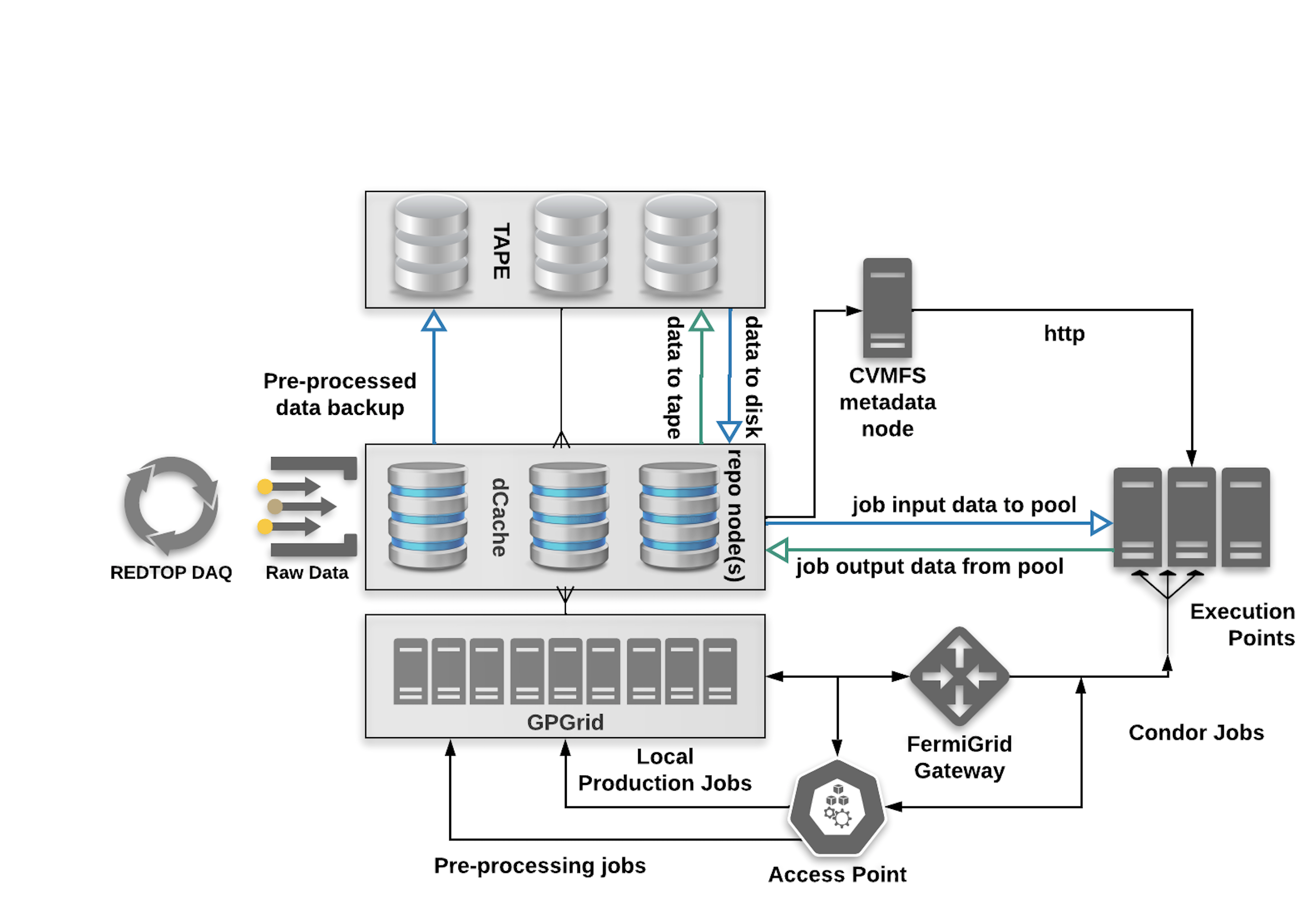
Figure 28: The REDTOP compute workflow out of Fermilab. Experimental data out of the REDTOP DAQ are stored on FNAL’s dCache from where they can be pre-processed for level-2 triggers and preliminary reconstruction on the local cluster. Data are then stored on tape. An access point at FNAL, an HTCondor submit node, can submit jobs to the Open Science pool. Data in this scheme are delivered directly from dCache after being staged first on tape.

The collaboration will process the bulk of the experimental results via HTCondor jobs submitted to FermiGrid or Open Science pool from a lab access point (submit node). An example of a job submission workflow for REDTOP at FNAL is shown in Fig. 28. A submit host sends jobs to the pool while data are delivered to the remote compute sites (execution points) by first staging them on dCache and then transferring them to the remote execution points via a protocol like XRootD or http. It is proposed that Fermilab also deploys a data origin repository for REDTOP in the distributed CernVM File System (CVMFS) which will deliver input data to remote compute sites using OSG’s federation of caches Weitzel et al. (2019). The OSG data federation (OSDF) service replicates data needed by a project on a cache in regional proximity to a compute site. When a user job requests a dataset or a software bundle via a collaboration specific CVMFS path in the execution script, it fetches the data from the nearest cache instead of the origin. This minimizes the flight path to the execution point (worker node) and improves the runtime efficiency of the job. The software stack, which includes the GenieHad and Geant4 Monte Carlo software as well as the reconstruction framework, can also be distributed out of the same repository, however there is an alternative option to host the software origin in the OASIS repository - OSG’s Application Installation Service. Any output data designated for long term storage can then be archived back to tape at Fermilab by first transferring the files back onto dCache using the same protocols as above.

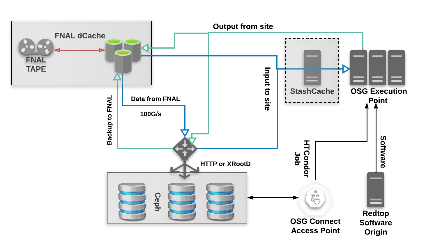
Figure 29: The REDTOP compute workflow using an Open Science Connect access point, a HTCondor job submit node. This entry point provides a broader access to the research community for job submissions to the Open Science pool. Data from FNAL can be pre-staged on the OSG Connect storage - Stash - although that is not strictly necessary if the user has credentials to access Fermilab resources as in this case the job on the execution point can request data directly from the FNAL’s dCache disk.

The collaboration will continue to leverage the OSG Connect entry points at the University of Chicago to launch reconstruction or simulation jobs to the Open Science pool. OSG Connect provides a collaborative environment for a multi-institutional partnership such as REDTOP, where researchers from the individual institutions can request accounts to the access point via an online portal. Users can then join the REDTOP project, gain access to the project’s shared directory on the OSG distributed storage (Stash) and submit jobs to the Open Science pool. Stash, a Ceph filesystem storage system, provides temporary storage capacity for OSG projects and can distribute data to remote execution points in the Open Science pool over CVMFS or via a direct copy using XRootD or http.

REDTOP has the option to make use of Stash to pre-stage input files and to store the processed output files from the jobs before distributing them to various endpoints of the collaboration including archiving them back to tape at FNAL. Figure 29 shows such an example of a data processing workflow using OSG Connect. Users submit HTCondor jobs to the Open Science pool from the submit host (the access point). Input data can be delivered to the execution point either from stash or via a gfal-copy from dCache at Fermilab. Similarly, the output data can be copied back to stash or to Fermilab’s dCache and eventually to tape. Note that user access to the files at Fermilab will require them to authenticate with their credentials to the storage endpoint.

While not in the critical path to the processing campaign of the experimental data, the REDTOP collaboration can augment the availability of computing cycles by fostering the creation of a dedicated resource pool via allocations on facilities at member institutions. This is similar to the general purpose Open Science pool; user submitted HTCondor jobs run as payloads in pilots launched to these dedicated execution points by the Open Science gWMS factory via entry points (gateways) that can be hosted by OSG or deployed locally at the institutional edge infrastructure.

The approach described above constitutes a minimalist compute-storage model that will meet the requirements of REDTOP if the appropriate scale of the annual storage requirements is met at Fermilab. A distributed storage model can also be considered which requires participating institutions to contribute storage to the collaboration. Such model requires the introduction of a data management appliance/service that will coordinate the data placement into the different storage endpoints (RSE: Rucio Storage Endpoint) and manage the mobility across sites and execution points at the Open Science Pool.

This model is briefly described in the upper panel of Fig. 30. Data collected by the experiment are ingested into the Rucio database and distributed into various storage end-points using the File Transfer Service (FTS). The metadata stored in the Rucio database include information such as the size, institutional location, scope of the file and directory path of a file. This process facilitates the distribution of the entire experimental output, reducing the storage footprint on the primary site (FNAL) which can still maintain post level-2 data on tape. Portions of the experimental output will then be readily available to individual institutions for on-site reconstruction or analysis besides the capability to deliver the data to jobs at the Open Science pool on demand.

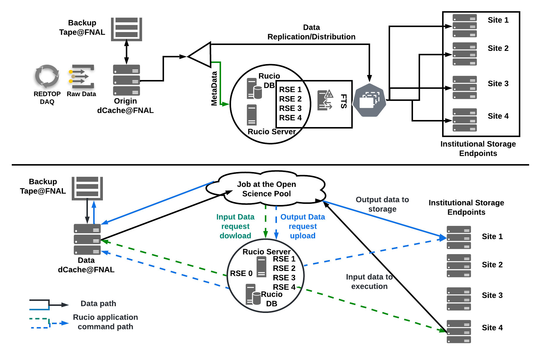
Figure 30: A compute-storage model for REDTOP where a data management appliance, Rucio, is used to distribute data from an Origin (FNAL) to dedicated institutional storage end-points. When jobs at the Open Science Pool request an input file, they query the Rucio server for a download. The server then coordinates the proper download location of the file to the execution point. The process is reversed when uploading files to the storage-end points (RSEs) which also updates the catalog maintained by Rucio.

This scenario is described in the lower panel of Fig. 30, where an HTCondor job running at a remote execution point can request an input file from the Rucio server which mediates the delivery of the file to the job from the appropriate RSE that has it. The process can be reversed by uploading an output file back to a storage end-point which also updates the dataset catalog in the Rucio database. This process can be considered supplementary to the capabilities offered by the OSDF service of caches. The latter delivers datasets in proximity to a nearby execution points but only in the context of a HTCondor job submitted by a user from an access point such an FNAL or OSG Connect. A data management service like Rucio will afford the opportunity to the collaboration’s research partners to process data in local facilities or dedicated Open Science execution points even in the absence of a nearby OSDF cache.

VII The Simulation Framework

VII.1 The event generator: $GenieHad$

An experiment aimed at detecting faint signals of New Physics in a harsh hadronic environment presents several challenges concerning the knowledge of the detector response and of the topology of the physics events. Considering the significant number of inelastic nuclear collisions produced in REDTOP targets, a reliable simulation of the hadronic interactions between the proton beam and the nucleons in the target is of paramount importance to estimate the background and, consequently, the sensitivity to New Physics. Among the simulation packages presently available to the experimenters in High Energy and Nuclear physics, Geant4 is by far the most widely used and its particle transport mechanism is, probably, unsurpassed. However, processes occurring at energies below $\sim 10$ GeV need specific hadronic generators and framework for the following reasons. Hadronic interactions governing the beam-target scattering in that energy range occurs predominantly via the formation and the decay of intra-nuclear baryonic resonances. The treatment of such processes is very complex, and it requires a non-perturbative approach. Furthermore, excited nuclei could de-excite into nucleons and nuclear remnants, which could, subsequently, interact with the detector.

The approach followed in the present work is of separating the simulation of the primary interaction from the transport of the secondary particles throughout the detector. More specifically, the primary interaction between the beam and the nuclear matter contained in the target is simulated with a specialized event generator which would reproduce the scattering and the de-excitation of the nucleus according to one or more nuclear transport models, evaporation/fragmentation/fission and final de-excitation models. In the following step, those particles and ions are propagated throughout the material volumes of the detector using the Geant4 package.

Several standalone intranuclear scattering and transport models have been implemented in the last few years to simulate the interaction between a hadron or an ion and a nucleus. Given the complexity of the underlying models, those programs are usually developed and maintained by nuclear theorists. From the experimental point of view the packages currently available have two important deficiencies:

1. The nuclear target is an isolated nucleus surrounded by vacuum (namely, re-scattering in the target is not considered);

2. Except for one caseHirtz et al. (2020), the nucleons generated in the final state is considered as isolated (i.e, un-aggregated) particles, rather than as clusters of, eventually excited, ions.

To overcome such limitations, the $GenieHad$Gatto (2012) event generator package has been developed. $GenieHad$ is an extension of the $Genie$ framework Andreopoulos et al. (2010) that is widely used in the neutrino community, as it relies on its geometry package and its architecture. The heart of $GenieHad$ is a collection of twenty modules interfacing external hadronic simulation packages Buss et al. (2012); Hirtz et al. (2020); Bleicher et al. (1999); Nara, Yasushi (2019); ESP (2018); Ehehalt and Cassing (1996); Sjöstrand et al. (2015) to $Genie$. The primary nuclear interaction is deferred by the corresponding $GenieHad$ interface to the external hadronic generator which performs the scattering according to the parameters specified by the user. Once the scattering engine has completed its process, the final products are returned to $GenieHad$ which prepares them for the following steps. These are, usually, a) the clusterization of the individual nucleons into nuclear remnants or fissioned ions, alpha particles, etc, b) the de-excitation and/or evaporation of eventual remnants with positive binding energy. Such final steps are performed by a set of dedicated simulation packages. A list of the nuclear, electromagnetic, clusterization and de-excitation models currently implemented in $GenieHad$ is presented, in Tables 19, 20, 21, and 22.

Package	Model	Type
Urqmd Bleicher et al. (1999)	QMD	Microscopic many body approach
Incl++ v6.2 Hirtz et al. (2020)	INCL	Intranuclear cascade
Gibuu v2019 Buss et al. (2012)	BUU	time evolution of Kadanoff–Baym-equations
PHSD v 4.0 Ehehalt and Cassing (1996)	HSD	covariant transport with NJL-type Lagrangian
Jam v1.9 Nara, Yasushi (2019)	Cascade/RQMD.RMF/BUU	Multi-model - hybrid approach
Dpmjet-III Roesler (2005)	Dual Parton/ perturbative QCD	Multi-model approach
Pythia 7, 8Sjöstrand et al. (2015)	LUND	string hadronization model
IAEA tablesORNL (2022)	LUT of measured cross sections	Look-up tables based on ENDF (by IAEA)
IntranukeTena-Vidal et al. (2022)	Parametric
ALPACAHarland-Lang et al. (2019)	Alpaca	Bremsstrahlung of Axion-Like-Particles (ALPs)

Table 19: Nuclear scattering models available in GenieHad Gatto (2012).

Package	$\gamma$	N, p, He	IMF	Fission
	emission	model	Model	model
Abla07Kelic et al. (2009)	yes	Weisskopf-Erwig	no	Fokker-Plank
Abla++ Rodríguez-Sánchez et al. (2015)	yes	Weisskopf-Erwig	no	Fokker-Plank
GEM Furihata (2000)	no	Weisskopf-Erwig	Weisskopf-Erwig	parametric
Gemini++ Charity et al. (2001)	no	Hauser-Feshbach	Transition state	Transition state model
Evapor Abdel–Waged et al. (2012)	no	Weisskopf-Erwig	no	parametric
SMM Baznat et al. (2020)	no	Weisskopf-Erwig	Weisskopf-Erwig	Statistical Multifragmentation

Table 20: De-excitation, evaporation, fission models available in GenieHad Gatto (2012).

Package	Type
Geant4 EM physics Agostinelli et al. (2003)	Parametric
LELAPS Langeveld (2005)	Parametrized shower simulation

Table 21: Electromagnetic interaction models available in GenieHad Gatto (2012).

Package	Model
CoalescenceBleicher et al. (1999)	GEM based Phase-Space Coalescence
KAWAbdel–Waged et al. (2012)	Urqmd based Phase-Space Coalescence

Table 22: Clusterizer models available in GenieHad Gatto (2012).

In the $GenieHad$’s architecture, because of the approach described above, the environment of the event (geometry of the apparatus, materials, beam profile and composition, targets, etc.) is taken care of by the underlying framework (namely, $Genie$), while the scattering at the microscopic level is performed by the external engine, which is called at run-time according to the selected transport model. One of the main advantage of this approach is the possibility to compare the outcome of different nuclear transport models under identical conditions, and in particular, within the same geometry and the same beam parameters. By repeating the simulation and comparing the results from several models, one can evaluate the robustness of the procedure and estimate the uncertainties of observables.

In the contest of the studies performed for this work, $GenieHad$ was employed to generate signal and background events according to physics of the SM. In order to study physics BSM, the $\eta$ and $\eta^{\prime}$ mesons produced (along with other mesons and baryons generated by the fragmentation of the target), are subsequently decayed by a special $Geniehad$ module reproducing the process under study. Nineteen such modules have been developed, each incorporating the decay amplitude for that particular theoretical model. More details on the event sets being produced can be found in the respective subsections of Sec. VIII through XIV

VII.2 The particle transport software: $slic$

The second step of the simulation consists of transporting the particles and nuclear remnants generated in $GenieHad$ throughout the target and the the detector. This task is performed by Geant4, via the $slic$ package, which manages the geometry and the event input-output. $slic$Graf and McCormick (2006) was initially developed by the SID Collaboration within the ILC framework. It is currently used for the simulation of the events by the HPS experimentAdrian et al. (2018) at JLAB. A very detailed geometry is implemented in a gdml format and an extended gdml schema is used for the segmentation of sensitive detectors. For the sake of this work, most of the passive material, relevant for the determination of the multiple scattering, is also taken into account. Furthermore, REDTOP uses a proprietary version of $slic$ including, among other things, the physics of optical photons, which is necessary for the correct simulations of the signal of ADRIANO2 calorimeter. The results of this step is a collection of “hits” which carry the information of the energy deposition and its location in the sensitive volumes of the detector.

VII.3 The reconstruction and analysis software: $lcsim$

The software framework which implements the simulation of the response of the experimental apparatus, after the particle transport and the energy deposition in the apparatus is completed by Geant4, is $lcsim$Graf et al. (2012). This software framework is a java based package, initially developed by SID Collaboration within the ILC framework and also used by the HPS experimentAdrian et al. (2018) at JLAB. The reconstruction in lcsim proceeds according to the following steps:

• Digitization of the hits produced by Geant4, based on the simulated response of the front-end electronics;

• Simulation of the algorithms implemented in the Level-0 trigger for fast rejection of the background;

• Pattern recognition;

• Simulation of the algorithms implemented in the Level-1 trigger;

• Track reconstruction from the digits collected in the tracking system;

• Shower reconstruction in the $TCR$ and $ADRIANO2$;

• Simulation of the algorithms implemented in the Level-2 trigger for rejection of the background based on the event topology;

• Final analysis of the event.

Further details are given in the next section.

VII.4 The simulation strategy

This section describes in detail the strategy implemented in the simulations, along with the parameters used.

VII.4.1 Beam parameters

A collimated proton beam with a Gaussian energy spread and transverse profile was implemented in $Genie$ + $GenieHad$. In order to preserve the validity of the results of the studies with a broader range of accelerator configurations, we have used the following, very conservative, beam parameters:

• $E_{kin}$ = 1800 MeV

• $\sigma_{E_{kin}}$= 0.9%

• $\sigma_{x},\,\sigma_{y}$ = 1 mm, 5 mm

• Beam halo: 4.5 mm $\times$ 4.5 mm

VII.4.2 Digitization

The first step of the reconstruction performs the digitization of the hits found in the four sub-detectors. The following experimental effects are taken into account for each of them:

Fiber tracker

• Efficiency of individual fibers;

• Photo-detector efficiency ($pde$) and energy response of the SiPM;

• Amplification and discrimination of the signal.

Central tracker (LGAD tracker)

• Single pixel efficiency;

• Diffusion and cross-talk among nearby pixels;

• Amplification and discrimination of the signal;

• Smearing of the time of formation of the hit.

Threshold Cerenkov Radiator

• Parametrization of the detector response based on the results of T1604 test beam.

ADRIANO2

• Parametrization of the detector response based on the results of T1604 experiment.

VII.4.3 Simulation of the trigger systems

The algorithms for the three trigger levels have been fully implemented in $lcsim$. A detailed description of REDTOP trigger system can be found in Sec. VI.5.

VII.4.4 Pattern recognition and PID

Given the novelty of the detector technologies proposed, REDTOP does not yet have, as of this writing, a full pattern recognition in place. Consequently, a cheating strategy has been implemented, where the digits are assigned to a particle using the Monte Carlo truth. The same situation holds for the PID, which is assigned to each reconstructed particle using a LUT, storing realistic values of efficiency and mis-identification probabilities. The latter have been evaluated with Monte Carlo techniques and known experimental results.

VII.4.5 Track reconstruction in the Fiber Tracker and in the Central Tracker (helix fit and Kalman filter)

A full helix fit of the tracks in a solenoidal magnetic field is performed in the tracking systems. Multiple scattering and energy loss in materials traversed by the tracks are taken into account in the covariance matrix. Only those tracks successfully fitted and with a satisfactory $\chi^{2}$ are passed to the next step of the reconstruction. In addition to the helix fit, a full Kalman filter has been implemented, although it has not been used for the studies presented here.

VII.4.6 Shower reconstruction in the TCR and ADRIANO2 calorimeter (parametric)

The TCR, which is located immediately in front of ADRIANO2, has also the functions of a pre-shower for the latter. As mentioned in Sec. VII.4, several test beams have been conducted with ADRIANO2 prototypes by T1604 Collaboration. To speed up the simulations for the studies presented in this work, a parametric response of the detector has been implemented, based on the results of those tests.

VIII Sensitivity Studies to Physics Beyond the Standard Model

In this section we present the results of the physics studies performed to estimate the sensitivity of REDTOP to several benchmark BSM processes and several theoretical models. The studies are based on the Snowmass-2021 detector layout, described in some details in Sec. VII. Such studies have two goals: a) presenting the physics case for a $\eta/\eta^{\prime}$-factory; b) finding possible improvements of the experimental apparatus and in which way they would impact most strongly the discovery potential of REDTOP. This section is organized as follows. In Sec. VIII.1 we derive the formulae used to determine the branching ratio sensitivity. Sec. VIII.3 and VIII.2 describe the methodology used to simulate the signal and background samples. In Sec. IX through XII we focus on the sensitivity studies for the four portals connecting the Dark Sector with the Standard Model. We proceed first by evaluating the sensitivity to the branching ratio of the relevant processes, and then, we apply those results to benchmark several theoretical models. In Sec. XIII we present our results on sensitivity studies relevant for testing the discrete symmetries of the Standard Model. The symmetries considered in this work are: $C$ and $CP$, Lepton Flavor Violation ($LFV$), and Lepton Universality. Finally, in Sec. XV we discuss the results, and try to identify the possible improvements to the experiment.

VIII.1 Estimation of the sensitivity curves

In this section we derive the formulae needed to estimate the branching ratio sensitivity as well as to a generic theoretical models. More specifically, assuming that the model is based on a (set of) parameter(s) $\bar{g}$, usually the coupling constant(s) of the amplitude(s) involved, by sensitivity we define the minimum value(s) of $\bar{g}$ measurable at REDTOP with a signal which is three times larger than the background fluctuations. For an experiment at a meson factory, where the $\eta/\eta^{\prime}$ are hadro-produced, we expect a large background from QCD contaminating most of the final states. The sensitivity is define as the value of $\bar{g}$ such that:

$$S_{min}(\bar{g})=3\times\sqrt{B}$$ (102)

where: $S_{min}$ is the minimum number of signal events reconstructed and surviving the final selection, while $B$ is the number of background events.

If$N_{\eta}$ ($N_{\eta^{\prime}}$) is the number of $\eta$ ($\eta^{\prime})$ mesons produced and $N_{ni}$ is the number of inelastic nuclear interactions between the beam and the target, then:

$$S_{min}(\bar{g})=N_{\eta}\times Br(\bar{g})\times\epsilon_{reco}\,,$$ (103)

$$B=N_{ni}\times\epsilon_{bkg}$$ (104)

where $Br(\bar{g})$ and $\epsilon_{reco}$ are, respectively, the branching ratio and the reconstruction efficiency for that channel, while $\epsilon_{bkg}$ is the probability that a Standard Model event will survive all analysis cuts. From. Eqs. 102-104, we define the branching ratio sensitivity as:

$$sensitivity(Br(\bar{g}))=\frac{3\times\sqrt{N_{ni}\times\epsilon_{bkg}}}{N_{\eta}\times\epsilon_{reco}}$$ (105)

Assuming an incoming beam with $10^{11}$ POT/sec and an integrated proton yield of $3.3\times 10^{18}$ POT (that, according to the analysis performed in Sec. VI.1, is achievable with an effective running time of 12 months), the expected total yield of $\eta$/$\eta^{\prime}$ and of inelastic proton collisions, are summarizes in Table 23. In those calculations, we conservatively assumed a value of 0.49% for the production probability, as obtained from the Urqmd model in $GenieHad$, instead of the value of 0.70% obtained by averaging the results from several generators (cf. Tab.8). This is also consistent with our final choice of $Urqmd$ for the generation of the events for the sensitivity studies presented below (see, also, Sec. VIII.2).

	Total yield for $E_{kin}$=1.8 GeV
$N_{\eta}$	$1.1\times 10^{14}$
$N_{\eta^{\prime}}$	$0$
$N_{ni}$	$2.5\times 10^{16}$

   Total yield for $E_{kin}$=3.6 GeV $N_{\eta}$ $5.9\times 10^{14}$ $N_{\eta^{\prime}}$ $7.9\times 10^{11}$ $N_{ni}$ $3.2\times 10^{16}$

Table 23: Expected event yield at REDTOP for $3.3\times 10^{18}$ POT, estimated with the Urqmd module of $GenieHad$ (see Sec. VII.1 for details on the estimation method).

The values of $\epsilon_{reco}$ and $\epsilon_{bkg}$ have been determined for each of the analyses presented in the remaining of this article. Once a master formula for $Br(\bar{g})$ is obtained for a particular theoretical model, then Eq. (105) can be used to extract the experimental sensitivity to the parameter(s) $\bar{g}$.

VIII.2 Standard Model background

As discussed in Sec. VII.1, several nuclear scattering generators are available in $GenieHad$. For the studies presented in this work, we have extensively examined two of them: $Urqmd$ and $Incl++$. We generated about $2\times 10^{9}$ $p+Li\rightarrow X$ inclusive inelastic events with each generator, and analyzed their outcome. We concluded that our sensitivity studies are not appreciable affected by which of the two is chosen. We decided to use $Urqmd$ to generate the remaining event sample, as, in spite of being computationally more intensive than $Incl++$, it is widely regarded by the intermediate energy community the most effective in simulating the nuclear scattering at the energies of interest for REDTOP. An integrated sample of about $5\times 10^{10}$ events was finally produced, corresponding to $2\times 10^{12}$ POT, or 1/500,000 of the expected beam integrated current. The final nucleons from $Urqmd$ were, subseqently, clusterized into nuclear remnants by the KAW clusterizerAbdel–Waged et al. (2012) and, finally, de-excite and evaporated with $ABLA\,v7$ Kelic et al. (2009).

At present, only few decays of the $\eta/\eta^{\prime}$ mesons currently implemented in Geant4. Therefore, the missing exclusive $\eta/\eta^{\prime}$ processes needed to estimate the signal and the background were individually generated using $GenieHad$.

The events generated with $GenieHad$ were, subsequently, processed with Geant4, to simulate the response of the detector. The digitization and reconstruction strategy are described in detail in Sec. VII.4. Finally, the background was merged with the signal during the analysis step, and re-weighted to take into account eventual differences in the number of POT’s.

VIII.3 Generation of signal events

The studies discussed in the present work refer only to the production and decay of the $\eta$-meson. Similar studies for the $\eta^{\prime}$-meson production and decay are planned, and will be published in a future work.

The $Urqmd$ sample described above sample consists of about $2.35\times 10^{8}$ $p+Li\rightarrow\eta+X$ events which were extracted and used as input to $GenieHad$ to generate exclusive decays corresponding to the process under study. As already stressed above, the vast majority of $\eta$-mesons is produced by the decay of intra-nuclear resonances with masses below 2 GeV. Therefore, those mesons have only a modest boost in the laboratory frame. As shown in Fig. 18, about 40% of the $\eta^{\prime}$s have a kinetic energy less than 100 MeV. In order to optimize the computing time, sub-samples of the full $\eta$-set were prepared for the individual analyses, while the entire background sample was used. The $\eta$-meson was further decayed in $GenieHad$, with a decay amplitude derived from the theoretical model being benchmarked. The full simulation process is described in detail in Sec. VII.4.

IX Sensitivity to the Vector portal

The Vector portal can be probed via radiative decays of the $\eta$-meson and its subsequent decay into a lepton-antilepton $\ell\bar{\ell}$ pair or into two pions. The following processes have been considered in this work:

• $p+Li\rightarrow\eta+X\;with\;\eta\rightarrow\gamma A^{\prime}\;and\;A^{\prime}\rightarrow e^{+}e^{-}$

• $p+Li\rightarrow\eta+X\;with\;\eta\rightarrow\gamma A^{\prime}\;and\;A^{\prime}\rightarrow\mu^{+}\mu^{-}$

• $p+Li\rightarrow\eta+X\;with\;\eta\rightarrow\gamma A^{\prime}\;and\;A^{\prime}\rightarrow\pi^{+}\pi^{-}$

Two different analysis were performed, aiming at testing the performance of different components of the detector: a $bump-hunt$ and a $detached-vertex$ analysis.

IX.1 $A^{\prime}\rightarrow e^{+}e^{-}$: Bump-hunt analysis

This study aims at evaluating the sensitivity of the detector in the assumption that the vector particle has a decay length not resolvable by the tracking system. In this case, the process is identified only from its kinematics, in particular by observing a bump in the invariant mass of the $\ell\bar{\ell}$ or the $\pi^{+}\pi^{-}$ system.

The vector boson $A^{\prime}$ was generated in a mass range between 17 MeV and 500 MeV, and decayed promptly in $GenieHad$, by setting the vertex of the di-lepton in the point where the proton struck the target. This final state has a large background contribution on the low side of the kinematically allowed mass range. This arises mostly from the process $\eta\rightarrow\gamma\gamma$, when one of the photons converts into a $e^{+}e^{-}$ pair in the detector material, possibly associated to a $\pi^{0}$ decaying into two photons or into $\gamma e^{+}e^{-}$ with a kinematics compatible with the $\eta$ mass. On the higher mass range, the largest background is from the process $\eta\rightarrow\gamma e^{+}e^{-}$ which proceeds via a three-body phase space kinematics. This process generates an irreducible non-resonant component under the resonant bump. Another source of combinatoric background is due to the production of two or more $\pi^{0}$’s, where one $\pi^{0}$ decays into $\gamma e^{+}e^{-}$ and a second $\pi^{0}$ decays into $\gamma\gamma$. As shown in Fig. 26, the probability that a 1.8 GeV proton impinging on a lithium target produces two or more $\pi^{0}$’s is about 10%. Therefore, without a proper reconstruction and analysis, the background potentially faking the signal could be of order $\mathcal{O}(10{}^{13})$.

The full chain of generation-simulation-reconstruction-analysis was repeated for each event set. Information from the TOF and PID systems contributes in reduces the background at the trigger level, by a factor $\mathcal{\sim}10{}^{4})$. Very generic requirements on the quality of reconstructed particles were applied in the data analysis. In particular, no cuts were applied to the reconstructed $e^{+}e^{-}$ vertex. Neutral pions, decaying into $\gamma e^{+}e^{-}$ and into $\gamma\gamma$, where reconstructed by considering all combinations of photons, electrons and positrons with an invariant mass within 5 MeV from the $\pi^{0}$ mass. This requirement is effective in rejecting most of the combinatoric background. Similarly, photons converting into a $e^{+}e^{-}$ pair were reconstructed by requiring that the invariant mass of the $e^{+}e^{-}$ system was less than 4 MeV. Finally, the events were required to have a topology consistent with a $\gamma e^{+}e^{-}$ final state, and an invariant mass compatible with the $\eta$ mass.

The total reconstruction efficiency for this process was found to be between $\sim$9% and $\sim$22% for the signal samples and of order $\mathcal{O}(10^{-9})$ for the Urqmd background, with a strong dependence on the $e^{+}e^{-}$ invariant mass. For illustrative purposes, Fig. 31 shows the invariant mass distribution of the reconstructed $\gamma e^{+}e^{-}$ and of the di-lepton system for the signal merged with the Urqmd background, assuming a BR($\eta\rightarrow\gamma A^{\prime}$)= $2.5\times 10^{-4}$ and an $\eta$ sample of $2\times 10^{8}$ events (corresponding to $1.8\times 10^{-6}$ of the full integrated luminosity). The distribution was fitted using the sum of a Gaussian and a 5th-order polynomial. The branching ratio sensitivity for this process was calculated according to Eqs. 102-104.

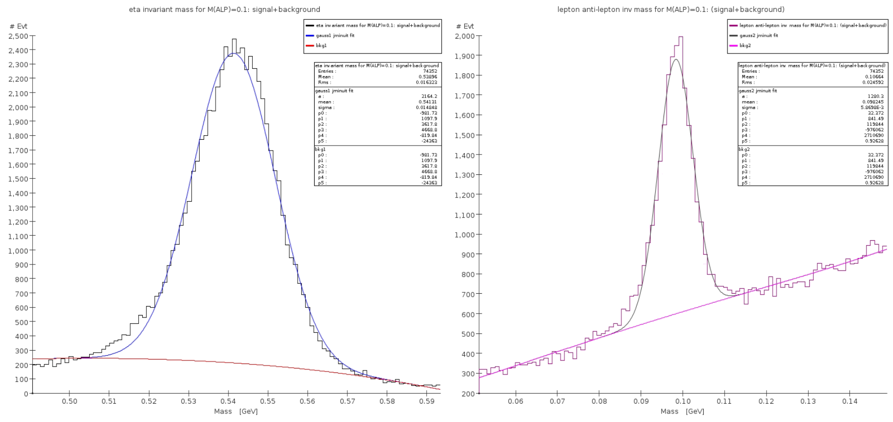
Figure 31: Invariant mass of $\gamma e^{+}e^{-}$ (left) and of the $e^{+}e^{-}$ system (right) for a vector boson with mass 100 MeV merged with the Urqmd generated background. See text for an explanation of the fitting procedure.

The resulting values are shown in Fig. 32. The error bars are statistical only. The effect of the cuts applied to reduce the background from photon conversion is clearly visible, as they degrade the sensitivity for lower values of the $e^{+}e^{-}$ invariant mass.

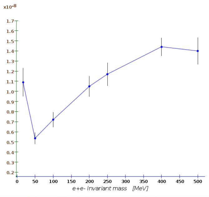
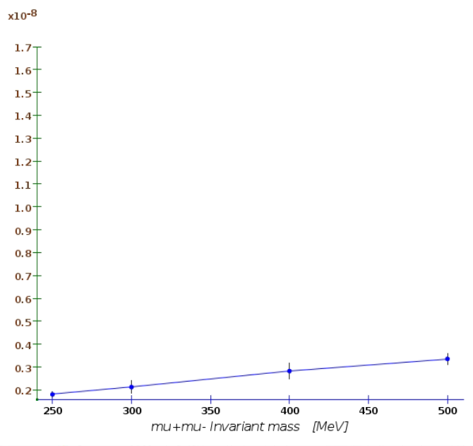
Figure 32: Branching ratio sensitivity for the process $\eta\rightarrow\gamma A^{\prime}\;;\;A^{\prime}\rightarrow e^{+}e^{-}$(left) and $\eta\rightarrow\gamma A^{\prime}\;;\;A^{\prime}\rightarrow\mu^{+}\mu^{-}$ (right) as a function of the mass of the vector boson $A^{\prime}$.

IX.2 $A^{\prime}\rightarrow e^{+}e^{-}$: Detached-vertex analysis

This study aimed at evaluating the sensitivity of the detector to events with a long-lived particle decaying into a lepton pair and a secondary vertex detached from the $\eta$ production vertex. Since no Standard Model process is known to be responsible for a similar event topology, the rejection of the background with the $detached-vertex$ analysis is expected to improve considerably compared to the $bump-hunt$ analysis. The vector boson $A^{\prime}$ was generated within a mass range between 17 MeV and 500 MeV. For each value of mass, $c\tau$ of the vector boson was varied from 20 mm to 150 mm. A total of 28 event sets were generated and fully reconstructed. The analysis of the kinematics follows the same guidelines as for the $bump-hunt$ analysis. Additional cuts on the $\chi^{2}$ from the fit of two charged tracks to a common vertex and on the distance between the primary and secondary vertexes were applied. The goal of those cuts was to remove events with particles originating from the $\eta$ production point. Since the $\beta\gamma$ boost of the $A^{\prime}$ depends on its mass, the cuts above were optimized for each individual event set.

The final reconstruction efficiency for this process, including the additional vertex cuts, was found to be between $\sim$2% and $\sim$10% for the signal samples and of order $\mathcal{O}(10^{-10})$ for the Urqmd background. The resulting branching ratio sensitivity is shown in Fig. 33, as a function of the invariant mass of the vector boson. The error bars are statistical only. Even for the detached-vertex analysis, the lower $e^{+}e^{-}$ invariant mass region shows a lower sensitivity. This is a consequence of the larger $\beta\gamma$ factor of bosons with lighter masses, which boosts the secondary vertex toward the outermost region of the detector. When that happens, the detector records fewer hits, which is detrimental to the reconstruction efficiency. The kinematic cut aiming at removing converting photons also worsens the sensitivity. The poorer reconstruction efficiency is reflected in a lower branching ratio sensitivity in the low-mass region, which ranges between $5.5\times 10^{-9}$ to $2.4\times 10^{-8}$. For the remaining mass regions the branching ratio sensitivity is of order $1\times 10^{-10}$.

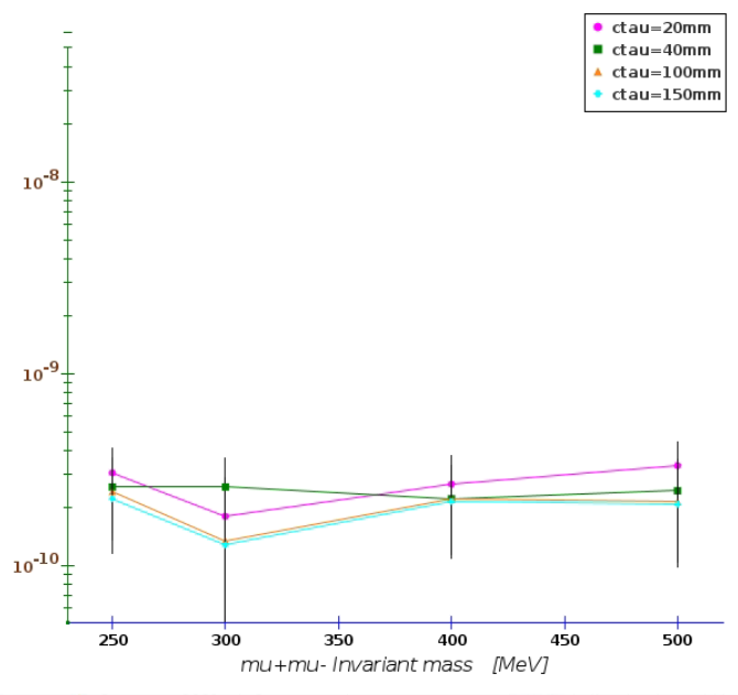
Figure 33: Branching ratio sensitivity for the process $\eta\rightarrow\gamma A^{\prime}\;;\;A^{\prime}\rightarrow e^{+}e^{-}$ (left) and $\eta\rightarrow\gamma A^{\prime}\;;\;A^{\prime}\rightarrow\mu^{+}\mu^{-}$ (right) as a function of the mass and $c\tau$ of the a long-lived vector boson $A^{\prime}$.

IX.3 $A^{\prime}\rightarrow\mu^{+}\mu^{-}$: Bump-hunt analysis

The rationale for studying this decay mode is because it probes the lepton flavor dependence of the $A^{\prime}$ vector. If coupling of the $A^{\prime}$ was different for electrons and muons that could explain some anomalies recently observed, in particular that related to the measurement of muon $g-2$. Furthermore, we expect for this final state a reduced contribution to the background from converting photons: $\gamma\rightarrow e^{+}e^{-}$ and from $\pi^{0}$ decays, and, consequently, a higher branching ratio sensitivity. Four event sets were generated in a mass ranging between 250 and 500 MeV. The largest background to this channel was found to originate from mis-identified pions, mistakenly reconstructed as muons. The $\pi$/$\mu$ mis-identification probability for the detector configuration considered here, has a conservative value of $\simeq$ 3.5% (or, $\sim$0.12% for mis-identifying both leptons). Since the probability of generating two charged pions in the primary interaction interaction is almost 11% (see, also, Fig. 17), and the probability of having at least one $\pi^{0}$ is 58%, we expect that about $\sim 1.9\times 10^{11}$ events could potentially fake a $\eta\rightarrow\gamma\mu^{+}\mu^{-}$ final state.

The full chain of generation-simulation-reconstruction-analysis was repeated for each event set. Very generic requirements on the quality of reconstructed particles were applied to signal and background. Neutral pions, decaying into $\gamma e^{+}e^{-}$ and $\gamma\gamma$, where reconstructed by considering all combinations of photons, electrons and positrons with an invariant mass within 5 MeV from $\pi^{0}$ mass. Finally, the events were required to have a topology consistent with a $\gamma\mu^{+}\mu^{-}$ final state, and an invariant mass compatible with the $\eta$ mass. The largest background was found for values of the $\mu^{+}\mu^{-}$ invariant mass corresponding to the middle of the kinematically allowed range. The final reconstruction efficiency for this process was found to be between $\sim$16% and $\sim$42% for the signal samples and of order $\mathcal{O}(10^{-8})$ for the Urqmd background. For illustrative purposes of the detector performance, Fig. 34 shows the invariant mass distribution of the reconstructed $\gamma\mu^{+}\mu^{-}$ and di-lepton system for the signal and the Urqmd background, assuming a BR($\eta\rightarrow\gamma A^{\prime}$)= $9\times 10^{-6}$ and an $\eta$ sample of $5.4\times 10^{9}$ events (corresponding to $\sim 4.9\times 10^{-5}$ of the full integrated luminosity). The distribution was fitted using the sum of a Gaussian distribution and a 5th-order polynomial. The branching ratio sensitivity for this process was calculated according to Eqs. 102-104.

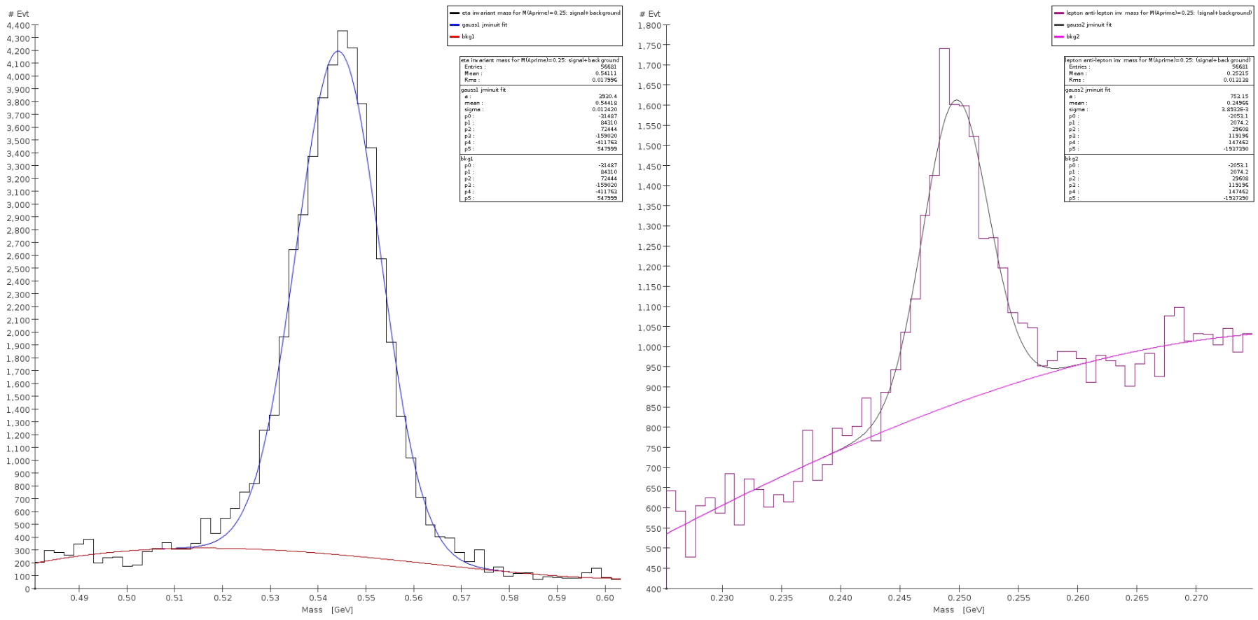
Figure 34: Invariant mass of $\gamma\mu^{+}\mu^{-}$ (left) and of the $\mu^{+}\mu^{-}$ system (right) for a vector with mass 250 MeV. The plot includes the Urqmd generated background. See text for an explanation of the fitting procedure.

The resulting branching ratio sensitivity is summarized in the right plot of Fig. 32, as a function of the invariant mass of the short-lived vector boson. The best sensitivity is observed near the lower kinematic limit of the $\mu^{+}\mu^{-}$ invariant mass, where the feed trough from background is approximately half of that observed in the central region.

IX.4 $A^{\prime}\rightarrow\mu^{+}\mu^{-}$: Detached-vertex analysis

The study for this channel was carried for masses of the vector boson in the range between 250 MeV and 500 MeV. For each value of the mass, the $c\tau$ of the resonance was varied from 20 mm to 150 mm. A total of 16 event sets were generated and fully reconstructed. This analysis follows the same guidelines of the $bump-hunt$ analysis. Additional cuts on the $\chi^{2}$ from the fit of two charged tracks to a common vertex and on the distance between the primary and secondary vertexes were applied. The goal of those cuts was to remove events with particles originating from the $\eta$ production point. Since the $\beta\gamma$ boost of the $A^{\prime}$ depends on its mass, the cuts above were optimized for each individual event set.

The final reconstruction efficiency for this process was found to be between $\sim$6% and $\sim$24% for the signal and of order $\mathcal{O}(10^{-11})$ for the Urqmd background. The resulting branching ratio sensitivity is shown in the right plot of Fig. 33, as a function of the invariant mass and of $c\tau$ of the a long-lived of the vector boson. The $\beta\gamma$ boost for $\mu^{+}\mu^{-}$ invariant masses close to the lower limit of the kinematically allowed range is larger and the secondary vertex occurs in the outermost region of the detector. For such events fewer hits are recorded by the tracking detectors. Nonetheless, the branching ratio sensitivity is mostly uniform in the $\mu^{+}\mu^{-}$ invariant mass range considered in this study.

IX.5 $B\rightarrow\pi^{+}\pi^{-}$: Bump-hunt analysis

In some theoretical models the coupling of the vector boson to leptons is suppressed, as it occurs, for example with the “Leptophobic B boson model”. In those cases, the preferred decay mode of the vector boson is into pions or photon pairs. Therefore, in addition to the leptonic decay modes, we have considered also the decay mode of a vector boson (in this case, often referred to as “B boson”), into a pair of charged pions. From the experimental point of view, analogously to the $A^{\prime}\rightarrow\mu^{+}\mu^{-}$ decay, this channel has a reduced background contribution from converting photons $\gamma\rightarrow e^{+}e^{-}$ and from $\pi^{0}$ decay. On the other side, the Standard Model background is expected to be particularly challenging, due to the large yield of two-pion events from nuclear scattering of the beam onto the target, accompanied by one or more photons from $\pi^{0}$ and $\eta$ decays.

The reconstruction of this process is further complicated by the fact that the detector configuration adopted for these studies, along with the algorithms implemented in the trigger systems, are optimized for the detection of leptons and for the rejection of hadrons. Consequently, we expect a somehow lower sensitivity compared to the other channels. Besides the combinatorics background, the relatively large branching ratios of the $\eta\rightarrow\pi^{+}\pi^{-}\pi^{0}$ and $\eta\rightarrow\pi^{+}\pi^{-}\gamma$, represents an irreducible, non-resonant background to searches of New Physics with bump-hunt techniques.

The study for this final state was carried for masses of the B boson ranging between 300 MeV and 500 MeV. Each sample consists of $3.5\times 10^{5}$ $\eta\rightarrow\gamma B\;;\;B\rightarrow\pi^{+}\pi^{-}$ events. The full chain of generation-simulation-reconstruction-analysis was repeated for each event set. Very generic requirements on the quality of reconstructed particles were applied to the signal and background samples. We found, as expected, that the largest background is due to purely combinatorics hadronic events (namely, events without $\eta$ mesons) containing two pions (cf. Fig.22) and one photon. The background was larger for values of $M(B)$ where the invariant mass of the $\pi^{+}\pi^{-}$ pair is in the lower and central region of the kinematically allowed range. In this region, in fact, the combinatoric background mimics more closely the kinematics of the $\eta\rightarrow\gamma B\;;\;B\rightarrow\pi^{+}\pi^{-}$ process. Neutral pions, decaying into $\gamma e^{+}e^{-}$ and $\gamma\gamma$, were reconstructed by considering all combinations of photons, electrons and positrons with an invariant mass within 5 MeV from $\pi^{0}$ mass, and removed from the event. Finally, the reconstructed particles were required to have a topology consistent with a $\gamma\pi^{+}\pi^{-}$ final state, and an invariant mass compatible with the $\eta$ mass.

The total reconstruction efficiency for this process was found equal to $\sim$2% for the signal samples and of order $\mathcal{O}(10^{-7})$ for the Urqmd background. For illustrative purposes, Fig. 35 shows the invariant mass distribution of the reconstructed $\gamma\pi^{+}\pi^{-}$ and $\pi^{+}\pi^{-}$ system for the signal and the Urqmd background, assuming a BR($\eta\rightarrow\gamma B$)= $5\times 10^{-2}$ and an $\eta$ sample of $5.4\times 10^{9}$ events (corresponding to $\sim 4.9\times 10^{-5}$ of the full integrated luminosity). The distribution was fitted using the sum of a Gaussian and a 5th-order polynomial. The branching ratio sensitivity for this process was calculated according to Eqs. 102-104.

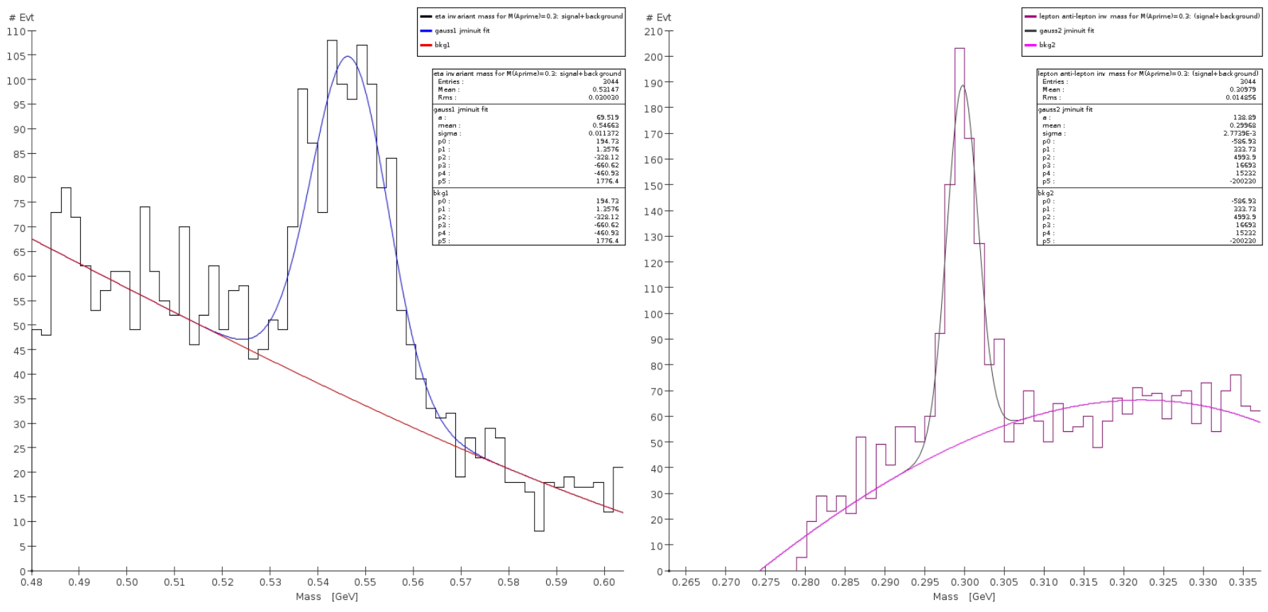
Figure 35: Invariant mass of $\gamma\pi^{+}\pi^{-}$ (left) and of the $\pi^{+}\pi^{-}$ system (right) for a vector boson with mass 300 MeV. The plot includes the Urqmd generated background. See text for an explanation of the fitting procedure.

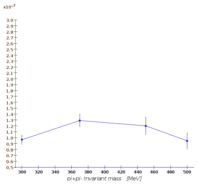
Figure 36: Branching ratio sensitivity for the process $\eta\rightarrow\gamma B\;;\;B\rightarrow\pi^{+}\pi^{-}$ with the bump-hunt analysis as a function of the mass of the vector boson $B$.

The resulting branching ratio sensitivity is summarized in Fig. 36. The error bars are statistical only. The best sensitivity is observed near the upper and lower kinematic limits of the $\pi^{+}\pi^{-}$ invariant mass, where the feed trough from background is approximately 30%-40% lower than that observed in the central region.

IX.6 $B\rightarrow\pi^{+}\pi^{-}$: Detached-vertex analysis

The study for this final state was carried for vector masses in the range between 300 MeV and 500 MeV. For each value of mass, the $c\tau$ of the resonance was varied from 20 mm to 150 mm. A total of 16 event sets were generated and fully reconstructed. The analysis for the kinematic variables follows the same guidelines of the $bump-hunt$ analysis. A further cut on the $\chi^{2}$ of vertex fit and on the distance between the primary and secondary vertexes were applied in order to remove events with particles originating from the $\eta$ production point. Since the $\beta\gamma$ boost of the $B$ boson depends on its mass, those cuts were optimized for each individual event set.

The final reconstruction efficiency for this process with the additional vertex cuts was found to be between $\sim$1% and $\sim$1.5% for the signal samples and of order $\mathcal{O}(10^{-9})$ for the Urqmd background. The $\beta\gamma$ boost for $\mu^{+}\mu^{-}$ invariant masses closer to the lower limit of the kinematically allowed range is larger and the secondary vertex occurs in the outermost region of the detector, with fewer hits in both tracking detectors. Nonetheless, the branching ratio sensitivity is mostly uniform in the $\pi^{+}\pi^{-}$ invariant mass range considered in this study.

IX.7 Sensitivity to selected theoretical models

In this section we consider four distinct theoretical models, discussed in details in Sec. III, for which New Physics appears through the vector portal. More specifically, the branching ratio sensitivity obtained in the previous sections is used to determine the sensitivity to the corresponding coupling constants.

IX.7.1 Minimal Dark Photon Model

The relevant parameter of this model is the kinetic mixing $\epsilon^{2}$ defined in Sec. 26. The master formula for $Br(\epsilon^{2})$ (cf. Eq. (105)) was obtained from Ref. Batell et al.:

$$BR_{\eta\rightarrow\gamma A^{\prime}}=BR_{\eta\rightarrow\gamma\gamma}\times 2\epsilon^{2}\left(1-\frac{m_{A^{\prime}}^{2}}{m_{\eta}^{2}}\right)$$ (106)

The partial widths of the A’ into leptons are Ilten et al. (2016):

$$\Gamma_{A^{\prime}\rightarrow\ell^{+}\ell^{-}}=\epsilon^{2}\alpha_{EM}\frac{m_{A^{\prime}}}{3}\left(1+2\nicefrac{{m_{l}^{2}}}{{m_{A^{\prime}}^{2}}}\right)\sqrt{1-4\nicefrac{{m_{l}^{2}}}{{m_{A^{\prime}}^{2}}}}$$ (107)

where $\ell=e,\mu,\tau.$ and $m_{A^{\prime}}>2m_{\ell}$. The total width can be expressed as:

$$\Gamma_{A^{\prime}}=\sum_{\ell}\Gamma_{A^{\prime}\rightarrow\ell^{+}\ell^{-}}+\Gamma_{A^{\prime}\rightarrow hadrons}+\Gamma_{A^{\prime}\rightarrow invisible}.$$ (108)

Following Ref. Ilten et al. (2016), for this work, we assume that:

$$\Gamma_{A^{\prime}\rightarrow hadrons}=\Gamma_{A^{\prime}\rightarrow\mu^{+}\mu^{-}}\Re_{\mu}(A^{\prime}),\qquad\Gamma_{A^{\prime}\rightarrow invisible}=0$$

where $\Re_{\mu}(A^{\prime})=\nicefrac{{\sigma_{e^{+}e^{-}\rightarrow hadrons}}}{{\sigma_{e^{+}e^{-}\rightarrow\mu^{+}\mu^{-}}}}$  Zyla et al. (2020a). A consequence of Eqs. (107) and 108 is that the value of $\epsilon^{2}$ and the lifetime of the $A^{\prime}$ are directly interconnected. Therefore, in a detached-vertex analysis the region of $\epsilon^{2}$ which could be explored is bound from above by the size of the fiducial volume where the secondary vertex of the dark photon is being reconstructed. For this work, we have conservatively used a fiducial volume consisting in a sphere with radius equal to 1 cm.

Inserting in Eqs. 106-108, the values of the branching ratio sensitivity obtained for each value of the $A^{\prime}$ mass and $c\tau$ considered in this study, we show the plot for the corresponding sensitivity of $\varepsilon^{2}$ in in Fig. 37 for the $bump-hunt$ and the detached-vertex analyses.

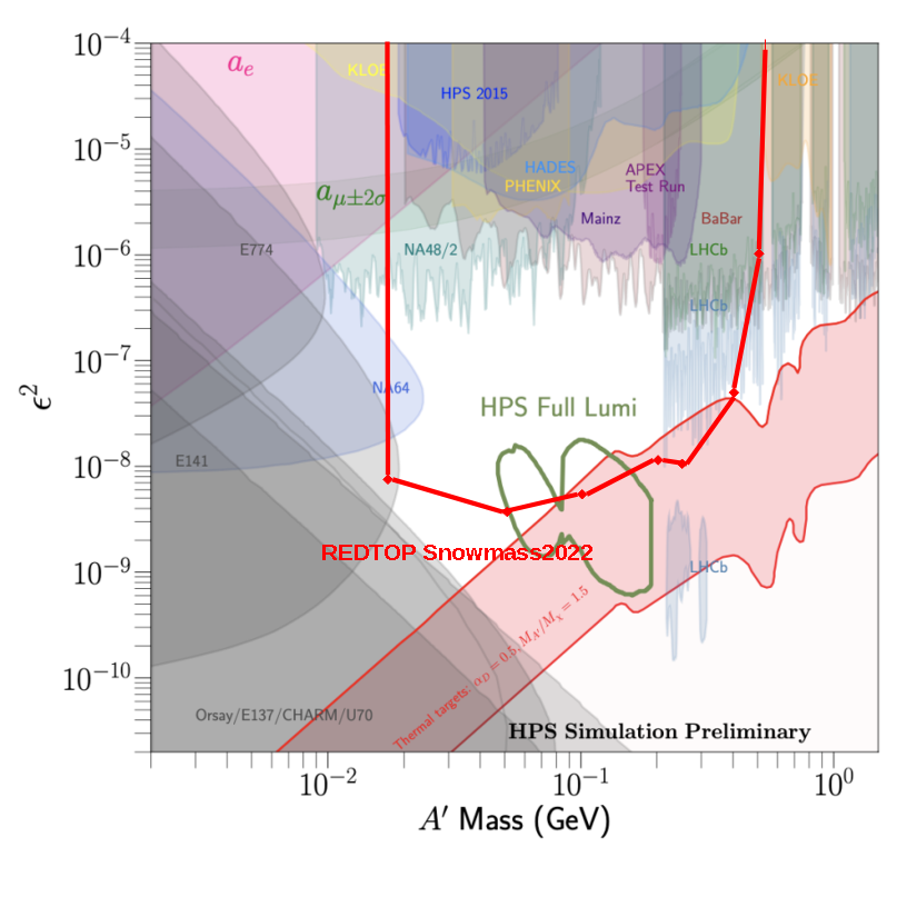
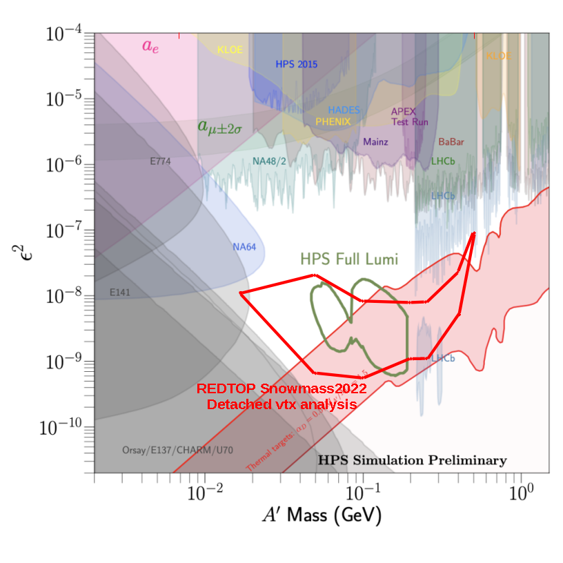
Figure 37: Sensitivity to to $\varepsilon{}^{2}$ for the processes $\eta\rightarrow\gamma A^{\prime}$ for integrated beam flux of $3.3\times 10^{18}$ POT. Left plot: bump-hunt analysis. Right plot: detached-vertex analysis).

IX.7.2 Leptophobic B boson Model

In this section we place limits on the $B$ boson parameters. Let us first consider the $\eta^{(\prime)}\to\pi^{0}\gamma\gamma$ and $\eta^{\prime}\to\eta\gamma\gamma$ decay channels. On the experimental side, the CrystalBall collaboration at AGS in 2008 Prakhov et al. (2008) and the A2 collaboration at the Mainzer Microtron (MAMI) in 2014 Nefkens et al. (2014) published the first measurements of the diphoton energy spectrum $d\Gamma(\eta\to\pi^{0}\gamma\gamma)/dm_{\gamma\gamma}^{2}$, along with the associated branching ratio (BR). They reported the measurements $\mbox{BR}=(2.21\pm 0.24\pm 0.47)\times 10^{-4}$ and $\mbox{BR}=(2.54\pm 0.27)\times 10^{-4}$, respectively, based on the analysis of $\sim 1.2\times 10^{3}$ $\eta\to\pi^{0}\gamma\gamma$ decay events. Surprisingly low in comparison with all previous measurements is the 2006 result reported by the KLOE collaboration Di Micco et al. (2006), $\mbox{BR}=(0.84\pm 0.27\pm 0.14)\times 10^{-4}$, based on a sample of only $68\pm 23$ events. Very recently, however, the KLOE collaboration has presented a new analysis, finding a preliminary value of $\mbox{BR}=(1.23\pm 0.14)\times 10^{-4}$ based on the analysis of $\sim 1.4\times 10^{3}$ $\eta\to\pi^{0}\gamma\gamma$ events Cao (2022). For the $\eta^{\prime}\to\pi^{0}\gamma\gamma$ decay, the BESIII collaboration recently reported for the first time the $m_{\gamma\gamma}^{2}$ invariant mass distribution Ablikim et al. (2017b) and the measured branching fraction, $\mbox{BR}=(3.20\pm 0.07\pm 0.23)\times 10^{-3}$. Finally, for the $\eta^{\prime}\to\eta\gamma\gamma$ decay, a measurement of $\mbox{BR}<1.33\times 10^{-4}$ at 90% CL has been provided, again for the first time, by the BESIII collaboration Ablikim et al. (2019). This experimental information is important to place limits on the $B$ boson parameters.

On the theoretical side, the $B$ boson exchange contribution to the amplitude of these decays, defined in Eq. (11), depends on three parameters: the baryonic fine structure constant, $\alpha_{B}$, and the $B$ boson resonance parameters, mass and width, $m_{B}$ and $\Gamma_{B}$. Adding this to the Standard Model contribution Escribano et al. (2020), along with the available experimental data, allows us to place limits on the $B$ boson parameters Escribano et al. (2022b). These limits are shown in Fig. 38 in terms of $\alpha_{B}$ and $m_{B}$. In this figure, we require the amplitude not to exceed the corresponding branching ratios at $2\sigma$, and fixed the $B$ boson width to the decay width of the $\omega$ meson for illustration purposes. These results differ somewhat from Tulin (2014), which assumed no contribution from the Standard Model and the narrow width approximation, i.e., $\mbox{BR}(\eta\to\pi^{0}\gamma\gamma)=\mbox{BR}(\eta\to B\gamma)\times\mbox{BR}(B\to\pi^{0}\gamma)$, with $\mbox{BR}(B\to\pi^{0}\gamma)=1$.

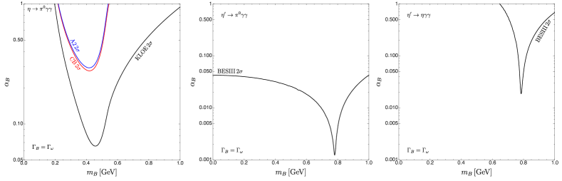
Figure 38: Limits on the leptophobic $B$ boson mass $m_{B}$ and coupling $\alpha_{B}$ from $\eta\to\pi^{0}\gamma\gamma$ (left), $\eta^{\prime}\to\pi^{0}\gamma\gamma$ (middle) and $\eta^{\prime}\to\eta\gamma\gamma$ (right).

We next consider $B$ boson contributions to the decay $\eta\to\pi^{+}\pi^{-}\gamma$. The relevant parameter of this model is the couplings $\alpha_{B}$ defined above. The master formula for $Br(\alpha_{B})$ was obtained by numerically integrating Eq. (14) over the Mandelstam variable $t$. For simplicity, we have fixed the $B$ boson width to the width of the $\omega$ meson.

Inserting in the master formula the values of the branching ratio sensitivity obtained for each value of the $B$ mass considered, we obtain the corresponding sensitivity to $\alpha_{B}$. This is summarized in Fig. 39 for the $bump-hunt$ analysis only, since the leptophobic $B$ boson is predicted to have a short lifetime.

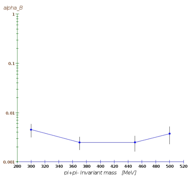
Figure 39: Sensitivity to $\alpha_{B}$ for the processes $\eta\rightarrow\gamma B\;;\;B\rightarrow\pi^{+}\pi^{-}$ for the bump-hunt analysis as a function of the mass of the short-lived $B$ boson.

IX.7.3 Protophobic Fifth Force Model

The relevant parameter of this model is the $\varepsilon_{n}^{2}$ defined in Eqs. (18) and (19); . For simplicity, we will set $\varepsilon_{s}\equiv 0$, but we remind the reader that this can have a sizeable impact on the branching ratio (cf. Fig. (3)). The branching ratios become:

$$\left(\dfrac{BR_{\eta\to\gamma X}}{BR_{\eta\to\gamma\gamma}}\right)_{\text{ABJ}}=\dfrac{8\varepsilon_{n}^{2}}{\pi\alpha}\left(1-\dfrac{m_{X}^{2}}{m_{\eta}^{2}}\right)^{3}\left[\dfrac{c_{\theta}-\sqrt{2}s_{\theta}}{c_{\theta}-2\sqrt{2}s_{\theta}}\right]^{2},$$ (109)

$$\left(\dfrac{BR_{\eta\to\gamma X}}{BR_{\eta\to\gamma\gamma}}\right)_{\text{VMD}}=\dfrac{\varepsilon_{n}^{2}}{8\pi\alpha}\left(1-\dfrac{m_{X}^{2}}{m_{\eta}^{2}}\right)^{3}\left[\dfrac{c_{\theta}-\sqrt{2}s_{\theta}}{c_{\theta}-2\sqrt{2}s_{\theta}}\right]^{2}\left|9F_{\rho}(m_{X}^{2})-F_{\omega}(m_{X}^{2})\right|^{2}$$ (110)

These expressions are nearly identical (at the $\sim 3-4\%$ level) for $m_{X}\ll m_{\rho},\,m_{\omega}$, but the branching ratio in the ABJ scheme is smaller by a factor of $\sim 2-3$ near threshold, where the form factors become important. Inserting in Eq. (109) and 110 the values of the branching ratio sensitivity obtained for the point at 17 MeV in the analyses above, we derive the sensitivity for the parameter $\varepsilon_{n}^{2}$. The values obtained for the two model considered in this discussion are summarized in Table 24.

Scheme	$\varepsilon_{n}^{2}$
	Sensitivity
$ABJ$	$1.41\pm 0.17\times 10^{-10}$
VMD	$1.46\pm 0.17\times 10^{-10}$

Table 24: Sensitivity to $\varepsilon_{n}$ for a 17-MeV protophobic gauge boson model in the ABJ and VMD schemes. We assume that $X$ decays to neutrinos contribute negligibly to its total width, i.e, that $BR(X\to e^{+}e^{-})\approx 1$; the sensitivity scales as the inverse of the decay branching ratio for this channel.

X Sensitivity to the Scalar portal

The Scalar portal can be probed via decays of the $\eta$-meson with a $\pi^{0}$ meson in the final state. Three processes have been considered for these studies:

• $p+Li\rightarrow\eta+X\;with\;\eta\rightarrow\pi^{0}H\;and\;h\rightarrow e^{+}e^{-}$

• $p+Li\rightarrow\eta+X\;with\;\eta\rightarrow\pi^{0}H\;and\;h\rightarrow\mu^{+}\mu^{-}$

• $p+Li\rightarrow\eta+X\;with\;\eta\rightarrow\pi^{0}H\;and\;h\rightarrow\pi^{+}\pi^{-}$

As for the case of the Vector portal, a bump-hunt and a detached-vertex analysis were performed to test the performance of different components of the detector.

X.1 $h\rightarrow e^{+}e^{-}$: $Bump-hunt$ analysis

This study aims at evaluating the sensitivity of the detector in the assumption that scalar boson has a decay length not resolvable by the tracking system. In this case, the process is identified exclusively through its kinematics, in particular by observing a bump in the invariant mass of the $\ell\bar{\ell}$ or the $\pi^{+}\pi^{-}$ system.

The scalar boson h was generated with a mass ranging between 17 MeV and 400 MeV. The h was decayed promptly within GenieHad, by setting the vertex of the di-lepton in the point where the proton struck the target. This final state has a large contribution from background on the lower side of the kinematically allowed mass range. The process responsible for that is the decay $\eta\rightarrow\gamma\gamma$, when one of the photons converts into a $e^{+}e^{-}$ pair and an extra accidental or misidentified $\pi^{0}$ is found in the event, with kinematics compatible with the $\eta$ mass. Another large contribution to the background originates from the decay of the $\eta$ meson: $\eta\rightarrow\gamma e^{+}e^{-}$, when the radiative photon is paired to another photon to fake a $\pi^{0}$ and the kinematics of the event is compatible with a di-lepton mass near the $h$ mass.

The full chain of generation-simulation-reconstruction-analysis was repeated for each event set. The information from TOF and PID systems contributes in reducing the background by a factor $\mathcal{\sim}10{}^{4})$. Very generic requirements on the quality of reconstructed particles were applied to the signal and background samples. No cuts were applied to the reconstructed $e^{+}e^{-}$ vertex. Neutral pions, decaying into $\gamma e^{+}e^{-}$ and $\gamma\gamma$, where reconstructed by considering all combinations of photons, electrons and positrons with an invariant mass within 5 MeV from $\pi^{0}$ mass. This requirement is able to reject most of the combinatoric background with no $\eta$ mesons in the final state. Similarly, photons converting into a $e^{+}e^{-}$ pair where reconstructed by requiring that the invariant mass of the $e^{+}e^{-}$ system was lower than 5 MeV.

The total reconstruction efficiencies for this process was found to be between 6% and 16% for the signal and in the range $10^{-9}-10^{-8}$ for the Urqmd background. For illustrative purposes, Fig. 40 shows the invariant mass distribution of the reconstructed $\pi^{0}e^{+}e^{-}$ and di-lepton system for the signal and the Urqmd background, assuming BR($\eta\rightarrow\pi^{0}H$)= $2.5\times 10^{-4}$ and an $\eta$ sample of $2\times 10^{8}$ (corresponding to $1.8\times 10^{-6}$ of the full integrated luminosity). The distribution was fitted using the sum of a Gaussian and a 5th-order polynomial. The branching ratio sensitivity for this process was calculated according to Eqs. 102-104. It is summarized in Fig. 41, as a function of the invariant mass of the scalar boson.

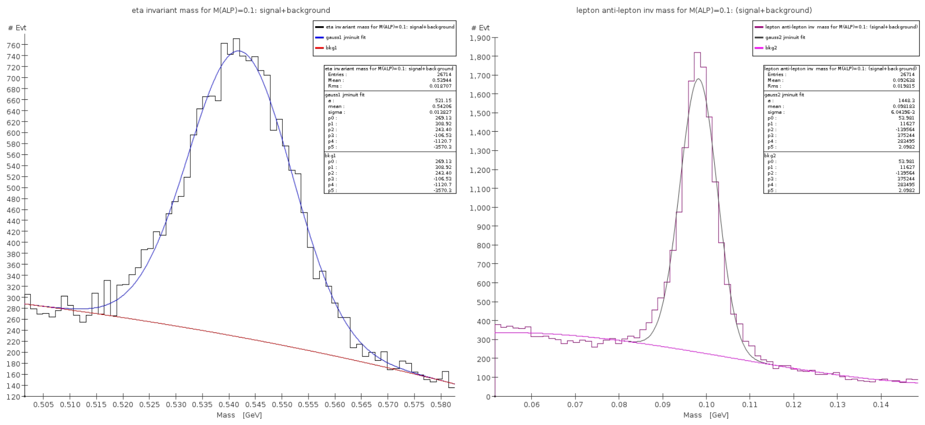
Figure 40: Invariant mass of $\pi^{0}e^{+}e^{-}$ (left) and of the $e^{+}e^{-}$ system (right) for a scalar with mass 100 MeV. The plot includes the Urqmd generated background. See text for an explanation of the fitting procedure.

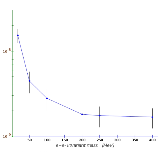
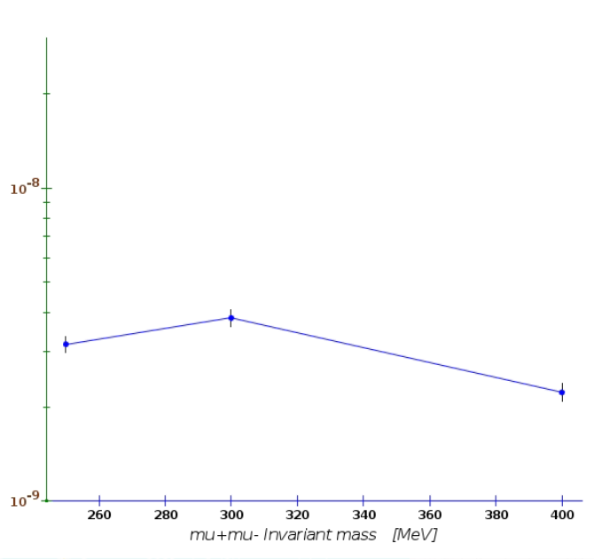
Figure 41: Branching ratio sensitivity for the process $\eta\rightarrow\pi^{0}h\;;\;h\rightarrow e^{+}e^{-}$ (left) and $\eta\rightarrow\pi^{0}h\;;\;h\rightarrow\mu^{+}\mu^{-}$ (right) as a function of the mass of the scalar boson $h$.

X.2 $h\rightarrow e^{+}e^{-}$: Detached-vertex analysis

This study aims at evaluating the sensitivity of the detector to $\eta$ mesons decaying into long-lived particles, further decaying into a $\mu^{+}\mu^{-}$ pair with a secondary vertex detached from the $\eta$ production point. As noted previously, no Standard Model process is known to be responsible for a similar event topology. Consequently, we expected that the rejection of the background would improve considerably compared to a bump-hunt analysis. The scalar h was generated within a mass range between 17 MeV and 400 MeV. For each value of the mass, $c\tau$ of the resonance was varied from 20 mm to 150 mm. A total of 24 event sets were generated and fully reconstructed.The analysis of the kinematics follows the same guidelines as for the $bump-hunt$ analysis. Additional cuts on the $\chi^{2}$ from the fit of two charged tracks to a common vertex and on the distance between the primary and secondary vertexes were applied. The goal of those cuts was to remove events with particles originating from the $\eta$ production point. Since the $\beta\gamma$ boost of the $A^{\prime}$ depends on its mass, the cuts above were optimized for each individual event set.

The total reconstruction efficiency for this process, including the additional vertex cuts, was found to be between $\sim$1\% and $\sim$9\% for the signal samples and of order $\mathcal{O}(10^{-10})$ for the Urqmd background. The lower reconstruction sensitivity is due to the extra cuts on detached vertex. The resulting branching ratio sensitivity curve is shown in Fig. 42, as a function of the invariant mass and $c\tau$ of the long-lived scalar boson. The lower $e^{+}e^{-}$ invariant mass region shows a degraded sensitivity. This is a consequence of the larger $\beta\gamma$ factor, boosting the secondary vertex toward the outermost region of the detector, were the reconstruction efficiency is lower. The kinematic cut that removes converting photons also degrades the sensitivity. The lower reconstruction efficiency is reflected in a lower branching ratio sensitivity in the low-mass region, the former being of order $\mathcal{O}(10^{-8})$. For the remaining mass region, the branching ratio sensitivity is close to $1\times 10^{-9}$

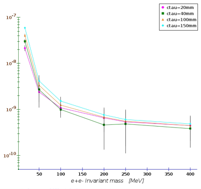
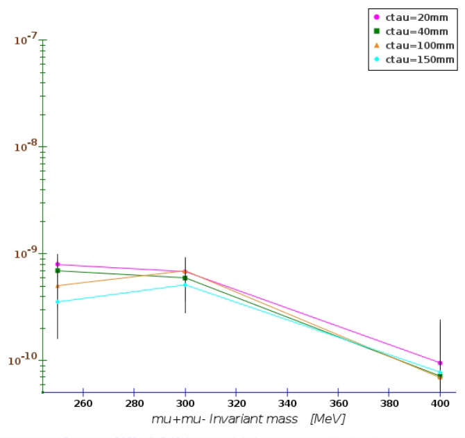
Figure 42: Branching ratio sensitivity for the process $\eta\rightarrow\pi^{0}h\;and\;h\rightarrow e^{+}e^{-}$ (left) and $\eta\rightarrow\pi^{0}h\;;\;h\rightarrow\mu^{+}\mu^{-}$ (right) as a function of the mass and $c\tau$ of a long-lived scalar boson $h$.

X.3 $h\rightarrow\mu^{+}\mu^{-}$: Bump-hunt analysis

As already observed for the Vector portal case, the study of this decay mode gives the opportunity to probe lepton universality and to explore a complementary, and possibly, reduced, background source. We expect for this final state a reduced background contribution from converting photons $\gamma\rightarrow e^{+}e^{-}$ and from $\pi^{0}$ decays, and, possibly, a higher branching ratio sensitivity. Four event sets were generated with the $h$ mass ranging between 250 MeV and 500 MeV. The largest background contribution to this final state was found to originate from mis-identified pions, mistakenly reconstructed as muons. The $\pi$/$\mu$ mis-identification probability for the detector layout considered in this work has a conservative value of $\simeq$ 3.5% (or, $\simeq$ 0.12% for mis-identifying both leptons). Since the probability of generating two charged pions in the primary interaction is almost 11% (see, also, Fig. 17), and the probability of having at least one $\pi^{0}$ is 58%, we expect that about $\sim 1.9\times 10^{11}$ events could possibly fake a $\eta\rightarrow\pi^{0}\mu^{+}\mu^{-}$ process. The second largest background was due to the process: $\eta\rightarrow\gamma\mu^{+}\mu^{-}$, when either an accidental/misidentified photon is paired with the radiative photon, and they both fake a $\pi^{0}$.

The full chain of generation-simulation-reconstruction-analysis was repeated for each event set. Neutral pions, decaying into $\gamma e^{+}e^{-}$ and $\gamma\gamma$, where reconstructed by considering all combinations of photons, electrons and positrons with an invariant mass within 5 MeV from $\pi^{0}$ mass. Finally, the events were required to have a topology consistent with a $\pi^{0}\mu^{+}\mu^{-}$ final state, and an invariant mass compatible with the $\eta$ mass. The largest background was found for values of the $\mu^{+}\mu^{-}$ invariant mass values near the middle of the kinematically allowed range. The final reconstruction efficiency for this process was found to be between $\sim$14\% and $\sim$18\% for the signal and of order $\mathcal{O}(10^{-8})$ for the Urqmd background. For illustrative purposes, Fig. 43 shows the invariant mass distribution of the reconstructed $\pi^{0}\mu^{+}\mu^{-}$ and di-lepton system for the signal and the Urqmd background, assuming a BR($\eta\rightarrow\pi^{0}h$)= $5\times 10^{-5}$ and an $\eta$ sample of $2\times 10^{8}$ (corresponding to $\sim 1.8\times 10^{-6}$ of the full integrated luminosity). The distribution was fitted using the sum of a Gaussian and a 5th-order polynomial.

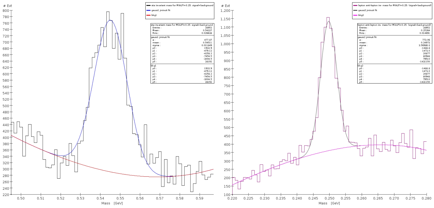
Figure 43: Invariant mass of $\pi^{0}\mu^{+}\mu^{-}$ (left) and of the $\mu^{+}\mu^{-}$ system (right) for a scalar boson $h$ with M($h$)=250 MeV. The plot includes the Urqmd generated background. See text for an explanation of the fitting procedure.

The branching ratio sensitivity estimated for this channel is shown in the right plot of Fig. 41, as a function of the invariant mass of the scalar boson. The highest sensitivity is observed near the upper kinematic limit of the $\mu^{+}\mu^{-}$ invariant mass, where the feed trough from combinatorics background is approximately half that observed in the central region.

X.4 $h\rightarrow\mu^{+}\mu^{-}$: Detached-vertex analysis

The study for this final state was carried for masses of the scalar boson in the range between 250 MeV and 400 MeV. For each value ofthe mass, the $c\tau$ of the resonance was varied from 20 mm to 150 mm. A total of 12 event sets were generated and fully reconstructed. The analysis for the kinematic variables follows the same guidelines of the $bump-hunt$ analysis. Further cuts on the $\chi^{2}$ of a fit to the secondary vertex and on the distance between the primary and secondary vertexes were applied. Since the $\beta\gamma$ boost of the particle depends on the mass of the boson $h$, the vertex cuts were individually optimized for each event set.

The final reconstruction efficiency for this analysis was found to be between $\sim$5\% and $\sim$10\% for the signal samples and of order $\mathcal{O}(10^{-10})$ for the Urqmd background. The resulting branching ratio sensitivity is shown in the right plot of Fig. 42, as a function of the invariant mass and of $c\tau$ of the long-lived scalar $h$. The $\beta\gamma$ boost for lower values of the $\mu^{+}\mu^{-}$ invariant mass is larger and the secondary vertex occurs in the outermost region of the detector, where the tracking systems has a lower reconstruction efficiency. That is reflected in a lower branching ratio sensitivity in the low-mass region of the kinematically allowed range.

X.5 $h\rightarrow\pi^{+}\pi^{-}$: $Bump-hunt$ analysis

The decay of the scalar boson h in non-leptonic mode is relevant for probing so called “hadrophilic” theoretical models, where the dark scalar or mediator couples more strongly to quarks rather than to leptons. For the present work, the detector layout and the algorithms implemented in the trigger, are optimized for the detection of final state containing leptons. Consequently, we expect a lower sensitivity compared to the other channels considered in this work. Furthermore, the relatively large branching ratio of the $\eta\rightarrow\pi^{+}\pi^{-}\pi^{0}$ process, represents an irreducible non-resonant background to searches of New Physics with bump-hunt techniques.

The study of this final state was carried for masses of the scalar $h$ in the range between 300 MeV and 400 MeV. Each sample consists of $2\times 10^{5}$ $\eta\rightarrow\pi^{0}h\;;\;h\rightarrow\pi^{+}\pi^{-}$ events. The largest background was found to originate from events containing three pions (cf. Fig.22). This background accounts for approximately 90% of the total. The remaining contribution was, in large part, originating from the three-body decay: $\eta\rightarrow\pi^{+}\pi^{-}\pi^{0}$, when one of the pions was mis-reconstructed or when an extra pion from the primary beam-target interaction was mistakenly associated to the decay of the $\eta$ meson. The background was larger for values of $M(h)$ where the invariant mass of the $\pi^{+}\pi^{-}$ system is in the central region of the kinematically allowed range, where the combinatoric background mentioned above mimics more closely the kinematics of the $\eta\rightarrow\pi^{0}h\;;\;h\rightarrow\pi^{+}\pi^{-}$ process.

The full chain of generation-simulation-reconstruction-analysis was repeated for each event set. Very generic requirements on the quality of reconstructed particles were applied to signal and background samples. Neutral pions, decaying into $\gamma e^{+}e^{-}$ and $\gamma\gamma$, where reconstructed by considering all combinations of photons, electrons and positrons with an invariant mass within 5 MeV from $\pi^{0}$ mass. Finally, the events were required to have a topology consistent with a $\gamma\mu^{+}\mu^{-}$ final state, and an invariant mass compatible with the $\eta$ mass.

The reconstruction efficiencies for this process was found to be between 1.5% and 2% for the $h$ signal and a relatively large $\sim 10^{-6}$ for the Urqmd background. For illustrative purposes, Fig. 44 shows the invariant mass distribution of the reconstructed $\pi^{0}\pi^{+}\pi^{-}$ and $\pi^{+}\pi^{-}$ systems for the signal and the Urqmd background, assuming a BR($\eta\rightarrow\pi^{0}h$) = $5\times 10^{-2}$ and an $\eta$ sample with $1\times 10^{7}$ events (corresponding to $0.9\times 10^{-7}$ of the full integrated luminosity). The distribution was fitted using the sum of a Gaussian and a 5th-order polynomial. As expected, the combinatoric background accumulated under the $\eta$ peak, is much worse than for any other channel examined.

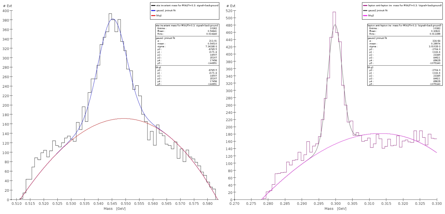
Figure 44: Invariant mass of $\pi^{0}\pi^{+}\pi^{-}$ (left) and of the $\pi^{+}\pi^{-}$ system (right) for a scalar boson $h$ with mass M($h$)=300 MeV. The plot includes the Urqmd generated background. See text for an explanation of the fitting procedure.

The branching ratio sensitivity for this process was, then, calculated according to Eqs. 102-104. The resulting sensitivity curve is shown in the left plot of Fig. 45, as a function of the invariant mass of the scalar $h$. Sensitivity is worse in the central region, as expected from the discussion above.

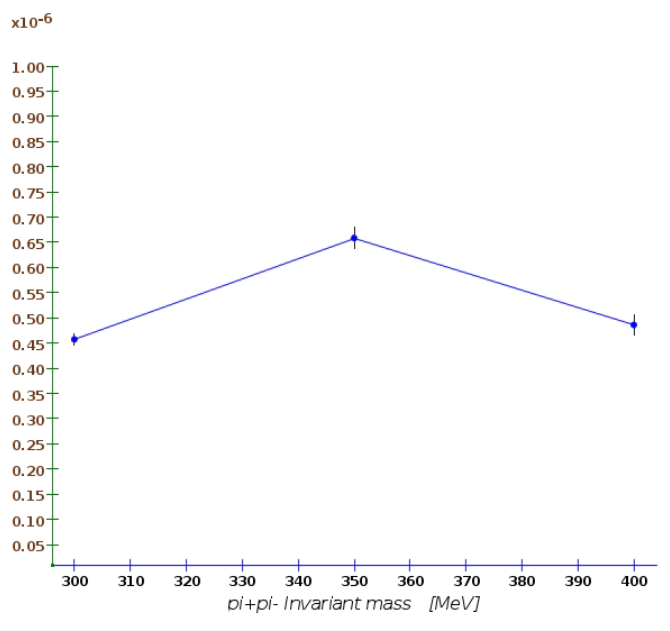
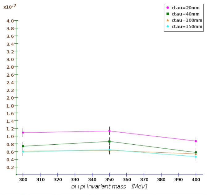
Figure 45: Branching ratio sensitivity for the process $\eta\rightarrow\pi^{0}h\;and\;h\rightarrow\pi^{+}\pi^{-}$ as a function of the mass of the scalar short-lived scalar $h$ (left) and of the mass and $c\tau$ of a long-lived scalar $h$.

X.6 $h\rightarrow\pi^{+}\pi^{-}$: Detached-vertex analysis

The experimental sensitivity to the $\eta\rightarrow\pi^{0}h\;withh\rightarrow\pi^{+}\pi^{-}$ channel improves considerably when the scalar boson travels inside the detector and it decays far from the interaction point. As already noted, the background from the Standard Model is dramatically reduced when constraints on a detached secondary vertex are imposed. The scalar $h$ was generated within a mass range between 300 MeV and 400 MeV. For each value of mass, the $c\tau$ of the resonance was varied from 20 mm to 15 0mm. A total of 12 event sets were generated and fully reconstructed. The analysis of the kinematics of the event follows the same guidelines of the $bump-hunt$ analysis. Further cuts on the $\chi^{2}$ of fit on the secondary vertex and on the distance between the primary and secondary vertexes were applied. Since the $\beta\gamma$ boost of the particle depends on the mass of the $h$, those cuts were optimized for each individual event set. A rejection factor of about $100\times$ was obtained for the background with respect to a purely kinematic analysis.

The final reconstruction efficiency for this process, including the additional vertex cuts, was found to range between $\sim$8\% and $\sim$15\% for the signal and of order $\mathcal{O}(10^{-8})$ for the Urqmd background. The resulting branching ratio sensitivity is shown in the right plot of Fig. 45, as a function of the invariant mass and of $c\tau$ of the long-lived scalar $h$. The effect of the vertex cuts, tuned to remove the combinatoric background, is clearly visible, with an improvement of the experimental sensitivity of almost one order of magnitude compared to the case of a short-lived scalar boson. We observe, once more, that the sensitivity is lower in the central region of the kinematically allowed mass range.

X.7 Sensitivity to selected theoretical models

In this section, we consider three distinct theoretical models, discussed in details in Sec. III, for which New Physics appears through the scalar portal. More specifically, the branching ratio sensitivity obtained in the previous sections is used to determine the sensitivity to the corresponding coupling constants.

X.7.1 Hadrophilic Scalar Mediator (including Spontaneous Flavor Violation models)

The $bump-hunt$ search in the $\pi^{0}(\pi^{+}\pi^{-})$ mode discussed in this section is directly applicable to the hadrophilic scalar mediator model described above in Section III.1.2; see Eq. (21). In this model, the scalar $S$ is produced via $\eta\rightarrow\pi^{0}S$ and subsequently decays via $S\rightarrow\pi^{+}\pi^{-}$. The scalar decays promptly in the parameter region of interest to REDTOP. Using the branching ratio formula for ${\rm Br}(\eta\rightarrow\pi^{0}S)$ given in Eq. (22), we can translate the limits presented in the left panel of Fig. 45 to limits in the mass-coupling $(m_{S}-g_{u})$ plane. The result is shown in Figure. 46 and in Figure. 4 (in the latter, superimposed on the parameter space explored by previous experiments). The sensitivity curve indicates that REDTOP will probe couplings of order $g_{u}\sim{\rm few}\times 10^{-6}$, extending the reach by a factor of a few beyond previous recasted bounds from the KLOE experiment Anastasi et al. (2016); Batell et al. (2019). Furthermore, it is worth highlighting that REDTOP nicely complements the sensitivity from proposed long-lived particle searches at FASER Kling and Trojanowski (2021), FASER2 Kling and Trojanowski (2021) and SHiP Batell et al. (2019), which will be able to explore longer lifetimes and smaller couplings.

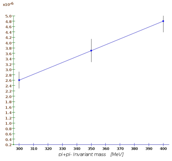
Figure 46: Sensitivity to $g_{u}$ for the process $\eta\rightarrow\pi^{0}h\;and\;h\rightarrow\pi^{+}\pi^{-}$ for the bump-hunt as a function of the mass of the short-lived scalar $S$.

X.7.2 Two-Higgs doublet model

The parameters $\lambda_{u}$ and $\lambda_{d}$ for this model, along with the branching ratios predicted for the decay channel $\eta^{(\prime)}\to\pi^{0}S$ are discussed in Sec. III.1.2. For the Two-Higgs doublet model considered in this work Abdallah et al. (2021), the branching ratio of $\eta\to\pi^{0}h^{\prime}$, in the assumption that $\lambda_{u}=\lambda_{d}$, is predicted to be $1.22\times 10^{-11}$, which is below REDTOP sensitivity in the present run. The situation is different for the case when $\lambda_{u}\neq\lambda_{d}$. It is known that the strange and non-strange isoscalar transition form factors are suppressed by $\epsilon\sim 0.012$. Therefore, the $\pi^{0}S$ production is dominated by the isovector form factor and the $\pi^{0}S$ production is proportional to $(\lambda_{u}-\lambda_{d})^{2}$. Thus, the branching ratio of $\eta\to\pi^{0}S$ approximately equals to:

$${\rm BR}(\eta\to\pi^{0}S)\simeq\frac{2}{3}B_{0}^{2}\frac{(\lambda_{u}-\lambda_{d})^{2}}{\Gamma_{\eta}^{{\rm tot}}}\frac{\sqrt{\tilde{E}_{\eta}^{2}-m_{\pi^{0}}^{2}}}{8\pi m_{\eta}^{2}},$$ (111)

where

$$\tilde{E}_{\eta}=\frac{m_{\eta}^{2}+m_{\pi^{0}}^{2}-m_{S}^{2}}{2m_{\eta}}.$$ (112)

In this model Abdallah et al. (2021), for non-zero difference of $(\lambda_{u}-\lambda_{d})^{2}$, BR$(\eta\to\pi^{0}h^{\prime})$ range is of order ${\cal O}(10^{-11}-10^{-5})$ with $m_{h^{\prime}}\simeq 17$ MeV. From the data presented in Fig. 42, we can conclude that REDTOP is sensitive to a slight mismatch in $\lambda_{u}$ and $\lambda_{d}$ values that keeps the LSND and MB fit intact.

Inserting the values obtained for each value of the $S$ mass into the formula for ${\rm BR}(\eta\to\pi^{0}S)$ in Eq. (111), the corresponding sensitivity for the parameter $(\lambda_{u}-\lambda_{d})^{2}$ is shown in Table 25 for the two analysis techniques we have used.

Process	$m_{S}$	Analysis	$(\lambda_{u}-\lambda_{d})^{2}$
			sensitivity
$\eta$$\rightarrow\pi^{0}S\;;\;S\rightarrow e^{+}e^{-}$	17 MeV	bump hunt	$2.0\times 10^{-13}$
$\eta$$\rightarrow\pi^{0}S\;;\;S\rightarrow\mu^{+}\mu^{-}$	17 MeV	detached vertex	$3.2\times 10^{-13}$

Table 25: Sensitivity to $(\lambda_{u}-\lambda_{d})^{2}$ for the process $\eta\to\pi^{0}S$ and $S\to e^{+}e^{-}$ and $S\to\mu^{+}\mu^{-}$.

X.7.3 Minimal scalar model

The theoretical aspects of Minimal Scalar model have been discussed in detail in Sec. III.1.2. The relevant parameter in this case is the mixing angle $\theta^{2}$ O’Connell et al. (2007b) between the Standard Model Higgs and its lighter counterpart. In this study we consider two parametrizations for the branching ratio, as they bring to numerically appreciable differences in the results.

Tulin parametrization

The master formula used for this parametrization of $Br(\vartheta^{2})$ is Tulin (2014):

$$BR_{\eta\rightarrow\pi^{0}h}\eqsim 1.8\times 10^{-6}\times\lambda^{\nicefrac{{1}}{{2}}}\left(1,\frac{M_{\pi_{0}}^{2}}{M_{\eta}^{2}},\frac{M_{H}^{2}}{M_{\eta}^{2}}\right)$$ (113)

where the function $\lambda$ has been defined in Sec. III.1.2. Inserting in Eq. (113) the values of the branching ratio sensitivity derived for each value of the $h$ mass, we obtain the corresponding plots of sensitivity for the parameter $\theta^{2}$. They are shown in Fig. 47 for the bump-hunt analyses of the two leptonic final states

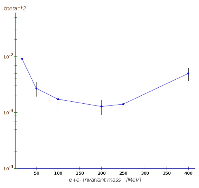
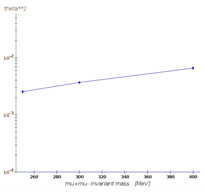
Figure 47: Sensitivity to $\theta{}^{2}$ in the Tulin approachTulin (2014) for the bump-hunt analysis of the processes $\eta\rightarrow\pi^{0}h\;and\;h\rightarrow e^{+}e^{-}$ (left) and $\eta\rightarrow\pi^{0}h\;and\;h\rightarrow\mu^{+}\mu^{-}$ (right) as a function of the mass of a short-lived scalar $h$.

and in Fig. 48 for the two detached-vertex analyses.

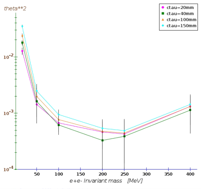
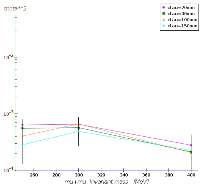
Figure 48: Sensitivity to $\theta{}^{2}$ for the bump-hunt analysis of the processes $\eta\rightarrow\pi^{0}h\;and\;h\rightarrow e^{+}e^{-}$ (left) and $\eta\rightarrow\pi^{0}h\;and\;h\rightarrow\mu^{+}\mu^{-}$ (right) as a function of the mass and $c\tau$ of the a long-lived scalar $h$.

Pospelov parametrization

In this case, see Ref Pospelov , the master formula for $Br(\vartheta^{2})$ (cf. Eq. 105) is given by:

$$BR_{\eta\rightarrow\pi^{0}h}=\frac{\theta^{2}p_{h}\,g_{\eta\pi^{0}h}^{2}}{8\pi m_{\eta}^{2}\Gamma_{\eta}}$$ (114)

where $\Gamma_{\eta}$ is the total width, and $p_{h}$ is the momentum of h particle in the $\eta$ rest frame. The squared amplitude of the process is represented by the parameter $g_{\eta\pi^{0}H}^{2}$:

$$g_{\eta\pi^{0}h}^{2}=\sqrt{\nicefrac{{1}}{{3}}}\times\frac{m_{\pi}^{2}}{\upsilon}\times\frac{m_{d}-m_{u}}{m_{d}+m_{u}}$$ (115)

where: $\upsilon=246\,GeV$. Inserting in Eq. (114) the values of the branching ratio sensitivity derived for each value of the $h$ mass, we obtain the plots for the corresponding sensitivity to the parameter $\theta^{2}$. They are shown in Fig. 49 for the two bump-hunt analyses

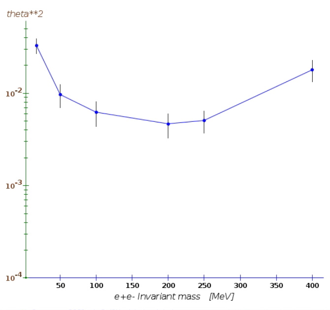
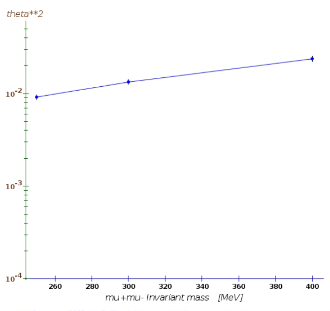
Figure 49: Sensitivity to $\theta{}^{2}$ in the Pospelov approach Pospelov for the bump-hunt analysis of the processes $\eta\rightarrow\pi^{0}h\;\;h\rightarrow e^{+}e^{-}$ (left) and $\eta\rightarrow\pi^{0}h\;\;h\rightarrow\mu^{+}\mu^{-}$ (right) as a function of the mass of a short-lived scalar $h$.

and in Fig. 50 for the two detached-vertex analyses.

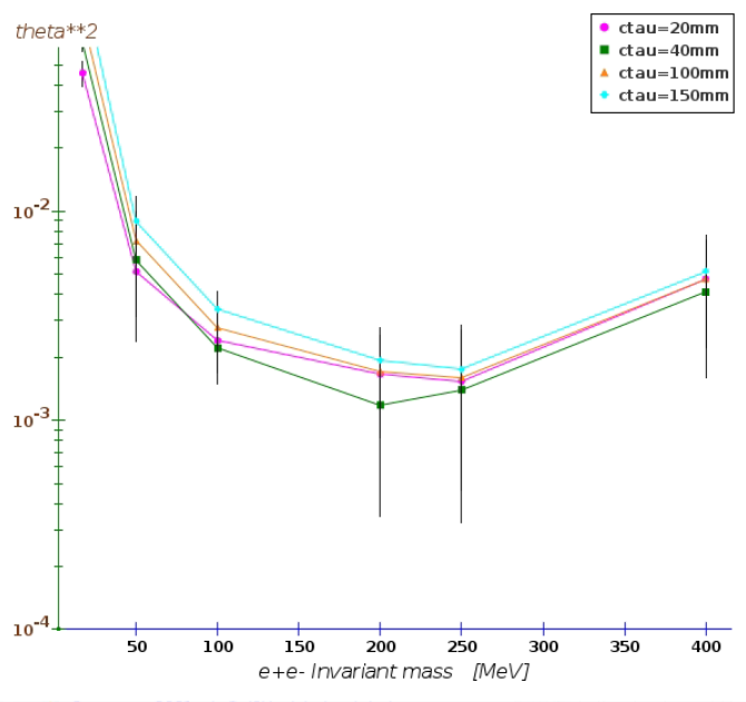
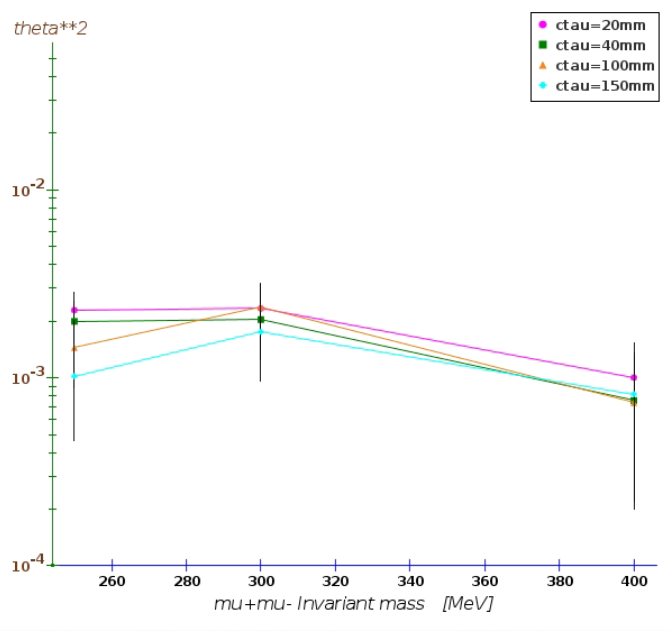
Figure 50: Sensitivity to $\theta{}^{2}$ for the bump-hunt analysis of the processes $\eta\rightarrow\pi^{0}h\;\;h\rightarrow e^{+}e^{-}$ (left) and $\eta\rightarrow\pi^{0}h\;\;h\rightarrow\mu^{+}\mu^{-}$ (right) as a function of the mass and $c\tau$ of the a long-lived scalar $h$.

XI Sensitivity to the Pseudoscalar portal

The Pseudoscalar portal is a very rich sector of BSM physics and several novel theoretical models are predicting the existence of a new pseudoscalar state. Among others, the long-sought Peccei and Quinn (1977c), but never confirmed, Peccei-Quinn model introduces an axion particle which could explain several anomalies recently observed by experiments. Another important class of models falling into this sector is are those which have Axion-Like Particles (ALP’s). These models have extensions of the axion particle with relaxed constraints. The Pseudoscalar portal can be probed at REDTOP via decays of the $\eta$-meson associated to two charged or neutral pions. In this work, we have considered leptonic, radiative, and hadronic decays of the pseudoscalar boson a.

XI.1 Leptonic decays: $a\rightarrow e^{+}e^{-}$ and $a\rightarrow\mu^{+}\mu^{-}$ final states

The processes under study with a leptonic decay mode of the pseudoscalar boson a are:

• $p+Li\rightarrow\eta+X\;with\;\eta\rightarrow\pi^{+}\pi^{-}a\;and\;a\rightarrow e^{+}e^{-}$

• $p+Li\rightarrow\eta+X\;with\;\eta\rightarrow\pi^{0}\pi^{0}a\;and\;a\rightarrow e^{+}e^{-}$

Two different analysis were performed, aiming at testing the performance of different components of the detector: a bump-hunt and a detached-vertex analysis.

XI.1.1 $\eta\rightarrow\pi^{+}\pi^{-}a$: bump-hunt analysis

The same considerations already done for the Vector and Scalar portals hold also for the Pseudoscalar portal. The pseudoscalar boson a was generated in a mass range between 17 MeV and 250 MeV. The boson was decayed promptly in GenieHad, by setting the vertex of the di-lepton in the $\eta$ meson production point. We observed, for this final state, a large background contribution for low mass values for the di-lepton pair originating from photon conversion: $\gamma\rightarrow e^{+}e^{-}$, in the detector material. The photon is usually generated from unreconstructed $\pi^{0}(\eta)\rightarrow\gamma\gamma$ decays of the $\pi^{0}$ and $\eta$ mesons. On the other side, the higher mass range is relatively background free. The second largest background originates from the non-resonant process: $\eta\rightarrow\pi^{+}\pi^{-}e^{+}e^{-}$, which is produced abundantly, as the corresponding branching ratio is 2.68$\times 10^{-4}$.

The full chain of generation-simulation-reconstruction-analysis was repeated for each event set. The TOF and PID systems strongly reduce the background already at the trigger level by a factor of order $\mathcal{\sim}10{}^{4})$. Very generic requirements on the quality of reconstructed particles were applied to the signal and background samples. In particular, no cuts were applied to the reconstructed $e^{+}e^{-}$ vertex. Neutral pions, decaying into $\gamma e^{+}e^{-}$ and $\gamma\gamma$, were reconstructed by considering all combinations of photons, electrons and positrons with an invariant mass within 5 MeV from $\pi^{0}$ mass. This requirement is able to reject most of the combinatoric background, where no $\eta$ mesons are present in the final state. Similarly, photons converting into an $e^{+}e^{-}$ pair where reconstructed by requiring that the invariant mass of the $e^{+}e^{-}$ system was lower than 5 MeV. Finally, the events were required to have a topology consistent with a $\eta\rightarrow\pi^{+}\pi^{-}e^{+}e^{-}$ final state, and an invariant mass compatible with the $\eta$ mass.

The total reconstruction efficiency for this process was found to range between $\sim$1.4% and $\sim$3%, strongly dependent on the di-lepton invariant mass. The reconstruction efficiency was of order $\mathcal{O}(10^{-9})-\mathcal{O}(10^{-9})$ for the Urqmd background.

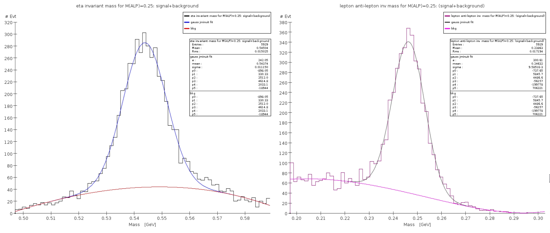
Figure 51: Invariant mass of $\pi^{+}\pi^{-}e^{+}e^{-}$(left) and of the $e^{+}e^{-}$ system (right) for a pseudoscalar boson a with mass M(a)=250 MeV. The plot includes the Urqmd generated background. See text for an explanation of the fitting procedure.

For illustrative purposes, Fig. 51 shows the distribution of the invariant mass of the reconstructed $\pi^{+}\pi^{-}e^{+}e^{-}$ system, for the event set with M(a)=250 MeV merged with the Urqmd generated background. We assumed that BR($\eta\rightarrow\pi^{+}\pi^{-}a$)= $1.4\times 10^{-4}$, while the $\eta$ sample consists of $5\times 10^{8}$ events (corresponding to $4.5\times 10^{-6}$ of the full integrated luminosity). The number of reconstructed signal and background events was obtained form a fit to the $\eta$ meson invariant mass using the sum of a gaussian and a 5th-order polynomial. The integral of the fit function was used to extract the branching ratio sensitivity for this process, according to Eqs. 102-104.

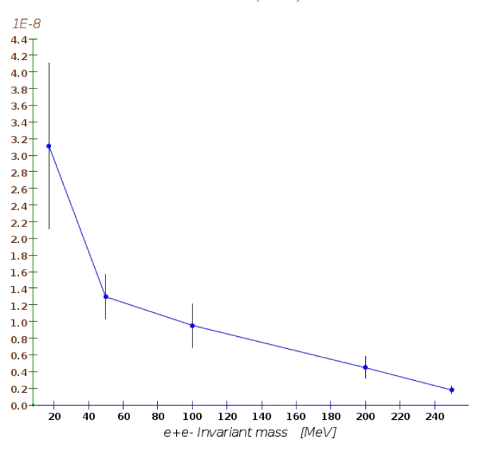
Figure 52: Branching ratio sensitivity for the process $\eta\rightarrow\pi^{+}\pi^{-}a\;with\;a\rightarrow e^{+}e^{-}$ as a function of the pseudoscalar boson mass M(a).

The resulting sensitivity is shown in Fig. 52, as a function of M(a). As expected, the process has a lower sensitivity for values of M(a) below 50 MeV, due to the large contribution of the $\gamma\rightarrow e^{+}e^{-}$ background. On the other side, the sensitivity is of order $\mathcal{O}(10^{-9})$ for higher mass values.

XI.1.2 $\eta\rightarrow\pi^{0}\pi^{0}a$: bump-hunt analysis

This final state requires the reconstruction four particles, two of which (the neutral pions) decay further into at least two more particles. We expect, therefore, a considerably lower detection efficiency when compared to most of the other processes considered here, even just from purely geometrical considerations. For the analysis of this final state, the pseudoscalar $a$ was generated in a mass range between 17 MeV and 250 MeV. The full chain of generation-simulation-reconstruction-analysis was repeated for each set of generated events. Very generic requirements on the quality of reconstructed particles were applied to the signal and background samples.

We observed that the single largest background contribution to this process originates from the decay $\eta\rightarrow\pi^{0}\pi^{0}\pi^{0}$, accounting for more than 50% of the total background surviving the analysis cuts. That process contaminates the signal from either a mis-reconstucted $\pi^{0}\rightarrow\gamma e^{+}e^{-}$ decay or from a $\pi^{0}\rightarrow\gamma\gamma$ decay followed by a $\gamma\rightarrow e^{+}e^{-}$ pair production. However, that source of background has a relatively unambiguous signature and it can be reduced considerably with appropriate kinematic cuts. Consequently, this is one of the channels with the largest branching ratio sensitivity, among those considered in this work, especially for the higher values of M(a), where the surviving background is relatively tame.

No cuts were applied to the reconstructed $e^{+}e^{-}$ vertex. Neutral pions, decaying into $\gamma e^{+}e^{-}$ and $\gamma\gamma$, where reconstructed by considering all combinations of photons, electrons and positrons with an invariant mass within 5 MeV from $\pi^{0}$ mass. This requirement reduces considerably the combinatoric background, where no $\eta$ mesons are present in the final state. Similarly, photons converting into an $e^{+}e^{-}$ pair were reconstructed by requiring that the invariant mass of the $e^{+}e^{-}$ system was lower than 5 MeV. Finally, the events were required to have a topology consistent with a $\eta\rightarrow\pi^{0}\pi^{0}e^{+}e^{-}$ final state, and an invariant mass compatible with the $\eta$ mass.

The total reconstruction efficiency for this process was found to range between $\sim$0.4% and $\sim$2.8%, strongly dependent on the di-lepton invariant mass. The reconstruction efficiency was of order $\mathcal{O}(10^{-13})-\mathcal{O}(10^{-10})$ for the Urqmd background. The number of reconstructed signal and background events was obtained from a fit to the $\eta$ meson invariant mass using the sum of a Gaussian and a 5th-order polynomial.

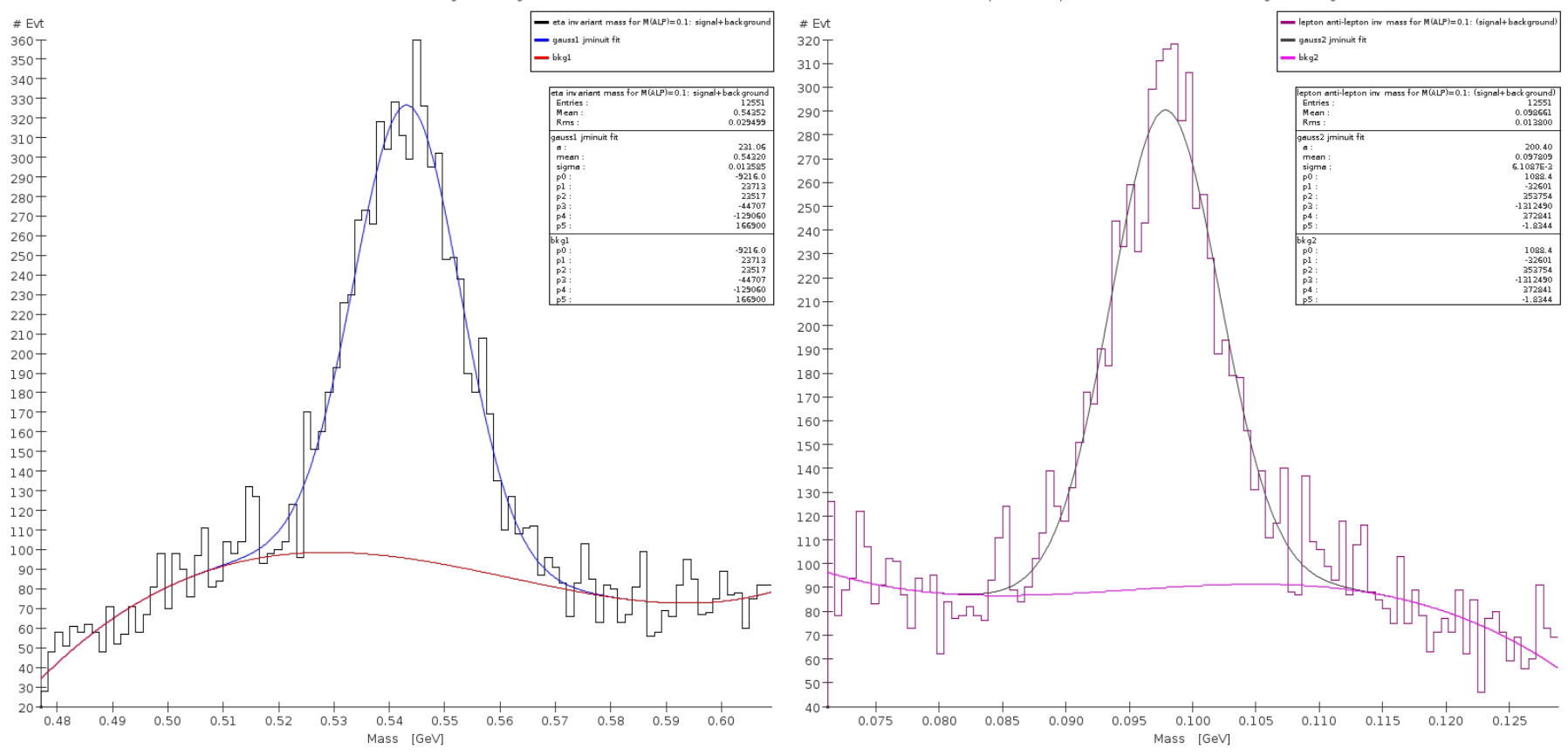
Figure 53: Invariant mass of $\pi^{0}\pi^{0}e^{+}e^{-}$(left) and of the $e^{+}e^{-}$ system (right) for an a with mass M(a)=100 MeV. The plot includes the Urqmd generated background. See text for an explanation of the fitting procedure.

For illustrative purposes, Fig. 53 shows the fit to the invariant mass of the reconstructed $\pi^{0}\pi^{0}e^{+}e^{-}$ for an a mass M(a)=100 MeV, superimposed to the Urqmd generated background. The plots assume a branching ratio BR($\eta\rightarrow\pi^{0}\pi^{0}a$) = $1.4\times 10^{-4}$ and an $\eta$ sample of $5\times 10^{8}$ (corresponding to $4.5\times 10^{-6}$ of the full integrated luminosity).

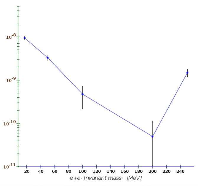
Figure 54: Branching ratio sensitivity for the process $\eta\rightarrow\pi^{0}\pi^{0}a\;with\;a\rightarrow e^{+}e^{-}$ as a function of the pseudoscalar boson a mass.

The resulting sensitivity is shown in Fig. 54, as a function of M(a). As expected, the curve has a lower sensitivity for values of M(a) below 50 MeV, due to the large contamination of the $\gamma\rightarrow e^{+}e^{-}$ background. The sensitivity extends in the $10^{-11}-10^{-9}$ range for higher M(a) values. For values of M(a) near to the kinematic limits, the reconstruction efficiency, and then the sensitivity, degrades again, as the recoiling $\pi^{0}\pi^{0}$ pair has a low momentum and the photons from their decays have a lower probability to be detected or reconstructed.

XI.1.3 $\eta\rightarrow\pi^{0}\pi^{0}a$: detached-vertex analysis

As stressed in the sections above, we expect that a pseudoscalar boson traveling a measurable distance inside the detector will be disentangled more easily from the underlying background, resulting in an improved sensitivity to that process. For the analysis of this channel, the pseudoscalar $a$ was generated with a mass ranging between 17 MeV and 250 MeV. For each value of the mass, the $c\tau$ of the pseudoscalar was varied from 20 mm to 150 mm. A total of 20 event sets were generated and fully reconstructed. The analysis for the kinematic variables follows the same guidelines as for the $bump-hunt$ analysis. Further cuts on the $\chi^{2}$ of a fit to the secondary vertex and on the distance between the primary and secondary vertexes were applied. Since the $\beta\gamma$ boost of the particle depends on the mass of the pseudoscalar particle $a$, those cuts were individually optimized for each event set.

The total reconstruction efficiency for this process, with the additional vertex cuts, was found to range between $\sim$0.2% and $\sim$1.4% for the signal, and of order $\mathcal{O}(10^{-13})-\mathcal{O}(10^{-11})$ for the Urqmd background. The resulting branching ratio sensitivity is shown in Fig. 55, as a function of the invariant mass of the pseudoscalar. The effect of the cuts rejecting the $\pi^{0}\rightarrow\gamma\gamma$ background is clearly visible for low values of M(a), where the sensitivity is degraded below 50 MeV. Furthermore, the $\beta\gamma$ boost for the case M(a)=17 MeV is such that the secondary vertex is often located in the outermost region of the detector, where the charged track reconstruction efficiency is lower. The region of higher mass values is relatively free from combinatorics and Standard Model induced background, and the $\frac{S}{\sqrt{B}}$ ratio is enhanced. The resulting branching ratio sensitivity, for that mass region, extends below $10^{-10}$.

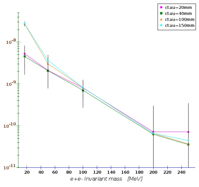
Figure 55: Branching ratio sensitivity for the process $\eta\rightarrow\pi^{0}\pi^{0}a\;with\;a\rightarrow e^{+}e^{-}$ as a function of the mass M(a) and $c\tau$ of the a long-lived pseudoscalar $a$.

XI.2 Radiative decay: $a\rightarrow\gamma\gamma$ final states

As already noted above, in some theoretical models the coupling of the pseudoscalar to leptons is suppressed. In that case, the preferred decay mode of a is into two photons. Therefore, in this work, we have also included the study to the radiative decay mode of the a boson. The process considered is:

• $p+Li\rightarrow\eta+X\;with\;\eta\rightarrow\pi^{+}\pi^{-}a\;and\;a\rightarrow\gamma\gamma$

From the experimental point of view, this final state is affected by a background complementary to the leptonic decay mode. In this case, in fact, the feed-trough from the process $\gamma\rightarrow e^{+}e^{-}$ is almost non-existent, and the low region ofM(a) is expected to exhibit a higher sensitivity than for charged decay modes. On the other side, the $\eta\rightarrow\pi^{+}\pi^{-}\pi^{0}$ process contributes largely, and in an irreducible way, to the background in the mass region around the $\pi^{0}$ mass. In the remaining mass region, most of the background is due to combinatorics associated to QCD processes, and to $\eta\rightarrow\pi^{+}\pi^{-}\pi^{0}$ events, when one of the pions is mis-reconstructed. The second largest background is due to the non-resonant process $\eta\rightarrow\pi^{+}\pi^{-}\gamma$, which survives the event selection when a second photon is found in the event faking the $\eta\rightarrow\pi^{+}\pi^{-}\pi^{0}$ kinematics.

The study of the $a\rightarrow\gamma\gamma$ decay is restricted, in the present work, to the $bump-hunt$ analysis only, since the reconstruction of a detached $\gamma\gamma$ vertex is beyond the current capabilities of the reconstruction software. Later studies will consider also a $detached-vertex$ analysis, since the high-granularity of the ADRIANO2 detector could allow to reconstruct the direction and the impinging point of a photon. The pseudoscalar boson a was generated in a mass range between 17 MeV and 250 MeV. The boson was decayed promptly in GenieHad, by setting the vertex of the two photons to the $\eta$ meson production point. The full chain of generation-simulation-reconstruction-analysis was repeated for each set of generated events. Very generic requirements on the quality of reconstructed particles were applied to signal and background samples.

Neutral pions, decaying into $\gamma e^{+}e^{-}$ and $\gamma\gamma$, where reconstructed by considering all combinations of photons, electrons and positrons with an invariant mass within 5 MeV from $\pi^{0}$ mass. This requirement is able to reject most of the combinatoric background, where no $\eta$ mesons are present in the final state. Similarly, photons converting into a $e^{+}e^{-}$ pair where reconstructed by requiring that the invariant mass of the $e^{+}e^{-}$ system was lower than 5 MeV. The events were, finally, required to have a topology consistent with a $\eta\rightarrow\pi^{+}\pi^{-}\gamma\gamma$ final state, and an invariant mass compatible with the $\eta$ mass.

The final reconstruction efficiency for this process was found to range between $\sim$6% and $\sim$14%, strongly dependent on the $\gamma\,\gamma$ invariant mass. The reconstruction efficiency was of order $\mathcal{O}(10^{-10})-\mathcal{O}(10^{-8})$ for the Urqmd background.

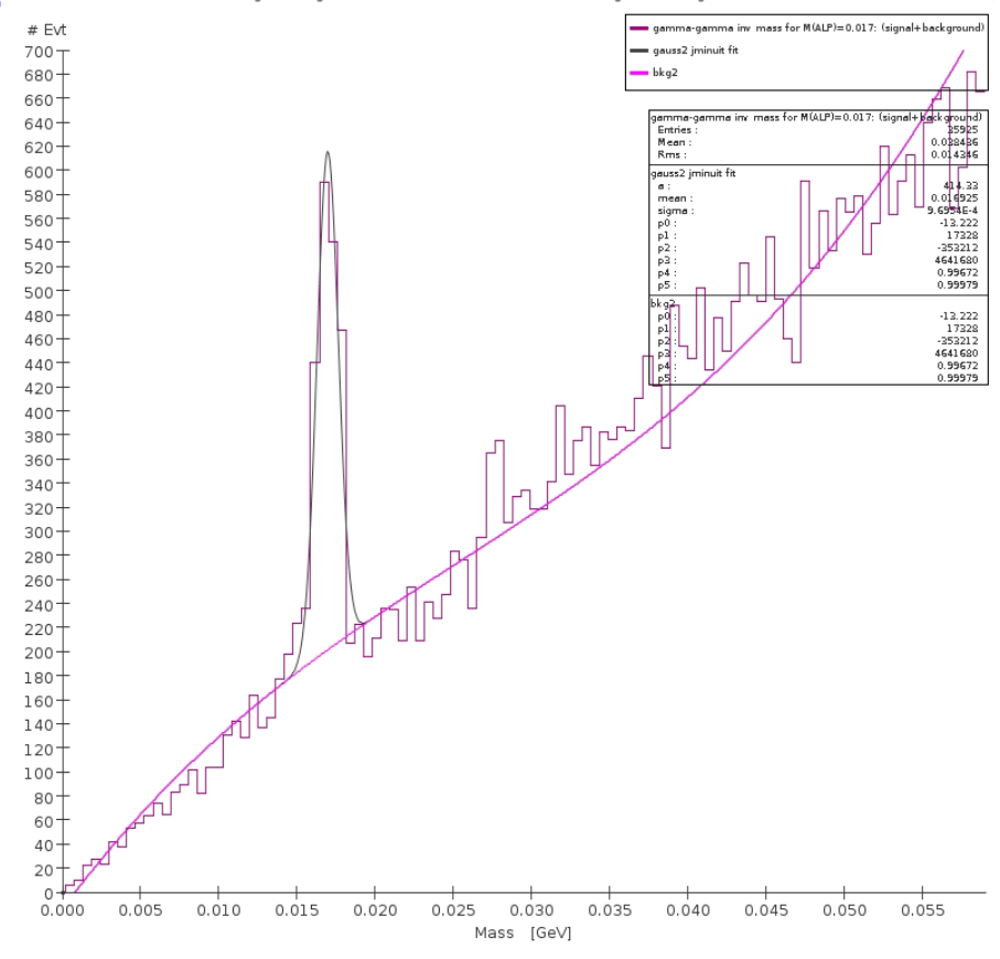
Figure 56: Invariant mass of the $\gamma\,\gamma$ system (right) for a pseudoscalar boson a with mass M(a)=17 MeV. The plot includes the Urqmd generated background. See text for an explanation of the fitting procedure.

For illustrative purposes, Fig. 56 shows the fit to the invariant mass of the reconstructed $\gamma\gamma$ system for a mass of the pseudoscalar M(a)=17 MeV, merged with the Urqmd generated background. The plot assumes a branching ratio BR($\eta\rightarrow\pi^{+}\pi^{-}a$)=$1.4\times 10^{-4}$ and an $\eta$ sample consisting of $5\times 10^{8}$ events (corresponding to $4.5\times 10^{-6}$ of the full integrated luminosity). The number of reconstructed signal and background events was obtained form a fit to the $\eta$ meson invariant mass using the sum of a Gaussian and of a 5th-order polynomial. The integral of the fitted function is used to extract the branching ratio for this process.

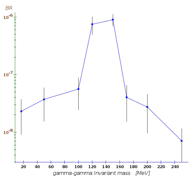
Figure 57: Branching ratio sensitivity for the process $\eta\rightarrow\pi^{+}\pi^{-}a\;with\;a\rightarrow\gamma\gamma$ as a function of the mass of the pseudoscalar boson a

.

The sensitivity obtained from this analysis is shown in Fig. 57, as a function of the pseudoscalar boson a mass. As expected, the region around the $\pi^{0}$ mass has a much lower sensitivity, due to the large and irreducible background deriving from the non-resonant $\eta\rightarrow\pi^{+}\pi^{-}\pi^{0}$ process.

XI.3 Sensitivity to selected theoretical models

QCD axions have been suggested as a natural solution to the strong CP problem Weinberg (1978b). Current QCD axion models are restricted to the sub-eV range masses for the axion (although special variants of the QCD axion are also viable in the MeV mass range; see Alves and Weiner (2018)). A generalization of the minimal model to axion-like particles (ALPs) Jaeckel and Ringwald (2010) allows for models with more massive particles. ALPs can be explored in REDTOP via $\eta/\eta^{\prime}\rightarrow\pi^{0}\pi^{0}a$ and $\eta/\eta^{\prime}\rightarrow\pi^{+}\pi^{-}a$ processes. Depending on the model and the mass of the decaying meson, the ALP can be observed in $a\rightarrow\gamma\gamma$, $a\rightarrow\pi\pi\pi$, $a\rightarrow l^{+}l^{-}.$

Three models, related to the pseudoscalar portal, are currently under consideration by REDTOP: the piophobic axion model, the axion-like particles with quark dominance, and axion-like particles with gluon dominance. It should be noted that all of these models require UV completion at an appropriate scale.

XI.3.1 Sensitivity to Axion-Like Particles

For the discussion of this class of models, we follow the formalism presented in Sec. III.1.5. The relevant parameters in this model are the coupling constants $c_{GG}$, $c_{q}$ and the ALP decay constant $f_{a}$ defined in Eq. 34. The branching ratio sensitivities have been derived above for the processes $\eta\rightarrow\pi^{0}\pi^{0}a$ and $\eta\rightarrow\pi^{+}\pi^{-}a$, for several decay modes and different values of the decay length of the ALP a. For the determination of REDTOP sensitivity to $c_{GG}$ and $c_{q}$, we made the conservative assumption that the a decays only into Standard Model particles. In that case, the values of the coupling constants are also related to the width of a, and, consequently, to the capability of the detector to reconstruct detached vertices.

Using the branching ratios values shown in Fig. 52 though 57, the corresponding sensitivity curves for $c_{GG}/f_{a}$ and $c_{q}/f_{a}(=c_{QQ}/f_{a})$ are shown in Fig, 58, for the final states considered in this work.

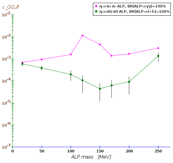
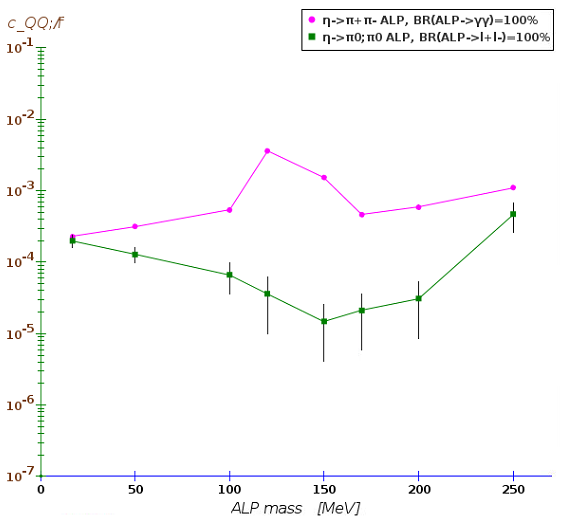
Figure 58: Sensitivity to $c_{GG}/f_{a}$ (left) and $c_{QQ}/f_{a}(=c_{q}/f_{a})$ (right) for the processes $\eta\rightarrow\pi^{+}\pi^{-}a$ and $\eta\rightarrow\pi^{o}\pi^{o}a$ as a function of the mass of a the ALP a. The magenta curves refer to the decay $a\rightarrow e^{+}e^{-}$ while the green curves are for the case: $a\rightarrow\gamma\gamma$. See text for details of the analysis.

XI.3.2 Piophobic QCD axion with mass of 17 MeV/$c^{2}$

Sensitivity studies for this process are performed separately and with different selection cuts, since the underlying theoretical model (cf. Sec. III.1.4) predicts precisely the branching ratio and the momentum distribution of the axion. Furthermore, contrary to the models considered above, which are effective interactions, and typically require UV completion at or below the coupling constant scales, the QCD piophobic axion model does not require external UV completion. The final states considered for this study are:

• $p+Li\rightarrow\eta+X\;with\;\eta\rightarrow\pi^{0}\pi^{0}a\;and\;a\rightarrow e^{+}e^{-}$

• $p+Li\rightarrow\eta+X\;with\;\eta\rightarrow\pi^{+}\pi^{-}a\;and\;a\rightarrow e^{+}e^{-}$

Three separate sets with $\sim$350,000 events were generated, each corresponding to a benchmark parameter sets listed in Table I of Ref. Alves (2021). A forth sample, with the parameters corresponding to the Standard Model prediction, was also generated. Each set was generated with a matrix element obtained from Eq. (53) of Ref.Alves (2021) and $M(a)$=17 MeV. The corresponding $\eta$ sample ranges between $1.9\times 10^{8}$ and $4.2\times 10^{8}$ (or, $3.8\times 10^{-6}$- $7.7\times 10^{-6}$ of the full integrated luminosity), as the branching ratio for this process depends on the values of the parameter set.

The full chain of generation-simulation-reconstruction-analysis was repeated for each set of events. Very generic requirements on the quality of reconstructed particles was applied to the signal and background samples. Neutral pions, decaying into $\gamma e^{+}e^{-}$ and $\gamma\gamma$, where reconstructed by considering all combinations of photons, electrons and positrons with an invariant mass within 5 MeV from $\pi^{0}$ mass. This requirement is able to reject most of the combinatoric background, where no $\eta$ mesons are present in the final state. Similarly, photons converting into a $e^{+}e^{-}$ pair where reconstructed by requiring that the invariant mass of the $e^{+}e^{-}$ system was lower than 5 MeV. The events were, finally, required to have a topology consistent with a $\eta\rightarrow\pi^{0}e^{+}e^{-}$ final state, and an invariant mass compatible with the $\eta$ mass.

The reconstruction efficiencies for this process and for the Urqmd generated background are summarized in Table 26 along with the sensitivity obtained by using Eq. (105) for 3.3$\times 10^{18}$ POT.

Process	Benchmark	Trigger	Trigger	Trigger	Reconstruction	Analysis	Total	BR
	set	L0	L1	L2				sensitivity
$\eta$$\rightarrow\pi^{+}\pi^{-}a\;;\;a\rightarrow e^{+}e^{-}$	B1	$55.28\%$	$21.81\%$	$76.41\%$	75.12%	42.94%	$2.97$%	$2.07\times 10^{-8}$
$\eta$$\rightarrow\pi^{+}\pi^{-}a\;;\;a\rightarrow e^{+}e^{-}$	B2	56.15%	22.32%	76.76%	75.12%	42.83%	3.10%	$1.98\times 10^{-8}$
$\eta$$\rightarrow\pi^{+}\pi^{-}a\;;\;a\rightarrow e^{+}e^{-}$	B3	59.67%	23.06%	79.81%	76.14%	44.03%	3.68%	$1.67\times 10^{-8}$
Urqmd		$21.7\%$	$1.7\%$	$22.2\%$	$0.26$%	1.04%	$2.31\times 10^{-6}$%

Table 26: Reconstruction efficiencies for $\eta$$\rightarrow\pi^{+}\pi^{-}a\;;\;a\rightarrow e^{+}e^{-}$ for the piophobic axion model Alves (2021) and for the Urqmd generated background

The $\eta$ content in each group is extracted with a fit using the sum of a Gaussian and a 5th-order polynomial, and by integration of the Gaussian signal after background subtraction. The signal and background content for the events corresponding to the benchmark set #1, is shown in Fig. 60. The statistical error from the fit is used to derive the uncertainty of the branching ratio. The errors for the three benchmark sets are summarized in the third column of Table 27.

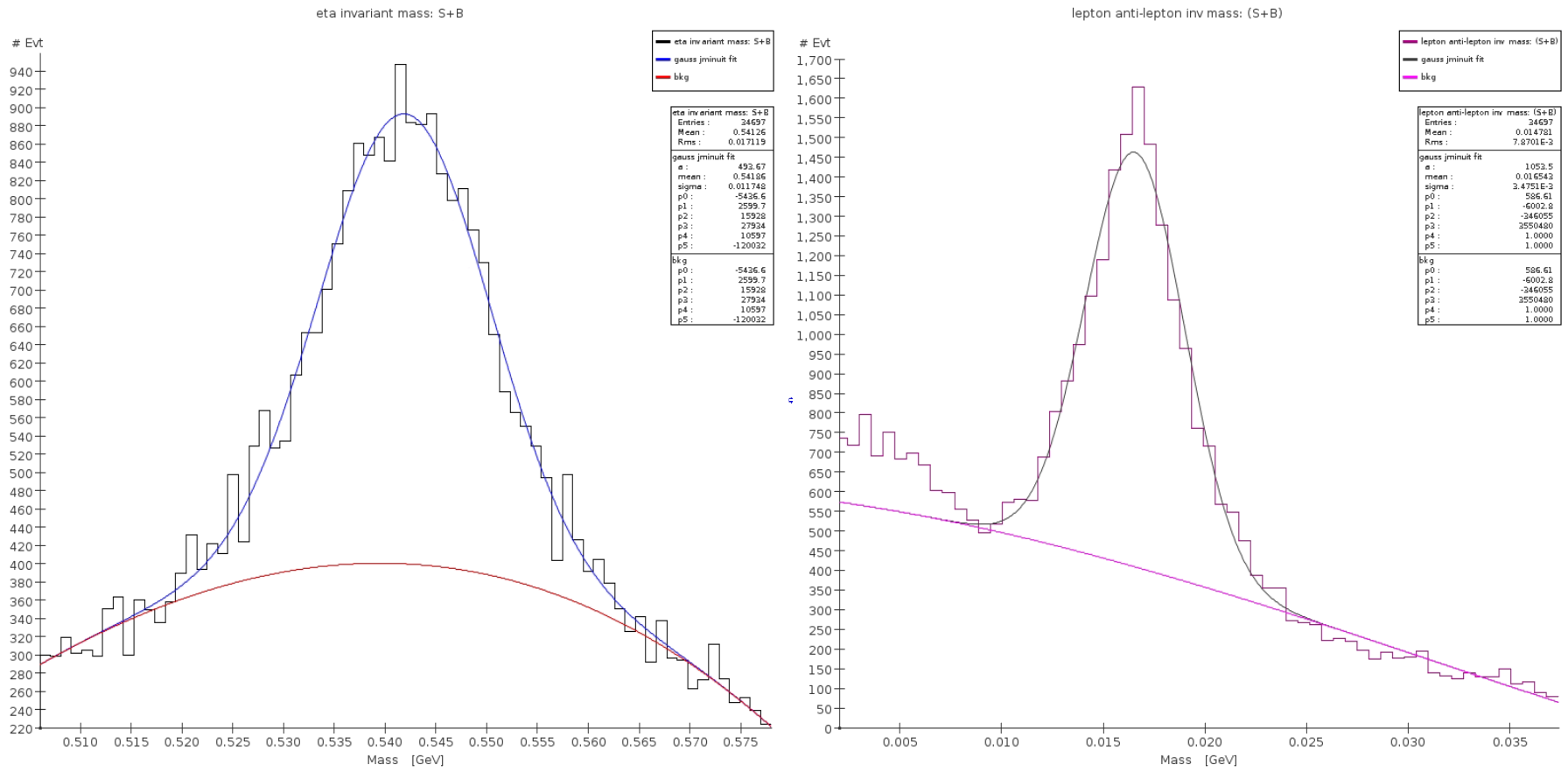
Figure 59: Invariant mass of $\pi^{+}\pi^{-}e^{+}e^{-}$(left) and of the $e^{+}e^{-}$ system (right) for a piophobic axion. The plots includes the Urqmd generated background. See text for an explanation of the fitting procedure.

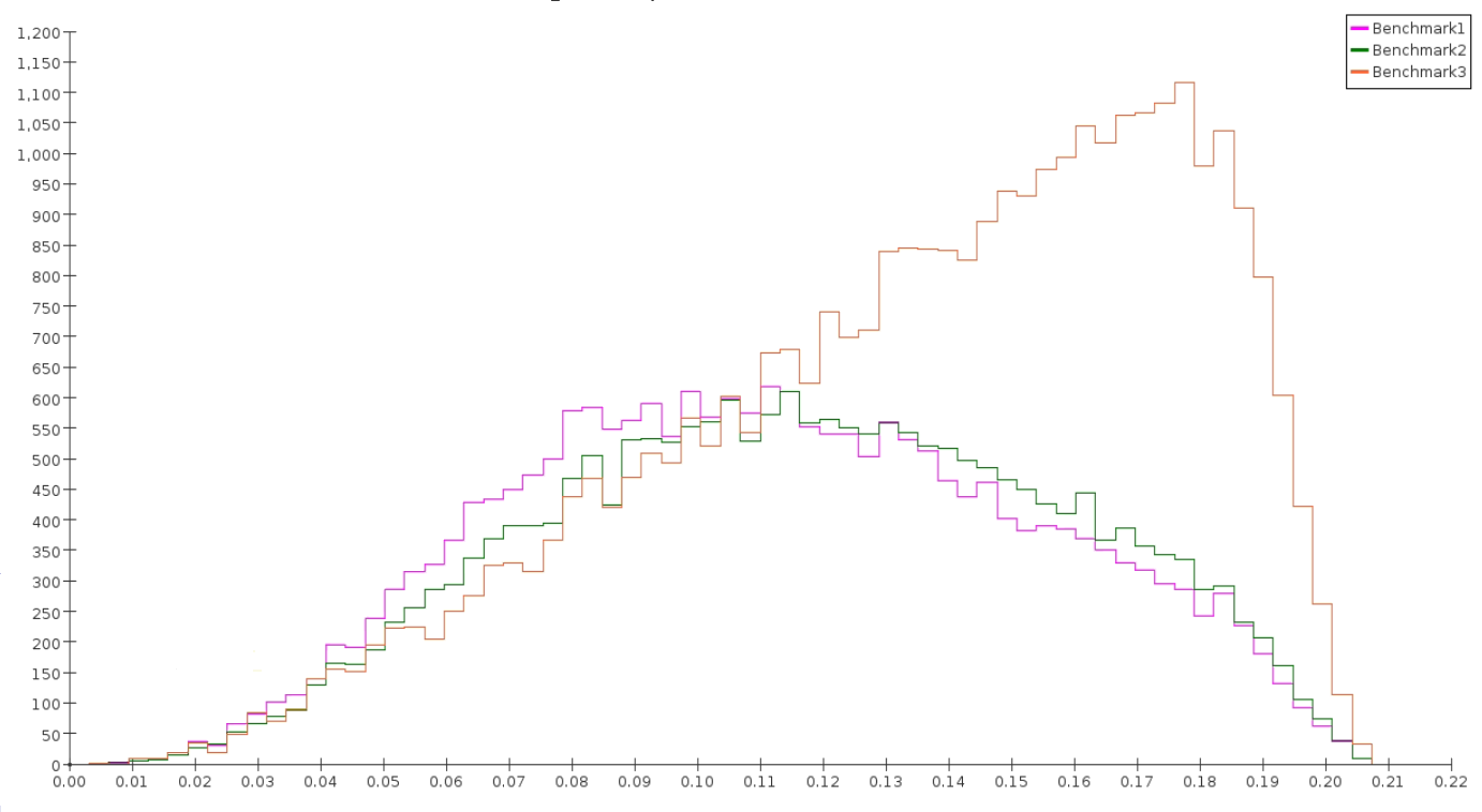
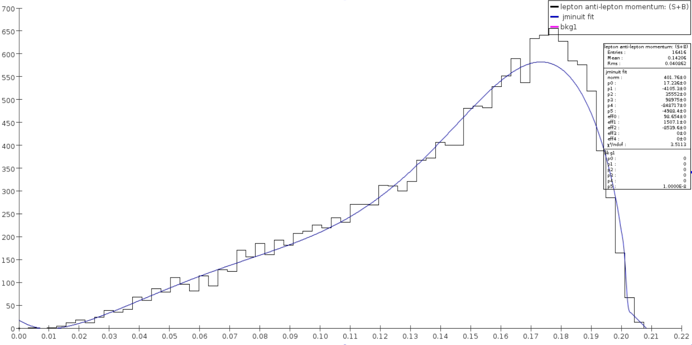
Figure 60: The axion momentum in the $\eta$ CM system for the three parameter sets considered in the study (left). Fit to the distribution corresponding to the benchmark set #3 (right) from Ref. Alves (2021). See text for an explanation of the fitting procedure.

Final cuts of, respectively 16 MeV and 4 MeV were applied around the invariant mass of the $\pi^{+}\pi^{-}e^{+}e^{-}$ systems and of the reconstructed axion. Those cuts aim at increasing the purity of the signal before performing the final fit to extract the model parameters. In order to estimate the sensitivity of the experiment to this model, the distribution of the axion momentum is fitted using the the theoretical matrix element from Ref. Alves (2021), combined with a second degree polynomial describing the background. To take into account the non-uniform acceptance of the detector, a multiplicative polynomial efficiency was used in the fit. The analysis was repeated for each of the three sets of events generated. The fit to the axion momentum distribution corresponding to the benchmark set #3 is shown on the right side of Fig. 60. The resulting $\chi^{2}$ probability for the three sets is summarized in Table 27.

POT	$\eta$$\rightarrow\pi^{+}\pi^{-}a\;;\;a\rightarrow e^{+}e^{-}$	BR	$\chi^{2}$/ndof
	Benchmark set	statistical error
1.1$\times 10{}^{13}$	B1	1.5%	3.2
1.3$\times 10{}^{13}$	B2	1.4%	2.9
5.6$\times 10{}^{12}$	B3	2.1%	3.5

Table 27: Goodness of fit of the P_axion distribution using the matrix element from Ref. Alves (2021)

It is worth noting that an interesting possibility of a QCD axion with small $f_{a}$ opens additional avenues for $a$ searches. In particular, the property of piophobia, together with a 17 MeV mass imply a rather large decay rate of a neutral pion to three axions, $\pi^{0}\to 3a$. This decay has a branching ratio of $10^{-3}$ Hostert and Pospelov (2022), and will create three electron-positron pairs as each $a$ decays. Therefore, one can expect $2\pi 3(e^{+}e^{-})$ decay mode of $\eta$ with the branching of $\sim 10^{-5}-10^{-7}$. Moreover, if $a$’s are discovered in a singles production channel, the exploration of multiple $a$ production can support or refute the hypothesis of the QCD axion, as nonlinear self-interaction terms of $a$ are necessary for a QCD axion and are fixed by the requirements of the Peccei-Quinn invariance.

XII Sensitivity to the Heavy Neutral Lepton portal

XII.1 $\eta\rightarrow\pi^{0}H\;;\;H\rightarrow\nu N_{2}\;;\;N_{2}\rightarrow N_{1}h^{\prime}\;;\;h^{\prime}\rightarrow e^{+}e^{-}$: Detached vertex analysis

The studies presented in this Section are based on the model discussed in Sec. III.1.2. The benchmark parameters of that model are such that the process is kinematically allowed only for $\eta^{\prime}$ mesons. To test the branching ratio sensitivity at REDTOP, the values listed in Table 28 are used instead:

$m_{N_{1}}$	$m_{N_{2}}$	$m_{N_{3}}$	$y_{e(\mu)}^{h^{\prime}}\!\!\times\!\!10^{4}$	$y_{e(\mu)}^{H}\!\!\times\!\!10^{4}$
85 MeV	$130$ MeV	$10$ GeV	$0.23(1.6)$	$2.29(15.9)$
$m_{h^{\prime}}$	$m_{H}$	$\sin\delta$	$y_{\nu_{\!i2}}^{h^{\prime}(H)}\!\!\times\!\!10^{3}$	$\lambda_{N_{\!12}}^{h^{\prime}(H)}\!\!\times\!\!10^{3}$
17 MeV	250 MeV	$0.1$	$1.25(12.4)$	$74.6(-7.5)$

Table 28: Benchmark parameters for REDTOP.

The branching ratios of the decay modes of $H$ are recomputed according to the new parameters. The new values are as follow:

$$\!\!\!\!\!\!\!\!\!\!\!\!\!\!\!\!\!\!\!\!\!\!{\rm BR}(H\rightarrow\nu_{i}N_{2})=96.93\%,\leavevmode\nobreak\ {\rm BR}(H\rightarrow N_{1}N_{2})=2.90\%,\leavevmode\nobreak\ {\rm BR}(H\rightarrow\mu^{+}\mu^{-})=0.15\%,$$ (116)

$$\!\!\!\!\!\!\!\!\!\!\!\!\!\!\!\!\!\!\!\!\!\!{\rm BR}(H\rightarrow e^{+}e^{-})=0.021\%,\leavevmode\nobreak\ \leavevmode\nobreak\ \!{\rm BR}(H\rightarrow\gamma\gamma)=5.36\times 10^{-6}\%.$$ (117)

For the parameters in Table 28, the total decay width of $H$, $h^{\prime}$, and $N_{2}$ are $2.52\times 10^{-6}$ GeV, $3.56\times 10^{-13}$ GeV, and $2.07\times 10^{-5}$ GeV, respectively. Hence all the particles will decay inside the REDTOP. However, the width of $h^{\prime}$ corresponds to $c\tau=620\leavevmode\nobreak\ \mu m$ so that the $e^{+}e^{-}$ pair has a detached secondary vertex, eventually resolvable with an appropriate choice of a vertex detector.

The event generation for this process is based on the model described in Sec. III.2.1 for a reduced $\eta$ sample corresponding to $\sim$2.7$\times$$10^{13}$ POT (namely, to $\sim$2.7$\times$$10^{-5}$ of the integrated luminosity foreseen for the experiment). The full chain of generation-simulation-reconstruction-analysis was repeated for each set of the parameters and for the parameters corresponding to the Standard Model prediction. The largest background contaminating the signal is due to the decays $\gamma\rightarrow e^{+}e^{-}$ and $\pi^{0}\rightarrow\gamma e^{+}e^{-}$, paired to an extra photon, usually generated from the decay of a $\pi^{0}$ or an $\eta$ meson, which mimic a $\pi^{0}$. Very generic requirements on the quality of reconstructed particles was applied to the signal and background samples. Neutral pions, decaying into $\gamma e^{+}e^{-}$ and $\gamma\gamma$, where reconstructed by considering all combinations of photons, electrons and positrons with an invariant mass within 5 MeV from $\pi^{0}$ mass. This requirement is able to reject most of the combinatoric background with no $\eta$ mesons in the final state. Similarly, photons converting into a $e^{+}e^{-}$ pair where reconstructed by requiring that the invariant mass of the $e^{+}e^{-}$ system was lower than 5 MeV. From the experimental point of view, this final state suffer from the presence of three missing particles. Therefore, no constraint could be imposed on the invariant mass of the detected particles. On the other side, the presence of a fully reconstructed $e^{+}e^{-}$ pair with a detached vertex could help to reject the Standard model background. Therefore, on the $\chi^{2}$ from the fit of two charged tracks to a common vertex and on the distance between the primary and secondary vertexes were applied. The goal of those cuts was to remove events with particles originating from the $\eta$ production point. The reconstruction efficiencies for this process and for the Urqmd generated background are summarized in Table 29.

Process	Trigger	Trigger	Trigger	Reco	Analysis	Total	BR
	L0	L1	L2				Sensitivity
$\eta\rightarrow\pi^{0}H\;;\;H\rightarrow\nu N_{2}\;;$ $\;N_{2}\rightarrow N_{1}h^{\prime}\;;\;h^{\prime}\rightarrow e^{+}e^{-}$	$38.5\%$	$22.6\%$	$80.5\%$	$91.1$%	$19.6\%$	$1.3$%	$2.7\times 10^{-7}\pm 7\times 10^{-9}$
Urqmd	$21.7\%$	$1.7\%$	$22.2\%$	$47.7$%	$0.17\%$	$6.6\times 10^{-5}$%

Table 29: Reconstruction efficiencies and branching ratio sensitivity for $\eta\rightarrow\pi^{0}H\;;\;H\rightarrow\nu N_{2}\;;\;N_{2}\rightarrow N_{1}h^{\prime}\;;\;h^{\prime}\rightarrow e^{+}e^{-}$ and for the Urqmd generated background with the parameters used in Table 29.

XII.2 Sensitivity to selected theoretical models

For the studies presented in this work, we have considered only one theoretical model, which is discussed below.

XII.2.1 Two-Higgs doublet model

The parameters $\lambda_{u}$ and $\lambda_{d}$ for this model, along with the branching ratios predicted for decay channels $\eta^{(\prime)}\to\pi^{0}S$ are discussed in Sec. III.1.2. For the Two-Higgs doublet model considered in this work Abdallah et al. (2021), the branching ratio, in the assumption that $\lambda_{u}=\lambda_{d}$, is predicted to be of order $\mathcal{O}(10^{-13})$, which is below REDTOP sensitivity in the present run. The situation is different when $\lambda_{u}\neq\lambda_{d}$. In that case, assuming the values for the branching ratios of the $H$ defined in Eqs. (116),(117), and the branching ratios of the $N_{2}$ and $h^{\prime}$ defined in Eqs. (31),(32) we derive the sensitivity to $(\lambda_{u}-\lambda_{d})^{2}$ case from the branching ratio sensitivity derived in Sec. XII and from Eq. (111). The final value is summarized in Table 30

Process	$m_{h^{\prime}}$	$m_{N_{2}}$	Analysis	$(\lambda_{u}-\lambda_{d})^{2}$
	[MeV]	[MeV]		sensitivity
$\eta\rightarrow\pi^{0}H\;;\;H\rightarrow\nu N_{2}\;;\;N_{2}\rightarrow N_{1}h^{\prime}\;;\;h^{\prime}\rightarrow e^{+}e^{-}$	17	250	detached vertex	$3.89\times 10^{-12}$

Table 30: Sensitivity to $(\lambda_{u}-\lambda_{d})^{2}$ for the Two-Higgs doublet model Abdallah et al. (2021).

and shown in Fig. 61 superimposed to the prediction of the theoretical model.

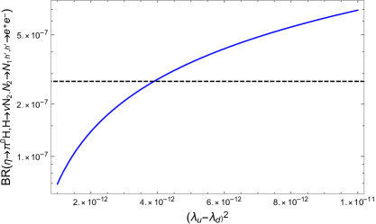
Figure 61: Branching ratio for the process $\eta\rightarrow\pi^{0}H\;;\;H\rightarrow\nu N_{2}\;;\;N_{2}\rightarrow N_{1}h^{\prime}\;;\;h^{\prime}\rightarrow e^{+}e^{-}$ predicted by the Two Higgs Doublet model Abdallah et al. (2021) as a function of $(\lambda_{u}-\lambda_{d})^{2}$. The dashed line corresponds to the experimental limit for REDTOP with an integrated luminosity of 3.3$\times 10^{18}$ POT.

XII.3 Concluding remark

The reconstruction of the process $\eta\rightarrow\pi^{0}H\;;\;H\rightarrow\nu N_{2}\;;\;N_{2}\rightarrow N_{1}h^{\prime}\;;\;h^{\prime}\rightarrow e^{+}e^{-}$ is particularly challenging at REDTOP, because the decay chains contains two missing particles: namely, the two neutral leptons $N_{1}$ and $N_{2}$. Furthermore, the decay length of the $h^{\prime}$ scalar is less than 1 mm, which is resolved poorly by the fiber-tracker detector implemented in the current studies. All that is reflected in a considerably lower sensitivity to this channel, when compared to most of the other processes analyzed in this work, where all the particles in the final state are visible. A better vertex detector, such as the ITS3 option discussed in Sec. VI.4.1) which has the ability to resolve with a higher efficiency the detached vertex of the $h^{\prime}$ scalar, could improve considerably REDTOP sensitivity to this channel.

XIII Tests of Conservation Laws

XIII.1 CP-violation studies from Dalitz plot mirror asymmetry in $\eta\rightarrow\pi^{+}\pi^{-}\pi^{0}$

The event generation for this process is based on the model described in Sec. III.2.1. Several event samples were generated, corresponding to different values of the parameters consisting of $\sim 1.1\times 10^{8}$ $\eta$ mesons from 3.3$\times 10^{12}$ POT (corresponding to 1.0$\times 10^{-6}$ of the total integrated luminosity foreseen for the experiment).

As discussed in detail in Sec. III.2.1), the matrix element generating the asymmetry, in the Gardner-Shi parametrization scheme (cf. Ref.Gardner and Shi (2020)), depends on two complex parameters $\bar{\alpha}$ and $\bar{\beta}$. In order to estimate the sensitivity of REDTOP to this process, we have scanned the real and the imaginary parts of $\bar{\alpha}$ and $\bar{\beta}$ in steps of 1.5 $\sigma$ around the values obtained by authors from a fit to Kloe-II data (eq. 14 in Ref.Gardner and Shi (2020)). An additional event set was generated, with the parameters corresponding to the Standard Model prediction.

The full chain of generation-simulation-reconstruction-analysis was repeated for each event set. Very generic requirements on the quality of reconstructed particles was applied to the signal and background samples. Neutral pions, decaying into $\gamma e^{+}e^{-}$ and $\gamma\gamma$, where reconstructed by considering all combinations of photons, electrons and positrons with an invariant mass within 5 MeV from $\pi^{0}$ mass. Finally, the events were required to have a topology consistent with a $\eta\rightarrow\pi^{+}\pi^{-}\pi^{0}$ final state, and an invariant mass compatible with the $\eta$ mass. A final kinematic cut of, respectively 6 MeV and 5 MeV around the invariant mass of the three pions and of the reconstructed $\pi^{0}$ meson was applied to increase the purity of the signal used for the analysis of the Dalitz plot. The largest background for this channel was found to originate from combinatorics $p+Li\rightarrow\pi^{+}\pi^{-}\pi^{0}+X$, when the invariant mass of the three pions survived the kinematic cuts and it was consistent with the decay of the $\eta$ meson. The reconstruction efficiencies for this process and for the Urqmd generated background are summarized in Table 31

Process	Trigger	Trigger	Trigger	Reconstruction	Analysis	Total
	L0	L1	L2
$\eta$$\rightarrow\pi^{+}\pi^{-}\pi^{0}$	$48.6\%$	$10.9\%$	$82.7\%$	$96.3$%	$6.46$%	$2.7\times 10^{-2}$%
Urqmd	$21.7\%$	$1.7\%$	$22.2\%$	$4.3$%	$0.93$%	$3.2\times 10^{-5}$%

Table 31: Reconstruction efficiencies for $\eta\rightarrow\pi^{+}\pi^{-}\pi^{0}$ and for the Urqmd generated background

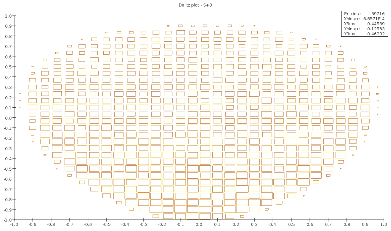
Figure 62: Dalitz plot of $\eta\rightarrow\pi^{+}\pi^{-}\pi^{0}$ combined with the Urqmd background.

A total of 18 Dalitz plots were generated, corresponding to the CP-violating parameters described above. The Dalitz plot of $\eta\rightarrow\pi^{+}\pi^{-}\pi^{0}$ for the set of parameters corresponding to Kloe-II is shown in Fig. 62.

The parameters obtained from the fits to the Standard Model configuration, where the CP-violating parameters are all zero, are summarized in Table 32. The same binning of the Dalitz plot as in KLOE experiment was used with 372 bins in the $(X,Y)$ plane.

#Rec. Events	Re($\alpha$)	Im($\alpha$)	Re($\beta$)	Im($\beta$)	p-value
$10^{8}$ (no-bkg)	$3.3\times 10^{-1}$	$3.7\times 10^{-1}$	$4.4\times 10^{-4}$	$5.6\times 10^{-4}$	$17$%
Full stat. (no-bkg)	$1.9\times 10^{-2}$	$2.1\times 10^{-2}$	$2.5\times 10^{-5}$	$3.2\times 10^{-5}$	$17$%
Full stat. (100%-bkg)	$2.3\times 10^{-2}$	$3.0\times 10^{-2}$	$3.5\times 10^{-5}$	$4.5\times 10^{-5}$	$16$%

Table 32: Sensitivities – statistical uncertainties for the two complex Dalitz plot CPV parameters $\alpha$ and $\beta$ according to Ref. Gardner and Shi (2020). The generated distribution is the Standard Model configuration i.e., $\alpha,\beta=0$. The fit reproduces the generated input, with the p-values given in the last column, within the statistical uncertainties given for the real and imaginary parts of the parameters as given in the columns 2–5.

All parameters are consistent with the generated values, within the fit error. The latter have the same order of magnitude as those obtained from a fit to KLOE data, using a comparable event size (cf. Ref.Gardner and Shi (2020)). The projected sensitivities for the event sample obtained with the full integrated luminosity of $3.3\times 10^{18}$ POT (corresponding to $3\times 10^{10}$ reconstructed $\eta\to\pi^{+}\pi^{-}\pi^{0}$ events) are given for case of no-background and 100%-background contamination. They are much smaller than from the KLOE result and potentially sufficient to detect non-zero values of the CP-violating parameters.

XIII.2 CP-violation studies from the asymmetry of the decay planes of $\eta\rightarrow\pi^{+}\pi^{-}e^{+}e^{-}$

The formal aspects of this process, including the relationship between the CP-violating parameters and the observable, has been discussed in details in Sec III.2.2

This measurement has been previously attempted by the WASA-at-COSY experiment Bargholtz et al. (2007) using an event sample containing 3 × 10⁷ $\eta$ mesons. The sensitivity to this process is determined by examining at the asymmetry:

$$A_{\phi}=\frac{N(\sin\phi\cos\phi>0)-N(\sin\phi\cos\phi<0)}{N(\sin\phi\cos\phi>0)+N(\sin\phi\cos\phi<0)}$$ (118)

where $\phi$ is the angle between the decay planes of the lepton-antilepton pair and the two charged pions (see Fig. 63).

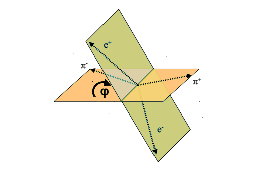
Figure 63: Definition of the dihedral angle $\phi$ for the $\eta\rightarrow\pi^{+}\pi^{-}e^{+}e^{-}$ decay in rest frame of the the $\eta$ meson.

Five event samples, each corresponding to 6$\times 10^{12}$ POT (or $2\times 10^{8}$ $\eta$-mesons), were generated using $GenieHad$ with $<sign(sin(\phi)cos(\phi)>$ in the range [0, $4\times 10^{-2}$]. The full chain of generation-simulation-reconstruction-analysis was repeated for each set of the parameters and for the parameters corresponding to the Standard Model prediction. The largest background contaminating the signal originates from the decays $\gamma\rightarrow e^{+}e^{-}$ and $\pi^{0}\rightarrow\gamma e^{+}e^{-}$, simultaneously with the presence of two extra charged pions generated in the beam-target collision. Very generic requirements on the quality of reconstructed particles were applied to signal and background samples.

Neutral pions, decaying into $\gamma e^{+}e^{-}$ and $\gamma\gamma$, where reconstructed by considering all combinations of photons, electrons and positrons with an invariant mass within 5 MeV from $\pi^{0}$ mass. Successfully reconstructed $\pi^{0}$’s were removed from the event. Similarly, the photons converting in the detector material were reconstructed and removed from the event. Finally, the events were required to have a topology consistent with a $pi^{+}\pi^{-}e^{+}e^{-}$ final state, and an invariant mass compatible with the $\eta$ mass. The above selection rules were able to remove a large fraction of background events.

The reconstruction efficiencies for the signal, averaged over the five event sets, and for the Urqmd generated background are summarized in Table 33 along with the sensitivity to the branching ratio obtained using Eq. (105) for the full integrated beam current of $3.3\times 10^{18}$ POT.

Process	Benchmark	Trigger	Trigger	Trigger	Reco	Analysis	Total	BR
	set	L0	L1	L2				sensitivity
$\eta$$\rightarrow\pi^{+}\pi^{-}e^{+}e^{-}$	average.	$64.0$	$34.2\%$	$83.1\%$	78.9%	55.8%	$8.0$%	$4.9\times 10^{-9}$
Urqmd		$21.7\%$	$1.7\%$	$22.2\%$	$0.26$%	4%	$8.6\times 10^{-6}$%

Table 33: Reconstruction efficiencies for the $\eta\rightarrow\pi^{+}\pi^{-}e^{+}e^{-}$ final state and for the Urqmd generated background. The values are averaged over the five benchmark sets.

The $sin\phi cos\phi$ distribution for the events belonging to the $<sign(sin(\phi)cos(\phi)>=0$ set and surviving the analysis cuts is shown in Fig. 64 along with the invariant mass of the reconstructed $\pi^{+}\pi^{-}e^{+}e^{-}$ systems. The combinatorics background is well fitted under the $\eta$ peak.

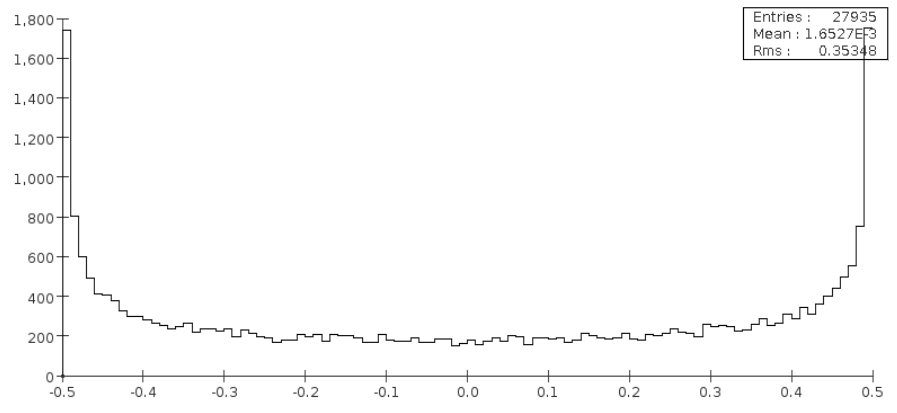
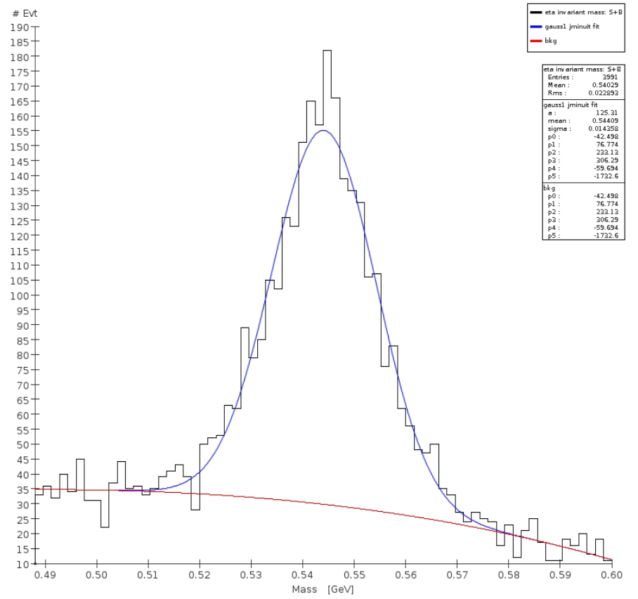
Figure 64: $sin\phi cos\phi$ distribution (left) and invariant mass of the $\pi^{+}\pi^{-}e^{+}e^{-}$ system (right) for the set of events with $<sign(sin(\phi)cos(\phi)>=0$. The histograms include the Urqmd background. See text for an explanation of the fitting procedure.

For the next step of the analysis, the data from each set were divided into separate $sin\phi cos\phi$>0 and $sin\phi cos\phi<0$ groups. The $\eta$ content in each group was extracted with a fit using the sum of a Gaussian and a 5th-order polynomial. The measured asymmetry is plotted in Fig. 65 vs the true value for each of the five event sets. The diluting effect of the background is clearly observed since the measured asymmetry is attenuated by a factor of $\sim 65\%$. We conclude that the measured asymmetry for the samples considered is larger than the statistical error (which is the dominant component in the measurements by WASA and KLOE experiments) for values of the true asymmetry larger than approximately $1\times 10^{-2}$. This estimate is consistent with the results obtained by the WASA with an event sample a factor 100 smaller, as their measurement has a ten-times larger statistical error. When the total integrated luminosity of $3.3\times 10^{18}$ POT foreseen for REDTOP is taken into account, we expect that the statistical error will be reduced by more than two orders of magnitude, corresponding to a contribution to the $A_{\phi}$ sensitivity smaller than $\sim 10^{-4}$. Therefore, we conclude that the uncertainty on the measured asymmetry will be, most likely, dominated by the systematic error.

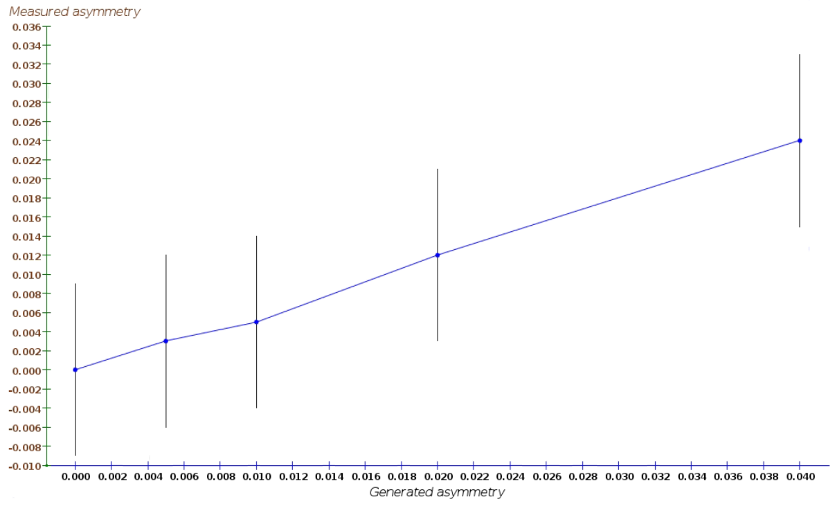
Figure 65: Sensitivity to $sin\phi cos\phi$ asymmetry for $\eta\rightarrow\pi^{+}\pi^{-}e^{+}e^{-}$. The errors in the plot are statistical only.

XIII.3 CP-violation studies in the decays $\eta\rightarrow\mu^{+}\mu^{-}$

A detailed discussion on probing CP-violation in leptonic $\eta$ decays can be found in Sec. III.2.4 and Sec. V.1 along with the formulae relating the Wilson coefficients (carrying the CP-violating parameters) to the observable quantities.

The sensitivity to this process is studied by measuring the polarization of the muon reconstructed from the following process:

• $p+Li\rightarrow\eta+X\;with\;\eta\rightarrow\mu^{+}\mu^{-}$

The two relevant observables are the two asymmetries defined in Eqs.(75,76), that carry the information from the muon polarization. The $\eta\rightarrow\mu^{+}\mu^{-}$ process is considered as the golden mode to explore $CP-violation$ since the operator responsible for the asymmetry has the largest coupling to the observables. In order to measure the angles $\theta$ and $\phi$, a full reconstruction of the $\mu^{\pm}\rightarrow e^{\pm}\nu\overline{\nu}$ decay needs to be performed. This capability will be implemented soon in REDTOP Offline software. For the moment, only a rough estimate of the expected polarization efficiency will be made.

The event generation for this process is based on the model described in Sec. III.2.6. A sample consisting of $\sim 8.6\times 10^{9}$ $\eta$ mesons from 2.6$\times 10^{14}$ POT (corresponding to 7.8$\times 10^{-5}$ of the total integrated luminosity foreseen for the experiment). The full chain of generation-simulation-reconstruction-analysis described in Sec. VII.4 was repeated for each event set. Very generic requirements on the quality of reconstructed particles were applied to the signal and background samples. The main background for this channel is due to the non-resonant decay $\eta\rightarrow\gamma\mu^{+}\mu^{-}$ which occurs with a relatively large branching ratio of $3.1\times 10^{-4}$. The second largest background originates from charged pions, mis-identified as muons. With the present detector configuration, the $\pi$/$\mu$ mis-identification probability was estimate to be $\sim$3.5% (or, $\sim$0.12% for mis-identifying both leptons). Since the probability of generating two charged pions in the target is almost 11% (see, for example, Fig. 17), we expect that about $\sim 3.3\times 10^{11}$ events could possibly fake a $\eta\rightarrow\mu^{+}\mu^{-}$ process. In order to reduce such background, we impose the stringent requirement that no photons should be detected in the calorimeter.

The reconstruction efficiencies for this process for all reconstruction steps and for the Urqmd background are summarized in Table 34. The requirements discussed above drastically reduce the background, although at the cost of a reconstruction efficiency for the signal which is about ten times smaller than most of the other processes studied. The invariant mass distribution of the reconstructed $\mu^{+}\mu^{-}$ systems for the signal and the Urqmd background is shown in Fig. 66. The $\eta$ content was extracted with a fit using the sum of a Gaussian and a 5th-order polynomial.

Figure 66: Invariant mass of the $\mu^{+}\mu^{-}$ system. The plot includes the Urqmd background. See text for an explanation of the fitting procedure.

The resulting branching ratio sensitivity is summarized in Table 34.

Process	Trigger	Trigger	Trigger	Reconstruction		Total	Branching ratio
	L0	L1	L2	+ analysis			sensitivity
$\eta\rightarrow\mu^{+}\mu^{-}$	66.3%	16.3%	51.9%	$69.6$%		$3.9$%	$2.7\times 10^{-8}\pm 3.0\times 10^{-10}$
Urqmd	$21.7\%$	$1.7\%$	$22.2\%$	$8.6\times 10^{-3}$%		$7.0\times 10^{-6}$%	-

Table 34: Reconstruction efficiencies for $\eta\rightarrow\mu^{+}\mu^{-}$and for the Urqmd background. Errors are statistical only and are obtained assuming 2.6$\times 10^{14}$ POT.

The sensitivity to the Wilson coefficients is derived through the asymmetry in Eq. (75) and will be limited by the statistical error on the signal diluted by the background Incidentally, we observe that similar considerations apply also to the asymmetry defined in Eq. (76), that is, nevertheless, less sensitive to new physics. The values are obtained from Table 34 for 2.6$\times 10^{14}$ POT, after scaling for the total integrated luminosity foreseen for REDTOP (cf. Table 23. Combining them, we expect for the statistical error:

$$\Delta(A_{L})=\frac{\sqrt{N}_{\eta\to\mu^{+}\mu^{-}}+\sqrt{N}_{\textrm{bkg}}}{N_{\textrm{$\eta\to\mu^{+}\mu^{-}$}}}.$$ (119)

Taking the expected $\eta$ and background events from Table 23 and the efficiencies above, we obtain $N_{\eta\to\mu^{+}\mu^{-}}=N_{\eta}\times\textrm{BR}(\eta\to\mu^{+}\mu^{+})\times\epsilon_{\textrm{reco}}\times\epsilon_{\textrm{pol}}$, together with $N_{\textrm{bkg}}=N_{ni}\times\epsilon_{\textrm{reco}}\times\epsilon_{\textrm{pol}}$. Assuming a conservative $\epsilon_{\textrm{pol}}=50\%$ estimate both for signal and background, we obtain $\Delta(A_{L})=2.7\times 10^{-3}$. Comparing to Eq. (75), we find

$$\Delta(c_{\ell equ}^{1122})=0.1\times 10^{-1},\quad\Delta(c_{\ell edq}^{1122})=0.1,\quad\Delta(c_{\ell edq}^{2222})=6.6\times 10^{-2},$$ (120)

that for the $c_{\ell edq}^{2222}$ coefficient corresponds to the same order of precision obtained from nEDM bounds.

XIII.4 CP-violation studies in the decays $\eta\rightarrow\gamma\mu^{+}\mu^{-}$

Polarization studies in Dalitz decays allow probing different aspects of discrete symmetries. Refer to Sec. V for a detailed discussion on that topic. Both, longitudinal or transverse polarization studies provide interesting tests of the SM. In the following, we focus on probing CP-violation in Dalitz decays of the $\eta$ meson using the SMEFT, which details can be found in Ref. Sanchez-Puertas (2019)

The sensitivity to this process is studied by measuring the polarization of the muon reconstructed from the following process:

• $p+Li\rightarrow\eta+X\;with\;\eta\rightarrow\gamma\mu^{+}\mu^{-}$

The relevant observables are the two asymmetries defined in Eqs.(81,82), which carry the information from the muon polarization.

The event generation for this process is based on the model described in Sec. III.2.6. A sample consisting of $1.5\times 10^{10}$ $\eta$ mesons from 4.5$\times 10^{14}$ POT (corresponding to 1.3$\times 10^{-4}$ of the total integrated luminosity foreseen for the experiment). The full chain of generation-simulation-reconstruction-analysis for this process follows closely that described in Sec. IX since the final states are, essentially, the same. The invariant mass of the reconstructed $\gamma\mu^{+}\mu^{-}$ system was fitted using the sum of a Gaussian and a 5th-order polynomial. The integral of the fitted function was used to extract the branching ratio sensitivity for this process. Fig. 67 shows the distribution of the invariant mass of the reconstructed $\eta\rightarrow\gamma\mu^{+}\mu^{-}$ system, for 4.5 $\times 10^{14}$ POT along with the results of the fit.

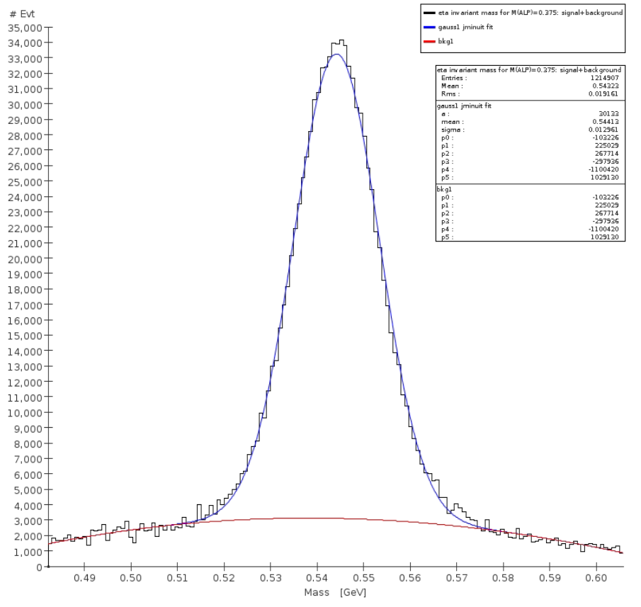
Figure 67: Invariant mass of $\eta\rightarrow\gamma\mu^{+}\mu^{-}$ for for 4.5 $\times 10^{14}$ POT. The plot includes the Urqmd generated background. See text for an explanation of the fitting procedure.

The reconstruction efficiency for the various steps of the analysis, along with the final branching ratio sensitivity extracted with the analysis, are summarized in Table 35.

Process	Trigger	Trigger	Trigger	Reconstruction		Total	Branching ratio
	L0	L1	L2	+ analysis			sensitivity
$\eta\rightarrow\gamma\mu^{+}\mu^{-}$	80.6%	64.6%	94.3%	$92.9$%		$45.6$%	$1.93\times 10^{-9}\pm 0.9\times 10^{-11}$
Urqmd	$21.7\%$	$1.7\%$	$22.2\%$	$4.7\times 10^{-3}$%		$4.7\times 10^{-6}$%	-

Table 35: Reconstruction efficiencies for $\eta\rightarrow\gamma\mu^{+}\mu^{-}$and for the Urqmd background. Errors are statistical only and are obtained assuming 4.5 $\times 10^{14}$ POT.

The sensitivity to the Wilson coefficients is derived for the longitudinal asymmetry, see Ref. Sanchez-Puertas (2019), that will be limited by statistical error on the signal diluted by the background. The values are obtained from Table 35 for 4.5$\times 10^{14}$ POT, and scaled for the total luminosity foreseen at REDTOP.

Combining them, we expect for the statistical error $\Delta(A_{L})$ of the asymmetry:

$$\Delta(A_{L})=\frac{\sqrt{N}_{\textrm{$\eta\to\gamma\mu^{+}\mu^{-}$}}+\sqrt{N}_{\textrm{bkg}}}{N_{\textrm{$\eta\to\mu^{+}\mu^{-}$}}}.$$ (121)

Taking the expected $\eta$ and background events from Table 23 and the efficiencies above, we obtain $N_{\eta\to\gamma\mu^{+}\mu^{-}}=N_{\eta}\times\textrm{BR}(\eta\to\gamma\mu^{+}\mu^{-})\times\epsilon_{\textrm{reco}}\times\epsilon_{\textrm{pol}}$, together with $N_{\textrm{bkg}}=N_{ni}\times\epsilon_{\textrm{reco}}\times\epsilon_{\textrm{pol}}$. Assuming a conservative $\epsilon_{\textrm{pol}}=50\%$ estimate both for signal and background, we obtain $\Delta(A_{L})=1.4\times 10^{-5}$. Comparing to the longitudinal asymmetries defined in Ref. Sanchez-Puertas (2019), one could achieve, for the Wilson coefficients responsible for the asymmetries, the following sensitivity:

$$\Delta(c_{\ell equ}^{1122})=2.6,\quad\Delta(c_{\ell edq}^{1122})=2.6,\quad\Delta(c_{\ell edq}^{2222})=1.7.$$ (122)

XIII.5 CP- violation studies from the asymmetry of the decay planes of $\eta\rightarrow\mu^{+}\mu^{-}e^{+}e^{-}$

Testing $CP$-violation in pseudoscalar mesons via a search for asymmetries in double Dalitz decay has the advantage that it does not require to measure the polarization of the leptons. A recent theoretical model (Sanchez-Puertas, 2019) assumes that the asymmetry in this process arises from heavy physics. As a consequence, the Standard Model effective field theory (SMEFT) can be applied to relate the Wilson coefficients (carrying the CP-violating parameters) and the observable quantities. A detailed discussion of that model can be found in Sec. III.2.5.

The sensitivity to $CP$-violation is explored by examining the following two asymmetries:

$$A_{sin\Phi cos\Phi}=\frac{N(\sin\phi\cos\phi>0)-N(\sin\phi\cos\phi<0)}{N(\sin\phi\cos\phi>0)+N(\sin\phi\cos\phi<0)}$$ (123)

$$A_{sin\Phi}=\frac{N(\sin\phi>0)-N(\sin\phi<0)}{N(\sin\phi>0)+N(\sin\phi<0)}$$ (124)

where $\phi$ is the angle between the decay planes of the $e^{+}e^{-}$ and the $\mu^{+}\mu^{-}$ pairs (see also Fig. 63). The reason for probing different asymmetries is due to the fact that they are proportional to different operators. More specifically, amongst all the possible invariants describing the 4-body kinematics ($A4-A8$, see, for example, Appendix A in Kampf et al. (2018):), it is only $A8$, proportional to $sin(\phi)$, that changes sign under $P$ (while it is even under $C$). Of course, $A8$ might come accompanied by additional invariants, such as $A7$, that would produce an overall asymmetry also in $sin(\phi)cos(\phi)$.

Several events sets, each corresponding to 7.4$\times 10^{13}$ POT (or $2.4\times 10^{9}$ $\eta$-mesons), were generated with $GenieHad$ with $<sign(sin(\phi)cos(\phi)>$ ranging from 0 to $4\times 10^{-2}$ and $<sign(sin(\phi)>$ ranging from 0 to $4\times 10^{-2}$. The full chain of generation-simulation-reconstruction-analysis was repeated for each event set. The largest background for this final state originates from the decays $\eta\rightarrow\pi^{+}\pi^{-}\pi^{0}$ and $\eta\rightarrow\pi^{+}\pi^{-}\gamma$ followed by $\gamma\rightarrow e^{+}e^{-}$ and $\pi^{0}\rightarrow\gamma e^{+}e^{-}$, where both pions where mis-identified as muons. Another important source of background is due to the combinatorics from two mis-identified charged pions, generated by nuclear interaction of the beam on the target, and from a spurious photon, usually generated from the decay of a $\pi^{0}$ or $\eta$ meson, which then converts in the materials of the detector. The excellent particle identification of REDTOP keep such background to a very low levels, as shown in Table 36. Very generic requirements on the quality of reconstructed particles were applied to the signal and background samples. Neutral pions, decaying into $\gamma e^{+}e^{-}$ and $\gamma\gamma$, where reconstructed by considering all combinations of photons, electrons and positrons with an invariant mass within 5 MeV from $\pi^{0}$ mass. This requirement is able to reject most of the combinatoric background, where no $\eta$ mesons are present in the final state. Similarly, photons converting into a $e^{+}e^{-}$ pair where reconstructed by requiring that the invariant mass of the $e^{+}e^{-}$ pair was lower than 5 MeV.

The average reconstruction efficiency for all signal sets and for the Urqmd background is summarized in Table 36 along with the sensitivity to the branching ratio obtained by using Eq. 105 for $3.3\times 10^{18}$ POT.

Process	Benchmark	Trigger	Trigger	Trigger	Reco	Analysis	Total
	set	L0	L1	L2
$\eta$$\rightarrow\mu^{+}\mu^{-}e^{+}e^{-}$	average.	$80.4$%	$57.0$%	$20.4$%	$16.6$%	$58.2$%	$0.9$%
Urqmd		$21.7\%$	$1.7\%$	$22.2\%$	$1.0\times 10^{-4}$%	$36.4$%	$3.0\times 10^{-8}$%

Table 36: Reconstruction efficiencies for $\eta\rightarrow\mu^{+}\mu^{-}e^{+}e^{-}$ final state and for the Urqmd generated background. The values are averaged over the benchmark sets.

The invariant mass of the $\mu^{+}\mu^{-}e^{+}e^{-}$ systems for the events surviving the cuts is shown in Fig. 68. The combinatorics background is nicely fitted under the $\eta$ peak.

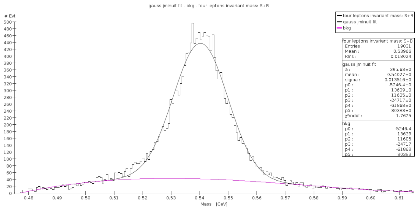
Figure 68: Invariant mass of the $\mu^{+}\mu^{-}e^{+}e^{-}$ system. The plot includes the Urqmd generated background. See text for an explanation of the fitting procedure.

The data for each event set were divided into separate $sin\varphi cos\varphi$>0 and $sin\varphi cos\varphi<0$ groups and $sin\varphi$>0 and $sin\varphi<0$. The $\eta$ content in each group was extracted from a fit to the sum of a Gaussian function and a 5th-order polynomial and by integrating the Gaussian signal after background subtraction. The asymmetries extracted with such procedure are plotted in Fig. 69 vs the Monte Carlo generated value. The diluting effect of the background on the asymmetry is much reduced compared to the $\eta\rightarrow\pi^{+}\pi^{-}e^{+}e^{-}$ case. In fact, almost no degradation can be observed. We conclude that the measured asymmetry for the samples considered is larger than the statistical error (which is the dominant component in previous measurements by WASA and KLOE experiments) for values of the true asymmetry larger than approximately $1\times 10^{-2}$. When extrapolating the results to the full integrated luminosity of $3.3\times 10^{18}$ POT foreseen for REDTOP, we estimate that the statistical error will be reduced by about than two orders of magnitude, corresponding to a contribution to the sensitivity smaller than $\simeq 10^{-4}$. Therefore, we conclude that the uncertainty on the measured asymmetry will, most likely, be dominated by the systematic error.

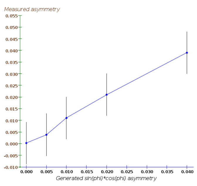
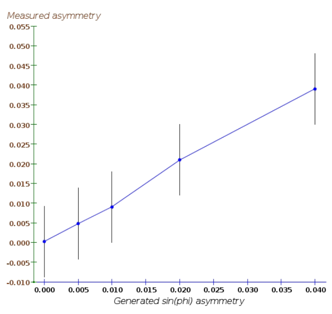
Figure 69: Sensitivity to $sin\varphi cos\varphi$ (left) and $sin\varphi$ (right) asymmetries for $\eta\rightarrow\mu^{+}\mu^{-}e^{+}e^{-}$.

Using the results in Sec. III.2.5, we obtain the following sensitivities for the full integrated luminosity

$$\Delta c_{\ell edq}^{2222}=8,\quad\Delta c_{\ell edq}^{2222}=5,\quad\Delta\epsilon_{1}=5\times 10^{-4},\quad\Delta\epsilon_{2}=0.3.$$ (125)

XIII.6 CP-violation studies in the decay $\eta\rightarrow\pi^{0}\mu^{+}\mu^{-}$

A detailed discussion on probing CP-violation in semi-leptonic $\eta$ decays can be found in Sec. III.2.6 along with the relationship between the Wilson coefficients (carrying the CP-violating parameters) and the observable quantities.

The sensitivity to this process is studied by measuring the polarization of the muon reconstructed from the following process:

• $p+Li\rightarrow\eta+X\;with\;\eta\rightarrow\pi^{0}\mu^{+}\mu^{-}$

The two relevant observables are the two asymmetries defined in Eqs.(81,82), that carry the information from the muon polarization. The event generation for this process is based on the model described in Sec. III.2.6. A sample consisting of $\sim 2.3\times 10^{8}$ $\eta$ mesons from 7$\times$$10^{12}$ POT (corresponding to 2$\times$$10^{-6}$ of the integrated luminosity foreseen for the experiment). The full chain of generation-simulation-reconstruction-analysis for this process follow closely that described in Sec. X.3 since the final states considered for the two analyses are, essentially, the same. The invariant mass of the reconstructed $\pi^{0}\mu^{+}\mu^{-}$ system was fitted using the sum of a Gaussian and a 5th-order polynomial. The integral of the fit function was used to extract the branching ratio sensitivity for this process.

The reconstruction efficiency for the various steps of the analysis, along with the resulting branching ratio sensitivity are summarized in Table 37.

Process	Trigger	Trigger	Trigger	Reconstruction		Total	Branching ratio
	L0	L1	L2	+ analysis			sensitivity
$\eta\rightarrow\pi^{0}\mu^{+}\mu^{-}$	64.1%	36.7%	91.4%	$73.2$%		$15.7$%	$9.4\times 10^{-9}\pm 1.3\times 10^{-10}$
Urqmd	$21.7\%$	$1.7\%$	$22.2\%$	$1.6\times 10^{-2}$%		$1.3\times 10^{-5}$%	-

Table 37: Reconstruction efficiencies for $\eta\rightarrow\pi^{0}\mu^{+}\mu^{-}$and for the Urqmd background. Errors are statistical only and are obtained assuming 7$\times 10^{12}$ POT.

The sensitivity to the Wilson coefficients is derived through the most sensitive asymmetry, Eq. (81), that will be limited by statistical error on the signal diluted by the background. The values are obtained from Table 37 for 7.2$\times 10^{12}$ POT, after scaling for the total integrated luminosity foreseen for REDTOP (cf. Table 23.

Combining them, we expect for the statistical error:

$$\Delta(A_{L})=\frac{\sqrt{N}_{\textrm{$\eta\to\pi^{0}\mu^{+}\mu^{-}$}}+\sqrt{N}_{\textrm{bkg}}}{N_{\textrm{$\eta\to\mu^{+}\mu^{-}$}}}.$$ (126)

Taking: $N_{\eta\to\pi^{0}\mu^{+}\mu^{-}}=N_{\eta}\times\textrm{BR}(\eta\to\pi^{0}\mu^{+}\mu^{+})\times\epsilon_{\textrm{reco}}\times\epsilon_{\textrm{pol}}=1.0\times 10^{4}$, with $N_{\eta}=1.1\times 10^{14}$ , $\textrm{BR}=1.2\times 10^{-9}$ Escribano and Royo (2020) $\epsilon_{\textrm{reco}}=15.7$% , $N_{bkg}=1.3\times 10^{-7}\times.5\times 10^{16}\times\epsilon_{\textrm{pol}}$=1.6$\times$10⁹, $\epsilon_{\textrm{pol}}=50\%$ for the $\mu^{\pm}\rightarrow e^{\pm}\nu\overline{\nu}$ decay, we obtain: $\Delta(A_{L})=4.0$. Comparing to Eq. (81), we find, for the Wilson coefficients responsible for the asymmetries, the following sensitivity:

$$\Delta(c_{\ell equ}^{1122})=21,\quad\Delta(c_{\ell edq}^{1122})=21,\quad\Delta(c_{\ell edq}^{2222})=200.$$ (127)

XIII.7 Lepton flavor violation in the decay $\eta\rightarrow e^{+}\mu^{-}$+ c.c.

This study requires the reconstruction of an electron/positron and a muon in the final state. It is especially challenging since a pion has a non-null probability to fake a muon. Considering the large number of pions generated in the proton-target scattering, we expect that the sensitivity to measure the branching ratio for this process is considerably lower than all others considered so far.

A sample consisting of $\sim 8.6\times 10^{9}$ $\eta$ mesons from 2.6$\times$$10^{14}$ POT (corresponding to 7.8$\times$$10^{-5}$ of the full integrated luminosity foreseen for the experiment). The full chain of generation-simulation-reconstruction-analysis described in Sec. VII.4 was repeated for each event set. Very generic requirements on the quality of reconstructed particles were applied to the signal and background samples. The main background for this channel is due to the non-resonant decay $\eta\rightarrow\gamma\mu^{+}\mu^{-}$ which occurs with a relatively large branching ratio of $3.1\times 10^{-4}$ occurring in the presence of a gamma conversion: $\gamma\rightarrow e^{+}e^{-}$. The second largest background contribution originates from charged pions mis-identified as muons. With the present detector layout, the $\pi$/$\mu$ mis-identification probability was estimates to be $\sim$3.5%. In order to reduce such background, we imposed the requirement that no photons should be detected in the calorimeter.

Neutral pions, decaying into $\gamma e^{+}e^{-}$ and $\gamma\gamma$, where reconstructed by considering all combinations of photons, electrons and positrons with an invariant mass within 5 MeV from $\pi^{0}$ mass. Similarly, photons converting into a $e^{+}e^{-}$ pair where reconstructed by requiring that the invariant mass of the $e^{+}e^{-}$ system was lower than 5 MeV. Reconstructed $\pi^{0}$ ’s and $\gamma$’s were removed from the event. Finally, the events were required to have a topology consistent with a $\eta\rightarrow e^{\pm}\mu^{\mp}$ final state, and an invariant mass compatible with the $\eta$ mass.

The reconstruction efficiencies for this process and for the Urqmd background is summarized in Table 38. For illustrative purposes, Fig. 70 shows the fit to the invariant mass of the reconstructed $e^{\pm}\mu^{\mp}$ system along with the Urqmd generated background, assuming BR($\eta\rightarrow e^{\pm}\mu^{\mp}$)= $1.4\times 10^{-4}$ and an $\eta$ sample of $5\times 10^{8}$ (corresponding to $4.5\times 10^{-6}$ of the full integrated luminosity). The number of reconstructed signal and background events was obtained form a fit to the $\eta$ meson invariant mass using the sum of a Gaussian and a 5th-order polynomial. The integral of the fitted function is used to extract the branching ratio for this process.

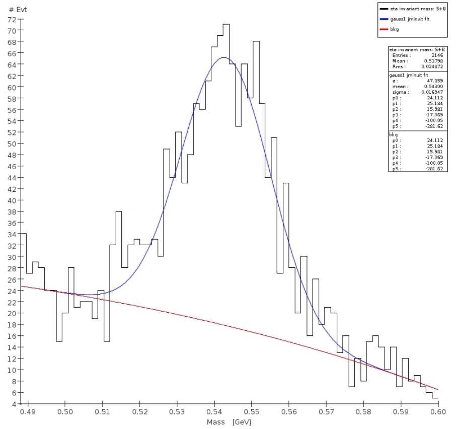
Figure 70: Invariant mass of $e^{+}\mu^{-}$ + c.c . The plot includes the Urqm generated background. See text for an explanation of the fitting procedure.

The resulting branching ratio sensitivity is summarized in Table 38.

Process	Trigger	Trigger	Trigger	Reco		Total	Branching ratio
	L0	L1	L2				sensitivity
$\eta\rightarrow e^{+}\mu^{-}+c.c.$	$79.3$	$21.3\%$	$89.7\%$	$14.0\%$		$2.1$%	$1.4\times 10^{-7}\pm 2\times 10^{-9}$
Urqmd	$21.7\%$	$1.7\%$	$22.2\%$	$0.01$%		$8.2\times 10^{-6}$%

Table 38: Reconstruction efficiencies for $\eta\rightarrow e^{+}\mu^{-}+c.c.$ and for the Urqmd generated background

XIII.7.1 Concluding remark

As stressed above, the reconstruction of the process $\eta\rightarrow e^{+}\mu^{-}+c.c.$ suffers from a large combinatorics background due to misidentified pions generated in the target by the primary proton and gamma converting in the fiber tracker. The excellent 4-momentum resolution of the detector only partially mitigate this problem. From the study performed, we conclude that the tagging of the $\eta$ meson could considerably improve the branching ratio sensitivity, as most of the combinatorics background could be identified and rejected. Another improvement would arise from reducing the material budget in the vertex detector, where the gamma conversion is reconstructed with lower efficiency. In that respect, the adoption of the ITS3 option (cf. Sec. VI.4.1) would be, in fact, an attractive solution.

XIII.8 Test of Lepton Flavor Universality

Leptonic and semileptonic decays of the $\eta$ mesons have relatively clear signatures in REDTOP, and they can be disentangled with good efficiency, from the large hadronic background. Furthermore, the decay rate into electrons and muons are only slightly affected by the different phase space. Therefore, those decays represent an excellent opportunity to probe Lepton Flavor Universality (LFU). In this work, we have considered two groups of processes: $\eta\to\ell_{1}\bar{\ell}_{1}\ell_{2}\bar{\ell}_{2}$, and $\eta\to\gamma\ell\bar{\ell}$.

XIII.8.1 $\eta\rightarrow 4\>leptons$ decays

These constitute yet another set of interesting decays. Within the SM, these decays include $\eta^{(\prime)}\to\ell_{1}\bar{\ell}_{1}\ell_{2}\bar{\ell}_{2}$, where $\ell_{i}$ can be either of $e$ or $\mu$. Interestingly, the amplitude for these decays is dominated by the very same dynamics—the $\eta^{(\prime)}\to\gamma\gamma$ vertex—that also describes the decays to two leptons, discussed in Sec. III.2.8. In the case of 4 leptons, both the photons are off-shell and produce $\ell\bar{\ell}$ pairs (“Dalitz pairs”). It is interesting that, although all of the decay channels $e\bar{e}$, $e\bar{e}\gamma$, $\mu\bar{\mu}$, $\mu\bar{\mu}\gamma$, and $\ell_{1}\bar{\ell}_{1}\ell_{2}\bar{\ell}_{2}$ all probe the very same underlying form factor, the different decays entail somewhat different “effective dilepton masses” and thereby probe this form factor in somewhat different kinematic regions for the off-shell photons. In practice, the contributions from large “effective masses” are negligible in the $e\bar{e}$ case, hence e.g. the $\eta^{(\prime)}\to e\bar{e}e\bar{e}$ and $\eta^{(\prime)}\to e\bar{e}\mu\bar{\mu}$ cases can usefully be inferred from the $\eta^{(\prime)}\to e\bar{e}$ and $\eta^{(\prime)}\to\mu\bar{\mu}$ ones Jarlskog and Pilkuhn (1967). Besides, the contribution from non-zero $k_{1,2}^{2}\neq 0$ ($k_{i}$ denoting the photon momenta in the $\eta^{(\prime)}\to\gamma\gamma$ vertex) are actually in the ballpark of 30% in the muon case Jarlskog and Pilkuhn (1967). In the presence of LFV New Physics, one may add to the above decays the further channels $\eta^{(\prime)}\to\ell_{1}\bar{\ell}_{2}\ell_{2}\bar{\ell}_{2}$, where again $\ell_{i}$ can be either of $e$ or $\mu$. Considering for definiteness the LQ case already discussed in Sec. III.2.8 the underlying diagrams for these channels are similar: $t$-channel LQ exchange, further radiating an off-shell photon. Then the LQ vertices yield two oppositely charged leptons of different flavour, and the photon produces the two remaining like-flavoured leptons. Hence we see that, as is the case for the SM amplitude, also the NP amplitude is—for the 2-lepton and 4-lepton cases alike—dominated by the very same building block. In the presence of abundant data, a joint analysis of all channels is thus warranted. As already mentioned earlier, the NP amplitude tends to be sensitive to light NP, not exceeding $\sim 20$ GeV.

A detailed discussion on possible ways to probe Lepton Universality $\eta^{(\prime)}\to\ell_{1}\bar{\ell}_{1}\ell_{2}\bar{\ell}_{2}$, where $\ell_{i}$ can be either of $e$ or $\mu$ can be found in Sec. III.2.8.

Only the decays of the $\eta\rightarrow e^{+}e^{-}e^{+}e^{-}$ has been experimentally observed, with a measured branching ratio of $2.4\times 10{}^{-5}$  (Zyla et al., 2020b), corresponding to an expected yield at REDTOP of $2.6\times 10^{9}$ produced events. An estimate for the other two processes can be made following Ref. (Kampf et al., 2018), for which we foresee a yield of order $\mathcal{O}(10^{7})$ and $\mathcal{O}(10^{4})$, respectively, for the $\eta\rightarrow e^{+}e^{-}\mu^{+}\mu^{-}$ and $\eta\rightarrow\mu^{+}\mu^{-}\mu^{+}\mu^{-}$ decays. The studies performed on these processes have been carried using different $\eta$-meson samples. The corresponding POT are summarized in the second column of Table 40. The full chain of generation-simulation-reconstruction-analysis was repeated for each event set. Very generic requirements on the quality of reconstructed particles were applied to the signal and background samples. The final states with muons are relatively background free, as the combinatorics can hardly mimic the PID and kinematics of the signal.

The main background for the $\eta\rightarrow e^{+}e^{-}e^{+}e^{-}$ channel is due to the non-resonant decay $\eta\rightarrow\gamma e^{+}e^{-}$ which occurs with a relatively large branching ratio of $3.1\times 10^{-4}$, accompanied by the gamma conversion: $\gamma\rightarrow e^{+}e^{-}$. The second largest background contribution originates from events with multiple neutral pions decaying as: $\pi^{0}\rightarrow\gamma e^{+}e^{-}$.

In order to reduce the combinatoric background, neutral pions, decaying into $\gamma e^{+}e^{-}$ and $\gamma\gamma$, where reconstructed by considering all combinations of photons, electrons and positrons with an invariant mass within 5 MeV from $\pi^{0}$ mass. Similarly, photons converting into a $e^{+}e^{-}$ pair where reconstructed by requiring that the invariant mass of the $e^{+}e^{-}$ system was lower than 5 MeV. Reconstructed $\pi^{0}$ ’s and $\gamma$’s were removed from the event. Finally, the events were required to have a topology consistent with a $\eta^{(\prime)}\to\ell_{1}\bar{\ell}_{1}\ell_{2}\bar{\ell}_{2}$ in the final state, and an invariant mass compatible with the $\eta$ mass.

The reconstruction efficiencies for the three processes and for the Urqmd generated background are summarized in Table 39

Process	Trigger	Trigger	Trigger	Reconstruction	Analysis	Total
	L0	L1	L2
$\eta$$\rightarrow e^{+}e^{-}e^{+}e^{-}$	$96.1\%$	$80.7\%$	$15.5\%$	$63.3$%	$61.2$%	$4.5$%
$\eta\rightarrow e^{+}e^{-}\mu^{+}\mu^{-}$	$80.4$%	$57.0$%	$20.4$%	$16.6$%	$52.8$%	$0.8$%
$\eta\rightarrow\mu^{+}\mu^{-}\mu^{+}\mu^{-}$	$45.1$%	$31.9$%	$25.5$%	$61.3$%	$40.5$%	$0.9$%
Urqmd	$21.7\%$	$1.7\%$	$22.2\%$	$0.9-8.2\times 10^{-4}$%	17.6%-$30.7$%	$0.7-6.7\times 10^{-7}$%

Table 39: Reconstruction efficiencies for $\eta\rightarrow 4\>leptons$ and for the Urqmd generated backgrounds

The number of reconstructed signal and background events was obtained form a fit to the invariant mass of the four leptons, using the sum of a Gaussian and a 5th-order polynomial. The integral of the fitted function is used to extract the branching ratio for the considered process. Fig. 71 shows the invariant mass distribution of the four leptons, along with the fitting curve. The statistical errors obtained from the fit to each final state are summarized in Table. 40.

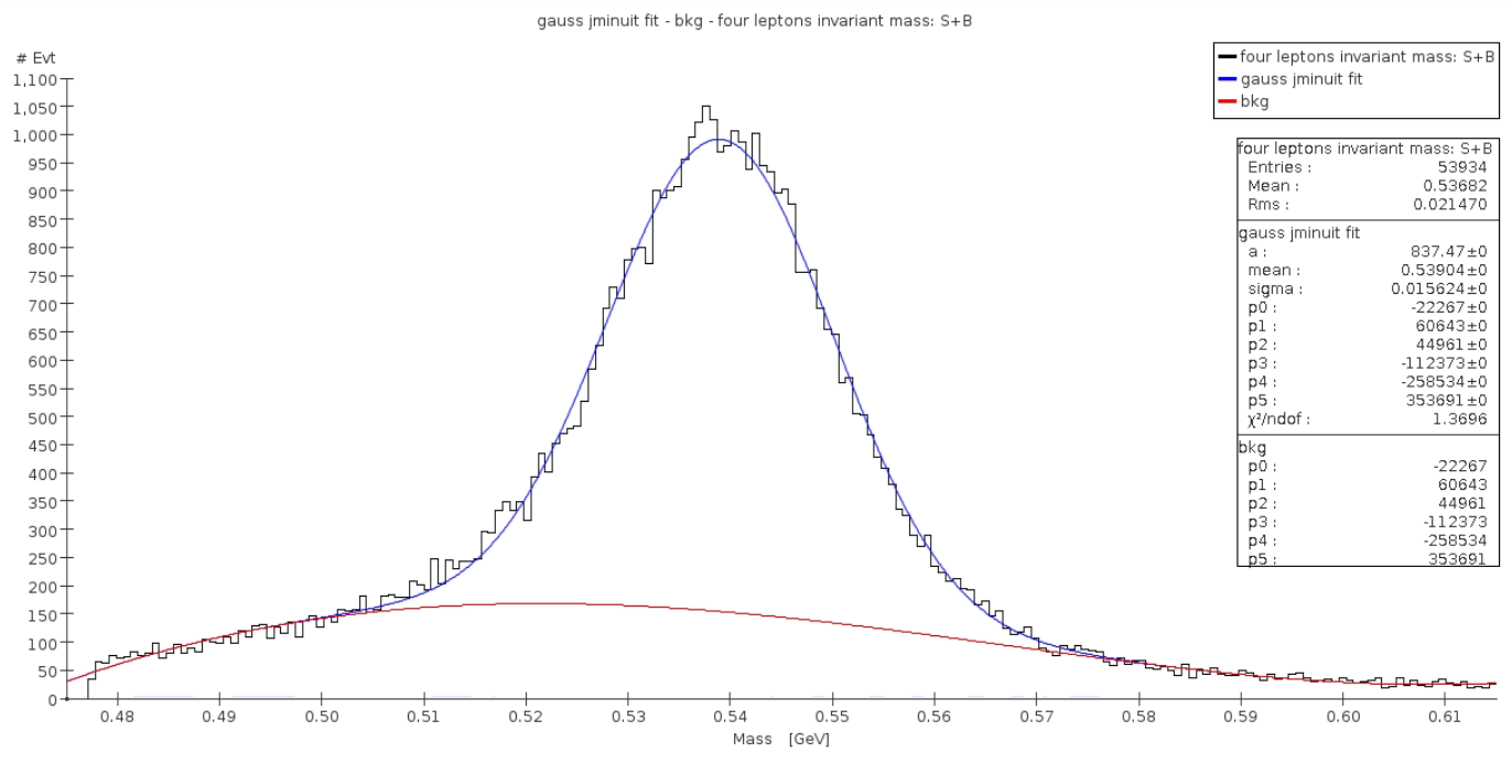
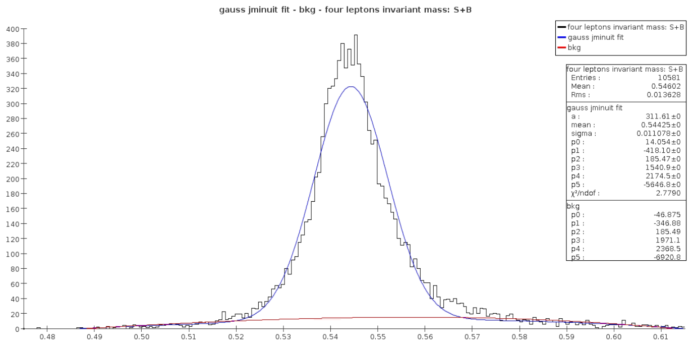
Figure 71: Invariant mass for f $\eta\rightarrow 4\>leptons$ and for the Urqmd generated background for the POT indicated in Table 40. $\eta\rightarrow e^{+}e^{-}e^{+}e^{-}$ (top left), $\eta\rightarrow e^{+}e^{-}\mu^{+}\mu^{-}$(top right) and $\eta\rightarrow\mu^{+}\mu^{-}\mu^{+}\mu^{-}$(bottom).

Process	POT	Signal events	Statistical error
$\eta$$\rightarrow e^{+}e^{-}e^{+}e^{-}$	$4.4\times 10^{14}$	53,934	0.5%
$\eta\rightarrow e^{+}e^{-}\mu^{+}\mu^{-}$	$1.6\times 10^{15}$	18,841	0.8%
$\eta\rightarrow\mu^{+}\mu^{-}\mu^{+}\mu^{-}$	$2.2\times 10^{18}$	10,548	1.0%

Table 40: Statistical error from the fit of $\eta\rightarrow 4\>leptons$ and Urqmd generated background using a gaussian and a 5th-order polynomial. The POT corresponding to each data sample is indicated in the second column.

When the statistics of the full event sample is taken into account, the projected statistical error for the three processes considered here is expected to be of the order of $10^{-5}$.

XIII.8.2 Test of Lepton Flavor Universality with $\eta\rightarrow\gamma\>2\>leptons$ decays

From a theoretical point of view, similar considerations hold as in the case of 2 leptons discussed in Sec. III.2.8. The presence of the additional photon implies additional SM contributions, but the main conclusions reached in the purely leptonic case still hold. One important feature of the radiative 2-leptons case with respect to the non-radiative counterpart is the fact that the chiral suppression inherent in the latter decay Jarlskog and Pilkuhn (1967) is lifted because of the additional photon. Ratios of radiative di-leptonic decay rates, where the numerator and the denominator only differ by the lepton flavour are then excellent tests of Lepton Universality Guadagnoli et al. (2016), and, by the previous argument, they are expected to be very close to unity within the Standard Model.

The studies performed on these processes are based on a relatively small $\eta$-meson sample consisting of 4.65 $\times 10^{6}$ events. That sample corresponds to $\sim 4.2\times 10^{-8}$ of the integrated luminosity foreseen for the experiment. The full chain of generation-simulation-reconstruction-analysis was repeated for each set of the parameters and for the parameters corresponding to the Standard Model prediction. final state. Very generic requirements on the quality of reconstructed particles was applied to the signals and background samples.

In order to reduce the combinatoric background, neutral pions, decaying into $\gamma e^{+}e^{-}$ and $\gamma\gamma$, where reconstructed by considering all combinations of photons, electrons and positrons with an invariant mass within 5 MeV from $\pi^{0}$ mass. Similarly, photons converting into a $e^{+}e^{-}$ pair where reconstructed by requiring that the invariant mass of the $e^{+}e^{-}$ system was lower than 5 MeV. Reconstructed $\pi^{0}$ ’s and $\gamma$’s were removed from the event. Finally, the events were required to have a topology consistent with a $\eta\rightarrow\gamma e^{+}e^{-}$ or $\eta\rightarrow\gamma\mu^{+}mu^{-}$ final states, and an invariant mass compatible with the $\eta$ mass.

The reconstruction efficiencies for the two processes and for the Urqmd generated background are summarized in Table 41

Process	Trigger	Trigger	Trigger	Reconstruction		Total
	L0	L1	L2	& analysis
$\eta$$\rightarrow\gamma\,e^{+}e^{-}$	$80.6\%$	$64.6\%$	$94.3\%$	$92.8$%		$45.6$%
$\eta\rightarrow\gamma\,\mu^{+}\mu^{-}$	$63.2$%	$42.1$%	$90.6$%	$79.1$%		$20.2$%
Urqmd	$21.7\%$	$1.7\%$	$22.2\%$	$1.1\times 10^{-1}$%$\>($$1.64\times 10^{-3}$%)		$9.0\times 10^{-6}$%$\>($$1.3\times 10^{-7}$%)

Table 41: Reconstruction efficiencies for $\eta\rightarrow\gamma\,\>lepton-antilepton$ and for the Urqmd generated background (values in parentheses are for the $\eta\rightarrow\gamma\,\mu\,\mu$ final state).

The number of reconstructed signal and background events was obtained form a fit to the invariant mass of the four leptons, using the sum of a Gaussian and a 5th-order polynomial. The integral of the fitted function is used to extract the branching ratio for the considered process. Fig. 72 shows the invariant mass distribution of $\gamma\,\>lepton-antilepton$, with the fitting function superimposed.

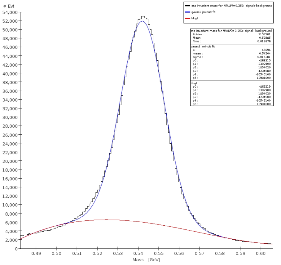
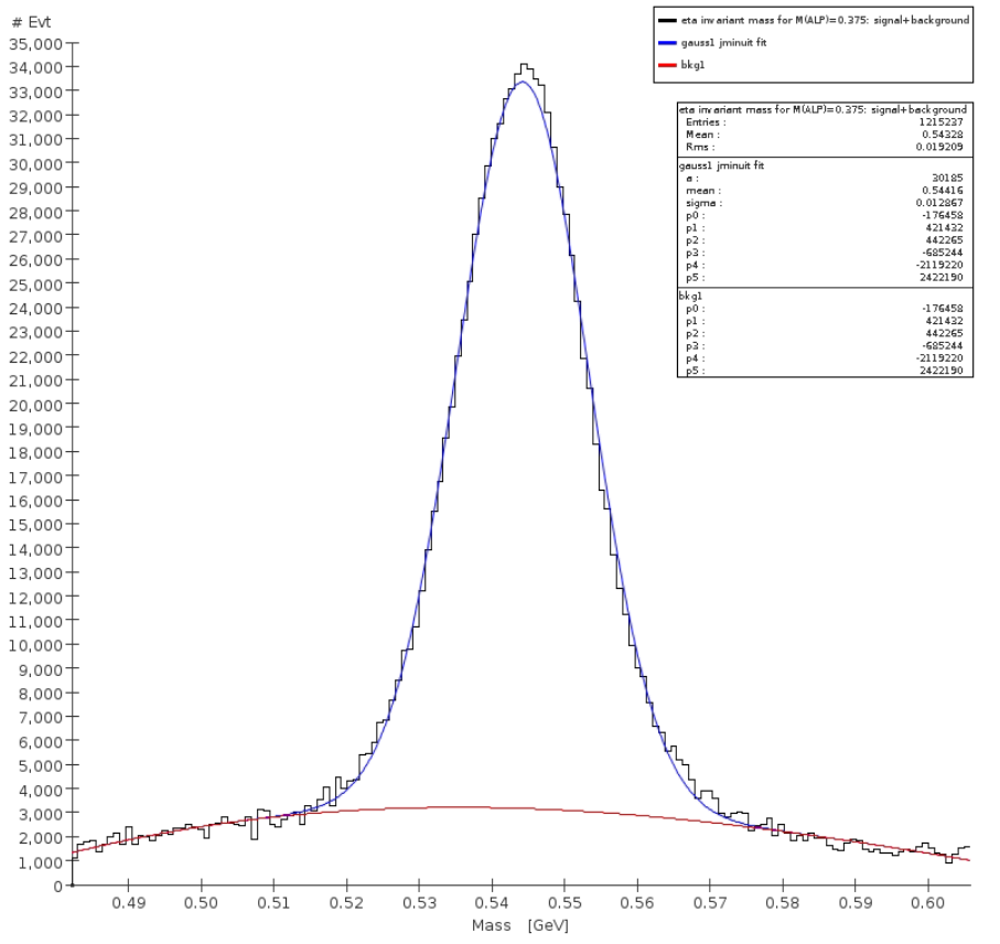
Figure 72: Invariant mass for $\eta\rightarrow\gamma\>lepton-antilepton$ and for the Urqmd generated background.

The statistical errors from the fit to each final state are summarized in Table. 42

Process	POT	Signal events	Background events	$\frac{S}{\sqrt{B}}$	Statistical error
$\eta$$\rightarrow\gamma\,e^{+}e^{-}$	$1.38\times 10^{11}$	$2.13\times 10^{6}$	$2.52\times 10^{4}$	$1.3\times 10^{4}$	0.09%
$\eta\rightarrow\gamma\,\mu^{+}\mu^{-}$	$1.38\times 10^{11}$	$8.84\times 10^{5}$	$6.5\times 10^{3}$	$3.5\times 10^{3}$	0.14%

Table 42: Statistical error from the fit of $\eta\rightarrow\gamma\,\>lepton-antilepton$ and Urqmd generated background using a gaussian and a 5th-order polynomial, for 1.38$\times 10^{18}$ POT

When the statistics of the full event sample for 3.3$\times 10^{18}$ POT is taken into account, the projected statistical error for the $\eta\rightarrow\gamma\,\>lepton-antilepton$ final state is expected to be of the order of $10^{-6}$, certainly negligible compared to the systematic error.

XIII.8.3 Remarks on LFU measurements with $\eta$ mesons

The theoretical discussion about the REDTOP sensitivity to LFU measurements deserves some further qualifications. As well-known, LFU measurements have recently come to the fore because of a coherent array of discrepancies in measurements of semi-leptonic $b\to s$ and $b\to c$ decays at LHCb and $B$ factories. The natural question for the present document is whether the putative beyond-SM LFU that these discrepancies imply could be tested in decays of light mesons, e.g. kaons Alves Junior et al. (2019), and the $\eta^{(\prime)}$. On the latter there is a conspicuous gap in the literature, and on the other hand this possibility would be an important physics case for REDTOP. A positive answer to the question rests on addressing two challenges, that we would like to highlight here, and that definitely warrant further investigation.

The first issue is the fact that LHCb and $B$ factories access decays that directly probe—by definition—the operators affected by the putative $B$ anomalies, i.e., 4-fermion structures of the kind $(\bar{s}\Gamma b)(\bar{\ell}\Gamma^{\prime}\ell)$, where $\Gamma,\Gamma^{\prime}$ denote appropriate strings of Dirac matrices, and $\ell$ is any of the charged leptons. Conversely, in the case of $\eta^{(\prime)}$ we access operators with quarks (and leptons) of the light generations only. Relating the different quark sectors requires assumptions on the flavor structure of the couplings, and the suppression is “by default” CKM-like (see e.g. Borsato et al. (2019)).

The second issue is that $\eta^{(\prime)}$ leptonic decays are dominated by the (long-distance) contribution with two intermediate photons, discussed around eq. (83). As a consequence, in order to have sensitivity to new physics, the latter must give a signal unambiguously larger than the uncertainty associated with such long-distance contribution. To this end, either the new-physics coupling must be large enough (but it cannot exceed $\sim 4\pi$), and/or the new-physics mass scale $M$ has to be sufficiently small. As a reference, $Z$-boson exchange yields per-mil modifications of the rate Gan et al. (2022), as already discussed in this document. This makes these decays way more suited as probes of light, MeV–GeV-scale new physics. This happens to be a very active field of research currently (see e.g. Lanfranchi et al. (2021) for a recent review), and has even been considered as a solution of $B$ anomalies Datta et al. (2017); Sala and Straub (2017); Datta et al. (2018); Alok et al. (2017); Altmannshofer et al. (2018); Datta et al. (2019); Darmé et al. (2020, 2021).

The task of pinning down such a possibility is daunting but not hopeless, and definitely worth pursuing given the huge opportunities it would open. Keeping in mind the above issues, the task at hand would be to study different flavour assumptions within an appropriate, general model of the new effects, and perform a joint analysis of the different flavour sectors. Note that the “appropriate model” cannot be the effective-theory framework used in many of the phenomenological interpretations of current $B$ anomalies, because light new physics has to be kept as dynamical degrees of freedom. However, the formalism to address this possibility in a general way exists (see e.g. Arina et al. (2021)). One can thus study systematically the question under which circumstances the shifts to semi-leptonic operators from light new physics that can explain the $B$ anomalies would “spill over” to $\eta^{(\prime)}$ decays. Addressing this question goes clearly outside the scope of this document, but we reiterate its interest and wide applicability.

XIV Sensitivity to Non-perturbative QCD

XIV.1 Form factor studies

The studies on the $\eta$ and $\eta^{\prime}$ transition form factors can be of great importance in the evaluation of the dominant pseudoscalar-exchange contribution to the HLbL scattering contribution to the prediction of the anomalous magnetic moment of the muon, as discussed in Sec.IV. A good precision in the determination of those form factors could unquestionably help in shedding more light on this topic.

A detailed discussion on the $\eta$ form factors with semileptonic decays can be found in Sec. IV. The sensitivity is explored by looking at the kinematics of the di-muon system reconstructed from the following process:

• $p+Li\rightarrow\eta+X\;with\;\eta\rightarrow\gamma\mu^{+}\mu^{-}$

The amplitude for such decay can be written as (cf. Sec. III.2.4):

$$\mathcal{M}=\epsilon^{\mu\nu\rho\sigma}\varepsilon_{\mu}^{*}k_{\nu}q_{\sigma}[\bar{u}(p_{-})\gamma_{\rho}v(p_{+})]F_{\eta\gamma^{*}\gamma^{*}}(q^{2},0)q^{-2}$$ (128)

where $q=p_{+}+p_{-}$ is the sum of the the lepton momenta, $k$ is the photon momenta, and $\varepsilon$ the photon polarization, and $F_{\eta\gamma^{*}\gamma^{*}}(q^{2})$ the transition form factor characterizing the $\eta$ structure. A phenomenologically useful (and simple) parametrization for the form factor is the following (see Sec. IV for details):

$$\tilde{F}_{\eta\gamma^{*}\gamma^{*}}(s,0)=\frac{\Lambda^{2}}{\Lambda^{2}-s}.$$ (129)

where $\Lambda\simeq m_{\rho}\simeq 770$MeV. A recent measurement by A2 Coll. Aguar-Bartolome et al. (2014) was based on of 2.2$\times$10⁴ $\eta\rightarrow\gamma e^{+}e^{-}$ decays from a total of 3$\times$10⁷ $\eta$ mesons produced in the $\gamma\,p\rightarrow\eta\,p$ reaction, resulting in a statistical error on $\varLambda$ of $\sim 8\%$. As discussed in Sec. III.2.4, the $\eta\rightarrow\gamma\mu^{+}\mu^{-}$ channel has larger sensitivity than $\eta\rightarrow\gamma e^{+}e^{-}$.

Five event sets, each consisting of $\sim 3.5\times 10^{5}$ $\eta\rightarrow\gamma\mu^{+}\mu^{-}$ decays where generated with $GenieHad$. That statistics corresponds to 1.1$\times$10⁹ $\eta$ mesons produced, or, $\sim 1\times 10^{-5}$ of the integrated luminosity foreseen for the experiment. The sets where generated with the matrix element described in Sec. III.2.4 and $\varLambda$ ranging from 660 MeV to 800 MeV. One extra sample was generated with a point-like form factor, corresponding to a pure QED process. The distribution of the $\nicefrac{{d\Gamma}}{{ds}}$, where $s$ is the invariant mass squared of the $\mu^{+}\mu^{-}$ system is shown in Fig. 73.

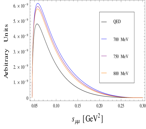
Figure 73: Generated spectrum $\frac{d\varGamma}{ds}$ for $\eta\rightarrow\gamma\mu^{+}\mu^{-}$ (s=$\mid P_{\mu^{+}}+P_{\mu^{-}}\mid^{2}$).

Different values of the parameter $\varLambda$ affect both the shape of distribution as well as the total decay rate of the process.

The analysis oh this final state proceeds according the same guidelines as those performed for the  CP-violation in semileptonic $\eta$ decays(cf. Sec. XIII.4). The full chain of generation-simulation-reconstruction-analysis was repeated for each set of the parameters and for the parameters corresponding to the Standard Model prediction. final state. Very generic requirements on the quality of reconstructed particles was applied to the signals and background samples.

The largest background contribution to this process is found to originate from mis-identified pions, mistakenly reconstructed as muons. In fact, the $\pi$/$\mu$ mis-identification probability for the detector considered in this work has a conservative value of $\simeq 3.5\%$ (or, $\simeq 0.12\%$ for mis-identifying both leptons). Since the probability of generating two charged pions in the primary interaction is almost 11% (see, also, Fig. 17), and the probability of having at least one $\pi^{0}$ is 58%, we expect that about $\sim 1.9\times 10^{11}$ events could potentially fake a $\eta\rightarrow\gamma\mu^{+}\mu^{-}$ process. The second largest background is due to process $\eta\rightarrow\gamma\pi^{+}\pi^{-}$, when both pions are accidentally misidentified as muons and their kinematics is compatible with an invariant mass of a genuine $\eta$ decay.

The reconstruction efficiencies for this channel and for the Urqmd background are summarized in Table 43

Process	Trigger	Trigger	Trigger	Reconstruction	Analysis	Total
	L0	L1	L2
$\eta\rightarrow\gamma\mu^{+}\mu^{-}$	80.6%	64.4%	94.3%	94.2%	98.6%	45.6%
Urqmd	$21.7\%$	$1.7\%$	$22.2\%$	0.014%	47.3%	4.7$\times 10^{-6}$

Table 43: Reconstruction efficiencies for $\eta\rightarrow\gamma\mu^{+}\mu^{-}$ and for the Urqmd generated backgrounds

Fig. 74 shows the invariant mass distribution of the reconstructed particles, fitted with a Gaussian and a 5th-order polynomial.

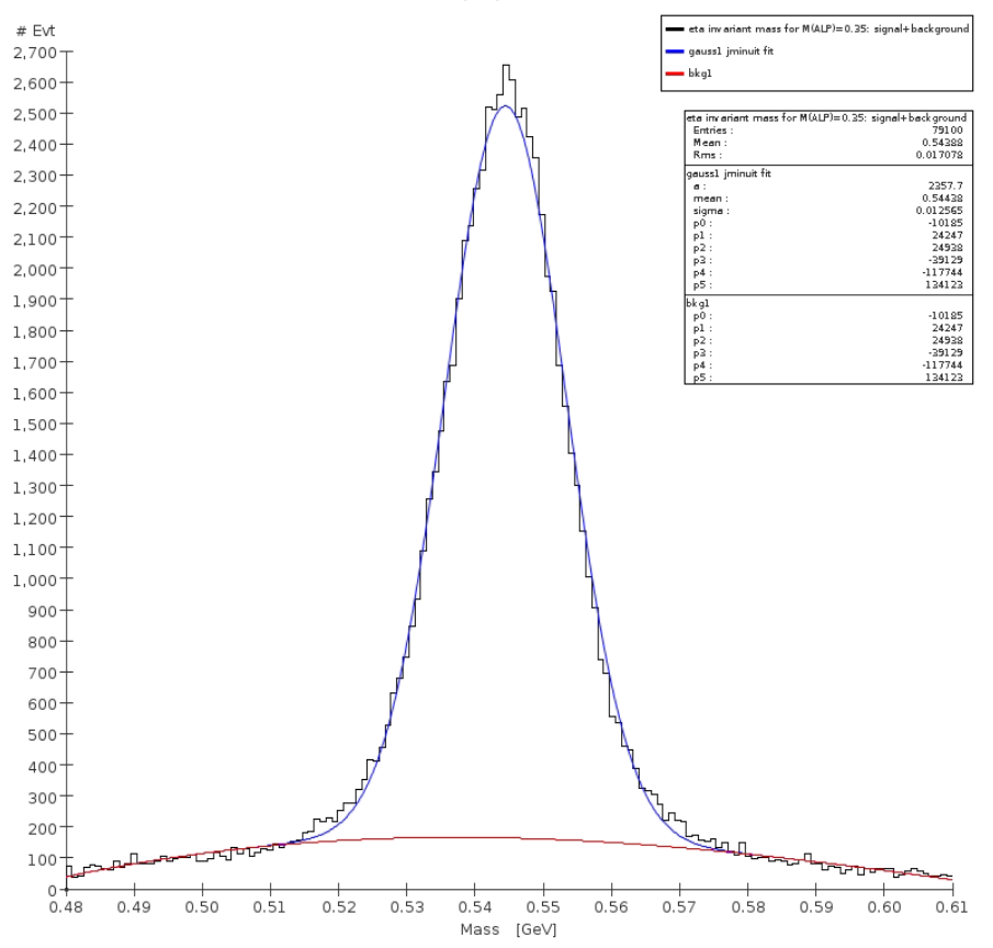
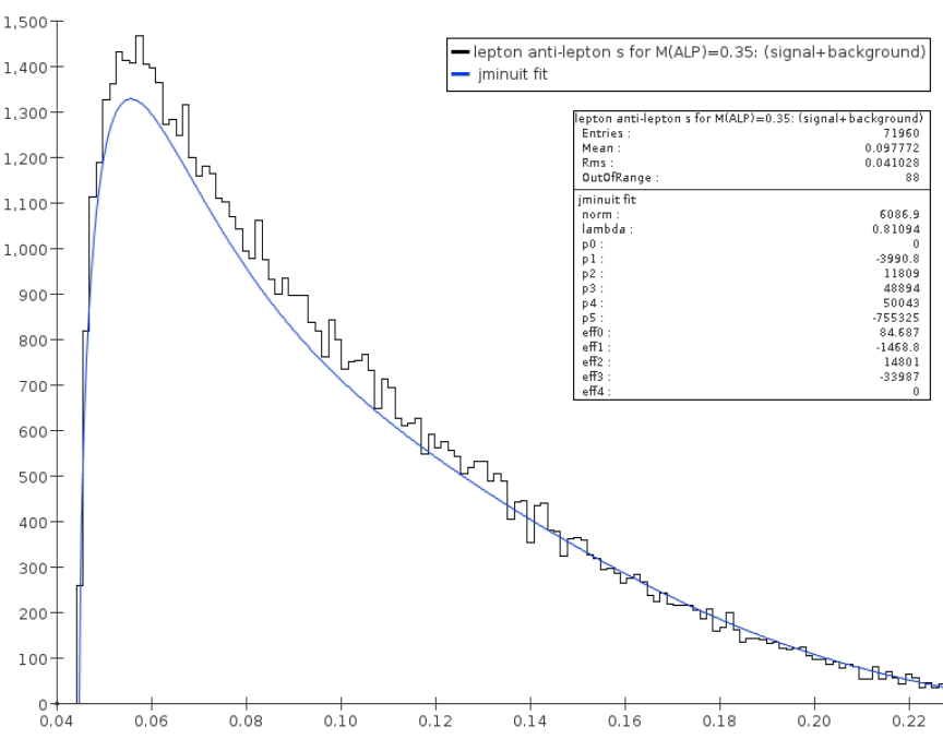
Figure 74: Invariant mass for $\eta\rightarrow\gamma\mu^{+}\mu^{-}$ and for the Urqmd generated background (left) and fit to (s=$\mid P_{\mu^{+}}+P_{\mu^{-}}\mid^{2}$) (right) for the set of events corresponding to $\varLambda=800\,MeV$. See text for an explanation of the fitting procedure.

The sensitivity for the $\varLambda$ parameter is estimated with two different approaches: a) by measuring the branching ratio ; b) by directly fitting the $\frac{d\varGamma}{ds}$ distribution.

Branching ratio method.

In this approach, the uncertainty on the $\varLambda$ parameter is obtained from the fact that: $BR(\eta\rightarrow\gamma\mu^{+}\mu^{-})\propto\mid\tilde{F}_{\eta\gamma^{*}\gamma}(s)\mid^{2}$ and $\varLambda$ controls the value of $BR(\eta\rightarrow\gamma\mu^{+}\mu^{-})$ via the of $\mid\tilde{F}_{\eta\gamma^{*}\gamma}(s)\mid^{2}$ from it. Therefore, the sensitivity on $\mid\tilde{F}_{\eta\gamma^{*}\gamma}(s)\mid^{2}$ is derived by the uncertainty on the measurement of the branching ratio.

The branching ratios and the corresponding statistical errors are obtained from the value of the reconstruction efficiency from the last column of Table 43 and from the fit to the $\gamma\mu^{+}\mu^{-}$invariant mass, as described above. The branching ratios are renormalized to the PDG value and to the central value of the $\varLambda$ parameter measured by the by A2 Coll. Aguar-Bartolome et al. (2014). The results obtained are shown in Fig. 75 for the branching ratios (left) and for the statistical error on $\varLambda$ parameter (right) for 3.3$\times$10¹⁵ POT, corresponding $\sim$10^-5 of the integrated luminosity foreseen for REDTOP.

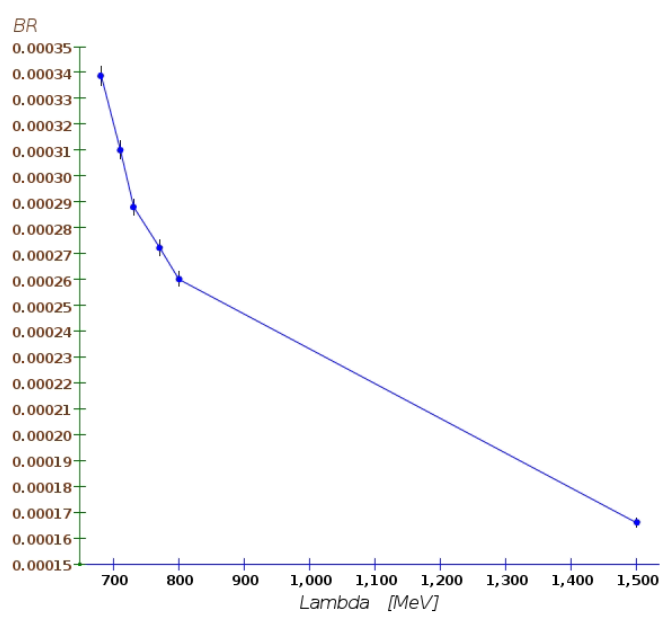
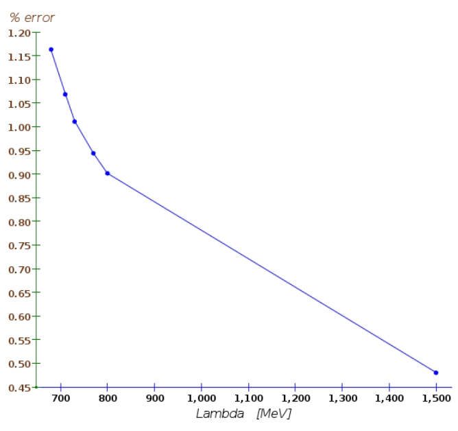
Figure 75: Branching ratio for the $\eta\rightarrow\gamma\mu^{+}\mu^{-}$ process (left) and statistical error on the $\varLambda$ parameter obtained with the branching ratio method (see text for details). The curves are for 3.3$\times$10¹⁵ POT

Line shape fitting method.

In this Approach, the uncertainty on the determination of the parameter $\varLambda$ is obtained from a fit of the invariant mass squared of the di-muon system: $s$=$\mid P_{\mu^{+}}+P_{\mu^{-}}\mid^{2}$. The fitting function is obtained by combining the amplitude in Eq. 128 with a three-body phase space distribution. The background contribution is described with a polynomial function, whose parameters are varied in the fit. The reconstruction efficiency is expected to be non-uniform over the rang of kinematically allowed values of s, especially near near threshold. This effect is taken into account by including a multiplicative polynomial function in the fit. The results of the fit for the event set corresponding to $\varLambda=800\,MeV$ is shown in the right plot of Fig. 75. We found that the determination of the parameter $\varLambda$ by the line shape fitting method is inferior to the branching ratio method, due to the weak dependence of the fitting function on $\varLambda$.

In conclusion, the statistical uncertainty estimated with the line shape fitting method is about one order of magnitude worse than the branching ratio method.

XIV.1.1 Concluding remark

We have examined REDTOP sensitivity to the determination of the $\varLambda$ parameter used to describe the form factor of the $\eta$ mesons. Two analyses where performed on a data sample corresponding $\sim$10^-5 of the total expected statistics. The statistical uncertainty on the measure of $\varLambda$ for a sample corresponding to 3.3$\times$10¹⁵ POT was found to be $\sim 1\%$ with the first method and one order of magnitude worse with the second method. This corresponds to an improvement of a factor $\sim 8\times$ compared to the measurement by the by A2 Coll. Aguar-Bartolome et al. (2014). When the statistics of the full event sample is taken into account, the projected statistical error on the measurement of the $\varLambda$ parameter is expected to be of the order of $10^{-4}$, presumably much smaller compared to the systematic error.

XV Discussion of the results

The studies presented in this manuscript suggest that, with a integrated luminosity of 3.3$\times 10^{18}$ POT, REDTOP has a very large potential for discovering New Physics by exploiting several rare processes. In particular, the branching ratio sensitivity for all decays of the $\eta$ meson where leptons are present in the final state, is in the range $\thickapprox 10^{-9}-10^{-8}$. This follows from how the experiment as been optimized, in particular for what the trigger system is concerned, having in mind a large rejection of the hadronic background in favor of the lighter and faster leptons. The performance of the detector, along with an unprecedented sample of $\eta$ mesons, allow REDTOP to probe all four portals connecting the Standard Model with the Dark Sector.

Since, we do not know a priory if a new particle. With a so called $"bump-hunt"$ analysis, the background is rejected with purely kinematics considerations. The level of rejection obtained with this simplified approach is already sufficient to reach a sensitivity for exploring uncharted regions of the parameter space in many theoretical models. That is also an indication the detector requirements for REDTOP have been chosen wisely (see, for example, the discussion in Sec. VI.3.

The second technique, the $\text{\textquotedblleft}detached-vertex\text{\textquotedblright}$ analysis, requires the presence of two reconstructed charged tracks with a common vertex, displaced from the primary vertex of the event. No Standard Model process is able of generating a similar event topology at the energies of interest for REDTOP. Consequently, the background rejection, is much more effective than for the $bump-hunt$ analysis, when long-lived particles are searched. For this technique to be successful, the target is split into thin foils, separated by enough distance to allow the long-lived particle, and its decay products, to leave undisturbed. A vertex detector with good position resolution is also an important ingredient. The sensitivity improvement obtained with the $\text{\textquotedblleft}detached\>vertex\text{\textquotedblright}$ analysis is very good, but it could be improved further with a more performing vertex detector. For this reason, the Fiber Tracker option will probably be dropped in favor of the Wafer-scale silicon sensor technology (cf. Sec. VI.4.1).

Besides the exploration of new particles and fields, the studies performed also indicate that REDTOP has a an excellent sensitivity to probe the conservation of discrete symmetries of the nature. This is achieved by studying the asymmetry in the distribution of certain observables related to the $\eta$ decays. We have demonstrated that, for nearly all processes considered in this work, the statistical uncertainty on those asymmetries will be much smaller than the typical systematic error. Therefore, it will be of paramount importance to have an excellent knowledge of the detector response, which is a key ingredient in reducing the systematic uncertainties. The very large event sample collected by REDTOP will help in that respect.

XVI Conclusions

The $\eta$ and $\eta^{\prime}$ mesons are almost unique in the particle universe. Carrying the same quantum number as the Higgs boson (except for parity), and no Standard Model charges, they represent an excellent laboratory for studying rare processes and new physics in the MeV–GeV energy range. The present world sample is too small to test violations of conservation laws or support searches for new particles that couple weakly to the Standard Model. A new $\eta/\eta$’-factory is being proposed: REDTOP. The goal is to produce $\mathcal{O}(10^{14})$ $\eta$ mesons and $\mathcal{O}(10^{12})$ $\eta^{\prime}$ in a few years of running. The sensitivity studies presented in this work indicate that, with such a large data sample and with a detector with REDTOP characteristics, the potential for discovering New Physics is very high for all four portals presently considered as links between dark matter and the Standard Model. Among existing and foreseen experiments, only SHiP at CERN has a similarly broad spectrum of research, although at a projected cost four times larger.

As discussed in detail in Sec. VIII, several outstanding anomalies could be investigated at REDTOP. The detector has excellent sensitivity for bosons decaying into $e^{+}e^{-}$ pairs with invariant masses below 17 MeV. Several theoretical models, across the Vector, Pseudoscalar, and Heavy Neutral Lepton portals, predict the existence such a particle. Full simulations has demonstrated the excellent sensitivity REDTOP to such models. One of those models Alves (2021), assumes that such a boson is, in fact, the long-searched Peccei-Quinn axion. We have demonstrated that REDTOP could discover such a particle, with sensitivity to a broad range of values of model parameters.

The anomalies observed by LSND and Miniboone could be explained by theoretical models with a new scalar particle and/or heavy neutral leptons. Two such models have been studied in this work: in both cases, the statistics and the performance of REDTOP appear to be sufficient for the discovery of such a particle. One of the models also explains the observed muon $g-2$ anomaly. In that context, we, also, presented sensitivity studies on the form-factors of the $\eta$ meson. The precision of that measurement is crucial for understanding $g-2$. Previous measurements on $\eta$ form-factors were based on samples $10^{7}$ smaller than that foreseen for REDTOP, using detectors with lower performance.

Many sensitivity studies presented in this work are related to the exploration of conservation laws in nature. $CP-$violation is one of the most important topics in particle physics, since it allows a model-independent search for new processes beyond the standard model. $CP$ symmetry can be explored at REDTOP in a multitude of different ways, thanks to large statistics and a well known background. In all cases, $CP$-violation is observed via asymmetries of observables related to the decays of the $\eta$ meson. An almost unique technique proposed in this work is based on the measurement of the polarization of the muon, copiously produced in several decays of the $\eta$. The muon is tagged by fully reconstructing its decay chain. This could be achieved either in the high-granularity, polarization-conserving, ADRIANO2 calorimeter or in a dedicated polarimeter. Furthermore, the proposed technique opens the road to a broader family of polarization measurements which will be discussed in a future work.

Recent LHCb results have highlighted the potential of Lepton Universality measurements to find new physics. REDTOP is well suited to explore the possible implications of those measurements in light-quark currents, if the underlying new physics is light. To this end, REDTOP exploits the abundant semileptonic decays of the $\eta$ meson and can, in principle, probe Lepton Universality with unprecedented precision. A dedicated discussion has been presented in this work, making the case for a sensitivity study based on a global analysis where light new physics is modeled in a general way.

This work also examined the related subject of the violation of lepton flavor in $\eta$ decays. REDTOP cannot, on this specific ground, compete with dedicated experiments based on muon beams. However the different mechanism of production of the muons might make this study interesting.

Although not discussed in this work, the composition of the $\eta$ and $\eta^{\prime}$ mesons has never been fully understood. Prior experiments indicate that only about 80% of the $\eta$ and $\eta^{\prime}$ constituents is represented by quark and gluons. The energy and momentum of the non-standard component indicate that this has, in fact, a non-zero mass. Unfortunately, as of this writing, there are no theoretical models capable of explaining such measurements. The discrepancy could be associated, in fact, to new particles or forces. REDTOP will try to address those aspects of $\eta$ physics in future studies.

An important aspect of REDTOP is related to the detector technologies chosen for the experiment. With an event rate of 700 kHz, a factor almost 18 times larger than LHCb, REDTOP is the, collider-style experiment, with the fastest Level-0 trigger ever considered. In spite of the relatively low momentum of the charged tracks to be detected, a realm once restricted to low-mass gaseous detectors, such an event rate requires that the tracking system be based on solid state technologies. Still, the material budgets needs to be appreciably smaller and more radiation resistant than existing detectors. On the other side, the, recently approved, EIC project has very similar requirements for its tracking systems, and the detector technologies explored are similar to those proposed for REDTOP. Synergies and common activities between the two programs are being discussed as of this writing.

New Physics is being searched for at REDTOP predominantly in association with leptons. In a hadron-produced environment, particle identification is, therefore of crucial importance. A relatively novel dual-readout technique, has been identified to push lepton-hadron separation to a new level. The ADRIANO2 technology, currently under development, adds time-of-flight capabilities to dual-readout, for a full 5-D reconstruction of the showers. The ongoing R&D on all such techniques, while crucial for the success of REDTOP, will benefit several future experiments in high energy and nuclear science.

There is no doubt that REDTOP is a challenging experiment, requiring at the same time, rapid response, high precision and radiation hardness. On the other hand, the requirements on the accelerator are very tame, requiring only 30-60 W of proton beam. Several laboratories have expressed interest in hosting the experiment.

Due to its relatively small size, the projected cost of the detector is only $M50-80. The low cost required to adapt an existing accelerator and the availability of unused superconducting solenoid help to control the cost. The physics case for a super-$\eta$/$\eta^{\prime}$ factory is very strong and well supported by the theoretical community. The cost is well justified by REDTOP’s broad scope for exploration of new physics, making this experiment very attractive.

When future low-energy, MegaWatt class accelerator facilities will become available (PIPII, ESS, CSNS), REDTOP could be eventually upgraded to a tagged $\eta$-factory experiment, with a similar $\eta$-meson yield but with the obvious advantage of $\eta$-tagging. Therefore REDTOP should be considered more like an exploration facility than a single experiment, offering the opportunity of a precise observatory on New Physics and a multi-year research program.

XVII Appendix I: The Acceleration Scheme

Although the beam requirements for REDTOP are modest, none of the existing HEP laboratories worldwide as a ready-to-go accelerator satisfying all the conditions. The Collaboration has engaged in a broad exploration and several possible hosting laboratories have been identified.

XVII.1 Fermilab configuration.

The low energy proton beam available at Fermilab has a pulsed structure with 84 bunches and a fixed energy of 8 GeV. The buckets are distributed to the accelerator complex and either accelerated or dumped in order to create a secondary beam. On the other hand, REDTOP requires a Continuous Wave (CW) proton beam with a user selectable energy, with a range considerably lower than that available (cf. Sec. VI). The accelerator scheme(Syphers and Johnstone, 2016) proposed for REDTOP foresee the extraction of a single pulse from the booster (consisting of $\sim$4$\times$10¹² protons) which is subsequently injected in the Delivery Ring (former debuncher in anti-proton production at Tevatron). The energy is, then removed from the beam by operating the RF cavities in reverse, until it reaches the required value. The time required for reaching 1.8 Gev is $\sim$5 seconds (about 3.3 for the 3.5 GeV case). Once the desired energy is reached, the beam is kept circulating inside the ring where the buckets relax adiabatically. Slow extraction to REDTOP (located in the nearby AP50 hall) occur over $\sim$40 seconds. The proposed accelerator scheme requires minimal changes to the existing complex and involves no extra beam elements. In fact, the extra RF cavity necessary to stabilize the energy removal process is already available as a spare for the Mu2e experiment. Furthermore, the extraction point to AP50 corresponds to a betatron phase advance of 270^o compared to the location of the existing Mu2e electrostatic septum. Consequently, the latter can be used also to shift the protons for the final extraction via a Lambertson magnet. The total time to decelerate-debunch-extract the beam is 51 sec, corresponding to a duty cycle $\sim$80%.

With the above scheme, large beam losses in the Delivery Ring will occur if beam is decelerated from injection at 8 GeV (corresponding to $\gamma$=9.53) to <2 GeV ($\gamma$ = 3.13) through the natural transition energy of the ring: $\gamma{}_{t}$ = 7.64. Transition can, however, be avoided by using select quadrupole triplets to boost $\gamma{}_{t}$ above beam $\gamma$ by 0.5 units throughout deceleration until $\gamma{}_{t}$ = 7.64 and beam $\gamma$ = 7.14 (corresponding to E_kin=5.76 GeV ). Below 5.76 GeV the Delivery Ring lattice is reverted to the nominal design configuration. Optical perturbations are localized within each triplet while the straight sections are unaffected thereby keeping the nominal M3 injection beamline tune valid(Syphers and Johnstone, 2016).

Achieving the full set of goals of the experiment will require production and processing of at least $10^{13}$ $\eta$ meson decays. The goals can be met by having a flux of $10^{11}$ protons per second on target, and a duty factor of over 75%. The Fermilab Booster routinely delivers $4\times 10^{12}$ protons per cycle at up to 15-Hz repetition rate. Thus, there should be an abundance of protons to meet the REDTOP goals. However, the Booster extraction kinetic energy is 8 GeV, well above the $\sim$2 GeV and 3 GeV needed for REDTOP to produce, respectively, $\eta$ and $\eta^{\prime}$ mesons. A deceleration stage will be implemented.

XVII.2 CERN configuration.

A preliminary study has been performed at CERN to provide a beam with REDTOP’s requirements. Several possible schemes have been considered, the most promising corresponding to the extraction of a 1.8 GeV beam from the ProtoSynchrotron (PS) which could then be delivered to the East Hall, where the experiment could be housed. For the moment a 24 GeV/c proton beam is routinely slow-extracted into the CHARM and IRRAD facilities along the T8 beam line with a maximum intensity of 6.5$\times$10¹¹ protons per extraction over 0.4 seconds. REDTOP would require a much longer flat top of e.g. 10 seconds at $\sim$1.8 GeV kinetic energy (as it can be delivered directly from the PS Booster) in a cycle of 9 basic periods(10.8 s). No show-stoppers have been identified up to date, although more studies are required. However, the PS the duty cycle cannot be much higher than 50%, which would already have a significant impact on the existing CERN physics program. Consequently, the expected luminosity available to REDTOP at CERN is expected to be $\sim\nicefrac{{1}}{{10}}$ of that available at Fermilab.

XVII.3 BNL configuration.

AT BNL the REDTOP detector could sit comfortably at the end of the existing C4 extraction line. Logistics would be optimal, since the experimental hall is well accessible and serviced. The beam would be slowly extracted from the AGS using well known techniques. The instrumentation electronics of the extraction line is no longer functional and it needs to be refurbished at a very modest cost estimated of order ($\mathcal{O}$(100K$)). Altogether, BNL is an excellent candidate for hosting REDTOP.

XVII.4 HIAF configuration.

The REDTOP detector can be installed at the Multi-function terminal of the HIAF accelerator. The beam extracted from the Booster Ring ($BRing$) fullfil all requirements for REDTOP experiment (cf. Sec. VI.2). The transfer beam line construction is already included in the HIAF project. The maximum magnetic rigidity is 34 Tm, corresponding to a maximum proton beam energy of 9.3 GeV. The facility is expected to be operational around 2025 for a run above the $\eta^{\prime}$ production threshold with a beam density equal or exceeding 1$\times$10¹³ protons-per-spill.

XVII.5 GSI configuration.

As a possible alternative, the use of the SIS18 beam at GSI/FAIR could be considered, since the necessary energies and intensities could be provided by the existing accelerators. An assessment of the feasibility of the experiment in this laboratory will be started after the submission of this White Paper.

XVIII Appendix II: Tagged $\eta$-factory

An upgraded version of the REDTOP, t-REDTOP Arrington et al. (2022), could be run in a later stage of the experiment at the PIP-II facility, currently under construction at Fermilab. At the 800 MeV, high intensity (100KW-1MW), CW proton beam, the production mechanism of the $\eta$-meson is substantially different. The nuclear process providing the $\eta$-meson would be:

$$p+De\rightarrow\eta+^{3}He^{+}$$ (130)

Therefore, t-REDTOP requires a gaseous Deuterium target and an extra detector to tag the ${}^{3}He^{+}$ ion. The production cross section for the process (130) is approximately five orders of magnitude smaller than at 1.8 GeV and the gaseous target reduces further the luminosity of the beam. However, the large intensity of PIP-II more than compensate for that and the number of $\eta-mesons$ produced at t-REDTOP is expected to be in the range [$10^{13}/year-10^{14}/year$]. The biggest advantages of a tagged $\eta$-factory are the following:

• By tagging the production of the $\eta$-meson via the detection of the ${}^{3}He^{+}$ ion, the combinatorics background from $non-\eta$ events, is greatly diminished. Consequently, the sensitivity of the experiment to New Physics is increased by a factor proportional to the square root of that reduction;

• By measuring the momentum of the ${}^{3}He^{+}$ ion in process (130), the kinematics of the reaction is fully closed. That portends to a better measurements of the kinematics of the particles detected, since a 4-C kinematic fit could be applied;

• Since the kinematics is closed, any long lived, dark particle escaping detection could be identified using the missing 4-momentum technique. The latter is considerably more powerful than the, 1-, missing p_t or missing energy proposed by some recent experiments searching for dark matter.

The disadvantages of a tagged-$\eta$ experiment are due mostly to the larger complexity of the experiment, requiring an extra detector at very small angles and to the necessity to control the halo of the beam at a much higher level. Also, the mass of New Physics explored will be lower, since no $\eta^{\prime}$-meson could be produced at the PIP-II design energy.

XIX Appendix III: Radiation Damage and Detector Aging

The intense proton beam required for reaching REDTOP’s physics goal is also expected to generate a radiation halo that will age and could potentially damage the detector. Descriptions of the detector components are contained in Sec. VI.4.

An analysis of the radiation flux expected throughout the detector has been performed with the MARS15 code Mokhov (2016) and a geometrical model that reflects our baseline detector layout, along with an aluminum-Borated Polyethylene-barite beam dump. The result of a study for a 30-W proton beam with 1.8-GeV energy impinging onto the beryllium target systems is shown in Fig. 76. The plot represents the so-called “1-MeV equivalent neutron fluence” (NEQF) dose, which is commonly used to estimate the damage inflicted by radiation to photo-sensors.

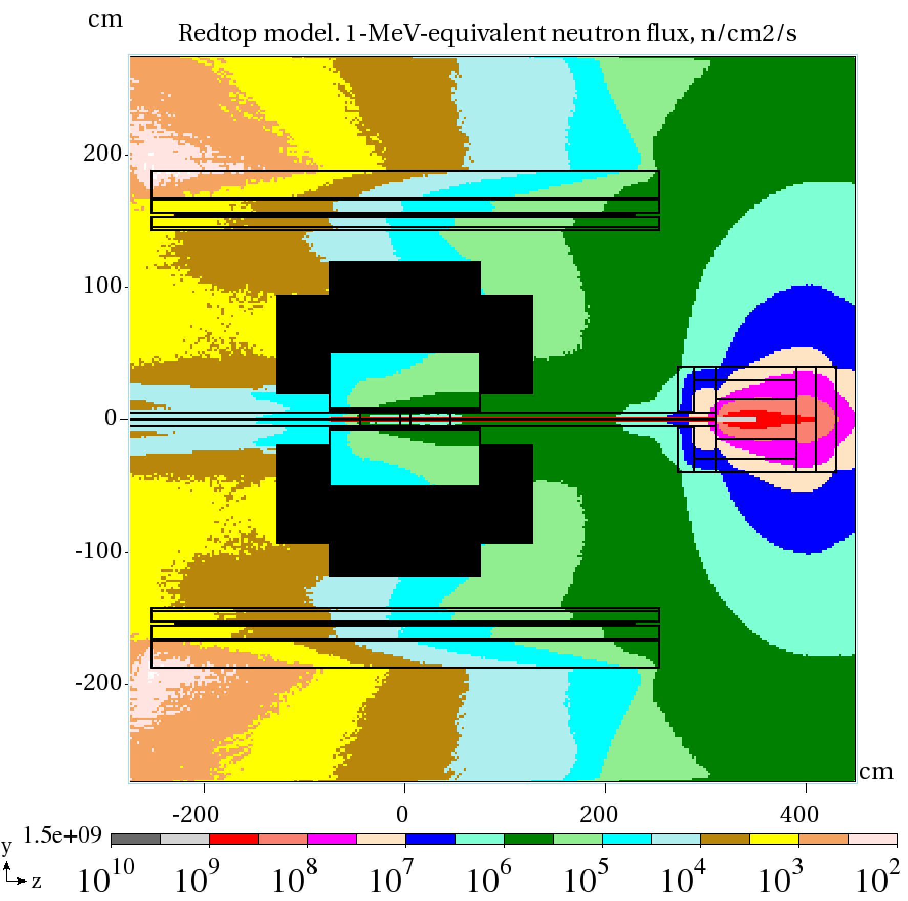
Figure 76: “1-MeV equivalent neutron fluence” dose expected in the REDTOP detector for a 30-W proton beam.

The areas of concern are the photo-sensors around the vessel of the OTPC and the area around the beam pipe that is planned to be instrumented with a scintillating fiber tracker (cf. Sec. VI.4). The maximum NEQF flux illuminating the photo-sensors is located on the forward endplate of the of OTPC and is expected to be about $6\times 10^{5}$/cm²/s (or $6\times 10^{12}$/cm² integrated over 1 year). The rate for the barrel is, in average, a factor of 5-6 lower. The currently recognized integrated limit for commercial SiPMs, the current baseline technology adopted for the OTPC, corresponds to about 10¹³/cm² NEQF. The value is uncomfortably close to the estimated flux in the end plates. A consequence is an increase in the dark count rate (DCR) of the sensors (typically, 50 kHz/mm² or 250 OTPC hits/evt for a 1-ns integration time). While the effect of such noise is expected to be minimal on the reconstruction of C̆erenkov rings, a bigger issue would come from the saturation of the online systems which could compromise the data transfer of the compressed data from the detector to the L0 trigger systems. We are aware of the issue and plan to investigate it further. Possible roads we will consider to mitigate an increased DCR are:

• A larger bandwidth between the FEE and the L0 trigger systems;

• Cooling the SiPM’s;

• Narrowing the integration time;

• Investigate new generation sensors (e.g. addition of trenches between pixels to reduce cross talk);

• Using Multichannel plates for the forward endplate and SiPMs for the remainder of the detector;

• Consider LAPPD instead of Sipm’s, although the formers are not yet commercially available.

In addition to these items, the LHC Community is very active in this area and we expect to benefit greatly from the R&D performed by them.

The area near the beam pipe, where the fiber tracker will be located, is currently under study. Recent studies by LHCb Joram et al. (2015) where fibers have been tested up to 60 kGy, is summarized in Fig. 77, where the change in attenuation length is plotted vs. the radiation dose. In the case of REDTOP, we expect that the fiber tracker would degrade considerably during a 1-year run, with the attenuation length of a typical KURARAY SCSF-78 fiber (⌀250 $\mu$m), diminishing from about 4 m to 10  cm. We are aware of the issues and plan to investigate them further.

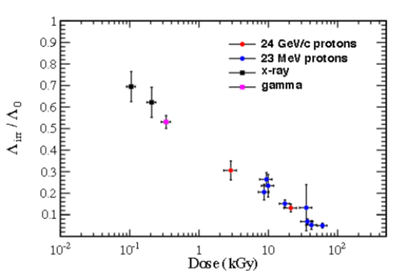
Figure 77: Change in attenuation length of a KURARAY SCSF-78 fiber (⌀250 $\mu$m) vs. integrated dose.

XX Appendix IV: Radiation Shielding and Safety

The experimental hall proposed for REDTOP, AP50, is part of Fermilab’s “Muon Campus” where two experiments are or will be running (Muon g-2 and Mu2e). All areas related to the Muon Campus are under close scrutiny by the Fermilab Safety Dept., and a full radiation shielding assessment has been recently completed and approved by the ESHQ Office. According to the latter, a maximum beam intensity of $3.60\times 10^{13}$ protons/hr at 8 GeV can be circulated and delivered in the accelerator complex where AP50 is located, with the current radiation shielding, while 2.20x10¹⁶ protons/hr can be circulated with the modification foreseen for Mu2e. The latter rate corresponds to a maximum beam power circulated and dumped of 8 kW, to be compared with the 30 W proposed to run REDTOP as an $\eta$-factory, and the 50 W proposed for a later run as an $\eta^{\prime}$-factory. In both cases, the proposed beam intensity is considerably smaller than the maximum allowed and it requires no refurbishing of the existing radiation shielding.

References

- Batell et al. (2009a) B. Batell, M. Pospelov, and A. Ritz, Phys. Rev. D 80, 095024 (2009a), URL https://link.aps.org/doi/10.1103/PhysRevD.80.095024.
- Reece and Wang (2009) M. Reece and L.-T. Wang, Journal of High Energy Physics 2009, 051 (2009), ISSN 1029-8479, URL http://dx.doi.org/10.1088/1126-6708/2009/07/051.
- Bjorken et al. (2009) J. D. Bjorken, R. Essig, P. Schuster, and N. Toro, Physical Review D 80 (2009), ISSN 1550-2368, URL http://dx.doi.org/10.1103/PhysRevD.80.075018.
- Batell et al. (2009b) B. Batell, M. Pospelov, and A. Ritz, Phys. Rev. D 80, 095024 (2009b), URL https://link.aps.org/doi/10.1103/PhysRevD.80.095024.
- Frisch (2014) H. Frisch, Technical scope of work for o-tpc. (2014), URL https://web.fnal.gov/experiment/FTBF/TSW%20Library/T1059_tsw.pdf.
- et al. (2020) P. J. V. et al., Eur. Phys. J. A 56, 183 (2020).
- M.Thomson (2006) M.Thomson (2006), https://arxiv.org/abs/physics/0607261v1.
- Krnjaic (2020) G. Krnjaic, Dark matter production at high intensities (2020), URL https://indico.fnal.gov/event/44819/contributions/193751/attachments/132857/163535/RF6-Kickoff-DM-Production.pdf.
- Nefkens (1996) B. Nefkens (1996), https://www.phy.bnl.gov/ags-2000/eta/eta.html, URL https://www.phy.bnl.gov/ags-2000/eta/eta.html.
- Singh and Patel (2011) J. P. Singh and A. B. Patel, Journal of Physics G: Nuclear and Particle Physics 39, 015006 (2011), URL https://doi.org/10.1088/0954-3899/39/1/015006.
- Gunion et al. (2000) J. F. Gunion, H. E. Haber, G. L. Kane, and S. Dawson, The Higgs Hunter’s Guide, vol. 80 (Westview Press, 2000).
- Bae et al. (2012) K. J. Bae, K. Choi, E. J. Chun, S. H. Im, C. B. Park, and C. S. Shin, Journal of High Energy Physics 2012 (2012), ISSN 1029-8479, URL http://dx.doi.org/10.1007/JHEP11(2012)118.
- Peccei and Quinn (1977a) R. D. Peccei and H. R. Quinn, Phys. Rev. D 16, 1791 (1977a), URL https://link.aps.org/doi/10.1103/PhysRevD.16.1791.
- Weinberg (1978a) S. Weinberg, Phys. Rev. Lett. 40, 223 (1978a), URL https://link.aps.org/doi/10.1103/PhysRevLett.40.223.
- Langacker (2009) P. Langacker, Reviews of Modern Physics 81, 1199 (2009), ISSN 1539-0756, URL http://dx.doi.org/10.1103/RevModPhys.81.1199.
- Holdom (1986) B. Holdom, Physics Letters B 166, 196 (1986), ISSN 0370-2693, URL https://www.sciencedirect.com/science/article/pii/0370269386913778.
- et al. (2016) C. P. et al., Chinese Physics C 40, 100001 (2016), URL https://doi.org/10.1088/1674-1137/40/10/100001.
- Adrian et al. (2018) P. H. Adrian, N. A. Baltzell, M. Battaglieri, M. Bondí, S. Boyarinov, S. Bueltmann, V. D. Burkert, D. Calvo, M. Carpinelli, A. Celentano, et al. (Heavy Photon Search Collaboration), Phys. Rev. D 98, 091101 (2018), URL https://link.aps.org/doi/10.1103/PhysRevD.98.091101.
- Raggi et al. (2015) M. Raggi, V. Kozhuharov, and P. Valente, The padme experiment at lnf (2015), eprint 1501.01867.
- et al. (2019) J. B. et al., Journal of Physics G: Nuclear and Particle Physics 47, 010501 (2019), URL https://doi.org/10.1088/1361-6471/ab4cd2.
- Tulin (2014) S. Tulin, Phys. Rev. D 89, 114008 (2014), eprint 1404.4370.
- Escribano et al. (2020) R. Escribano, S. Gonzàlez-Solís, R. Jora, and E. Royo, Phys. Rev. D 102, 034026 (2020), eprint 1812.08454.
- Bramon et al. (1992) A. Bramon, A. Grau, and G. Pancheri, Phys. Lett. B 283, 416 (1992).
- Kubis and Plenter (2015) B. Kubis and J. Plenter, Eur. Phys. J. C 75, 283 (2015), eprint 1504.02588.
- Stollenwerk et al. (2012) F. Stollenwerk, C. Hanhart, A. Kupść, U.-G. Meißner, and A. Wirzba, Phys. Lett. B 707, 184 (2012), eprint 1108.2419.
- Feng et al. (2016) J. L. Feng, B. Fornal, I. Galon, S. Gardner, J. Smolinsky, T. M. P. Tait, and P. Tanedo, Phys. Rev. Lett. 117, 071803 (2016), URL https://link.aps.org/doi/10.1103/PhysRevLett.117.071803.
- Feng et al. (2017) J. L. Feng, B. Fornal, I. Galon, S. Gardner, J. Smolinsky, T. M. P. Tait, and P. Tanedo, Phys. Rev. D 95, 035017 (2017), eprint 1608.03591.
- Krasznahorkay et al. (2016) A. J. Krasznahorkay et al., Phys. Rev. Lett. 116, 042501 (2016), eprint 1504.01527.
- Miller et al. (2007) J. P. Miller, E. de Rafael, and B. Lee Roberts, Reports on Progress in Physics 70, R03 (2007), ISSN 1361-6633, URL http://dx.doi.org/10.1088/0034-4885/70/5/R03.
- Banerjee et al. (2020) D. Banerjee et al. (NA64), Phys. Rev. D 101, 071101 (2020), eprint 1912.11389.
- Depero et al. (2020) E. Depero et al. (NA64), Eur. Phys. J. C 80, 1159 (2020), eprint 2009.02756.
- Krasznahorkay et al. (2021) A. J. Krasznahorkay, M. Csatlós, L. Csige, J. Gulyás, A. Krasznahorkay, B. M. Nyakó, I. Rajta, J. Timár, I. Vajda, and N. J. Sas, Phys. Rev. C 104, 044003 (2021), eprint 2104.10075.
- Feng et al. (2020) J. L. Feng, T. M. P. Tait, and C. B. Verhaaren, Phys. Rev. D 102, 036016 (2020), eprint 2006.01151.
- Zhang and Miller (2021) X. Zhang and G. A. Miller, Phys. Lett. B 813, 136061 (2021), eprint 2008.11288.
- Adler (1969) S. L. Adler, Phys. Rev. 177, 2426 (1969).
- Bell and Jackiw (1969) J. S. Bell and R. Jackiw, Nuovo Cim. A 60, 47 (1969).
- Fujiwara et al. (1985) T. Fujiwara, T. Kugo, H. Terao, S. Uehara, and K. Yamawaki, Prog. Theor. Phys. 73, 926 (1985).
- Ng and Peters (1992) J. N. Ng and D. J. Peters, Phys. Rev. D 46, 5034 (1992), URL https://link.aps.org/doi/10.1103/PhysRevD.46.5034.
- Ng and Peters (1993) J. N. Ng and D. J. Peters, Phys. Rev. D 47, 4939 (1993), URL https://link.aps.org/doi/10.1103/PhysRevD.47.4939.
- Shabalin (2002) E. Shabalin, Physica Scripta T99, 104 (2002), URL https://doi.org/10.1238/physica.topical.099a00104.
- Escribano and Royo (2020) R. Escribano and E. Royo, Eur. Phys. J. C 80, 1190 (2020), [Erratum: Eur.Phys.J.C 81, 140 (2021)], eprint 2007.12467.
- D’Ambrosio et al. (2002) G. D’Ambrosio, G. F. Giudice, G. Isidori, and A. Strumia, Nucl. Phys. B 645, 155 (2002), eprint hep-ph/0207036.
- Egana-Ugrinovic et al. (2019a) D. Egana-Ugrinovic, S. Homiller, and P. Meade, Phys. Rev. Lett. 123, 031802 (2019a), URL https://link.aps.org/doi/10.1103/PhysRevLett.123.031802.
- Egana-Ugrinovic et al. (2020) D. Egana-Ugrinovic, S. Homiller, and P. Meade, Phys. Rev. Lett. 124, 191801 (2020), URL https://link.aps.org/doi/10.1103/PhysRevLett.124.191801.
- Batell et al. (2019) B. Batell, A. Freitas, A. Ismail, and D. Mckeen, Phys. Rev. D 100, 095020 (2019), eprint 1812.05103.
- Egana-Ugrinovic et al. (2019b) D. Egana-Ugrinovic, S. Homiller, and P. R. Meade, Phys. Rev. D 100, 115041 (2019b), eprint 1908.11376.
- Egana-Ugrinovic et al. (2021) D. Egana-Ugrinovic, S. Homiller, and P. Meade, Phys. Rev. D 103, 115005 (2021), eprint 2101.04119.
- Batell et al. (2018) B. Batell, A. Freitas, A. Ismail, and D. Mckeen, Phys. Rev. D 98, 055026 (2018), eprint 1712.10022.
- Batell et al. (2021) B. Batell, A. Freitas, A. Ismail, D. McKeen, and M. Rai, Phys. Rev. D 104, 115032 (2021), eprint 2107.08059.
- Kling and Trojanowski (2021) F. Kling and S. Trojanowski, Phys. Rev. D 104, 035012 (2021), eprint 2105.07077.
- Abdallah et al. (2021) W. Abdallah, R. Gandhi, and S. Roy, Phys. Rev. D 104, 055028 (2021), eprint 2010.06159.
- O’Connell et al. (2007a) D. O’Connell, M. J. Ramsey-Musolf, and M. B. Wise, Phys. Rev. D 75, 037701 (2007a), URL https://link.aps.org/doi/10.1103/PhysRevD.75.037701.
- Krnjaic (2016) G. Krnjaic, Phys. Rev. D 94, 073009 (2016), URL https://link.aps.org/doi/10.1103/PhysRevD.94.073009.
- Alemany et al. (2019) R. Alemany et al. (2019), to be published in Journal of Physics G: Nuclear and Particle Physics, eprint 1902.00260.
- Gan et al. (2022) L. Gan, B. Kubis, E. Passemar, and S. Tulin, Phys. Rept. 945, 2191 (2022), eprint 2007.00664.
- Peccei and Quinn (1977b) R. D. Peccei and H. R. Quinn, Phys. Rev. Lett. 38, 1440 (1977b).
- Peccei and Quinn (1977c) R. D. Peccei and H. R. Quinn, Phys. Rev. D 16, 1791 (1977c), URL https://link.aps.org/doi/10.1103/PhysRevD.16.1791.
- Weinberg (1978b) S. Weinberg, Phys. Rev. Lett. 40, 223 (1978b), URL https://link.aps.org/doi/10.1103/PhysRevLett.40.223.
- Wilczek (1978) F. Wilczek, Phys. Rev. Lett. 40, 279 (1978), URL https://link.aps.org/doi/10.1103/PhysRevLett.40.279.
- Bardeen et al. (1987) W. A. Bardeen, R. D. Peccei, and T. Yanagida, Nucl. Phys. B279, 401 (1987).
- Alves and Weiner (2018) D. S. M. Alves and N. Weiner, JHEP 07, 092 (2018), eprint 1710.03764.
- Andreev et al. (2021) Y. M. Andreev et al. (NA64), Phys. Rev. D 104, L111102 (2021), eprint 2104.13342.
- Alves (2021) D. S. Alves, Phys. Rev. D 103, 055018 (2021).
- Krasznahorkay et al. (2019) A. J. Krasznahorkay et al. (2019), eprint 1910.10459.
- Abouzaid et al. (2007) E. Abouzaid et al. (KTeV), Phys. Rev. D75, 012004 (2007), eprint hep-ex/0610072.
- Ecker et al. (1989) G. Ecker, J. Gasser, A. Pich, and E. de Rafael, Nucl. Phys. B321, 311 (1989).
- Bargholtz et al. (2007) C. Bargholtz, M. Bashkanov, D. Bogoslawsky, H. Calén, F. Cappellaro, H. Clement, L. Demirörs, C. Ekström, K. Fransson, L. Gerén, et al., Physics Letters B 644, 299 (2007), ISSN 0370-2693, URL https://www.sciencedirect.com/science/article/pii/S0370269306015280.
- Ablikim et al. (2013) M. Ablikim, M. N. Achasov, O. Albayrak, D. J. Ambrose, F. F. An, Q. An, J. Z. Bai, R. Baldini Ferroli, Y. Ban, J. Becker, et al. (BESIII Collaboration), Phys. Rev. D 87, 092011 (2013), URL https://link.aps.org/doi/10.1103/PhysRevD.87.092011.
- Bauer et al. (2021) M. Bauer, M. Neubert, S. Renner, M. Schnubel, and A. Thamm, Phys. Rev. Lett. 127, 081803 (2021), eprint 2102.13112.
- Alves and Gonzàlez-Solís (2022) D. S. M. Alves and S. Gonzàlez-Solís, To appear (2022).
- Escribano and Frere (2005) R. Escribano and J.-M. Frere, JHEP 06, 029 (2005), eprint hep-ph/0501072.
- Nef (1994) Proceedings of the International Conference on Mesons and Nuclei at Intermediate Energie (1994).
- Prakhov et al. (2000) S. Prakhov, W. B. Tippens, C. Allgower, V. Bekrenev, E. Berger, W. J. Briscoe, M. Clajus, J. R. Comfort, K. Craig, D. Grosnick, et al. (Crystal Ball Collaboration), Phys. Rev. Lett. 84, 4802 (2000), URL https://link.aps.org/doi/10.1103/PhysRevLett.84.4802.
- collaboration et al. (2008) T. K. collaboration, F. Ambrosino, A. Antonelli, M. Antonelli, F. Archilli, C. Bacci, P. Beltrame, G. Bencivenni, S. Bertolucci, C. Bini, et al., Journal of High Energy Physics 2008, 006 (2008), URL https://doi.org/10.1088/1126-6708/2008/05/006.
- Lee and Wolfenstein (1965) T. D. Lee and L. Wolfenstein, Phys. Rev. 138, B1490 (1965).
- Nauenberg (1965) M. Nauenberg, Phys. Lett. 17, 329 (1965).
- Lee (1965) T. D. Lee, Phys. Rev. 139, B1415 (1965).
- Gardner and Shi (2020) S. Gardner and J. Shi, Phys. Rev. D 101, 115038 (2020), URL https://link.aps.org/doi/10.1103/PhysRevD.101.115038.
- Grzadkowski et al. (2010) B. Grzadkowski, M. Iskrzynski, M. Misiak, and J. Rosiek, JHEP 10, 085 (2010), eprint 1008.4884.
- Shi (2020) J. Shi, Ph.D. thesis, Kentucky U. (2020).
- Gardner and Shi (2022) S. Gardner and J. Shi (2022), in preparation.
- Gardner and Tandean (2004) S. Gardner and J. Tandean, Phys. Rev. D 69, 034011 (2004), URL https://link.aps.org/doi/10.1103/PhysRevD.69.034011.
- Burgess et al. (2021) C. P. Burgess, S. Hamoudou, J. Kumar, and D. London (2021), eprint 2111.07421.
- Akdag et al. (2022) H. Akdag, T. Isken, and B. Kubis, JHEP 02, 137 (2022), eprint 2111.02417.
- Layter et al. (1972) J. G. Layter, J. A. Appel, A. Kotlewski, W. Lee, S. Stein, and J. J. Thaler, Phys. Rev. Lett. 29, 316 (1972), URL https://link.aps.org/doi/10.1103/PhysRevLett.29.316.
- Anastasi et al. (2016) A. Anastasi et al. (KLOE-2), JHEP 05, 019 (2016), eprint 1601.06985.
- Gasser and Leutwyler (1985) J. Gasser and H. Leutwyler, Nucl. Phys. B 250, 539 (1985).
- Anisovich and Leutwyler (1996) A. V. Anisovich and H. Leutwyler, Phys. Lett. B 375, 335 (1996), eprint hep-ph/9601237.
- Lanz (2011) S. Lanz, Ph.D. thesis, Bern U. (2011), eprint 1809.10110.
- Bijnens and Ghorbani (2007) J. Bijnens and K. Ghorbani, JHEP 11, 030 (2007), eprint 0709.0230.
- Watson (1954) K. M. Watson, Phys. Rev. 95, 228 (1954).
- Gardner et al. (2001) S. Gardner, U.-G. Meißner, and G. Valencia, Phys. Lett. B 508, 44 (2001), eprint hep-ph/0103144.
- Barrett et al. (1966) B. Barrett, M. Jacob, M. Nauenberg, and T. N. Truong, Phys. Rev. 141, 1342 (1966).
- Herczeg and Singer (1973) P. Herczeg and P. Singer, Phys. Rev. D 8, 4107 (1973), URL https://link.aps.org/doi/10.1103/PhysRevD.8.4107.
- Geng et al. (2002) C. Q. Geng, J. N. Ng, and T. H. Wu, Modern Physics Letters A 17, 1489 (2002), ISSN 1793-6632, URL http://dx.doi.org/10.1142/S0217732302007697.
- Gao (2002) D.-N. Gao, Modern Physics Letters A 17, 1583 (2002).
- Ambrosino et al. (2009) F. Ambrosino, A. Antonelli, M. Antonelli, F. Archilli, P. Beltrame, G. Bencivenni, S. Bertolucci, C. Bini, C. Bloise, S. Bocchetta, et al., Physics Letters B 675, 283 (2009).
- Adlarson et al. (2016) P. Adlarson, W. Augustyniak, W. Bardan, M. Bashkanov, F. S. Bergmann, M. Berłowski, H. Bhatt, A. Bondar, M. Büscher, H. Calén, et al. (WASA-at-COSY Collaboration), Phys. Rev. C 94, 065206 (2016), URL https://link.aps.org/doi/10.1103/PhysRevC.94.065206.
- Ablikim et al. (2021) M. Ablikim, M. N. Achasov, P. Adlarson, S. Ahmed, M. Albrecht, A. Amoroso, Q. An, X. H. Bai, Y. Bai, O. Bakina, et al. (BESIII Collaboration), Phys. Rev. D 103, 092005 (2021), URL https://link.aps.org/doi/10.1103/PhysRevD.103.092005.
- Adlarson et al. (2015) P. Adlarson et al. (2015), arXiv:1509.06588.
- Sanchez-Puertas (2019) P. Sanchez-Puertas, JHEP 01, 031 (2019), eprint 1810.13228.
- Masjuan and Sanchez-Puertas (2016) P. Masjuan and P. Sanchez-Puertas, JHEP 08, 108 (2016), eprint 1512.09292.
- Yanase et al. (2019) K. Yanase, N. Yoshinaga, K. Higashiyama, and N. Yamanaka, Phys. Rev. D 99, 075021 (2019), eprint 1805.00419.
- Sanchez-Puertas (2021) P. Sanchez-Puertas, Nucl. Part. Phys. Proc. 312-317, 15310 (2021), eprint 1909.07491.
- Abel et al. (2020) C. Abel et al., Phys. Rev. Lett. 124, 081803 (2020), eprint 2001.11966.
- Escribano et al. (2022a) R. Escribano, E. Royo, and P. Sanchez-Puertas (2022a), eprint 2202.04886.
- Hazard and Petrov (2018) D. Hazard and A. A. Petrov, Physical Review D 98 (2018), ISSN 2470-0029, URL http://dx.doi.org/10.1103/PhysRevD.98.015027.
- Hazard and Petrov (2016a) D. E. Hazard and A. A. Petrov, Physical Review D 94 (2016a), ISSN 2470-0029, URL http://dx.doi.org/10.1103/PhysRevD.94.074023.
- (109) S.D. Drell, Direct decay , Nuovo Cim. 11, 693-697 (1959).
- Berman and Geffen (1960) S. Berman and D. Geffen, Nuovo Cim. 18, 1192 (1960).
- Geffen and Young (1965) D. A. Geffen and B.-l. Young, Phys. Rev. Lett. 15, 316 (1965).
- Abegg et al. (1994) R. Abegg et al., Phys. Rev. D 50, 92 (1994).
- Landsberg (1985) L. G. Landsberg, Phys. Rept. 128, 301 (1985).
- Mayer (1990) B. Mayer, ed., Rare decays of light mesons. Proceedings, International Workshop, Gif-sur-Yvette, France, March 29-30, 1990 (1990), D. Wyler (p. 125).
- Hazard and Petrov (2016b) D. E. Hazard and A. A. Petrov, Phys. Rev. D 94, 074023 (2016b), eprint 1607.00815.
- Glashow et al. (2015) S. L. Glashow, D. Guadagnoli, and K. Lane, Phys. Rev. Lett. 114, 091801 (2015), eprint 1411.0565.
- Guadagnoli and Lane (2015) D. Guadagnoli and K. Lane, Phys. Lett. B 751, 54 (2015), eprint 1507.01412.
- Borsato et al. (2019) M. Borsato, V. V. Gligorov, D. Guadagnoli, D. Martinez Santos, and O. Sumensari, Phys. Rev. D 99, 055017 (2019), eprint 1808.02006.
- Albaladejo et al. (2021) M. Albaladejo et al. (JPAC) (2021), eprint 2112.13436.
- Bell and Sutherland (1968) J. S. Bell and D. G. Sutherland, Nucl. Phys. B 4, 315 (1968).
- Sutherland (1966) D. G. Sutherland, Phys. Lett. 23, 384 (1966).
- Baur et al. (1996) R. Baur, J. Kambor, and D. Wyler, Nucl. Phys. B 460, 127 (1996), eprint hep-ph/9510396.
- Ditsche et al. (2009) C. Ditsche, B. Kubis, and U.-G. Meißner, Eur. Phys. J. C 60, 83 (2009), eprint 0812.0344.
- Osborn and Wallace (1970) H. Osborn and D. J. Wallace, Nucl. Phys. B 20, 23 (1970).
- Zyla et al. (2020a) P. A. Zyla et al. (Particle Data Group), PTEP 2020, 083C01 (2020a).
- Anisovich (1995) A. V. Anisovich, Phys. Atom. Nucl. 58, 1383 (1995).
- Kambor et al. (1996) J. Kambor, C. Wiesendanger, and D. Wyler, Nucl. Phys. B 465, 215 (1996), eprint hep-ph/9509374.
- Walker (1998) M. Walker, Master’s thesis, Bern U. (1998).
- Ambrosino et al. (2008) F. Ambrosino et al. (KLOE), JHEP 05, 006 (2008), eprint 0801.2642.
- Ablikim et al. (2015a) M. Ablikim et al. (BESIII), Phys. Rev. D 92, 012014 (2015a), eprint 1506.05360.
- Prakhov et al. (2018) S. Prakhov et al. (A2), Phys. Rev. C 97, 065203 (2018), eprint 1803.02502.
- Gan et al. (2014) L. Gan et al., Eta Decays with Emphasis on Rare Neutral Modes: The JLab Eta Factory (JEF) Experiment (2014), URL https://www.jlab.org/exp_prog/proposals/14/PR12-14-004.pdf.
- Gan (2015) L. Gan, PoS CD15, 017 (2015).
- Amaryan (2013) M. Amaryan, PoS CD12, 061 (2013).
- Khuri and Treiman (1960) N. N. Khuri and S. B. Treiman, Phys. Rev. 119, 1115 (1960), URL https://journals.aps.org/pr/abstract/10.1103/PhysRev.119.1115.
- Aitchison and Pasquier (1966) I. J. R. Aitchison and R. Pasquier, Phys. Rev. 152, 1274 (1966), URL https://journals.aps.org/pr/pdf/10.1103/PhysRev.152.1274.
- Stern et al. (1993) J. Stern, H. Sazdjian, and N. H. Fuchs, Phys. Rev. D 47, 3814 (1993), eprint hep-ph/9301244, URL https://journals.aps.org/prd/pdf/10.1103/PhysRevD.47.3814.
- Knecht et al. (1995) M. Knecht, B. Moussallam, J. Stern, and N. H. Fuchs, Nucl. Phys. B 457, 513 (1995), eprint hep-ph/9507319, URL https://www.sciencedirect.com/science/article/pii/0550321395005153.
- Ananthanarayan and Buettiker (2001) B. Ananthanarayan and P. Buettiker, Eur. Phys. J. C 19, 517 (2001), eprint hep-ph/0012023.
- Zdrahal and Novotny (2008) M. Zdrahal and J. Novotny, Phys. Rev. D 78, 116016 (2008), eprint 0806.4529.
- Omnes (1958) R. Omnes, Nuovo Cim. 8, 316 (1958).
- Ananthanarayan et al. (2001) B. Ananthanarayan, G. Colangelo, J. Gasser, and H. Leutwyler, Phys. Rept. 353, 207 (2001), eprint hep-ph/0005297.
- Colangelo et al. (2001) G. Colangelo, J. Gasser, and H. Leutwyler, Nucl. Phys. B 603, 125 (2001), eprint hep-ph/0103088.
- Garcia-Martin et al. (2011) R. Garcia-Martin, R. Kaminski, J. R. Pelaez, J. Ruiz de Elvira, and F. J. Yndurain, Phys. Rev. D 83, 074004 (2011), eprint 1102.2183.
- Caprini et al. (2012) I. Caprini, G. Colangelo, and H. Leutwyler, Eur. Phys. J. C 72, 1860 (2012), eprint 1111.7160.
- Froissart (1961) M. Froissart, Phys. Rev. 123, 1053 (1961).
- Martin (1963) A. Martin, Phys. Rev. 129, 1432 (1963).
- Lepage and Brodsky (1979) G. P. Lepage and S. J. Brodsky, Phys. Lett. B 87, 359 (1979).
- Colangelo et al. (2017) G. Colangelo, S. Lanz, H. Leutwyler, and E. Passemar, Phys. Rev. Lett. 118, 022001 (2017), eprint 1610.03494.
- Colangelo et al. (2018) G. Colangelo, S. Lanz, H. Leutwyler, and E. Passemar, Eur. Phys. J. C 78, 947 (2018), eprint 1807.11937.
- Schneider et al. (2011) S. P. Schneider, B. Kubis, and C. Ditsche, JHEP 02, 028 (2011), eprint 1010.3946.
- Kampf et al. (2011) K. Kampf, M. Knecht, J. Novotny, and M. Zdrahal, Phys. Rev. D 84, 114015 (2011), eprint 1103.0982.
- Guo et al. (2015) P. Guo, I. V. Danilkin, D. Schott, C. Fernández-Ramírez, V. Mathieu, and A. P. Szczepaniak, Phys. Rev. D 92, 054016 (2015), eprint 1505.01715.
- Guo et al. (2017) P. Guo, I. V. Danilkin, C. Fernández-Ramírez, V. Mathieu, and A. P. Szczepaniak, Phys. Lett. B 771, 497 (2017), eprint 1608.01447.
- Albaladejo and Moussallam (2017) M. Albaladejo and B. Moussallam, Eur. Phys. J. C 77, 508 (2017), eprint 1702.04931.
- Weinberg (1977) S. Weinberg, Trans. New York Acad. Sci. 38, 185 (1977).
- Kastner and Neufeld (2008) A. Kastner and H. Neufeld, Eur. Phys. J. C 57, 541 (2008), eprint 0805.2222.
- Aoki et al. (2021) Y. Aoki et al. (2021), eprint 2111.09849.
- Gan (2014) L. Gan, EPJ Web Conf. 73, 07004 (2014).
- Guo et al. (2012) F.-K. Guo, B. Kubis, and A. Wirzba, Phys. Rev. D 85, 014014 (2012), eprint 1111.5949.
- Escribano et al. (2011) R. Escribano, P. Masjuan, and J. J. Sanz-Cillero, JHEP 05, 094 (2011), eprint 1011.5884.
- Leutwyler (1998) H. Leutwyler, Nucl. Phys. B Proc. Suppl. 64, 223 (1998), eprint hep-ph/9709408.
- Bickert et al. (2017) P. Bickert, P. Masjuan, and S. Scherer, Phys. Rev. D 95, 054023 (2017), eprint 1612.05473.
- Gonzàlez-Solís and Passemar (2018) S. Gonzàlez-Solís and E. Passemar, Eur. Phys. J. C 78, 758 (2018), eprint 1807.04313.
- Isken et al. (2017) T. Isken, B. Kubis, S. P. Schneider, and P. Stoffer, Eur. Phys. J. C 77, 489 (2017), eprint 1705.04339.
- Naik et al. (2009) P. Naik et al. (CLEO), Phys. Rev. Lett. 102, 061801 (2009), eprint 0809.2587.
- Ablikim et al. (2015b) M. Ablikim et al. (BESIII), Phys. Rev. D 92, 012007 (2015b), eprint 1505.06283.
- Ablikim et al. (2017a) M. Ablikim et al. (BESIII), Phys. Rev. Lett. 118, 012001 (2017a), eprint 1606.03847.
- Blik et al. (2008) A. M. Blik et al., Phys. Atom. Nucl. 71, 2124 (2008).
- Adler and Bardeen (1969) S. L. Adler and W. A. Bardeen, Phys. Rev. 182, 1517 (1969).
- Feldmann (2000) T. Feldmann, Int. J. Mod. Phys. A 15, 159 (2000), eprint hep-ph/9907491.
- Kaiser and Leutwyler (2000) R. Kaiser and H. Leutwyler, Eur. Phys. J. C 17, 623 (2000), eprint hep-ph/0007101.
- Escribano et al. (2014) R. Escribano, P. Masjuan, and P. Sanchez-Puertas, Phys. Rev. D 89, 034014 (2014), eprint 1307.2061.
- Escribano et al. (2015) R. Escribano, P. Masjuan, and P. Sanchez-Puertas, Eur. Phys. J. C 75, 414 (2015), eprint 1504.07742.
- Escribano et al. (2016) R. Escribano, S. Gonzàlez-Solís, P. Masjuan, and P. Sanchez-Puertas, Phys. Rev. D 94, 054033 (2016), eprint 1512.07520.
- Lepage and Brodsky (1980) G. P. Lepage and S. J. Brodsky, Phys. Rev. D 22, 2157 (1980).
- Husek et al. (2018) T. Husek, K. Kampf, S. Leupold, and J. Novotny, Phys. Rev. D 97, 096013 (2018), eprint 1711.11001.
- Kampf et al. (2018) K. Kampf, J. Novotný, and P. Sanchez-Puertas, Phys. Rev. D 97, 056010 (2018), eprint 1801.06067.
- Aoyama et al. (2020) T. Aoyama et al., Phys. Rept. 887, 1 (2020), eprint 2006.04822.
- Babusci et al. (2013) D. Babusci et al. (KLOE-2), JHEP 01, 119 (2013), eprint 1211.1845.
- Acciarri et al. (1998) M. Acciarri et al. (L3), Phys. Lett. B 418, 399 (1998).
- Masjuan et al. (2008) P. Masjuan, S. Peris, and J. J. Sanz-Cillero, Phys. Rev. D 78, 074028 (2008), eprint 0807.4893.
- Czyz et al. (2012) H. Czyz, S. Ivashyn, A. Korchin, and O. Shekhovtsova, Phys. Rev. D 85, 094010 (2012), eprint 1202.1171.
- Guevara et al. (2018) A. Guevara, P. Roig, and J. J. Sanz-Cillero, JHEP 06, 160 (2018), eprint 1803.08099.
- Hanhart et al. (2013) C. Hanhart, A. Kupść, U.-G. Meißner, F. Stollenwerk, and A. Wirzba, Eur. Phys. J. C 73, 2668 (2013), [Erratum: Eur.Phys.J.C 75, 242 (2015)], eprint 1307.5654.
- Holz et al. (2021) S. Holz, J. Plenter, C.-W. Xiao, T. Dato, C. Hanhart, B. Kubis, U.-G. Meißner, and A. Wirzba, Eur. Phys. J. C 81, 1002 (2021), eprint 1509.02194.
- Holz et al. (2022) S. Holz, C. Hanhart, M. Hoferichter, and B. Kubis (2022), eprint 2202.05846.
- Aguar-Bartolome et al. (2014) P. Aguar-Bartolome et al. (A2), Phys. Rev. C 89, 044608 (2014), eprint 1309.5648.
- Ablikim et al. (2015c) M. Ablikim et al. (BESIII), Phys. Rev. D 92, 012001 (2015c), eprint 1504.06016.
- Escribano and Gonzàlez-Solís (2018) R. Escribano and S. Gonzàlez-Solís, Chin. Phys. C 42, 023109 (2018), eprint 1511.04916.
- Lees et al. (2018) J. P. Lees et al. (BaBar), Phys. Rev. D 98, 112002 (2018), eprint 1808.08038.
- Ambrosino et al. (2011) F. Ambrosino et al. (KLOE, KLOE-2), Phys. Lett. B 702, 324 (2011), eprint 1105.6067.
- Masjuan and Sanchez-Puertas (2015) P. Masjuan and P. Sanchez-Puertas (2015), eprint 1504.07001.
- Abi et al. (2021) B. Abi et al. (Muon g-2), Phys. Rev. Lett. 126, 141801 (2021), eprint 2104.03281.
- Masjuan (2012) P. Masjuan, Phys. Rev. D 86, 094021 (2012), eprint 1206.2549.
- Masjuan and Vanderhaeghen (2015) P. Masjuan and M. Vanderhaeghen, J. Phys. G 42, 125004 (2015), eprint 1212.0357.
- Masjuan and Sanchez-Puertas (2017) P. Masjuan and P. Sanchez-Puertas, Phys. Rev. D 95, 054026 (2017), eprint 1701.05829.
- Haber (1994) H. E. Haber, in 21st Annual SLAC Summer Institute on Particle Physics: Spin Structure in High-energy Processes (School: 26 Jul - 3 Aug, Topical Conference: 4-6 Aug) (SSI 93) (1994), pp. 231–272, eprint hep-ph/9405376.
- Sehgal (1969) L. M. Sehgal, Phys. Rev. 181, 2151 (1969).
- Sakharov (1967) A. D. Sakharov, Soviet Journal of Experimental and Theoretical Physics Letters 5, 24 (1967).
- Zhitnitskii (1980) A. P. Zhitnitskii, Sov. J. Nucl. Phys. (Engl. Transl.); (United States) 31 (1980), URL https://www.osti.gov/biblio/7063072.
- Bigi and Sanda (1999) I. I. Bigi and A. I. Sanda, CP Violation, vol. Nuclear Physics and Cosmology, Series (Cambridge Monographs on Particle Physics, 1999).
- Efrosinin et al. (2000) V. Efrosinin, I. Khriplovich, G. Kirilin, and Y. Kudenko, Physics Letters B 493, 293 (2000), ISSN 0370-2693, URL http://dx.doi.org/10.1016/S0370-2693(00)01167-9.
- Garisto and Kane (1991) R. Garisto and G. Kane, Physical Review D 44, 2038 (1991).
- Wu and Ng (1997) G.-H. Wu and J. N. Ng, Physics Letters B 392, 93 (1997), ISSN 0370-2693, URL http://dx.doi.org/10.1016/S0370-2693(96)01538-9.
- Bernabeu et al. (1998) J. Bernabeu, D. Gomez Dumm, and J. Vidal, Phys. Lett. B 429, 151 (1998), eprint hep-ph/9804390.
- Gatto (2012) C. Gatto, The geniehad event generation framework. (2012), URL https://redtop.fnal.gov/the-geniehadevent-generation-framework.
- Bleicher et al. (1999) M. Bleicher, E. Zabrodin, C. Spieles, S. A. Bass, C. Ernst, S. Soff, L. Bravina, M. Belkacem, H. Weber, H. Stöcker, et al., Journal of Physics G: Nuclear and Particle Physics 25, 1859 (1999), URL https://doi.org/10.1088/0954-3899/25/9/308.
- Hirtz et al. (2020) J. Hirtz, J.-C. David, A. Boudard, J. Cugnon, S. Leray, I. Leya, J. L. Rodríguez-Sánchez, and G. Schnabel, Phys. Rev. C 101, 014608 (2020), URL https://link.aps.org/doi/10.1103/PhysRevC.101.014608.
- Buss et al. (2012) O. Buss, T. Gaitanos, K. Gallmeister, H. van Hees, M. Kaskulov, O. Lalakulich, A. Larionov, T. Leitner, J. Weil, and U. Mosel, Physics Reports 512, 1 (2012), ISSN 0370-1573, transport-theoretical Description of Nuclear Reactions, URL https://www.sciencedirect.com/science/article/pii/S0370157311003619.
- Ehehalt and Cassing (1996) W. Ehehalt and W. Cassing, Nucl. Phys. A 602, 449 (1996).
- Nara, Yasushi (2019) Nara, Yasushi, EPJ Web Conf. 208, 11004 (2019), URL https://doi.org/10.1051/epjconf/201920811004.
- Kirn et al. (2017) T. Kirn et al., Nucl.Instrum.Meth. A845, 481 (2017).
- ATLAS Collaboration (2020) ATLAS Collaboration (2020), URL https://cds.cern.ch/record/2719855.
- CMS Collaboration (2019) CMS Collaboration (2019), URL http://cds.cern.ch/record/2667167.
- Heller et al. (2022) R. Heller et al. (2022), submitted to JINST, URL https://arxiv.org/abs/2201.07772.
- Senger et al. (2022) M. Senger et al., Time and space characterization of novel TI-LGAD structures (2022), Talk presented at 16th Vienna Conference on Instrumentation, URL https://indico.cern.ch/event/1044975/contributions/4663649/.
- Oberta and Frisch (2015) E. Oberta and H. J. Frisch (2015), URL http://arxiv.org/abs/1510.00947.
- DRE (2000) All dream papers are accessible at http://www.phys.ttu.edu/dream, and also http://highenergy.phys.ttu.edu.particle physics, in: International series of monographs on physics, vol. 107, oxford university press, oxford (2000).
- Gatto (2015a) C. Gatto, Talk presented at the international workshop on future linear colliders (lcws15), whistler, canada (2015a).
- Gatto (2015b) C. Gatto, J. Phys.: Conf. Ser. 587, 012060 (2015b).
- Gatto (2015c) C. Gatto, J. Phys.: Conf. Ser. 404, 012030 (2015c).
- Blazey et al. (2009) G. Blazey et al., Nucl.Instrum.Meth. A605, 277 (2009).
- Abu-Ajamieh et al. (2011) F. Abu-Ajamieh et al., Nucl.Instrum.Meth. A659, 348 (2011).
- Malla (2019) T. Malla, Master’s thesis, Northern Illinois University, De Kalb, IL (USA) (2019).
- Sefkow et al. (2016) F. Sefkow, A. White, K. Kawagoe, R. Pöschl, and J. Repond, Reviews of Modern Physics 88 (2016), ISSN 1539-0756, URL http://dx.doi.org/10.1103/RevModPhys.88.015003.
- Group (2020) E. D. R. R. P. Group, Tech. Rep., CERN, Geneva (2020), URL https://cds.cern.ch/record/2784893.
- Mane and Elam (2018) A. Mane and J. Elam, Method and system for measurement of road profile (2018), uS Patent 20180094352 A1, URL http://www.google.it/patents/US20180094352A1.
- et al. (eRD112) Z. Y. et al. (eRD112), Eic ac lgad r&d proposal (2022), URL https://wiki.bnl.gov/conferences/index.php/ProjectRandDFY22.
- Kohl (2010) M. Kohl, AIP Conference Proceedings 1265, 316 (2010), eprint https://aip.scitation.org/doi/pdf/10.1063/1.3480192, URL https://aip.scitation.org/doi/abs/10.1063/1.3480192.
- Bertani et al. (1999) M. Bertani et al., Nuclear Physics B (Proc. Suppl.) 78, 553 (1999).
- I. Belyaev (2021) e. a. I. Belyaev, The European Physical Journal H 46 (2021).
- Asler (2020) J. Asler, Proceedings of the IEEE 108, C2 (2020).
- Weitzel et al. (2019) D. Weitzel, M. Zvada, I. Vukotic, R. W. Gardner, B. P. Bockelman, M. Rynge, E. F. Hernandez, B. Lin, and M. Selmeci, Proceedings of the Practice and Experience in Advanced Research Computing on Rise of the Machines (learning) (2019).
- Andreopoulos et al. (2010) C. Andreopoulos et al., Nucl. Instrum. Meth. A 614, 87 (2010), eprint 0905.2517.
- ESP (2018) Redtop: Rare eta decays with a tpc for optical photons (2018).
- Sjöstrand et al. (2015) T. Sjöstrand, S. Ask, J. R. Christiansen, R. Corke, N. Desai, P. Ilten, S. Mrenna, S. Prestel, C. O. Rasmussen, and P. Z. Skands, Computer physics communications 0, 159 (2015), ISSN 0010-4655, oA, eprint 1410.3012, URL https://bib-pubdb1.desy.de/record/208575.
- Roesler (2005) S. Roesler (2005), URL https://www.osti.gov/biblio/839833.
- ORNL (2022) ORNL (2022), URL https://www-nds.iaea.org/.
- Tena-Vidal et al. (2022) J. Tena-Vidal et al. (GENIE), Phys. Rev. D 105, 012009 (2022), eprint 2106.05884.
- Harland-Lang et al. (2019) L. Harland-Lang, J. Jaeckel, and M. Spannowsky, Physics Letters B 793, 281 (2019), ISSN 0370-2693, URL http://dx.doi.org/10.1016/j.physletb.2019.04.045.
- Kelic et al. (2009) A. Kelic, M. V. Ricciardi, and K.-H. Schmidt, Abla07 – towards a complete description of the decay channels of a nuclear system from spontaneous fission to multifragmentation (2009), eprint 0906.4193.
- Rodríguez-Sánchez et al. (2015) J. L. Rodríguez-Sánchez, J. Benlliure, H. Álvarez-Pol, L. Audouin, Y. Ayyad, G. Bélier, G. Boutoux, E. Casarejos, A. Chatillon, D. Cortina-Gil, et al., Phys. Rev. C 92, 044612 (2015), URL https://link.aps.org/doi/10.1103/PhysRevC.92.044612.
- Furihata (2000) S. Furihata, Nuclear Instruments and Methods in Physics Research Section B: Beam Interactions with Materials and Atoms 171, 251 (2000), ISSN 0168–583X, URL https://www.sciencedirect.com/science/article/pii/S0168583X00003323.
- Charity et al. (2001) R. J. Charity, L. G. Sobotka, J. Cibor, K. Hagel, M. Murray, J. B. Natowitz, R. Wada, Y. El Masri, D. Fabris, G. Nebbia, et al., Phys. Rev. C 63, 024611 (2001), URL https://link.aps.org/doi/10.1103/PhysRevC.63.024611.
- Abdel–Waged et al. (2012) K. Abdel–Waged, N. Felemban, and V. V. Uzhinskii, arXiv e-prints arXiv:1203.3877 (2012), eprint 1203.3877.
- Baznat et al. (2020) M. Baznat, A. Botvina, G. Musulmanbekov, V. Toneev, and V. Zhezher, Physics of Particles and Nuclei Letters 17, 303 (2020), ISSN 1531–8567, URL http://dx.doi.org/10.1134/S1547477120030024.
- Agostinelli et al. (2003) S. Agostinelli et al. (GEANT4), Nucl. Instrum. Meth. A506, 250 (2003).
- Langeveld (2005) W. Langeveld, Fast detector simulation using lelaps, detector descriptions in godl (2005), eprint physics/0508126.
- Graf and McCormick (2006) N. Graf and J. McCormick, AIP Conf. Proc. 867, 503 (2006).
- Graf et al. (2012) N. A. Graf, J. McCormick, and /SLAC, lcsim: A detector response simulation toolkit (2012), URL https://www.osti.gov/biblio/1056303.
- Ilten et al. (2016) P. Ilten, Y. Soreq, J. Thaler, M. Williams, and W. Xue, Physical Review Letters 116 (2016), ISSN 1079-7114, URL http://dx.doi.org/10.1103/PhysRevLett.116.251803.
- Prakhov et al. (2008) S. Prakhov et al., Phys. Rev. C 78, 015206 (2008).
- Nefkens et al. (2014) B. M. K. Nefkens et al. (A2 at MAMI), Phys. Rev. C 90, 025206 (2014), eprint 1405.4904.
- Di Micco et al. (2006) B. Di Micco et al. (KLOE), Acta Phys. Slov. 56, 403 (2006).
- Cao (2022) B. Cao (KLOE-2), PoS EPS-HEP2021, 409 (2022).
- Ablikim et al. (2017b) M. Ablikim et al. (BESIII), Phys. Rev. D 96, 012005 (2017b), eprint 1612.05721.
- Ablikim et al. (2019) M. Ablikim et al. (BESIII), Phys. Rev. D 100, 052015 (2019), eprint 1906.10346.
- Escribano et al. (2022b) R. Escribano, S. Gonzàlez-Solís, and E. Royo, in preparation (2022b).
- O’Connell et al. (2007b) D. O’Connell, M. J. Ramsey-Musolf, and M. B. Wise, Phys. Rev. D 75-3, 037701 (2007b).
- (261) M. Pospelov, unpublished.
- Jaeckel and Ringwald (2010) J. Jaeckel and A. Ringwald, Annual Review of Nuclear and Particle Science 60, 405 (2010), ISSN 1545-4134, URL http://dx.doi.org/10.1146/annurev.nucl.012809.104433.
- Hostert and Pospelov (2022) M. Hostert and M. Pospelov, Phys. Rev. D 105, 015017 (2022), eprint 2012.02142.
- Jarlskog and Pilkuhn (1967) C. Jarlskog and H. Pilkuhn, Nucl. Phys. B 1, 264 (1967).
- Zyla et al. (2020b) P. Zyla et al. (Particle Data Group), PTEP 2020, 083C01 (2020b).
- Guadagnoli et al. (2016) D. Guadagnoli, D. Melikhov, and M. Reboud, Phys. Lett. B 760, 442 (2016), eprint 1605.05718.
- Alves Junior et al. (2019) A. A. Alves Junior et al., JHEP 05, 048 (2019), eprint 1808.03477.
- Lanfranchi et al. (2021) G. Lanfranchi, M. Pospelov, and P. Schuster, Ann. Rev. Nucl. Part. Sci. 71, 279 (2021), eprint 2011.02157.
- Datta et al. (2017) A. Datta, J. Liao, and D. Marfatia, Phys. Lett. B 768, 265 (2017), eprint 1702.01099.
- Sala and Straub (2017) F. Sala and D. M. Straub, Phys. Lett. B 774, 205 (2017), eprint 1704.06188.
- Datta et al. (2018) A. Datta, J. Kumar, J. Liao, and D. Marfatia, Phys. Rev. D 97, 115038 (2018), eprint 1705.08423.
- Alok et al. (2017) A. K. Alok, B. Bhattacharya, A. Datta, D. Kumar, J. Kumar, and D. London, Phys. Rev. D 96, 095009 (2017), eprint 1704.07397.
- Altmannshofer et al. (2018) W. Altmannshofer, M. J. Baker, S. Gori, R. Harnik, M. Pospelov, E. Stamou, and A. Thamm, JHEP 03, 188 (2018), eprint 1711.07494.
- Datta et al. (2019) A. Datta, B. Dutta, S. Liao, D. Marfatia, and L. E. Strigari, JHEP 01, 091 (2019), eprint 1808.02611.
- Darmé et al. (2020) L. Darmé, M. Fedele, K. Kowalska, and E. M. Sessolo, JHEP 08, 148 (2020), eprint 2002.11150.
- Darmé et al. (2021) L. Darmé, M. Fedele, K. Kowalska, and E. M. Sessolo (2021), eprint 2106.12582.
- Arina et al. (2021) C. Arina, J. Hajer, and P. Klose, JHEP 09, 063 (2021), eprint 2105.06477.
- Pordes et al. (2007) R. Pordes, D. Petravick, B. Kramer, D. Olson, M. Livny, A. Roy, P. Avery, K. Blackburn, T. Wenaus, F. Würthwein, et al., in J. Phys. Conf. Ser. (2007), vol. 78 of 78, p. 012057.
- Sfiligoi et al. (2009) I. Sfiligoi, D. C. Bradley, B. Holzman, P. Mhashilkar, S. Padhi, and F. Wurthwein, in 2009 WRI World Congress on Computer Science and Information Engineering (2009), vol. 2 of 2, pp. 428–432.
- Syphers and Johnstone (2016) M. Syphers and J. Johnstone, Delivery ring lattice modifications for transitionless deceleration, NA-PAC, Chicago (2016).
- Arrington et al. (2022) J. Arrington et al. (2022), eprint 2203.03925.
- Mokhov (2016) N. Mokhov, Mars15, version 00 (2016), URL https://www.osti.gov/biblio/1282121.
- Joram et al. (2015) C. Joram, U. Uwer, B. D. Leverington, T. Kirn, S. Bachmann, R. J. Ekelhof, and J. MÃŒller, Tech. Rep., CERN, Geneva (2015), URL https://cds.cern.ch/record/2004811.