Elasticity of 2D ferroelectrics across their paraelectric phase transformation

Abstract

The mechanical behavior of two-dimensional (2D) materials across 2D phase changes is unknown, and the finite temperature ($T$) elasticity of paradigmatic SnSe monolayers—ferroelectric 2D materials turning paraelectric as their unit cell (u.c.) turns from a rectangle onto a square—is described here in a progressive manner. To begin with, their zero$-T$ elastic energy landscape gives way to (Boltzmann-like) averages from which the elastic behavior is determined. These estimates are complemented with results from the strain-fluctuation method, which employs the energy landscape or ab initio molecular dynamics (MD) data. Both approaches capture the coalescence of elastic moduli $\langle C_{11}(T)\rangle=\langle C_{22}(T)\rangle$ due to the structural transformation. The broad evolution and sudden changes of elastic parameters $\langle C_{11}(T)\rangle$, $\langle C_{22}(T)\rangle$, and $\langle C_{12}(T)\rangle$ of these atomically-thin phase-change membranes establishes a heretofore overlooked connection among 2D materials and soft matter.

Introduction. Zero$-T$ estimates of elastic parameters (sometimes called elastic constants) lose meaning on materials undergoing phase transitions (transformations) at finite $T$, where elastic behavior is expected to change drastically. For example, zero-$T$ elastic parameters $C_{11}^{(0)}$ and $C_{22}^{(0)}$ have different magnitudes on materials with a rectangular (or orthorhombic in 3D) u.c., but these elastic moduli must turn identical at a critical $T$ ($T_{c}$) in which the u.c. turns square (tetragonal, or cubic in 3D).

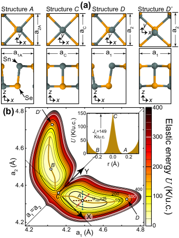
Figure 1: (a) SnSe ML u.c. for points $A$, $C$, $D$, and $D^{\prime}$ on an analytical $U(a_{1},a_{2})$ [subplot (b)]. The solid curve connecting points $A$, $C$, and $B$ on subplot (b) is the minimum-energy pathway among the two energy degenerate basins $A$ and $B$, and the inset displays the energy barrier $J_{C}=U(a_{C},a_{C})$. Straight lines passing through point $A$ were used to determine zero-$T$ elastic moduli. Some isoenergy lines were drawn, too.

Group-IV monochalcogenide monolayers (MLs) are experimentally available [1, 2, 3] 2D ferroelectrics with a puckered rectangular u.c. and a Pnm2₁ group symmetry in their zero-$T$ phase, whereby each atom is threefold coordinated [4, 5, 6, 7, 8, 9, 10, 11, 12, 13]. They display metavalent bonding [14], characterized by large atomic effective charges, structural anharmonicity, and significant linear and non-linear optical responses. Their low-$T$ crystal structure also underpins anisotropic elasticity [15, 16]. Nevertheless, these 2D materials undergo a firmly established structural change onto a fivefold coordinated square structure with P4/nmm symmetry at a critical temperature $T_{c}$ ranging between 200 and 300 K [1, 2, 3, 10, 11, 13], at which their properties turn isotropic. Nothing has been said about the elastic behavior on their P4/nmm phase yet, and approaches based on (i) an analytical form of the zero$-T$ elastic energy landscape [17], and (ii) the strain-fluctuation method [18] are deployed to answer this open question here.

Numerical methods. The elastic energy landscape and MD data were calculated with the SIESTA DFT code [19, 20] employing an exchange correlation functional with self-consistent van der Waals corrections [21]. Additional details can be found in Ref. [10].

Elasticity from elastic energy landscape. As illustrated on Fig. 1(a) for a SnSe ML (a paradigmatic group-IV monochalcogenide ML), a crystal elongated or compressed along two orthogonal directions $a_{1}$ and $a_{2}$ with a subsequent structural optimization of atomic positions for a given value of $a_{1}$ and $a_{2}$ leads to a zero$-T$ elastic energy $E(a_{1},a_{2})$ per u.c. The change of energy $U(a_{1},a_{2})=E(a_{1},a_{2})-E(a_{1A},a_{2A})$ with respect to a degenerate local minimum energy configuration—labeled $A$ and having coordinates $a_{1A}$ and $a_{2A}$—seen on Fig. 1(b) is an elastic energy landscape [22]. To simplify an eventual extraction of partial derivatives, the landscape $U(a_{1},a_{2})$ in Fig. 1(b) is an analytical fit to raw ab initio data [10]. The raw data sets an energy barrier separating the two degenerate minima equal to $J_{C,r}=149.25$ K/u.c., lattice parameters $a_{1A,r}=4.4873$ Å, $a_{2A,r}=4.3264$ Å at the energy minima $A$, and $a_{C}=4.3590$ Å at for the square u.c. of lowest energy [10, 23].

$U(a_{1},a_{2})$ is mirror symmetric with respect to the $a_{1}=a_{2}$ line on Fig. 1(b), thus calling for new variables:

$$X=(a_{1}-a_{2})/\sqrt{2},\text{ and }Y=(a_{1}+a_{2}-2a_{C})/\sqrt{2}.$$ (1)

$X=0$ and $Y=0$ at point $C$ (whose coordinates are $a_{1}=a_{2}=a_{C}$) which thus becomes the new origin of coordinates.

The mirror symmetry of the landscape about the $X=0$ line makes $U(X,Y)$ even on $X$, and the following expression was used to fit numerical data [10]:

$$U(X,Y) =J_{C}+\mathcal{U}_{1}X^{2}+\mathcal{U}_{2}Y^{2}+\mathcal{U}_{3}YX^{2}$$

$$+\mathcal{U}_{4}Y^{3}+\mathcal{U}_{5}X^{4}+\mathcal{U}_{6}Y^{4}$$

$$+(\mathcal{U}_{7}Xe^{-\sqrt{X^{2}}/g_{1}} +\mathcal{U}_{8}YXe^{-\sqrt{X^{2}}/g_{2}})\text{tanh}(100X),\$$

with parameters and numerical uncertainties provided in Table 1. With the exception of the terms on tanh($100X$)—whose sole purpose is to smooth the cusp observed at the barrier in the numerical data [10]; see inset of Fig. 1(b)—the elastic energy landscape is a polynomial of order four. The quality of the fitting can be ascertained by noticing that its minima $A$ is located at $(a_{1A},a_{2A})=(4.4896\text{ \AA},4.3173\text{ \AA})$ [or $X_{A}=0.1218$ Å, $Y_{A}=0.0629$ Å], which is less than 0.25% different from the raw ab initio data. One also notices that the saddle point on $U(X,Y)$ (i.e., the minimum energy barrier separating the two ground states $A$ and $B$) occurs exactly at point $a_{C}$ as determined in the raw data, and that $U(X_{A},Y_{A})=0.0245$ K/u.c., leading to an energy barrier of 148.9755 K/u.c. which is only 0.2745 K/u.c. smaller than the one seen from the raw data.

Zero$-T$ elastic moduli $C_{11}^{(0)}$, $C_{22}^{(0)}$ and $C_{12}^{(0)}$ are customarily obtained by fitting $U(a_{1},a_{2})$ to parabolas [15, 16]:

$$U\simeq\mathfrak{U}=\frac{1}{2}\boldsymbol{\epsilon}^{T}\mathcal{C}^{(0)}\boldsymbol{\epsilon}=\frac{C_{11}^{(0)}\epsilon_{1}^{2}}{2}+\frac{C_{22}^{(0)}\epsilon_{2}^{2}}{2}+C_{12}^{(0)}\epsilon_{1}\epsilon_{2},$$ (3)

where strain coordinates $\boldsymbol{\epsilon}=(\epsilon_{1},\epsilon_{2})^{T}$ with

$$\epsilon_{1}=(a_{1}-a_{1A})/a_{1A},\text{ }\epsilon_{2}=(a_{2}-a_{2A})/a_{2A},$$ (4)

were employed. We recall that $a_{1A}$ and $a_{2A}$ in Eqn. (4) are zero$-T$ equilibrium lattice parameters defining point $A$ in the elastic energy landscape.

$\mathcal{C}^{(0)}$ is the harmonic approximation to the elasticity tensor, and $\mathfrak{U}$ is the harmonic approximation to $U$. As acutely seen in Fig. 2(a), the prescription within Eqn. (3) neglects the strong anharmonicity of group-IV monochalcogenide MLs by definition. Further, given that elastic moduli are thermodynamical averages after all, such approach misses a finite-$T$ understanding of elasticity altogether.

Table 1: Fitting parameters for $U(X,Y)$. $J_{C}=149$ K/u.c.

$\mathcal{U}_{1}$	$-$3660.5 $\pm$ 12.3% K/Å2	$\mathcal{U}_{2}$	24849 $\pm$ 4.3% K/Å2
$\mathcal{U}_{3}$	$-$109410 $\pm$ 8.2% K/Å3	$\mathcal{U}_{4}$	$-$42945 $\pm$ 21.2% K/Å3
$\mathcal{U}_{5}$	188100 $\pm$ 9.2% K/Å4	$\mathcal{U}_{6}$	114840 $\pm$ 43.4% K/Å4
$\mathcal{U}_{7}$	$-$3568.5 $\pm$ 13.4% K/Å	$\mathcal{U}_{8}$	$-$88140 $\pm$ 12.4% K/Å2
$g_{1}$	0.0583 $\pm$ 9.3% Å	$g_{2}$	0.0536 $\pm$ 8.1% Å

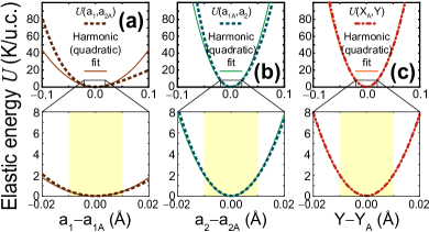
Figure 2: Cuts of $U$ along straight lines passing through point $A$ on Fig. 1(b), and harmonic (i.e., quadratic) fits—thinner solid curves obtained within the shaded regions on the zoom-in plots—from which $C_{11}^{(0)}$, $C_{22}^{(0)}$, and $C_{12}^{(0)}$ were extracted.

$U(X,Y)$ leads to zero$-T$ elastic moduli consistent with prior work [15, 16]: Eqn. (Elasticity of 2D ferroelectrics across their paraelectric phase transformation) is calculated along three straight lines [($a_{1},a_{2A}$), ($a_{1A},a_{2}$), and ($X_{A},Y$), corresponding to the brown (horizontal), green (vertical), and red (at $45^{\circ}$) straight lines passing through point $A$ on Fig. 1(b), respectively] and Eqn. (3) is fitted against the parabolas displayed on Fig. 2. $C_{ij}^{(0)}$ are listed in Table 2 ($i,j=1,2$). Discrepancies with previous results (such as the smaller magnitude of $C_{11}^{(0)}$ and the slightly larger value of $C_{12}^{(0)}$ than $C_{11}^{(0)}$ here) are due to the use of different computational tools and exchange-correlation functionals in ab initio calculations. The softer $C_{11}^{(0)}$ here leads to a smaller $T_{c}$ when contrasted to results using the numerical methods of Refs. [16, 15]; see Refs. [11] and [13] for a discussion.

Table 2: Zero$-T$ in-plane elastic moduli (N/m).

Elastic modulus	Prior work	This work
$C_{11}^{(0)}$	19.9 [15], 19.2 [16]	12.7
$C_{22}^{(0)}$	44.5 [15], 40.1 [16]	51.8
$C_{12}^{(0)}$	18.6 [15], 16.0 [16]	20.9

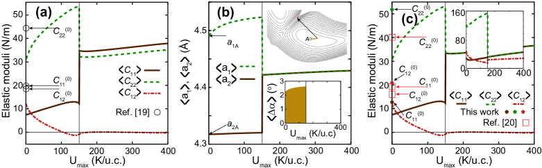
Figure 3: (a) Elastic moduli as a function of $U_{max}-$isovalue, setting the strain with respect to $a_{1A}$ and $a_{2A}$ at zero$-T$. (b) Average lattice constants versus $U_{max}$: the u.c. turns from a rectangle ($\langle a_{1}\rangle>\langle a_{2}\rangle$) onto a square ($\langle a_{1}\rangle=\langle a_{2}\rangle$) when $U_{max}\geq J_{C}$. Insets: evolution of $\langle\Delta\alpha\rangle$ and of the point $(\langle a_{1}\rangle,\langle a_{2}\rangle)$ versus $U_{max}$. (c) Elastic moduli versus $U_{max}$, setting the strain with respect to $\langle a_{1}\rangle$ and $\langle a_{2}\rangle$ as obtained at subplot (b): $\langle C_{11}\rangle=\langle C_{22}\rangle$ are now identical past $J_{C}$. Inset: elastic moduli within the strain-fluctuation method. $C_{11}^{(0)}$, $C_{22}^{(0)}$, and $C_{12}^{(0)}$ as estimated by us and others are shown in subplots (a) and (c).

To go beyond the zero$-T$ paradigm, we make use of $U(X,Y)$ to determine elastic behavior next. A function of $X$ and $Y$ has an expectation value within the elastic energy landscape $\langle f(U_{max})\rangle$ as an average over classically accessible states [17]:

$$\langle f(U_{max})\rangle=\frac{\oint e^{-U(X,Y)/U_{max}}f(X,Y)dXdY}{\oint e^{-U(X,Y)/U_{max}}dXdY},$$ (5)

with $dXdY$ an area element within the confines of a isoenergy contour $U_{max}$ around structure $A$, like those seen on Fig. 1(b).

Within this paradigm, $U(X,Y)$ is a classical potential energy profile, and a set of accessible crystalline configurations lies within isoenergy confines. [$U_{max}$ is the largest kinetic energy of a hypothetical particle in the landscape, and is thus indirectly linked to $T$ that way.] For example, sampled u.c.s will all have $a_{1}>a_{2}$ when the $U_{max}$ isoenergy curve is smaller than $J_{C}$. This is, the sampled structures will all be ferroelectric, having an in-plane polarization along the $x-$direction [10]; see structure $A$ on Fig. 1(a). When $U_{max}\geq J_{C}$ nevertheless, the average structure encompasses minima $A$ and $B$ yielding $a_{1}=a_{2}$, and it thus is a square. The fact that $a_{1}=a_{2}$ on average when $U_{max}\geq J_{C}$ is illustrated by structures $D$ and $D^{\prime}$ on Fig. 1(b), which have $x-$ and $y-$coordinates swapped. In this sense, the averaging among crystalline configurations within the energy landscape up to an energy $U_{max}$ achieves an effect similar to $T$: a transformation whereby the average u.c. turns from a rectangle onto a square. A caveat to this model is that it is based on averaging over independent crystalline u.c.s, while 2D structural transformations in 2D are driven by disorder [8, 9].

Energy average values for $C_{ij}$ are determined by [17]:

$$\langle C_{ij}(U_{max})\rangle= k_{B}\bigg{\{}\bigg{\langle}\frac{\partial^{2}u}{\partial\epsilon_{i}\partial\epsilon_{j}}\bigg{\rangle}$$ (6)

$$-\frac{1}{U_{max}}\bigg{[}\bigg{\langle}\mathcal{A}\frac{\partial u}{\partial\epsilon_{i}}\frac{\partial u}{\partial\epsilon_{j}}\bigg{\rangle}- \langle\mathcal{A}\rangle\bigg{\langle}\frac{\partial u}{\partial\epsilon_{i}}\bigg{\rangle}\bigg{\langle}\frac{\partial u}{\partial\epsilon_{j}}\bigg{\rangle}\bigg{]}\bigg{\}},$$

with $k_{B}$ Boltzmann’s constant, $\mathcal{A}=a_{1}a_{2}$, and $u=U/\mathcal{A}$.

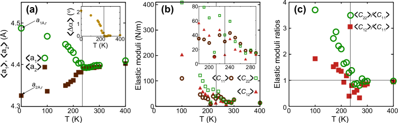
Figure 4: (a) $\langle a_{1}\rangle$ and $\langle a_{2}\rangle$ versus $T$ on MD calculations. Inset: $\langle\Delta\alpha\rangle$. (b) Elastic moduli from the strain-fluctuation method and $\langle\epsilon_{i}\epsilon_{j}\rangle$, $\langle\epsilon_{i}\rangle$ ($i=1,2$) determined from MD: see the coalescence of $\langle C_{11}\rangle$ and $\langle C_{22}\rangle$ past $T_{C}$, and the similar magnitudes of $\langle C_{ij}\rangle$ to those seen at the inset of Fig. 3(c). (c) Ratio among the elastic moduli displayed in subplot (b).

Eqn. (6) was evaluated numerically for energy isovalues $U_{max}$ starting at 1K/u.c and up to 400 K/u.c. [Fig. 3(a)]. Near $U_{max}=0$, the averaging procedure yields elastic moduli smaller than those listed in Table 2. Within this method, $\langle C_{12}\rangle$ quickly decays to a nearly zero value and it becomes negative (for an auxetic behavior). On the other hand, $\langle C_{22}\rangle>\langle C_{11}\rangle$ by a factor in between 3 and 5 for energies up to $U_{max}=J_{C}$, at which a sharp change occurs whereby $\langle C_{22}\rangle\approx\langle C_{11}\rangle$.

The fact that $\langle C_{22}\rangle\neq\langle C_{11}\rangle$ for isovalues $U_{max}\geq J_{C}$, in which the average structure already turned isotropic [see Fig. 3(b)], represents an inaccuracy of the approach in Ref. [17]. It originates from the fact that strain was written out with respect to the zero$-T$ ground state structure ($a_{1A},a_{2A}$) in Eqn. (4). Experimentally, strain at finite$-T$ is measured with respect to a structure in thermal equilibrium, calling for a calculation of elastic moduli in which average values of $a_{1}$ and $a_{2}$ are employed. Strain is then redefined as:

$$\epsilon_{1}=\frac{a_{1}-\langle a_{1}\rangle}{\langle a_{1}\rangle},\text{ and }\epsilon_{2}=\frac{a_{2}-\langle a_{2}\rangle}{\langle a_{2}\rangle},$$ (7)

which is still valid at zero$-T$ in which $\langle a_{i}\rangle=a_{iA}$ ($i=1,2$) The resulting elastic parameters are shown in Fig. 3(c). Now, $\langle C_{22}\rangle=\langle C_{11}\rangle$ for isovalues $U_{max}\geq J_{C}$. The use of Eqn. (7) instead of Eqn. (4) is thus a correction to our previous method [17].

$\langle C_{12}\rangle$ is the softest elastic modulus on this model. On the other hand, $\langle C_{11}\rangle$ hardens significantly at the transition ($U_{max}=J_{C}$), while $\langle C_{22}\rangle$ suddenly softens at $U_{max}=J_{C}$. According to Fig. 3, a SnSe ML is much softer than graphene, for which $C_{11}^{(0)}=C_{22}^{(0)}=336$ N/m, and $C_{12}^{(0)}=75$ N/m (see Ref. [24], and multiply by half of Bernal graphite’s unit cell thickness $\simeq$3.4 Å).

We propose—by direct comparison among $J_{C}$ and $T_{C}$ from numerical calculations [11]—a linear correspondence among these two variables ($T\propto 1.42U_{max}$) for this material, such that $T_{C}=212$ K, and finite$-T$ elastic behavior can be extracted from Fig. 3 at a low computational cost.

Elasticity from the strain-fluctuation method. We next employ the strain-fluctuation method to determine the elastic moduli. The expression to work with is [18]:

$$\langle C^{-1}{}_{ij}\rangle=\frac{\langle\mathcal{A}\rangle}{k_{B}T}\left(\langle\epsilon_{i}\epsilon_{j}\rangle-\langle\epsilon_{i}\rangle\langle\epsilon_{j}\rangle\right),$$ (8)

which is less convoluted than Eqn. (6), and also amenable for MD input.

Computed using $U(X,Y)$, $\langle\epsilon_{i}\rangle=\frac{\langle a_{i}-\langle a_{i}\rangle\rangle}{\langle a_{i}\rangle}=\frac{\langle a_{i}\rangle-\langle a_{i}\rangle}{\langle a_{i}\rangle}=0$ ($i=1,2$) for additional simplification, and $\langle C_{ij}\rangle$ ($i,j=1,2$) are displayed as an inset on Fig. 3(c). One notes that $\langle C_{ij}\rangle>0$ now, so that auxetic behavior cannot be confirmed within the strain-fluctuation method. A second point to notice is that $\langle C_{22}\rangle$ now becomes three times larger than its biggest magnitude obtained using Eqn. 6. For $U_{max}<J_{C}$, $\langle C_{11}\rangle$ is about twice as large than its magnitude from Eqn. 6, too. $\langle C_{11}\rangle=\langle C_{22}\rangle$ for $U_{max}\geq J_{C}$, with a magnitude now comparable to that obtained from Eqn. 6. The two takeouts from the strain-fluctuation approach [inset on Fig. 3(c)] are that $\langle C_{22}\rangle$ is much larger than its estimate using partial derivatives of $U(X,Y)$, and that $\langle C_{21}\rangle$ remains larger than zero.

The Pnm2₁ to P4/nmm structural transformation is signaled by a collapse of the rhombic distortion angle $\langle\Delta\alpha\rangle$ [related to $a_{1}$ and $a_{2}$ as $\langle\Delta\alpha\rangle=\left(\langle\frac{a_{1}}{a_{2}}\rangle-1\right)\frac{180^{\circ}}{\pi}$] to a zero value [1, 10]. As seen at an inset on Fig. 3(b), $U(X,Y)$ does yield the required collapse of $\langle\Delta\alpha\rangle$, but it does not display a gradual decrease with a critical exponent of 1/3 [1, 10] as the inset on Fig. 4(a)—obtained from MD—does. This is so because $U(X,Y)$ makes $\langle a_{1}\rangle$ plow to larger values while $\langle a_{2}\rangle$ remains relatively unchanged up to $U_{max}=J_{C}$, when both lattice parameters change discontinuously onto an identical value [see Fig. 3(b) and its upper inset].

And thus, while an estimation of elastic properties based on $U(X,Y)$ [using either Eqn. (6), or Eqn. (8)] is relatively inexpensive, MD data was also utilized to estimate $\langle C_{11}\rangle$, $\langle C_{22}\rangle$, and $\langle C_{12}\rangle$ within the strain-fluctuation approach. Briefly, 16$\times$16 supercells containing 1024 atoms were employed on NPT ab initio MD calculations for sixteen different $T$s in between 100 and 400 K. 20,000 individual timesteps with a 1.5 fs resolution were obtained for any given $T$. Thermal averages were obtained for times above 5 ps to allow for proper thermalization. In this approach, $\epsilon_{i}=\frac{1}{2}\left[(\langle h\rangle^{-1T}h^{T}h\langle h\rangle^{-1})_{ii}-1\right]$ ($i=1,2$) [18]. $h=(\mathbf{a}_{1},\mathbf{a}_{2})$, and $\langle h\rangle=(\langle\mathbf{a}_{1}\rangle,\langle\mathbf{a}_{2}\rangle)$ are $2\times 2$ matrices containing the in-plane magnitudes of supercell lattice vectors $\mathbf{a}_{1}$ and $\mathbf{a}_{2}$, which are written in column form. The matrix $h$ contains the in-plane superlattice constants for one MD step, and $\langle h\rangle$ is its average over the available MD steps past thermalization. Here, $\langle\mathcal{A}\rangle$ is replaced by the supercell’s area thermal average.

The results, shown in Figs. 4(b) and 4(c), indicate a magnitude of $\langle C_{22}\rangle$ comparable with that of graphene at 100 K [24], but a softer magnitude of $\langle C_{11}\rangle$ that is four times smaller, as it is expected due to the SnSe ML’s anisotropy. All elastic constants then decrease, in a manner similar to that seen at the inset of Fig. 3(c). $\langle C_{ii}\rangle$ ($i=1,2$) turn similar despite of method employed at energies/temperatures above the transition.

Conclusion. The finite$-T$ elastic behavior of a paradigmatic 2D ferroelectric was estimated from second-order partial derivatives of the energy on their zero$-T$ elastic energy landscape, and following the prescriptions of the strain-fluctuation method as well. Within the later method, average strain was introduced utilizing either the elastic energy landscape, or dedicated ab initio MD data. Despite of method, $\langle C_{11}\rangle$ are shown to coalesce past the transition energy $J_{C}$ or temperature $T_{C}$, and the elastic moduli turns much softer than that determined on graphene. The results contained here thus show how to understand the finite-$T$ elastic behavior of 2D materials undergoing two-dimensional transformations.