A Unified Framework for Rank-based Evaluation Metrics for Link Prediction in Knowledge Graphs

Abstract.

The link prediction task on knowledge graphs without explicit negative triples in the training data motivates the usage of rank-based metrics. Here, we review existing rank-based metrics and propose desiderata for improved metrics to address lack of interpretability and comparability of existing metrics to datasets of different sizes and properties. We introduce a simple theoretical framework for rank-based metrics upon which we investigate two avenues for improvements to existing metrics via alternative aggregation functions and concepts from probability theory. We finally propose several new rank-based metrics that are more easily interpreted and compared accompanied by a demonstration of their usage in a benchmarking of knowledge graph embedding models.

1. Introduction

KG are a structured formalism for representing facts about entities $\mathcal{E}$ and their relationships $\mathcal{R}$ as triples of the form $(h,r,t)\in\mathcal{E}\times\mathcal{R}\times\mathcal{E}$. KG are useful for entity clustering, link prediction, entity disambiguation, question answering, dialogue systems, and recommendation systems (Wang et al., 2017). They can be constructed under one of two assumptions: under the CWA, the non-existence of a triple in the KG implies its falsiness and under the OWA, the non-existence of a triple in the KG neither implies its falsiness nor truthiness. Most real-world KG are constructed under the OWA to reflect their relative incompleteness with respect to true triples and typical lack of triples known to be false.

Link prediction on KG constructed under the OWA is a popular approach for addressing their relative incompleteness that can be conceptualized as a binary classification task on triples. However, the lack of false triples leads to a positive unlabeled learning scenario (Bekker and Davis, 2020) which requires negative sampling i.e., randomly labeling some unknown triples as false during the training and evaluation of machine learning models like KGEM. Partially because these techniques introduce bias to classification metrics whose formulation depends on true negatives and false negatives (such as the accuracy, $F_{1}$, and ROC-AUC), the last ten years of KGEM literature has nearly exclusively used the rank-based evaluation metrics: HK, MR, and MRR.

Despite their ubiquity, these metrics are not comparable when applied to datasets of different sizes and properties and lack a corresponding theoretical framework for describing their properties and shortcomings. For example, there is recent interest in applying link prediction with KGEM to real-world tasks in biomedicine such as drug repositioning, target identification, and side effect prediction. However, there are several choices of biomedical KG for training and evaluation, each formulated with different entities, relations, and source databases (Bonner et al., 2021). Because the choice of KG can meaningfully impact downstream applications, hyperparameter search and evaluation must also consider and compare different KG, which, without rank-based evaluation metrics that are comparable across datasets nor theory to help articulate the issue, is not possible.

This work addresses these limitations by making the following contributions: (1) Proposes a theoretical foundation for rank-based evaluation metrics; (2) Proposes and characterizes novel rank-based evaluation metrics with alternative rank transformations and alternative aggregation operations based on special cases of the generalized power mean (Bullen, 2003); (3) Derives probabilistic adjustments for existing and novel rank-based evaluation metrics inspired by (Berrendorf et al., 2020; Tiwari et al., 2021). We implemented the proposed novel metrics and made them available as part of the PyKEEN (Ali et al., 2021) software package.

2. Background

2.1. Generating Ranks

Given a set of entities $\mathcal{E}$, a set of relations $\mathcal{R}$, a KG $\mathcal{K}\subseteq\mathcal{E}\times\mathcal{R}\times\mathcal{E}$, disjoint testing and validation triples $\mathcal{T}_{test},\mathcal{T}_{eval}\subseteq\mathcal{K}$, and a KGEM with scoring function $g:\mathcal{E}\times\mathcal{R}\times\mathcal{E}\rightarrow\mathbb{R}$ (e.g., TransE (Bordes et al., 2013) has $g(h,r,t)=-\|\mathbf{e}_{h}+\mathbf{r}_{r}-\mathbf{e}_{t}\|_{2}$), evaluation concurrently solves two tasks as described by (Nickel et al., 2015):

1. In right-side prediction, for each triple $(h,r,t)\in\mathcal{T}_{eval}$, we score candidate triples $\{(h,r,e)\mid e\in\mathcal{E}\}$ using $g$.

2. In left-side prediction, for each triple $(h,r,t)\in\mathcal{T}_{eval}$, we score candidate triples $\{(e,r,t)\mid e\in\mathcal{E}\}$ using $g$.

In each task, candidate triples are sorted in descending order based on their scores, and are then assigned a rank based on their 1-indexed sort position. In the (optional) filtered setting proposed by (Bordes et al., 2013), candidate triples appearing in $\mathcal{T}_{test}$ are removed from the ordering so they do not artificially increase the ranks of true triples ($\mathcal{T}_{eval}$) appearing later in the sorted list. A good model results in low ranks $r_{1},\dots,r_{n}$ for the true triples, reflecting its ability to assign high scores to true triples and low scores to negatively sampled triples. The ranks are typically aggregated using a rank-based evaluation metric to quantify the performance of the KGEM with a single number.

While the upper bound on an individual rank $r_{i}$ is generally $|\mathcal{E}|$ for both the right- and left-side prediction tasks, the number of candidates may be (considerably) smaller than $|\mathcal{E}|$, e.g., in the filtered setting (Bordes et al., 2013) or during sampled evaluation (Teru et al., 2020; Hu et al., 2021).

2.2. Aggregating Ranks

While the distribution of raw ranks gives full insight into evaluation performance, it is much more convenient to report aggregate statistics. In this subsection, we introduce and describe three common rank-based metrics reported in applications and evaluation of link prediction: HK, MR, and MRR.

HK

The HK (Equation 1) is an increasing metric (i.e., higher values are better) that captures the fraction of true entities that appear in the first $k$ entities of the sorted rank list. Thus, it is tailored towards a use-case where only the top-$k$ entries are to be considered, e.g., due to a limited number of results shown on a search result page. Because it does not differentiate between cases when the rank is larger than $k$, a miss with rank $k+1$ and $k+d$ where $d\gg 1$ have the same effect on the final score. Therefore, it is less suitable for the comparison of different models.

(1) $$\textrm{H}_{k}(r_{1},\ldots,r_{n})=\frac{1}{n}\sum_{i=1}^{n}\mathbb{I}[r_{i}\leq k]\hskip 14.22636pt\in[0,1]$$

where the indicator function $\mathbb{I}$ is defined as $\mathbb{I}[x\leq y]=1$ for $x\leq y$ and $0$ otherwise.

MR

The MR (Equation 2) is a decreasing metric (i.e., lower values are better) that corresponds to the arithmetic mean over ranks of true triples. It has the advantage over HK that it is non-parametric and better reflects average performance.

(2) $$\textrm{MR}(r_{1},\ldots,r_{n})=\frac{1}{n}\sum_{i=1}^{n}r_{i}\hskip 14.22636pt\in[1,\infty]$$

MRR

The MRR (Equation 3) is an increasing metric that corresponds to the arithmetic mean over the reciprocals of ranks of true triples. The construction of the MRR biases it towards changes in low ranks without completely disregarding high ranks like the HK. It can therefore be considered as a soft a version of HK that is less sensitive to outliers and is often used during early stopping due to this behavior. While it has been argued that MRR has theoretical flaws (Fuhr, 2018), these arguments are not undisputed (Sakai, 2020).

(3) $$\textrm{MRR}(r_{1},\ldots,r_{n})=\frac{1}{n}\sum_{i=1}^{n}r_{i}^{-1}\hskip 14.22636pt\in(0,1]$$

2.3. Desiderata

Table 1. Desiderata for rank-based metrics

Property	Constraint	MR	MRR	HK
Non-negativity	$\forall r\in\mathbb{N}:f(r)\geq 0$	✔	✔	✔
Fixed optimum	$f(1)=c_{\text{opt.}}$	✘	✔	✔
Asymp. pessimum	$\lim_{r\to\infty}f(r)=c_{\text{pes.}}$	✘	✔	✔
Anti-monotonic	$r>r^{\prime}\rightarrow f(r)<f(r^{\prime})$	✘	✔	✘
Size invariant	$\mathbb{E}[f]\not\propto n$	✘	✘	✘

After examining the strengths and weaknesses of the three most common rank-based metrics, we outline five desiderata for rank-based metrics that are interpretable and comparable across models/datasets/evaluation tasks in Table 1. Because each of MR, MRR, and HK can be defined with the strictly monotonic increasing arithmetic mean as the aggregation function, we describe our desiderata with respect to the transformation $f$ applied to $r_{i}$ within the aggregation (further explored in subsection 3.1).

We first propose the intuitive constraint that the co-domain of the metric is non-negative, which is satisfied by all three metrics. We next propose that the best rank should result in a fixed optimum (ideally, 1) and that worse ranks should asymptotically approach a fixed pessimum (ideally, 0 for unbalanced metrics and -1 for balanced metrics), which are both satisfied by both MRR and HK but neither by MR.

We propose that along this gradient, the metric should be strictly anti-monotonic, meaning that, as the performance of the KGEM improves, the predictions for true triples should improve, result in lower ranks $r_{i}$, increased values of the transformed ranks $f(r_{i})$, and increased evaluation metrics. This is only satisfied by MRR as MR is an increasing function (i.e., higher ranks result in higher scores) and $f(r_{i})$ for HK has only two discrete values (0 and 1), and thus is not strict in terms of monotonicity.

Because the worst rank is bounded based on the number of candidate triples (which itself depends on the dataset and the evaluation procedure) rather than a constant, the same MR from the evaluation on two different datasets of different sizes should not be directly compared. While MRR and HK are bounded with a constant, the shape of these curves are affected by the same properties of the number of candidate triples and the same issue is applicable. This situation makes the interpretation of results from even large robustness and ablation studies (whose aims are to identify patterns in interaction models, loss functions, regularizations, and other properties of KGEM) challenging at best and misleading at worst. Therefore, our final desideratum is that rank-based metrics should be invariant to the number of candidate triples and directly comparable across different datasets and evaluation procedures.

3. An Analysis of Rank-based Metrics

A general form of a rank-based metric $\mathbb{M}$ over ranks $r_{1},\dots,r_{n}\in\mathbb{N}$ is $\mathbb{M}(r_{1},\ldots,r_{n})=g\big{(}\oplus_{i=1}^{n}f(r_{i})\big{)}$ where $f:\mathbb{N}\mapsto\mathbb{R}$ is a rank transformation function, $\oplus:\mathbb{R}^{n}\mapsto\mathbb{R}$ is an aggregation operation, and $g:\mathbb{R}\mapsto\mathbb{R}$ is a post-aggregation transformation function.

3.1. Insight and Discovery via Transformations

The MR, MRR, and HK metrics use the arithmetic mean as an aggregation function with $\oplus_{i=1}^{n}f(r_{i})=\frac{1}{n}\sum_{i=1}^{n}f(r_{i})$ and varying definitions for rank transformation function $f$ and post-aggregation function $g$ as summarized in Table 2. Based on this formulation, we propose that in addition to the colloquial formulation of MRR using the arithmetic mean and $f(x)=x^{-1}$, it can additionally be formulated with the harmonic mean and $g(x)=x^{-1}$. We suggest a more descriptive name for this metric could be the inverse harmonic mean rank, or IHMR. Considering the definition with the harmonic mean best explains why MRR has the desired properties of an asymptotic pessimum that the MR lacks. It further motivates the construction of two counterpart metrics, the IMR and the HMR (respective inverses of MR and MRR) which are included in Table 2.

Table 2. The identity, reciprocal, and discrete indicator functions are used in combination with various aggregation functions to define the MR, MRR, HK, and four novel metrics. The aggregation (agg.) column uses the $M_{p}$ notation of the generalized Hölder mean described in Appendix Table 3.

Metric	$f(x)$	Agg.	$g(x)$
HK	$\mathbb{I}[x\leq k]$	$M_{1}$	$x$
MR	$x$	$M_{1}$	$x$
MRR	$x$	$M_{-1}$	$x^{-1}$
MRR (colloquial)	$x^{-1}$	$M_{1}$	$x$
IMR	$x$	$M_{1}$	$x^{-1}$
HMR	$x$	$M_{-1}$	$x$
GMR	$x$	$M_{0}$	$x$
IGMR	$x$	$M_{0}$	$x^{-1}$

3.2. Insight and Discovery via Aggregations

While the typical aggregation of ranks applied after various transformations is the arithmetic mean, $\frac{1}{n}\sum_{i=1}^{n}f(r_{i})$, here we present alternate aggregations in Table 3. The max rank and min rank would not be useful in practice due to their susceptibility to outliers, but they nicely demonstrate the bounds on the three Pythagorean means and the quadratic means. Through the lens of the Pythagorean means (i.e., special cases of the generalized Hölder mean in Table 3), we can better explain why MR (and therefore also IMR) tends to bias towards high ranks and MRR (and therefore also HMR) tends to bias towards low ranks. The aggregation that compromises best between the arithmetic mean and harmonic mean is the geometric mean, therefore, we use it to define the GMR and IGMR.

4. Probabilistic Adjustments

Inspired by the probabilistic adjustments to MR that resulted in the AMR and the AMRI (Berrendorf et al., 2020), we considered generalizing their derivations and applying them to MRR and HK. Similar to (Berrendorf et al., 2020), we assume the ranking tasks $i$ to be independent, and the ranks uniformly discretely distributed over $[1,\ldots,N_{i}]$, such that $r_{i}\sim\mathcal{U}(1,N_{i})$. Note that $N_{i}$ may not be constant across ranking tasks $i$ due to filtered evaluation (Bordes et al., 2013).

4.1. Adjustments

Expectation Adjustment. The derivation of the AMR motivated normalizing a base metric $\mathbb{M}$ by its expectation such that $\mathbb{M}^{*}(r_{1},\ldots,r_{n})=\frac{\mathbb{M}(r_{1},\ldots,r_{n})}{\mathbb{E}\left[\mathbb{M}\right]}$. We found that it was only useful for metrics bounded by $[1,\infty)$ (i.e., MR, HMR, GMR) whose adjustments were bounded by $[0,1)$ and not for metrics bounded by $(0,1]$ (i.e., IMR, MRR, IGMR) whose adjustments were unbounded on $(0,\infty)$. The expected value of the adjusted metric is thus $1$. Because it is not generally applicable, we do not propose any new metrics using this adjustment.

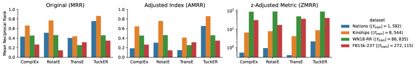
Figure 1. Original, adjusted index, and $z$-adjusted metric for the MRR (inverse harmonic mean rank). Datasets are presented in increasing size from left to right Nations having the least and FB15k-237 having the most.

Adjusted Index. The derivation of the AMRI motivated normalizing a base metric $\mathbb{M}$ by its expectation then linearly transforming it such that the maximum value maps to 1, the expectation maps to 0, positive values can be considered good, and negative values can be considered bad such that $\mathbb{M}^{*}(r_{1},\ldots,r_{n})=\frac{\mathbb{M}(r_{1},\ldots,r_{n})-\mathbb{E}\left[\mathbb{M}\right]}{\max(\mathbb{M})-\mathbb{E}\left[\mathbb{M}\right]}$. We use this form to propose the AHK and AMRR.

Surprisingly, the derivation of AMRI from MR resulted in the same form $\frac{\mathbb{M}-\mathbb{E}[\mathbb{M}]}{1-\mathbb{E}[\mathbb{M}]}$ for the AMRR and the AHK, despite their different monotonicities (i.e., increasing or decreasing) and co-domains. We note that these characteristics do result in different lower bound behavior, which for AMRI is a constant $-1$ and for the AMRR and AHK is a function of the expectation of the base metric $-\frac{\mathbb{E}[\mathbb{M}]}{1-\mathbb{E}[\mathbb{M}]}$. Related derivations can be found in Appendix B.

$z$-Adjustment. We finally propose a novel probabilistic adjustment enabled by the central limit theorem. Because MR, MRR, HK, and other metrics $\mathbb{M}$ are defined as the sum of random variables (despite their several transformations), they have asymptotic Gaussian characteristics. Therefore, we propose using the standarization technique $z=\frac{x-\mu}{\sigma}$ to define a z-scored metric $\mathbb{M}^{*}(r_{1},\ldots,r_{n})=\frac{\mathbb{M}(r_{1},\ldots,r_{n})-\mathbb{E}\left[\mathbb{M}\right]}{\sqrt{\mathbb{V}\mathrm{ar}\left[\mathbb{M}\right]}}$. We apply this to the MR, MRR, and HK to respectively define three new metrics: ZMR, ZMRR, and ZHK. Related derivations can be found in Appendix B.

We note that the z-scored metrics can be monotonically mapped with the cumulative distribution function of the standard normal distribution onto the interval $(0,1)$ to fulfill the desiderata. However, we suggest that z-scores are adequately interpretable and comparable without transformation, as the number of standard deviations below or above of the expected value.

4.2. Discussion

Each of the three probabilistic adjustment strategies presented in this work are affine transformations of the base metric with scale and bias constants only dependent on the studied ranking task, but independent of the investigated predictions. Thus, they can be applied to the base metrics after computation of a pre-computed expectation and variance that are appropriate for the dataset, e.g., to make results from existing publications more comparable across datasets and splits. We provide a database of pre-computed expectations and variances for benchmark datasets included in PyKEEN (Ali et al., 2021) stratified by split (i.e., training, testing, validation), evaluation task (left-hand, right-hand, both), and metric on Zenodo (Hoyt and Berrendorf, 2022).

4.3. Case Study

In order to demonstrate the improved interpretability and comparability of our newly proposed adjustmented metrics and z-scored metrics, we re-evaluated four KGEM (ComplEx (Trouillon et al., 2017), RotatE (Sun et al., 2019), TransE (Bordes et al., 2013), TuckER (Balazevic et al., 2019)) on four datasets (WN18-RR (Dettmers et al., 2018), FB15k-237 (Toutanova and Chen, 2015), Nations, and Kinships (Kemp et al., 2006)) of varying size (from 14 entities to 40k entities, see Appendix Table 4) reusing the optimal hyperparameters reported in (Ali et al., 2020).

Figure 1 presents a comparison between original metric MRR, its adjusted index AMRR, and its $z$-adjustment ZMRR. We first observe that the MRR displays an anti-correlation with size of each dataset that is not present for AMRR and ZMRR, disregarding the smallest dataset for which the numerical behavior of the adjustments is slightly erratic. While the original metric suggests that ComplEx performs similarly on WN18-RR (green) and Nations (blue), the adjusted metric shows that the difference is more remarkable. Conversely, the original metric suggests that TuckER performs better on Nations than WN18-RR, while the adjusted metric shows that when improving comparability by adjusting for size effects, TuckER actually performs better on WN18-RR.

Finally, the $z$-adjusted metric enables direct comparison between the results on different datasets while also giving insight into their significance by normalizing against the expectation and variance of the metric under random rankings. This adjustment reveals that the improved original metrics on the two smaller datasets (Kinships and Nations) were less significant than the results on the two larger datasets (WN18-RR and FB15k-237), despite achieving better unnormalized performance.

All configuration, trained models, results, and analysis presented in this case study are available at https://github.com/pykeen/ranking-metrics-manuscript and archived on Zenodo at (Hoyt et al., 2022).

5. Conclusion

In this article, we motivated and reviewed rank-based evaluation metrics for the link prediction task on KG before proposing desiderata for metrics with improved interpretability and comparability. We developed a simple theoretical framework for describing rank-based evaluation metrics, investigated their probabilistic properties, and ultimately proposed several new metrics with desired properties based on alternate aggregation functions (i.e., HMR, GMR), alternate transformations (i.e., IMR, IGMR), and probabilistic adjustments (i.e., AMRR, AHK, ZMR, ZMRR, and ZHK). We provide implementations of these metrics in PyKEEN (Ali et al., 2021) v1.8.0 with closed form solutions for the expectation and variance of the base metrics when possible and numeric solutions for the rest. We leave the remaining derivations of closed forms for the metrics defined with more complicated functions (e.g., GMR) for future work, to enable generation of z-scored metrics for the remaining base metrics.

Generalization. While we restricted our description in this work to the evaluation of link prediction on KG, the discussed approaches are directly applicable to other settings which use rank-based evaluation, e.g., the entity pair ranking protocol (Wang et al., 2019), entity alignment (Wu et al., 2019; Fey et al., 2020; Sun et al., 2020; Mao et al., 2020), query embedding (Hamilton et al., 2018; Ren et al., 2020; Ren and Leskovec, 2020; Kotnis et al., 2021; Arakelyan et al., 2021; Alivanistos et al., 2022), uni-relational link prediction (Hu et al., 2020; Zhu et al., 2021), and relation detection (Sharifzadeh et al., 2020).

Future Work. Existing evaluation frameworks commonly compute one rank value per evaluation triple and side, then aggregate the ranks. However, real-world KG often contain hub entities that occur in many triples which may therefore dominate the evaluation. We intend to build on previous work (Sharifzadeh et al., 2020; Tiwari et al., 2021; Alivanistos et al., 2022), investigating the issue using our novel metrics in a deeper investigation of rank-based evaluation of the link prediction task on KG.

Appendix A Additional Tables

A.1. Generalized Hölder Mean

Table 3. Aggregation functions formulated with the generalized Hölder (i.e., power) mean $M_{p}(x_{1},\ldots,x_{n})=\sqrt[p]{\frac{1}{n}\sum_{i=1}^{n}x_{i}^{p}}$ as defined in (Bullen, 2003). Note that $\lim_{p\rightarrow 0}M_{p}$ asymptotically approaches the geometric mean.

Name	p	Definition
Max	$+\infty$	$\max\limits_{i}f(r_{i})$
⋮	⋮	⋮
Quadratic Mean	2	$\sqrt[2]{\frac{1}{n}\sum_{i=1}^{n}f(r_{i})^{2}}$
Arithmetic Mean	1	$\frac{1}{n}\sum_{i=1}^{n}f(r_{i})$
Geometric Mean	0	$\sqrt[n]{\prod_{i=1}^{n}f(r_{i})}$
Harmonic Mean	-1	$\big{(}\frac{1}{n}\sum_{i=1}^{n}f(r_{i})^{-1}\big{)}^{-1}$
⋮	⋮	⋮
Min	$-\infty$	$\min\limits_{i}f(r_{i})$

A.2. Datasets

As standard rank-based metrics depend on the number of entities, we chose datasets whose number of entities spanned several orders of magnitudes, from $10^{1}$ to $10^{4}$, for the case study presented in subsection 4.3. We present statistics on these datasets in Table 4.

Table 4. Dataset statistics

Dataset	$|\mathcal{E}|$	$|\mathcal{R}|$	$|\mathcal{T}_{\text{train}}|$
Nations	14	55	1,592
Kinships	104	25	8,544
FB15k-237	14,505	237	272,115
WN18-RR	40,559	11	86,835

Appendix B Derivations of Adjustments

For derivation of the adjustments, we assume each ranking task $r_{i}$ to be independent and identically distributed (i.i.d.) according to a discrete uniform distribution $r_{i}\sim\mathcal{U}(1,N_{i})\in[1,\ldots,N_{i}]$. While the upper bound $N_{i}$ may vary by ranking task $i$, e.g., due to filtered evaluation, we also provide simplified formulas for the case it remains constant throughout the following derivations such that $\forall i:N_{i}=N$. We denote equivalences asserted under this assumption with $\stackrel{{\scriptstyle*}}{{=}}$.

B.1. Adjusting the MR

We begin by briefly recapitulating the derivation of the adjusted (arithmetic) mean rank from (Berrendorf et al., 2020) by first deriving the expectation of the MR (Equation 6). The expectation and variance of a uniformly distributed discrete variable $X\sim\mathcal{U}(a,b)$ are respectively $\mathbb{E}\left[X\right]=\frac{b+a}{2}$ and $\mathbb{V}\mathrm{ar}\left[X\right]=\frac{\left(b-a+1\right)^{2}-1}{12}$. Given our uniformly distributed variable $r_{i}$ with parameters $a=1$ and $b=N_{i}$, we get the following expectation:

(4) $$\mathbb{E}\left[r_{i}\right]=\frac{N_{i}+1}{2}\stackrel{{\scriptstyle*}}{{=}}\frac{N+1}{2}$$

The variance of $r_{i}$ is given as:

(5) $$\mathbb{V}\mathrm{ar}\left[r_{i}\right]=\frac{\left(N_{i}+1-1\right)^{2}-1}{12}\stackrel{{\scriptstyle*}}{{=}}\frac{N^{2}-1}{12}$$

Consequently, the expectation of the MR metric is given as:

(6) $$\mathbb{E}\left[\textrm{MR}\right]=\mathbb{E}\left[\frac{1}{n}\sum\limits_{i=1}^{n}r_{i}\right]=\frac{1}{n}\sum\limits_{i=1}^{n}\mathbb{E}\left[r_{i}\right]=\frac{1}{n}\sum\limits_{i=1}^{n}\frac{N_{i}+1}{2}\stackrel{{\scriptstyle*}}{{=}}\frac{N+1}{2}$$

The variance of the MR metric is given as:

(7) $$\begin{split}\mathbb{V}\mathrm{ar}\left[\textrm{MR}\right]&=\mathbb{V}\mathrm{ar}\left[\frac{1}{n}\sum\limits_{i=1}^{n}r_{i}\right]=\frac{1}{n}\sum\limits_{i=1}^{n}\mathbb{V}\mathrm{ar}\left[r_{i}\right]\\ &=\frac{1}{n}\sum\limits_{i=1}^{n}\frac{N_{i}^{2}-1}{12}\stackrel{{\scriptstyle*}}{{=}}\frac{N^{2}-1}{12}\end{split}$$

B.1.1. Chance-adjusted MR

The chance-adjusted MR (called adjusted mean rank (AMR) in (Berrendorf et al., 2020)) is given as:

(8) $$\textrm{MR}^{*}(r_{1},\ldots,r_{n})=\frac{\textrm{MR}(r_{1},\ldots,r_{n})}{\mathbb{E}\left[\textrm{MR}\right]}\stackrel{{\scriptstyle*}}{{=}}\frac{2}{N(N-1)}\sum_{i=1}^{n}r_{i}$$

B.1.2. Re-indexed Chance-adjusted MR

The authors of (Berrendorf et al., 2020) introduced a re-indexed variant of the AMR named AMRI that is given as follows:

(9) $$\textrm{AMRI}(r_{1},\ldots,r_{n})=1-\frac{MR(r_{1},\ldots,r_{n})-1}{\mathbb{E}\left[\text{MR}-1\right]}\hskip 14.22636pt\in[-1,1]$$

B.2. Adjusting the MRR

The expectation and variance of an inverse-uniform distributed variable $\frac{1}{X}\sim\mathcal{U}\left(\frac{1}{a},\frac{1}{b}\right)$ are $\mathbb{E}\left[\frac{1}{X}\right]=\frac{\ln b-\ln a}{b-a}$ and $\mathbb{V}\mathrm{ar}\left[\frac{1}{X}\right]=\frac{1}{ab}-\big{(}\frac{\ln b-\ln a}{b-a}\big{)}^{2}$. Given our uniformly distributed variable $r_{i}$ with parameters $a=1$ and $b=N_{i}$ and its corresponding inverse-uniform distributed variable $r_{i}^{-1}$, we get the following expectation:

(10) $$\mathbb{E}\left[r_{i}^{-1}\right]=\frac{\ln 1-\ln N_{i}}{N_{i}-1}=\frac{\ln N_{i}}{N_{i}-1}\stackrel{{\scriptstyle*}}{{=}}\frac{\ln N}{N-1}$$

The variance of $r_{i}$ is given as:

(11) $$\mathbb{V}\mathrm{ar}\left[r_{i}^{-1}\right]=\frac{1}{1\cdot N_{i}}-\left(\frac{\ln N_{i}-\ln 1}{N_{i}-1}\right)\stackrel{{\scriptstyle*}}{{=}}\frac{1}{N}-\frac{\ln N}{N-1}$$

The expectation of the MRR metric is given as:

(12) $$\mathbb{E}\left[\textrm{MRR}\right]=\mathbb{E}\left[\frac{1}{n}\sum\limits_{i=1}^{n}r_{i}^{-1}\right]=\frac{1}{n}\sum\limits_{i=1}^{n}\mathbb{E}\left[r_{i}^{-1}\right]=\mathbb{E}\left[r_{i}^{-1}\right]\stackrel{{\scriptstyle*}}{{=}}\frac{\ln N}{N-1}$$

The variance of the MRR metric is given as:

(13) $$\begin{split}\mathbb{V}\mathrm{ar}\left[\textrm{MRR}\right]&=\mathbb{V}\mathrm{ar}\left[\frac{1}{n}\sum\limits_{i=1}^{n}r_{i}^{-1}\right]=\frac{1}{n}\sum\limits_{i=1}^{n}\mathbb{V}\mathrm{ar}\left[r_{i}^{-1}\right]\\ &=\frac{1}{n}\sum\limits_{i=1}^{n}\frac{1}{N_{i}}-\frac{\ln N_{i}}{N_{i}-1}\stackrel{{\scriptstyle*}}{{=}}\frac{1}{N}-\frac{\ln N}{N-1}\end{split}$$

B.2.1. Chance-adjusted MRR

The chance-adjusted MRR is given as:

(14) $$\textrm{MRR}^{*}(r_{1},\ldots,r_{n})=\frac{\textrm{MRR}(r_{1},\ldots,r_{n})}{\mathbb{E}\left[\textrm{MRR}\right]}\stackrel{{\scriptstyle*}}{{=}}\frac{N-1}{N\ln N}\sum_{i=1}^{n}r_{i}^{-1}$$

B.3. Adjusting the HK

The expectation of HK is derived first by deriving the expectation of the discrete indicator function $f(x)=\mathbb{I}\left[x\leq k\right]$ (Equation 15) then applying it in full under the assumption that $N_{i}=N$ for all $i$ (Equation 17). The expectation of $r_{i}$ is given as:

(15) $$\mathbb{E}\left[\mathbb{I}[r_{i}\leq k]\right]=\frac{k}{N_{i}}\stackrel{{\scriptstyle*}}{{=}}\frac{k}{N}$$

The variance of $r_{i}$ is given as:

(16) $$\begin{split}\mathbb{V}\mathrm{ar}\left[\mathbb{I}[r_{i}\leq k]\right]&=\mathbb{E}\left[\mathbb{I}[r_{i}\leq k]\right]\times(1-\mathbb{E}\left[\mathbb{I}[r_{i}\leq k]\right])\\ &=\frac{k}{N_{i}}\times\left(1-\frac{k}{N_{i}}\right)=\frac{k(N_{i}-k)}{N_{i}}\\ &\stackrel{{\scriptstyle*}}{{=}}\frac{k}{N}\times\left(1-\frac{k}{N}\right)=\frac{k(N-k)}{N}\end{split}$$

The expectation of the HK metric is given as:

(17) $$\begin{split}\mathbb{E}[H_{k}]&=\mathbb{E}\left[\frac{1}{n}\sum\limits_{i=1}^{n}\mathbb{I}[r_{i}\leq k]\right]=\frac{1}{n}\sum\limits_{i=1}^{n}\mathbb{E}\left[\mathbb{I}[r_{i}\leq k]\right]\\ &=\frac{1}{n}\sum\limits_{i=1}^{n}\frac{k}{N_{i}}\stackrel{{\scriptstyle*}}{{=}}\frac{k}{N}\end{split}$$

The variance of the HK metric is given as:

(18) $$\begin{split}\mathbb{V}\mathrm{ar}[H_{k}]&=\mathbb{V}\mathrm{ar}\left[\frac{1}{n}\sum\limits_{i=1}^{n}\mathbb{I}[r_{i}\leq k]\right]=\frac{1}{n}\sum\limits_{i=1}^{n}\mathbb{V}\mathrm{ar}\left[\mathbb{I}[r_{i}\leq k]\right]\\ &=\frac{1}{n}\sum\limits_{i=1}^{n}\frac{k(N_{i}-k)}{N_{i}}\stackrel{{\scriptstyle*}}{{=}}\frac{k(N-k)}{N}\end{split}$$

B.3.1. Chance-adjusted HK

The chance-adjusted HK is given as:

(19) $$H_{k}^{*}(r_{1},\ldots,r_{n})=\frac{H_{k}(r_{1},\ldots,r_{n})}{\mathbb{E}\left[H_{k}\right]}=\frac{1}{k}\sum_{i=1}^{n}\mathbb{I}[r_{i}\leq k]$$

B.3.2. Re-indexed Chance-adjusted HK

Combining the facts that ranks are 1-indexed and the $H_{k}\in[0,1]$, the HK can be adjusted as in Equation 20. A negative value of the AHK corresponds to performance below random, zero corresponds to random performance, and 1 to optimal performance. The adjustment for HK is affine with respect to a dataset’s filtering constant, so it can be applied to results after evaluation.

(20) $$AH@k=\frac{H_{k}-\mathbb{E}[H_{k}]}{1-\mathbb{E}[H_{k}]}\hskip 14.22636pt\in\left(-\frac{\mathbb{E}[H_{k}]}{1-\mathbb{E}[H_{k}]},1\right]$$

Note the lower bound was calculated by inserting $\min H_{k}$ as the value for $H_{k}$, which is 0.

B.4. Remaining Adjustments

Identifying a closed-form expectation for the GMR is difficulty because of the inclusion of a product. Further, identifying closed-form expectations for HMR, IGMR, and IMR come from the difficulty of introducing inverses. For these, we implemented a simple workflow to numerically estimate the adjustment constant in PyKEEN that can be applied as an affine transformation after the fact.