Quantum Computation of Reactions on Surfaces Using Local Embedding

Abstract

Modeling electronic systems is an important application for quantum computers. In the context of materials science, an important open problem is the computational description of chemical reactions on surfaces. In this work, we outline a workflow to model the adsorption and reaction of molecules on surfaces using quantum computing algorithms. We develop and compare two local embedding methods for the systematic determination of active spaces. These methods are automated and based on the physics of molecule-surface interactions and yield systematically improvable active spaces. Furthermore, to reduce the quantum resources required for the simulation of the selected active spaces using quantum algorithms, we introduce a technique for exact and automated circuit simplification. This technique is applicable to a broad class of quantum circuits and critical to enable demonstration on near-term quantum devices. We apply the proposed combination of active-space selection and circuit simplification to the dissociation of water on a magnesium surface using classical simulators and quantum hardware. Our study identifies reactions of molecules on surfaces, in conjunction with the proposed algorithmic workflow, as a promising research direction in the field of quantum computing applied to materials science.

1 Introduction

The accurate computational description of correlated electrons in materials is an outstanding research challenge. Quantitative simulations of electronic wavefunctions are essential for accurate and predictive calculations of properties, such as the rates at which industrially relevant or biologically and environmentally hazardous reactions occur. However, it requires a sufficiently accurate solution of an underlying Schrödinger equation. The combinatorial growth of the many-electron Hilbert space, along with the high degree of entanglement produced by electron-electron interaction and Fermi statistics means that the computational cost of exactly solving the Schrödinger equation scales combinatorially with system size, a formidable obstacle that has led to the development of approximate numerical techniques. Methods based on density functional theory (DFT) have had an enormous impact on materials science, but become sensitive to the underlying approximations in presence of static electron correlation [1, 2, 3, 4]. Therefore, a topic of considerable interest is the development of systematic numerical approaches that are chemically realistic and fundamentally many-body.

These approaches include algorithms for quantum computers, which have the potential to accurately and efficiently simulate correlated electronic systems from first principles [5, 6, 7, 8]. Quantum algorithms, based on quantum resource estimates and coupled with classical simulations [9, 10, 11, 12], are projected to deliver results that are competitive with classical methods in both accuracy and cost for specific classes of correlated electronic problems. Common to these problems is the presence of static correlation from electrons and orbitals in a spatially local region, and dynamical correlation from the remaining degrees of freedom.

Many important applications in the electronics, aerospace, automobile, and defense sectors feature a spatially localized region in which electron correlation effects are expected to be more important than in the rest of the system. An example is the corrosion on metallic surfaces, which is initiated by the adsorption of reactants (atoms or molecules from the environment) on a spatially local portion of the surface. In such a situation, it is chemically justified to treat only a portion of the system with an accurate many-body method, and the rest of the system with a less expensive mean-field method. This feature makes reactions on surfaces an especially compelling target for studies on near-term quantum devices, in conjunction with techniques to select relevant degrees of freedom and reduce the budget of quantum simulations.

Here, we propose an algorithmic workflow to simulate reactions on surfaces on quantum computers. The proposed workflow comprises an embedding method specifically designed for reactions of molecules on surfaces, and a circuit simplification technique to facilitate experiments on near-term quantum devices.

First, we developed and compared two methods that are used to rank and select active-space orbitals based on (i) their contribution to the difference between the DFT electronic density of the system and the superimposed DFT electronic densities of the constituent surface and adsorbate and (ii) their effect on the ground-state active-space energy. Second, we solved the Schrödinger equation in the active space using the variational quantum eigensolver [13]. To achieve this goal, it was necessary to evaluate the expectation value of the active-space Hamiltonian over a quantum circuit. We simplified and economized this operation by employing the algebraic properties of Clifford transformations. This allowed for the construction of an equivalent circuit with fewer qubits and gates, and lower depth compared to the original one.

We illustrated the proposed workflow on a step in the corrosion reaction of magnesium by water [14, 15, 16, 17, 18, 19]. We discussed the underlying approximations and assessed their impact on the accuracy of the computed properties. Finally, we demonstrated the proposed workflow using IBM’s quantum hardware.

2 Results

2.1 Chemical Reaction

The corrosion of magnesium in water or aqueous environment proceeds by an electrochemical reaction that produces magnesium hydroxide and hydrogen gas. While the overall corrosion reaction is well-known,

$$\ce{Mg+2H2O<=>>\text{\ce{Mg(OH)2}}+H2}\;,$$ (1)

the detailed mechanisms of hydrogen evolution reactions on a magnesium surface are a topic of ongoing investigation [14, 15, 17, 16, 20].

Williams et al [15] proposed a detailed reaction scheme connecting the steps of initial water dissociation on Mg surface with the final step of $\ce{H_{2}}$ evolution via a Tafel mechanism [21, 15] in the presence of adsorbed OH${}_{\text{ads}}$ and H${}_{\text{ads}}$ species using modeling based on DFT. The suggested reaction mechanism was shown to be a concerted reaction involving multiple water molecules. The first reaction studied in the process was the splitting of a single H_2O molecule creating adsorbed H${}_{\text{ads}}$ and OH${}_{\text{ads}}$ moiety,

$$\ce{Mg+H_{2}O->Mg(OH_{ads})(H_{ads})}\;.$$ (2)

While many steps are involved in the study of the hydrogen evolution process, as discussed in the Supplementary Information (SI), in this work we focused on modeling the chemical reaction in Eq. (2) using the workflow described in Fig. 1. In particular, we computed the electronic energy difference between the reactant and product,

$$\Delta E=E_{\mathrm{product}}-E_{\mathrm{reactant}}\;$$ (3)

Eq. (3) is an important quantity since it is used in the determination of thermodynamic quantities such as the enthalpy or the Gibbs free energy of reaction. In addition to thermodynamics, it is important to characterize the kinetics of surface reaction processes. Determining the kinetics of Eq. (2) involves calculating the activation energy (i.e., the difference between the transition state and reactant energy). Williams et al [15] found that the activation energy for H_2O dissociation on Mg is 1.31 eV for a single H_2O molecule and 1.06 eV for a concerted reaction involving multiple H_2O molecules. Although we did not calculate activation energies in this study, we plan to explore transition states in future research.

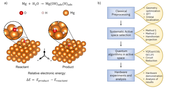
Figure 1: Description of the chemical reaction and the workflow. (a) reaction for splitting of water on a magnesium surface, including schematics of the optimized structures for the reactant and product. (b) Summary of the different steps involved in the workflow. Each step of the workflow is described in detail in the text.

2.2 Classical Pre-processing

The workflow in Fig. 1b starts with classical pre-processing. We obtained optimized geometries of the reactants and products using DFT with periodic boundary conditions (PBC). Schematics of these structures are shown in Fig. 1a. In the optimized structure for the reactant, the water molecule is adsorbed on the surface with the oxygen atom situated 2.4 Å above an atop site. In the optimized structure for the product, the water molecule is split such that OH_ads and H_ads are co-adsorbed at nearest-neighbor fcc sites.

We carried out the simplest PBC calculations at the center of the Brillouin point (${\bf{\Gamma}}$ point), where the Hamiltonian is time-reversal-symmetric. However, ${\bf{\Gamma}}$ point calculations are known to converge slowly and non-monotonically to the thermodynamic limit of infinite system size at zero temperature. To achieve better convergence, in this work, we used twist-averaged boundary conditions (TABC) [22] as an economical alternative to full Brillouin zone sampling [23, 24, 25]. Within TABC, the expectation value of an operator $B$ is averaged over a mesh of $N_{k}$ points ${\bf{k}}_{i}$ in the Brillouin zone, $\langle B\rangle=\frac{1}{N_{k}}\sum_{i=1}^{N_{k}}B({\bf{k}}_{i})$.

At the optimized geometries, we computed the energy difference in Eq. (3) at the DFT level of theory (see Methods). The DFT calculations yielded $\Delta E=-1.91$ eV at the ${\bf{\Gamma}}$ point. By comparison, Williams et al [15] reported $\Delta E=-1.78$ eV. This difference originates from the different optimized geometries, basis sets, and DFT functionals used in the two studies. As a verification, we quantified the basis set superposition error affecting our DFT calculations using the counterpoise correction [26], which yielded $\Delta E_{\mathrm{cp}}=-1.77$ eV, in better agreement with the value obtained by Williams et al in a large plane-wave basis.

To quantify the finite-size error on DFT energies, we performed TABC calculations with $2\times 2\times 1$ and $4\times 4\times 1$ Monkhorst-Pack [27] meshes of ${\bf{k}}$ points, which increased $\Delta E$ by 0.093 and 0.262 eV compared against the ${\bf{\Gamma}}$ point.

2.2.1 Active-Space Selection

For certain chemical problems, reasonably accurate results can be achieved by correlating a limited number of electrons and orbitals through an active-space calculation [28, 29]. In general, an active space of valence electrons and orbitals is most desirable, and further reductions are acceptable when justified by chemical grounds. In particular, all orbitals responsible for static correlation have to be included in the active space [30].

Previous work showed that, for some systems comprising small molecular adsorbates on surfaces, electronic correlation is primarily associated with a limited number of orbitals and electrons [31, 32, 33, 34]. These observations suggest the possibility of constructing compact active spaces for reactions on surfaces. Such a construction should be automated [35, 36] and physics-based. Furthermore, active spaces should be systematically improvable, to allow convergence of computed properties.

In this work, we designed and compared two active-space construction strategies satisfying the above requirements. The starting point of both methods was the separate localization of occupied and virtual DFT orbitals (see Methods), and their projection onto an active region [37] comprising the molecules participating in the reaction and a small portion of the surface.

Method 1 - Based on Density Difference (DD):

This method ranks occupied DFT orbitals according to their contribution to the difference

$$\rho_{\mathrm{DD}}({\bf{x}})=\rho_{\mathrm{Mg+H_{2}O}}({\bf{x}})-\rho_{\mathrm{H_{2}O}}({\bf{x}})-\rho_{\mathrm{Mg}}({\bf{x}})$$ (4)

between the DFT electronic density of the full system and the sum of the DFT electronic densities of adsorbate and slab. More specifically, we multiplied $\sqrt{\rho_{\mathrm{DD}}({\bf{x}})}$ times the absolute value of each localized occupied DFT orbital $|\psi_{i}({\bf{x}})|$, integrated this product over space, and retained the five (as many as the valence occupied orbitals of $\ce{H_{2}O}$) orbitals with the highest integrated overlaps (see also Fig. 2ab and Methods). On the one hand, this method provides a simple and inexpensive way of ranking occupied DFT orbitals. On the other hand, the ranking of virtual DFT orbitals is more subtle, because they do not significantly contribute to Eq. (4). For each retained occupied and virtual DFT orbital, respectively $\psi_{i}$ and $\psi_{a}$, we computed the CCSD (coupled-cluster singles and doubles) energy in a (2e,2o) active space spanned by $\psi_{i}$ and $\psi_{a}$ (see Fig. 2c). It is worth noting that, for two-electron systems, CCSD is exact. We then sorted pairs $(i,a)$ according to the value of the (2e,2o) CCSD energy, and retained the highest-ranking virtual orbitals. This method is efficient in terms of the required classical resources and yields active-space ground-state energies that decrease monotonically with increasing active-space size (see Fig. 2d).

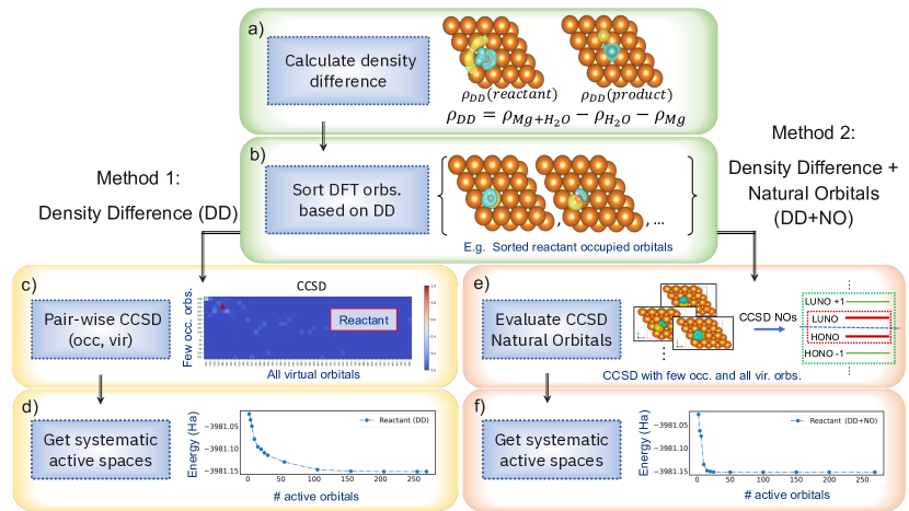
Figure 2: Active-space selection methods based on the electron density difference. The top two blocks (a,b) are common to both methods. The two blocks on the left (c,d) illustrate the steps of the first method, denoted Density Difference (DD). The two blocks on the right (e,f) describe the steps of the second method, denoted Density Difference + Natural Orbitals (DD+NO).

Method 2 - Based on Density Difference and CCSD Natural Orbitals (DD+NO):

As seen in Fig. 2d, the energy converges slowly with active-space size. Convergence improves considerably using natural orbitals [38, 39]. In the DD+NO method, we carried out a CCSD calculation in the active space spanned by the five highest-ranking occupied DFT orbitals (determined as in the DD method) and all virtual orbitals. We then constructed natural orbitals as eigenvectors of the CCSD one-particle density matrix, sorted them in decreasing order of occupation number. For the problems studied here, occupation numbers were either close to 2 or to 0, so we could unambiguously divide orbitals as high- and low-occupancy (in systems with strong correlation, there is a set of natural orbitals with fractional occupation numbers, and it is necessary to include them in the active space). We sorted natural orbitals in decreasing order of occupation number and defined the highest-occupied and lowest-unoccupied natural orbitals (HONO and LUNO respectively) as the orbitals with indices $N_{e}/2$ and $N_{e}/2+1$, where $N_{e}$ is the number of electrons. We then constructed active spaces spanning orbitals between HONO$-a$ and LUNO$+b$ with $a=\min(k,N_{e}/2-1)$ and $b=\min(k,N_{o}-N_{e}/2-1)$ where $k\geq 0$ is an integer and $N_{o}$ the total number of orbitals (see Fig. 2e).

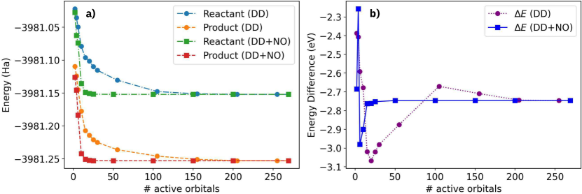
Figure 3: Comparison of active-space selection methods. CCSD total energies (a) and energy differences $\Delta E$ (b) calculated in active spaces constructed with DD and DD+NO methods.

Comparison:

In Fig. 3, we compared DD and DD+NO methods by computing the CCSD total energies of reactant and product (left) and the corresponding energy difference (right) as a function of active-space size (see Methods). We considered active spaces of up to 269 orbitals (5 of which are occupied) out of the 588 orbitals in the underlying Gaussian basis set and evaluated energies and energy differences at the ${\bf{\Gamma}}$ point. DD+NO total energies and energy differences converged faster than their DD counterparts. In particular, only 15-20 natural orbitals are needed to converge $\Delta E$. Therefore, in the remainder of this work, we used active spaces constructed with DD+NO. We remark that, while the DD+NO method offers faster ground-state energy convergence, it is considerably more expensive than the DD method, as it requires correlated calculations, which become challenging for bases of hundreds of orbitals. The DD and DD+NO methods are not mutually exclusive but can be used as complementary approaches, for example, the DD method can be used to rank occupied orbitals and identify a subset of relevant virtual DFT orbitals, that can then be treated with DD+NO.

2.3 Quantum algorithms in the active space

After identifying the active-space orbitals for each ${\bf{k}}$ point, we froze the remaining orbitals and projected the Born-Oppenheimer Hamiltonian onto the active space with a standard procedure [37, 40]. We represented the active-space Hamiltonian in second quantization, and mapped it to a qubit operator using conventional fermion-to-qubit mappings, namely Jordan-Wigner (JW) and parity with two-qubit reduction (P2QR) [41, 42, 43].

2.3.1 Variational Quantum Eigensolver (VQE)

We performed active-space simulations using the VQE method, wherein the ground-state wavefunction and energy, $E_{0}$, are approximated by variationally optimizing a parameterized wavefunction ansatz $|\psi(\boldsymbol{\theta})\rangle$,

$$E_{\mathrm{VQE}}=\min_{\boldsymbol{\theta}}\langle\psi(\boldsymbol{\theta})|H|\psi(\boldsymbol{\theta})\rangle\;.$$ (5)

The function $E_{\mathrm{VQE}}$ is evaluated on a quantum computer, and the parameters $\boldsymbol{\theta}$ are optimized on a classical computer. The quality of a VQE calculation, and particularly the difference $E_{\mathrm{VQE}}-E_{0}$, depends on the VQE ansatz and the convergence of the optimization procedure. Literature [44, 45, 46, 47, 48, 40] indicates that VQE applied to small systems can yield energies close to those of exact diagonalization in the active space, known as complete active space configuration interaction (CASCI).

Here, we studied the performance of the VQE algorithm using a Trotterized implementation of Unitary CCSD (qUCCSD) [45], Entanglement Forging (EF) [49], and Qubit Coupled Cluster (QCC) [50]. See Methods for more information.

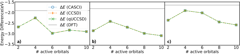
Figure 4: Active-space energy differences. Energy differences $\Delta E$ with CASCI, CCSD, and qUCCSD evaluated over active spaces of 2 to 10 CCSD natural orbitals constructed with the DD+NO method. $\Delta E$ is computed at the ${\bf{\Gamma}}$ point (a) and with TABC over $2\times 2\times 1$ (b) and $4\times 4\times 1$ (c) Monkhorst-Pack grids. DFT energy differences are shown for reference in grey.

We begin our analysis in Fig. 4, where we compare $\Delta E$ from qUCCSD against CCSD and CASCI. We illustrate the impact of going beyond the ${\bf{\Gamma}}$ point (left) via TABC over Monkhorst-Pack grids of $2\times 2\times 1$ (middle) and $4\times 4\times 1$ (right) ${\bf{k}}$ points. qUCCSD, CCSD, and CASCI are indistinguishable for all active-space sizes and ${\bf{k}}$ point meshes. DFT energy differences are also reported for comparison.

The qUCCSD ansatz is accurate but expensive, featuring circuits of depth scaling as $O(N^{4})$, where $N$ is the number of active-space orbitals [51]. This fact motivated the development of ansatzes that reduce computational cost while retaining accuracy. Here, we employed one such ansatz, QCC [50, 52, 53], which applies exponentials of suitably-chosen Pauli operators $P_{1}\dots P_{m}$ (see Methods) to the Hartree-Fock state,

$$|\psi_{\mathrm{QCC}}(\boldsymbol{\theta})\rangle=e^{-i\theta_{m}P_{m}}\dots e^{-i\theta_{1}P_{1}}|\psi_{\mathrm{HF}}\rangle\;.$$ (6)

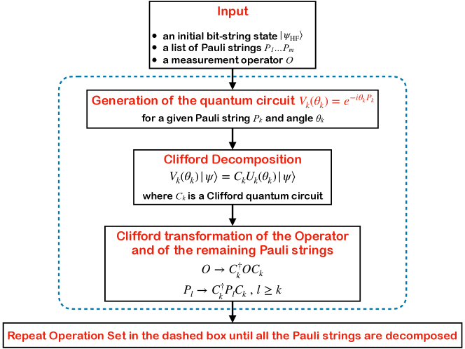
Figure 5: Circuit reduction. Flowchart of the circuit reduction technique for circuits comprising initialization of qubits in a computational basis state $\psi_{\mathrm{HF}}$ (or bitstring), a product of exponentials of Pauli operators $P_{k}$ (or Pauli strings), and the measurement of a Pauli operator $O$.

2.3.2 Circuit reduction

Evaluating the QCC energy requires computing expectation values of Pauli operators $O$ over a state of the form Eq. (6),

$$\langle\psi(\boldsymbol{\theta})|O|\psi(\boldsymbol{\theta})\rangle=\langle\psi_{\mathrm{HF}}|e^{i\theta_{1}P_{1}}...e^{i\theta_{m}P_{m}}|O|e^{-i\theta_{m}P_{m}}...e^{-i\theta_{1}P_{1}}|\psi_{\mathrm{HF}}\rangle\;,$$ (7)

which is challenging on near-term quantum devices due to the high number of qubits, gates, high circuit depth, and limited qubit connectivity. Here, we devised a circuit simplification technique that significantly reduced the quantum resources required for computing Eq. (7).

(i) As a preliminary step, we permuted qubits in the register so that Pauli operators $P_{k}$ act non-trivially, e.g., on the rightmost qubits, prioritizing $P_{k}$ over $P_{k+1}$. (ii) We then represented the state $e^{-i\theta_{1}P_{1}}|\psi_{\mathrm{HF}}\rangle$ as $C_{1}U_{1}(\theta_{1})|0\rangle$, where $C_{1}$ is a Clifford transformation. We constructed $C_{1}$ using a combination of standard circuit identities, such as commuting a Hadamard gate through a CNOT gate [54, 55, 56], as discussed in the SI. (iii) We used $C_{1}$ to perform a similarity transformation on the Pauli operators $P_{2},\dots,P_{m}$, and $O$ without altering the expectation value in Eq. (7),

$$\langle\psi(\boldsymbol{\theta})|O|\psi(\boldsymbol{\theta})\rangle = \langle\psi_{\mathrm{HF}}|e^{i\theta_{1}P_{1}}\dots e^{i\theta_{m}P_{m}}|O|e^{-i\theta_{m}P_{m}}\dots e^{-i\theta_{1}P_{1}}|\psi_{\mathrm{HF}}\rangle$$ (8)

$$= \langle 0|U_{1}^{\dagger}(\theta_{1})e^{i\theta_{2}P_{2}^{\prime}}\dots e^{i\theta_{m}P_{m}^{\prime}}|O^{\prime}|e^{-i\theta_{m}P_{m}^{\prime}}\dots e^{-i\theta_{2}P_{2}^{\prime}}U_{1}(\theta_{1})|0\rangle\;,$$ (9)

where $P^{\prime}_{k}=C_{1}^{\dagger}P_{k}C_{1}$ and $O^{\prime}=C_{1}^{\dagger}OC_{1}$ are Pauli operators that can be determined efficiently [57] on a classical computer. In Eq. (9) we removed the Clifford transformation $C_{1}$ from the quantum circuit executed on hardware by applying similarity transformations to $P_{k}$ and $O$. Thanks to this removal, and the fact that the circuit $U_{1}(\theta_{1})$ has by construction shorter depth and fewer gates than $V_{1}(\theta_{1})$, the simplified circuit has shorter depth and fewer gates than the original one. (iv) we repeated the previous two steps for each Pauli operator in the circuit. At the end of step (iv), we determined whether the reduced circuit acts trivially on one or more qubits, and removed such qubits (if any) from the calculation. A detailed workflow is shown in Fig. 5 and a complete example is shown in the SI.

By applying this technique, the quantum resources to simulate the QCC ansatz are significantly reduced, as exemplified in Table 1 for reactant and product at the $\boldsymbol{\Gamma}$ point.

#Natural	#Pauli	#CNOTs	#CNOTs	Depth	Depth	#Qubits	#Qubits
Orbitals	Strings	(before)	(after)	(before)	(after)	(before)	(after)
2	3	2/2	1/1	18/18	6/6	2/2	2/2
4	25	130/122	39/57	256/248	60/72	6/6	6/6
6	25	180/210	62/86	306/336	70/81	10/10	9/9
8	25	340/346	74/47	466/472	73/61	14/14	11/8
10	25	482/396	72/72	608/522	55/69	18/18	13/13

Table 1: Number of CNOT gates and circuit depth before and after applying the circuit reduction procedure to QCC ansatzes with varying number of Pauli strings (second column), for reactant/product in active spaces of different sizes (first column).

2.3.3 Simulations on quantum hardware

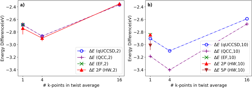
Figure 6: Results from quantum algorithms and hardware experiments. Energy differences $\Delta E$ from noiseless classical simulations and hardware experiments, for active spaces of 2 (a) and 10 (b) natural orbitals from the DD+NO method. For 10-orbital active spaces, we employed QCC with 50 Pauli operators (purple crosses) on classical simulators and QCC with 2 and 5 Pauli operators ($\Delta E~{}2P$ and $\Delta E~{}5P$) on quantum hardware.

In Fig. 6 we simulate VQE with QCC and EF ansatzes, using qUCCSD as a reference due to its high accuracy, established in Fig. 4. We start by considering a (2e,2o) active space spanned by the HONO and LUNO orbitals and $n\times n\times 1$ meshes of ${\bf{k}}$ points with $n=1,2,4$ (left panel). This active space requires 4 and 2 qubits in JW and P2QR representations, respectively (left panel). Noiseless classical simulations show that various ansatzes are in agreement with each other and with qUCCSD. Hardware simulations using QCC with 2 Pauli strings as ansatz (red triangles) are statistically compatible with noiseless classical simulations.

We then consider a (10e,10o) active space spanned by the HONO-4 to LUNO+4 orbitals and $n\times n\times 1$ meshes of ${\bf{k}}$ points with $n=1,2,4$ (right panel). This active space generally requires 20 and 18 qubits in JW and P2QR representations respectively (left panel). On noiseless classical simulators, we employed QCC with 50 Pauli strings. On quantum hardware, we implemented QCC with 2 and 5 Pauli strings. We used the circuit reduction technique outlined in the previous section to achieve more economical simulations. In the case of 2 and 5 Pauli strings, reduced circuits acted on 2 and 5 qubits respectively, and had depth 2. The original circuits required, for the reactant/product systems, are (i) 15/14 qubits, 24/20 CNOT gates, and 35/31 circuit depth for QCC with 2 Paulis and (ii) 17/16 qubits, 64/56 CNOT gates and 85/77 circuit depth for QCC with 5 Paulis. We note that hardware simulations are statistically compatible with noiseless classical simulations using the same quantum circuit. Furthermore, energy differences computed with QCC depend non-trivially on the number of Pauli operators in the ansatz: in particular, simulations using 50 Pauli operators differ from qUCCSD by roughly $0.1$-$0.3$ eV. At the ${\bf{\Gamma}}$ point, we incorporated results from EF for reference. This method can tackle (2e,2o) and (10e,10o) active spaces with 2 and 10 qubits respectively. EF yields results in good agreement with qUCCSD and QCC. However, it should be noted that its current implementation is limited to Hamiltonians with time-reversal symmetry.

Additional information about the performance of the QCC and EF ansatzes is provided in the SI.

3 Discussion

Here, we proposed a workflow to simulate reactions of molecules on surfaces with quantum computing algorithms. The proposed workflow comprises an active-space construction and a circuit simplification to economize quantum simulations and facilitate their demonstration on near-term quantum devices.

Embedding/active-space construction:

Several methods using quantum algorithms as solvers for one or more active regions have been recently proposed, targeting model systems of strong electronic correlation [58] and spin defects in semiconductors and insulators [59, 60, 61]. An important contribution of our study is the design of automated active-space selection techniques specifically tailored for reactions on surfaces. In this situation, electronic correlation arises primarily from a spatially localized region, suggesting the possibility to construct compact active spaces, but the clear identification of such region is non-trivial, especially under the desideratum that the active spaces comprise a few electrons and orbitals. We observed that occupied localized DFT orbitals can be reliably ranked based on their contribution to the difference between the DFT density of the adsorbate+surface complex and the sum of the individual DFT densities of adsorbate and surface, Eq. (4). The ranking and selection of virtual DFT orbitals is more delicate and requires estimating their contribution to the active-space ground-state energy. In line with chemical knowledge [62, 63, 64, 65], we observed that natural orbitals lead to faster convergence of active-space ground-state energies than DFT orbitals, as they can capture anti-bonding virtual orbitals as opposed to the Rydberg continuum [66]. In this work, we used CCSD calculations to construct natural orbitals, which are expensive for large systems. However, this issue can be mitigated by pre-screening virtual orbitals based on the density difference Eq. (4) and/or resorting to less expensive MBPT2 (many-body second-order perturbation theory) calculations for dynamically correlated systems.

Active-space simulations:

In the solution of the Schrödinger equation for the active space, we built upon recent work on the adaptation of quantum algorithms to crystalline solids [67, 47, 68, 69, 70, 71] and the design of variational ansatzes [50, 49] suited for near-term hardware. An important contribution of our study is the introduction of a systematic and automated circuit simplification method based on iterative Clifford transformations. We tested the proposed circuit reduction technique focusing on the QCC ansatz and observed systematic and substantial reductions in the required number of CNOT gates and circuit depth, which stands to benefit simulations, especially on near-term quantum hardware. Although investigated for the QCC ansatz, the circuit reduction technique proposed here is general, as it applies to any situation described by Eq. (7).

Applications and Perspective:

Here, we demonstrated the proposed workflow using a step in the corrosion reaction of magnesium by water as an application. Previous studies have computed electronic and thermodynamic parameters using DFT [14, 15, 16, 17, 18, 19]. Our study is a step towards the refinement of these calculations by (i) selecting a chemically meaningful and systematically improvable active space through an automatic, cost-effective procedure, and (ii) employing many-body methods in combination with an exact, automated, and general-purpose circuit reduction technique to simulate the active space.

The workflow proposed here is a natural choice in studying the adsorption and splitting of water onto a metal surface, which is an example of a broader class of reactions. These reactions include heterogeneous catalysis and atmospheric corrosion of substrates (e.g., surfaces made of transition metals and/or containing defects) by adsorbates (e.g., O₂), and involve bond breaking/formation in spatially localized regions, making them amenable to description through embedding and quantum computing active-space simulations.

Finally, the proposed workflow is valuable for both near- and long-term quantum computers. In the near term, it enables studies of complex chemical phenomena on noisy quantum devices by selecting relevant degrees of freedom and reducing quantum resource requirements. In the long term, it can support the study of systems with strong and spatially local electronic correlation, where traditional methods become less reliable [9, 12, 11], using sophisticated algorithms like quantum phase estimation. Therefore, this workflow indicates a promising direction in the search for advantageous applications of quantum simulation algorithms.

4 Methods

4.1 Geometry Optimization

We performed geometry optimizations using plane-wave bases with Quantum ESPRESSO [72] (QE) v6.3. We modeled the hcp Mg(0001) surface using a slab of 4 Mg layers with 16 atoms per layer, having a thickness of 7.8 Å having 10.5 Å of vacuum separation between periodic images. Mg atoms in the 2 bottom layers were kept fixed in their positions, and those in the 2 top layers were allowed to relax.

We performed calculations with the Perdew-Wang 91 DFT functional [73], the scalar-relativistic Vanderbilt ultra-soft pseudo-potential [74], and a 30/360 Ry cutoff for wavefunction/density plane-wave expansion. We tested Brillouin zone convergence, for the optimized reactant and product geometries, using meshes of up to $8\times 8\times 1$ ${\bf{k}}$ points (see the SI). Results from $4\times 4\times 1$ and $8\times 8\times 1$ meshes are within 1.6 kcal/mol of each other.

4.2 DFT calculations in a Gaussian basis

At the optimized geometries described above, we performed DFT calculations using a single-particle basis of translational-symmetry-adapted linear combinations of Gaussian atomic orbitals (AOs),

$$\varphi_{{\bf{k}},p}({\bf{r}})=\sum_{{\bf{T}}}e^{i{\bf{k}}\cdot{\bf{T}}}\chi_{p}({\bf{r}}-{\bf{T}})\;.$$ (10)

Here, ${\bf{T}}=\sum_{i=1}^{3}T_{i}{\bf{a}}_{i}$ is a lattice translation vector, ${\bf{k}}=\sum_{i=1}^{3}k_{i}{\bf{b}}_{i}$ is a momentum vector in the first Brillouin zone of the lattice, and $\chi_{p}$ is an orbital from a Gaussian basis set. The summation over ${\bf{T}}$ leads to a basis of translational-symmetry-adapted orbitals [75, 23].

We performed DFT calculations with the PySCF package [76, 77]. We used the GTH-DZV basis set [78], the associated Goedecker-Teter-Hutter (GTH) pseudo-potential [78], and the Perdew-Burke-Ernzerhof (PBE) functional [79].

In the basis (10), the Born-Oppenheimer Hamiltonian takes the form [80]

$$\hat{H}=E_{0}+\sum_{\begin{subarray}{c}{\bf{k}}\\ pr\\ \sigma\end{subarray}}h_{pr}({\bf{k}})\hat{a}^{\dagger}_{{\bf{k}}p\sigma}\hat{a}^{\phantom{\dagger}}_{{\bf{k}}r\sigma}+\sum^{*}_{\begin{subarray}{c}{\bf{k}}_{p}{\bf{k}}_{r}{\bf{k}}_{q}{\bf{k}}_{s}\\ prqs\\ \sigma\tau\end{subarray}}\frac{({\bf{k}}_{p}p,{\bf{k}}_{r}r|{\bf{k}}_{q}q,{\bf{k}}_{s}s)}{2}\hat{a}^{\dagger}_{{\bf{k}}_{p}p\sigma}\hat{a}^{\dagger}_{{\bf{k}}_{q}q\tau}\hat{a}^{\phantom{\dagger}}_{{\bf{k}}_{s}s\tau}\hat{a}^{\phantom{\dagger}}_{{\bf{k}}_{r}r\sigma}\;,$$ (11)

where the $*$ symbol indicates crystal momentum conservation, i.e. ${\bf{k}}_{p}+{\bf{k}}_{q}-{\bf{k}}_{r}-{\bf{k}}_{s}={\bf{G}}$, where ${\bf{G}}$ is a reciprocal lattice vector. Here, we approximated the electron-electron interaction with density fitting using a Weigend auxiliary basis.

4.3 Active-Space Selection

Orbital localization:

We localized Kohn-Sham orbitals using Pipek-Mezey method [81, 82, 83] based on a Mulliken population analysis with meta-Löwdin orbitals. [83, 82]. We conducted separate localization for occupied and virtual orbitals, at each ${\bf{k}}$ point individually.

Density difference:

We computed the electronic density difference, Eq. (4), at DFT level. This quantity is shown in the SI for the reactant and product. For each localized DFT orbital $\psi_{\ell}({\bf{x}})$, we computed the overlap function

$$\mathcal{O}_{\ell}({\bf{x}})=\sqrt{\rho_{\mathrm{DD}}({\bf{x}})}\,|\psi_{\ell}({\bf{x}})|$$ (12)

and the integrated overlap

$$\tilde{\mathcal{O}}_{\ell}[\eta]=\int d{\bf{x}}\quad\mathcal{O}_{\ell}({\bf{x}})H(\mathcal{O}_{\ell}({\bf{x}})-\eta)\;.$$ (13)

In Eq. (13), the parameter $\eta$ is a threshold used to truncate the tails of $\mathcal{O}_{\ell}({\bf{x}})$ and $H(x)$ is Heaviside’s step function. For small $\eta$, due to such tails, physically irrelevant orbitals delocalized across the metallic surface have artificially high integrated overlaps. For large $\eta$, all orbitals (including physically relevant ones) have zero integrated overlap. However, there is a broad region of values of $\eta$, that we identified by a simple scan, that leads to a stable ordering of orbitals. We then used integrated overlap $\tilde{\mathcal{O}}_{\ell}[\eta]$ to rank the occupied localized DFT orbitals.

4.4 Variational ansatzes for active-space simulations

Unitary CCSD:

This ansatz is obtained by applying the exponential of the anti-Hermitian operator $T-T^{\dagger}$ to the Hartree-Fock state. $T$ is a linear combination of single and double excitations from occupied (indexed as $j,k$) to virtual spin-orbitals (indexed as $b,c$). More specifically,

$$|\psi_{\mathrm{UCCSD}}(\boldsymbol{\theta})\rangle = e^{T-T^{\dagger}}|\psi_{\mathrm{HF}}\rangle$$ (14)

$$T = T_{1}+T_{2}$$ (15)

$$T_{1} = \sum_{aj}(\theta^{R}_{aj}+i\theta^{I}_{aj})\hat{a}^{\dagger}_{a}\hat{a}^{\phantom{\dagger}}_{j}$$ (16)

$$T_{2} = \sum_{ajbk}(\theta^{R}_{ajbk}+i\theta^{I}_{ajbk})\hat{a}^{\dagger}_{a}\hat{a}^{\dagger}_{b}\hat{a}^{\phantom{\dagger}}_{k}\hat{a}^{\phantom{\dagger}}_{j}\;,$$ (17)

where $\hat{a}^{\dagger}_{a}$/$\hat{a}^{\phantom{\dagger}}_{j}$ creates/destroys an electron at spin-orbital $a$/$j$, and the coefficients $\boldsymbol{\theta}=\{\theta^{R}_{aj}$, $\theta^{I}_{aj}$, $\theta^{R}_{ajbk}$, $\theta^{I}_{ajbk}\}$ are variational parameters. At the ${\bf{\Gamma}}$ point, where the Hamiltonian Eq. (11) is time-reversal-symmetric, electronic eigenfunctions are real-valued and coefficients $\theta^{I}$ can be forced to zero. Away from the ${\bf{\Gamma}}$ point, this is no longer true. To implement the ansatz Eq. (14) on a gate-based quantum computer, we mapped the fermionic operator $T-T^{\dagger}$ onto a linear combination of Pauli operators. Then, we approximated $\exp(T-T^{\dagger})$ with a Trotter-Suzuki approximation or other product formulas, yielding the Trotterized form of UCCSD, known as qUCCSD [45]. We implemented the qUCCSD using Qiskit [84], with appropriate modifications to include the coefficients $\theta^{I}$.

Qubit coupled-cluster:

the QCC ansatz [50, 52] is defined by sequentially applying exponentials of Pauli strings from an ordered set $P_{1}\dots P_{m}$ to the Hartree-Fock state as in Eq. (6). The Pauli operators $P_{k}$ are typically [50, 52] ranked based on the value of the energy gradient $g(P)=|\langle\psi_{\mathrm{HF}}|[H,P]|\psi_{\mathrm{HF}}\rangle|$. The number $m$ is determined based on the convergence of the QCC energy or the budget of the simulator/hardware at hand. In this study, for simplicity, we elected to choose the operators $P_{k}$ based on the coefficients of the CASCI wavefunction $|\psi_{\mathrm{CASCI}}\rangle=\sum_{c}v_{c}|\psi_{c}\rangle$. More specifically, we sorted the configurations $\psi_{c}$ in decreasing order of $|v_{c}|$ and retained the top $m/2$ configurations. For each such configuration, we constructed two Pauli operators $P_{c},Q_{c}$ such that $P_{c}|\psi_{\mathrm{HF}}\rangle=|\psi_{c}\rangle$ and $Q_{c}|\psi_{\mathrm{HF}}\rangle=i|\psi_{c}\rangle$, and introduced them in the pool of QCC Pauli operators. We implemented the QCC ansatz using Qiskit and optimized it with the L_BFGS_B [85] algorithm on noiseless classical simulators.

Entanglement Forging:

this algorithm [49] writes a wavefunction $\Psi$ of a bipartite quantum system $A+B$ through a Schmidt decomposition,

$$|\Psi_{\mathrm{A}+\mathrm{B}}\rangle=\sum_{i=1}^{R}\lambda_{i}U|x_{i}\rangle\otimes V|y_{i}\rangle\;.$$ (18)

In Eq. (18), $U$ and $V$ are unitary matrices, $\lambda_{i}$ are Schmidt coefficients, and $x_{i},y_{i}$ are computational basis states (or bitstrings). The number $R$ is called the Schmidt rank of $\Psi_{\mathrm{A}+\mathrm{B}}$, and depends on the entanglement across $A$ and $B$. Operators like the Hamiltonian are written as linear combinations $H=\sum_{a,b=1}^{h}w_{a,b}P_{a}\otimes P_{b}$ of Pauli operators acting on $A$ and $B$ individually, and its expectation value over $\Psi_{\mathrm{A}+\mathrm{B}}$ is written as

$$E=\sum_{\begin{subarray}{c}a,b\\ i,j\end{subarray}}w_{a,b}\lambda_{i}\lambda_{j}\langle x_{j}|U^{\dagger}P_{a}U|x_{i}\rangle\langle y_{j}|V^{\dagger}P_{b}V|y_{i}\rangle\;.$$ (19)

The cost of evaluating $E$ scales as $O(R^{2}h)$. The terms in Eq. (19) can be evaluated on a quantum computer, using half of the qubits required to store $\Psi_{\mathrm{A}+\mathrm{B}}$ when $A$ and $B$ have equal sizes. In this work, we used EF as a variational ansatz for VQE calculations. We chose bitstrings $x_{i}=y_{i}$ and unitaries $U=V$ as detailed in the SI, and optimized parameters with the Simultaneous Perturbation Stochastic Approximation (SPSA) [86] method.

4.5 Hardware Experiments

We performed hardware experiments using multiple IBM Quantum devices accessed via cloud, specifically, $\text{ibmq}\_\text{lima}$, $\text{ibmq}\_\text{guadalupe}$, $\text{ibmq}\_\text{toronto}$, $\text{ibmq}\_\text{casablanca}$, $\text{ibm}\_\text{perth}$, $\text{ibm}\_\text{brisbane}$, $\text{ibm}\_\text{sherbrooke}$, and $\text{ibm}\_\text{lagos}$.

For the HONO-LUNO active space (Fig. 6, left panel) we performed a full VQE calculation for each ${\bf{k}}$ point using the COBYLA optimizer [87]. We used readout error mitigation as well as gate-based zero-noise extrapolation [44] to mitigate hardware noise. Furthermore, for each VQE calculation, we carried out 5 independent trials yielding 5 sets of optimized parameter configurations. For each such configuration, we ran a two-point gate-based zero-noise extrapolation and averaged the extrapolated results.

For 10-orbital active spaces (Fig. 6, right panel) we used optimized parameters from classical noiseless simulations to compute the VQE energy for QCC with 2 and 5 Pauli strings. 5 independent hardware experiments were performed for the reactant and product in each case, and the corresponding standard deviation in hardware data is provided as error bars for both active spaces. Readout error mitigation was used along with gate-based zero-noise extrapolation as needed. The circuits produced by the reduction technique are shown in Supplementary Figures 12 and 13.

5 Data availability

The numerical and quantum hardware data generated and analyzed during the current study will be made available from the corresponding authors upon reasonable request.

6 Code availability

The code used for generating data during the current study will be made available from the corresponding author upon reasonable request.

7 Acknowledgments

We thank John Lowell, Brittan Farmer, and Benjamin Koltenbah for their helpful comments and discussions.

8 Competing interests

The Authors declare no competing financial or non-financial interests.

9 Author Contributions

K.W., J.E.R., B.A.J., M.M., T.P.G., N.N., R.J.T., and M.K. developed the proposal and designed the study. T.P.G. lead the technical coordination of the project. T.P.G., M.M., N.N., T.N.F., P.Kl.B., T.S. contributed towards code development and performed the computations. T.P.G, N.N., M.M., and J.E.R. worked on the development of the circuit reduction technique. N.N. and T.P.G. performed experiments on quantum hardware. All authors contributed to analyzing the data. T.P.G., M.M., J.E.R., T.N.F., P.Kl.B., B.A.J. contributed towards writing the manuscript. All authors contributed to the improvement of the manuscript.

References

- \bibcommenthead
- [1] Cohen, A. J., Mori-Sánchez, P. & Yang, W. Insights into current limitations of density functional theory. Science 321, 792–794 (2008). URL https://www.science.org/doi/10.1126/science.1158722.
- [2] Mori-Sánchez, P., Cohen, A. J. & Yang, W. Localization and delocalization errors in density functional theory and implications for band-gap prediction. Phys. Rev. Lett. 100, 146401 (2008). URL https://doi.org/10.1103/PhysRevLett.100.146401.
- [3] Cohen, A. J., Mori-Sánchez, P. & Yang, W. Fractional spins and static correlation error in density functional theory. J. Chem. Phys. 129, 121104 (2008). URL https://doi.org/10.1063/1.2987202. 121104.
- [4] Jones, R. O. & Gunnarsson, O. The density functional formalism, its applications and prospects. Rev. Mod. Phys. 61, 689–746 (1989). URL https://link.aps.org/doi/10.1103/RevModPhys.61.689.
- [5] Lloyd, S. Universal quantum simulators. Science 273, 1073–1078 (1996). URL http://science.sciencemag.org/content/273/5278/1073.
- [6] Georgescu, I. M., Ashhab, S. & Nori, F. Quantum simulation. Rev. Mod. Phys. 86, 153–185 (2014). URL https://link.aps.org/doi/10.1103/RevModPhys.86.153.
- [7] Cao, Y. et al. Quantum chemistry in the age of quantum computing. Chem. Rev. 119, 10856–10915 (2019). URL https://pubs.acs.org/doi/10.1021/acs.chemrev.8b00803.
- [8] Bauer, B., Bravyi, S., Motta, M. & Kin-Lic Chan, G. Quantum algorithms for quantum chemistry and quantum materials science. Chem. Rev. 120, 12685–12717 (2020). URL https://pubs.acs.org/doi/10.1021/acs.chemrev.9b00829.
- [9] Wecker, D., Bauer, B., Clark, B. K., Hastings, M. B. & Troyer, M. Gate-count estimates for performing quantum chemistry on small quantum computers. Phys. Rev. A 90, 022305 (2014). URL https://link.aps.org/doi/10.1103/PhysRevA.90.022305.
- [10] Reiher, M., Wiebe, N., Svore, K., Wecker, D. & Troyer, M. Elucidating reaction mechanisms on quantum computers. Proc. Natl. Acad. Sci. U.S.A. 114, 7555–7560 (2016). URL https://www.pnas.org/doi/10.1073/pnas.1619152114.
- [11] Elfving, V. E. et al. How will quantum computers provide an industrially relevant computational advantage in quantum chemistry? Preprint available at %****␣main.tex␣Line␣575␣****https://doi.org/10.48550/arXiv.2009.12472 1–20 (2020).
- [12] Goings, J. J. et al. Reliably assessing the electronic structure of cytochrome P450 on today’s classical computers and tomorrow’s quantum computers. Proc. Natl. Acad. Sci. U.S.A. 119, e2203533119 (2022). URL https://www.pnas.org/doi/10.1073/pnas.2203533119.
- [13] Peruzzo, A. et al. A variational eigenvalue solver on a photonic quantum processor. Nat. Commun. 5, 1–7 (2014). URL https://www.nature.com/articles/ncomms5213.
- [14] Williams, K. S., Labukas, J. P., Rodriguez-Santiago, V. & Andzelm, J. W. First principles modeling of water dissociation on Mg (0001) and development of a Mg surface Pourbaix diagram. Corrosion 71, 209–223 (2015). URL https://doi.org/10.5006/1322.
- [15] Williams, K. S., Rodriguez-Santiago, V. & Andzelm, J. W. Modeling reaction pathways for hydrogen evolution and water dissociation on magnesium. Electrochim. Acta 210, 261–270 (2016). URL https://doi.org/10.1016/j.electacta.2016.04.128.
- [16] Würger, T., Feiler, C., Vonbun-Feldbauer, G. B., Zheludkevich, M. L. & Meißner, R. H. A first-principles analysis of the charge transfer in magnesium corrosion. Sci. Rep. 10, 1–11 (2020). URL https://www.nature.com/articles/s41598-020-71694-4.
- [17] Yuwono, J. A. et al. Aqueous electrochemistry of the magnesium surface: thermodynamic and kinetic profiles. Corros. Sci. 147, 53–68 (2019). URL https://doi.org/10.1016/j.corsci.2018.10.014.
- [18] Yuwono, J. A., Birbilis, N., Williams, K. & Medhekar, N. Electrochemical stability of Mg surfaces in an aqueous environment. J. Phys. Chem. C 120, 26922–26933 (2016). URL https://pubs.acs.org/doi/10.1021/acs.jpcc.6b09232.
- [19] Limmer, K. R., Williams, K. S., Labukas, J. P. & Andzelm, J. W. First principles modeling of cathodic reaction thermodynamics in dilute magnesium alloys. Corrosion 73, 506–517 (2016). URL https://doi.org/10.5006/2274.
- [20] Esmaily, M. et al. Fundamentals and advances in magnesium alloy corrosion. Prog. Mater. Sci. 89, 92–193 (2017). URL https://www.sciencedirect.com/science/article/pii/S0079642517300506.
- [21] Sharifi-Asl, S. & Macdonald, D. Investigation of the kinetics and mechanism of the hydrogen evolution reaction on copper. J. Electrochem. Soc. 160, H382–H391 (2013). URL https://dx.doi.org/10.1149/2.143306jes.
- [22] Lin, C., Zong, F. & Ceperley, D. M. Twist-averaged boundary conditions in continuum quantum monte carlo algorithms. Phys. Rev. E 64, 016702 (2001). URL https://doi.org/10.1103/PhysRevE.64.016702.
- [23] McClain, J., Sun, Q., Chan, G. K.-L. & Berkelbach, T. C. Gaussian-based coupled-cluster theory for the ground-state and band structure of solids. J. Chem. Theory Comput. 13, 1209–1218 (2017). URL https://pubs.acs.org/doi/10.1021/acs.jctc.7b00049.
- [24] Zhang, S., Malone, F. D. & Morales, M. A. Auxiliary-field quantum monte carlo calculations of the structural properties of nickel oxide. J. Chem. Phys. 149, 164102 (2018). URL https://doi.org/10.1063/1.5040900.
- [25] Motta, M., Zhang, S. & Chan, G. K.-L. Hamiltonian symmetries in auxiliary-field quantum monte carlo calculations for electronic structure. Phys. Rev. B 100, 045127 (2019). URL https://link.aps.org/doi/10.1103/PhysRevB.100.045127.
- [26] Daza, M. C. et al. Basis set superposition error-counterpoise corrected potential energy surfaces. Application to hydrogen peroxide X (X=,,,,) complexes. J. Chem. Phys. 110, 11806–11813 (1999). URL https://doi.org/10.1063/1.479166.
- [27] Monkhorst, H. J. & Pack, J. D. Special points for Brillouin-zone integrations. Phys. Rev. B 13, 5188–5192 (1976). URL https://doi.org/10.1103/PhysRevB.13.5188.
- [28] Werner, H.-J. & Knowles, P. J. A second order multiconfiguration SCF procedure with optimum convergence. J. Chem. Phys. 82, 5053–5063 (1985). URL https://doi.org/10.1063/1.448627.
- [29] Knowles, P. J. & Werner, H.-J. An efficient second-order MCSCF method for long configuration expansions. Chem. Phys. Lett. 115, 259–267 (1985). URL https://doi.org/10.1016/0009-2614(85)80025-7.
- [30] Keller, S., Boguslawski, K., Janowski, T., Reiher, M. & Pulay, P. Selection of active spaces for multiconfigurational wavefunctions. J. Chem. Phys. 142, 244104 (2015). URL https://doi.org/10.1063/1.4922352.
- [31] Baumann, S. et al. Origin of perpendicular magnetic anisotropy and large orbital moment in fe atoms on mgo. Phys. Rev. Lett. 115, 237202 (2015). URL https://link.aps.org/doi/10.1103/PhysRevLett.115.237202.
- [32] Rau, I. et al. Reaching the magnetic anisotropy limit of a 3d metal atom. Science (New York, N.Y.) 344, 988–992 (2014). URL https://www.science.org/doi/10.1126/science.1252841.
- [33] Hirjibehedin, C. et al. Large magnetic anisotropy of a single atomic spin embedded in a surface molecular network. Science (New York, N.Y.) 317, 1199–1203 (2007). URL https://www.science.org/doi/10.1126/science.1146110.
- [34] Albertini, O. R., Liu, A. Y. & Jones, B. A. Site-dependent magnetism of Ni adatoms on MgO/Ag(001). Phys. Rev. B 91, 214423 (2015). URL https://link.aps.org/doi/10.1103/PhysRevB.91.214423.
- [35] Sayfutyarova, E. R., Sun, Q., Chan, G. K.-L. & Knizia, G. Automated construction of molecular active spaces from atomic valence orbitals. J. Chem. Theory Comput. 13, 4063–4078 (2017). URL https://doi.org/10.1021/acs.jctc.7b00128.
- [36] Stein, C. J. & Reiher, M. Automated selection of active orbital spaces. J. Chem. Theory Comput. 12, 1760–1771 (2016). URL https://doi.org/10.1021/acs.jctc.6b00156.
- [37] Eskridge, B., Krakauer, H. & Zhang, S. Local embedding and effective downfolding in the auxiliary-field quantum Monte Carlo method. J. Chem. Theory Comput. 15, 3949–3959 (2019). URL https://doi.org/10.1021/acs.jctc.8b01244.
- [38] Khedkar, A. & Roemelt, M. Active space selection based on natural orbital occupation numbers from -electron valence perturbation theory. J. Chem. Theory Comput. 15, 3522–3536 (2019). URL https://doi.org/10.1021/acs.jctc.8b01293.
- [39] Abrams, M. L. & Sherrill, C. D. Natural orbitals as substitutes for optimized orbitals in complete active space wavefunctions. Chem. Phys. Lett. 395, 227–232 (2004). URL https://doi.org/10.1016/j.cplett.2004.07.081.
- [40] Gao, Q. et al. Computational investigations of the lithium superoxide dimer rearrangement on noisy quantum devices. J. Phys. Chem. A 125, 1827–1836 (2021). URL https://doi.org/10.1021/acs.jpca.0c09530.
- [41] Jordan, P. & Wigner, E. Über das Paulische Äquivalenzverbot. Zeitschrift für Physik 47, 631–651 (1928). URL https://doi.org/10.1007/BF01331938.
- [42] Ortiz, G., Gubernatis, J. E., Knill, E. & Laflamme, R. Quantum algorithms for fermionic simulations. Phys. Rev. A 64, 022319 (2001). URL https://link.aps.org/doi/10.1103/PhysRevA.64.022319.
- [43] Bravyi, S. B. & Kitaev, A. Y. Fermionic quantum computation. Ann. Phys. 298, 210–226 (2002). URL https://www.sciencedirect.com/science/article/pii/S0003491602962548.
- [44] Rice, J. et al. Quantum computation of dominant products in lithium–sulfur batteries. J. Chem. Phys. 154, 134115 (2021). URL https://doi.org/10.1063/5.0044068.
- [45] Barkoutsos, P. K. et al. Quantum algorithms for electronic structure calculations: Particle-hole hamiltonian and optimized wave-function expansions. Phys. Rev. A 98, 022322 (2018). URL https://link.aps.org/doi/10.1103/PhysRevA.98.022322.
- [46] Grimsley, H., Economou, S., Barnes, E. & Mayhall, N. An adaptive variational algorithm for exact molecular simulations on a quantum computer. Nat. Commun. 10, 3007–3015 (2019). URL https://www.nature.com/articles/s41467-019-10988-2.
- [47] Sokolov, I. et al. Quantum orbital-optimized unitary coupled cluster methods in the strongly correlated regime: Can quantum algorithms outperform their classical equivalents? J. Chem. Phys. 152, 124107 (2020). URL https://doi.org/10.1063/1.5141835.
- [48] Ollitrault, P. et al. Quantum equation of motion for computing molecular excitation energies on a noisy quantum processor. Phys. Rev. Res. 2, 043140 (2020). URL https://doi.org/10.1103/PhysRevResearch.2.043140.
- [49] Eddins, A. et al. Doubling the size of quantum simulators by entanglement forging. PRX Quantum 3, 010309 (2022). URL https://doi.org/10.1103/PRXQuantum.3.010309.
- [50] Ryabinkin, I. G., Yen, T.-C., Genin, S. N. & Izmaylov, A. F. Qubit coupled cluster method: a systematic approach to quantum chemistry on a quantum computer. J. Chem. Theory Comput. 14, 6317–6326 (2018). URL https://doi.org/10.1021/acs.jctc.8b00932.
- [51] Motta, M. et al. Quantum simulation of electronic structure with a transcorrelated hamiltonian: improved accuracy with a smaller footprint on the quantum computer. Phys. Chem. Chem. Phys. 22, 24270–24281 (2020). URL http://dx.doi.org/10.1039/D0CP04106H.
- [52] Ryabinkin, I. G., Lang, R. A., Genin, S. N. & Izmaylov, A. F. Iterative qubit coupled cluster approach with efficient screening of generators. J. Chem. Theory Comput. 16, 1055–1063 (2020). URL https://doi.org/10.1021/acs.jctc.9b01084.
- [53] Tang, H. L. et al. Qubit-ADAPT-VQE: an adaptive algorithm for constructing hardware-efficient Ansätze on a quantum processor. PRX Quantum 2, 020310 (2021). URL https://link.aps.org/doi/10.1103/PRXQuantum.2.020310.
- [54] Nam, Y., Ross, N. J., Su, Y., Childs, A. M. & Maslov, D. Automated optimization of large quantum circuits with continuous parameters. npj Quantum Inf. 4, 23–34 (2018). URL https://doi.org/10.1038%2Fs41534-018-0072-4.
- [55] Bravyi, S., Shaydulin, R., Hu, S. & Maslov, D. Clifford circuit optimization with templates and symbolic Pauli gates. Quantum 5, 580–595 (2021). URL https://doi.org/10.22331/q-2021-11-16-580.
- [56] Cowtan, A., Dilkes, S., Duncan, R., Simmons, W. & Sivarajah, S. Phase gadget synthesis for shallow circuits. Electron. Proc. Theor. Comput. Sci. EPTCS 318, 213–228 (2020). URL https://doi.org/10.4204%2Feptcs.318.13.
- [57] Gottesman, D. in The heisenberg representation of quantum computers (eds Corney, S. P., Delbourgo, R. & Jarvis, P. D.) Proceedings of the XXII International Colloquium on Group Theoretical Methods in Physics 32–43 (International Press Cambridge, MA, 1999). URL https://api.semanticscholar.org/CorpusID:15947511.
- [58] Kawashima, Y. et al. Optimizing electronic structure simulations on a trapped-ion quantum computer using problem decomposition. Commun. Phys 4, 245–253 (2021). URL https://www.nature.com/articles/s42005-021-00751-9.
- [59] Ma, H., Govoni, M. & Galli, G. Quantum simulations of materials on near-term quantum computers. npj Comput. Mater. 6, 85–92 (2020). URL https://www.nature.com/articles/s41524-020-00353-z.
- [60] Huang, B., Govoni, M. & Galli, G. Simulating the electronic structure of spin defects on quantum computers. PRX Quantum 3, 010339 (2022). URL https://link.aps.org/doi/10.1103/PRXQuantum.3.010339.
- [61] Sheng, N., Vorwerk, C., Govoni, M. & Galli, G. Green’s function formulation of quantum defect embedding theory. J. Chem. Theory Comput. 18, 3512–3522 (2022). URL https://doi.org/10.1021%2Facs.jctc.2c00240.
- [62] Smith, J. E., Mussard, B., Holmes, A. A. & Sharma, S. Cheap and near-exact CASSCF with large active spaces. J. Chem. Theory Comput. 13, 5468–5478 (2017). URL https://doi.org/10.1021/acs.jctc.7b00900.
- [63] Motta, M. et al. Ground-state properties of the hydrogen chain: Dimerization, insulator-to-metal transition, and magnetic phases. Phys. Rev. X 10, 031058 (2020). URL https://doi.org/10.1103/PhysRevX.10.031058.
- [64] Motta, M. et al. Towards the solution of the many-electron problem in real materials: Equation of state of the hydrogen chain with state-of-the-art many-body methods. Phys. Rev. X 7, 031059 (2017). URL https://doi.org/10.1103/PhysRevX.7.031059.
- [65] Ma, Y. & Ma, H. Assessment of various natural orbitals as the basis of large active space density-matrix renormalization group calculations. J. Chem. Phys. 138 (2013). URL https://doi.org/10.1063/1.4809682. 224105.
- [66] Helgaker, T., Jørgensen, P. & Olsen, J. Molecular Electronic Structure Theory (John Wiley & Sons, LTD, Chichester, 2000).
- [67] Yoshioka, N., Sato, T., Nakagawa, Y. O., Ohnishi, Y.-Y. & Mizukami, W. Variational quantum simulation for periodic materials. Phys. Rev. Res. 4, 013052 (2022). URL https://doi.org/10.1103%2Fphysrevresearch.4.013052.
- [68] Mizukami, W. et al. Orbital optimized unitary coupled cluster theory for quantum computer. Phys. Rev. Res. 2, 033421 (2020). URL https://link.aps.org/doi/10.1103/PhysRevResearch.2.033421.
- [69] Manrique, D. Z., Khan, I. T., Yamamoto, K., Wichitwechkarn, V. & Ramo, D. M. Momentum-space unitary coupled cluster and translational quantum subspace expansion for periodic systems on quantum computers. Preprint at https://arxiv.org/abs/2008.08694 (2021).
- [70] Yamamoto, K., Manrique, D. Z., Khan, I. T., Sawada, H. & Ramo, D. M. Quantum hardware calculations of periodic systems with partition-measurement symmetry verification: simplified models of hydrogen chain and iron crystals. Phys. Rev. Res. 4, 033110 (2022). URL https://doi.org/10.1103/PhysRevResearch.4.033110.
- [71] Yoshioka, N., Mizukami, W. & Nori, F. Solving quasiparticle band spectra of real solids using neural-network quantum states. Commun. Phys. 4, 106–113 (2021). URL https://www.nature.com/articles/s42005-021-00609-0.
- [72] Giannozzi, P. et al. Quantum espresso: A modular and open-source software project for quantum simulations of materials. J. Phys. Condens. Matter 21, 395502 (2009). URL http://www.quantum-espresso.org.
- [73] Burke, K., Perdew, J. P. & Wang, Y. in Electronic density functional theory: Recent progress and new directions (eds Dobson, J. F., Vignale, G. & Das, M. P.) Derivation of a generalized gradient approximation: the PW91 density functional 81–111 (Springer US, Boston, MA, 1998). URL https://doi.org/10.1007/978-1-4899-0316-7_7.
- [74] Vanderbilt, D. Soft self-consistent pseudopotentials in a generalized eigenvalue formalism. Phys. Rev. B 41, 7892–7895 (1990). URL https://doi.org/10.1103/PhysRevB.41.7892.
- [75] Dovesi, R., Civalleri, B., Roetti, C., Saunders, V. R. & Orlando, R. Ab initio quantum simulation in solid state chemistry. Rev. Comput. Chem. 21, 1–125 (2005). URL https://doi.org/10.1002/0471720895.ch1.
- [76] Sun, Q. et al. PySCF: the python-based simulations of chemistry framework. WIREs Comput. Mol. Sci 8, e1340 (2018). URL https://onlinelibrary.wiley.com/doi/abs/10.1002/wcms.1340.
- [77] Sun, Q. et al. Recent developments in the PySCF program package. J. Chem. Phys. 153, 024109 (2020). URL https://doi.org/10.1063/5.0006074.
- [78] Goedecker, S., Teter, M. & Hutter, J. Separable dual-space Gaussian pseudopotentials. Phys. Rev. B 54, 1703–1710 (1996). URL https://doi.org/10.1103/PhysRevB.54.1703.
- [79] Perdew, J. P., Burke, K. & Ernzerhof, M. Generalized gradient approximation made simple. Phys. Rev. Lett. 77, 3865–3868 (1996). URL https://journals.aps.org/prl/abstract/10.1103/PhysRevLett.77.3865.
- [80] VandeVondele, J. et al. Quickstep: Fast and accurate density functional calculations using a mixed Gaussian and plane waves approach. Comput. Phys. Commun. 167, 103–128 (2005). URL https://doi.org/10.1016/j.cpc.2004.12.014.
- [81] Pipek, J. & Mezey, P. A fast intrinsic localization procedure applicable for ab initio and semiempirical linear combination of atomic orbital wave functions. J. Chem. Phys. 90, 4916–4926 (1989). URL https://doi.org/10.1063/1.456588.
- [82] Lehtola, S. & Jonsson, H. Pipek–Mezey orbital localization using various partial charge estimates. J. Chem. Theory Comput. 10, 642–649 (2014). URL https://pubs.acs.org/doi/10.1021/ct401016x.
- [83] Sun, Q. & Chan, G. K.-L. Exact and optimal quantum mechanics/molecular mechanics boundaries. J. Chem. Theory Comput. 10, 3784–3790 (2014). URL https://doi.org/10.1021/ct500512f.
- [84] Qiskit contributors. Qiskit: An open-source framework for quantum computing (2023). URL https://zenodo.org/record/8190968.
- [85] Byrd, R. H., Lu, P., Nocedal, J. & Zhu, C. A limited memory algorithm for bound constrained optimization. SIAM J. on Sci. Comput. 16, 1190–1208 (1995). URL https://doi.org/10.1137/0916069.
- [86] Spall, J. Multivariate stochastic approximation using a simultaneous perturbation gradient approximation. IEEE Trans. Automat. 37, 332–341 (1992). URL https://doi.org/10.1109/9.119632.
- [87] Powell, M. J. D. in Advances in optimization and numerical analysis (eds Gomez, S. & Hennart, J.-P.) A direct search optimization method that models the objective and constraint functions by linear interpolation 51–67 (Springer Netherlands, Dordrecht, 1994). URL https://doi.org/10.1007/978-94-015-8330-5_4.