Data-Directed Search for New Physics based on Symmetries of the SM

Abstract

We propose exploiting symmetries (exact or approximate) of the Standard Model (SM) to search for physics Beyond the Standard Model (BSM) using the data-directed paradigm (DDP). Symmetries are very powerful because they provide two samples that can be compared without requiring simulation. Focusing on the data, exclusive selections which exhibit significant asymmetry can be identified efficiently and marked for further study. Using a simple and generic test statistic which compares two matrices already provides good sensitivity, only slightly worse than that of the profile likelihood ratio test statistic which relies on the exact knowledge of the signal shape. This can be exploited for rapidly scanning large portions of the measured data, in an attempt to identify regions of interest. We also demonstrate that weakly supervised Neural Networks could be used for this purpose as well.

1 Introduction

Despite its success in describing the elementary particles and their interactions, the Standard Model (SM) is still incomplete, e.g., it does not account for neutrino masses, baryon asymmetry or dark matter. Thus, the discovery of physics beyond the Standard Model (BSM) is one of the main goals of particle physics. In particular, it is a core component of the physics program of the two multipurpose experiments, ATLAS atlas and CMS cms at the Large Hadron Collider (LHC) at CERN. So far hundreds of searches for BSM physics have been conducted, but no significant deviation from the SM predictions has been found. With only a few exceptions (e.g., D0:2000vuh ; H1:2008aak ; gensearchCDF ; gensearch1 ; gensearch2 ; gensearch3 ), most of these searches were conducted following the blind-analysis paradigm according to which the data is only looked at in the last step of the analysis, after most of the time and efforts were invested. Moreover, since the data are looked at in the end, these analyses were typically designed to inspect a specific region of the observables space - the space spanned by all observables of the recorded data. As a result, despite thousands of person-years invested, a large portion of the observables space has yet to be fully exploited (see also Ref. Craig:2016rqv ; Kim:2019rhy ). The risk of missing a discovery by studying only a limited number of final states could be mitigated by prioritizing the searches and focusing the efforts on high priority ones. Traditionally, this is mostly done based on theoretical considerations. However, by now, the searches with the strongest theoretical motivation have mostly been conducted and to a large extent, none of the many remaining ones are, a priori, more motivated than the others. This calls for investigating additional search paradigms.

Complementary to the blind searches, we propose extending the discovery potential of the LHC with a data-directed paradigm (DDP). Similarly to gensearch1 ; gensearch3 ; gensearchCDF , its principal objective is to efficiently scan large portions of the observables space for hints of new physics (NP), but unlike gensearch1 ; gensearch3 ; gensearchCDF without using any Monte-Carlo (MC) simulation. We look directly at the data, in an attempt to identify regions in the observables space that exhibit deviations from a theoretically well established property of the SM. Such regions should be considered as data-directed BSM hypotheses, as opposed to theoretically-motivated ones, and could be studied using traditional data-analysis methods. As detailed in ddp-bumphunt , a search in the DDP can be implemented with two key ingredients: a) a theoretically well established property of the SM and b) an efficient algorithm to search for deviations from this property.

In this work, we show that any symmetry of the SM can be exploited in such a data-directed search. Symmetries can be used to split the data into two mutually exclusive samples which should only differ by statistical fluctuations. By comparing them, we become sensitive to any potential BSM process which breaks this symmetry. In some cases, systematic detector effects could also affect the symmetry. There are methods to account for these effects in principle and so we do not consider them further in this proof-of-principle study. In an experimental realization of the symmetry-based DDP search, such systematic effects must be taken into account.

The concept of exploiting symmetries of the SM for data-driven BSM searches was previously proposed in emmePheno and chris3 . It is also implemented in the ATLAS search for lepton flavor violating (LFV) decays of the Higgs (H) Boson emmeRun1 , and the search for asymmetry between $e^{+}\mu^{-}$ and $e^{-}\mu^{+}$ events epmum . In the former, the SM background is estimated from the data using the electron-muon ($e/\mu$) symmetry method, based on the premise that kinematic properties of SM processes are, to a good approximation, symmetric under the exchange of prompt electrons and prompt muons. In this case, the sample of all recorded data events with one electron and one muon in the final state is split into the $e\mu$ and $\mu e$ samples, which differ only by the $p_{\text{T}}$ ordering of the two leptons. The Higgs LFV signal is expected to contribute only to one of these two samples, while the other is used as the background estimate. In emmeRun1 , it was shown that systematic effects which violate the expected SM symmetry, e.g., the different detection efficiencies of electrons and muons, can be accounted for and the symmetry can be restored. However, the implementation of the search still follows the blind-analysis paradigm where only a specific signal is searched for, in a small theoretically-motivated subset of the observables space.

In terms of the DDP proposed here, no specific signal is searched for. Instead, the full $e\mu$ and $\mu e$ samples are compared in many different sub-samples (corresponding to exclusive selections of the data), and any significant deviation observed is considered a potential sign for NP, to be further investigated. Thus, sensitivity to many more possible BSM processes and scenarios is enabled, and this $e\mu/\mu e$ comparison becomes a general test for lepton flavor universality in the final state containing one electron and one muon. Similarly, different final states including a number of electrons, muons and other objects can be probed ($ee$ vs $\mu\mu$, $e+$jet vs $\mu+$jet, etc.), each potentially sensitive to different BSM manifestations. In this context, the recent hints for non-universality in the R_K measurements from LHCb rk are in fact hints of an asymmetry between the $ee$ and $\mu\mu$ samples in the decay of $b$ hadrons to a Kaon and two same-flavor leptons. Likewise, the comparison of $e^{-}\mu^{+}$ to $e^{+}\mu^{-}$ in chris3 and epmum is a test of CP symmetry in the lepton sector. Other symmetries could be used in similar implementations, such as forward-backward or time-reversal symmetries.

Given the large number of symmetries in the SM which can be violated in BSM scenarios, the potential benefits of implementing such symmetry-based generic searches are significant. However, interpreting the results must be done with care. Indeed, a data-directed search will naturally be tuned to identify regions including statistical fluctuations, or other measurement effects which could induce asymmetries. If a detected signal originates from a statistical fluctuation, it will disappear with more collected data. If it originates from a detector or other systematic effect which are correctly modeled in MC simulations then it can be ruled out. Any residual asymmetry can be considered a data-directed BSM hypotheses, to be inspected using standard analysis techniques. In this manner, the risk to claim a false discovery should not be higher than when implementing hundreds of searches in the blind-paradigm, since the trial factor is high in both cases eilamLook .

The aim of this paper is to draw the attention on the potential for discovering BSM physics when implementing searches in the DDP, and in particular, data-directed searches based on symmetries of the SM. In this context, we lay the groundwork for a generic method to compare two data samples, and quantify the level of any discrepancy between them, if present. As previously discussed, we do not address here the treatment of eventual systematic effects which can deteriorate the expected SM symmetry between the two samples. Nonetheless, as shown in emmeRun1 and epmum , in analyses that were based on symmetry considerations, such effects can be accounted for.

Since the goal is to quickly scan multiple sub-regions of the observables space in a large number of final states, a fast method for identifying asymmetries is needed. We develop this method based on a simplified framework using MC simulated data. Different test statistics can be used to compare the two samples (e.g. Kolmogorov-Smirnov ks-test , student $t$-test student-test ). In the implementation proposed in this paper, the samples are represented by 2D histograms of predetermined properties of the data and compared using the simple $N_{\sigma}$ test statistic defined below. Since the method is fast, multiple 2D histograms of all the existing properties and their combinations can be compared efficiently. We leave to future work the generalization of this study for a more comprehensive and optimized implementation.

When working with histograms, there is no a priori way to choose the bins, which is particularly challenging in many dimensions. One solution to this challenge is to make use of machine learning. Starting from ano1 ; ano2 based on ano3 , there have been a variety of proposals to perform anomaly detection with machine learning by comparing two samples ano1 ; ano2 ; DAgnolo:2018cun ; DAgnolo:2019vbw ; Amram:2020ykb ; gensearch2 ; Nachman:2020lpy ; Andreassen:2020nkr ; Benkendorfer:2020gek ; Hallin:2021wme ; dAgnolo:2021aun (see Ref. 2010.14554 ; 2112.03769 ; 2102.02770 ; Kasieczka:2021xcg ; Aarrestad:2021oeb for recent reviews). Complementary to the binned DDP (henceforth, simply ‘the DDP’), we demonstrate that asymmetries can also be identified using weakly supervised Neural Networks (NN), similar to the approach in ano3 . Nevertheless, for now such methods require training at least one NN for each event selection. This is time consuming and restricts the number of selections that can be tested, which could be limiting in the context of the DDP, depending on the available computational resources.

The sensitivity of the proposed DDP search is compared to that of two likelihood-based test statistics. While both assume exact knowledge of the signal shape, one represents an ideal search in which also the distribution of the symmetric background components are exactly known, and the other represents the expected sensitivity of a traditional blind analysis search employing a symmetry-based background estimation. According to the Neyman-Pearson lemma neyman1933ix these are the most sensitive tests for the respective scenarios they consider.

This paper is organized as follows. Section 2 describes some of the statistical properties of the DDP symmetry search. The simulated data used for our numerical studies is presented in Sec. 3. Results for the DDP are given in Sec. 4 and a complementary approach using neural networks is discussed in Sec. 5. The paper ends with conclusions and outlook in Sec. 6.

2 Quantifying asymmetries

Given two data samples, our goal is to determine the probability that they are asymmetric, as opposed to originating from the same underlying distribution. The latter represents the null hypothesis, where both measurements are indeed symmetric as expected from the symmetry property of the SM considered. In the context of the symmetry-based DDP proposed here, and unlike in other statistical tests commonly used in BSM searches, no signal assumptions are made. The test is intended to output the probability at which the background-only hypothesis is rejected.

In order to rapidly scan many selections and final states, the method used to quantify the asymmetry between two samples should be efficient. This can be achieved if we ensure that the results obtained are independent of the properties of the underlying symmetric background component. Indeed, one of the most time consuming tasks for implementing a statistical test to reject an hypotheses is the determination of the test statistic’s probability distribution function (PDF) under said hypotheses. But if this PDF is constant and known, we avoid the time consuming task of deriving it for each different samples tested.

The generic $N_{\sigma}$ test statistic considered is given in Equation 1. $A$ and $B$ are two $n$-dimensional matrices, representing the two tested data samples projected into histograms of $n$ properties of the measurements. They each have $M$ bins in total, the $A_{i}$ and $B_{i}$ are their respective number of entries in bin $i$, and the $\sigma_{Ai}$ and $\sigma_{Bi}$ their respective standard errors:

$$\mathrm{N}_{\sigma}(B,A)=\frac{1}{\sqrt{M}}\sum_{i=1}^{M}\frac{B_{i}-A_{i}}{\sqrt{\sigma_{Ai}^{2}+\sigma_{Bi}^{2}}}\,.$$ (1)

In this formalism, we search for a signal in $B$ by comparing it to the reference measurement $A$, but their roles are exchangeable. When $A$ and $B$ are two (Poisson-distributed) measurements, Equation 1 simplifies to:

$$\mathrm{N}_{\sigma}(B,A)=\frac{1}{\sqrt{M}}\sum_{i=1}^{M}\frac{B_{i}-A_{i}}{\sqrt{A_{i}+B_{i}}}\,.$$ (2)

It can be shown that in the limits of the normal approximation, applicable here provided there are enough statistics in each bin of the two matrices, the symmetry-case PDF of the $N_{\sigma}$ test is well approximated by a standard Gaussian. This satisfies the condition that the test should be independent of the underlying symmetric component, ensuring its efficiency. In what follows, we confirmed that this approximation is valid when ensuring at least 25 entries per bin. For scenarios with lower statistics, the distortion of the background-only PDF from the normal distribution should be evaluated. Nevertheless, large $N_{\sigma}$ values would correspond to asymmetries.

The performance of the $N_{\sigma}$ test is compared to that of two distinct likelihood-based test statistics, which are built on the test statistic for discovery of a positive signal introduced in eilamStat and rely on the full knowledge of the signal shape that is being searched for:

• $q_{0}^{L1}$ assumes that the underlying symmetric component is perfectly known. This is equivalent to the ideal analysis case in which the signal and background distributions are perfectly known (no uncertainties).

• $q_{0}^{L2}$ uses no a priori knowledge of the underlying symmetric distribution, and estimates it from the two measurements as part of the fitting procedure. This represents the case where the symmetry is the only available information.

Since we aim at comparing the sensitivity to detect asymmetries using the $N_{\sigma}$ test relatively to the likelihood-based tests, statistical uncertainties on the signal are not included in this study. The likelihood functions for each scenario are shown below, where $S$ is the shape of the signal considered, $B$ is the tested sample, $T$ is the true distribution of the symmetric background and $A$ is a measurement of $T$. The parameter $\mu$ represents the signal-strength, and $b=\{b_{i}\}$ are the background parameters (one per bin of the matrix):

$$L1_{\mu}(B,T,S)=\mathrm{Poisson}(B~{}|~{}T+\mu S)$$ (3)

$$L2_{\mu}(B,A,S;b)=\mathrm{Poisson}(B~{}|~{}b+\mu S)\cdot\mathrm{Poisson}(A~{}|~{}b)$$ (4)

The formalism used, which permits a comparison with the $N_{\sigma}$ test, is shown in Equations 5 and 8, where $L_{\mu}$ is the likelihood function (either $L1_{\mu}$ or $L2_{\mu}$), $\lambda_{\mu}$ is the profile likelihood ratio, $\hat{\mu}$ and $\hat{b}$ are the maximum likelihood estimators of $\mu$ and the $b_{i}$ parameters, and $\hat{\hat{b}}$ is the maximum likelihood estimator of the $b_{i}$ when $\mu$ is fixed.

$$\lambda_{\mu}(B,A,S)=\frac{L_{\mu}(B,A,S;\hat{\hat{b}})}{L_{\hat{\mu}}(B,A,S;\hat{b})}$$ (5)

$$q_{0}(B,A,S)=\left\{\begin{array}[]{ll}-2\ln\lambda_{0}(B,A,S)&,\hat{\mu}\geq 0\\ +2\ln\lambda_{0}(B,A,S)&,\hat{\mu}<0\end{array}\right.$$ (8)

When performing a test for discovery, we compare the test’s score to the background-only PDF to obtain a $p$-value ($p$) which gives a measure of the level at which the background hypothesis can be rejected. We then translate this $p$-value into an equivalent significance $Z=\Phi^{-1}(1-p)$, where $\Phi^{-1}$ is the quantile of the standard Gaussian. A significance of 5 is commonly considered an appropriate level to constitute a discovery, corresponding to $p\approx 2.87\times 10^{-7}$. For the case of the $N_{\sigma}$ test, the background-only PDF is itself a standard Gaussian. Therefore the score obtained is directly a measure of the obtained significance $Z$, bypassing the need to compute the $p$-value:

$$Z=N_{\sigma}(B,A)\,.$$ (9)

Similarly, regarding the $q_{0}$ test, we know from eilamStat that:

$$Z=\sqrt{q_{0}}(B,A,S)\,.$$ (10)

So the $\sqrt{q_{0}}$ background-only PDF is again a standard Gaussian. Therefore, in the following, we directly compare the $N_{\sigma}$ and $\sqrt{q_{0}}$ significance values.

3 Data preparation

The symmetry-based DDP is demonstrated in a practical example, the search for Higgs LFV decays, $H\rightarrow\tau\mu$ where the $\tau$ further decays to an electron. The SM processes considered which contribute to the symmetric background includes Drell-Yan, di-boson, $Wt$, $t\bar{t}$ and SM Higgs ($H\rightarrow WW/\tau\tau$). For each of these processes, a sample equivalent to $40~{}\mathrm{fb}^{-1}$ of $pp$ collisions at $\sqrt{s}=13$ TeV was generated using MadGraph 2.6.4 madgraph and Pythia 8.2 pythia . The response of the ATLAS detector was emulated using Delphes 3 delphes . The signal processes considered are gluon-gluon fusion and vector boson fusion Higgs production mechanisms. These SM events are used to construct an ${e\mu}$ symmetric template ($T$) matrix – representing the SM background underlying distributions from which symmetric samples will be drawn (see description of this process further below). The Higgs LFV signal events are used to construct a normalized signal template matrix $S$. This is done by projecting the simulated measured events on a $28\times 28$ 2D histogram, with two selected event properties:

• x-axis: collinear mass (defined e.g. in emmeRun1 ), 5 GeV bins from 30-170 GeV

• y-axis: leading lepton $p_{\text{T}}$, 5 GeV bins from 10-140 GeV

To demonstrate the concept, and to allow quantitative comparisons to the performance of the likelihood-based tests, we avoided bins with low statistics by adding a flat 25 entries to each bin in $T$. The resulting $T$ and $S$ templates are shown in Figure 1.

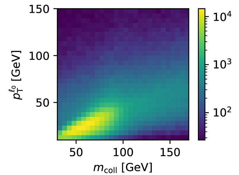
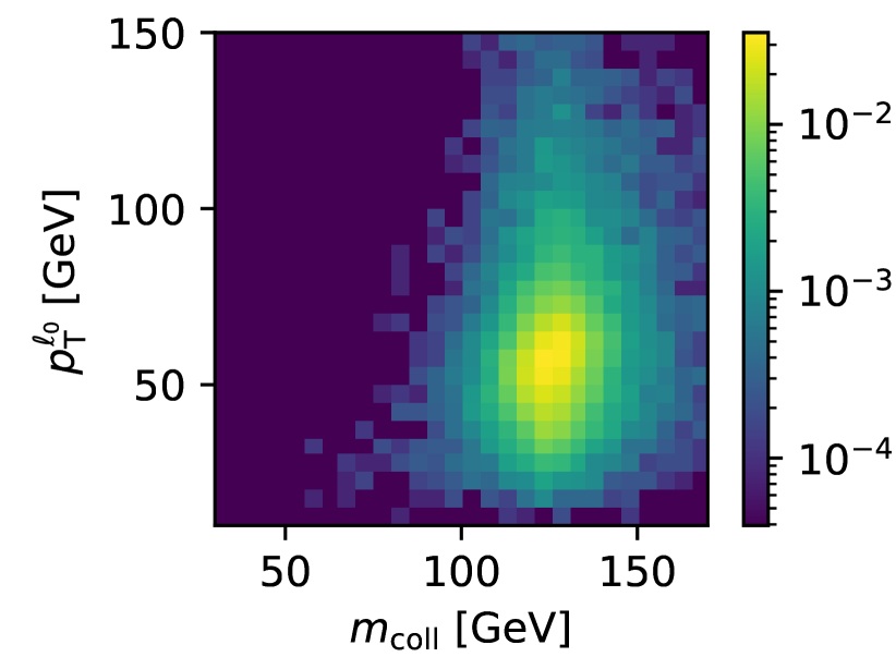
Figure 1: The $e/\mu$ background template matrix $T$ (top) and the Higgs LFV signal template matrix $S$ (bottom). The $x$, $y$ and $z$ axes are the collinear mass, leading lepton $p_{\text{T}}$ and number of entries per bin respectively ($S$ is normalized).

Other background and signals considered are flat $T$ background distributions (with either 100 or $10^{4}$ entries per bin), and rectangle and 2D Gaussian signals $S$ templates.

Given a background template $T$, which represents the underlying symmetric distribution, and a signal template $S$, which can be injected with different levels of signal-strength, the procedure to generate the samples used to qualify the different tests is as follows. From $T$ we Poisson draw $N$ pairs of $(A,B)$ background-only measurements which are symmetric up to statistical fluctuations. The background + signal measurements $B^{s}$ are obtained by injecting some signal into the $B$ samples. We inject the signal with a signal-strength $\mu_{\mathrm{inj}}$, determined such that a $q_{0}$ test for discovery ($q_{0}^{L1}$ or $q_{0}^{L2}$) outputs a given significance $Z_{\mathrm{inj}}$ when testing ${B^{s}=B+\mu_{\mathrm{inj}}S}$ against $B$:

$$\sqrt{q_{0}}(B+\mu_{\mathrm{inj}}S,B,S)=Z_{\mathrm{inj}}\,.$$ (11)

Since $S$ is normalized, $\mu_{\mathrm{inj}}$ is the number of signal events added to the $B$ sample.

Explicitly, for the $q_{0}^{L1}$ and $q_{0}^{L2}$ cases, it is found by solving Equations 12 and 13, respectively:

$$2\left(-\mu_{\mathrm{inj1}}+\sum\limits_{i=1}^{M}\left[(B_{i}+\mu_{\mathrm{inj1}}S_{i})\ln\left(1+\mu_{\mathrm{inj1}}\frac{S_{i}}{B_{i}}\right)\right]\right)=Z_{\mathrm{inj1}}^{2}$$ (12)

$$2\sum\limits_{i=1}^{M}\left[(B_{i}+\mu_{\mathrm{inj2}}S_{i})\ln\left(1+\mu_{\mathrm{inj2}}\frac{S_{i}}{2B_{i}+\mu_{\mathrm{inj2}}S_{i}}\right)\right.\\ \left.-B_{i}\ln\left(1+\mu_{\mathrm{inj2}}\frac{S_{i}}{2B_{i}}\right)\right]=Z_{\mathrm{inj2}}^{2}$$ (13)

For each separate experiment considered and detailed below, the number of $A$, $B$ and ${B^{s}=B+\mu_{\mathrm{inj}}S}$ matrices we generate is $N=20000$. For the $N_{\sigma}$ and $q_{0}^{L2}$ tests, the PDFs of the symmetric case (background-only) are obtained by comparing the $B$ and $A$ pairs, and the PDFs of the asymmetric case (signal+background) by comparing the $B^{s}$ and $A$ pairs. The same is applied for the $q_{0}^{L1}$ test, when the $A$ matrices are replaced by the template $T$.

4 Results

Focusing on the Higgs LFV example, using the signal ($S$) and background ($T$) templates shown in Figure 1, we apply an injected signal-strength $\mu_{\mathrm{inj}}$ which corresponds to $5\sigma$ significance of the ideal $q_{0}^{L1}$ test. To give an impression, when applied to $T$, this corresponds to a signal fraction of 0.2%, or in a $6\times 6$ window centered around the signal of 2.8%. In Figure 2, we compare $Z$ PDFs obtained with the $q_{0}^{L1}$, $q_{0}^{L2}$ and $N_{\sigma}$ tests. As expected, the symmetric-case PDFs of all tests are consistent with standard Gaussian distributions. We observe that the background + signal (asymmetric-case) PDFs are consistent with Gaussians with variance $1\pm 0.05$ (for all examples considered), centered around the resulting average significance $Z_{\mathrm{avg}}$ of the relevant test. The $Z_{\mathrm{avg}}$ of each test can be directly estimated by using the Asimov data eilamStat ; setting $A=T$ and $B^{s}=T+\mu_{\mathrm{inj}}S$. The resulting significance with the $q_{0}^{L1}$ test is predictably $Z_{\mathrm{avg}}=5.0\approx Z_{\mathrm{inj}}$. With $Z_{\mathrm{avg}}=3.53$, $q_{0}^{L2}$ is less sensitive than $q_{0}^{L1}$ since it does not use an a priori knowledge of the background, but estimates it from the two measurements as part of the fitting procedure. Since the $N_{\sigma}$ test is averaged on all the bins, and most of them only include background contributions, the resulting average significance $Z_{\mathrm{avg}}=1.48$ is significantly lower than the separation power measured with the $q_{0}^{L2}$ test.

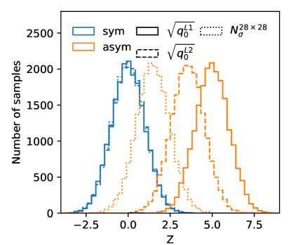
Figure 2: Significance PDFs comparing results of the $N_{\sigma}$, $q_{0}^{L1}$ and $q_{0}^{L2}$ tests for the Higgs LFV example, with injected signal strength corresponding to $5\sigma$ of $q_{0}^{L1}$.

In general, it can be much more efficient to apply the $N_{\sigma}$ test in a sub-region of the data samples. Even though the signal’s shape and location is not known in a generic test, since the calculation of $N_{\sigma}$ is fast, one could test multiple bin subsets, or develop an algorithm to optimize this selection. In Figure 3, we show $N_{\sigma}$ scores with the Asimov data, obtained when the test is performed on square windows of different sizes, centered around the location of the signal. The $N_{\sigma}$ sensitivity increases when the window encapsulates the signal region more precisely, reaching up to $Z_{\mathrm{avg,max}}=2.74$ with the $6\times 6$ bins window. Thus, for this example, the sensitivity achieved is only slightly worse than the one achieved with the $q_{0}^{L2}$ test, which exploits a full knowledge of the signal shape. The $N_{\sigma}$ results presented hereafter are for the best suited window ($6\times 6$ bins for all examples considered).

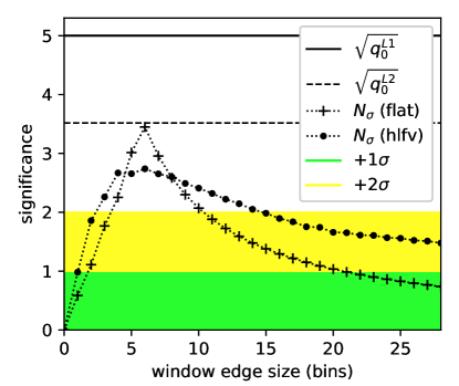
Figure 3: Significance measured from the Asimov data, with the $N_{\sigma}$ test applied to increasing window sizes, and compared to the $q_{0}^{L1}$ and $q_{0}^{L2}$ significance. Results for the Higgs LFV example and the ideal (flat) scenario are shown, with injected signal strength corresponding to $5\sigma$ of $q_{0}^{L1}$. The green and yellow bands correspond to the 1$\sigma$ and $2\sigma$ deviations from the symmetry (no signal) assumption, respectively.

In Figure 4 we show the Receiver Operating Characteristic (ROC) curves obtained from the PDFs of the different tests. The Area-Under-Curve (AUC) measured is approximately 1.0 for the $q_{0}^{L1}$ test and 0.994 for the $q_{0}^{L2}$ test. With an AUC of $=0.973$, the $N_{\sigma}$ test is only 2.6% less sensitive than the $q_{0}^{L1}$ test, and 2.0% less sensitive than the $q_{0}^{L2}$ test. Finally, in Figure 5, we show $Z_{\mathrm{avg}}$ per test (estimated from the Asimov data), for increasing injected signal strength. Using the $N_{\sigma}$ test statistic, the symmetric case (background only) can be separated from the asymmetric case at the level of $2\sigma$ if the signal that would have been measured assuming an ideal analysis ($q_{0}^{L1}$) is at the level of $3.5\sigma$. This should be compared also to the $2.5\sigma$ separation that would have been obtained in the same case using the profile likelihood ratio test statistic that uses the two samples to estimate the symmetric background and a full knowledge of the signal shape ($q_{0}^{L2}$).

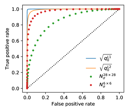
Figure 4: ROC curves comparing results of the $N_{\sigma}$, $q_{0}^{L1}$ and $q_{0}^{L2}$ tests for the Higgs LFV example, with injected signal strength corresponding to $5\sigma$ of $q_{0}^{L1}$.

For clarity, we also consider a flat background template $T$ with $10^{4}$ entries in each bin, and a flat rectangle signal template $S$ of size $6\times 6$ bins, located at the center of $T$. Since the $q_{0}^{L1}$ and $q_{0}^{L2}$ are independent of the background and signal shapes, and only depend on the injected signal strength, their symmetry- and asymmetry-case PDF will remain unchanged. The PDF associated with the $N_{\sigma}$ in the asymmetric case will change. As shown in Figures 3 and 5, in this simplified case the $N_{\sigma}$ sensitivity matches exactly the sensitivity of $q_{0}^{L2}$ test. This hints that the loss of sensitivity of the generic $N_{\sigma}$ test, compared to $q_{0}^{L2}$, is mainly due to shape variations of the background and the signal (in the optimal sub-region that is tested). But even in a realistic scenario like the Higgs LFV example, the sensitivity loss is reasonable (from $Z_{\mathrm{avg}}=3.53$ to 2.74) and the power achieved to identify regions with asymmetry, even though the $N_{\sigma}$ test is generic, is significant.

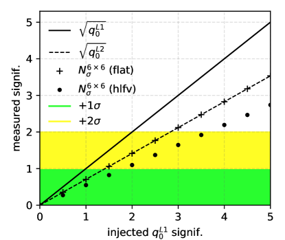
Figure 5: Significance measured from the Asimov data for increasing injected signal, comparing results of the $N_{\sigma}$, $q_{0}^{L1}$ and $q_{0}^{L2}$ tests. Results for the Higgs LFV example and the ideal (flat) scenario are shown. The green and yellow bands correspond to the 1$\sigma$ and $2\sigma$ deviations from the symmetry (no signal) assumption, respectively.

In terms of the ability to identify asymmetries, similar performance was obtained for all the other shapes of signal and background considered.

5 Identifying asymmetries with Neural Networks

Machine learning-based anomaly detection methods constructed by comparing two samples are categorized as weakly- or semi-supervised learning because both samples are mostly background and one of them will have more signal than the other. The sample with more potential signal is given a noisy label of one and the other sample is given a label of zero. A classifier trained to distinguish the two samples can then automatically identify subtle differences between the samples without explicitly setting up bins. Existing proposals construct the samples from signal region / sideband regions ano1 ; ano2 ; gensearch2 , from data versus simulation DAgnolo:2018cun ; DAgnolo:2019vbw ; dAgnolo:2021aun ; Chakravarti:2021svb , as well as other approaches Amram:2020ykb ; Nachman:2020lpy ; Andreassen:2020nkr ; Benkendorfer:2020gek ; Hallin:2021wme . We propose to extend this methodology to symmetries.

The combination of machine learning and symmetry has received significant attention. For a given symmetry, one can construct machine learning methods that are invariant or covariant (in machine learning, this is called equivariant) under the action of that symmetry. For example, recent proposals have shown how to construct Lorentz covariant neural networks symNN1 ; symNN2 ; Qiu:2022xvr . Symmetries can also be used to build a learned representation of a sample symNN3 . There have also been proposals to use machine learning methods to discover symmetries automatically in samples symNN4 ; symNN5 ; symNN6 . In the context of BSM searches, Ref. chris1 ; chris2 recently described how to use a weakly supervised-like approach to test if a given symmetry is broken by applying the transformation to the input data. Our approach also starts by positing a symmetry, but we do not apply the symmetry transformation to each data point. Instead, we have two samples which should be statistically identical in the presence of a symmetry, but which could be different when BSM is present.

In the following, we demonstrate the concept of identifying asymmetries using a weakly supervised approach. Considering the $e\mu$ symmetry example discussed above, one of the samples is the $e\mu$ sample and the other is the $\mu e$ sample. The same two-dimensional space as described earlier is used for illustration; extending to higher dimensions is technically straightforward. A deep neural network with three hidden layers and 50 nodes per layer is used for the classifier. Rectified Linear Units (ReLU) are used for all intermediate layers and the output is passed through a sigmoid function. This network is implemented using Keras keras and Tensorflow tensorflow using Adam adam for optimization. We train for 20 epochs with a batch size of 200. None of these parameters were optimized. Figure 6 shows the symmetry/asymmetry separation power of the NN as a function of the signal fraction injected to the $\mu e$ sample. The background-only band is computed via bootstrapping efron1979 . For each bootstrap, two samples are created by drawing from the $e\mu$ and $\mu e$ events with replacement. By mixing the two samples, any asymmetry is removed.

There is no unique way to quantify the NN performance. An optimal test statistic by the Neyman-Pearson Lemma neyman1933ix is monotonically related to the likelihood ratio. Ref. DAgnolo:2018cun ; DAgnolo:2019vbw ; Nachman:2021yvi ; dAgnolo:2021aun show how to modify the loss function so that the average loss approximates the (log) likelihood ratio. Here, we find that in practice, the maximum NN score using the standard binary cross entropy loss function is an effective statistic, which goes from 0.5 in the case of no signal and increases as more signal is injected. The background-only band in Figure 6 is computed via bootstrapping and where the blue line and green/yellow bands cross indicate the approximate $1\sigma/2\sigma$ exclusion. The NN is able to automatically identify the presence of BSM for signal fractions that are a few per mil, corresponding to around 5$\sigma$ significance calculated with the ideal $q_{0}^{L1}$ test. Future explorations of this idea will understand the best way to set up the training, what statistics are most effective, and how to best extend to higher dimensions.

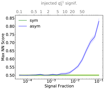
Figure 6: The maximum neural network score from training a classifier to distinguish the $e\mu$ from $\mu e$ samples with (asym) and without (sym) a BSM contribution. The green (yellow) and blue bands represent (twice) the standard deviation over 10 bootstrap samples.The separation power is shown as a function of the injected signal fraction (bottom scale) and the corresponding significance calculated with the ideal $q_{0}^{L1}$ test. Note that these results are not directly comparable to the binned DDP because it is not possible to ignore signal statistical uncertainties.

6 Discussion

With limited resources at hand and yet no conclusive indication of BSM physics found, we must try novel and complementary avenues for discovery. To overcome the limitations stemming from adapting the blind-analysis strategy, we propose developing the DDP. Similarly to D0:2000vuh ; H1:2008aak ; gensearchCDF ; gensearch1 ; gensearch3 yet without relying on MC simulations, its principal objective is to allow scanning as many regions of the observable-space as possible and direct dedicated analyses towards the ones in which the data itself exhibits deviation from some fundamental and theoretically well-established property of the SM. Relative to regions in which the data agrees well with the SM predictions, the ones that exhibit deviations are promising for further investigations into BSM physics.

We propose developing the DDP based on symmetries of the SM and demonstrate its potential sensitivity using as an example the $e/\mu$ symmetry. Symmetries allow splitting the data into two mutually exclusive samples which, under the symmetry assumption, differ only by statistical fluctuations. Thus, asymmetry observed between the two samples in any observable and at any sub-selection of these samples, is potentially interesting and should be considered for further study.

While different algorithms can be developed to identify asymmetries, even the most simple one developed, the $N_{\sigma}$ test statistic, already provides good sensitivity. It is compared to the sensitivity obtained with two likelihood-based test statistics; the first, $q_{0}^{L1}$, represents an ideal analysis in which both the signal and the symmetric contribution from the SM processes are perfectly known. The second, $q_{0}^{L2}$, represents the expected sensitivity of a traditional blind analysis search for a predefined signal that employs a symmetry-based background estimation (emmeRun1 ).

Compared to the sensitivity obtained in an ideal analysis, the separation power between the symmetric case and an asymmetry at the level of 5$\sigma$ is less than 3% lower in terms of the area under the ROC curve, and a separation at the level of $2\sigma$ is achieved for $3.5\sigma$ signal injected. Compared to a traditional symmetry-based analysis, the separation power between the symmetric case and an asymmetry at the level of 3.5$\sigma$ is less than 2% lower in terms of the area under the ROC curve, and a separation at the level of $2\sigma$ achieved using the $N_{\sigma}$ test is only slightly degraded relative to the $2.5\sigma$ obtained with the $q_{0}^{L2}$ test. The results quoted are when applying the $N_{\sigma}$ test in the best suited window for the examples considered. The ability to find this optimal window demonstrates the strength of the DDP. Since the test is rapid, a large number of n-dimensional histograms and windows within can be tested efficiently. This could permit scanning the data systematically in search for asymmetries.

We have shown that weakly-supervised NNs can also be used to identify asymmetries between two samples. This paves the way towards NN based DDP.

We emphasize that traditional blind-analyses are expected to be the most sensitive ones for any predefined signal. Nonetheless, it is impossible to conduct a dedicated search in any possible final state and at any possible event selection. Moreover, not all potential signals can be thought of. Thus, the DDP could significantly expand our discovery reach.

Data Availability Statement

The data that support the findings of this study are available from the corresponding author, MB, upon reasonable request.

References

- (1) ATLAS Collaboration, JINST 3, S08003 (2008). DOI 10.1088/1748-0221/3/08/S08003
- (2) CMS Collaboration, JINST 3, S08004 (2008). DOI 10.1088/1748-0221/3/08/S08004
- (3) B. Abbott, et al., Phys. Rev. D 62, 092004 (2000). DOI 10.1103/PhysRevD.62.092004
- (4) F.D. Aaron, et al., Phys. Lett. B 674, 257 (2009). DOI 10.1016/j.physletb.2009.03.034
- (5) CDF Collaboration, Phys. Rev. D 79, 011101 (2009). DOI 10.1103/PhysRevD.79.011101
- (6) ATLAS Collaboration, Eur. Phys. J. C 79(2), 120 (2019). DOI 10.1140/epjc/s10052-019-6540-y
- (7) ATLAS Collaboration, Phys. Rev. Lett. 125(13), 131801 (2020). DOI 10.1103/PhysRevLett.125.131801
- (8) CMS Collaboration, Eur. Phys. J. C 81(7), 629 (2021). DOI 10.1140/epjc/s10052-021-09236-z
- (9) N. Craig, P. Draper, K. Kong, Y. Ng, D. Whiteson, Acta Phys. Polon. B 50, 837 (2019). DOI 10.5506/APhysPolB.50.837
- (10) J.H. Kim, K. Kong, B. Nachman, D. Whiteson, JHEP 04, 030 (2020). DOI 10.1007/JHEP04(2020)030
- (11) S. Volkovich, F. De Vito Halevy, S. Bressler, Eur. Phys. J. C 82(3), 265 (2022). DOI 10.1140/epjc/s10052-022-10215-1
- (12) S. Bressler, A. Dery, A. Efrati, Phys. Rev. D 90(1), 015025 (2014). DOI 10.1103/PhysRevD.90.015025
- (13) C.G. Lester, B.H. Brunt, JHEP 03, 149 (2017). DOI 10.1007/JHEP03(2017)149. [Erratum: JHEP 08, 069 (2017), Erratum: JHEP 06, 014 (2019)]
- (14) ATLAS Collaboration, Eur. Phys. J. C 77(2), 70 (2017). DOI 10.1140/epjc/s10052-017-4624-0
- (15) ATLAS Collaboration. arXiv:2112.08090 (2021)
- (16) LHCb Collaboration, Nature Phys. 18(3), 277 (2022). DOI 10.1038/s41567-021-01478-8
- (17) E. Gross, O. Vitells, Eur. Phys. J. C 70, 525 (2010). DOI 10.1140/epjc/s10052-010-1470-8
- (18) N.V. Smirnov, Bull. Math. Univ. Moscou 2(2), 3 (1939)
- (19) Student, Biometrika pp. 1–25 (1908)
- (20) J.H. Collins, K. Howe, B. Nachman, Phys. Rev. Lett. 121(24), 241803 (2018). DOI 10.1103/PhysRevLett.121.241803
- (21) J.H. Collins, K. Howe, B. Nachman, Phys. Rev. D 99(1), 014038 (2019). DOI 10.1103/PhysRevD.99.014038
- (22) E.M. Metodiev, B. Nachman, J. Thaler, JHEP 10, 174 (2017). DOI 10.1007/JHEP10(2017)174
- (23) R.T. D’Agnolo, A. Wulzer, Phys. Rev. D 99(1), 015014 (2019). DOI 10.1103/PhysRevD.99.015014
- (24) R.T. D’Agnolo, G. Grosso, M. Pierini, A. Wulzer, M. Zanetti, Eur. Phys. J. C 81(1), 89 (2021). DOI 10.1140/epjc/s10052-021-08853-y
- (25) O. Amram, C.M. Suarez, JHEP 01, 153 (2021). DOI 10.1007/JHEP01(2021)153
- (26) B. Nachman, D. Shih, Phys. Rev. D 101, 075042 (2020). DOI 10.1103/PhysRevD.101.075042
- (27) A. Andreassen, B. Nachman, D. Shih, Phys. Rev. D 101(9), 095004 (2020). DOI 10.1103/PhysRevD.101.095004
- (28) K. Benkendorfer, L.L. Pottier, B. Nachman, Phys. Rev. D 104(3), 035003 (2021). DOI 10.1103/PhysRevD.104.035003
- (29) A. Hallin, J. Isaacson, G. Kasieczka, C. Krause, B. Nachman, T. Quadfasel, M. Schlaffer, D. Shih, M. Sommerhalder. arXiv:2109.00546 (2021)
- (30) R.T. d’Agnolo, G. Grosso, M. Pierini, A. Wulzer, M. Zanetti. arXiv:2111.13633 (2021)
- (31) B. Nachman. arXiv:2010.14554 (2020)
- (32) G. Karagiorgi, G. Kasieczka, S. Kravitz, B. Nachman, D. Shih. arXiv:2112.03769 (2021)
- (33) M. Feickert and B. Nachman. arXiv:2102.02770 (2021)
- (34) G. Kasieczka, et al., Rept. Prog. Phys. 84(12), 124201 (2021). DOI 10.1088/1361-6633/ac36b9
- (35) T. Aarrestad, et al., SciPost Phys. 12, 043 (2022). DOI 10.21468/SciPostPhys.12.1.043
- (36) J. Neyman, E.S. Pearson, Phil. Trans. R. Soc. Lond. A 231, 289 (1933)
- (37) G. Cowan, K. Cranmer, E. Gross, O. Vitells, Eur. Phys. J. C 71, 1554 (2011). DOI 10.1140/epjc/s10052-011-1554-0. [Erratum: Eur.Phys.J.C 73, 2501 (2013)]
- (38) J. Alwall, R. Frederix, S. Frixione, V. Hirschi, F. Maltoni, O. Mattelaer, H.S. Shao, T. Stelzer, P. Torrielli, M. Zaro, JHEP 07, 079 (2014). DOI 10.1007/JHEP07(2014)079
- (39) T. Sjöstrand, S. Ask, J.R. Christiansen, R. Corke, N. Desai, P. Ilten, S. Mrenna, S. Prestel, C.O. Rasmussen, P.Z. Skands, Comput. Phys. Commun. 191, 159 (2015). DOI 10.1016/j.cpc.2015.01.024
- (40) DELPHES 3 Collaboration, JHEP 02, 057 (2014). DOI 10.1007/JHEP02(2014)057
- (41) P. Chakravarti, M. Kuusela, J. Lei, L. Wasserman. arXiv:2102.07679 (2021)
- (42) A. Bogatskiy, B. Anderson, J.T. Offermann, M. Roussi, D.W. Miller, R. Kondor. arXiv:2006.04780 (2020)
- (43) S. Gong, Q. Meng, J. Zhang, H. Qu, C. Li, S. Qian, W. Du, Z.M. Ma, T.Y. Liu. arXiv:2201.08187 (2022)
- (44) S. Qiu, S. Han, X. Ju, B. Nachman, H. Wang. arXiv:2203.05687 (2022)
- (45) B.M. Dillon, G. Kasieczka, H. Olischlager, T. Plehn, P. Sorrenson, L. Vogel. arXiv:2108.04253 (2021)
- (46) G. Barenboim, J. Hirn, V. Sanz, SciPost Phys. 11, 014 (2021). DOI 10.21468/SciPostPhys.11.1.014
- (47) K. Desai, B. Nachman, J. Thaler. arXiv:2112.05722 (2021)
- (48) S. Krippendorf, M. Syvaeri. arXiv:2003.13679 (2020)
- (49) R. Tombs, C.G. Lester. arXiv:2111.05442 (2021)
- (50) C.G. Lester, R. Tombs. arXiv:2111.00616 (2021)
- (51) F. Chollet. https://github.com/fchollet/keras (2017)
- (52) M. Abadi, P. Barham, J. Chen, Z. Chen, A. Davis, J. Dean, M. Devin, S. Ghemawat, G. Irving, M. Isard, et al., in OSDI, vol. 16 (2016), vol. 16, pp. 265–283
- (53) D. Kingma, J. Ba. arXiv:1412.6980 (2014)
- (54) B. Efron, Ann. Statist. 7(1), 1 (1979). DOI 10.1214/aos/1176344552
- (55) B. Nachman, J. Thaler, Phys. Rev. D 103(11), 116013 (2021). DOI 10.1103/PhysRevD.103.116013