Approaching Massive MIMO Performance with Reconfigurable Intelligent Surfaces:
We Do Not Need Many Antennas

Abstract

This paper considers an antenna structure where a (non-large) array of radiating elements is placed at short distance in front of a reconfigurable intelligent surface (RIS). This structure is analyzed as a possible emulator of a traditional MIMO antenna with a large number of active antenna elements and RF chains. Focusing on both the cases of active and passive RIS, we tackle the issues of channel estimation, downlink signal processing, power control, and RIS configuration optimization. With regard to the last point, an optimization problem is formulated and solved, both for the cases of active and passive RIS, aimed at minimizing the channel signatures cross-correlations and thereby reducing the interference. Downlink spectral efficiency (SE) formulas are also derived by using the popular hardening lower-bound. Numerical results, represented with reference to max-fairness power control, show that the proposed structure is capable of outperforming conventional non-RIS aided MIMO systems even when the MIMO system has a considerably larger number of antennas and RF chains. The proposed antenna structure is thus shown to be able to approach massive MIMO performance levels in a cost-effective way with reduced hardware resources.

I Introduction

The increasing demand for ubiquitous connectivity along with a high quality of service is driving a rapid technological (r)evolution of the mobile wireless systems. Massive multiple-input multiple-output (MIMO) is undoubtedly a key physical layer technology for the current fifth generation (5G) of mobile wireless networks [2]. By leveraging the joint coherent transmission/reception from a large number of active antenna elements, and a fully digital baseband processing at the base station (BS), massive MIMO enables an aggressive spatial multiplexing of a large number of user equipments (UEs) in the same time-frequency resource. This leads to unprecedented levels of coverage, spectral and energy efficiency. Moreover, the use of large number of antennas triggers, in most of the propagation environments, pleasant phenomena deriving from the law of the large numbers which simplify signal processing and resource allocation, thus reducing the hardware complexity and the circuit power consumption. Nevertheless, uncontrollably increasing the number of active antenna elements (hence of RF chains) to improve the data rates is an expensive and not energy-efficient solution as the total energy consumption scales linearly with the number of RF chains while the data rates grows logarithmically utmost [3].

Reconfigurable intelligent surfaces (RISs) constitute an emerging affordable solution to aid other technologies in implementing energy-efficient communications systems, and better coping with harsh propagation environments [4, 5, 6]. An RIS is a meta-surface consisting of low-cost, typically passive, tiny reflecting elements that can be properly configured on real-time to either focus the energy towards areas where coverage or additional capacity is needed, or to null the interfering energy in specific spatial points. Basically, an RIS has the ability to shape the propagation channel and create a smart radio environment [7] so as to improve the overall performance of the communication system. Technically, each RIS element introduces a configurable phase-shift to an impinging EM wave, so that the resulting reflected beam is steered towards the desired direction. Beamforming is therefore carried out by the environment in addition to the active radiative system where the impinging wave is generated. While initially available RIS technology enabled the tuning of the phase-shift only of the reflected impinging waves, recently new types of RISs, nicknamed active RIS, have been introduced, with the capability of controlling both the amplitude and the phase of the reflected waves [9, 8].

In this paper we investigate an architecture where the RIS is placed at short distance (i.e., few wavelengths) from a not-large array of active antennas, as a proxy of a conventional massive MIMO antennas with large number of elements and RF-chains. The goal of the paper is to show indeed that thanks to the use of the RIS the multiplexing capabilities and performance of conventional MIMO systems can be approached with a much smaller number of active antennas and RF chains.

I-A Related Works

A typical RIS-aided massive MIMO system consists of a BS equipped with several antennas simultaneously serving multiple UEs over a composite channel, which is composed by a direct link, from the BS to each UE, if available, and an indirect link, from the BS to the UEs through the RIS. A detailed characterization of the favourable propagation, channel hardening, and rank deficiency of the RIS-aided massive MIMO composite channel assuming Rayleigh fading is provided in [10].

Most of existing works focused on the joint optimization of the BS precoding vectors and the RIS phase-shifts, and propose effective channel estimation techniques to properly support this joint beamforming [5, 6, 7, 11].

Recently, [12] proposed a two-timescale beamforming optimization to maximize the average sum-rate of an RIS-aided multi-user communication system under the assumption of correlated Rician fading channels. Specifically, the RIS phase shifts are firstly optimized based on the statistical CSI, while the BS precoding vectors are then designed upon the use of the instantaneous CSI, and the optimized RIS phase shifts. Importantly, this solution also leads to a significant saving in terms of training overhead and RIS configuration complexity.

Similarly, [13, 14] investigates the ergodic uplink rate of an RIS-aided massive MIMO system with direct links, assuming maximum-ratio combining (MRC) and zero-forcing detector, respectively, with a low-overhead statistical CSI-based design for the RIS passive beamforming. Along this line, [15] proposes three architectures in which either a short-term RIS reconfiguration based on instantaneous CSI or a long-term RIS reconfiguration based on statistical CSI is considered. Bayesian channel estimators using a structured pilot assignment with a low training overhead are derived. These estimates are then employed in a novel receive combining scheme following the minimum mean-squared error (MMSE) principle. Interestingly, this study gives an answer to the question whether channel estimation is necessary to properly select the RIS phase-shifts: if targeting the performance of the most unfortunate UEs, and there are multiple specular channel components, a long-term RIS configuration is advantageous thus channel estimation is not needed for RIS configuration. For all other cases, a short-term RIS configuration either with a single-stage or two-stage channel estimation is preferable.

The work [16] presents a channel estimation scheme that capitalizes on the statistical characterization of the locations of the UEs for relaxing the need of frequently reconfiguring the RIS phase-shifts. Compared to other works, this approach does require the estimation of neither instantaneous nor statistical CSI for RIS optimization. While, [17] studies the ergodic SE maximization problem where only historically collected channel samples are available. In [18] a method to estimate the path gain and the angles of arrival is implemented by using limited RIS RF chains and pilots, assuming that some RIS elements are active. The work [19] presents two channel estimation methods that rely on a parallel factor tensor modeling of the received signals. Both methods enable to separate the estimates of the BS-to-RIS channels from the RIS-to-UE channels. On/off RIS element patterns are considered in [20, 21] to employ estimation techniques that exploit the induced channel sparsity. A three-stage channel estimation method based on RIS on/off switching patterns is devised in [22], and leverages the spatial channel correlations. Finally, [23] proposes an iterative least squares (LS) estimation algorithm to obtain multiple channel measurements for the estimates, corresponding to different pre-determined configurations of the RIS phase-shifts.

Active RIS, capable of introducing a tunable amplification factor to reflected waves, are introduced in [9, 8], where it is discussed how passive RISs are effective under harsh propagation conditions, in scenarios where the direct paths are heavily obstructed [5], otherwise the capacity gains (of a passive RIS) c ompared to a conventional massive MIMO system become negligible [9, 8]. Moreover, accurate channel state information (CSI) acquisition relying on uplink pilots is challenging due to the passive nature of the RIS components, and the amount of pilot-symbols needed.

I-B Summary of paper contribution

In this paper, we consider an antenna structure where a (non-large) array of radiating elements is placed at short distance in front of an RIS. Although this structure has been considered elsewhere (e.g., [24]), to the best of our knowkedge this is the first paper that provides a thorough design and analysis about the use of such structure at sub-6 GHz frequencies, addressing challenging issues such as channel estimation (a critical problem in RIS-aided wireless communications), optimal RIS configuration, derivation of spectral efficiency bounds, and extension to the case of active RIS. In particular, the contribution of this paper may be summarized as follows.

With reference to a single-cell system, we develop the signal model for both the cases of active and passive RIS, and provide theoretical considerations on the achievement of favourable propagation and channel hardening for the proposed antenna structure. Next, in order to cope with the critical problem of channel estimation, we introduce reduced-dimensionality linear minimum mean square error channel estimators. The proposed estimation scheme neglects the projection of the channel vectors onto the noise-dominated subspace. Next, we propose RIS configuration optimization algorithms, for both active and passive RISs, aimed at minimizing mutual correlation among the channel coefficient vectors of different users. Moreover, we derive closed form lower bounds to the achievable spectral efficiency, explicitly taking into account the channel estimation error, using the hardening lower-bound technique. Then, we perform extensive numerical simulations aimed at gaining insight into the performance of the proposed antenna architecture, also in comparison with a traditional massive MIMO deployment with active antennas and fully digital beamforming. Overall, the paper will show that the suggested architecture can emulate the performance of traditional massive MIMO arrays with much lower hardware complexity, i.e. with a significantly smaller numer of active antennas and RF chains.

I-C Paper organization

The paper is organized as follows. Next section contains the description of the considered antenna architecture and of the system model. Section III is concerned with the issue of channel estimation, whereas Section IV contains the derivation of the downlink signal model and of the upper and lower bounds for the spectral efficiency. Section V is devoted to system optimization; in particular, this section addresses configuration of the RIS (for both the active and passive case), and power allocation, including the power split between the active antenna array and the RIS (for the case of active RIS). Sections VI contains the discussion of the numerical results, while, finally, concluding remarks are reported in Section VII.

I-D Notation

We use non-bold letters for scalars, $a$ and $A$, lowercase boldface letters, $\mathbf{a}$, for vectors and uppercase lowercase letters, $\mathbf{A}$, for matrices. The transpose, the inverse and the conjugate transpose of a matrix $\mathbf{A}$ are denoted by $\mathbf{A}^{{T}}$, $\mathbf{A}^{-1}$ and $\mathbf{A}^{H}$, respectively. The trace and the main diagonal of the matrix $\mathbf{A}$ are denoted as tr$\left(\mathbf{A}\right)$ and diag$\left(\mathbf{A}\right)$, respectively. The diagonal matrix obtained by the scalars $a_{1},\ldots,a_{N}$ is denoted by diag$(a_{1},\ldots,a_{N})$. The $N$-dimensional identity matrix is denoted as $\mathbf{I}_{N}$, the $(N\times M)$-dimensional matrix with all zero entries is denoted as $\mathbf{0}_{N\times M}$ and $\mathbf{1}_{N\times M}$ denotes a $(N\times M)$-dimensional matrix with unit entries. The vectorization operator is denoted by vec$(\cdot)$ and the Kronecker product is denoted by $\otimes$. Given the matrices $\mathbf{A}$ and $\mathbf{B}$, with proper dimensions, the horizontal concatenation is denoted by $\left[\mathbf{A},\mathbf{B}\right]$. The $(m,\ell$)-th entry and the $\ell$-th column of the matrix $\mathbf{A}$ are denoted as $\left[\mathbf{A}\right]_{(m,\ell)}$ and $\left[\mathbf{A}\right]_{(:,\ell)}$, respectively. The block-diagonal matrix obtained from matrices $\mathbf{A}_{1},\ldots,\mathbf{A}_{N}$ is denoted by $\mathsf{blkdiag}\left(\mathbf{A}_{1},\ldots,\mathbf{A}_{N}\right)$. The statistical expectation and variance operators are denoted as $\mathsf{E}\!\left\{{\cdot}\right\}$ and $\text{var}\{\cdot\}$ respectively; $\mathcal{CN}\left(\mu,\sigma^{2}\right)$ denotes a complex circularly symmetric Gaussian random variable with mean $\mu$ and variance $\sigma^{2}$.

Figure 1: (a) A possible configuration of the considered RIS-aided antenna structure in 3D space. A small planar array with $N_{A}$ active antennas is mounted at close distance from an RIS with $N_{R}$ elements. The relative positioning of the active array and of the RIS is such that no obstruction is created between the RIS and the UEs on the ground. (b) Proposed arrangement of active array and RIS for a 2D layout, in case of (top) omnidirectional and (bottom) directional antennas radiating in the angular sector $[-\pi/2,\pi/2]$ and $[-\pi/4,\pi/4]$, respectively.

II System model

Consider a single-cell system where a BS is equipped with an RIS-aided antenna array, and serves $K$ single-antenna UEs, as depicted in Fig. 1(a). We denote by $N_{A}$ the elements of the active antenna array, and by $N_{R}>N_{A}$ the number of configurable reflective elements of the RIS. The uplink channel between the $k$-th UE and the RIS is represented by the $N_{R}$-dimensional vector ${\mathbf{h}}_{k}$, while the matrix-valued channel from the RIS to the receive antenna array is represented through the $(N_{A}\!\times\!N_{R})$-dimensional matrix $\mathbf{H}$.

We consider both the cases of passive and reflective active RISs. In the former, each element of the RIS solely introduces a tunable phase offset on the impinging waves, and does not alter its amplitude; whereas in the latter, we assume that each element of the RIS performs an amplify-and-reflect operation, as described in [8], so that the reflected wave is modified both in its amplitude and phase. Such a reflective active RIS is obtained by exclusively integrating an active reflection-type amplifier in each RIS element, and differs from an active RIS equipped with an RF chain per active element. The latter needs higher hardware complexity to support its baseband processing capability, and operates similarly to a decode-and-forward relay [28, 29, 30]. Conversely an active reflection-type amplifier can be implemented by using low-cost, low-power-consumption components such as cross-coupled structures of transistors [31], multi-layer integrated circuits [32], and current-inverting converters [33].

Regardless of the RIS typology, the effect of the RIS is modeled as a diagonal $(N_{R}\times N_{R})$-dimensional matrix, denoted by $\mathbf{P}$. The diagonal entries of $\mathbf{P}$ are constrained to have unit modulus in case of passive RIS, whereas they have a tunable magnitude in case of active RISs. According to the description above, the composite uplink channel from the $k$-th UE to the active array is the $N_{A}$-dimensional vector

$$\bar{\mathbf{h}}_{k}=\mathbf{H}\mathbf{P}\mathbf{h}_{k},$$ (1)

with $\mathbf{h}_{k}$ the $N_{R}$-dimensional vector describing the uplink channel from the $k$-th UE to the RIS.

II-A Channel Model

Under the rich-scattering assumption, usually verified at sub-6 GHz frequencies, the channel vector $\mathbf{h}_{k}$ is written as $\mathbf{h}_{k}=\sqrt{\beta_{k}}\mathbf{g}_{k}$, where $\mathbf{g}_{k}$ is a complex Gaussian distributed vector with zero mean and covariance matrix $\mathbf{I}_{N_{R}}$, and $\beta_{k}$ representing the large-scale fading coefficient for the $k$-th UE.

Regarding the RIS-to-active array $(N_{A}\!\times\!N_{R})$-dimensional matrix $\mathbf{H}$, we refer here, for the sake of simplicity, to the two-dimensional schematic illustration in Fig. 1(b), where we have an active array that illuminates a large RIS placed at a short distance, that we denote by $D$; the UEs to be served are placed in the backside of the active antenna array. We make the following assumptions:

• We neglect the blockage that the active array can introduce on the electromagnetic radiation reflected by the RIS. In practical 3D scenarios, the active array can be placed laterally with respect to the RIS so as to simply avoid the blockage problem; see for instance the Fig. 1(a).

• The direct signal from the active antenna array to the mobile UEs will be neglected because it is considerably weaker than that from the RIS-reflected signal.

• Given the short distance between the RIS and the active antenna array, the channel $\mathbf{H}$ is modeled as a deterministic quantity.

• We neglect the mutual coupling between the elements of the active array and between the elements of the RIS. This is an assumption that is usually verified provided that the element spacing at the active array and at the RIS, i.e. $d_{A}$ and $d_{R}$, respectively, does not fall below the typical $\lambda/2$ value [34], with $\lambda$ being the wavelength corresponding to the radiated frequency.

• We assume that each element of the RIS is in the far field of each element of the active antenna array. However, the whole RIS is not required to be in the far field of the whole active antenna array.

With regard to assumption v), the far field condition among the generic $i$-th transmit antenna and $j$-th RIS element is $d_{i,j}>2\max\{\Delta_{A}^{2},\Delta_{R}^{2}\}/\lambda$ and $d_{i,j}\gg\max\{\Delta_{A},\Delta_{R},\lambda\}$, with $\Delta_{A}$ and $\Delta_{R}$ the size of the active antenna and RIS element, respectively [35]. The fulfilment of the far-field condition among the whole RIS and the whole active array would have instead required that the validity of the previous conditions with $d_{i,j}$, $\Delta_{A}$ and $\Delta_{R}$ replaced by $D$, $N_{A}d_{A}$ and $N_{R}d_{R}$, respectively. The absence of the far field assumption between the whole active array and the RIS, although making the matrix $\mathbf{H}$ modelling somewhat more involved, is crucial in order to have a matrix channel with rank $>1$, that will permit communicating along many signal space directions.

Based on the above assumptions, and according to standard electromagnetic radiation theory, the $(i,j)$-th entry of $\mathbf{H}$, say $\mathbf{H}(i,j)$, representing the uplink channel coefficient from the $j$-th element of the RIS to the $i$-th active antenna, can be written as[24]:

$$\mathbf{H}(i,j)=\displaystyle\sqrt{\rho G_{A}(\theta_{i,j})G_{R}(\theta_{i,j})}\frac{\lambda}{4\pi d_{i,j}}e^{-\mathrm{i}2\pi d_{i,j}/\lambda}\;,$$ (2)

where $G_{A}(\theta_{i,j})$ and $G_{R}(\theta_{i,j})$ represent the $i$-th active antenna and the $j$-th RIS element gains corresponding to the look angle $\theta_{i,j}$ (see Fig. 1(b)), while $\rho\leq 1$ is a real-valued term modeling the RIS efficiency in reflecting the impinging waves.

II-B Active antenna array deployment

As we will see in the sequel of the paper, the configuration of the active antenna array affects the achievable system performance. In particular, one possible choice is to assume that the active array is made of antennas radiating towards the RIS in the angular sector $[-\pi/2,\pi/2]$ (see upper part of Fig. 1(b)); in this case the gain $G_{A}(\cdot)$ in (2) can be taken equal to 3 dB. One other possibility is to assume that the antennas of the active array radiate in a narrower angular sector (see lower part of Fig. 1(b)); denoting by $\alpha$ the width of such angular sector, the gain $G_{A}(\theta)$ is taken equal to

$$G_{A}(\theta)=\left\{\begin{array}[]{ll}\displaystyle\log_{10}\left(\frac{2\pi}{\alpha}\right),&\textit{if }\theta\in[-\alpha/2,\alpha/2],\\ 0,&\text{otherwise}\end{array}\right.$$ (3)

In this latter situation, elements of the active antenna array are to be spaced at a distance $d_{A}>\lambda/2$ in order to ensure that each RIS element is illuminated by the main beam of at least one element of the active antenna array. Based on simple geometrical considerations, a suitable antenna spacing in this case is

$$d_{A}=\displaystyle\frac{(N_{R}-1)d_{R}-2D\tan{\alpha/2}}{N_{A}-1}\,.$$ (4)

II-C Comments

Before proceeding to the system design and analysis, some considerations are needed about the channel hardening and favourable propagation. First of all, we note that, given the $k$-th UE composite signature in (1), the case of a traditional MIMO array with $N_{R}=N_{A}$ active antennas can be obtained by letting $\mathbf{H}=\mathbf{P}=\mathbf{I}_{N_{A}}$. For such a system, as it is well known, under the assumed uncorrelated fast fading realizations across antennas, both favourable propagation and channel hardening are observed for increasing values of $N_{A}$. Favourable propagation refers to the fact that the inner product between two different channel signatures converges to zero almost surely as the number of antennas diverges, while channel hardening refers to the fact that the squared magnitudes of the composite signatures converge to a deterministic value (that is the corresponding large scale fading coefficient multiplied by the number of antennas) as the antenna array size grows large. For finite values of the number of antennas, the favourable propagation condition can be checked by verifying that

$$f_{k,j}\triangleq\text{var}\left\{\frac{\bar{\mathbf{h}}_{k}^{{H}}\bar{\mathbf{h}}_{j}}{\displaystyle\sqrt{\mathsf{E}\!\left\{{\|\bar{\mathbf{h}}_{k}\|^{2}}\right\}\mathsf{E}\!\left\{{\|\bar{\mathbf{h}}_{j}\|^{2}}\right\}}}\right\}\rightarrow 0\;,$$ (5)

for all $k\neq j$, when the number of antennas grow large, while the channel hardening condition is checked by verifying that

$$f_{k,k}\triangleq\text{var}\left\{\frac{\|\bar{\mathbf{h}}_{k}\|^{2}}{\displaystyle{\mathsf{E}\!\left\{{\|\bar{\mathbf{h}}_{k}\|^{2}}\right\}}}\right\}\rightarrow 0\;,$$ (6)

for all $k$, again in the large array limiting regime. In particular, with straightforward computations, it is easy to show that for a traditional massive MIMO system (i.e., with no RIS) with $N_{A}$ antennas, both (5) and (6) are equal to $1/N_{A}$, and are thus vanishingly small as $N_{A}\rightarrow+\infty$. For the considered RIS-aided massive MIMO system, instead, denoting by $\lambda_{1},\ldots,\lambda_{N_{A}}$ the eigenvalues of the matrix $\mathbf{P}^{{H}}\mathbf{H}^{{H}}\mathbf{H}\mathbf{P}$, using standard linear algebra techniques, it can be shown that

$$f_{k,k}=f_{k,j}=\frac{\sum_{\ell=1}^{N_{A}}\lambda_{\ell}^{2}}{\left(\sum_{\ell=1}^{N_{A}}\lambda_{\ell}\right)^{2}}$$ (7)

We have now the following result.

Lemma: For the considered RIS-aided massive MIMO system, the quantities $f_{k,k}$ and $f_{k,j}$ defined in (5) and (6), respectively, are not smaller than $1/N_{A}$.

Proof: The proof follows readily by the Cauchy-Schwartz inequality: $|\mathbf{x}^{{H}}\mathbf{y}|^{2}\leq\|\mathbf{x}\|^{2}\|\mathbf{y}\|^{2}$, letting $\mathbf{x}=[\lambda_{1},\ldots,\lambda_{N_{A}}]^{{T}}$ and $\mathbf{y}$ equal to the $N_{A}$-dimensional vector with all entries equal to 1.  

The above Lemma reveals a somewhat disappointing result: the favourable propagation and channel hardening parameters are not affected by how large the RIS is, but they just depend on the number of active antennas. It could thus appear that there is no advantage in considering the proposed antenna structure in comparison to a traditional massive MIMO antenna with $N_{A}$ active elements. A moment thought clarifies however that the Lemma just suggests that the statistical parameters ruling channel hardening and favourable propagation do not benefit from the use of an RIS. The additional degrees of freedom provided by the tunable RIS elements can be however exploited to improve performance, for instance by forcing a larger degree of orthogonality among the composite signatures in (1). The results provided in the sequel of the paper will confirm that this intuition is correct and that the proposed structure may exhibit several advantages over a traditional massive MIMO system.

III Channel Estimation

During the uplink training phase, each UE transmits a known pilot sequence. We denote by $\bm{\varphi}_{k}$ the pilot sequence used by the $k$-th UE, with length $\tau_{p}$ samples and squared norm $\tau_{p}$. Since $N_{R}>N_{A}$, estimation of the channels $\{\mathbf{h}_{1},\ldots,\mathbf{h}_{K}\}$ requires that each UE transmits its pilot $Q$ times [36], each one with a different RIS configuration, and with $Q=\lceil N_{R}/N_{A}\rceil$ to ensure that the number of observables is not smaller than the number of unknown quantities. The pilots are drawn from a set of $\tau_{p}$ orthogonal sequences and, without loss of generality, are assumed to be real. Denoting by $\eta_{k}^{(u,t)}$ the uplink transmit power of the $k$-th UE during the training phase, the data observed at the active antenna array when the RIS assumes the $q$-th configuration is analytically described by the $(N_{A}\!\times\!\tau_{p})$-dimensional matrix

$$\mathbf{Y}^{(q)}=\!\sum_{k=1}^{K}\sqrt{\eta_{k}^{(u,t)}}\mathbf{H}\mathbf{P}_{\mathsf{tr}}^{(q)}\mathbf{h}_{k}\bm{\varphi}_{k}^{{T}}\!+\!\delta\mathbf{H}\mathbf{P}_{\mathsf{tr}}^{(q)}\widetilde{\mathbf{N}}^{(q)}\!+\!\mathbf{N}^{(q)},$$ (8)

where $\mathbf{P}_{\mathsf{tr}}^{(q)}$ is the $q$-th training configuration of the RIS, $\mathbf{N}^{(q)}$ is additive i.i.d. complex Gaussian static noise at the active antenna array. Moreover, the term $\delta\mathbf{H}\mathbf{P}_{\mathsf{tr}}^{(q)}\widetilde{\mathbf{N}}^{(q)}$ represents a dynamic noise contribution occurring in the case of active RIS, with the entries of $\widetilde{\mathbf{N}}^{(q)}$ being i.i.d. complex Gaussian RVs, and $\delta$ being a binary coefficient used to distinguish the case of active RIS ($\delta=1$) from the case of passive RIS ($\delta=0$). In order to estimate the $k$-th UE channel $\mathbf{h}_{k}$, the data $\mathbf{Y}^{(q)}$ is projected along the $k$-th UE pilot sequence, leading to the $N_{A}$-dimensional vector $\mathbf{y}_{k,q}=\mathbf{Y}^{(q)}\bm{\varphi}_{k}$, given by

$$\mathbf{y}_{k,q}=\tau_{p}\sqrt{\eta_{k}^{(u,t)}}\bar{\mathbf{h}}^{(q)}_{k}\!+\!\sum_{j\neq k}^{K}\rho_{j,k}\sqrt{\eta_{j}^{(u,t)}}\bar{\mathbf{h}}^{(q)}_{j}\!+\!\delta\widetilde{\mathbf{n}}_{k,q}\!+\!\mathbf{n}_{k,q},$$ (9)

where $\bar{\mathbf{h}}^{(q)}_{k}=\mathbf{H}\mathbf{P}_{\mathsf{tr}}^{(q)}\mathbf{h}_{k}$ is the composite uplink channel of UE $k$ observed at the $q$-th epoch, $\rho_{j,k}=\bm{\varphi}_{j}^{{T}}\bm{\varphi}_{k}$, and

$$\!\!\mathbf{n}_{k,q}\! =\!\mathbf{N}^{(q)}\bm{\varphi}_{k}\!\sim\!{\cal CN}(0,\tau_{p}\sigma_{A}^{2}\mathbf{I}_{N_{A}}),$$ (10)

$$\!\!\widetilde{\mathbf{n}}_{k,q}\! =\!\mathbf{H}\mathbf{P}_{\mathsf{tr}}^{(q)}\widetilde{\mathbf{N}}^{(q)}\bm{\varphi}_{k}\!\sim\!{\cal CN}(0,\tau_{p}\sigma_{R}^{2}\mathbf{H}\mathbf{P}_{\mathsf{tr}}^{(q)}(\mathbf{P}_{\mathsf{tr}}^{(q)})^{{H}}\mathbf{H}^{{H}}).$$ (11)

For each UE, the pilot signals observed during the $Q$ epochs are stacked in a collective $(QN_{A})$-dimensional vector as

$${\mathbf{y}}_{k}=\left[\mathbf{y}_{k,1}^{{T}},\;\ldots,\;\mathbf{y}_{k,Q}^{{T}}\right]^{{T}}.$$

Hence, $\mathbf{y}_{k}$ can be written as

$${\mathbf{y}}_{k}\!=\!\tau_{p}\sqrt{\eta_{k}^{(u,t)}}\widetilde{\mathbf{H}}_{\mathsf{tr}}\mathbf{h}_{k}\!+\!\sum_{j\neq k}^{K}\rho_{j,k}\sqrt{\eta_{j}^{(u,t)}}\widetilde{\mathbf{H}}_{\mathsf{tr}}\mathbf{h}_{j}\!+\!\delta\widetilde{\mathbf{n}}_{k}\!+\!\mathbf{n}_{k},$$ (12)

where $\widetilde{\mathbf{n}}_{k}\!=\!\left[\widetilde{\mathbf{n}}_{k,1}^{{T}},\ldots,\widetilde{\mathbf{n}}_{k,Q}^{{T}}\right]^{{T}}$, ${\mathbf{n}}_{k}\!=\!\left[\mathbf{n}_{k,1}^{{T}},\ldots,\mathbf{n}_{k,Q}^{{T}}\right]^{{T}}$, and $\widetilde{\mathbf{H}}_{\mathsf{tr}}$ is a $QN_{A}\!\times\!N_{R}$ matrix defined as

$$\widetilde{\mathbf{H}}_{\mathsf{tr}}=\left[\left(\mathbf{H}\mathbf{P}_{\mathsf{tr}}^{(1)}\right)^{{T}},\ldots,\left(\mathbf{H}\mathbf{P}_{\mathsf{tr}}^{(Q)}\right)^{{T}}\right]^{{T}}.$$ (13)

Now, given (12), it is seen that there is a linear relationship between the channel vector $\mathbf{h}_{k}$ to be estimated, and thus standard signal processing techniques could be applied to perform channel estimation. However, it can be easily realized that the matrix $\widetilde{\mathbf{H}}_{\mathsf{tr}}$, although being full-rank, is such that its eigenvalues are fastly decreasing. As a result, the channel vector $\mathbf{h}_{k}$ which in principle lies in an $N_{R}$-dimensional space, has much of his energy confined into a subspace described by the eigenvectors associated to the largest eigenvalues of the matrix $\widetilde{\mathbf{H}}_{\mathsf{tr}}$. It is thus convenient to directly estimate the projection of the channel onto such subspace, where a satisfactory signal-to-noise ratio is expected, rather then polluting the estimate with estimates of the low-energy components of the projected channel vectors. Accordingly, consider the truncated SVD of the matrix $\widetilde{\mathbf{H}}_{\mathsf{tr}}$, obtained by retaining its $S$ largest singular values, with $0\!<\!S\!<\!\text{rank}(\widetilde{\mathbf{H}}_{\mathsf{tr}})$, that is consider the approximation

$$\widetilde{\mathbf{H}}_{\mathsf{tr}}=\mathbf{U}\bm{\Lambda}\mathbf{V}^{{H}}\approx\widetilde{\mathbf{U}}\widetilde{\bm{\Lambda}}\widetilde{\mathbf{V}}^{{H}},$$ (14)

where $\mathbf{U}$ is $QN_{A}\!\times\!QN_{A}$ and unitary matrix, $\mathbf{V}$ is $N_{R}\!\times\!N_{R}$ and unitary matrix, and $\bm{\Lambda}$ is $QN_{A}\!\times\!N_{R}$ and diagonal matrix with non-negative real entries. This triplet results from the full SVD. While, $\widetilde{\mathbf{U}}$ is $QN_{A}\!\times\!S$ and unitary matrix, $\widetilde{\mathbf{V}}^{{H}}$ is $S\!\times\!N_{R}$ and unitary matrix, and $\bm{\Lambda}$ is $S\!\times\!S$ and diagonal matrix with positive real entries representing the most significant singular values of $\widetilde{\mathbf{H}}_{\mathsf{tr}}$. Notice that the approximation in (14) is accurate if $\widetilde{\mathbf{H}}_{\mathsf{tr}}$ has $S$ dominant singular values. This is likely to occur in the considered scenario because of the structure of the channel matrix $\mathbf{H}$. We can now approximate $\mathbf{h}_{k}$ as follows

$$\mathbf{h}_{k}\approx\widetilde{\mathbf{V}}\widetilde{\mathbf{V}}^{{H}}\mathbf{h}_{k}=\widetilde{\mathbf{V}}\widetilde{\mathbf{v}}_{k},$$

where we defined $\widetilde{\mathbf{v}}_{k}\!=\!\widetilde{\mathbf{V}}^{{H}}\mathbf{h}_{k}$. By using (14), the observable in (12) can be approximated as ${\mathbf{y}}_{k}\approx\widetilde{\mathbf{y}}_{k}$, where

$$\widetilde{\mathbf{y}}_{k}\!=\!\tau_{p}\sqrt{\eta_{k}^{(u,t)}}\widetilde{\mathbf{U}}\widetilde{\bm{\Lambda}}\widetilde{\mathbf{v}}_{k}\!+\!\sum_{j\neq k}^{K}\rho_{j,k}\sqrt{\eta_{j}^{(u,t)}}\widetilde{\mathbf{U}}\widetilde{\bm{\Lambda}}\widetilde{\mathbf{v}}_{j}\!+\!\delta\widetilde{\mathbf{n}}_{k}\!+\!\mathbf{n}_{k}.$$ (15)

Given (15), and using the approximation in (14), the receiver computes the $S$-dimensional vector $\overline{\mathbf{y}}_{k}=\widetilde{\mathbf{U}}^{{H}}\widetilde{\mathbf{y}}_{k}$, given by

$$\overline{\mathbf{y}}_{k}\!=\!\tau_{p}\sqrt{\eta_{k}^{(u,t)}}\widetilde{\bm{\Lambda}}\widetilde{\mathbf{v}}_{k}\!+\!\!\sum_{j\neq k}^{K}\rho_{j,k}\sqrt{\eta_{j}^{(u,t)}}\widetilde{\bm{\Lambda}}\widetilde{\mathbf{v}}_{j}\!+\!\delta\widetilde{\mathbf{U}}^{{H}}\widetilde{\mathbf{n}}_{k}\!+\!\widetilde{\mathbf{U}}^{{H}}{\mathbf{n}}_{k}.$$ (16)

Thus, the linear minimum-mean-square error (LMMSE) estimate of $\widetilde{\mathbf{v}}_{k}$ is given by $\widehat{\widetilde{\mathbf{v}}}_{k}=\mathbf{R}_{\widetilde{\mathbf{v}}_{k}\overline{\mathbf{y}}_{k}}\mathbf{R}_{\overline{\mathbf{y}}_{k}\overline{\mathbf{y}}_{k}}^{-1}\overline{\mathbf{y}}_{k},$ with

$$\mathbf{R}_{\widetilde{\mathbf{v}}_{k}\overline{\mathbf{y}}_{k}}\! \triangleq\!\mathsf{E}\!\left\{{\widetilde{\mathbf{v}}_{k}\overline{\mathbf{y}}_{k}^{{H}}}\right\}=\tau_{p}\sqrt{\eta_{k}^{(u,t)}}\beta_{k}\widetilde{\bm{\Lambda}}^{{H}},$$ (17)

$$\mathbf{R}_{\overline{\mathbf{y}}_{k}\overline{\mathbf{y}}_{k}}\! \triangleq\mathsf{E}\!\left\{{\overline{\mathbf{y}}_{k}\overline{\mathbf{y}}_{k}^{{H}}}\right\}$$

$$=\!\!\Bigg{(}\sum_{j=1}^{K}\rho_{j,k}^{2}\eta_{j}^{(u,t)}\beta_{j}\Bigg{)}\widetilde{\bm{\Lambda}}\widetilde{\bm{\Lambda}}^{{H}}\!\!+\sigma_{A}^{2}\tau_{p}\mathbf{I}_{S}\!+\!\delta\sigma_{R}^{2}\tau_{p}\mathbf{Z},$$ (18)

where $\mathbf{Z}\!=\!\widetilde{\mathbf{U}}^{{H}}~{}\mathsf{blkdiag}\!\left(\overline{\mathbf{H}}^{(1)}_{\mathsf{tr}},\ldots,\overline{\mathbf{H}}^{(Q)}_{\mathsf{tr}}\right)\widetilde{\mathbf{U}},$ and $\overline{\mathbf{H}}^{(q)}_{\mathsf{tr}}=\mathbf{H}\mathbf{P}_{\mathsf{tr}}^{(q)}(\mathbf{P}_{\mathsf{tr}}^{(q)})^{{H}}\mathbf{H}^{{H}}$. An approximate LMMSE channel estimate of ${\mathbf{h}}_{k}$, denoted by $\widehat{\mathbf{h}}_{k}$, can be thus written as

$$\widehat{\mathbf{h}}_{k}\approx\widetilde{\mathbf{V}}\widehat{\widetilde{\mathbf{v}}}_{k}=\widetilde{\mathbf{V}}\mathbf{R}_{\widetilde{\mathbf{v}}_{k}\overline{\mathbf{y}}_{k}}\mathbf{R}_{\overline{\mathbf{y}}_{k}\overline{\mathbf{y}}_{k}}^{-1}\overline{\mathbf{y}}_{k}.$$ (19)

Due to the LMMSE properties, $\widehat{\mathbf{h}}_{k}$ is Gaussian distributed with zero mean and covariance matrix

$$\mathbf{R}_{\widehat{\mathbf{h}}_{k}\widehat{\mathbf{h}}_{k}}=\widetilde{\mathbf{V}}\mathbf{R}_{\widetilde{\mathbf{v}}_{k}\overline{\mathbf{y}}_{k}}\mathbf{R}_{\overline{\mathbf{y}}_{k}\overline{\mathbf{y}}_{k}}^{-1}\mathbf{R}_{\widetilde{\mathbf{v}}_{k}\overline{\mathbf{y}}_{k}}^{{H}}\widetilde{\mathbf{V}}^{{H}}.$$ (20)

The estimation error $\widetilde{\mathbf{h}}_{k}\!=\!\mathbf{h}_{k}\!-\!\widehat{\mathbf{h}}_{k}$ is statistically independent from the channel estimate $\widehat{\mathbf{h}}_{k}$ and is a zero-mean complex Gaussian vector with $\mathbf{R}_{\widetilde{\mathbf{h}}_{k}\widetilde{\mathbf{h}}_{k}}\!=\!\beta_{k}\mathbf{I}_{N_{R}}\!-\!\mathbf{R}_{\widehat{\mathbf{h}}_{k}\widehat{\mathbf{h}}_{k}}$ as covariance matrix. Notice that if two UEs, $k$ and $j$, are assigned the same pilot sequence at the epoch $q$ of the uplink training phase, hence $\bm{\varphi}_{k}\!=\!\bm{\varphi}_{j}$, then it holds $\mathbf{y}_{k,q}=\mathbf{y}_{j,q}$, and the channel estimates $\widehat{\mathbf{h}}_{k}$ and $\widehat{\mathbf{h}}_{j}$ will be proportional to each other as

$$\widehat{\mathbf{h}}_{k}=c_{k,j}\widehat{\mathbf{h}}_{j},\,\text{with }c_{k,j}=\frac{\beta_{k}}{\beta_{j}}\sqrt{\frac{\eta_{k}^{(u,t)}}{\eta_{j}^{(u,t)}}}.$$ (21)

IV Performance Measures

During the downlink data transmission phase, the signal received by the $k$-th UE in the $t$-th channel use (we omit the dependency on $t$ for brevity) is given by

$$r_{k}= \sqrt{\eta_{k}^{(d)}}\bar{\mathbf{h}}^{{T}}_{k}\mathbf{w}_{k}x_{k}\!+\!\sum_{j\neq k}^{K}\sqrt{\eta_{j}^{(d)}}\bar{\mathbf{h}}_{k}^{{T}}\mathbf{w}_{j}x_{j}\!+\!\delta\widetilde{z}_{k}\!+\!z_{k},$$ (22)

where $\eta_{k}^{(d)}$ is the downlink transmit power, $\mathbf{w}_{k}$ denotes the $N_{A}$-dimensional precoding vector, and $x_{k}$ is the data symbol intended for UE $k$, which is drawn from a constellation with unit average energy. The term $z_{k}\!\sim\!{\mathcal{CN}}(0,\sigma^{2}_{k})$ is additive white Gaussian noise at the UE $k$, while $\delta\widetilde{z}_{k}$ is non-zero if $\delta=1$, and denotes the noise introduced by the active RIS, with $\widetilde{z}_{k}\!=\!\mathbf{h}_{k}^{{T}}\mathbf{P}\mathbf{z}_{R}$, and $\mathbf{z}_{R}\!\sim\!\mathcal{CN}(\mathbf{0}_{N_{R}},\sigma^{2}_{R}\mathbf{I}_{N_{R}})$.

IV-A Instantaneous SINR and SE upper bound

For benchmarking purposes, we begin considering the ideal case in which perfect CSI is available both at the active array and at the UEs. Given (22), the downlink signal-to-interference-plus-noise ratio (SINR) at the $k$-th UE, under the perfect CSI assumption, is given by

$$\gamma_{k}^{(d)}\!=\!\frac{\eta_{k}^{(d)}\left|\mathbf{h}_{k}^{{T}}\mathbf{P}\mathbf{H}^{{T}}\mathbf{w}_{k}\right|^{2}}{\displaystyle\sum\nolimits_{j\neq k}^{K}\eta_{j}^{(d)}\left|\mathbf{h}_{k}^{{T}}\mathbf{P}\mathbf{H}^{{T}}\mathbf{w}_{j}\right|^{2}\!+\!\delta\left\lVert\mathbf{h}_{k}^{{T}}\mathbf{P}\right\rVert^{2}\!\sigma^{2}_{R}\!+\!\sigma^{2}_{k}}.$$ (23)

Consequently, assuming Gaussian-distributed infinite-length codewords, a SE for the $k$-th UE can be obtained by using the classical Shannon expression

$$\text{SE}_{k,\mathsf{PCSI}}^{(d)}=\xi\log_{2}\Big{(}1+\gamma_{k}^{(d)}\Big{)},\quad[\mbox{bit/s/Hz}],$$ (24)

where $\xi$ accounts for the fraction of the channel coherence interval used for the downlink data transmission.

Under the assumption of imperfect CSI, an upper bound of the downlink achievable SE, is obtained by optimistically assuming perfect knowledge of the channel estimates at the UEs, which leads to [37]

$$\text{SE}_{k,\mathsf{UB}}^{(d)}=\bar{\xi}~{}\mathsf{E}\!\left\{{\log_{2}\Big{(}1+\gamma_{k}^{(d)}\Big{)}}\right\},\quad[\mbox{bit/s/Hz}].$$ (25)

In (25) the expectation is computed over the small-scale fading quantities, and the beamforming vectors $\mathbf{w}_{1},\ldots,\mathbf{w}_{K}$ are designed upon the channel estimates.

IV-B The hardening bound

To obtain an achievable SE expression in closed-form, we derive the so-called hardening lower-bound on the capacity, as detailed in [2], according to which an achievable SE for the $k$-th UE can be obtained by assuming UEs’ knowledge of only the channel statistics, and treating all the interference and noise contributions as uncorrelated effective noise. Letting

$$r_{k} =\sqrt{\eta_{k}^{(d)}}\underbrace{\mathsf{E}\!\left\{{\bar{\mathbf{h}}_{k}^{{T}}\mathbf{w}_{k}}\right\}}_{\mathsf{DS}_{k}}x_{k}\!+\!\sqrt{\eta_{k}^{(d)}}\underbrace{\left(\bar{\mathbf{h}}_{k}^{{T}}\mathbf{w}_{k}\!-\!\mathsf{E}\!\left\{{\bar{\mathbf{h}}_{k}^{{T}}\mathbf{w}_{k}}\right\}\right)}_{\mathsf{BU}_{k}}x_{k}$$

$$\quad+\sum\limits_{j\neq k}^{K}\sqrt{\eta_{j}^{(d)}}\underbrace{\bar{\mathbf{h}}_{k}^{{T}}\mathbf{w}_{j}}_{\mathsf{UI}_{k,j}}x_{j}+\delta\widetilde{z}_{k}+z_{k},$$ (26)

and assuming power control coefficients depending only on the large-scale fading, the hardening lower-bound is given by

$$\text{SE}_{k,\mathsf{LB}}^{(d)}=\bar{\xi}\log_{2}\Big{(}1+\gamma_{k,\mathsf{LB}}^{(d)}\Big{)},$$ (27)

with $\gamma_{k,\mathsf{LB}}^{(d)}$ defined as

$$\!\frac{\eta_{k}^{(d)}\left|\mathsf{DS}_{k}\right|^{2}}{\!\eta_{k}^{(d)}\mathsf{E}\!\left\{{\left|\mathsf{BU}_{k}\right|^{2}}\right\}\!+\!\!\sum\nolimits_{j\neq k}^{K}\!\eta_{j}^{(d)}\mathsf{E}\!\left\{{\left|\mathsf{UI}_{k,j}\right|^{2}}\right\}\!+\!\delta\mathsf{E}\!\left\{{|\widetilde{z}_{k}|^{2}}\right\}\!+\!\sigma^{2}_{k}},$$ (28)

where the first term in (IV-B) represents the deterministic desired signal (DS), the second term represents the self-interference due to the unknown channel estimate (BU, which stands for beamforming gain uncertainty), the third term is the multi-user interference (UI), and, lastly, the fourth and fifth terms are uncorrelated noise. Assuming channel independent RIS configuration, i.e., non-optimized $\mathbf{P}$, $\{\mathbf{h}_{k}\}$ independent Rayleigh distributed, and conjugate beamforming, i.e., $\mathbf{w}_{k}=(\mathbf{H}\mathbf{P}\widehat{\mathbf{h}}_{k})^{H}$, $\gamma_{k,\mathsf{LB}}^{(d)}$ can be computed in closed-form as reported in (29) at the top of next page, where $\mathcal{P}_{k}$ is the set of the indices of the UEs using the same pilot as UE $k$, including $k$. The details of the derivation of Eq. (29) are reported in Appendix. Note that, if the RIS configuration depends on the fast-fading channel realizations, the evaluation of the expectations in Eq. (28) becomes more involved given the dependence of $\mathbf{P}$ on $\{\mathbf{h}_{k}\},\,\forall k$. For this reason, in the numerical results, in the case of random RIS configurations we use Eq. (29) while for optimized RIS configurations we numerically evaluate (28).

$$\gamma_{k,\mathsf{LB}}^{(d)}\!=\!\frac{{\eta_{k}^{(d)}}\left|\mathrm{tr}\!\left(\overline{\mathbf{P}}\mathbf{R}_{\widehat{\mathbf{h}}_{k}\widehat{\mathbf{h}}_{k}}^{*}\right)\right|^{2}}{\sum\limits_{j\in{\cal P}_{k}\setminus\{k\}}\eta_{j}^{(d)}c^{2}_{j,k}\left|\mathrm{tr}\!\left(\overline{\mathbf{P}}\mathbf{R}_{\widehat{\mathbf{h}}_{k}\widehat{\mathbf{h}}_{k}}^{*}\right)\!\right|^{2}\!+\!\sum\limits_{j=1}^{K}\eta_{j}^{(d)}\mathrm{tr}\!\left(\mathbf{R}^{*}_{{\mathbf{h}}_{k}{\mathbf{h}}_{k}}\overline{\mathbf{P}}\mathbf{R}^{*}_{\widehat{\mathbf{h}}_{j}\widehat{\mathbf{h}}_{j}}\overline{\mathbf{P}}^{H}\right)\!+\!\delta\sigma^{2}_{R}\mathrm{tr}\!\left(\mathbf{R}^{*}_{{\mathbf{h}}_{k}{\mathbf{h}}_{k}}\mathbf{P}\mathbf{P}^{H}\right)\!+\!\sigma^{2}_{k}}$$ (29)

V System optimization

The performance measures that have been derived in the previous section depend on the RIS configuration, through the matrix $\mathbf{P}$, on the downlink power control coefficients $\eta_{1}^{(d)},\ldots,\eta_{K}^{(d)}$ and on the beamforming vectors $\mathbf{w}_{1},\ldots,\mathbf{w}_{K}$. In this paper, in order to show the potentialities of the proposed RIS-aided MIMO solution, we will consider the optimization of the RIS configuration and of the transmit power coefficients. This forms the object of the current section.

V-A RIS optimization

While in a traditional communication system UEs’ channels are fully determined by the propagation environment, in a RIS-aided communication system the propagation environment can be conveniently shaped by properly tuning the elements of the RIS. In this work, we propose a RIS configuration strategy aimed at achieving nearly-orthogonal composite channel vectors. Mathematically speaking, we minimize the following cost function

$$f\left(\mathbf{P}\right)=\displaystyle\sum_{k=1}^{K-1}\sum_{k^{\prime}=k+1}^{K}|\bar{\mathbf{h}}_{k}^{H}\bar{\mathbf{h}}_{k^{\prime}}|^{2}$$ (30)

Recall that $\bar{\mathbf{h}}_{k}=\mathbf{H}\mathbf{P}\mathbf{h}_{k}$. Nevertheless, perfect CSI is not available in real-world scenarios, thus an optimal RIS configuration strategy must necessarily rely rather on the channel estimates, i.e., letting $\bar{\mathbf{h}}_{k}=\mathbf{H}\mathbf{P}\widehat{\mathbf{h}}_{k}$. Minimizing the cost function (30) requires separate analyses for the active and passive RIS cases.

Passive RIS

For the case of passive RIS, the diagonal entries of $\mathbf{P}$ have unit modulus, and we thus formulate the optimization problem

$$\displaystyle\min_{\mathbf{P}} \;\;\displaystyle\sum_{k=1}^{K-1}\sum_{k^{\prime}=k+1}^{K}\left|{\mathbf{h}}_{k}^{H}\mathbf{P}^{H}\mathbf{H}^{H}\mathbf{H}\mathbf{P}{\mathbf{h}}_{k^{\prime}}\right|^{2}\;,$$ (31a)

s.t. $$\;\;|\mathbf{P}(i,i)|=1,\;\forall i=1,\ldots,N_{R}\,.$$ (31b)

Problem (31) is not convex, due to both the non-convexity of the objective function and of the constraints. We thus adopt a solution based on the alternating maximization theory[38]. We consider the $N_{R}$ optimization problems, $i=1,\ldots,N_{R}$,

$$\displaystyle\min_{\mathbf{P}(i,i)} \;\;\displaystyle\sum_{k=1}^{K-1}\sum_{k^{\prime}=k+1}^{K}\left|{\mathbf{h}}_{k}^{H}\mathbf{P}^{H}\mathbf{H}^{H}\mathbf{H}\mathbf{P}{\mathbf{h}}_{k^{\prime}}\right|^{2}\,,$$ (32a)

s.t. $$\;\;|\mathbf{P}(i,i)|=1,$$ (32b)

with $\mathbf{P}(\ell,\ell),\ell=1,\ldots,i-1,i+1,\ldots,N_{R}$ being constant during the minimization phase with respect to $\mathbf{P}(i,i)$. Problem (32) can be solved using an exhaustive search. As proved in [38, Proposition 2.7.1], iteratively solving (32) monotonically decreases the value of the objective of (31), and converges to a first-order optimal point if the solution of (32) is unique for all the values of $i$. The corresponding optimization algorithm can be summarized as in Algorithm 1.

Algorithm 1 Optimization of the RIS phase shifts

1:  Choose a starting random set unit-norm complex numbers to initialize the diagonal entries of $\mathbf{P}$;

2:  repeat

3:     for $i=1\to N_{R}$ do

4:        Solve Problem (32);

5:        Set the $(i,i)$-th entry of the matrix $\mathbf{P}$ as the solution of Problem (32).

6:     end for

7:  until convergence of the objective function

Active RIS

For the case of active RIS, the diagonal elements of $\mathbf{P}$ may have tunable amplitude, and the unit-modulus constraint in (31) must be reformulated. First of all, we let

$$\mathbf{P}=\sqrt{\omega_{\rm RIS}}\widetilde{\mathbf{P}},$$ (33)

with $\omega_{\rm RIS}$ being a scaling quantity (to be determined later on) related to the available power budget at the RIS, and $\widetilde{\mathbf{P}}$ a diagonal matrix with unit Frobenius norm. Then, upon letting $\widetilde{\mathbf{p}}=\mbox{diag}(\widetilde{\mathbf{P}})$, $\mathbf{H}_{k}=\mbox{diag}(\mathbf{h}_{k})$ and $\mathbf{Q}_{k,k^{\prime}}=\mathbf{H}_{k}^{H}\mathbf{H}^{H}\mathbf{H}\mathbf{H}_{k^{\prime}}$, it is easy to show that $|\bar{\mathbf{h}}_{k}^{H}\bar{\mathbf{h}}_{k^{\prime}}|=\left|{\widetilde{\mathbf{p}}}^{H}\mathbf{Q}_{k,k^{\prime}}{\widetilde{\mathbf{p}}}\right|$, and, thus, the following optimization problem is to be considered:

$$\displaystyle\min_{{\widetilde{\mathbf{p}}}\in{\cal C}^{N_{R}}} \;\;\displaystyle f(\widetilde{\mathbf{p}})=\sum_{k=1}^{K-1}\sum_{k^{\prime}=k+1}^{K}\left|{\widetilde{\mathbf{p}}}^{H}\mathbf{Q}_{k,k^{\prime}}{\widetilde{\mathbf{p}}}\right|^{2}\;,$$ (34a)

s.t. $$\;\;\|\widetilde{\mathbf{p}}\|^{2}=1\,.$$ (34b)

Problem (34) is still non-convex due to both the non-convexity of the objective function (in general $\mathbf{Q}_{k,k^{\prime}}$ are not even Hermitian matrices) and the unit-norm constraint. However, as the objective function $f(\widetilde{\mathbf{p}})$ is differentiable, and its gradient is given by

$$\begin{array}[]{llll}\nabla_{\widetilde{\mathbf{p}}}f(\widetilde{\mathbf{p}})=&2\displaystyle\sum_{k=1}^{K-1}\sum_{k^{\prime}=k+1}^{K}\displaystyle\left[({\widetilde{\mathbf{p}}}^{H}\mathbf{Q}_{k,k^{\prime}}^{*}{\widetilde{\mathbf{p}}})\mathbf{Q}_{k,k^{\prime}}{\widetilde{\mathbf{p}}}+\right.\\ &\left.(\widetilde{\mathbf{p}}^{H}\mathbf{Q}_{k,k^{\prime}}{\widetilde{\mathbf{p}}})\mathbf{Q}_{k,k^{\prime}}^{*}{\widetilde{\mathbf{p}}}\right]\;,\end{array}$$ (35)

a sub-optimal solution to problem (34) can be obtained by using the projected gradient algorithm. Accordingly, problem (34) can be solved through an iterative procedure starting with an arbitrary unit-norm complex $N_{R}$-dimensional vector. The generic $\ell$-th iteration is written as

$$\widetilde{\mathbf{p}}^{(\ell)}={\cal P}(\widetilde{\mathbf{p}}^{(\ell-1)}-\alpha^{(\ell)}\nabla_{\widetilde{\mathbf{p}}}f(\widetilde{\mathbf{p}}^{\ell-1}))\;,$$ (36)

where ${\cal P}(\mathbf{x})=\mathbf{x}/\|\mathbf{x}\|$ is the projection operator, and $\alpha^{(\ell)}$ is the step-size at the $\ell$-th iteration, that can be optimized based on a one-dimensional line-search. If iteration (36) is actually performed only if $f(\widetilde{\mathbf{p}}^{(\ell)})<f(\widetilde{\mathbf{p}}^{(\ell-1)})$, the outlined projected gradient algorithm achieves a smaller (actually, not larger) value of the objective function at each iteration. This property, coupled with the fact that the objective function is always non-negative and hence bounded from below, ensures that the outlined procedure always converges.

Let us now see how to set the scaling factor $\omega_{\rm RIS}$. First of all, let $P_{\rm B}$ denote the total available transmit power at the BS, and let $\epsilon$ be the fraction of the available power used at the RIS. Accordingly, $\epsilon P_{\rm B}$ and $(1-\epsilon)P_{\rm B}$ are the amount of available power at the RIS and at the active antenna array, respectively. The constraint on the maximum available power at the RIS can be thus expressed as [8]:

$$\mathrm{tr}\!\left(\mathbf{P}\mathbf{H}^{T}\left(\sum_{k=1}^{K}\eta_{k}^{(d)}\left\lVert\mathbf{w}_{k}\right\rVert^{2}\right)\mathbf{H}^{*}\mathbf{P}^{H}\right)+\sigma^{2}_{R}\mathrm{tr}\!\left(\mathbf{P}\mathbf{P}^{H}\right)=\epsilon P_{\rm B}\,,$$ (37)

where the left-hand side is the power of the signal reflected and amplified by the active RIS. Similarly, the power constraint at the active antenna array is written as

$$\sum\nolimits_{k=1}^{K}\eta_{k}^{(d)}\left\lVert\mathbf{w}_{k}\right\rVert^{2}=(1-\epsilon)P_{\rm B}\,,$$ (38)

where we assumed that all the available power is used both at the RIS and the active antenna array. By inserting (33) and (38) into (37), then we obtain

$$(1-\epsilon)P_{\rm B}\ \omega_{\rm RIS}\ \mathrm{tr}\!\left(\widetilde{\mathbf{P}}\mathbf{H}^{T}\mathbf{H}^{*}\widetilde{\mathbf{P}}^{H}\right)+\sigma^{2}_{R}\ \omega_{\rm RIS}=\epsilon P_{\rm B}\,,$$ (39)

which gives

$$\omega_{\rm RIS}=\frac{\epsilon P_{\rm B}}{(1-\epsilon)P_{\rm B}\mathrm{tr}\!\left(\widetilde{\mathbf{P}}\mathbf{H}^{T}\mathbf{H}^{*}\widetilde{\mathbf{P}}^{H}\right)+\sigma^{2}_{R}}\,.$$ (40)

Summing up, for the case of active RIS, first a unit norm vector is determined by solving optimization problem (34), and, then, its amplitude is determined using (40).

V-B Power coefficients optimization

We now consider the problem of optimizing the transmit power corfficients at the active RIS. Given the expressions of the downlink achievable SE in Eqs. (24) and (27), we aim at maximizing the SE fairness among the UEs, i.e. the following optimization problem is considered:

$$\displaystyle\max_{\bm{\eta}}\;\min_{1,\ldots,K}\;\text{SE}_{k,\mathsf{G}}^{(d)}\left(\bm{\eta}\right)$$ (41a)

$$\;\textrm{s.t.}\;\sum\nolimits_{k=1}^{K}\eta_{k}^{(d)}\left\lVert\mathbf{w}_{k}\right\rVert^{2}\leq(1-\epsilon)P_{\rm B}\,,$$ (41b)

$$\;\;\;\;\;\;\eta_{k}^{(d)}>0,\,\forall\,k=1,\ldots,K\,,$$ (41c)

where $\bm{\eta}=\left[\eta_{1}^{(d)},\ldots,\eta_{K}^{(d)}\right]^{T}$ and $\mathsf{G}\in\{\mathsf{PCSI},\mathsf{LB}\}$. Given the monotonicity of $\log_{2}(\cdot)$, the objective function of (41) can be replaced with a general SINR expression given by

$$\gamma_{k}^{(d)}=\frac{\eta_{k}^{(d)}a_{k}}{\displaystyle\!\!\sum\nolimits_{j=1}^{K}{\eta_{j}^{(d)}b_{jk}}+\delta c_{k}\!+\!\sigma^{2}_{k}}$$ (42)

where the parameters $a_{k},\{b_{j,k}\},c_{k}$ can be easily taken from Eqs. (23), (28), and (29). Problem (42) can be thus equivalently reformulated as

$$\displaystyle\max_{\bm{\eta},t}\;\;\;\;t$$ (43a)

$$\;\textrm{s.t.}\;\;\frac{\eta_{k}^{(d)}a_{k}}{\displaystyle\!\!\sum\nolimits_{j=1}^{K}{\eta_{j}^{(d)}b_{jk}}+\delta c_{k}\!+\!\sigma^{2}_{k}}\geq t\;\forall k$$ (43b)

$$\;\;\;\;\;\;\sum\nolimits_{k=1}^{K}\eta_{k}^{(d)}\left\lVert\mathbf{w}_{k}\right\rVert^{2}\leq(1-\epsilon)P_{\rm B}\,,$$ (43c)

$$\;\;\;\;\;\;\eta_{k}^{(d)}>0$$ (43d)

Problem (43) is a standard problem in wireless communication literature and it can be efficiently solved by a bisection search, in each step solving a sequence of convex feasibility problems [39] as briefly detailed in Algorithm 2.

Algorithm 2 Bisection Algorithm for Solving Problem (43)

1:  Choose the initial values of $t_{\rm min}$ and $t_{\rm max}$ defining a range of relevant values of the objective function in (43). Choose a tolerance $\nu>0$.

2:  while $t_{\rm max}-t_{\rm min}<\nu$ do

3:     Set $t=\frac{t_{\rm max}+t_{\rm min}}{2}$

4:     Solve the following convex feasibility program:

$$\left\{\begin{array}[]{llll}&\!\!\!\!\!\!\!\!\displaystyle\eta_{k}^{(d)}\left(b_{kk}-\frac{a_{k}}{t}\right)+\displaystyle\!\!\sum\nolimits_{\begin{subarray}{c}j=1\\ j\neq k\end{subarray}}^{K}{\eta_{j}^{(d)}b_{jk}}\leq-\delta c_{k}\!-\!\sigma^{2}_{k}\;\forall k\\ &\!\!\!\!\!\!\!\!\displaystyle\sum\nolimits_{k=1}^{K}\eta_{k}^{(d)}\left\lVert\mathbf{w}_{k}\right\rVert^{2}=(1-\epsilon)P_{\rm B}\\ &\!\!\!\!\!\!\!\!\displaystyle\eta_{k}^{(d)}>0\end{array}\right.$$ (44)

5:     if Problem (44) is feasible then

6:        $t_{\rm min}=t$

7:     else

8:        $t_{\rm max}=t$

9:     end if

10:  end while

TABLE I: Simulation Parameters

Name	Value	Description
$f_{c}$	1.9 GHz	carrier frequency
$B$	20 MHz	system bandwidth
RIS height	10 m	height of the RIS from the ground
$N_{A}$	16	active array with antenna-spacing $d_{A}$ depending on $\alpha$ in Eq. (4)
$N_{R}$	64	RIS with $\lambda/2$ element-spacing
$G_{A}(\Theta)$	depending on $\alpha$ as in Eq. (3)	gain of the active antennas
$\rho$	1	term modeling the RIS efficiency in reflecting the impinging waves
$G_{A}(\Theta)$	depending on $\alpha$ as in Eq. (3)	gain of the active antennas
$G_{R}(\Theta)$	3 dB	gain of the RIS elements
UE antennas	Omnidirectional with 0 dBi gain	directivity and antenna gain
$\tau_{p}$	8	length of the orthogonal pilot sequences
$S$	capture the 98% of the eigenvalues’ energy	number of eigenvalues for the truncated SVD of the matrix $\widetilde{\mathbf{H}}_{\mathsf{tr}}$
$F$	5 dB	noise figure at the receiver
$\mathcal{N}_{0}$	-174 dBm/Hz	power spectral density of the noise
$\eta_{k}^{(u,t)}$	400 mW $\forall k$	power transmitted by the UEs during the channel estimation phase

VI Numerical Results

VI-A General setup

In order to provide numerical results, we refer to the scenario depicted in Fig. 1. We consider an active antenna array with $N_{A}=16$ antennas and an RIS with $N_{R}=64$ elements. The UEs are uniformly distributed in the angular sector $[-\pi/3,\pi/3]$ with distances in [10, 400] m from the RIS, and with height 1.5 m. The simulation parameters are summarized in Table I.

The large scale fading coefficients $\beta_{k}$ are modelled according to reference [40].

For the active antenna array deployment discussed in Section II-B, we consider three different cases: i) omnidirectional antennas, i.e., $\alpha=\pi$ and $G_{A}(\theta)=3$ dB for $\alpha\in[-\pi/2,\pi/2]$, ii) directional antennas with $\alpha=\pi/2$ and $G_{A}(\theta)=6$ dB for $\alpha\in[-\pi/4,\pi/4]$ and iii) directional antennas with $\alpha=\pi/5$ and $G_{A}(\theta)=10$ dB for $\alpha\in[-\pi/10,\pi/10]$.

We assume that the available power budget is $P_{\rm B}=12$ W and the power coefficients $\eta_{k}^{(d)},\;\forall k$ are optimized according to the procedure discussed in Section V-B. We assume normalized conjugate beamforming, i.e., $\mathbf{w}_{k}={\left(\mathbf{H}\mathbf{P}\widehat{\mathbf{h}}_{k}\right)^{H}}/{\left\lVert\mathbf{H}\mathbf{P}\widehat{\mathbf{h}}_{k}\right\rVert}.$ Regarding the channel estimation procedure, we use orthogonal sequences with length $\tau_{p}=8$, the uplink power transmitted during the training is $\eta_{k}=400$ mW, $\forall k$ and the number of RIS configurations is $Q=\lceil N_{R}/N_{A}\rceil$. In the generic $q$-th RIS configuration, the matrix $\mathbf{P}_{\mathsf{tr}}^{(q)}$ contains random phase shifts and in the active RIS case we assume that the RIS contributes to the channel estimation procedure amplifying the signal with additional 3 dB uniformly distributed between the RIS elements. The power constraint in this case is formulated similarly to the left-hand side of Eq. (37).

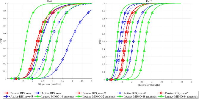
Figure 2: Cumulative distribution function (CDF) of the SE in the case of perfect CSI with $K=8$ and $K=12$. Comparison of the proposed structures in presence of active and passive RIS with legacy MIMO with different numbers of antennas. For the proposed architecture with active and passive RIS we use $N_{A}=16$ and $N_{R}=64$ and for the active RIS we set $\epsilon=20$%.

VI-B Comparison with legacy MIMO

We start contrasting the proposed architecture with a legacy MIMO system using an active antenna array only with fully digital beamforming. In Figs. 2, we show the performance of the proposed RIS-aided architecture for both the cases of active and passive RIS compared with a legacy MIMO system with different number of antennas, for UE’s number $K=8$ and $K=12$. The available power budget $P_{\rm B}$ is used only at the BS active antenna array for the case of legacy MIMO and passive RIS, while for the case of active RIS it is split using $\epsilon=0.2$. Inspecting the figure, it is seen that the proposed architectures well outperform the legacy MIMO system. In particular, for $K=8$, 32 active antennas are needed at the legacy MIMO to outperform the proposed structure with passive RIS (having only 16 active antennas), whereas if an active RIS is used, the proposed structure outperforms (for the directional case corresponding to $\alpha=\pi/5$) the legacy MIMO system even with 64 active antenna arrays and fully digital beamforming. For $K=12$ (en extraordinary load since the proposed structure id using $N_{A}=16$ active antennas) the legacy MIMO system performs relatively better than when $K=8$, but in any case 32 and 48 active antennas are needed to outperform the proposed structure having only 16 active antennas, for the case of passive and active RIS, respectively.

Figure 3: Cumulative distribution function (CDF) of the SE in the case of perfect CSI with $K=8$ and active RIS. Impact of different values of $\epsilon$, i.e., fraction of the power budget allocated to the active RIS in two cases of active antenna array configurations, $\alpha=\pi$ and $\alpha=\pi/5$. We set $N_{A}=16$ and $N_{R}=64$.

VI-C Impact of the fraction of power budget used at the active RIS

In Fig. 3 we study the impact of the fraction $\epsilon$ of power budget used at the active RIS, for two cases of active antenna configurations, i.e., $\alpha=\pi$ and $\alpha=\pi/5$. Again we assume $N_{A}=16$ and $N_{R}=64$. Inspecting the results, it is seen that there is not a big sensitivity of the performance with respect to the choice of $\epsilon$, and the plots suggest that letting $\epsilon=0.5$ may be a reasonably good strategy. The performance sensitivity to $\epsilon$ is also discussed next for the case of imperfect CSI.

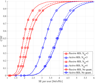
Figure 4: Cumulative distribution function (CDF) of the SE in the case of perfect CSI with $K=8$, $\alpha=\pi/5$ for active RIS and passive RIS. Impact of finite number of RIS states with different values of $N_{Q}$, i.e., number of quantization bits. We set $N_{A}=16$ and $N_{R}=64$ and $\epsilon=20$%.

VI-D Impact of finite number of RIS states

As it is well known, practical RIS can impose on the impinging waves a finite number of admissible phase shifts. To study the effect of such practical constraint, we now assume that the admissible phase shifts (for both active and passive RIS) are quantized over $N_{Q}$ bits. Inspecting Fig. 4, it is seen that there is a noticeable performance degradation when $N_{Q}=3$, especially for the active RIS, while for $N_{Q}=4$ the performance degradation is quite limited.

VI-E Impact of channel estimation

The impact of the channel estimation error on the performance is now assessed using the expressions of the SE lower bounds in Eq. (29) for random configuration of the RIS and in Eq. (28) for the optimized RIS configuration, using numerical evaluation of the statistical expectations. Fig. 5 shows the comparison between the proposed RIS-aided architecture and the legacy MIMO exploiting the hardening lower-bound expressions discussed in Section IV-B. In particular, for the Legacy MIMO, we use the SINR expression in Eq. (29) with $\mathbf{H}=\mathbf{P}=\mathbf{I}_{N_{A}}$. It is seen from the figure that the proposed RIS-aided architecture, for both the cases of passive and active RIS, well outperforms the legacy MIMO because of the highest number of degrees of freedom for the optimization of the system.

Fig. 6 aims at shoing the effectiveness of the proposed optimization procedure for the RIS configuration. In particular, we contrast the case of optimized RIS configuration with the case of random RIS configuration. For the case of random configuration of the RIS we use the SINR expression in Eq. (29), while for the optimized active and passive RIS numerical evaluations of (28) are computed. The figure clearly shows the merits of the proposed optimization procedure, which indeed exhibits impressive gains.

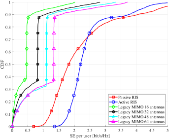
Figure 5: Cumulative distribution function (CDF) of the SE in the case of channel estimation with $K=8$. Comparison of the proposed structures in presence of active and passive RIS with legacy MIMO with different numbers of antennas. For the proposed architecture with active and passive RIS we use $N_{A}=16$, $N_{R}=64$, $\alpha=\pi/5$ and for the active RIS we set $\epsilon=20$%.

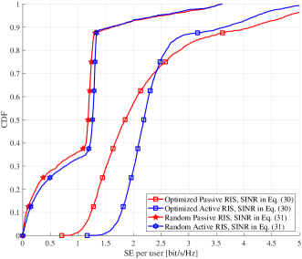
Figure 6: Cumulative distribution function (CDF) of the SE obtained with random and optimized RIS configurations with $K=8$. We set $N_{A}=16$ and $N_{R}=64$, $\alpha=\pi/5$ and for the active RIS we set $\epsilon=20$%.

Finally, in Fig. 7, we report the minimum-SE of the considered architecture versus $\epsilon$, i.e., the fraction of power used at the active RIS. First of all, when $\epsilon=0$%, i.e., no power is used to retransmit signal after the reflection the performance of active and passive RIS is the same, and when $\epsilon=100$% all the power is dedicated to the RIS and the active antenna array has no available power to transmit data, i.e., the communication does not take place. We can see that, especially for directional configuration of active antennas, i.e., $\alpha=\pi/2$ and $\alpha=\pi/5$, the minimum-SE of the UEs increases for values of $\epsilon$ between 10% and 70 %. The approximately flat behaviour in this range is a good indication of the robustness of the proposed system.

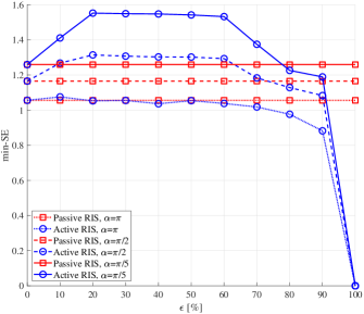
Figure 7: Minimum-SE obtained with optimized RIS configurations versus $\epsilon$ and with different active array antenna configurations. We set $N_{A}=16$ and $N_{R}=64$ and $K=8$.

VII Conclusions

This paper has analyzed a new antenna structure where a (non-large) array of radiating elements is placed at short distance in front of an RIS. For such a structure, and for both the cases of active and passive RIS, we have tackled the topics of channel estimation, downlink transceiver processing, optimization of the RIS configuration, downlink power control, and spectral efficiency bounds derivation. The proposed structure has been compared with a classical legacy MIMO system using an array of active antennas and fully digital beamforming. Interestingly, the results show that the proposed structure is capable of achieving the performance of a legacy MIMO system but with considerably smaller hardware complexity. This paper represents only a first contribution about the design and analysis of such novel structure. This study can be thus generalized along many directions, including the use of more sophisticated beamforming and power allocation schemes, as well as the investigation of its adotpion for localization purposes.

Closed-form Hardening Bound

In this section, we provide the analytical steps to derive (29). We begin by computing the coherent gain term $|\mathsf{DS}_{k}|^{2}$ in (28). Let us define $\overline{\mathbf{P}}=\mathbf{P}\mathbf{H}^{{T}}\mathbf{H}^{*}\mathbf{P}^{*}$, then

$$\mathsf{DS}_{k} \!=\!\mathsf{E}\!\left\{{\bar{\mathbf{h}}^{{T}}_{k}\mathbf{w}_{k}}\right\}=\mathsf{E}\!\left\{{\mathbf{h}_{k}^{{T}}\overline{\mathbf{P}}\widehat{\mathbf{h}}_{k}^{*}}\right\}=\!\mathrm{tr}\!\left(\mathsf{E}\!\left\{{\overline{\mathbf{P}}\widehat{\mathbf{h}}_{k}^{*}(\widehat{\mathbf{h}}_{k}^{{T}}+\widetilde{\mathbf{h}}_{k}^{{T}})}\right\}\right)$$

$$\!=\!\mathrm{tr}\!\left(\overline{\mathbf{P}}\mathsf{E}\!\left\{{\widehat{\mathbf{h}}_{k}^{*}\widehat{\mathbf{h}}_{k}^{{T}}}\right\}\right)\!=\!\mathrm{tr}\!\left(\overline{\mathbf{P}}\mathbf{R}_{\widehat{\mathbf{h}}_{k}\widehat{\mathbf{h}}_{k}}^{*}\right),$$ (45)

where in (45), we use the fact that $\mathsf{E}\!\left\{{\widehat{\mathbf{h}}_{k}^{*}\widetilde{\mathbf{h}}_{k}^{{T}}}\right\}\!=\!\mathbf{0}$, and apply the property $\mathrm{tr}\!\left(\mathbf{X}\mathbf{Y}\right)=\mathrm{tr}\!\left(\mathbf{Y}\mathbf{X}\right)$, for two given matrices $\mathbf{X}$ and $\mathbf{Y}$ matching in size. To compute $\mathsf{E}\!\left\{{|\mathsf{BU}_{k}|^{2}}\right\}$, we first work out the expectations

$$\mathsf{E}\!\left\{{|\widehat{\mathbf{h}}_{k}^{{T}}\overline{\mathbf{P}}\widehat{\mathbf{h}}^{\ast}_{k}|^{2}}\right\} \!\stackrel{{\scriptstyle(a)}}{{=}}\!\left|\mathrm{tr}\!\left(\mathbf{R}^{*}_{\widehat{\mathbf{h}}_{k}\widehat{\mathbf{h}}_{k}}\overline{\mathbf{P}}\right)\right|^{2}\!\!+\!\mathrm{tr}\!\left(\mathbf{R}^{\ast}_{\widehat{\mathbf{h}}_{k}\widehat{\mathbf{h}}_{k}}\overline{\mathbf{P}}\mathbf{R}^{\ast}_{\widehat{\mathbf{h}}_{k}\widehat{\mathbf{h}}_{k}}\overline{\mathbf{P}}^{H}\right),$$

$$\mathsf{E}\!\left\{{|\widetilde{\mathbf{h}}_{k}^{{T}}\overline{\mathbf{P}}\widehat{\mathbf{h}}^{\ast}_{k}|^{2}}\right\} \!=\mathsf{E}\!\left\{{\widetilde{\mathbf{h}}^{{T}}_{k}\overline{\mathbf{P}}\widehat{\mathbf{h}}^{\ast}_{k}\widehat{\mathbf{h}}^{{T}}_{k}\overline{\mathbf{P}}^{H}\widetilde{\mathbf{h}}^{\ast}_{k}}\right\}$$

$$=\mathrm{tr}\!\left(\mathbf{R}^{\ast}_{\widetilde{\mathbf{h}}_{k}\widetilde{\mathbf{h}}_{k}}\overline{\mathbf{P}}\mathbf{R}^{\ast}_{\widehat{\mathbf{h}}_{k}\widehat{\mathbf{h}}_{k}}\overline{\mathbf{P}}^{H}\right),$$

where in $(a)$ we use a well-known identity from random matrix theory (see e.g. [41, Lemma B.14]). By using all previous results, we have

$$\mathsf{E}\!\left\{{|\mathsf{BU}_{k}|^{2}}\right\}=\!\left(\!\mathsf{E}\!\left\{{|\mathbf{h}_{k}^{{T}}\overline{\mathbf{P}}\widehat{\mathbf{h}}_{k}^{*}|^{2}}\right\}\!-\!\left|\mathsf{E}\!\left\{{\mathbf{h}_{k}^{{T}}\overline{\mathbf{P}}\widehat{\mathbf{h}}_{k}^{*}}\right\}\right|^{2}\right)$$

$$\;\stackrel{{\scriptstyle(b)}}{{=}}\!\!\left(\!\!\mathsf{E}\!\left\{{|\widehat{\mathbf{h}}_{k}^{{T}}\overline{\mathbf{P}}\widehat{\mathbf{h}}^{\ast}_{k}|^{2}\!}\right\}\!+\!\mathsf{E}\!\left\{{|\widetilde{\mathbf{h}}_{k}^{{T}}\overline{\mathbf{P}}\widehat{\mathbf{h}}^{\ast}_{k}|^{2}\!}\right\}\!-\!\left|\mathrm{tr}\!\left(\overline{\mathbf{P}}\mathbf{R}_{\widehat{\mathbf{h}}_{k}\widehat{\mathbf{h}}_{k}}^{*}\right)\!\right|^{2}\right)$$

$$\;=\!\!\left(\!\mathrm{tr}\!\left(\mathbf{R}^{\ast}_{\widehat{\mathbf{h}}_{k}\widehat{\mathbf{h}}_{k}}\overline{\mathbf{P}}\mathbf{R}^{\ast}_{\widehat{\mathbf{h}}_{k}\widehat{\mathbf{h}}_{k}}\overline{\mathbf{P}}^{H}\right)\!+\!\mathrm{tr}\!\left(\mathbf{R}^{\ast}_{\widetilde{\mathbf{h}}_{k}\widetilde{\mathbf{h}}_{k}}\overline{\mathbf{P}}\mathbf{R}^{\ast}_{\widehat{\mathbf{h}}_{k}\widehat{\mathbf{h}}_{k}}\overline{\mathbf{P}}^{H}\right)\!\right)$$

$$\;=\!\mathrm{tr}\!\left(\mathbf{R}^{\ast}_{{\mathbf{h}}_{k}{\mathbf{h}}_{k}}\overline{\mathbf{P}}\mathbf{R}^{\ast}_{\widehat{\mathbf{h}}_{k}\widehat{\mathbf{h}}_{k}}\overline{\mathbf{P}}^{H}\right),$$ (46)

where we have again used the trace product property, while $(b)$ is obtained by capitalizing on the zero-mean statistical independency between the LMMSE estimate and the estimation error. Finally, the last equality follows from the fact that $\mathbf{R}_{\widetilde{\mathbf{h}}_{k}\widetilde{\mathbf{h}}_{k}}\!=\!\mathbf{R}_{{\mathbf{h}}_{k}{\mathbf{h}}_{k}}\!-\!\mathbf{R}_{\widehat{\mathbf{h}}_{k}\widehat{\mathbf{h}}_{k}}$.

To compute the term $\mathsf{E}\!\left\{{|\mathsf{UI}_{k,j}|^{2}}\right\}$, we first consider the case in which a pair of UEs $k$ and $j$ share the same pilot sequence, so that (21) holds. Let ${\cal P}_{k}$ denote the set of the indices of the UEs using the same pilot as UE $k$. If $j\in\mathcal{P}_{k}$, then we have

$$\mathsf{E}\!\left\{{|\mathsf{UI}_{k,j}|^{2}}\right\}\stackrel{{\scriptstyle j\in\mathcal{P}_{k}}}{{=}}c^{2}_{j,k}\mathsf{E}\!\left\{{|\mathbf{h}_{k}^{{T}}\overline{\mathbf{P}}\widehat{\mathbf{h}}_{k}^{*}|^{2}}\right\}$$

$$\;=c^{2}_{j,k}\left[\left|\mathrm{tr}\!\left(\overline{\mathbf{P}}\mathbf{R}_{\widehat{\mathbf{h}}_{k}\widehat{\mathbf{h}}_{k}}^{*}\right)\!\right|^{2}\!\!+\!\mathrm{tr}\!\left(\mathbf{R}^{\ast}_{{\mathbf{h}}_{k}{\mathbf{h}}_{k}}\overline{\mathbf{P}}\mathbf{R}^{\ast}_{\widehat{\mathbf{h}}_{k}\widehat{\mathbf{h}}_{k}}\overline{\mathbf{P}}^{H}\right)\right],$$

Conversely, if UE $k$ and UE $j$ are assigned orthogonal pilots, i.e., $j\notin\mathcal{P}_{k}$, then we exploit the statistical independency between $\mathbf{h}_{k}$ and $\widehat{\mathbf{h}}_{j}$ to obtain

$$\mathsf{E}\!\left\{{|\mathsf{UI}_{k,j}|^{2}}\right\} \stackrel{{\scriptstyle j\notin\mathcal{P}_{k}}}{{=}}\mathsf{E}\!\left\{{|\mathbf{h}_{k}^{{T}}\overline{\mathbf{P}}\widehat{\mathbf{h}}_{j}^{*}|^{2}}\right\}=\mathsf{E}\!\left\{{\mathbf{h}_{k}^{{T}}\overline{\mathbf{P}}\widehat{\mathbf{h}}_{j}^{*}\widehat{\mathbf{h}}_{j}^{{T}}\overline{\mathbf{P}}^{H}\mathbf{h}_{k}^{*}}\right\}$$

$$\;\;=\mathrm{tr}\!\left(\mathbf{R}^{*}_{{\mathbf{h}}_{k}{\mathbf{h}}_{k}}\overline{\mathbf{P}}\mathbf{R}^{*}_{\widehat{\mathbf{h}}_{j}\widehat{\mathbf{h}}_{j}}\overline{\mathbf{P}}^{H}\right).$$

Combining the above results, the multi-user interference is

$$\sum\limits_{j\neq k}^{K}\eta_{j}^{(d)}\mathsf{E}\!\left\{{|\mathsf{UI}_{k,j}|^{2}}\right\}=\!\!\!\sum\limits_{j\in\mathcal{P}_{k}\setminus\{k\}}\!\!\eta_{j}^{(d)}c^{2}_{j,k}\left|\mathrm{tr}\!\left(\overline{\mathbf{P}}\mathbf{R}_{\widehat{\mathbf{h}}_{k}\widehat{\mathbf{h}}_{k}}^{*}\right)\!\right|^{2}$$

$$\qquad\qquad+\!\!\!\sum\limits_{j\in\mathcal{P}_{k}\setminus\{k\}}\!\!\eta_{j}^{(d)}c^{2}_{j,k}\mathrm{tr}\!\left(\mathbf{R}^{\ast}_{{\mathbf{h}}_{k}{\mathbf{h}}_{k}}\overline{\mathbf{P}}\mathbf{R}^{\ast}_{\widehat{\mathbf{h}}_{k}\widehat{\mathbf{h}}_{k}}\overline{\mathbf{P}}^{H}\right)$$

$$\qquad\qquad+\sum\limits_{j\notin\mathcal{P}_{k}}\eta_{j}^{(d)}\mathrm{tr}\!\left(\mathbf{R}^{*}_{{\mathbf{h}}_{k}{\mathbf{h}}_{k}}\overline{\mathbf{P}}\mathbf{R}^{*}_{\widehat{\mathbf{h}}_{j}\widehat{\mathbf{h}}_{j}}\overline{\mathbf{P}}^{H}\right).$$ (47)

Finally, if the RIS is active, we need to calculate the power of the dynamic noise

$$\mathsf{E}\!\left\{{|\widetilde{z}_{k}|^{2}}\right\} =\mathsf{E}\!\left\{{|\mathbf{h}_{k}^{{T}}\mathbf{P}\mathbf{z}_{R}|^{2}}\right\}=\mathrm{tr}\!\left(\mathsf{E}\!\left\{{{\mathbf{h}}^{\ast}_{k}{\mathbf{h}}^{{T}}_{k}\mathbf{P}\mathbf{z}_{R}\mathbf{z}_{R}^{H}\mathbf{P}^{H}}\right\}\right)$$

$$=\sigma^{2}_{R}\mathrm{tr}\!\left(\mathbf{R}^{*}_{{\mathbf{h}}_{k}{\mathbf{h}}_{k}}\mathbf{P}\mathbf{P}^{H}\right),$$ (48)

where the last equality follows the statistical independency between $\mathbf{h}_{k}$ and $\mathbf{z}_{R}$. By inserting (45), (VII), (VII) and (VII) into (28), and by using the identity

$$\mathbf{R}^{*}_{\widehat{\mathbf{h}}_{j}\widehat{\mathbf{h}}_{j}}=c^{2}_{j,k}\mathbf{R}^{\ast}_{\widehat{\mathbf{h}}_{k}\widehat{\mathbf{h}}_{k}},$$

which follows from (21), the closed-form SINR expression in (29) is obtained.

References

- [1] S. Buzzi, C. D’Andrea, and G. Interdonato, “RIS-aided massive MIMO: Achieving large multiplexing gains with non-large arrays,” in Proc. of International ITG Workshop on Smart Antennas(WSA), Nov. 2021, pp. 59–64.
- [2] T. L. Marzetta, E. G. Larsson, H. Yang, and H. Q. Ngo, Fundamentals of Massive MIMO. Cambridge University Press, 2016.
- [3] D. W. K. Ng, E. S. Lo, and R. Schober, “Energy-efficient resource allocation in OFDMA systems with large numbers of base station antennas,” IEEE Trans. Wireless Commun., vol. 11, no. 9, pp. 3292–3304, Sep. 2012.
- [4] E. Basar, M. Di Renzo, J. De Rosny, M. Debbah, M.-S. Alouini, and R. Zhang, “Wireless communications through reconfigurable intelligent surfaces,” IEEE Access, vol. 7, pp. 116 753–116 773, Aug. 2019.
- [5] C. Huang, A. Zappone, G. C. Alexandropoulos, M. Debbah, and C. Yuen, “Reconfigurable intelligent surfaces for energy efficiency in wireless communication,” IEEE Trans. Wireless Commun., vol. 18, no. 8, pp. 4157–4170, Aug. 2019.
- [6] Q. Wu and R. Zhang, “Intelligent reflecting surface enhanced wireless network via joint active and passive beamforming,” IEEE Trans. Wireless Commun., vol. 18, no. 11, pp. 5394–5409, Nov. 2019.
- [7] M. Di Renzo, A. Zappone, M. Debbah, M.-S. Alouini, C. Yuen, J. de Rosny, and S. Tretyakov, “Smart radio environments empowered by reconfigurable intelligent surfaces: How it works, state of research, and the road ahead,” IEEE J. Sel. Areas Commun., vol. 38, no. 11, pp. 2450–2525, Nov. 2020.
- [8] Z. Zhang, L. Dai, X. Chen, C. Liu, F. Yang, R. Schober, and H. V. Poor, “Active RIS vs. passive RIS: which will prevail in 6G?” arXiv preprint, Jan. 2022. [Online]. Available: https://arxiv.org/abs/2103.15154
- [9] R. Long, Y.-C. Liang, Y. Pei, and E. G. Larsson, “Active reconfigurable intelligent surface-aided wireless communications,” IEEE Trans. Wireless Commun., vol. 20, no. 8, pp. 4962–4975, Aug. 2021.
- [10] T. V. Chien, H. Q. Ngo, S. Chatzinotas, and B. E. Ottersten, “Reconfigurable intelligent surface-assisted massive MIMO: Favorable propagation, channel hardening, and rank deficiency,” arXiv preprint, Sep. 2021. [Online]. Available: https://arxiv.org/abs/2107.03434
- [11] Q. Wu and R. Zhang, “Beamforming optimization for wireless network aided by intelligent reflecting surface with discrete phase shifts,” IEEE Trans. Commun., vol. 68, no. 3, pp. 1838–1851, Mar. 2020.
- [12] M.-M. Zhao, Q. Wu, M.-J. Zhao, and R. Zhang, “Intelligent reflecting surface enhanced wireless networks: Two-timescale beamforming optimization,” IEEE Trans. Wireless Commun., vol. 20, no. 1, pp. 2–17, Jan. 2021.
- [13] K. Zhi, C. Pan, H. Ren, and K. Wang, “Statistical CSI-based design for reconfigurable intelligent surface-aided massive MIMO systems with direct links,” IEEE Wireless Commun. Lett., vol. 10, no. 5, pp. 1128–1132, May 2021.
- [14] K. Zhi, C. Pan, H. Ren, and K. Wang, “Ergodic rate analysis of reconfigurable intelligent surface-aided massive MIMO systems with ZF detectors,” IEEE Commun. Lett., vol. 26, no. 2, pp. 264–268, Feb. 2022.
- [15] Ö. T. Demir and E. Björnson, “Is channel estimation necessary to select phase-shifts for RIS-assisted massive MIMO?” arXiv preprint, Jun. 2021. [Online]. Available: https://arxiv.org/abs/2106.09770
- [16] A. Abrardo, D. Dardari, and M. Di Renzo, “Intelligent reflecting surfaces: Sum-rate optimization based on statistical position information,” IEEE Trans. Commun., vol. 69, no. 10, pp. 7121–7136, Oct. 2021.
- [17] J. He, K. Yu, Y. Shi, Y. Zhou, W. Chen, and K. B. Letaief, “Reconfigurable intelligent surface assisted massive MIMO with antenna selection,” IEEE Trans. Wireless Commun., pp. 1–1, Dec. 2021, Early Access.
- [18] X. Chen, J. Shi, Z. Yang, and L. Wu, “Low-complexity channel estimation for intelligent reflecting surface-enhanced massive MIMO,” IEEE Wireless Commun. Lett., vol. 10, no. 5, pp. 996–1000, May 2021.
- [19] G. T. de Araújo, A. L. F. de Almeida, and R. Boyer, “Channel estimation for intelligent reflecting surface assisted MIMO systems: A tensor modeling approach,” IEEE J. Sel. Topics Signal Process., vol. 15, no. 3, pp. 789–802, Apr. 2021.
- [20] Z. He, H. Liu, X. Yuan, Y. A. Zhang, and Y. Liang, “Semi-blind cascaded channel estimation for reconfigurable intelligent surface aided massive MIMO,” arXiv preprint, Feb. 2021. [Online]. Available: https://arxiv.org/abs/2101.07315
- [21] A. M. Elbir and S. Coleri, “Federated learning for channel estimation in conventional and RIS-assisted massive MIMO,” IEEE Trans. Wireless Commun., pp. 1–1, Nov. 2021, Early Access.
- [22] Z. Wang, L. Liu, and S. Cui, “Channel estimation for intelligent reflecting surface assisted multiuser communications: Framework, algorithms, and analysis,” IEEE Trans. Wireless Commun., vol. 19, no. 10, pp. 6607–6620, Oct. 2020.
- [23] J. Zhang, C. Qi, P. Li, and P. Lu, “Channel estimation for reconfigurable intelligent surface aided massive MIMO system,” in in Proc. IEEE Int. Workshop on Signal Process. Advances in Wireless Commun. (SPAWC), Aug. 2020, pp. 1–5.
- [24] V. Jamali, A. M. Tulino, G. Fischer, R. R. Müller, and R. Schober, “Intelligent surface-aided transmitter architectures for millimeter-wave ultra massive MIMO systems,” IEEE Open Journal of the Communications Society, vol. 2, pp. 144–167, Jan. 2021.
- [25] X. Mu, Y. Liu, L. Guo, J. Lin, and R. Schober, “Simultaneously transmitting and reflecting (STAR) RIS aided wireless communications,” IEEE Trans. Wireless Commun., pp. 1–1, Oct. 2021, early Access.
- [26] Y. Liu, X. Mu, J. Xu, R. Schober, Y. Hao, H. V. Poor, and L. Hanzo, “STAR: simultaneous transmission and reflection for 360° coverage by intelligent surfaces,” IEEE Wireless Communications, vol. 28, no. 6, pp. 102–109, 2021.
- [27] S. Zeng, H. Zhang, B. Di, Y. Tan, Z. Han, H. V. Poor, and L. Song, “Reconfigurable intelligent surfaces in 6G: Reflective, transmissive, or both?” IEEE Commun. Lett., vol. 25, no. 6, pp. 2063–2067, Jun. 2021.
- [28] K. Ntontin, J. Song, and M. D. Renzo, “Multi-antenna relaying and reconfigurable intelligent surfaces: End-to-end SNR and achievable rate,” arXiv preprint, Aug. 2019. [Online]. Available: https://arxiv.org/abs/1908.07967
- [29] N. T. Nguyen, Q.-D. Vu, K. Lee, and M. Juntti, “Hybrid relay-reflecting intelligent surface-assisted wireless communication,” arXiv preprint, Mar. 2021. [Online]. Available: https://arxiv.org/abs/2103.03900
- [30] J. He, N. T. Nguyen, R. Schroeder, V. Tapio, J. Kokkoniemi, and M. Juntti, “Channel estimation and hybrid architectures for RIS-assisted communications,” in Proc. of Joint European Conference on Networks and Communications and 6G Summit (EuCNC/6G Summit), Jun. 2021, pp. 60–65.
- [31] J.-F. c. Bousquet, S. Magierowski, and G. G. Messier, “A 4-GHz active scatterer in 130-nm CMOS for phase sweep amplify-and-forward,” IEEE Trans. Circuits Syst., vol. 59, no. 3, pp. 529–540, Mar. 2012.
- [32] K. K. Kishor and S. V. Hum, “An amplifying reconfigurable reflectarray antenna,” IEEE Trans. Antennas Propag., vol. 60, no. 1, pp. 197–205, Jan. 2012.
- [33] J. Lončar, A. Grbic, and S. Hrabar, “Ultrathin active polarization-selective metasurface at x-band frequencies,” Phys. Rev. B, vol. 100, p. 075131, Aug. 2019. [Online]. Available: https://link.aps.org/doi/10.1103/PhysRevB.100.075131
- [34] X. Qian and M. Di Renzo, “Mutual coupling and unit cell aware optimization for reconfigurable intelligent surfaces,” IEEE Wireless Commun. Lett., vol. 10, no. 6, pp. 1183–1187, Jun. 2021.
- [35] W. L. Stutzman and G. A. Thiele, Antenna theory and design. John Wiley & Sons, 2012.
- [36] S. Buzzi, C. D’Andrea, A. Zappone, M. Fresia, Y.-P. Zhang, and S. Feng, “RIS configuration, beamformer design, and power control in single-cell and multi-cell wireless networks,” IEEE Transactions on Cognitive Communications and Networking, vol. 7, no. 2, pp. 398–411, Mar. 2021.
- [37] G. Caire, “On the ergodic rate lower bounds with applications to massive MIMO,” IEEE Transactions on Wireless Communications, vol. 17, no. 5, pp. 3258–3268, May 2018.
- [38] D. P. Bertsekas, Nonlinear Programming. Athena Scientific, 1999.
- [39] S. Boyd and L. Vandenberghe, Convex optimization. Cambridge university press, 2004.
- [40] 3GPP, “Study on channel model for frequencies from 0.5 to 100 GHz (Release 16),” 3GPP TR 38.901, Tech. Rep., Dec. 2019.
- [41] E. Björnson, J. Hoydis, and L. Sanguinetti, “Massive MIMO networks: Spectral, energy, and hardware efficiency,” Foundations and Trends® in Signal Processing, vol. 11, no. 3-4, pp. 154–655, 2017.