Broad chemical transferability in structure-based coarse-graining

Abstract

Compared to top-down coarse-grained (CG) models, bottom-up approaches are capable of offering higher structural fidelity. This fidelity results from the tight link to a higher-resolution reference, making the CG model chemically specific. Unfortunately, chemical specificity can be at odds with compound-screening strategies, which call for transferable parametrizations. Here we present an approach to reconcile bottom-up, structure-preserving CG models with chemical transferability. We consider the bottom-up CG parametrization of 3,441 C₇O₂ small-molecule isomers. Our approach combines atomic representations, unsupervised learning, and a large-scale extended-ensemble force-matching parametrization. We first identify a subset of 19 representative molecules, which maximally encode the local environment of all gas-phase conformers. Reference interactions between the 19 representative molecules were obtained from both homogeneous bulk liquids and various binary mixtures. An extended-ensemble parametrization over all 703 state points leads to a CG model that is both structure-based and chemically transferable. Remarkably, the resulting force field is on average more structurally accurate than single-state-point equivalents. Averaging over the extended ensemble acts as a mean-force regularizer, smoothing out both force and structural correlations that are overly specific to a single state point. Our approach aims at transferability through a set of CG bead types that can be used to easily construct new molecules, while retaining the benefits of a structure-based parametrization.

I Introduction

In order to facilitate molecular design for a wide variety of applications, there has recently been a growing interest in utilizing data-driven techniques to infer chemical structure–property relationships that span broad regions of chemical compound space (CCS) [1, 2, 3, 4, 5]. A common rate-limiting step in deriving these relationships is acquiring target properties for a sufficient number of compounds, so as to ensure robustness and transferability. As such, a push for increasingly automated workflows for generating data via both experimental and computational methods has risen in tandem with these data-driven approaches. While experimental approaches are limited due to material cost and ease of chemical synthesis, computational methods do not suffer from these restrictions. Instead, computation is primarily limited by sampling, calling for ever-improving high-performance computing platforms or algorithms [6, 7, 8]. The limitations to computational high-throughput screening often stem from the prohibitive computational cost of simulating large systems (on the order of thousands of atoms) at atomic or electronic resolutions.[9]

A different strategy to computationally screen across more compounds consists of relying on lower-resolution models. Here we focus on particle-based coarse-grained (CG) simulations, in which groups of atoms are mapped to superparticles or beads [10]. The interactions that govern the behavior of these beads aim at recovering the essential physics of the system. This results in simulations that are more computationally efficient due to the reduction in number of particles and a smoothened free-energy landscape. In the context of screening, some CG models offer even more computational efficiency: the CG representation averages over molecules, easing the coverage of CCS. These CG models, commonly called transferable, reduce the size of CCS by making use of a discrete set of CG bead types [11, 12]. Transferable CG models have been used to efficiently cover large subsets of CCS and rapidly sketch structure–property relationships for complex thermodynamic properties [13, 14]. These studies relied on the biomolecular Martini force field, a top-down CG model aiming to reproduce thermodynamic-partitioning behavior in different environments [15]. While top-down CG models can prove extremely efficient to parametrize and extend, they often feature limited structural accuracy [16].

To construct structurally accurate CG models, bottom-up methods offer a more systematic route [17, 18, 19]. They derive CG interactions by matching microscopic information from a higher-resolution reference, for instance the radial distribution function (RDF) or other features of the many-body potential of mean force (MBPMF). The reduction in the number of degrees of freedom makes these target properties inherently dependent not only on the chemical composition, but also the thermodynamic state point. It is thus no surprise that most bottom-up CG studies have focused on individual reference systems. There are various strategies to build bottom-up CG models that are state-point and/or chemically transferable. Intuition can go a long way: different molecules may inspire a consistent CG mapping and set of bead types. For instance, Wang and Deserno parametrized a CG model for phospholipid membranes and showed that the same set of CG beads could be used to construct reliable models for lipids with different saturation levels [20]. In general though, intuition may not be a silver bullet, in particular when bridging across chemical compositions. Van der Vegt and coworkers have demonstrated that an approach based on thermodynamic cycles can provide improved thermodynamic and chemical transferability, with respect to alternative bottom-up methods, subject to the limitations of the form of the interaction potentials.[21, 22, 23] Several groups have used local density-dependent potentials to derive CG models that are transferable across binary mixture concentrations and phases, providing a more accurate description of liquid-vapor interfaces [24, 25, 26, 27, 28, 29]. Sanyal et al. recently developed an extended-ensemble relative-entropy method and constructed a CG protein-backbone model that could accurately reproduce the structures of over 200 different globular proteins [30].

Counter to the expectation that a single model can reproduce the behavior of many different types of systems, transferability may require defining environment-dependent interactions. “Ultra coarse-grained” models are built from a series of internal states [31]. They can accurately model challenging liquid–vapor and liquid–liquid interfaces [32]. CG “conformational surface hopping” applies a simple tuning of the state probabilities to transfer CG models across both state points and chemistry[33, 34]. Other approaches aiming at transferability tend to combine multiple references. For instance, the extended ensemble framework augments the force-matching based multiscale coarse-graining (MSCG) method by averaging over multiple MBPMFs [35]. Mullinax and Noid applied the extended-ensemble approach to build CG potentials of alkanes and alcohols that aim to be transferable across liquid-state binary mixtures [35].

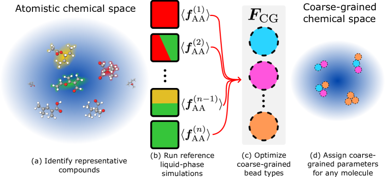
Figure 1: Schematic of our protocol to develop broad chemical transferability in a structure-based coarse-grained (CG) model. (a) Given an atomistic chemical space, identify representative compounds (see Fig. 2); (b) Run reference (atomistic) liquid-phase simulations for various homogeneous liquids and binary mixtures; (c) Optimize a set of CG bead types using an extended-ensemble force-matching scheme; (d) The bead types can readily be used to parametrize any molecule in the (smaller) CG chemical space.

In this work, we extend the scope of bottom-up CG parametrizations to target a significantly larger collection of state points and chemical compositions. Conceptually we seek a CG parametrization scheme that benefits from multiple reference calculations from various parts of chemical compound space. We extend the scope of structure-based and chemically-transferable CG models by simultaneously parametrizing several thousand small organic molecules—the largest bottom-up CG parameterization, to the best of our knowledge. Our data-driven and hierarchical approach is illustrated in Fig. 1. Given a set of chemical compounds, we first identify a small number of “representative compounds,” whose configurational space is best representative of the entire set. Overall our workflow consists of: (a) Using gas-phase conformationally averaged many-body atomic environments, we identify a small number of “representative” molecules; (b) Various atomistic simulations of homogeneous liquids and binary mixtures provide reference mean forces; (c) An extended-ensemble MSCG method simultaneously parametrizes a force field with a small collection of CG bead types over all state points; (d) The set of optimized bead types readily provides nonbonded parameters for all compounds.

We illustrate our approach on 3,441 C₇O₂ isomers found in the Generated Database (GDB) [36, 37]. The identification of 19 representative compounds leads to the generation of 703 atomistic liquids and binary mixtures, used simultaneously to parametrize our CG model. We then quantify the accuracy of the transferable CG model by comparing the RDFs to atomistic references. We also benchmark our transferable model against “traditional” state-point-specific CG force fields.

The results show that enforcing state-point and chemical transferability in CG potentials can yield high structural accuracy. Remarkably, the extended-ensemble parametrization is on average more accurate than state-point specific force fields. Specifically, we find that gains in accuracy are due to a “regularization-like” effect that effectively smooths the average forces acting on specific CG bead types. Averaging over distinct state points and environments reduces the overfitting of system-specific features. Similarly, cross correlations inferred from the atomistic reference simulations are also smoothed, counteracting errors that arise due to the pairwise form of the CG interactions. On the other hand, we also find a few examples where the extended-ensemble model performs notably worse. Low performance stems from certain functional groups that promote vastly different conformational ensembles depending on the environment and molecular topology. An extended-ensemble average over the structural correlations of these functional groups does not capture the specificity of these diverging conformational states, and instead suggests the need for an improved mapping [38, 39, 40] or an increased force-field complexity [41, 42, 33, 43]. We validate the transferability of the derived potentials by running CG simulations on compounds that were not used in the extended-ensemble training set and find that the accuracy of the CG RDFs is on par with that of the representative compounds. Overall, we provide a systematic means to perform a bottom-up coarse-graining over several thousand molecules, resulting in chemically-transferable CG potentials that retain structural accuracy in liquid simulations. At the same time, we highlight the limitations of this approach and note key implementation pitfalls to avoid.

II Methods

II.1 Nomenclature

We first clarify our nomenclature:

• We consider the chemical space of 3,441 C₇O₂ isomers—the entire collection of molecules considered.

• Out of the chemical space considered we focus on 23 molecules. From a clustering analysis, we identify $N_{\rm r}=19$ representative compounds, which are shown in the SI (Figs. S1-S4); 5 additional compounds are selected for validation. Each selected compound and CG mapping are denoted by numbers, where compound numbers run from 0 to 23 (i.e., 0–18 denote the representative compounds, and 19–23 refer to the test compounds). Mapping numbers start from 0 and go up to the handful of possibilities e.g., Molecule 21 with Mapping 0.

• Each of the reference compounds is simulated at an atomistic resolution in a homogeneous liquid and in all considered binary mixtures, leading to $N_{\rm r}(N_{\rm r}+1)/2=190$ reference systems. Systems only refer to the chemical species; as examples, the Molecule 2/Molecule 3 binary system, or the Molecule 10 pure system can be used to describe any simulation containing these particular sets of compounds.

• A state point denotes the particular thermodynamic parameters, including concentration. Specifically, we simulated each binary mixture at 4 different concentrations, corresponding to four state points per system.

• We refer to each combination of system and state point as an ensemble. The aggregate number of homogeneous liquids and binary mixtures of all 19 representative compounds at 4 different concentrations amount to a total of 703 atomistic ensembles simulated for this work.

• Upon coarse-graining, it does not suffice to define the system and state point, but we also need to describe the mapping used, the combination of which we refer to as the mapped ensemble. A single atomistic ensemble may give rise to multiple mapped ensembles, if at least one of the compounds has more than one possible CG mapping. In this work, the 703 atomistic ensembles translate to a total of 2,476 mapped ensembles.

II.2 Database

We selected a subset of the Generated Database (GDB), a computer-generated set of drug-like organic compounds, to test our data-driven bottom-up approach [36, 37]. Specifically, we selected the set of GDB compounds which were made up of seven carbon atoms and two oxygen atoms only. We further filtered out any compounds containing triple bonds. After applying these filters, we were left with a database of 3,441 C₇O₂ isomers, listed in their simplified molecular-input line-entry system (SMILES) format. Despite restricting the size of the molecules and only including three elements (C, O, and H), a large variety is still present in the resulting chemical structures. Furthermore, complex interactions, such as hydrogen-bonding and $\pi$-stacking interactions, are also present for many of the compounds in this database. Because the database was limited in terms of the chemical elements, but still contained compounds which we expected to display complex behavior in the bulk phase, we felt this choice of database would prove useful for determining which specific physical interactions would be (un)successfully captured by our chemically-transferable model.

II.3 Gas-phase simulations

For each compound in the database, we first ran single-molecule gas-phase molecular dynamics simulations. The initial structures were obtained by converting the molecules from their SMILES string representations to energy-minimized 3D conformations using the rdkit package [44]. The force field parameters for each compound were generated using the cgenff tool, included in the silcsbio 2018 package, which automatically assigns parameters from the CHARMM General Force Field based on the input chemistry [45]. The simulations were run at constant volume using a stochastic velocity-rescaling thermostat[46] to maintain a constant temperature, $T=300~{}$K. The simulations were run using a 2 fs timestep for a total of 3 ns, with the LINCS algorithm used to constrain terminal bonds to hydrogen atoms [47]. A frame was output every 2 ps, yielding 1500 frames per simulation for each compound in the database. The gromacs 16.1 package was used to run all of the systems simulated in this work at the atomistic resolution [48].

II.4 Defining local environments with SLATM

The Spectrum of London Axilrod-Teller-Muto (SLATM) vector describes a molecule as a sum of atomic environments that encode the 1-, 2-, and 3-body interactions within a cut-off distance [49, 50]. For each atom, its corresponding SLATM vector consists of the elemental atomic number (1-body), a spectrum of 2-body London interactions convoluted with a gaussian function (2-body), and a spectrum of 3-body Axilrod-Teller-Muto interactions also convoluted with a gaussian function (3-body). The two-body spectrum is computed over the distance as a London interaction between all pairs within a cut-off value with a specified step-size. Similarly, the three-body spectrum is computed as an Axilrod-Teller-Muto interaction over the angle for all triplets within the cut-off distance. We applied the qml package made for python 2.7 to convert our database of compounds into aSLATM representations [51]. The default values, which were optimized for predicting quantum-mechanical properties, were used, with a cutoff value of 0.48 nm and a grid spacing of 0.003 nm and 0.03 radians for the 2-body and 3-body spectra, respectively.

Each frame of the gas-phase simulations yields nine atomic SLATM vectors, i.e., one vector per heavy atom, ignoring hydrogens. Because the number of heavy atoms and chemical composition was constant across the entire database, the length and ordering of the many-body types for each aSLATM vector was the same. Fig. S1 shows the aSLATM vectors of the first molecule over the entire simulation projected into two dimensions using UMAP [52]. There are only four large clusters due to the symmetry of the compound. hdbscan facilitated the identification of clusters in an automated fashion, and seemed relatively insensitive to the choice of hdbscan parameters [53]. The use of different clustering approaches as well as the robustness of the results with respect to the parameters used for these approaches will be the subject of a future study.

II.5 Selecting representative molecules

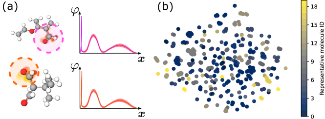
Figure 2: (a) Atomic environments averaged over gas-phase simulations are encoded in aSLATM vectors, $\varphi({\bm{x}})$. (b) UMAP projection of the averaged aSLATM vectors for the 3,441 C₇O₂ isomers. Points colored according to one of the 19 representative molecules.

All of the gas-phase aSLATM cluster centers were combined and clustered using hdbscan. We used the default hdbscan parameters, with both the minimum cluster size and number of nearest neighbors set to five points. Fig. 2b shows a UMAP projection of this data set colored by the identified representative molecules. It clearly shows that the set of representative covers the conformational space of all compounds. The UMAP projection (set using the default parameters) is used only for visualization purposes, while the identification of clusters was performed in the high-dimensional aSLATM space. Beyond the overall separation of aSLATM vectors based on chemical element, no other global trends are seen across the various clusters defined. Although we only provide labels for a small fraction of the clusters identified in Fig. 2, we saw that most of the distinct clusters that are present in the UMAP projection are also labeled as distinct clusters according to our hdbscan results on the high-dimensional data. Because we were also able to identify the key chemical motifs that define these clusters via visual inspection, we are confident in the accuracy of the clustering results. We then chose representative molecules by first ranking them by the number of clusters “visited,” meaning we prioritized the compounds with aSLATM vectors belonging to as many different clusters as possible. We then included subsequent molecules if the number of new clusters visited by the molecule was greater than the number of clusters already visited by the other chosen molecules. By applying this simple algorithm, we found 19 molecules containing local environments that shared cluster assignments with over 92% of the assigned aSLATM vectors. These nineteen representative molecules, shown in Figs. S1-S4, were then used as the foundation for our extended-ensemble approach.

II.6 Atomistic simulations of bulk liquid-phase binary mixtures

An extended ensemble consisting of bulk liquid-phase molecular dynamics simulations of each of the 19 representative molecules, as well as binary mixtures of the representative molecules, was constructed. Each system consisted of 400 molecules in total, with the concentrations for compounds in the binary mixtures ranging from 20% to 80% in 20% increments. Therefore, the total number of state points simulated at the atomistic resolution was 703: 19 pure liquids plus every possible combination of binary mixtures, each simulated at the four different concentrations.

Each of these 703 systems was simulated using the following protocol, adapted from the procedure used by Dunn and Noid [54]. 400 molecules were first randomly placed into an isotropic box with a volume of 1000 nm³. The system was energy-minimized and then run in the $NVT$ ensemble using a velocity-rescaling thermostat for 2 ns at a temperature of 1000 K [46]. The system was then cooled to 300 K over the course of the next 10 ns. At this point the Berendsen thermostat and barostat were used to reduce the size of the box and equilibrate the system in the $NPT$ ensemble at 300 K and 1 bar [55]. The resulting densities ranged from $\approx 0.80$ g/cm³ to $\approx 1.0$ g/cm³. While no specific density data could be obtained for these 19 representative molecules, these densities roughly agree with those of 1,7-heptanediol (0.95 g/cm³), heptanoic acid (0.92 g/cm³), and pentyl acetate (0.87 g/cm³), which also consist of 7 carbon and 2 oxygen atoms [56]. In a similar vein, we were unable to find previously-reported isothermal compressibilities for these specific compounds, and used the isothermal compressibility of heptanoic acid, $7.4\cdot 10^{-5}$ bar^-1 for all systems [57]. Production runs were then carried out under these conditions in the $NPT$ ensemble using the Nosé-Hoover thermostat and the Parinello-Rahman barostat with coupling constants of $\tau_{T}=0.5$ ps and $\tau_{P}=5.0$ ps, respectively [54]. The force field parameters used were the same as those used in the gas-phase simulations, with LINCS constraints applied to the hydrogen-to-heavy-atom bonds. The final trajectories consisted of 60 ns simulations of each system, of which the first 5 ns were discarded to allow for equilibration after applying the new thermostat and barostat.

II.7 Applying the multi-scale coarse-graining technique

We briefly outline the MSCG method here, but refer the reader for a more in-depth description [58, 59, 60, 61, 10, 62]. The first step in the coarse-graining process is to define a mapping function from atoms to CG beads [10]. The loss of resolution makes the mapping choice an important one, although, in practice, this is often based on chemical intuition alone. The analysis of the clusters shown in Fig. 2 naturally points to a mapping scheme corresponding to functional groups. As a result, we adopted a mapping scheme in which all combinations of two- and three-heavy-atom fragments consisting of carbon and oxygen are assigned to different bead types, as shown in Table 1. In order to ensure completeness of our training set—all heavy atoms are assigned to a bead type and the topology of the fragments are preserved—we also included two fully-branched bead types mapping to four-heavy-atom fragments. This set of bead types led to mapping degeneracy for a number of molecules, i.e., they can be mapped in multiple ways. The full set of compounds and associated CG mappings is shown in Fig. S1. Although the cartoon mappings shown in these figures in some cases depict the beads as being ellipsoidal, the potentials assigned to each bead type are radially symmetric (corresponding to a spherical shape).

CG Type	Fragment	CG Type	Fragment	CG Type	Fragment
B01	CC	B06	CCO	B11	C=CO
B02	CO	B07	COC	B12	OC=O
B03	C=C	B08	OCO	B13	C(C)(C)C
B04	C=O	B09	CC=C	B14	C(C)(C)O
B05	CCC	B10	CC=O

Table 1: Bead types and their corresponding fragments in SMILES notation.

We now turn to determining the CG potential. In order to maintain thermodynamic consistency condition across both CG and atomistic systems, the marginal probabilities over the CG degrees of freedom between the CG model and reference atomistic simulations must be equal.[60, 10] Under this condition, solving for the CG force field yields a projection of the atomistic free-energy surface onto the CG degrees of freedom, known as the MBPMF [10]. We use the MSCG approach to variationally determine a CG potential that best approximates the MBPMF [18]. The variational principle ensures that the resulting CG potential best reproduces the averaged atomistic net force acting on CG sites. For this reason, the MSCG approach is also commonly referred to as the force-matching method for bottom-up coarse-graining. The high-dimensional MBPMF is often projected onto molecular mechanics terms commonly used in atomistic MD, including nonbonded pairwise contributions. Due to the inherently many-body nature of the MBPMF, the use of pairwise interactions in the CG force field, while computationally convenient, usually introduces some degree of error due to the projection of many-body effects onto a pairwise basis. However, in this work, we limit ourselves to pairwise non-bonded interactions between the different bead types, represented using a set of flexible spline functions as a basis set. If the CG forces depend linearly on the parameters of the model, ${\bm{\phi}}$, then the MSCG method corresponds to a linear least-squares problem in these parameters. This optimization problem can equivalently be expressed as a coupled set of linear equations (i.e., the normal equations):

$$\sum_{D^{\prime}}G_{DD^{\prime}}\phi_{D^{\prime}}=b_{D},$$ (1)

where $D$ denotes a single interaction type at a specified distance. In this equation, the correlation matrix, $G_{DD^{\prime}}$, measures the cross-correlations between all atomistic interactions when projected onto the force-field basis vectors defined. $b_{D}$ is a vector obtained by projecting the MBPMF of the atomistic reference onto these force field basis vectors. Solving equation 1 yields the parameters $\phi_{D^{\prime}}$ corresponding to the CG potential that minimizes the force-matching functional.

We used the bocs software package developed by Dunn et al. to apply the MSCG method to each of the 703 atomistic ensembles in the extended ensemble [63]. For systems made up of compounds with multiple mappings, we systematically applied every possible mapping (or combination of mappings in the case of binary mixtures) and calculated the MSCG potential from each mapped atomistic trajectory. We first applied the direct Boltzmann inversion method in order to obtain intramolecular (i.e., “bonded”) CG potentials. In cases where certain angle and dihedral values were not sampled, we modified the resulting potential to include large barriers, effectively preventing the CG systems from sampling these values. To properly account for the contribution of these intramolecular interactions to the mean force, we explicitly calculated the contributions and subtracted them before solving equation 1 [64], including only the nonbonded and bond interactions. Although the bond interactions are included in the calculation, we do not update the corresponding forces (i.e., the Boltzmann-inverted bond potentials are used for all simulations). Previous work has suggested that the inclusion of the bond interactions, even after subtracting their contribution to the mean force, can provide numerical stability for determining optimal nonbonded parameters [65, 66, 67]. All pairwise interactions were represented with radially-isotropic fourth-order basis splines with control points spaced every 0.01 nm ranging from 0.0 to 1.4 nm. In this fashion, a set of CG pairwise potentials was generated for each mapping at each state point. This protocol was applied using an automated framework, and, to the best of our knowledge, this is the first study in which such a large number of systems has been systematically coarse-grained using the MSCG method.

II.8 Averaging over the extended ensemble

Mullinax and Noid proposed the extended-ensemble MSCG framework, which extends the variational principal of the MSCG method to determine the optimal approximation to a generalized MBPMF, constructed from a number of system-dependent MBPMFs [35]. Within the extended ensemble, the average of an observable, $\langle A\rangle$, is evaluated as

$$\langle A_{\Gamma}(\bm{R}_{\Gamma})\rangle=\sum_{\Gamma}^{N_{\Gamma}}P_{\Gamma}\langle A_{\Gamma}(\bm{R}_{\Gamma})\rangle_{\Gamma},$$ (2)

where $\Gamma$ specifies the molecular identity, CG mapping, and thermodynamic state point of a single system within the extended ensemble (i.e., a mapped ensemble as previously defined), ${\bm{R}_{\Gamma}}$ represents the cartesian coordinates of system $\Gamma$, and $N_{\Gamma}$ is the total number of systems making up the extended ensemble. $P_{\Gamma}$ is the weight of system $\Gamma$, and is taken to be $1/N_{\Gamma}$ in this work. $\langle\cdot\rangle_{\Gamma}$ denotes the usual ensemble average within system $\Gamma$, and implies the appropriate conditional averaging for observables evaluated from atomically-detailed simulations. Similarly to the original MSCG framework, the optimal CG force field parameters, ${\bm{\phi}}$, within the extended ensemble can be determined by solving Equation 1, while evaluating the correlation functions according to Equation 2 [35, 63].

In practice, we first initialize a correlation matrix $G_{DD^{\prime}}$ and mean force vector $b_{D}$ for all 105 pairwise interactions between the 14 bead types that we have defined as well as all bonded interactions (to ensure numerical stability). With all elements initially set to zero, we then iterate over all of the mapped ensembles, adding each of the blocks of the correlation matrix and segments of the mean force vector for a single state point to the corresponding block and segment in the extended ensemble correlation matrix and mean force vector, respectively. As multiple mappings can exist for a single ensemble, we use the same atomistic trajectory multiple times to efficiently obtain correlations. For example, Fig. 5b shows that Molecule 21 has two different mappings, labeled mapping 0 and mapping 1. Although the number and type of beads does not change, the way in which the atomistic fragments are mapped to these beads does change. In this case, two distinct sets of pairwise interaction statistics for the same interactions from a single atomistic trajectory are obtained. In addition to the Molecule 21 case, Fig. S1 shows several different mappings that are applied to the same compound, similarly allowing for additional correlations to be included without generating additional atomistic trajectories. After inlcuding the correlations from each of these mapped ensembles to $G_{DD^{\prime}}$ and $b_{D}$, we compute the average by dividing by the total number of mapped ensembles as required by Equation 2. Using the bocs software package, we solved Equation 1 with the extended ensemble correlation matrix and mean-force vector.

II.9 Validation and quantifying structural accuracy

Once we have obtained our CG potentials, we compare state-point (SP) specific CG potentials to the extended-ensemble (EE) potentials. Both approaches share the same intramolecular potentials. The CG simulations are run in the $NVT$ ensemble using an isotropic box that has dimensions matching the average density calculated from the atomistic state-point trajectory. A time step of $\delta t=0.002~{}\tau$ was used for all simulations, where $\tau$ is the natural time unit for the propagation of the model defined in terms of the units of energy $\mathcal{E}=1$ kJ/mol, mass $\mathcal{M}=1$ amu, and length $\mathcal{L}=1$ nm, as $\tau=\mathcal{L}\sqrt{\mathcal{M}/\mathcal{E}}$. The simulations were run for $5\times 10^{6}$ time steps, with every 500^th frame saved as output, and the first 500 output frames were discarded. The gromacs 5.1 package was used to run all CG simulations in this work [68]. We observed a speed-up factor of $\approx 3.0$ when comparing the CG to the atomistic simulations (with the CG simulations running at $\approx 0.35$ ns/CPU hour).

To assess the effectiveness of the EE potentials, we first compare radial distribution functions (RDFs), $g(r)$, between the different models. We quantify the agreement between the CG and atomistic RDFs using the Jensen-Shannon divergence (JSD) [69]. Divergences relating two functions have successfully been used in the context of the relative-entropy framework as a useful tool for evaluating the quality of CG models [70, 71]. We previously used the JSD to evaluate the CG distribution of water/octanol partitioning free energies across small organic molecules,[12] as well as force-field accuracy within the conformational surface hopping scheme.[34] While the Kullback-Leibler divergence, $D_{\mathrm{KL}}$, [72] directly relates two distributions, the JSD computes the relative entropy by comparing each of these distributions to the average of the other two

$$D_{\mathrm{JS}}=\frac{1}{2}D_{\mathrm{KL}}\left(g_{\mathrm{CG}}(r)||g_{\mathrm{avg}(r)}\right)+\frac{1}{2}D_{\mathrm{KL}}\left(g_{\mathrm{AA}}(r)||g_{\mathrm{avg}}(r)\right),$$ (3)

where

$$D_{\mathrm{KL}}(g_{\mathrm{A}}(r)||g_{\mathrm{B}}(r)) =\sum_{r=0}^{r_{\rm max}}g_{\mathrm{A}}(r)\ln\left(\frac{g_{\mathrm{A}}(r)}{g_{\mathrm{B}}(r)}\right),$$

$$g_{\mathrm{avg}}(r) =\frac{1}{2}(g_{\mathrm{CG}}(r)+g_{\mathrm{AA}}(r)).$$

In the above equations, we define $D_{\mathrm{KL}}$ in terms of two arbitrary RDFs, $g_{\mathrm{A}}(r)$ and $g_{\mathrm{B}}(r)$ ranging from $r=0$ to $r_{\rm max}$. For all RDFs, we used a grid spacing of 0.01 nm and $r_{\rm max}=1.5$ nm. All RDFs were calculated using the gmx rdf package included in gromacs 5.1. The JSDs for both the SP and EE are compared to their respective atomistic RDFs.

II.10 Mean Force Decomposition Analysis

Equation 1 can be transformed to depend only on structural information, revealing the set of equations as a generalization of the Yvon-Born-Green integral equation framework from liquid state theory [73, 74]. Within this formulation, for a single pairwise-additive distance-dependent interaction represented with a set of piecewise constant basis functions, ${\bm{b}}$ corresponds to a structural correlation function that is directly related to the radial distribution function (RDF):

$$b_{D}=k_{\rm B}TcR_{D}^{2}\left(\frac{{\rm d}{\bm{g}}}{{\rm d}R}\right)_{\!\!D}\,\,,$$ (4)

where $c=(4\pi N)/(3V)$ and $\bm{g}$ is the discretization of the RDF implied by the basis function representation. $\left({\rm d}{\bm{g}}/{\rm d}R\right)$ is meant as a numerical derivative of $\bm{g}$ with respect to interparticle distance $R$, given by the basis function centers $\{R_{D}\}$.

The correlation matrix ${\bf G}$ also has a clear physical interpretation [75]. First, it is useful to decompose ${\bf G}$ into two matrices which, through Equation 1, determine the direct and indirect contributions to ${\bm{b}}$:

$$G_{DD^{\prime}}=\bar{g}_{D}\delta_{DD^{\prime}}+\bar{G}_{DD^{\prime}}\,\,,$$ (5)

where $\delta_{DD^{\prime}}$ is the Kronecker delta function. The direct contribution $\bar{\bm{g}}$ is a correlation function that is again related to the RDF: $\bar{g}_{D}=cR_{D}g_{D}$. $\bar{{\bf G}}$, on the other hand, quantifies the cross correlations between pairs of interactions, in this case the average cosine of the angle formed between triplets of CG sites [75]. Equation 4 clearly implies a relationship between $b(R)$ and the pair mean force, $-w^{\prime}(R)=-\frac{\rm d}{{\rm d}R}[-k_{\rm B}T\ln g(R)]$. Thus, using Equation 5, the pair mean force can be decomposed into direct and indirect contributions:

$$-w^{\prime}_{D}=\frac{b_{D}}{\bar{g}_{D}}=\phi_{D}+\frac{1}{\bar{g}_{D}}\sum_{D^{\prime}}\bar{G}_{DD^{\prime}}\phi_{D^{\prime}}\,\,.$$ (6)

III Results

In this work, we construct a chemically-transferable and structurally-accurate CG model for C₇O₂ isomers, following a bottom-up approach. The model was parametrized using an “extended ensemble” of 703 atomistic reference ensembles of pure liquids and binary mixtures, consisting of 19 representative compounds determined by clustering the gas-phase conformation-averaged atomic SLATM vectors of 3,441 C₇O₂ isomers. The parametrization also included multiple CG mappings for individual reference systems, resulting in 2,476 mapped ensembles in total (see Fig. S1).

In the following, the extend ensemble (EE) model is assessed through comparisons of RDFs to both the reference atomistic ensembles (at the CG level of resolution) and also to state-point specific (SP) models, i.e., models constructed using individual reference simulations. SP and EE parametrizations share all intramolecular (i.e., bond, angle, and dihedral) interactions, obtained by direct Boltzmann inversion of the pure-liquid simulations. Each of the 2,476 mapped ensembles contains up to 28 RDFs, making a manual inspection unfeasible (although all EE RDFs are available online [76]). Note that while the atomistic simulations were run in the $NPT$ ensemble, the CG simulations were run in the $NVT$ ensemble, with the volume of the simulation box equal to the average volume of the atomistic simulation box. We assess the relative error of the CG models at a density corresponding to the atomistic reference. We use JSD values to quantify the accuracy of the SP and EE CG RDFs relative to the atomistic RDFs. Fig. S2 provides several examples of RDF comparisons that result in certain JSD values, a useful reference for interpreting these JSD values in terms of the error when comparing atomistic and CG RDFs. Fig. 3 reports the distribution of JSD values for all 36 homogeneous liquids (see Fig. S3 for the state-point averaged JSDs per system). Also shown in this figure are the mean of both the SP and EE CG models. One might expect the EE model to perform worse than the SP models because the EE model is obtained by averaging over many different reference ensembles, rather than optimizing the model for any particular one. Remarkably, on average, the transferable EE model outperforms the SP models with an average JSD value of 0.0024 versus 0.0038, respectively. The EE distribution is also narrower, indicating more regularity in the quality of the CG parametrizations. We find several state points where the EE model greatly outperforms the SP model: Molecule 3 mapping 0, Molecule 8 mapping 0, Molecule 1 mapping 0, see Fig. S3. On the other hand, we also find opposite cases: Molecule 6 mapping 0 and Molecule 5.

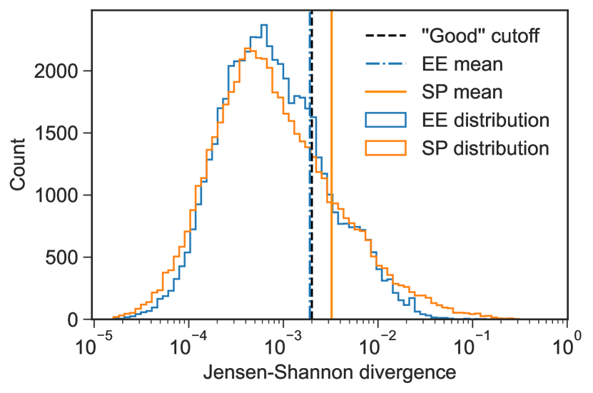
Figure 3: Distribution of JSD values using both the state-point specific (orange) and transferable extended-ensemble (EE; blue) models. The black dashed line denotes the cutoff JSD value for “good” agreement with atomistic RDFs, 0.002.

We now change perspective: we analyze the same set of systems and RDFs, but average according to interaction types. Fig. 4 presents a matrix-form heat map of JSD values, with column-row combinations representing interaction pairs. The lighter coloring of the EE interactions conveys the same message as before: EE CG models are on average closer to the atomistic reference, and the SP CG models show more outliers. The use of a logarithmic scale emphasizes strong deviations. While most of the EE RDFs are significantly below the “good” agreement JSD cutoff, the previous averaging over systems leads to larger JSD values (Fig. S3). The difference in the tails of the SP and EE distributions in Fig. 3 highlights the dominating effect of a few interaction types.

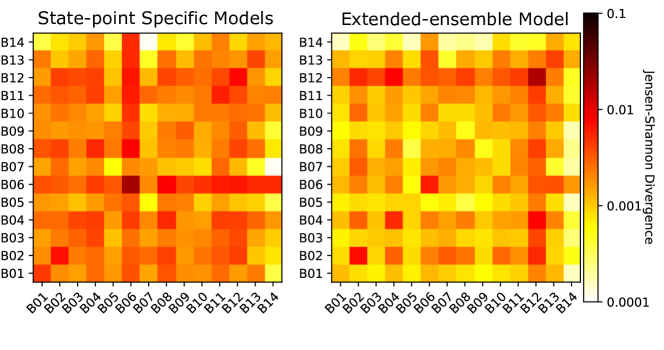
Figure 4: JSD values of interactions sampled in pure, homogeneous liquids using both the state-point (SP) specific and transferable extended-ensemble (EE) CG models on the left and right panels, respectively.

We now investigate the transferability of the EE model beyond the set of representative molecules, but within the considered chemical space of 3,441 C₇O₂ isomers. “Test” compounds are selected based on their molecular SLATM distance from the training compounds. The molecular SLATM vector simply consists of the sum of aSLATM vectors in a molecule. We quantify compound similarity from the 3,441 isomers to the 19 representative molecules by means of a matrix of pairwise Euclidean distances between molecular SLATM representations. To focus on molecules that share as little information as possible from the pool of representative molecules, we focus on the largest average distances. Tab. 2 reports the SMILES string of the five furthest compounds, as well as their scaled SLATM distance (i.e., the maximum Euclidean distance is 1.0).

Molecule	SMILES string	Scaled SLATM distance
Index		from training set
19	CCC(CC)OC(C)=O	0.43
20	CC(C)=CC(=C)C(O)=O	0.48
21	C=COC(=C)C(=C)C=O	0.88
22	CC(C)(C)C(C=O)C=O	0.91
23	CC(C)C(C)(C=O)C=O	0.91

Table 2: Test molecules, SMILES strings, and SLATM distance to the representative molecules scaled by the maximum distance.

The performance of the CG models for the test molecules, as well as an illustration of their mappings, is shown in Fig. 5. In analogy to Fig. 3, we average the JSDs of the SP and EE CG RDFs for each system. We find that the largest improvement from SP to EE parametrization corresponds to Molecule 19—the closest compound to the representative set. It confirms that a larger conformational overlap can benefit the transferable-parametrization strategy. Other factors also play a role, as indicated by the superior and comparable performance of the EE model for Molecules 23 and 21, respectively, despite these molecules being further away from the representative set on average (see Table 2). On the other hand, the EE model underperforms compared to the SP model for Molecules 20 and 22. While Molecule 22 is also one of the furthest compounds on average from the representative set, Molecule 20 is only slightly further than Molecule 19. We defer a rationalization of the results for these compounds to later in the text. Evidently, an analysis of five molecules is by no means statistically representative of the chemical space considered. However, this provides a glimpse of the behavior of the EE model for molecules with varying conformational overlap.

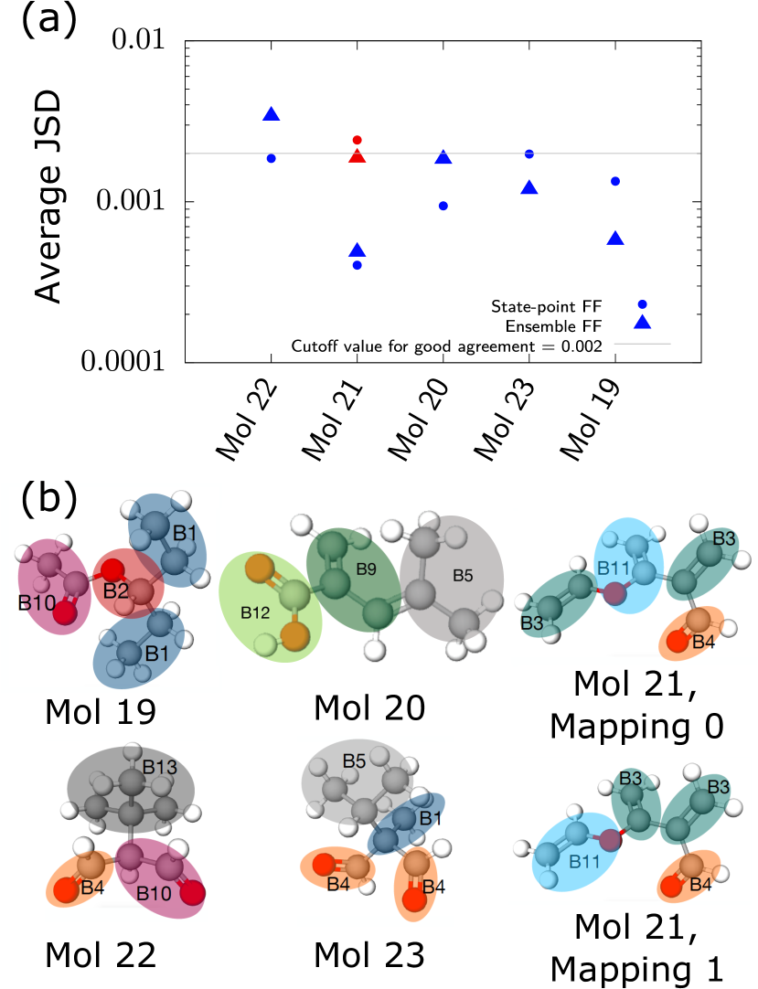
Figure 5: Average JSD values of bulk liquid MD simulations for five test compounds, displaying both SP (circles) and EE (triangles) CG models. Molecule 21 has two mappings, shown in different colors. The grey line denotes the cutoff JSD value for “good” agreement with atomistic RDFs, 0.002. The molecules are ordered based on increasing agreement of the atomistic RDFs with the EE CG RDFs.

IV Discussion

Our results show that an extended-ensemble (EE) parametrization across a wide set of small organic isomers leads to more accurate and consistent CG models. This was demonstrated in Fig. 3, where the distribution of EE JSD values shows a smaller mean and variance than the state-point specific (SP) models. These results might be counterintuitive, in that a force field that is parametrized using information averaged over many simulations is expected to perform worse than another of equal complexity that focuses on a particular reference ensemble. Instead the results indicate that better transferability can go hand in hand with improved accuracy. Beyond this overall improved accuracy, the reduced variance of the JSD distribution indicates that the EE model will result in more reliable predictions. On the other hand, our analysis also reveals cases where the EE model underperforms, compared to a more traditional SP parametrization. To better understand the advantages and pitfalls of the EE parametrization, we investigate certain ensembles and the corresponding mapped ensembles where the EE and SP models lead to significant differences.

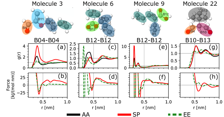
Figure 6: Atomistic and CG RDFs of pure-liquid simulations and pairwise forces for molecules (a-b) 3, (c-d) 6, (e-f) 9, and (g-h) 22, respectively. The black, red, and green curves denote respectively the atomistic, SP, and EE RDFs for the fragments which map to the bead types listed in the top-right of each plot.

We first consider the pure Molecule-3 system. Mapping 0, depicted in the molecular image at the top of Fig. 6, shows the greatest structural improvement from SP to EE parametrization, according to the average JSD value (Fig. S3). An example RDF for the B04–B04 interaction is shown in Fig. 6a, and the RDFs pertaining to all other pairwise interactions are available in the SI (See Fig. S5). The SP model (solid red curve) drastically overstabilizes the first and second solvation peaks of the B04–B04 RDF, while the EE model (dashed green curve) better reproduces the AA simulation, with a mild understabilization of the solvation structure. Fig. 6b presents the B04–B04 pair forces for the SP and EE models. Both forces exhibit similar features within the first solvation shell region, with minima at $r\approx 0.4$ nm. However, the EE force demonstrates a significant reduction of the magnitude of repulsive forces beyond this minimum. Overall we found that the magnitude of these repulsive features were always either maintained or reduced in the EE model with respect to the SP model, and were rarely seen to increase in the EE case. The repulsive nature of the SP forces is consistent with previous work showing that structure-based CG approaches tend to result in models with overly repulsive potentials.[77, 78, 54, 34]. Compared to the SP models, the EE forces tend to look simpler—qualitatively more similar to a Lennard-Jones form. A similar finding was reached when augmenting a CG model with multiple, conformationally dependent force fields [34]. The results suggest that solving Equation 1 over the extended ensemble promotes a regularization effect, which accounts for correlations across conformational and chemical space. Averaging over these correlations appears to have the net effect of smoothening sharp, localized features in the mean force while preserving the key features shared across the extended ensemble.

Next, we examine cases where the EE model underperforms compared to the SP model. Fig. 4 shows that the EE B12–B12 interaction, found in molecules 6, 9, and 16 (see SI Fig. S5), is significantly worse when compared to the SP model, with average JSD values of 0.018 and 0.008, respectively. Panels (c) and (d) of Fig. 6 present the SP and EE B12–B12 RDFs and forces, respectively, for molecule 6. Panels (e) and (f) show the corresponding quantities for molecule 9. In contrast to the B04–B04 interactions of molecule 3, the repulsive bumps at $r\approx 0.6$ nm are retained within the EE model, suggesting that they are essential for stabilizing the proper structure. Both the SP and EE forces for molecule 9 contain a sharp attractive feature at $r\approx 0.3$ nm, which are clearly responsible for the corresponding sharp crystalline peaks in the RDFs at this distance. A similar feature is found in the EE force for molecule 6, although there is no corresponding feature for the SP model. We conclude that the extended-ensemble averaging “transferred” this particular trait from molecule 9 to others—including molecule 6, resulting in significant errors in the RDFs for this interaction type. Overall, we find that within the EE approach interactions involving B12 average over significantly different local environments. Indeed, the atomistic RDFs of molecules 6 and 9 display pronounced differences. The sharp peaks observed in molecule 9 clearly indicate liquid-crystalline behavior, absent in the molecule 6 liquid. This is expected: molecule 9 consists of alternating single and double bonds facilitating $\pi$-stacking interactions, a clear promoter of liquid crystals for organic small molecules [79, 80]. Furthermore, the presence of a terminal carboxylic-acid group encourages hydrogen bonding in the bulk-liquid phase, which also promotes ordering. On the other hand, the B12 bead in molecules 6 and 16 represents ester groups, which lack hydrogen bonding, and also lack conjugated bonds for $\pi$-stacking. Our use of a single bead type to represent such different chemical environments results in a CG potential that cannot faithfully reproduce either case. Furthermore, the strong anisotropic character of $\pi$-stacking and hydrogen-bonding interactions may call for potentials that go beyond pairwise and isotropic functions.[81, 82] We foresee that improvements in the CG mapping and/or the CG force-field complexity would help remedy the situation. While the reuse of atomistic trajectories to generate multiple mapped ensembles allows for an efficient way to obtain correlations and forces to average over using the EE approach, failing to account for these differences in atomic environments can lead to an exacerbation, rather than a reduction, of undesirable features in the resulting forces.

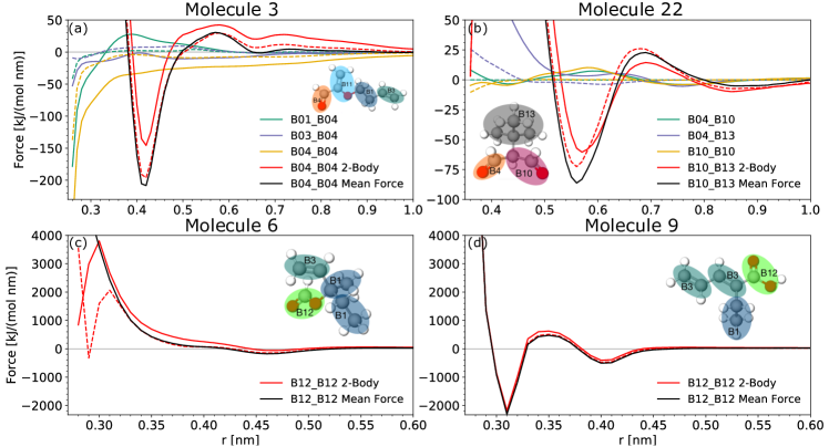
Figure 7: Mean forces (black curves) for the interactions corresponding to the RDFs shown in Fig. 6. For (a) and (b), the three of the three-body contributions to the mean force for both the SP (solid) and EE (dashed) models are shown. For (c) and (d), The two-body contributions to the B12-B12 mean force for the SP (solid) and EE (dashed) models are shown.

To further understand the apparent regularization effect that arises due to averaging correlations within the extended ensemble, we performed an analysis of the mean forces for the pure liquid systems of the four molecules presented in Fig. 6 (representative Molecules 3, 6, and 9, and test Molecule 22). Following Section II.10, we first decomposed the SP mean forces into contributions from each of the interactions in the system, using the cross-correlations calculated from the corresponding reference ensemble. The solid curves in Panel (a) of Fig. 7 present the resulting decomposition for the B04–B04 interaction of molecule 3, for a subset of the contributions. The remaining contributions have negligible impact on the B04–B04 mean force (solid black curve). The solid red curve represents the direct, or 2-body, contribution (i.e., the SP B04–B04 pair force). The other colored solid curves represent 3-body contributions (i.e., correlated contributions to the B04–B04 mean force from a particular distinct interaction). By definition, the sum of 2- and 3-body contributions equal the total mean force (Eq. 6). Thus, in this case, it is apparent that, while the 2-body contribution is dominant, there are significant contributions from other interactions, both within the first solvation shell and beyond. Panel (b) of Fig. 7 presents the corresponding result for the B10–B13 interaction of molecule 22, with similar overall features to the B04–B04 case.

To directly probe the impact of averaging correlations over distinct environments, we repeated the decomposition of the SP mean forces using EE correlations instead of the SP correlations. The results are presented as the dashed curves in panels (a) and (b) of Fig. 7. For both molecules 3 and 22, there is a reduction in the magnitude of the 3-body contributions to the mean force, as might be expected due to smoothing of correlations via the EE averaging. This can be most clearly seen in the similarity between the 2-body contributions (dashed red curves) and the total mean force (solid black curves). To interpret these results, it helps to reconsider the g-YBG equations. Eq. 1 represents an exact relationship between the force field parameters ${\bm{\phi}}$ and the structural correlation functions ${\bm{b}}({\bm{\phi}})$ for a single state point, determined from molecular simulations, via the cross correlations, ${\bf G}({\bm{\phi}})$, generated by the same model ${\bm{\phi}}$. In contrast, the MS-CG method attempts to predict the force-field parameters ${\bm{\phi}}$ that will reproduce ${\bm{b}}^{\rm AA}$, using ${\bf G}^{\rm AA}$ as a proxy for the cross correlations of the CG model [65, 66]. While ideally ${\bf G}^{\rm AA}={\bf G}({\bm{\phi}})$, limitations in the CG basis set can only approximately reproduce the AA correlations. The EE scheme populates the correlation matrix with complementary contributions from various systems and state points. Incorporating more reference simulations could improve the state-point parametrization, by smoothing out correlations that are too complicated for the CG model to reproduce. However, this numerical experiment represents only a portion of the extended ensemble calculation, which additionally performs an average over the various mean forces, i.e., through the average over the ${\bm{b}}^{\rm AA}$ coefficients for each system and state point. It is apparent from the analysis in Fig. 7 that the smoothing of correlations is not responsible for the lack of repulsive features in the EE forces beyond the first solvation minimum, as discussed above. This implies, instead, that the smoothing of the mean force itself is the primary cause for the removal of these features.

Panels (c) and (d) of Fig. 7 present a similar analysis for molecules 6 and 9, respectively, but only show the total mean forces (solid black curves) and the 2-body contributions (red curves) using SP (solid) and EE (dashed) correlations. For molecule 9 (panel (d)), which exhibits the liquid crystalline peak in the B12–B12 RDF, both the SP and EE correlations result in a 2-body contribution with a strong inflection (i.e., a deep minimum in the potential) at $r\approx$ 0.3 nm. On the other hand, for molecule 6 (panel (c)), the SP model displays no such inflection. Note that the dip in the SP force for short distances is a numerical artifact that sometimes occurs at the end of the sampled region. In the case of the EE correlations, the situation is less clear. There is some sort of inflection in the force at short distances, which could be partially due to the correlations, or could also be a numerical artifact. Since simulation of the resulting forces does not yield crystalline peaks, as in the full EE case, we conclude that it is primarily the combination of mean forces within the extended ensemble that is responsible for transfering the liquid crystalline behavior between systems.

Finally, we turn our attention to the test molecules used for validation of the EE parametrization. Molecules 19, 21, and 23 show similar or improved performance using the EE model compared to SP. On the other hand, the EE model underperforms for molecules 20 and 22. Reminiscent of molecules 6 and 9, the discrepancy for molecule 20 also stems from the poor modeling of the carboxylic-acid B12 bead type. Molecule 20 is indeed similar to molecule 9, both featuring alternating single and double bonds, as well as a terminal carboxylic-acid group. On the other hand, the SP parametrization of molecule 20 is significantly more accurate than that of molecule 9. Interestingly, SI Fig. S5 shows that the largest difference between SP and EE models when comparing these two molecules does not stem from B12, but instead from the B09 bead type. The SP model features a large repulsive peak in the B09–B09 interaction, nonexistent in the EE model. Indeed, the EE parametrization was devoid of B09 fragments showing liquid-crystalline behavior. The superiority of SP in this case reinforces the need for a consistent mapping of fragments, thereby ensuring homogeneous chemical environments.

Molecule 22 also poses a challenge for the EE parametrization. While both molecules 22 and 23 are furthest from the representative compounds and feature similar molecular structures, the EE parametrization under- and overperformed compared to SP, respectively (Fig. 5). Both molecules are structurally similar, branched and symmetric with respect to the two carbonyl groups. Critically, the CG mapping for molecule 23 is symmetric, while that of molecule 22 is asymmetric. The carbonyl groups in molecule 22 are unevenly split into fragments of different sizes, mapping to B04 and B10 types (Fig. 5). Here, symmetry appears to impact the quality of the EE parametrization. Chakraborty et al. recently showed that CG-mapping symmetry has a negligible impact on structural accuracy [38]. Asymmetry indeed appears to be irrelevant for SP models. However, the use of asymmetric CG mappings will hurt the transferability in the EE scheme. To understand why, it helps to consider the g-YBG equation (Equation 1). Much of the benefit of the EE strategy revolves around the sharing of reference atomistic information, both within the correlation matrix $G_{DD^{\prime}}$ as well as the projection of the mean force $b_{D}$, thereby enriching the parametrization with information from more reference ensembles. A symmetric choice of CG mappings acts in a similar way on $G_{DD^{\prime}}$ and $b_{D}$, further enhancing the beneficial impact of the EE scheme.

All in all, our results highlight favorable transferability of the EE parametrization for a variety of compounds, with promising prospects across our chemical space of 3,441 isomers. Once the CG bead types have been parametrized across the EE, the procedure readily offers structurally accurate nonbonded CG interactions for any additional molecule: we simply decorate them with appropriate bead types. While capable of offering transferable CG potentials, the gas-phase-based mapping scheme was not able to account for some of the emergent behavior occurring in the liquid phase. For example, we did not account for specific intermolecular interactions (e.g., hydrogen bonding or $\pi$-stacking), leading to some discrepancies. The fact that one such “anomalous” compound made its way as a representative molecule speaks for the strength of our clustering analysis from gas-phase trajectories alone. We hypothesize that a subsequent clustering step on liquid-phase trajectories could help overcome this issue. Incorporating liquid-phase simulations could help reveal variations of local environments for the same fragment, and could be used to optimize the number and set of CG bead types, as well as the complexity of the CG force field.

V Conclusions

We present an approach to construct chemically-transferable coarse-grained (CG) models that preserve the liquid-phase structure of small organic molecules. Our strategy couples unsupervised learning methods with rigorous structure-based coarse-graining techniques. Instead of focusing on a specific compound, we target a large collection of molecules at once—in this study a collection of 3,441 C₇O₂ small-molecule isomers. The procedure first consists of sampling the conformational space of each molecule, here using gas-phase molecular dynamics simulations. We then encode the configurational information by means of conformationally averaged aSLATM atomic representations.[50] Overlapping local environments across the chemical space are systematically identified using the graph-based clustering technique hdbscan. The clusters are organized according to hierarchies of increasing resolution, corresponding to the many-body types encoded in aSLATM. Because clusters primarily differentiate on the basis of functional groups, we choose them as our CG mapping scheme. We identify 19 representative compounds, whose local environments maximally overlap with the rest of the chemical space. This subset of representative compounds forms the basis of our liquid-phase simulations, both homogeneous bulk and binary mixtures. All 703 atomistic reference ensembles are combined to parametrize the CG potentials of our 14 bead types, using the extended-ensemble multiscale coarse-graining (EE-MSCG) method.[35] To the best of our knowledge, no study so far has presented an EE parametrization over such a broad chemical space.

Validation of our CG parametrization consisted of a systematic and large-scale analysis of the structural accuracy. Radial distribution functions are compared between CG and atomistic resolution with in-depth analysis of certain pure (i.e., single-component) liquids that stood out as outliers. The transferability of the CG force field is assessed by comparing the EE model to a more common state-point specific (SP) force-field parametrization. Remarkably, we find that the EE model outperforms the SP models, despite the EE model being primarily parametrized from binary mixtures. Beyond the set of representative compounds used for parametrization, validation against five other molecules led on average to similar or better performance with the EE model compared to the SP model. Examination of specific systems sheds light on the benefits of the EE approach: averaging across the extended ensemble smoothens sharp features in the mean force that are not shared across systems. On the other hand, key features that persist across multiple state points are preserved. Thus, the EE procedure effectively leads to a regularization in the space of force fields, optimizing the force-matching functional to more transferable solutions. However, we also found two detrimental effects: ($i$) Averaging over significantly different chemical environments of a given CG bead type, for instance due to strong directional interactions, may erroneously promote liquid-crystalline behavior for some compounds; ($ii$) An inconsistent treatment of symmetry in CG mapping may limit the beneficial averaging effects of the extended-ensemble approach. In these cases, averaging correlations and mean forces over distinct reference ensembles resulted in a model with larger structural deficiencies than the corresponding SP model. Thankfully, there are clear avenues to remedy these aspects. EE-MSCG parametrizations that cover broad subsets of chemical space offer an appealing strategy toward structurally accurate high-throughput coarse-grained modeling.[9]

Supplementary Material

The attached supporting information provides details on ($i$) all CG mappings used for the representative compounds; ($ii$) an alternative schematic of the methods ($iii$) a subset of the data shown in Fig. 3 taken only for the single-component systems with the JSD values averaged over all RDFs per system ($iv$) plots of all RDFs, potentials, and forces for the SP and EE models for the specific molecules discussed in the main text ($v$) the parameterization method for the new force-fields; and ($vi$) the complete mean-force decomposition plots for the systems shown in Fig. 7. In addition, we provide he list of 3,441 C7O2 isomers used for the clustering approach in this work as smiles strings, the run files for all of the atomistic and coarse-grained simulations carried out in this work, including all SP and EE parameters obtained, and the RDF data for all interactions observed in the 2,476 mapped ensembles generated in this work. These files can be accessed online. [76]

Data Availability

The data that supports the findings of this study are available within the supplementary material, as well as in a Zenodo repository at http://doi.org/10.5281/zenodo.6032826. [76]

References

- Kuhn and Beratan [1996] C. Kuhn and D. N. Beratan, “Inverse strategies for molecular design,” The Journal of Physical Chemistry 100, 10595–10599 (1996).
- Bereau, Andrienko, and Kremer [2016] T. Bereau, D. Andrienko, and K. Kremer, “Research update: Computational materials discovery in soft matter,” APL Materials 4, 053101 (2016).
- Ramprasad et al. [2017] R. Ramprasad, R. Batra, G. Pilania, A. Mannodi-Kanakkithodi, and C. Kim, “Machine learning in materials informatics: recent applications and prospects,” npj Computational Materials 3, 1–13 (2017).
- Sanchez-Lengeling and Aspuru-Guzik [2018] B. Sanchez-Lengeling and A. Aspuru-Guzik, “Inverse molecular design using machine learning: Generative models for matter engineering,” Science 361, 360–365 (2018).
- Sherman et al. [2020] Z. M. Sherman, M. P. Howard, B. A. Lindquist, R. B. Jadrich, and T. M. Truskett, “Inverse methods for design of soft materials,” The Journal of chemical physics 152, 140902 (2020).
- Shirts and Pande [2000] M. Shirts and V. S. Pande, “Screen savers of the world unite!” Science 290, 1903–1904 (2000).
- Giupponi, Harvey, and De Fabritiis [2008] G. Giupponi, M. Harvey, and G. De Fabritiis, “The impact of accelerator processors for high-throughput molecular modeling and simulation,” Drug discovery today 13, 1052–1058 (2008).
- Shaw et al. [2008] D. E. Shaw, M. M. Deneroff, R. O. Dror, J. S. Kuskin, R. H. Larson, J. K. Salmon, C. Young, B. Batson, K. J. Bowers, J. C. Chao, et al., “Anton, a special-purpose machine for molecular dynamics simulation,” Communications of the ACM 51, 91–97 (2008).
- Bereau [2021] T. Bereau, “Computational compound screening of biomolecules and soft materials by molecular simulations,” Modelling and Simulation in Materials Science and Engineering 9, 023001 (2021).
- Noid [2013] W. G. Noid, “Perspective: Coarse-grained models for biomolecular systems,” The Journal of chemical physics 139, 09B201_1 (2013).
- Bereau and Kremer [2015] T. Bereau and K. Kremer, “Automated parametrization of the coarse-grained martini force field for small organic molecules,” Journal of chemical theory and computation 11, 2783–2791 (2015).
- Kanekal and Bereau [2019] K. H. Kanekal and T. Bereau, “Resolution limit of data-driven coarse-grained models spanning chemical space,” The Journal of chemical physics 151, 164106 (2019).
- Menichetti, Kanekal, and Bereau [2019] R. Menichetti, K. H. Kanekal, and T. Bereau, “Drug–membrane permeability across chemical space,” ACS Central Science 5, 290–298 (2019).
- Hoffmann et al. [2019] C. Hoffmann, R. Menichetti, K. H. Kanekal, and T. Bereau, “Controlled exploration of chemical space by machine learning of coarse-grained representations,” Physical Review E 100, 033302 (2019).
- Periole and Marrink [2013] X. Periole and S.-J. Marrink, “The Martini coarse-grained force field,” Biomolecular Simulations: Methods and Protocols , 533–565 (2013).
- Alessandri et al. [2019] R. Alessandri, P. C. Souza, S. Thallmair, M. N. Melo, A. H. De Vries, and S. J. Marrink, “Pitfalls of the martini model,” Journal of chemical theory and computation 15, 5448–5460 (2019).
- Tschöp et al. [1998] W. Tschöp, K. Kremer, J. Batoulis, T. Bürger, and O. Hahn, “Simulation of polymer melts. i. coarse-graining procedure for polycarbonates,” Acta Polymerica 49, 61–74 (1998).
- Izvekov and Voth [2005a] S. Izvekov and G. A. Voth, “A multiscale coarse-graining method for biomolecular systems,” The Journal of Physical Chemistry B 109, 2469–2473 (2005a).
- Shell [2008] M. S. Shell, “The relative entropy is fundamental to multiscale and inverse thermodynamic problems,” The Journal of chemical physics 129, 144108 (2008).
- Wang and Deserno [2010] Z.-J. Wang and M. Deserno, “Systematic implicit solvent coarse-graining of bilayer membranes: lipid and phase transferability of the force field,” New journal of physics 12, 095004 (2010).
- Brini and van der Vegt [2012] E. Brini and N. F. A. van der Vegt, “Chemically transferable coarse-grained potentials from conditional reversible work calculations,” J. Chem. Phys. 137, 154113 (2012).
- Brini et al. [2012] E. Brini, C. R. Herbers, G. Deichmann, and N. F. A. van der Vegt, “Thermodynamic transferability of coarse-grained potentials for polymer-additive systems,” Phys. Chem. Chem. Phys. 14, 11896–11903 (2012).
- Deichmann et al. [2019] G. Deichmann, M. Dallavalle, D. Rosenberger, and N. F. A. van der Vegt, “Phase Equilibria Modeling with Systematically Coarse-Grained Models-A Comparative Study on State Point Transferability,” J. Phys. Chem. B 123, 504–515 (2019).
- DeLyser and Noid [2017] M. R. DeLyser and W. G. Noid, “Extending pressure-matching to inhomogeneous systems via local-density potentials,” J. Chem. Phys. 147, 134111 (2017).
- Sanyal and Shell [2018a] T. Sanyal and M. S. Shell, “Transferable coarse-grained models of liquid–liquid equilibrium using local density potentials optimized with the relative entropy,” J. Phys. Chem. B 122, 5678–5693 (2018a).
- Jin, Han, and Voth [2018] J. Jin, Y. Han, and G. A. Voth, “Ultra-coarse-grained liquid state models with implicit hydrogen bonding,” J. Chem. Theor. Comp. 14, 6159–6174 (2018).
- DeLyser and Noid [2019] M. R. DeLyser and W. G. Noid, “Analysis of local density potentials,” J. Chem. Phys. 151, 224106 (2019).
- Rosenberger et al. [2019] D. Rosenberger, T. Sanyal, M. S. Shell, and N. F. A. van der Vegt, “Transferability of Local Density-Assisted Implicit Solvation Models for Homogeneous Fluid Mixtures,” J. Chem. Theor. Comp. 15, 2881–2895 (2019).
- Shahidi et al. [2020] N. Shahidi, A. Chazirakis, V. Harmandaris, and M. Doxastakis, “Coarse-graining of polyisoprene melts using inverse Monte Carlo and local density potentials,” J. Chem. Phys. 152, 124902 (2020).
- Sanyal, Mittal, and Shell [2019] T. Sanyal, J. Mittal, and M. S. Shell, “A hybrid, bottom-up, structurally accurate, Gō-like coarse-grained protein model,” The Journal of chemical physics 151, 044111 (2019).
- Dama et al. [2013] J. F. Dama, A. V. Sinitskiy, M. McCullagh, J. Weare, B. Roux, A. R. Dinner, and G. A. Voth, “The theory of ultra-coarse-graining. 1. general principles,” Journal of chemical theory and computation 9, 2466–2480 (2013).
- Jin and Voth [2018] J. Jin and G. A. Voth, “Ultra-coarse-grained models allow for an accurate and transferable treatment of interfacial systems,” Journal of chemical theory and computation 14, 2180–2197 (2018).
- Bereau and Rudzinski [2018] T. Bereau and J. F. Rudzinski, “Accurate structure-based coarse-graining leads to consistent barrier-crossing dynamics,” Phys. Rev. Lett. 121, 256002 (2018).
- Rudzinski and Bereau [2020] J. F. Rudzinski and T. Bereau, “Coarse-grained conformational surface hopping: Methodology and transferability,” The Journal of Chemical Physics 153, 214110 (2020).
- Mullinax and Noid [2009a] J. Mullinax and W. G. Noid, “Extended ensemble approach for deriving transferable coarse-grained potentials,” The Journal of Chemical Physics 131, 104110 (2009a).
- Fink, Bruggesser, and Reymond [2005] T. Fink, H. Bruggesser, and J.-L. Reymond, “Virtual exploration of the small-molecule chemical universe below 160 daltons,” Angewandte Chemie International Edition 44, 1504–1508 (2005).
- Fink and Reymond [2007] T. Fink and J.-l. Reymond, “Virtual Exploration of the Chemical Universe up to 11 Atoms of C, N, O, F,” J. Chem. Inf. Model. 47, 342–353 (2007).
- Chakraborty, Xu, and White [2020] M. Chakraborty, J. Xu, and A. D. White, “Is preservation of symmetry necessary for coarse-graining?” Physical Chemistry Chemical Physics 22, 14998–15005 (2020).
- Foley et al. [2020] T. T. Foley, K. M. Kidder, M. S. Shell, and W. Noid, “Exploring the landscape of model representations,” Proceedings of the National Academy of Sciences (2020).
- Giulini et al. [2020] M. Giulini, R. Menichetti, M. S. Shell, and R. Potestio, “An information-theory-based approach for optimal model reduction of biomolecules,” Journal of chemical theory and computation 16, 6795–6813 (2020).
- Molinero and Moore [2009] V. Molinero and E. B. Moore, “Water modeled as an intermediate element between carbon and silicon,” The Journal of Physical Chemistry B 113, 4008–4016 (2009).
- John and Csányi [2017] S. John and G. Csányi, “Many-body coarse-grained interactions using gaussian approximation potentials,” The Journal of Physical Chemistry B 121, 10934–10949 (2017).
- Sanyal and Shell [2018b] T. Sanyal and M. S. Shell, “Transferable coarse-grained models of liquid–liquid equilibrium using local density potentials optimized with the relative entropy,” The Journal of Physical Chemistry B 122, 5678–5693 (2018b).
- Landrum [2013] G. Landrum, “Rdkit documentation,” Release 1, 1–79 (2013).
- Vanommeslaeghe and MacKerell Jr [2012] K. Vanommeslaeghe and A. D. MacKerell Jr, “Automation of the charmm general force field (cgenff) i: bond perception and atom typing,” Journal of chemical information and modeling 52, 3144–3154 (2012).
- Bussi, Donadio, and Parrinello [2007] G. Bussi, D. Donadio, and M. Parrinello, “Canonical sampling through velocity rescaling,” J. Chem. Phys. 126, 014101 (2007).
- Hess et al. [1997] B. Hess, H. Bekker, H. J. Berendsen, and J. G. Fraaije, “Lincs: a linear constraint solver for molecular simulations,” Journal of computational chemistry 18, 1463–1472 (1997).
- Abraham et al. [2016] M. Abraham, D. Van Der Spoel, E. Lindahl, and B. Hess, “The gromacs development team gromacs user manual version 5.0. 4,” J. Mol. Model (2016).
- Huang and von Lilienfeld [2017] B. Huang and O. A. von Lilienfeld, “Efficient accurate scalable and transferable quantum machine learning with am-ons,” (2017), arXiv:1707.04146 [physics.chem-ph] .
- Huang, Symonds, and von Lilienfeld [2020] B. Huang, N. O. Symonds, and O. A. von Lilienfeld, “Quantum machine learning in chemistry and materials,” in Handbook of Materials Modeling: Methods: Theory and Modeling, edited by W. Andreoni and S. Yip (Springer International Publishing, Cham, 2020) pp. 1883–1909.
- Christensen et al. [2017] A. Christensen, F. Faber, B. Huang, L. Bratholm, A. Tkatchenko, K. Muller, and O. von Lilienfeld, “Qml: A python toolkit for quantum machine learning,” URL https://github. com/qmlcode/qml (2017).
- McInnes, Healy, and Melville [2018] L. McInnes, J. Healy, and J. Melville, “Umap: Uniform manifold approximation and projection for dimension reduction,” arXiv preprint arXiv:1802.03426 (2018).
- McInnes, Healy, and Astels [2017] L. McInnes, J. Healy, and S. Astels, “hdbscan: Hierarchical density based clustering,” Journal of Open Source Software 2, 205 (2017).
- Dunn and Noid [2015] N. J. Dunn and W. G. Noid, “Bottom-up coarse-grained models that accurately describe the structure, pressure, and compressibility of molecular liquids,” The Journal of chemical physics 143, 243148 (2015).
- Hünenberger [2005] P. H. Hünenberger, “Thermostat algorithms for molecular dynamics simulations,” in Advanced computer simulation (Springer, 2005) pp. 105–149.
- Kim et al. [2016] S. Kim, P. A. Thiessen, E. E. Bolton, J. Chen, G. Fu, A. Gindulyte, L. Han, J. He, S. He, B. A. Shoemaker, et al., “Pubchem substance and compound databases,” Nucleic acids research 44, D1202–D1213 (2016).
- Vong and Tsai [1997] W.-T. Vong and F.-N. Tsai, “Densities, molar volumes, thermal expansion coefficients, and isothermal compressibilities of organic acids from 293.15 k to 323.15 k and at pressures up to 25 mpa,” Journal of Chemical & Engineering Data 42, 1116–1120 (1997).
- Izvekov and Voth [2005b] S. Izvekov and G. A. Voth, “A multiscale coarse-graining method for biomolecular systems,” J. Phys. Chem. B 109, 2469–2473 (2005b).
- Izvekov and Voth [2005c] S. Izvekov and G. A. Voth, “Multiscale coarse graining of liquid-state systems,” J. Chem. Phys. 123, 134105 (2005c).
- Noid et al. [2008a] W. G. Noid, J.-W. Chu, G. S. Ayton, V. Krishna, S. Izvekov, G. A. Voth, A. Das, and H. C. Andersen, “The multiscale coarse-graining method. I. A rigorous bridge between atomistic and coarse-grained models,” J. Chem. Phys. 128, 244114 (2008a).
- Noid et al. [2008b] W. G. Noid, P. Liu, Y. T. Wang, J.-W. Chu, G. S. Ayton, S. Izvekov, H. C. Andersen, and G. A. Voth, “The multiscale coarse-graining method. II. Numerical implementation for molecular coarse-grained models,” J. Chem. Phys. 128, 244115 (2008b).
- Dunn, Rudzinski, and Noid [2015] N. J. Dunn, J. F. Rudzinski, and W. G. Noid, “MS-CG/g-YBG Force Field Code Release (tentative),” (2015), Manuscript in progress.
- Dunn et al. [2017] N. J. Dunn, K. M. Lebold, M. R. DeLyser, J. F. Rudzinski, and W. G. Noid, “Bocs: Bottom-up open-source coarse-graining software,” The Journal of Physical Chemistry B 122, 3363–3377 (2017).
- Mullinax and Noid [2010a] J. W. Mullinax and W. G. Noid, “Reference state for the generalized Yvon-Born-Green theory: Application for coarse-grained model of hydrophobic hydration,” J. Chem. Phys. 133, 124107 (2010a).
- Rudzinski and Noid [2014] J. F. Rudzinski and W. G. Noid, “Investigation of Coarse-Grained Mappings via an Iterative Generalized Yvon-Born-Green Method,” J. Phys. Chem. B 118, 8295–8312 (2014).
- Rudzinski and Noid [2015] J. F. Rudzinski and W. G. Noid, “Bottom-Up Coarse-Graining of Peptide Ensembles and Helix-Coil Transitions,” J. Chem. Theor. Comp. 11, 1278–1291 (2015).
- Rudzinski et al. [2021] J. F. Rudzinski, S. Kloth, S. Wörner, T. Pal, K. Kremer, T. Bereau, and M. Vogel, “Dynamical properties across different coarse-grained models for ionic liquids,” J. Phys.: Condens. Matter 33, 224001 (2021).
- Abraham et al. [2014] M. Abraham, D. Van Der Spoel, E. Lindahl, and B. Hess, “The gromacs development team gromacs user manual version 5.0. 4,” J. Mol. Model (2014).
- Lin [1991] J. Lin, “Divergence measures based on the shannon entropy,” IEEE Transactions on Information theory 37, 145–151 (1991).
- Chaimovich and Shell [2011] A. Chaimovich and M. S. Shell, “Coarse-graining errors and numerical optimization using a relative entropy framework,” The Journal of chemical physics 134, 094112 (2011).
- Foley, Shell, and Noid [2015] T. T. Foley, M. S. Shell, and W. G. Noid, “The impact of resolution upon entropy and information in coarse-grained models,” The Journal of chemical physics 143, 12B601_1 (2015).
- Kullback and Leibler [1951] S. Kullback and R. A. Leibler, “On Information and Sufficiency,” The Annals of Mathematical Statistics 22, 79–86 (1951).
- Mullinax and Noid [2009b] J. W. Mullinax and W. G. Noid, “Generalized Yvon-Born-Green theory for molecular systems,” Phys. Rev. Lett. 103, 198104 (2009b).
- Mullinax and Noid [2010b] J. W. Mullinax and W. G. Noid, “A generalized Yvon-Born-Green theory for determining coarse-grained interaction potentials,” J. Phys. Chem. C 114, 5661–5674 (2010b).
- Rudzinski and Noid [2012] J. F. Rudzinski and W. G. Noid, “The role of many-body correlations in determining potentials for coarse-grained models of equilibrium structure,” J. Phys. Chem. B 116, 8621–35 (2012).
- Kiran H. Kanekal [2022] T. B. Kiran H. Kanekal, Joseph F. Rudzinski, “Dataset for ”Broad chemical transferability in structure-based coarse-graining”,” http://doi.org/10.5281/zenodo.6032826 (2022).
- Wang, Junghans, and Kremer [2009] H. Wang, C. Junghans, and K. Kremer, “Comparative atomistic and coarse-grained study of water: What do we lose by coarse-graining?” The European Physical Journal E 28, 221–229 (2009).
- Guenza [2015] M. Guenza, “Thermodynamic consistency and other challenges in coarse-graining models,” The European Physical Journal Special Topics 224, 2177–2191 (2015).
- Kato, Mizoshita, and Kishimoto [2006] T. Kato, N. Mizoshita, and K. Kishimoto, “Functional liquid-crystalline assemblies: self-organized soft materials,” Angewandte Chemie International Edition 45, 38–68 (2006).
- Jackson et al. [2013] N. E. Jackson, B. M. Savoie, K. L. Kohlstedt, M. Olvera de la Cruz, G. C. Schatz, L. X. Chen, and M. A. Ratner, “Controlling conformations of conjugated polymers and small molecules: The role of nonbonding interactions,” Journal of the American Chemical Society 135, 10475–10483 (2013).
- Stillinger and Weber [1983] F. H. Stillinger and T. A. Weber, “Inherent structure in water,” The Journal of Physical Chemistry 87, 2833–2840 (1983).
- Greco et al. [2019] C. Greco, A. Melnyk, K. Kremer, D. Andrienko, and K. C. Daoulas, “Generic model for lamellar self-assembly in conjugated polymers: linking mesoscopic morphology and charge transport in p3ht,” Macromolecules 52, 968–981 (2019).