Robust Dynamic Walking for a 3D Dual-SLIP Model under One-Step Unilateral Stiffness Perturbations: Towards Bipedal Locomotion over Compliant Terrain

Abstract

Bipedal walking is one of the most important hallmarks of human that robots have been trying to mimic for many decades. Although previous control methodologies have achieved robot walking on some terrains, there is a need for a framework allowing stable and robust locomotion over a wide range of compliant surfaces. This work proposes a novel biomechanics-inspired controller that adjusts the stiffness of the legs in support for robust and dynamic bipedal locomotion over compliant terrains. First, the 3D Dual-SLIP model is extended to support for the first time locomotion over compliant surfaces with variable stiffness and damping parameters. Then, the proposed controller is compared to a Linear-Quadratic Regulator (LQR) controller, in terms of robustness on stepping on soft terrain. The LQR controller is shown to be robust only up to a moderate ground stiffness level of 200 $kN/m$, while it fails in lower stiffness levels. On the contrary, the proposed controller can produce stable gait in stiffness levels as low as 30 $kN/m$, which results in a vertical ground penetration of the leg that is deeper than 10% of its rest length. The proposed framework could advance the field of bipedal walking, by generating stable walking trajectories for a wide range of compliant terrains useful for the control of bipeds and humanoids, as well as by improving controllers for prosthetic devices with tunable stiffness.

I INTRODUCTION

Although bipedal robots have evolved drastically over the years, most proposed frameworks and controllers have been designed and tested only over rigid surfaces [1]. However, in real-life situations these systems are faced with motion tasks over unpredictable non-rigid terrains with highly variable ground parameters, such as stiffness and damping [2]. Therefore, there is a need for a framework that takes into account the ground properties and allows for robust and stable locomotion over variable impedance terrain.

Figure 1: The extended 3D Dual-SLIP model in compliant terrain during DS at Touchdown.

Previous work on bipedal robotic locomotion over compliant terrain can be divided into two groups. On one hand, researchers have treated terrain compliance as an external disturbance used to verify the robustness of their control approaches [3, 4]. However, the alleged robustness is limited, since only specific terrains have been tested (grass, gravel and gym mattress). On the other hand, researchers have developed methods for estimating terrain properties aiming to apply terrain-specific feedback control techniques [2, 1]. As a result, there has not been any control approach for bipeds based on a ground model that provides robustness over a wide range of compliant surfaces.

To this day, considerable research effort has focused on using simple models as “templates” for the study of complex dynamical systems, such as monopods, bipeds and humanoids, as well as humans [5, 6, 7]. For modeling human walking, Geyer et al. concluded that the 2D Dual Spring-Loaded Inverted Pendulum (Dual-SLIP) is a more accurate model than other simple models, as it was able to produce human-like Center of Mass (CoM) vertical oscillations and ground reaction force (GRF) responses [8]. Recently, the model was extended to three dimensions (3D Dual-SLIP) to capture the CoM lateral sway observed in human walking [9]. Moreover, control methodologies have been proposed based on actuated versions of the 3D Dual-SLIP for humanoid locomotion over rigid, uneven and rough terrain [10, 11]. However, to the best of our knowledge, the 3D Dual-SLIP has never been implemented on compliant terrain.

Previous research in legged systems has indicated that leg stiffness is crucial for regulating external disturbances and improving energy efficiency [12, 13]. Furthermore, research in biomechanics has shown that humans increased leg stiffness as surface stiffness decreased [14, 15]. Those findings support the idea that adjusting the leg stiffness can provide robustness and versatility during locomotion over rigid and compliant terrains.

This work proposes a novel controller for robust and dynamic bipedal locomotion over compliant terrain. First, the 3D Dual-SLIP model is extended to support for the first time locomotion over compliant surfaces with variable stiffness and damping parameters, using the Hunt-Crossley (HC) model. A nonlinear optimization approach and a Linear-Quadratic Regulator (LQR) controller similar to those proposed for rigid terrains ([9]) are implemented to achieve periodic walking gaits over stiff terrains. However, the LQR controller is shown to be inadequate for stable walking over a moderate ground stiffness level of 200 $kN/m$ or less. For this reason, a new biomechanics-inspired controller is introduced that adjusts the stiffness of the legs in support. The proposed controller is tested on very soft terrains and results in stable walking after one-step unilateral stiffness perturbations at stiffness levels as low as 30 $kN/m$, which resembles the stiffness of a foam pad. It is shown that on such soft terrains, the leg sinks into the soft ground up to 11.49 $cm$, which is significant for the rest length of the legs (1 $m$). Despite that, the proposed framework achieves stable walking and a fast recovery (less than 10 steps) after the 1-step perturbation. As a result, robust dynamic walking over extremely low one-step unilateral stiffness perturbations can be achieved using the proposed controller. The proposed framework could advance the field of bipedal walking, by generating stable walking trajectories for various compliant terrains useful for the control of bipeds and humanoids, as well as by improving controllers for prosthetic devices with tunable stiffness.

II Methods

In order to address biped locomotion over compliant terrain, we first extend the biped walking model 3D Dual-SLIP, previously proposed for rigid terrain, to support locomotion over compliant surfaces. Then, we analyze the methodology for finding periodic gaits in such surfaces and achieving them using a standard feedback controller. Finally, we define the induced lower stiffness perturbations and introduce the proposed biomechanics-inspired controller.

II-A The 3D Dual-SLIP Model on Compliant Terrain

The 3D Dual-SLIP model was introduced in [9], as an extension of the 2D Dual-SLIP model [8], in order to capture both the lateral sway and vertical oscillations of the CoM observed in human walking. For brevity, only the extended 3D Dual-SLIP will be presented here, as the regular model proposed for locomotion over rigid terrain has been analyzed in depth in previous works [9, 16].

The model consists of a point mass with two spring legs attached to it, as shown in Fig. 1. Adopting the notation of [9], $m>0$ is the point mass, and $\bm{p}_{c}=\begin{bmatrix}x_{c}&y_{c}&z_{c}\end{bmatrix}^{\intercal}\in\mathbb{R}^{3}$ denotes the CoM position with respect to an inertial frame of reference. For each leg $i\in\{A,B\}$, $\bm{p}_{f,i}=\begin{bmatrix}x_{f,i}&y_{f,i}&z_{f,i}\end{bmatrix}^{\intercal}\in\mathbb{R}^{3}$denotes the foot position, and $\bm{l_{i}}=\bm{p_{c}}-\bm{p}_{f,i}\in\mathbb{R}^{3}$ represents the vector from the foot to the point mass; let $l_{0}>0$ be the rest length of this vector, which is the same for both legs. In contrast to the regular model, the spring stiffness $k_{i}>0$ can now be configured with different values for each leg $i$, while point masses were added to the feet of the model. Let $m_{f,i}$ be the mass of the foot in leg $i$, concentrated at the end point, which comes into contact with the ground. Finally, the swing leg touchdown is determined by the forward and lateral touchdown angles $\theta\in\mathbb{R}$ and $\phi\in\mathbb{R}$, respectively.

According to [6], a compliant surface can be modeled using a combination of lumped parameter elements, based on viscoelastic theory. In this work, the Hunt-Crossley (HC) model will be utilized, since it is simple and fairly accurate [17]. The HC model captures the compliance of the surface through the interaction force between the materials that come into contact (e.g. foot and ground). Specifically, the interaction force applied at the foot of leg $i$ is defined as:

$$F_{g,i}=k_{g,i}\left(-z_{f,i}\right)^{h}-b_{g,i}\dot{z}_{f,i}\left(z_{f,i}\right)^{h},$$ (1)

where $k_{g,i},b_{g,i}\in\mathbb{R}$ are the stiffness and damping parameters of the surface under the foot-leg $i$, respectively, $h=1.5$ for a Hertzian non-adhesive contact, and $z_{f,i}\in\mathbb{R}$ is the vertical position of the foot in leg $i$. The damping of the surface is defined as a function of the stiffness: $b_{g,i}=1.5c_{a}k_{g,i}$, where $c_{a}$ will be fixed to 0.2, as in [6]. Consequently, by adjusting the stiffness of the ground $k_{g,i}$, the interaction force can be derived, as a function of the foot’s vertical position $z_{f,i}$, which when negative represents penetration into the ground. Following the same notation as in [6], the interaction force is assumed to act only on the vertical axis, while the foot motion is assumed to be constrained in the horizontal plane, meaning that the foot masses are only allowed to move vertically $(\dot{x}_{f,B}=\dot{y}_{f,B}\equiv 0)$.

Therefore, in contrast to the rigid case, in compliant surfaces the vertical position of the feet is allowed to change throughout the motion. Hence, this property has to be accounted for in the dynamics and the state of the system. During walking, the 3D Dual-SLIP alternates between single support (SS) and double support (DS) phases. In SS, the motion of the system is governed by the dynamics

$$\begin{split}m\bm{\ddot{p}_{c}}&=\bm{F_{s,i}}+m\bm{g},\\ m_{f,i}\bm{\ddot{p}_{f,i}}&=F_{g,i}\bm{\hat{z}}-\bm{F_{s,i}}+m_{f,i}\bm{g},\\ \bm{F_{s,i}}&=k_{i}\left(l_{0}-\|\bm{l_{i}}\|\right)\bm{\hat{l}_{i}},\end{split}$$ (2)

where $\bm{F_{s,i}}\in\mathbb{R}^{3}$ is the spring force from leg $i$, $\bm{\hat{l}_{i}}$ is the unit vector along the leg in support $i$, and $\bm{g}=\begin{bmatrix}0&0&-9.81\end{bmatrix}^{\intercal}\in\mathbb{R}^{3}$ is the gravity acceleration vector.

As in [9], it is assumed that the swing leg and the corresponding foot mass do not affect the dynamics of the system. Moreover, it is assumed that the swing leg’s touchdown leg length is equal to the rest length $l_{0}$, while the vertical position and velocity of its foot mass are zero. In DS, the motion of the system is governed by the dynamics

$$\begin{split}m\bm{\ddot{p}_{c}}&=\bm{F_{s,A}}+\bm{F_{s,B}}+m\bm{g},\\ m_{f,A}\bm{\ddot{p}_{f,A}}&=F_{g,A}\bm{\hat{z}}-\bm{F_{s,A}}+m_{f,A}\bm{g},\\ m_{f,B}\bm{\ddot{p}_{f,B}}&=F_{g,B}\bm{\hat{z}}-\bm{F_{s,B}}+m_{f,B}\bm{g},\end{split}$$ (3)

where $\bm{F_{s,A}}$ and $\bm{F_{s,B}}$ are the spring forces from leg $A$ and $B$, respectively.

Throughout this paper, a walking step will be defined as the interval between two subsequent Midstance (MS) gait events. During one step starting from MS, four distinct gait events take place. Initially, MS happens during the SS phase when $\dot{z}_{c}=0$. Then, the swing leg touches down at Touchdown (TD) and the system enters the DS phase. Next, the CoM reaches its lowest height at Lowest Height (LH), and finally the leg originally in support lifts off at Lift Off (LO). At LO, the system reenters a SS phase and the step is completed with the next MS event, as shown in Fig.2.

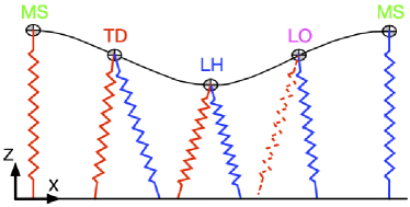
Figure 2: Sagittal plane view of nominal “human-like” CoM trajectory in a full walking step of the 3D Dual-SLIP model.

Each gait event can be associated with a gait event surface, where each event takes place when the CoM state $\left(\bm{\dot{p}}_{c},\bm{p}_{c}\right)$ crosses the corresponding surface. For a step where a leg $A$ is initially in support, the following surfaces are defined:

$$S_{MS}= \left\{\left(\bm{\dot{p}}_{c},\bm{p}_{c}\right)\big{|}\;\dot{z}_{c}=0\;,\;z_{c}>z_{TH},\|\bm{l_{A}}\|<l_{0}\right\},$$ (4)

$$S_{TD}= \left\{\left(\bm{\dot{p}}_{c},\bm{p}_{c}\right)\big{|}\;\dot{z}_{c}<0\;,\;z_{c}=z_{TH},\|\bm{l_{A}}\|\leq l_{0}\right\},$$ (5)

$$S_{LH}= \left\{\left(\bm{\dot{p}}_{c},\bm{p}_{c}\right)\big{|}\;\dot{z}_{c}=0\;,\;z_{c}<z_{TH},\|\bm{l_{A}}\|\leq l_{0}\right\},$$ (6)

$$S_{LO}= \left\{\left(\bm{\dot{p}}_{c},\bm{p}_{c}\right)\big{|}\;\dot{z}_{c}>0\;,\;\|\bm{l_{A}}\|=l_{0}\right\},$$ (7)

where $z_{TH}=l_{0}\sin{\theta}$ is the threshold CoM height at which TD takes place. More importantly, the surfaces $S_{TD}$ and $S_{LO}$ are the switching surfaces for the hybrid dynamics of the system, as they determine when the system should switch from SS to DS dynamics, and vice versa.

II-A1 Finding Periodic Gaits

As in [9], we employ a nonlinear optimization approach to obtain suitable values for the state and control variables that lead to periodic, left-right symmetric walking gaits. Now, this optimization method relies on the symmetry of the CoM about LH over one step. In the case of uneven terrain, however, that symmetry ceases to exist [10]. As a result, the half-step optimization can only be utilized for locomotion over terrains with high stiffness values.

To derive the stride map, we consider a slice of the full 3D Dual-SLIP state associated with the MS event; i.e.,

$$\bm{x}=[x_{c}-x_{f,i}\quad y_{c}-y_{f,i}\quad z_{c}\quad\dot{x}_{c}\quad\dot{y}_{c}]^{\intercal},$$ (8)

where $i\in\{A,B\}$ again denotes the leg in support. Moreover, the forward and lateral touchdown angles together with the leg stiffness value, same for both legs, will be considered as control inputs available for regulating the state evolution of the system; that is, $\bm{u}=[\theta\quad\phi\quad k]^{\intercal}$, where $k_{A}=k_{B}=k$.

Following the notation of [9], let $\bm{x}_{n}$ and $\bm{u}_{n}$ denote the values of the state and control variables at the $n$-th MS event. Then, the state at the next MS event can be computed as $\bm{x}_{n+1}=\bm{f}(\bm{x}_{n},\bm{u}_{n})$, where the map $\bm{f}$ is calculated numerically by integrating the dynamics according to the sequence of events shown in Fig. 2. Note here that the states $\bm{x}_{n}$ and $\bm{x}_{n+1}$ refer to SS phases with different legs providing support; e.g., if $\bm{x}_{n}$ refers to the $n$-th MS with leg $A$ providing support, the state $\bm{x}_{n+1}$ refers to the $(n+1)$-thMS with leg $B$ providing support. In this work, we will be concerned with nominal walking gaits that are periodic and left-right symmetric. This implies that—nominally—the states $\bm{x}_{n}$ and $\bm{x}_{n+1}$ corresponding to subsequent MS events must be related by the following symmetry condition

$$\bm{x}_{n+1}=\bm{A}\bm{x}_{n}$$ (9)

where $\bm{A}=diag(1,-1,1,1,-1)$. In words, this condition implies that in the walking gaits we consider here, the forward and vertical position and velocity remain constant from one step to the next while the lateral position and velocity alternate their sign.

To obtain suitable values for the control input and state variables that lead to a periodic left-right symmetric gait, we adopt the quarter-period (from the MS to the LH event) nonlinear optimization method suggested in [9]. In more detail, the objective of the optimization is to ensure that the projection of the CoM on the ground at the LH event lies directly between the two support feet. Assuming—without loss of generality—that leg $A$ provides support, this can be achieved by minimizing the index

$$\begin{split}&\min_{\bm{u}_{0},z_{0}}\left\{\left\|\frac{1}{2}\left(x_{f,A}+x_{f,B}\left(\bm{x_{0}},\bm{u_{0}}\right)\right)-x_{c}\left(t_{LH};\bm{x_{0}},\bm{u_{0}}\right)\right\|^{2}\right.\\ &+\left.\left\|\frac{1}{2}\left(y_{f,A}+y_{f,B}\left(\bm{x_{0}},\bm{u_{0}}\right)\right)-y_{c}\left(t_{LH};\bm{x_{0}},\bm{u_{0}}\right)\right\|^{2}\right\},\end{split}$$ (10)

subject to the dynamics of the system initiated at MS; in (10), $t_{LH}$ is the time instance where the first LH takes place and $\bm{x_{0}}$, $\bm{u_{0}}$ denote the initial MS state and control input variables, respectively. As in [9], we restrict the optimization search for $\bm{x_{0}}$ to the following family of states

$$\begin{split}\bm{x}_{0}&=[x_{0,d}\quad y_{0,d}\quad z_{0}\quad\dot{x}_{0,d}\quad\dot{y}_{0,d}]\\ x_{0,d}&=0\;m,\;y_{0,d}=0.05\;m,\;\dot{y}_{0,d}=0\;m/s\end{split}$$ (11)

where $\dot{y}_{0,d}=0\;m/s$ is needed to satisfy the periodic gait conditions in [9, Equation (9)] and for a rest leg length $l_{0}=1\;m$, we set $y_{0,d}=0.05\;m$, similar to [9]. Regarding the remaining two state variables, the forward velocity $\dot{x}_{0,d}$ at MS is specified by the user and the height $z_{0}$ is a decision variable. The optimizer then selects values for $z_{0}$ and the input variables $\bm{u}_{0}$ to minimize the cost function (10).

In this work, we first implemented the proposed method for the regular 3D Dual-SLIP, using a forward velocity of 1 $m/s$, $m=80\;kg$, $l_{0}=1\;m$, and derived the following optimal set of parameters using the nonlinear least-squares function lsqnonlin in Matlab^TM:

$$\begin{split}\bm{x}_{0}&=[x_{0,d}\quad y_{0,d}\quad z_{0}\quad\dot{x}_{0,d}\quad\dot{y}_{0,d}]\\ &=[0\;m\quad 0.05\;m\quad 0.99\;m\quad 1\;m/s\quad 0\;m/s],\end{split}$$ (12)

$$\begin{split}\bm{u}_{0}&=[\theta_{0}\quad\phi_{0}\quad k_{0}]^{\intercal}\\ &=[107.26^{\circ}\quad 10.94^{\circ}\quad 14163.54\;N/m].\end{split}$$ (13)

II-A2 The LQR Controller

Let $\bm{x}_{0}^{*},\bm{u}_{0}^{*}$ be an optimal set of parameters resulting in a left-right symmetric gait for a specific forward velocity. Along this gait, the MS states evolve according to (9) so that the nominal $n$-th MS state is given by $\bm{x}_{n}^{*}=\bm{A}^{n}\bm{x}_{0}^{*}$ under the condition that the control parameters are selected according to $\bm{u}_{n}^{*}=\bm{B}^{n}\bm{u}_{0}^{*}$ with $\bm{B}=diag(-1,1,1)$ to account for the sign-alternating forward touchdown angle at each step. Under non-nominal conditions, however, initiating the system with $\bm{x}_{0}^{*},\bm{u}_{0}^{*}$ will not result in periodic locomotion due to the presence of disturbances. Thus, if $\bm{x}_{n}$ denotes the actual value of state at the $n$-th MS event, we have $\bm{x}_{n}\neq\bm{x}_{n}^{*}$. To ensure that the actual MS state $\bm{x}_{n}$ approaches the nominal periodic evolution $\bm{x}_{n}^{*}$, a discrete-time, infinite-horizon LQR will be designed; the procedure closely follows [9], and thus our exposition here will be terse.

Let $\Delta\bm{x}_{n}=(\bm{x}_{n}-\bm{x}_{n}^{*})$, $\Delta\bm{u}_{n}=(\bm{u}_{n}-\bm{u}_{n}^{*})$, $\Delta\tilde{\bm{x}}_{n}=\bm{A}^{n}\Delta\bm{x}_{n}$, $\Delta\tilde{\bm{u}}_{n}=\bm{B}^{n}\Delta\bm{u}_{n}$. In [9], it is shown that

$$\Delta\tilde{\bm{x}}_{n+1}\approx\bm{J}_{x}\Delta\tilde{\bm{x}}_{n}+\bm{J}_{u}\Delta\tilde{\bm{u}}_{n},$$ (14)

where $\bm{J}_{x}=\bm{A}\frac{\delta\bm{f}}{\delta\bm{x}}$ and $\bm{J}_{u}=\bm{A}\frac{\delta\bm{f}}{\delta\bm{u}}$ are evaluated at $(\bm{x}_{0}^{*},\bm{u}_{0}^{*})$. Now, consider the following quadratic cost for positive definite matrices $\bm{Q}$ and $\bm{R}$:

$$\min_{\Delta\tilde{\bm{u}}}\sum_{n=0}^{\infty}\Delta\tilde{\bm{x}}_{n}^{T}\bm{Q}\Delta\tilde{\bm{x}}_{n}+\Delta\tilde{\bm{u}}_{n}^{T}\bm{R}\Delta\tilde{\bm{u}}_{n}$$ (15)

$$\text{s.t. }\Delta\tilde{\bm{x}}_{n+1}=\bm{J}_{x}\Delta\tilde{\bm{x}}_{n}+\bm{J}_{u}\Delta\tilde{\bm{u}}_{n}.$$ (16)

Then, if $\left(\bm{J}_{x},\bm{J}_{u}\right)$ is controllable, the following time-invariant feedback gain is obtained:

$$\bm{K}=-(\bm{J}_{u}^{T}\bm{P}\bm{J}_{u}+\bm{R})^{-1}\bm{J}_{u}^{T}\bm{P}\bm{J}_{x},$$ (17)

where $\bm{P}$ is the unique solution of the Discrete-Time Algebraic Riccati Equation (DARE). This results in the following time-invariant control law

$$\bm{u}_{n}=\bm{u}_{n}^{*}+\bm{B}^{n}\bm{K}\bm{A}^{n}(\bm{x}_{n}-\bm{x}_{n}^{*})$$ (18)

which adjusts the control input at each MS event to regulate the state so that it converges to the target periodic gait. Note that in this work, we will refer to a controller obtained for $\bm{Q}=\bm{R}=\bm{I}$, where $\bm{I}$ is the identity matrix, as an identity LQR controller.

In order to verify the validity of the modified dynamics that account for the compliance of the terrain, locomotion over high stiffness values was tested to simulate rigid terrain walking. After running multiple simulations with different stiffness values, it was concluded that a stiffness of $k_{g,A}=k_{g,B}=50\;MN/m$ resulted in a response closest to the one observed for the ideal rigid case, described in previous works [9, 16]. Specifically, the system was able to reach at least 100 steps, which can be interpreted as a sign of stable performance and hence successful implementation of the proposed methodology [8]. Therefore, the stiffness of $50\;MN/m$ will be considered from now on as the equivalent of the rigid terrain, meaning that any terrain with a stiffness lower than that will be considered as compliant. In the aforementioned simulations, the system was simulated using $m=80\;kg$, $l_{0}=1\;m$, and $m_{f,A/B}=1\;kg$, while the same optimal initial conditions and identity LQR controller were utilized, as the ones analyzed in Sections II-A1 and II-A2.

II-B One-step Unilateral Low Stiffness Perturbations

As a first step towards achieving periodic gait over compliant terrains, we investigate the response of the model to one-step unilateral low stiffness perturbations. For these simulations, the model was initiated using a set of optimal parameters to achieve periodic gait, while the ground stiffness was set to the rigid value of $50\;MN/m$. Then, after $n_{p}$ steps the system experienced a one-step unilateral lower stiffness perturbation, after which the ground stiffness was set back to rigid as depicted in Fig. 3. Specifically, during the $n_{p}$ step the ground stiffness under the leg about to land ($A$) was lowered to a specific value at TD and was kept constant throughout the whole stance phase of that leg (TD to LO). Then, the ground stiffness was reset to rigid for the rest of the trial. The ground stiffness of the other leg ($B$) remained fixed to rigid throughout the whole trial. It should be noted that such perturbations have been applied to humans before for understanding human gait and for rehabilitation purposes using a novel instrumented device [18, 19, 20].

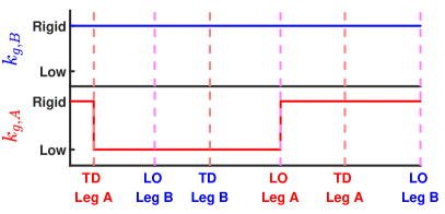
Figure 3: Timing of the one-step unilateral low stiffness perturbation. Top and bottom figures illustrate the ground stiffness values underneath the legs $B$ and $A$, respectively. Rigid ground stiffness corresponds to $50\;MN/m$, while low ground stiffness can take any value lower than that. The color of the label for each gait event indicates the related leg (blue for leg $B$, red for leg $A$).

II-C Biomechanics-inspired Proposed Controller

Inspired by human locomotion, we propose a modified controller for the 3D Dual-SLIP, which adjusts the stiffness of the legs in support, to withstand one-step unilateral low stiffness perturbations. Previously, Ferris et al. showed that runners increased leg stiffness for their first step when transitioning from hard to softer surfaces [15]. As the runners were expecting the perturbation, they tended to pre-adjust the increased leg stiffness during their last step on the hard surface. Inspired by this, we propose a controller that increases the leg stiffness of both legs of the 3D Dual-SLIP to handle expected one-step unilateral low stiffness perturbations.

The proposed feedback law is based on the LQR controller developed in Section II-A2, modified to allow for further stiffening of the legs when needed; an overview of the proposed controller is illustrated in Fig. 4. In more detail, initially both legs share the same stiffness value, as determined by the LQR controller at each step $n$; i.e., $k_{A}=k_{B}=k_{n}$. Then, at the TD event of the perturbation step ($n_{p}$), the stiffness of the leg about to land is increased to $k_{A}=k_{1}k_{n_{p}}$, where $k_{1}>1$ is a control gain and $k_{n_{p}}$ is the stiffness value derived by the LQR controller for that step. At the same time, the stiffness of the leg in support is also increased to $k_{B}=k_{2}k_{n_{p}}$, where $k_{2}>1$ is again a control gain. These stiffness values remain constant as long as each leg is in stance phase. At the MS event of the following step ($n_{p}+1$), the stiffness of the leg experiencing the perturbation, retains the same control gain $k_{A}=k_{1}k_{n_{p}+1}$, while the stiffness of the leg about to land on rigid terrain is set back to $k_{B}=k_{n_{p}+1}$. Finally, by the time the next MS event takes place, the leg that experienced the perturbation has switched to swing phase (LO) and is about to land on rigid terrain. Therefore, from that point on, both legs share again the same stiffness value $k_{n}$, as it is calculated by the LQR controller at each step.

Figure 4: Overview of the biomechanics-inspired proposed controller. The model is initiated with the optimal state-control pair ($\bm{x_{0}^{*}},\bm{u_{0}^{*}}$) to achieve periodic gait with a desired forward velocity at MS. The {MS, TD} and {LH, LO} gait events are identified using single support (SS) and double support (DS) dynamics, respectively. At every MS event, the LQR controller is implemented and the $\bm{u_{n}}$ feedback law is derived. During the perturbation step ($n=n_{p}$), the stiffness of both legs is initially determined by the LQR controller at MS (Q1) and then it is amplified at TD by the control gains $k_{1}$ and $k_{2}$ (Q2). At the next step ($n=n_{p}+1$), the leg experiencing the perturbation ($A$) maintains an increased stiffness at MS, while the stiffness of the leg about to land on rigid terrain ($B$) is determined based on the LQR controller with no adjustment (Q3). Then, at TD, the stiffness of both legs is not altered (Q4). Finally, the stiffness for both legs is determined based on the LQR for all other steps.

III Results

In this section, the proposed controller will be compared to the standard LQR controller designed for rigid surfaces, with respect to their response to unilateral one-step low stiffness perturbations. For all simulations, the model parameters mentioned in the Methods Section were used and the model was initiated with the optimal set of parameters ($\bm{x_{0}^{*}},\bm{u_{0}^{*}}$) shown in (12)-(13). For all one-step unilateral low stiffness perturbations, the perturbation took place at the tenth step ($n_{p}=10$). All simulations were implemented and executed in MATLAB^TM version 9.7 (R2019b), where the nonlinear least-squares function lsqnonlin and the embedded fixed-step integrator ode4 were utilized for the optimization and the dynamic simulation, respectively.

III-A Performance of the Standard LQR Controller

Initially, the robustness of the standard LQR controller was explored under one-step unilateral perturbations of various ground stiffness levels. In all simulations, an identity LQR controller was used. For perturbation ground stiffness values ranging from 50 $MN/m$ to 200 $kN/m$, the system was shown to be able to endure the one-step perturbation and reach the threshold performance of 100 steps. Four representative cases are shown in Fig. 5 for ground stiffness values of $50\;MN/m$, $1\;MN/m$, $500\;kN/m$ and $200\;kN/m$. It should be noted that in all four cases the model was able to achieve the desired number of 100 steps, but for brevity we chose to show the system response only for up to the $25^{th}$ step. As it can be observed, the perturbation introduces errors in all state variables, the magnitude of which increases as the perturbation stiffness decreases. Nevertheless, the LQR controller is able to regulate the introduced errors and lead the system to steady-state for all cases. Although the error is minimized in less than 10 steps, small steady-state errors are evident for some state variables, which again increase as the perturbation stiffness decreases.

For ground stiffness values lower than 200 $kN/m$, the perturbation destabilized the system and caused it to fail, i.e. the system was not able to complete a proper step after the perturbation. Considering the stiffness levels reported in [6], the 200 $kN/m$ stiffness level would be classified as moderate ground. As a result, it appears that the standard LQR controller proposed for locomotion over rigid terrain is able to handle one-step unilateral low stiffness perturbations, only up to moderate ground stiffness values.

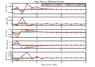
Figure 5: State error response for stiffness perturbations of 50 $MN/m$, 1 $MN/m$, 500 $kN/m$ and 200 $kN/m$ using the standard LQR controller.

III-B Performance of the Proposed Controller

As an extension of the standard LQR controller, the proposed controller inherits its stable performance for perturbation ground stiffness values ranging from 50 $MN/m$ to 200 $kN/m$. Therefore, we focus only on stiffness values lower than the 200 $kN/m$ threshold. Again, identity $\bm{Q}$ and $\bm{R}$ matrices were utilized for the LQR part of the proposed controller. For stiffness values lower than 200 $kN/m$, we showed that the system with the proposed controller is able to endure perturbations of stiffness as low as 30 $kN/m$. It should be noted that this stiffness value is much lower than the soft ground category of 80 $kN/m$ reported in [6], and it resembles walking on a foam pad [21]. Four representative cases are shown for one-step perturbations of 200, 150, 90 and 30 $kN/m$ in Fig. 6. Similarly to Fig. 5, we chose to show the system response only up to the $25^{th}$ step, although the desired number of 100 steps was achieved for all cases.

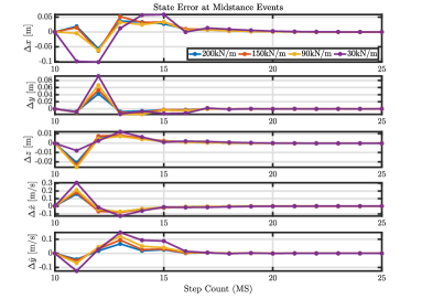
Figure 6: State error response for stiffness perturbations of 200, 150, 90 and 30$\;kN/m$ using the proposed controller.

Similar to the higher stiffness levels shown in Fig. 5, the perturbations again introduce errors, the magnitude of which increases as the ground stiffness decreases. As it can be seen in all cases, the model manages to handle the perturbation taking place at the $10^{th}$ step, while the proposed controller regulates any introduced errors and leads to zero steady-state errors. The rapid recovery of the system is to be noted, as the error is suppressed in less than 10 steps. Moreover, by comparing the responses of the model for the 200 $kN/m$ perturbation between the standard and the proposed controller, it is clear that the proposed controller leads to smaller errors during both the transient and the steady-state response. For all four perturbation stiffness values, the control gains ($k_{1},k_{2}$) were tuned to minimize the steady-state errors. The control gains used are listed in Table I, where it can be seen that as the perturbation stiffness decreases, higher control gains have to be used to handle the perturbation and achieve zero steady-state errors.

Figure 7 shows the model experiencing a stiffness perturbation of 200 $kN/m$, while a video demonstration of the 3D Dual-SLIP experiencing one-step unilateral stiffness perturbations in simulation can be found at [22]. Before the perturbation, the stiffness of the legs is set based on the internal LQR controller. At the TD event during the perturbation step, the stiffness of the legs is amplified throughout each leg’s stance phase. Then, during the perturbation, the perturbed leg reaches the maximum foot penetration depth, maintaining the amplified stiffness, while the stiffness for the unperturbed leg is again set based on the LQR controller. Finally, after the perturbation, both legs share again the same stiffness, as calculated by the LQR controller.

In order to highlight the significance and the physical meaning of the perturbations, the maximum penetration depth of the foot stepping on the soft surface is provided in Table I for all four cases. As expected, lower perturbation stiffness values correspond to deeper penetration depths. More importantly, given that the leg rest length is 1 $m$, the model manages to regulate an extensive vertical sinking of the perturbed leg, close to 12% of the leg’s rest length, in the case of the lowest stiffness of 30 $kN/m$.

Perturbation Stiffness (kN/m)		200	150	90	30
Control Gains	$k_{1}$	1.05	1.1	1.4	8.4
	$k_{2}$	1.14	1.19	1.36	3.17
Max Penetration Depth (cm)		2.65	3.21	4.64	11.49

TABLE I: Control gains and maximum penetration depth for one-step unilateral stiffness perturbations using the proposed controller.

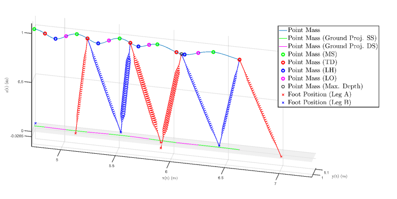
Figure 7: The 3D Dual-SLIP model experiencing an one-step unilateral stiffness perturbation of 200 $kN/m$. Blue line on top illustrates the three dimensional trajectory of the CoM, while the green and magenta lines on the bottom denote its projection on the x-y plane, during the SS and DS phases, respectively. Green, red, blue and magenta circles ($\circ$) represent the position of the CoM during the MS, TD, LH and LO gait events, respectively. Black circle indicates the position of the CoM when the perturbed foot reaches the maximum penetration depth (0.0265 $m$). Red and blue crosses ($\times$) depict the position of the feet for legs $A$ and $B$, respectively. The increased coil radius of the spring legs in the second and third snapshot of the model indicates an increase in leg stiffness due to the proposed controller.

IV Conclusion

This paper extends the 3D Dual-SLIP model to support for the first time locomotion over compliant terrains and proposes a novel biomechanics-inspired controller to regulate one-step unilateral low stiffness perturbations. Using a standard LQR controller, the extended model is shown to be able to endure such perturbations only up to a moderate ground stiffness level of 200 $kN/m$. On the contrary, the proposed controller can produce stable gait at stiffness levels as low as 30 $kN/m$, which results in vertical sinking of the $1m$-long leg as deep as 11.49 $cm$. Therefore, the proposed controller allows for robust dynamic walking over extremely low stiffness one-step unilateral perturbations. As robust and stable walking over a wide range of compliant terrains is an important problem for legged locomotion, this work can significantly advance the field of bipedal walking by improving the control of bipeds and humanoids, as well as prosthetic devices with tunable stiffness.

References

- [1] M. M. Venâncio, R. S. Gonçalves, and R. A. d. C. Bianchi, “Terrain identification for humanoid robots applying convolutional neural networks,” IEEE/ASME Transactions on Mechatronics, vol. 26, no. 3, pp. 1433–1444, 2021.
- [2] M. Wang, M. Wonsick, X. Long, and T. Padr, “In-situ terrain classification and estimation for nasa’s humanoid robot valkyrie,” in 2020 IEEE/ASME International Conference on Advanced Intelligent Mechatronics (AIM), 2020, pp. 765–770.
- [3] G. Mesesan, J. Englsberger, G. Garofalo, C. Ott, and A. Albu-Schäffer, “Dynamic walking on compliant and uneven terrain using dcm and passivity-based whole-body control,” in 2019 IEEE-RAS 19th International Conference on Humanoid Robots (Humanoids), 2019, pp. 25–32.
- [4] M. A. Hopkins, A. Leonessa, B. Y. Lattimer, and D. W. Hong, “Optimization-based whole-body control of a series elastic humanoid robot,” International Journal of Humanoid Robotics, vol. 13, no. 01, p. 1550034, 2016.
- [5] R. J. Full and D. E. Koditschek, “Templates and anchors: neuromechanical hypotheses of legged locomotion on land,” Journal of experimental biology, vol. 202, no. 23, pp. 3325–3332, 1999.
- [6] V. Vasilopoulos, I. S. Paraskevas, and E. G. Papadopoulos, “Compliant terrain legged locomotion using a viscoplastic approach,” in 2014 IEEE/RSJ International Conference on Intelligent Robots and Systems, 2014, pp. 4849–4854.
- [7] I. Poulakakis and J. W. Grizzle, “The spring loaded inverted pendulum as the hybrid zero dynamics of an asymmetric hopper,” IEEE Transactions on Automatic Control, vol. 54, no. 8, pp. 1779–1793, 2009.
- [8] H. Geyer, A. Seyfarth, and R. Blickhan, “Compliant leg behaviour explains basic dynamics of walking and running,” Proceedings of the Royal Society B: Biological Sciences, vol. 273, no. 1603, pp. 2861–2867, 2006.
- [9] Y. Liu, P. M. Wensing, D. E. Orin, and Y. F. Zheng, “Dynamic walking in a humanoid robot based on a 3d actuated dual-slip model,” in 2015 IEEE International Conference on Robotics and Automation (ICRA), 2015, pp. 5710–5717.
- [10] Y. Liu, P. M. Wensing, D. E. Orin, and Y. F. Zheng, “Trajectory generation for dynamic walking in a humanoid over uneven terrain using a 3d-actuated dual-slip model,” in 2015 IEEE/RSJ International Conference on Intelligent Robots and Systems (IROS), 2015, pp. 374–380.
- [11] X. Xiong and A. Ames, “Slip walking over rough terrain via h-lip stepping and backstepping-barrier function inspired quadratic program,” IEEE Robotics and Automation Letters, vol. 6, no. 2, pp. 2122–2129, 2021.
- [12] L. C. Visser, S. Stramigioli, and R. Carloni, “Robust bipedal walking with variable leg stiffness,” in 2012 4th IEEE RAS EMBS International Conference on Biomedical Robotics and Biomechatronics (BioRob), 2012, pp. 1626–1631.
- [13] X. Liu, A. Rossi, and I. Poulakakis, “A switchable parallel elastic actuator and its application to leg design for running robots,” IEEE/ASME Transactions on Mechatronics, vol. 23, no. 6, pp. 2681–2692, 2018.
- [14] D. P. Ferris, M. Louie, and C. T. Farley, “Running in the real world: adjusting leg stiffness for different surfaces,” Proceedings of the Royal Society of London. Series B: Biological Sciences, vol. 265, no. 1400, pp. 989–994, 1998.
- [15] D. P. Ferris, K. Liang, and C. T. Farley, “Runners adjust leg stiffness for their first step on a new running surface,” Journal of biomechanics, vol. 32, no. 8, pp. 787–794, 1999.
- [16] Y. Liu, A Dual-SLIP Model For Dynamic Walking In A Humanoid Over Uneven Terrain. The Ohio State University, 2015.
- [17] W. J. Stronge, Impact mechanics. Cambridge university press, 2018.
- [18] J. Skidmore and P. Artemiadis, “Unilateral walking surface stiffness perturbations evoke brain responses: Toward bilaterally informed robot-assisted gait rehabilitation,” in 2016 IEEE International Conference on Robotics and Automation (ICRA), 2016, pp. 3698–3703.
- [19] J. Skidmore, A. Barkan, and P. Artemiadis, “Investigation of contralateral leg response to unilateral stiffness perturbations using a novel device,” in 2014 IEEE/RSJ International Conference on Intelligent Robots and Systems, 2014, pp. 2081–2086.
- [20] J. Skidmore, A. Barkan, and P. Artemiadis, “Variable stiffness treadmill (VST): System development, characterization, and preliminary experiments,” IEEE/ASME Transactions on Mechatronics, vol. 20, no. 4, pp. 1717–1724, 2014.
- [21] W. Bosworth, J. Whitney, S. Kim, and N. Hogan, “Robot locomotion on hard and soft ground: Measuring stability and ground properties in-situ,” in 2016 IEEE International Conference on Robotics and Automation (ICRA), 2016, pp. 3582–3589.
- [22] https://youtu.be/xKRRyGAfvzs.