Recovering information in an asymptotically flat spacetime in quantum gravity

Abstract

As an extension of arXiv:{2002.02448, 2008.10740} we present a physical protocol that a set of observers can use to detect a pure state in the bulk when they are spread across a small cut near ${\cal I}^{+}_{-}$ in flat spacetime. The protocol involves the modification of a bulk state using simple unitary operators and measurements of the energy of the state. The states that we study are constructed by acting with low energy operators on a vacuum state such that a perturbative analysis is valid. We restrict ourselves to $3+1$ dimensional spacetimes and only consider massless excitations. From this analysis, the principle of holography of information becomes manifest in the case of asymptotically flat spacetime.

1 Introduction and Setup

In [Chowdhury:2020hse] it was shown that a set of observers living on a thin time band in global Anti-de Sitter space (AdS) can determine a state in the bulk via a physical protocol in a theory of quantum gravity. The existence of such a protocol is a consequence of the principle of holography of information, which was established in a series of papers [Laddha:2020kvp, Raju:2019qjq, Chowdhury:2021nxw] and is reviewed in [Raju:2020smc]. For a theory of quantum gravity in flat spacetime, this states that all information about a state in the bulk is also available at a small cut near the past of the future null infinity ${\cal I}^{+}_{-}$ (or near the future of past null infinity ${\cal I}^{-}_{+}$). The validity of the principle relies on the following basic properties of semi-classical gravity as elucidated by DeWitt [DeWitt:1967yk] and later expanded in [Laddha:2020kvp, Raju:2019qjq, Chowdhury:2021nxw]:

1. Any finite energy excitation in the bulk must leave an imprint at the boundary due to the uncertainty principle. As a corollary, this also implies that there are no local gauge invariant operators in gravity.

2. The Hamiltonian of the theory is a boundary term and can be expressed in terms of the metric fluctuations at the boundary (eg: see equation (3.1)).

3. We assume that the Hamiltonian (3.1) remains positive in the quantum theory as it is quadratic in the degrees of freedom.

4. The eigenstate of the Hamiltonian with the least energy is defined to be the vacuum state and its energy is renormalized to zero.

We will require these properties to hold in perturbative gravity and will be using them throughout the paper.

The best known example of the principle of holography of information is the AdS/CFT correspondence [adscft, Witten:1998qj]. However the authors of [Laddha:2020kvp] demonstrated how the principle works in $3+1$ dimensional flat spacetime with gravity coupled to massless matter. They showed that all information on a Cauchy slice in the bulk is also available at ${\cal I}^{+}_{-}$ (or ${\cal I}^{-}_{+}$). Motivated by this, we follow a similar program as in [Chowdhury:2020hse] and establish a physical protocol for detecting a certain class of excitations in $3+1$ dimensional flat spacetime in a theory of gravity coupled to massless matter fields.

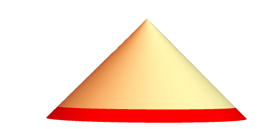
Figure 1: Location of observers near ${\cal I}^{+}_{-}$ in Flat spacetime. The state $\ket{\psi}$ is composed of operators spread across all of ${\cal I}^{+}$ (denoted by the yellow + red region of the cone) but the measurements are only performed in the red region.

The observers are localized in a small region near ${\cal I}^{+}_{-}$ as depicted by the red band in figure(1). They are given the task of determining a state $\ket{\psi}$ by performing certain measurements. These include the measurement of conserved charges (localized at ${\cal I}^{+}_{-}$) and also a modification of the state $\ket{\psi}$ by unitary operators near ${\cal I}^{+}_{-}$. The latter restriction is necessary because in any physical process the observers can modify the interaction Hamiltonian (between themselves and the system) by Hermitian operators. In perturbation theory, this results in the action of a unitary operator acting on the state.

It has been shown [Laddha:2020kvp] that the knowledge of all possible correlation functions composed of operators near ${\cal I}^{+}_{-}$, in a particular state, allows one to reconstruct the state itself. However in this paper we are restricting ourselves to measurements which can be performed by observers localized at ${\cal I}^{+}_{-}$ in a “physical experiment”. For this purpose we shall only consider a class of states $\ket{\psi}$ which are built by exciting the vacuum state $\ket{0}$ by low energy operators. There are more general classes of states as discussed in [Marolf:2015jha] but the examination of these and a construction of a protocol to detect them from ${\cal I}^{+}_{-}$ are left for future work.

We now discuss the difficulties in constructing such a protocol in flat spacetime as compared to AdS. Flat spacetime has an intricate IR structure due to the presence of an infinite dimensional symmetry [He:2014laa, Strominger:2014pwa, Strominger:2017zoo] which leads to an infinitely degenerate vacuum state. Thus flat spacetime has multiple vacua in contrast to the AdS spacetime that has a unique vacuum.

Another major difficulty in flat spacetime is the lack of a discrete energy spectrum (as is the case for the AdS spacetime). Since the energy is continuous in flat spacetime it is not useful to decompose a state $\ket{\psi}$ in terms of a basis spanned by energy eigenstates. However, we can still exploit the fact that there is a lower bound of the energy when measured from asymptotic infinity, which we renormalize to zero. Subsequently, we introduce a more convenient basis to decompose the states. This is called the normal-ordered basis, which is very similar to the usual Fock basis (see eq. (3.1)). Throughout this paper we represent the matter fields with scalars but this restriction can be relaxed and we can consider fields of any spin (or even stringy excitations). By causality, any massless excitation can be expressed in terms of operators smeared over ${\cal I}^{+}$ and therefore the basis is constructed out of fields living at ${\cal I}^{+}$. A similar basis construction is also possible in AdS spacetime but in that case it was more convenient to work with an energy eigen basis [Chowdhury:2020hse].

In this paper we shall restrict to measuring the energy of states built using hard operators (an operator with finite energy) on a particular vacuum state denoted by $\ket{0}$. Using the Born-rule, this reduces to computing expectation values of a product of unitary operators and the projector onto the vacuum state. We will show that this allows us to completely decode a state of the kind shown in eq.(3.1).

As discussed below, such a protocol does not violate causality. This is because, in order to measure the energy of a state, the observers are forced to be spread over the whole Celestial sphere since the energy is expressed as a surface integral of metric fluctuations over the entire Celestial sphere (see equation (3.1)). Hence each observer only measures a part of the metric fluctuation and in order to evaluate the energy, they have to meet and sum their results. This process clearly takes more than the light crossing time and therefore prevents any violation of causality.

We end this section by stating why such a protocol only works in a theory of gravity and not in other gauge theories or Local QFTs (LQFT). In an ordinary LQFT (without dynamical gravity) such a protocol would clearly fail since there exists operators which commute with all operators at ${\cal I}^{+}_{-}$ because of micro-causality. Therefore it is not possible to distinguish a state $\ket{\psi}$ from the state $U_{bulk}\ket{\psi}$ where $U_{bulk}$ is any unitary operator in the bulk. Similar local operators also exist in a gauge theory (example: in QED we have $F_{\mu\nu}^{2}$) which prevent the reconstruction of information in those theories. This counter argument does not work in quantum gravity as the notion of micro-causality relies on spacelike separation and since the metric itself fluctuates at $O(\sqrt{G_{N}})$ [Arkani-Hamed:2007ryv, Donnelly:2015hta] in a theory of quantum gravity, micro-causality is violated perturbatively in $O(\sqrt{G_{N}})$. Even though this is a tiny violation, it can be observed in the regime of effective field theory and this will become apparent in the main text.

We review the Hilbert space structure of flat spacetime in section 2, then properly define the main question and its solution in section 3 and end with conclusions and discussions on various related ideas in section LABEL:discussion.

2 Hilbert Space of Flat Spacetime

In this section we review the asymptotic structure of Minkowski spacetime and how its information is encoded in data at null infinity [Laddha:2020kvp, Ashtekar:1981sf, Ashtekar:1987tt]. Moreover, we will revisit how upon quantization these data give rise to the Hilbert space of the low energy effective theory.

The metric for an asymptotically flat space time near ${\cal I}^{+}$ can be written in the retarded Bondi coordinates [Bondi:1962px, Sachs:1962wk] as

$$ds^{2}=-du^{2}-2dudr+r^{2}\gamma_{AB}d\Omega^{A}d\Omega^{B}+rC_{AB}d\Omega^{A}d\Omega^{B}+\frac{2m_{B}}{r}du^{2}+\gamma^{AC}D_{C}C_{AB}dud\Omega^{B}+...\,,$$ (2.1)

where the retarded time $u=t-r$ with $t$ being the time, $r$ the radial direction and $\Omega=(\theta,\phi)$ the coordinates on the unit sphere $S^{2}$. The capital latin letters $A,\cdots$ take values on the unit sphere and $\gamma_{AB}$ is the metric of the unit $S^{2}$. $C_{AB}(u,\Omega)$ is the shear field and it encodes the information about the radiative degrees of freedom. In this gauge $\gamma^{AB}C_{AB}=0$, thus the shear is traceless. The radiative data are encoded at future null infinity $\mathcal{I}^{+}$ which has the topology $\mathbb{R}\times S^{2}$ and is parametrized by $(u,\Omega)$. The afforementioned unit $S^{2}$ is called the Celestial sphere. $D_{A}$ is the covariant derivative with respect to the metric $\gamma_{AB}$ and $m_{B}$ is the Bondi mass aspect.

Throughout this paper we shall work with matter fields which are massless scalar fields, however the results are easily generalizable to other massless fields. The large$-r$ fall-off of the scalar field is fixed by demanding the finiteness of its energy

$$\lim_{r\to\infty}\phi^{bulk}(u,r,\Omega)=\frac{1}{r}\phi(u,\Omega)+\mathcal{O}\Big{(}\frac{1}{r^{2}}\Big{)}\,,$$ (2.2)

where $\phi(u,\Omega)$ encodes the classical radiative data of the matter field.

At null infinity the gravitational and matter data are not independent as they are related by the Hamiltonian constraint of General relativity. This can be explicitly seen from the $uu$-component of the Einstein equation which gives the evolution equation for the Bondi mass aspect

$$\partial_{u}m_{B}=\frac{1}{4}D^{A}D^{B}N_{AB}-\frac{1}{8}N_{AB}N^{AB}-4\pi GT_{uu}^{(0)}\,,$$ (2.3)

where $N_{AB}=\partial_{u}C_{AB}$ is the Bondi News tensor and $T_{uu}^{(0)}$ is the leading order of the matter stress tensor, which for a scalar field is given by $\frac{1}{2}(\partial_{u}\phi)^{2}$. Thus $m_{B}$ is a function of the radiative data and of an integration constant at $u=-\infty$ (the Bondi mass at ${\cal I}^{+}_{+}$ is zero since we do not consider massive particles here).

We move forward to introduce the phase space and the conserved charges. The radiative phase space is characterized in terms of the News and the Shear tensor. The Poisson brakets between the two was found to be [Ashtekar:1981sf, Ashtekar:1987tt, Ashtekar:1981bq]

$$\left\{N_{AB}(u,\Omega),C_{MN}(u^{\prime},\Omega^{\prime})\right\}=-\frac{16\pi}{\sqrt{\gamma}}\delta(u-u^{\prime})\delta^{2}(\Omega-\Omega^{\prime})\left[\gamma_{A(M}\gamma_{N)B}-\frac{1}{2}\gamma_{AB}\gamma_{MN}\right]\,.$$ (2.4)

This will be later promoted to a commutator upon quantizataion.

In the absence of massive particles, the conserved charges of the theory can be expressed in terms of the integration constant of $m_{B}$ at $u\to-\infty$. These charges are known as the supertranslation charge

$$\mathcal{Q}_{l,m}=\frac{1}{4\pi G_{N}}\int\sqrt{\gamma}d^{2}\Omega\ Y_{l,m}(\Omega)m_{B}(u=-\infty,\Omega)$$ (2.5)

where $Y_{l,m}$ are the spherical harmonics on $S^{2}$. $\mathcal{Q}_{l=0,m=0}$ is the familiar ADM Hamiltonian. The supertranslation charges can be separated into a soft and a hard part by using eq.(2.3). This decomposition can also be thought of as a separation into terms involving linear and non-linear News

$$\mathcal{Q}^{soft}_{l,m}=-\frac{1}{16\pi G_{N}}\int_{-\infty}^{\infty}du\,d^{2}\Omega\,\sqrt{\gamma}Y_{lm}(\Omega)\left(D^{A}D^{B}N_{AB}\right)\,,$$ (2.6a)

$$\mathcal{Q}^{hard}_{l,m}=\frac{1}{16\pi G_{N}}\int_{-\infty}^{\infty}du\,d^{2}\Omega\,\sqrt{\gamma}Y_{lm}(\Omega)\left(\frac{1}{2}N_{AB}N^{AB}+16\pi G_{N}T^{M(0)}_{uu}\right)\,.$$ (2.6b)

The action of the supertranslation generator on the radiative data at $\mathcal{I}^{+}$ is given by the following poisson brackets

$$\left\{C_{MN}(u,\Omega),\mathcal{Q}_{lm}\right\}=Y_{lm}(\Omega)\partial_{u}C_{MN}(u,\Omega)-2\Big{(}D_{M}D_{N}Y_{lm}(\Omega)-\frac{1}{2}\gamma_{MN}D^{2}Y_{lm}(\Omega)\Big{)}\,.$$ (2.7)

The radiative phase space of asymptotically flat spacetimes at future null infinity is given by free fields even at the non-linear level and the quantization of such a theory was developed by Ashetakar, et. al [Ashtekar:1981sf, Ashtekar:1987tt, Ashtekar:1981bq]. In the quantum theory one derives the following commutation relations (obtained by promoting the Poisson brackets above to commutators)

$$\left[N_{AB}(u,\Omega),N_{CD}(u^{\prime},\Omega^{\prime})\right]=16\pi iG_{N}\frac{1}{\sqrt{\gamma}}\partial_{u}\delta(u-u^{\prime})\delta^{2}(\Omega-\Omega^{\prime})\left(\gamma_{A(C}\gamma_{D)B}-\frac{1}{2}\gamma_{AB}\gamma_{CD}\right)\,,$$

$$\left[C_{AB}(u,\Omega),N_{CD}(u^{\prime},\Omega^{\prime})\right]=-8\pi iG_{N}\frac{1}{\sqrt{\gamma}}\text{sign}(u-u^{\prime})\delta^{2}(\Omega-\Omega^{\prime})\left(\gamma_{A(C}\gamma_{D)B}-\frac{1}{2}\gamma_{AB}\gamma_{CD}\right)\,,$$

where the tensors $C_{AB}$, $N_{AB}$ have been promoted to operators.

2.1 Hilbert Space

The naive Hilbert space construction leads to states with divergent norms [Ashtekar:1987tt], but as we will present below (we refer the reader to section 2.3 of [Laddha:2020kvp] for an extensive discussion) this can be resolved by defining the Hilbert space as a direct sum over Fock spaces. Each such Fock space is built on top of a specific vacuum defined by the soft part of the supertranslation charges.

The vacuum is specified by the eigenvalue of the supertranslation charge with $l>0$, i.e, the zero mode of the News

$$\mathcal{Q}_{lm}\ket{\{s\}}=s_{lm}\ket{\{s\}}$$ (2.8)

where $s_{lm}\in\mathbb{R}$ are also the eigenvalue of the soft part of the super-translation charge since the hard part annihilates the vacuum. Therefore in order to completely specify a vacuum state we need to specify the value of $\{s\}\equiv(s_{00},s_{1-1},s_{10},\cdots)$. This means the vacuum is infinitely degenerate with a degeneracy of ${\mathbb{R}}^{\mathbb{Z}}$.

We normalize the soft vacua by using a Dirac-delta normalization

$$\braket{\{s\}}{\{s^{\prime}\}}=\delta(\{s\}-\{s^{\prime}\})\equiv\prod_{lm}\delta(s_{lm}-s^{\prime}_{lm})\,.$$ (2.9)

By acting with the creation operators on each $\ket{\{s\}}$, we construct the Fock space $\mathcal{H}_{\left\{s\right\}}$. The total Hilbert space is given from the direct sum

$$\mathcal{H}=\bigoplus_{\left\{s\right\}}\mathcal{H}_{\left\{s\right\}}~{}.$$ (2.10)

To summarize, the Hilbert space of massless states is given by the direct sum of the Fock spaces built using excitations on all possible vacua by acting with operators at $\mathcal{I}^{+}$. In [Laddha:2020kvp] it was shown that one can reconstruct the aforementioned Hilbert space by acting on all possible vacua with operators defined in a small cut near the past of future null infinity $\mathcal{I}^{+}_{-}$. These operators form an algebra which we symbolize as $\mathcal{A}_{-\infty,\epsilon}$ and comprise the set of all functions of operators $C_{AB}(u,\Omega),\,\phi(u,\Omega),\,m_{B}(u,\Omega)$ at $\mathcal{I}^{+}$ with $u\in(-\infty,-\frac{1}{\epsilon}]$. In our paper we explain how – under certain assumptions – observers with access to operators at a small cut near $\mathcal{I}_{-}^{+}$ can reconstruct states by performing specific physical measurements.

2.2 Projector onto Vacuum state

Having defined the Hilbert space of the theory we now define the vacuum state $\ket{0}$ of interest. Since the Hilbert space is a direct sum of the superselection sectors (2.10), the vacuum $\ket{0}$ can be expressed as a superposition of the soft vacua $\ket{\{s\}}$

$$\ket{0}=\int_{-\infty}^{\infty}\Big{(}\prod_{l,m}ds_{l,m}\Big{)}q_{\{s\}}\ket{\{s\}}\equiv\int Ds\ q_{\{s\}}\ket{\{s\}}$$ (2.11)

where the smearing functions $q_{\{s\}}$ are chosen such that $\ket{0}$ is normalizable. The vacuum is normalized as $\braket{0}{0}=1$ and this constrains the smearing functions $q_{\{s\}}$

$$\int Ds|q_{\{s\}}|^{2}=1\,.$$ (2.12)

The explicit structure of $q_{\{s\}}$ is not required and we can chose any function which obeys the normalization above. By definition, the state $\ket{0}$ is annihilated by the annihilation operators in the Fock space and it is also renormalized such that it has zero energy. In this paper we shall restrict to detecting states which are built by acting with hard operators on $\ket{0}$.

It will also be useful to define the projector onto states with zero energy. Since the vacuum is the only state with zero energy in gravity, the projector onto states with zero energy is equivalent to the projector onto the vacuum state. The projector onto zero energy eigenstates can be expressed as [Laddha:2020kvp]

$$P_{0}=\int Ds\ket{\{s\}}\bra{\{s\}}.$$ (2.13)

Since energy is measured using the ADM Hamiltonian, this projector is an element of the algebra of operators at ${\cal I}^{+}_{-}$.

3 Physical Protocol for detecting Massless particles in Flat spacetime

In this section we extend the main result presented in [Chowdhury:2020hse] for the case of quantum gravity coupled to massless fields in 3+1 dimensional flat spacetime. As described in the previous section, the vacuum in flat spacetime is infinitely degenerate which leads to additional complications as compared to the AdS case. Therefore, to keep things simple we are going to study states which are built acting on vacuum $\ket{0}$ with hard operators. We shall discuss the implications of our protocol for more general states towards the end of the paper.

The bulk state in general will be denoted by $\ket{\psi}$. All measurements are performed by observers who are located near ${\cal I}^{+}_{-}$. The observers are given two kinds of abilities:

1. They can modify the state by acting on it with a unitary operator which has support on a small cut near $\mathcal{I}_{-}^{+}$.

2. They are allowed to measure the energy of the state or a state modified by the action of a unitary.

We will prove below that having these two abilities are enough for the observers to determine the state completely. This will help establish a physical protocol via which one can, in principle, design experiments which demonstrate the principle of holography of information.

We pause to state an important point about causality. It might seem that causality is violated since the observers have access to all information by staying on a cut near ${\cal I}^{+}_{-}$. This is however not true since the observers are measuring the energy of the state which requires that they are spread across the full Celestial sphere (see eq.(3.1)). Thus each observer only detects a part of the metric perturbation and they all have to meet at a point to sum their results in order to gain information about the energy of the state. Another way of thinking about this is to imagine that the observers have some kind of detectors which are on for a small time interval and switch off after they detect the gravitational radiation. Therefore, although the information is formally contained on a cut near ${\cal I}^{+}_{-}$, it is necessary for the observers to move out of that cut in order to physically reconstruct the state by assimilating the data on the detectors, which in general takes infinite time. This is consistent with the fact that the light crossing time in flat spacetime (time taken by light to reach null infinity) is infinite and hence there is no violation of causality.

For convenience it is useful to work with a state that does not have an overlap with the vacuum $\ket{0}$. As has been shown in appendix B of [Chowdhury:2020hse], given the boundary values of any state $\ket{\psi}$, it is possible to find a unitary operator $V$ in the boundary algebra such that $\braket{0}{V}{\psi}=0$. This means that instead of working with the state $\ket{\psi},$ we can always work with $V\ket{\psi}$ and establish the protocol to recover information for $V\ket{\psi}$. We shall not repeat the proof of this statement here and just state the physical intuition. By appropriately smearing the fields and their conjugate momenta it is possible to find a single mode near ${\cal I}^{+}_{-}$ which effectively behaves as a harmonic oscillator. The job of the observers then reduces to finding a single unitary matrix $V$, in this harmonic oscillator basis, which upon proper tuning ensures $\braket{0}{V}{\psi}=0$. The method to construct such a matrix is explained in [Chowdhury:2020hse]. Such a construction uses the entanglement of fields in the vacuum state. Henceforth, we shall assume that such a process has already been performed on a given state and $\ket{\psi}$ will denote states which do not have an overlap with the vacuum.

3.1 Basis used for construction

One crucial difference between the construction in AdS [Chowdhury:2020hse] and flat spacetime is the absence of discrete energy eigenstates in the latter. This means that the energy eigenstates are a natural choice of basis for the expansion of the state in AdS but not in flat spacetime, as the energy is continuous. We therefore construct another basis called the normal ordered basis which allows us to reconstruct the state using a physical protocol. It will be shown how this method allows us to follow similar steps for reconstruction as those in the AdS case. For simplicity, we first explain the protocol by working with a state which is built out of operators of a single flavour. We later extend this to states built with multiple flavours.

Any state $\ket{\psi}$ constructed out of a single flavoured field $\phi$ on top of the vacuum $\ket{0}$ can be expanded in the normal ordered basis as —ψ⟩ &= ∫∑_n = 1^∞ ∏_j = 1^n : ϕ(u_j, Ω_j): g_n(→u, →Ω) d →u d→Ω—0⟩ where $g_{n}(\vec{u},\vec{\Omega})\equiv g_{n}(u_{1},\Omega_{1};u_{2},\Omega_{2};\cdots;u_{n},\Omega_{n})$ are certain smooth smearing functions. Here $::$ denotes normal ordering and it is defined by pushing all the creation operators in the expansion to the left and the annihilation operators to the right. From the definition of the state $\ket{\psi}$ in (3.1) we see that $\braket{0}{\psi}=0$. We show in the following subsections how this choice of basis allows us to compute the functions $g_{n}$ in a sieve procedure, which means that $g_{n}$ can be evaluated only after obtaining $g_{n-1}$.

The task of the observers is to determine the function $g_{n}(\vec{u},\vec{\Omega})$ by performing certain kinds of measurements around ${\cal I}^{+}_{-}$. For example, the observers are allowed to measure conserved quantities like the Energy of the state. The observers are also allowed to manipulate the state by acting on it with a unitary operator located near a small cut at ${\cal I}^{+}_{-}$. An expression for the energy in the Bondi gauge in $3+1$ dimensional flat spacetime is given as (this is equal to $\mathcal{Q}_{l=0,m=0}$ as defined in (2.5))

$$E=\frac{1}{16\pi G_{N}}\int_{{\cal I}^{+}_{-}}\sqrt{\gamma}d^{2}\Omega\ m_{B}(u=-\infty,\Omega)\,.$$ (3.1)

The energy will be measured in a quantum sense with the energy of the vacuum state renormalized to $0$. We shall also assume that the Born-rule is valid for such measurements. This means that the answer to “what is the frequency with which we obtain 0 upon measuring the energy of the state $\ket{\psi}$?” is given as

$$\braket{\psi}{P_{0}}{\psi}$$ (3.2)

where $P_{0}$ is the projector onto the vacuum state $\ket{0}$ as defined in (2.13). For states of the form shown in eq.(3.1) we clearly have $\braket{\psi}{P_{0}}{\psi}=0$. Henceforth, when we write that we measure the energy of the state, we always mean a measurement of the kind above. Notice that in order to measure the energy of the state, the observers need to be spread across the entire Celestial sphere as each of them only measures a part of the metric fluctuation $m_{B}$ (which is suppressed by $G_{N}$, see eq.(2.3)). This ensures that there is no violation of causality (see section LABEL:discussion for a discussion).

The observers are also allowed to modify the state by acting on it with some unitary $U$, and then measure the energy of the modified state $U\ket{\psi}$. The unitaries that we will be using are of the form

$$U_{n}=\exp\Big{[}i\int_{-\infty}^{-1/\epsilon}d\vec{u}^{\prime}d\vec{\Omega}^{\prime}\prod_{j=1}^{n}f_{n}(\vec{u}^{\prime},\vec{\Omega}^{\prime})O(u^{\prime}_{j},\Omega^{\prime}_{j})\Big{]}\,.$$ (3.3)

Here we denote the operators used by the observers with $O(u^{\prime},\Omega^{\prime})$ (although they are still the same field $\phi$) with $f_{n}(u^{\prime},\Omega^{\prime})$’s being smearing functions that localize these operators near ${\cal I}^{+}_{-}$, i.e, $u^{\prime}\in(-\infty,-\frac{1}{\epsilon}]$ . For these expectation values to be simple analytic functions it is useful to choose $O(u^{\prime},\Omega^{\prime})\sim u^{\prime}\pi(u^{\prime},\Omega^{\prime})$, i.e, proportional to the conjugate momenta of the scalar fields. The factor of $u^{\prime}$ is added for the sake of maintaining dimensions but can always be absorbed by an appropriate choice of $f$.

We now show that a measurement of the form $\braket{\psi}{U_{n}P_{0}U_{n}}{\psi}$ will allow us to fix the functions $g_{n}$ up to a phase factor. For this we first expand the unitaries up to the first order in $f$, i.e,

$$U_{n}=1+i\int d\vec{u}d\vec{\Omega}\prod_{j=1}^{n}f_{n}(\vec{u}^{\prime},\Omega^{\prime})O(u^{\prime}_{j},\Omega^{\prime}_{j})+\mathcal{O}(f^{2})\,.$$ (3.4)

Henceforth, unless necessary, we shall suppress the $\mathcal{O}(f^{2})$ terms in the expressions below.

Let us consider the measurement where we compute the energy of the state $U_{1}\ket{\psi}$ and compute the frequency with which we get zero. By the Born-rule, this is equivalent to computing $\braket{\psi}{U_{1}^{\dagger}P_{0}U_{1}}{\psi}$. This correlator is equal to (we refer the reader to appendix LABEL:app:softstructure for the details of this computation) ⟨ψ—U_1^†P_0 U_1— ψ⟩ &= — ∫du du’ d→Ωd→Ω’  f_1(u’, Ω’) g_1(u, Ω) ⟨0—ϕ(u, Ω) O(u_j’, Ω_j’)— 0⟩ —^2 . The correlation function above allows us to determine the function $g_{1}(u,\Omega)$ up to a phase factor, which we denote by $e^{i\theta_{1}}$

$$\int dudu^{\prime}d\vec{\Omega}d\vec{\Omega}^{\prime}\ f_{1}(u^{\prime},\Omega^{\prime})g_{1}(u,\Omega)\braket{0}{\phi(u,\Omega)O(u_{j}^{\prime},\Omega_{j}^{\prime})}{0}=\sqrt{\braket{\psi}{U_{1}^{\dagger}P_{0}U_{1}}{\psi}}e^{i\theta_{1}}\,.$$

In appendix LABEL:app:recovery we explain how the function $g_{1}$ can be reconstructed from such an integral equation. Since the overall phase of the state $\ket{\psi}$ is not a physically measurable quantity, we can choose it such that $e^{i\theta_{1}}=1$. This integral equation completely fixes the function $g_{1}$ for us. We refer the reader to appendix LABEL:app:recovery for further details.

In the following subsection 3.2 we explain how we obtain the functions $g_{n}$ when $n\neq 1$ using appropriate correlation functions. Subsequently in subsections 3.3-3.5 we develop a physical protocol that a set of observers near ${\cal I}^{+}_{-}$ can use to recover the states.

3.2 Information recovery using correlation functions

We demonstrate a simple use of the normal ordered basis (3.1) by allowing ourselves to measure arbitrary expectation values. We show how one can easily obtain all $g_{n}$’s having determined $g_{1}$, by measuring specific correlation functions. We note that this procedure has to be performed in a sieve-like manner, i.e, we can determine the value of $g_{n}$ once we know the value of $g_{n-1}$. Let us consider the following correlation function $\braket{\psi}{U_{1}^{\dagger}P_{0}U_{n}}{\psi}$ at $O(f^{2})$ ⟨ψ—U_1^†P_0 U_n— ψ⟩ &=∫d→u d →u’ d→Ωd→Ω’ du du’ dΩdΩ’ ∑_j = 1^n f_1(u’, Ω’) f_n(→u’, →Ω’) g_1^*(u, Ω) g_j(→u, →Ω)
  ×⟨0—ϕ(u, Ω)O(u’, Ω’)— 0⟩ ⟨0—O_1 ⋯O_n :ϕ_1 ⋯ϕ_j:— 0⟩ where we use the shorthand notation $O_{n}\equiv O(u_{1}^{\prime},\Omega_{1}^{\prime};\cdots;u_{n}^{\prime},\Omega_{n}^{\prime})$, $\phi_{n}\equiv\phi(u_{1},\Omega_{1};\cdots;u_{n},\Omega_{n})$ and $g_{n}(\vec{u},\vec{\Omega})\equiv g_{n}(u_{1},\Omega_{1};\cdots;u_{n},\Omega_{n})$. Therefore upon measuring $\braket{\psi}{U_{1}^{\dagger}P_{0}U_{n}}{\psi}$ for all $n$, starting with $n=2$, we easily obtain the value for all $g_{n>1}(\vec{u},\vec{\Omega})$.

Such a measurement is not physically viable as the final answer is not real in general. However, it demonstrates a simple use of the normal ordered basis in order to extract information about the state in a sieve-like manner. It has been argued in [Laddha:2020kvp] that the measurement of all possible correlation functions allows a complete reconstruction of the state and hence it was expected that such a procedure should exist.

3.3 Physical Protocol

In the following section we explain how we can obtain the functions $g_{n}$ by performing measurements that are physically viable.

As explained in the subsection 3.1, we can obtain the function $g_{1}$ by measuring $\braket{\psi}{U_{1}^{\dagger}P_{0}U_{1}}{\psi}$ and exploiting the freedom to choose the overall phase of the state $\ket{\psi}$. Since we can only fix the overall phase of the state once, this procedure will still leave a phase ambiguity $e^{i\theta_{n}}$ for all other $g_{n>1}$. To see this ambiguity explicitly, we first modify the state by acting on it with a unitary $U_{n}$, then measure its energy and see the frequency with which we get $0$. Using the Born-rule this is equivalent to measuring $\braket{\psi}{U_{n}^{\dagger}P_{0}U_{n}}{\psi}$. Upon expanding this to $\mathcal{O}(f^{2})$ we get,

$$\braket{\psi}{U_{n}^{\dagger}P_{0}U_{n}}{\psi}=\Big{|}\braket{0}{\int d\vec{u}^{\prime}d\vec{\Omega}^{\prime}f_{n}(\vec{u}^{\prime},\vec{\Omega}^{\prime})O_{1}\cdots O_{n}}{\psi}\Big{|}^{2}\,.$$ (3.5)

By inverting this relation we obtain the correlation function which characterizes the phase ambiguity $e^{i\theta_{n}}$

$$\braket{0}{\int d\vec{u}^{\prime}d\vec{\Omega}^{\prime}f_{n}(\vec{u}^{\prime},\vec{\Omega}^{\prime})O_{1}\cdots O_{n}}{\psi}=\sqrt{\braket{\psi}{U_{n}^{\dagger}P_{0}U_{n}}{\psi}}e^{i\theta_{n}}\,.$$ (3.6)

The advantage of expanding $\ket{\psi}$ in the normal ordered basis (3.1) becomes obvious in this step; using such an expansion ensures that the only $g_{i}$’s contributing to the correlator on the LHS are for $i\leq n$. Hence we have to evaluate these correlators in a sieve-like procedure since only after one determines the value of $g_{n}$, one can determine $g_{n+1}$.

We will now demonstrate how the phase ambiguities $e^{i\theta_{n}}$ can be fixed by making a two-step measurement. This requires the action of two unitary operators on the state and then measuring its energy. This results in correlation functions of the form $\braket{\psi}{U_{j}^{\dagger}U_{i}^{\dagger}P_{0}U_{i}U_{j}}{\psi}$. In the following subsections we explain how this fixes the value of $\theta_{n}$ completely, by first determining $\cos\theta_{n}$ and then the value of $\sin\theta_{n}$.

3.4 Determining $\cos\theta_{n}$

As shown above, the phase of $g_{1}$ is completely fixed by making a choice for the overall phase of the state $\ket{\psi}$. This will allow us to compute the value of $\cos\theta_{n}$ by performing a two-step measurement of the form $\braket{\psi}{U_{n}^{\dagger}U_{1}^{\dagger}P_{0}U_{1}U_{n}}{\psi}$ at $\mathcal{O}(f^{2})$. A simple calculation shows

cosθ_n = ⟨ψ—U1†Un†P0UnU1— ψ⟩- ⟨ψ—U1†P0U1— ψ⟩- ⟨ψ—Un†P0Un— ψ⟩2⟨g—U1†P0U1— g⟩⟨g—Un†P0Un— g⟩ . However this does not completely fix $\theta_{n}$ since determination of $\cos\theta_{n}$ leaves us with an ambiguity for the sign of $\sin\theta_{n}$. In the following subsection we explain how we can fix the value of $\sin\theta_{n}$ for all $n$.

3.5 Determining $\sin\theta_{n}$

In order to fix $\sin\theta_{n}$ we just need one $g_{n}$ whose phase $e^{i\theta_{n}}$ is not purely real. The fact that the phase of the function $g_{1}$ was chosen to be purely real allowed us to measure the value of $\cos\theta_{n}$. However in general we do not expect the phases of all $g_{n}$ to be purely real. This can be checked by evaluating the value of $\cos\theta_{n}$ using eq.(3.4) and as long as for some $n=n_{0}$, $\cos\theta_{n_{0}}\neq\pm 1$, we can perform an analogues two-step measurement involving $U_{n_{0}}$ to determine the sign of $\sin\theta_{n}$. Such an $n_{0}$ can be easily obtained by trial and error. Then, we can perform a measurement of the form $\braket{\psi}{U_{n_{0}}^{\dagger}U_{n}^{\dagger}P_{0}U_{n}U_{n_{0}}}{\psi}$ at $\mathcal{O}(f^{2})$ ⟨ψ—U_n^† U_n_0^† P_0 U_n_0 U_n— ψ⟩ &= ⟨ψ—U_n^†P_0 U_n^†— ψ⟩ + ⟨ψ—U_n_0^†P_0 U_n_0^†— ψ⟩
 + 2⟨ψ—U_n^†P_0 U_n— ψ⟩ ⟨ψ—U_n_0^†P_0 U_n_0— ψ⟩ ( cosθ_n cosθ_n_0 + sinθ_nsinθ_n_0) . In this measurement we end up with a correlated ambiguity in the phases of $g_{n}$ and $g_{n_{0}}$, which implies that upon knowing the value of $\sin\theta_{n_{0}}\neq 0$ for any given $n_{0}$, we can easily determine the value of all other $\sin\theta_{n}$. We now explain how we can fix the value of $\sin\theta_{n_{0}}$.

3.5.1 Determining the sign of $\sin\theta_{n_{0}}$

As shown in the previous section, by performing certain simple measurements up to $\mathcal{O}(f^{2})$, we decode a lot of information about the state $\ket{\psi}$. However, we are left with one final sign ambiguity concerning $\sin\theta_{n_{0}}$. Since this is only one sign ambiguity, we just need one measurement which can distinguish between $e^{i\theta_{n_{0}}}$ and $e^{-i\theta_{n_{0}}}$.

We shall work with the special case $n_{0}=2$ to demonstrate the procedure, but the method can be performed for a generic $n_{0}$ as well. Consider a measurement of the kind $\braket{\psi}{U_{1}^{\dagger}P_{0}U_{1}}{\psi}$, upon expanding it up to $\mathcal{O}(f^{3})$ we get ⟨ψ—U_1^†P_0 U_1— ψ⟩ &= ∫du_1’ du_2’ dΩ_1’ dΩ_2’ f_1(u_1’, Ω’_1) f_1(u_2’, Ω’_2) ⟨ψ—O(u_1’, Ω_1’) P_0 O(u_2’, Ω_2’)— ψ⟩
+ i ∫d→u’d→Ω’ f_1(u_1’, Ω_1’) f