Observability analysis and observer design of networks of Rössler systems

Abstract

We address the problem of retrieving the full state of a network of Rössler systems from the knowledge of the actual state of a limited set of nodes. The selection of the nodes where sensors are placed is carried out in a hierarchical way through a procedure based on graphical and symbolic observability approaches. By using a map directly obtained from the governing equations, we design a nonlinear network observer which is able to unfold the state of the non measured nodes with minimal error. For sparse networks, the number of sensors scales with half the network size and node reconstruction errors are lower in networks with heterogeneous degree distributions. The method performs well even in the presence of parameter mismatch and non-coherent dynamics and, therefore, we expect it to be useful for designing robust network control laws.

The standard for a real world network is to be nonlinear. This is observed in biology, medicine, communications, power grid, etc. To investigate, monitor, control or predict network performance, it is therefore necessary to develop appropriate techniques that correctly manage its nonlinear nature. However, most of the existing approaches are designed for linear networks and give spurious results when trying to optimize the placement of sensors in nonlinear ones. Here we show a procedure that, starting at the node level and then iterating the dependencies induced by the connectivity, allows to place the sensors that lead to a global observability of the network, that is, to retrieve the whole state of the network from a limited set of variables. With this information, it is then possible to design an observer in the form of a map between the gauged variables and all the variables fully describing the network state. That is a prerequisite for an efficient control of nonlinear networks.

I Introduction

To monitor and control a network of nonlinear dynamical systems, it is often desirable to be able to determine their state from a limited set of measurements. This is not a trivial task for many reasons. One of them is that networks from the real world are often nonlinear by nature, rendering linear approaches inefficient. There are many examples from technological (power systems, communication systems, traffic) to biological networks (biochemical reactions,Levering et al. (2013) brain dynamics,Srivastava et al. (2020) ecological networksMeng and Grebogi (2021)). Among others, the problem results from the complexity of the considered system, because a network is high-dimensional (due to the node dynamics and/or the number of interacting units) and nonlinear (each node dynamics can be a nonlinear dynamical system and their couplings can be a nonlinear function as a sigmoid, for instance). Moreover, there is a limited access (number of sensors) to measure the variables required for a full knowledge of each state of the network under study.

Observability answers whether a system is observable from a given set of measured variables and, to safely reconstruct the state of a system, it is preferable that they provide a global observability of the state space. The concept of observability was first introduced for linear systems by Kalman.Kalman (1959) This is a structural observability obtained from the governing equations and it states whether a system is observable from a given set of measured variables or not. This observability was then extended to nonlinear systems by Hermann and Krener.Hermann and Krener (1977) Later on, a continuous quantification of observability was introduced for linear and nonlinear systems through realFriedland (1975); Aguirre and Letellier (2005); Letellier et al. (1998); Letellier and Aguirre (2002) or symbolicLetellier and Aguirre (2009); Bianco-Martinez, Baptista, and Letellier (2015); Letellier et al. (2018) coefficients based on Lie-algebraic formulations, allowing to rank which variables are the cause for a lack of observability. However, any approach based on the algebraic computation of the so-called observability matrix to assess the observability of a dynamical network, is not applicable due to the computational burden of high-dimensional systems, even for small nonlinear networks.Letellier et al. (2018) Consequently, a graph-theoretical perspective of observability, as developed by Lin,Lin (1974) has been presented to tackle networks of linear systems.Liu, Slotine, and Barabási (2011, 2013); Liu and Pan (2015); Aguirre, Portes, and Letellier (2018); Montanari and Aguirre (2020) The graph is in fact a fluence graph, as introduced by Mason,Mason (1953) which encodes the dependencies (links) between the state variables (nodes). From the structure of this graph in terms of the root strongly connected components,Liu, Slotine, and Barabási (2011) it is possible to obtain a minimum set of variables (sensors) that render the network observable. This approach however disregards the nodal dynamics and nonlinearities are not properly considered: as a result, it can underestimate the number of sensors as shown by a series of papersMotter (2015); Whalen et al. (2015); Haber, Molnar, and Motter (2018); Letellier et al. (2018); Jiang and Lai (2019); Haber et al. (2021) and, purely graph-theoretic observability approaches may not be sufficient to design a stable state observer.

While the observability assessment provides information about which output variables should be measured, it does not tell us how to reconstruct the network state from those measurements. This is the problem of the observer design, that is, to unfold the unobserved variables to non-ambiguously retrieve the state of the system with the minimal error. While observers for linear systems have been successfully uncovered,Luenberger (1964) this is still an open challenge for nonlinear systems.Besançon (2007); Boutat and Zheng (2021) Several attempts have been proposed like using parameter identification,Yu et al. (2007); Anguelova, Karlsson, and Jirstrand (2012) global modeling,Aguirre and Letellier (2009) reservoir computing,Pathak et al. (2017) or through optimization-based approaches for jointly observing the states of nonlinear networks and optimally selecting the observed variables.Haber, Molnar, and Motter (2018); Haber et al. (2021)

Here, we propose a framework for observing the state of nonlinear dynamical networks which uses an observer directly obtained from the governing equations of the nodal dynamics through derivative coordinates and a set of sensors placed with the help of a procedure combining graphic and symbolic approaches.Letellier et al. (2018) Without loss of generality, we exemplify our methodology by considering networks of diffusively coupled Rössler systems.Rössler (1976) The knowledge gathered from the observability analysis of dyads and triads of Rössler nodesSendiña-Nadal and Letellier (2019) is used to propose some rules to handle larger networks in a systematic way by decomposing the networks in blocks whose observability properties are known. Our network observer requires a rather short observation horizon — the duration of time series used to determine each state of the system — and it successfully monitors the network state in real time as long as the selected sensors are feeding the observer with a sufficient time resolution.

The organization of the manuscript is as follows. In Section II, we present the formulation of the problem and theoretical background reviewing the concepts of observability matrix, observability symbolic coefficients and the graph approach needed to assess the observability of the nodal dynamics. In Section III we extend the nodal observability to the observability of pairs and triads incorporating the coupling function and present some propositions on the observability of an arbitrary network. In Section IV we define the observer problem and explicitly construct the observers of a single Rössler unit, and of a pair of them while Section V is fully devoted to the observer of a network of Rössler systems and discuss its performance under different network and dynamical conditions. Finally, we present some conclusions and future work.

II Background

II.1 Problem formulation

We consider a dynamical network composed of $N$ nodes, each one of them having a $d$-dimensional dynamics, whose interactions are given by an adjacency matrix $A$. We can thus distinguish three levels of description of a network: (i) the nodal dynamics through the $d\times d$ Jacobian matrix ${\cal J}_{\rm n}$, (ii) the topology described by the $N\times N$ adjacency matrix $A$, and (iii) the whole dynamical network described by the $d\cdot N\times d\cdot N$ network Jacobian matrix ${\cal J}_{\rm N}$.

The node Jacobian matrix ${\cal J}_{\rm n}$, computed from the set of the $d$ differential equations governing the node dynamics, allows an easy construction of a fluence graph describing how the $d$ variables of the node dynamics are interacting. Such fluence graphs were used by Lin for assessing the controllability of linear systems Lin (1974) and, later on, the theory was extended to address their observability.Chan and Shachter (1992) When nonlinear systems are considered, it was shown that those edges with a nonlinear component have to be removed from the fluence graph.Letellier, Sendiña-Nadal, and Aguirre (2018) When dealing with dynamical networks, it is important to distinguish the adjacency matrix $A$ from the network Jacobian matrix ${\cal J}_{\rm N}$ since, very often the observability of a network has been wrongly investigated by only taking into account the adjacency matrix Bianchin et al. (2017); Hasegawa, Takaguchi, and Masuda (2013); Van Mieghem and Wang (2009) and, thus, disregarding the nodal dynamics.

When the network is actually observable, the observability analysis should identify a candidate set of sensor nodes and state variables which guarantees the determination of the complete network state. Then, it remains to express the state of the system in terms of the original state variables from the measured ones. In the dynamical systems theory, it is often sufficient to reconstruct the dynamics by using derivative or delay coordinates,Takens (1981) the so-called reconstructed variables: there is no need to know the governing equations to do that. Nevertheless, this is not sufficient in some applications such as the design of a control law where a replica of the real system is often required.Letellier, Minati, and Barbot (2022) Therefore, we must design a state observer whose output closely follows the evolution of the variables involved in the equations governing the system dynamics.Krener and Respondek (1985)

II.2 Graphical and symbolic observability

Here we briefly present some concepts from observability theory needed to optimally select the sensors in nonlinear networks. Let

$$\Sigma\equiv\left|\begin{array}[]{l}\dot{\mbox{x}}={\bm{f}}({\bm{x}})\\[2.84544pt] {\bm{s}}={\bm{h}}({\bm{x}})\end{array}\right.$$ (1)

be a dynamical system $\Sigma$ in the state space $\mathbb{R}^{d}({\bm{x}})$ with a flow $\phi_{t}:\mathbb{R}\times{\bm{x}}\mapsto{\bm{x}}$ evolving on a smooth state space manifold ${\cal M}$ according to the nonlinear vector field ${\bm{f}}:\mathbb{R}^{d}\mapsto\mathbb{R}^{d}$. The trajectory $\phi_{t}(\mbox{x}_{0})$ depends on the initial conditions $\mbox{x}_{0}$ at time $t_{0}$. Let be $m$ the number of variables measured according to the measurement function ${\bm{h}}:\mathbb{R}^{d}\mapsto\mathbb{R}^{m}$.

The observability of a system can be defined as follows.Kailath (1980) Let us consider the case $m=1$ (a generalization to larger $m$ is straightforward), and let ${\bm{X}}\in\mathbb{R}^{d}$ be the vector spanning the reconstructed space obtained by using the $(d-m)$ successive Lie derivatives of the measured variables. The dynamical system (1) is said to be state observable at time $t$ if every initial state ${\bm{x}}_{0}$ can be uniquely determined from the knowledge of a finite time series $\{{\bm{X}}\}_{t_{0}}^{t}$. In practice, it is possible to test whether the pair $\lceil{\bm{f}},{\bm{h}}\rceil$ is observable by computing the rank of the observability matrix,Hermann and Krener (1977)

$${\cal O}_{X}({\bm{x}})=\left[{\rm d}h({\bm{x}}),{\rm d}{\cal L}_{{\bm{f}}}\,{\bm{h}}({\bm{x}}),\dots,{\rm d}{\cal L}^{d-1}_{{\bm{f}}}{\bm{h}}({\bm{x}})\right]^{\scriptscriptstyle\rm T}\,.$$ (2)

where ${\cal L}_{{\bm{f}}}\,{\bm{h}}({\bm{x}})$ is the Lie derivative of ${\bm{h}}({\bm{x}})$ along the vector field ${\bm{f}}$. The $k$th order Lie derivative is given by

$${\cal L}_{{\bm{f}}}^{k}{\bm{h}}({\bm{x}})=\frac{\partial{\cal L}_{{\bm{f}}}^{k-1}{\bm{h}}({\bm{x}})}{\partial{\bm{x}}}{\bm{f}}({\bm{x}})\,,$$ (3)

${\cal L}_{\bm{f}}^{0}\,{\bm{h}}({\bm{x}})={\bm{h}}({\bm{x}})$ being the zeroth order Lie derivative of the measured variable. The observability matrix ${\cal O}_{X}({\bm{x}})$ is the Jacobian matrix of the coordinate transformation $\Phi:\mathbb{R}^{d}\mapsto\mathbb{R}^{d}$ between the state space $\mathbb{R}^{d}(\mbox{x})$ and the space $\mathbb{R}^{d}({\bm{X}})$ reconstructed from the $m$ measured variables.Letellier, Aguirre, and Maquet (2005) By construction, the observability assessed from the observability matrix is a structural property.Aguirre, Portes, and Letellier (2018)

Definition 1

The pair $\lceil{\bm{f}},{\bm{h}}\rceil$ is said to be locally observable at ${\bm{x}}_{0}$ if rank ${\cal O}_{X}({\bm{x}}_{0})=d$ and globally observable if rank ${\cal O}_{X}({\bm{x}})=d$ for every ${\bm{x}}\in{\cal M}$.Hermann and Krener (1977)

Since for large dimensional systems the observability matrix ${\cal O}_{X}$ is analytically intractable,Bianco-Martinez, Baptista, and Letellier (2015) a procedure was developed to compute the symbolic observability matrix and its determinant as follows.Letellier and Aguirre (2009); Bianco-Martinez, Baptista, and Letellier (2015); Letellier et al. (2018) The Jacobian matrix of the system under study is transformed into a symbolic Jacobian matrix ${\cal J}$ whose elements ${J}_{lk}$, are 1 when $J_{lk}$ is constant ($l,k=1,\dots,d$), $\bar{1}$ when $J_{lk}$ is polynomial, and $\bar{\bar{1}}$ when it is rational. From the symbolic Jacobian matrix, a symbolic observability matrix $\tilde{\cal O}_{X}$ is constructed using an algebra working on the symbols 0, 1, $\bar{1}$ and $\bar{\bar{1}}$. The number $N_{1}$, $N_{\bar{1}}$, and $N_{\bar{\bar{1}}}$ of the different terms (constant, polynomial and rational) occurring in the symbolic expression of the determinant Det$\tilde{\cal O}_{X}$ computed using this algebra are counted. The symbolic observability coefficients $\eta_{X}$ are then computed according to the formulaLetellier et al. (2018)

$$\eta_{X}=\frac{N_{1}}{N_{\rm tot}}+\frac{N_{\bar{1}}}{N_{\rm tot}^{2}}+\frac{N_{\bar{\bar{1}}}}{N_{\rm tot}^{3}}$$ (4)

where $N_{\rm tot}=N_{1}+N_{\bar{1}}+N_{\bar{\bar{1}}}$. The values of $\eta_{X}$ range from 0 to 1, with $\eta_{X}=1$ indicating that the pair $\lceil\mbox{f},\mbox{X}\rceil$ provides a global observability of the system, good observability if $\eta_{X}>0.75$ and poor otherwise.Sendiña-Nadal, Boccaletti, and Letellier (2016)

Let us illustrate this with the Rössler system Rössler (1976)

$$\left\{\begin{array}[]{l}\dot{x}=-y-z\\[2.84544pt] \dot{y}=x+ay\\[2.84544pt] \dot{z}=b+z(x-c)\end{array}\right.$$ (5)

whose Jacobian matrix is

$$\cal J=\left[\begin{array}[]{ccc}0&-1&-1\\ 1&a&0\\ z&0&x-c\end{array}\right]\,.$$ (6)

Let us assume that the measurement function is $h({\bm{x}})=x$, namely ${\bm{X}}=\left[\begin{array}[]{ccc}x&\dot{x}&\ddot{x}\end{array}\right]$. Then the observability matrix is

$${\cal O}_{x^{3}}=\left[\begin{array}[]{ccc}1&0&0\\[2.84544pt] 0&-1&-1\\[2.84544pt] -1-z&-a&c-x\\[2.84544pt] \end{array}\right]$$ (7)

where the subscript $x^{3}$ designates the first three Lie derivative of $x$, that is, $x$, $\dot{x}$ and $\ddot{x}$. The determinant of this observability matrix is

$$\mbox{Det }{\cal O}_{x^{3}}({\bm{x}})=1\cdot\left(1\cdot(c-x)-a\cdot 1\right)=x-a-c\,,$$ (8)

which is null in the singular observability manifold defined asFrunzete, Barbot, and Letellier (2012)

$${\cal M}^{\rm obs}_{x^{3}}=\left\{\displaystyle{\bm{x}}\in{\cal M}\subset\mathbb{R}^{3}~{}|~{}x=a+c\right\}\,.$$ (9)

The system (1) is not observable from ${\cal M}^{\rm obs}_{x^{3}}$ when $x$ is measured. To answer how good is the observability of the pair $\lceil\mbox{f},\mbox{X}\rceil$, we resort to the symbolic approach described above. The symbolic representation of (6) is

$$\tilde{\cal J}=\left[\begin{array}[]{ccc}0&1&1\\ 1&1&0\\ \bar{1}&0&\bar{1}\end{array}\right]$$ (10)

and the corresponding symbolic observability matrix is

$$\tilde{\cal O}_{x^{3}}=\left[\begin{array}[]{ccc}1&0&0\\[2.84544pt] 0&1&1\\[2.84544pt] \bar{1}&1&\bar{1}\\[2.84544pt] \end{array}\right]\,,$$ (11)

as detailed in Ref. Letellier et al., 2018. We can compute the determinant of $\tilde{\cal O}$ using the symbolic rules described in Ref. Letellier et al. (2018) for the product and the sum of symbolic terms, leading to

$$\mbox{Det }\tilde{\cal O}_{x^{3}}({\bm{x}})=1\otimes\left(1\otimes\bar{1}\oplus 1\otimes 1\right)\,.$$ (12)

Notice that there is no subtraction in the symbolic algebra.Bianco-Martinez, Baptista, and Letellier (2015) There are $N_{1}=4$ constant terms and $N_{\bar{1}}=1$ rational one. According to Eq. (4), the symbolic observability coefficient is thus

$$\eta_{x^{3}}=\frac{4}{5}+\frac{1}{5^{2}}=0.84\,.$$ (13)

Proceeding in a similar way, the two other symbolic observability coefficients are $\eta_{y^{3}}=1.00$, and $\eta_{z^{3}}=0.44$. Variable $y$ therefore provides a global observability of the pair $\lceil\mbox{f},\mbox{X}\rceil$ where ${\bm{X}}=\left[\begin{array}[]{ccc}y&\dot{y}&\ddot{y}\end{array}\right]$. The variable $y$ is thus the preferred measured variable for constructing an observer of the Rössler dynamics.

From the symbolic Jacobian matrix (10), we can get a first graphical selection of the variables eventually rendering the system globally observable. It is based on the concept of root strongly connected components (rSCC) applied to a pruned fluence graph encoding the interdependence (links) between the state variables (nodes).Liu, Slotine, and Barabási (2013) A rSCC is the largest subgraph in which there is a directed path from every node to every other node and with no links going out: therefore, any node in the rSCC has information about the others and the sensor can be placed in any of them. As described in Ref. Letellier, Sendiña-Nadal, and Aguirre, 2018, the pruned fluence graph is constructed retaining only the nonzero constant elements ${J}_{lk}$, that is, nonlinear terms are disregarded as they diminish the observability (specifically the terms $J_{31}$ and $J_{33}$ of the Rössler system). Self-loops are also not taken into account since they do not contribute to the rSCC. An example is shown in Fig. 1 for the Rössler system. It has a single rSCC (dashed oval) containing the variables $x$ and $y$. The variable $z$ cannot provide a global observability of the Rössler system, a result which can be analytically proved by computing the determinant Det ${\cal O}_{z^{3}}=-z^{2}$ which vanishes for $z=0$: there is a non-empty singular observability manifold.

Figure 1: Pruned fluence graph of the Rössler system where an edge is drawn between $i$ and $j$ nodes (variables $x$, $y$, and $z$) whenever $J_{ij}$ in Eq. (10) is a nonzero constant. A dashed oval surrounds the root strongly connected component (rSCC). Edges $i\rightarrow i$ (self-loops) are omitted since they do not contribute to the determination of the rSCC. Variable $y$ is encircled as it provides global observability of the system.

This graphical approach can be used to determine the observability of networks of coupled dynamical systems by using the condition that a sensor should be placed at one variable in each rSCC. In the next sections, we will show how this graphical approach can be applied to networks of $N$ diffusively coupled Rössler oscillators.

III Observability of coupled dynamical systems

Let us consider a network of $N$ diffusively coupled Rössler oscillators, each of them being governed by the vector field

$${\bm{f}}_{i}=(-y_{i}-z_{i},x_{i}+a_{i}y_{i},b+z_{i}(x_{i}-c))$$ (14)

where $a_{i}$ is the parameter used to account for the network heterogeneity. The $i$th node dynamics is thus governed by

$$\dot{\bm{x}}_{i}={\bm{f}}_{i}(a_{i},{\bm{x}}_{i})+\rho\sum_{j}{A}_{ij}\left[\displaystyle{\bm{g}}({\bm{x}}_{j})-{\bm{g}}({\bm{x}}_{i})\right]\,,$$ (15)

for $i=1,\dots,N$, where $\rho$ is the coupling strength, $A=(A_{ij})$ are the entries of the adjacency matrix, describing whether nodes $i$ and $j$ are coupled if $A_{ij}=1$ or not ($A_{ij}=0$), and ${\bm{g}}:\mathbb{R}^{d}\mapsto\mathbb{R}^{d}$ is the coupling function. We will consider the Rössler oscillators coupled through any of the three variables, that is, ${\bm{g}}_{x}(\bm{x})=(x,0,0)$, ${\bm{g}}_{y}(\bm{x})=(0,y,0)$, or ${\bm{g}}_{z}(\bm{x})=(0,0,z)$.

III.1 Observability of dyads of Rössler systems

Let us now investigate the placement of sensors in two Rössler systems unidirectionally coupled ($A_{12}=0$ and $A_{21}=1$) using the graphical approach described in the Section II.2. The symbolic Jacobian matrix of the dyad is:

$$\tilde{\cal J}=\left[\begin{array}[]{cccccc}0&1&1&0&0&0\\[2.84544pt] 1&1&0&0&0&0\\[2.84544pt] \bar{1}&0&\bar{1}&0&0&0\\[2.84544pt] {\bf 1}&0&0&0&1&1\\[2.84544pt] 0&{\bf 1}&0&1&1&0\\[2.84544pt] 0&0&{\bf 1}&\bar{1}&0&\bar{1}\\[2.84544pt] \end{array}\right]$$ (16)

where the $3\times 3$ diagonal blocks coincide with Eq. (10) for an isolated Rössler system and off-diagonal entries ${J}_{ij}$ in bold represent the unidirectional coupling from node 1 to node 2 through each one of the three variables simultaneously. In the following, we will consider the three coupling schemes, ${\bm{g}}_{x}$, ${\bm{g}}_{y}$, and ${\bm{g}}_{z}$, separately.

The pruned fluence graphs constructed for ${\bm{g}}_{y}$ and ${\bm{g}}_{z}$ are shown in Fig. 2(a) and 2(b), respectively. The corresponding rSCC are marked with oval dashed lines. There is a single rSCC when the two Rössler systems are coupled through variable $y$: it contains variables $x_{2}$ and $y_{2}$ (the rSCC is the same for the ${\bm{g}}_{x}$ coupling). There are two rSCCs when the Rössler systems are coupled through variable $z$.

(a) Dyad with ${\bm{g}}_{y}$ coupling: 1 rSCC

(b) Dyad with ${\bm{g}}_{z}$ coupling: 2 rSCC

(c) Triad with ${\bm{g}}_{y}$ coupling: 1 rSCC

Figure 2: Pruned fluence graphs of two dyads made of Rössler systems coupled by different variables and of a triad of them. The root strongly connected components (rSCC) are shown in dashed lines. Sensor variables are encircled.

Therefore, a dyad of Rössler systems unidirectionally coupled through the variable $y$ (or $x$) is potentially globally observable by just measuring variable $x_{2}$ and/or $y_{2}$ [encircled variables in Fig. 2(a)]. To answer this in a more accurate way, we applied a systematic computation of the symbolic observability coefficientsSendiña-Nadal and Letellier (2019) and found that, when the reconstructed space is spanned by the vector

$$\mbox{X}=\left[\begin{array}[]{cccccc}x_{2}&\dot{x}_{2}&y_{2}&\dot{y}_{2}&\ddot{y}_{2}&\stackrel{{\scriptstyle...}}{{y}}_{2}\end{array}\right]^{\scriptscriptstyle\rm T}\,,$$ (17)

$\eta_{x_{2}^{2}y_{2}^{4}}=1$, suggesting that the pair $\lceil\mbox{f}_{1}+\mbox{f}_{2},x_{2}^{2}y_{2}^{4}\rceil$ is globally observable. This is analytically checked with the determinant Det ${\cal O}_{x_{2}^{2}y_{2}^{4}}=-\rho^{3}$, confirming the global observability of the Rössler system by measuring variables $x_{2}$ and $y_{2}$ (until $\rho\neq 0$). There are two other combinations providing a global observability: Det ${\cal O}_{x_{2}^{5}y_{2}}=-\rho^{3}$ (measuring $x_{2}$ and $y_{2}$) and Det ${\cal O}_{x_{2}^{5}z_{2}}=\rho^{3}$ (measuring $x_{2}$ and $z_{2}$). Finally, there is another combination providing a good observability ($\eta_{x_{1}^{5}z_{2}}=0.91$) with the reconstructed vector

$$\mbox{X}=\left[\begin{array}[]{cccccc}y_{2}&\dot{y}_{2}&\ddot{y}_{2}&\stackrel{{\scriptstyle...}}{{y}}_{2}&\stackrel{{\scriptstyle....}}{{y}}_{2}&z_{2}\end{array}\right]^{\scriptscriptstyle\rm T}\,:$$ (18)

the corresponding analytical determinant $\mbox{Det }{\cal O}_{y_{2}^{5}z_{2}}=\rho^{3}(c+a_{1}-x_{1})$ is a first-degree polynomial (as expected for $\eta_{X}>0.75$).Sendiña-Nadal, Boccaletti, and Letellier (2016) There is a singular observability manifold ${\cal M}^{\rm obs}_{y_{2}^{5}z_{2}}\equiv\left\{\displaystyle\mbox{x}\in{\cal M}~{}|~{}x_{1}=c+a_{1}\right\}$ which cannot be observed from their measurements. Such manifold should degrade the performance of any observer built from variables $y_{2}$ and $z_{2}$.

When the coupling ${\bm{g}}_{z}$ is chosen, the pruned fluence graph in Fig. 2(c) displays two rSCCs involving the two nodes and, therefore, one variable has to be chosen in each of them. In that case, the most obvious choice is to measure variable $y$ in each node. According to this analysis, the coupling function has a profound impact in the observability of a network: while couplings ${\bm{g}}_{x}$ or ${\bm{g}}_{y}$ permits a pair of coupled Rösslers to be globally observable by just measuring in one of them, it forces to perform measures in both systems when they are coupled through the $z$ variable.

III.2 Observability of triads and larger networks

From the study of a simple dyad, we have shown that the observability and, consequently, the set of variables to be measured, depends largely on the coupling function. Therefore, let us now consider a triad of Rössler systems coupled as shown in Fig. 2(c) using the variable $y$ as the coupling variable connecting nodes 1 and 3 to node 2. A graphical approach returns a single rSCC containing variables $x_{2}$ and $y_{2}$. However, a systematic study of all possible reconstructed vectors based on these two variables shows that it is not possible to get a global observability of more than two nodes from measurements on a single one.Sendiña-Nadal and Letellier (2019) A global observability of our triad is therefore obtained by measuring variables $x_{2}$ and $y_{2}$ in node 2, and variable $y_{3}$ in node 3 [encircled variables in Fig. 2(c)]. Using these three variables and their derivatives, it is possible to get a reconstructed vector ${\bm{X}}$ providing a global observability since $\eta_{x_{2}^{2}y_{2}^{4}y_{3}^{3}}=1$. Notice that we also have $\eta_{y_{3}^{3}x_{2}^{2}y_{2}^{4}}=1$ if the roles of nodes 1 and 3 are exchanged.

From the knowledge gathered for dyads and triads of systems like the Rössler one, we can infer the following propositions for larger networks of any dynamical system.Sendiña-Nadal and Letellier (2019)

Proposition 1

When the node dynamics is globally observable from one of its variables, then a dynamical network is globally observable if that variable is measured at each node ($m=N$), independently from the coupling function and topology, even when the network is not completely connected.

Corollary 1

When the number $N_{m}$ of measured nodes is such that $N_{m}<N$, by definition, the choice of the variables to measure not only depends on the adjacency matrix $A$ and coupling function ${\bm{g}}$, but also, on the node dynamics.

Proposition 2

When a network of $N$ Rössler systems is coupled by the variable $z$, then $N_{m}=N$ nodes must be measured to obtain a global observability.

Proposition 3

In a network of $N$ Rössler systems linearly coupled, it is not possible to reconstruct with a global observability the space associated with three nodes from measurements in a single node.

Corollary 2

A global observability of a network of $N$ Rössler systems is obtained from measurements of at least $m=N$ variables in at least $N_{m}=\frac{N}{2}$ nodes.

Therefore, in order to investigate the observability of a network of dynamical systems and address the problem of the choice of a set of sensors, we first need to tackle the observability at the node level, that is, of the nodal dynamics, and then to proceed with the observability of a pair of nodes to incorporate the role of the coupling function.

In the next sections, we will explain the strategy to select the $N_{m}$ nodes and how we can build from them an observer for a whole network of Rössler oscillators.

IV Observers

IV.1 Observer of a single Rössler system

An observer can be easily constructed by inverting the coordinate transformation $\Phi:\mbox{x}\mapsto\mbox{X}$ between the original state space $\mathbb{R}^{3}(\mbox{x})$ and the reconstructed space $\mathbb{R}^{3}(\mbox{X})$. When the system is globally observable, that is, when the determinant of the Jacobian matrix of the map $\Phi$ never vanishes, the map is easily inverted and the differentiator ${\rm D}=\Phi^{-1}$ is defined over the whole state space.Hermann and Krener (1977)

From the observability analysis of the Rössler system performed in Sec. II.2, we will construct observers using the differentiators obtained by inverting the three maps investigated. Let us start with ${\bm{X}}=\left[\begin{array}[]{ccc}y&\dot{y}&\ddot{y}\end{array}\right]$, which provides a global observability. In this case case, the differentiator reads

$$D_{y}\equiv\Phi^{-1}_{y^{3}}=\left|\begin{array}[]{l}\displaystyle\tilde{x}=-aX_{1}+X_{2}\\[2.84544pt] \displaystyle y=X_{1}\\[2.84544pt] \displaystyle\tilde{z}=-X_{1}+aX_{2}-X_{3}\end{array}\right.$$ (19)

where $X_{1}=y$, $X_{2}=\dot{y}$, and $X_{3}=\ddot{y}$, and $\tilde{x}$ and $\tilde{z}$ are the estimated variables. An alternative observer can be constructed from the governing equations (5), and replacing the third equation, obtaining:

$$O_{y}\equiv\left|\begin{array}[]{l}\displaystyle\tilde{x}=-aX_{1}+X_{2}\\[2.84544pt] \displaystyle y=X_{1}\\[2.84544pt] \tilde{z}=-X_{1}-\dot{\tilde{x}}\,.\end{array}\right.$$ (20)

where the derivative of $\tilde{x}$ has to be computed from the estimated variable $\tilde{x}$.

When variable $x$ is measured, that is, $X_{1}=x$, the differentiator reads

$$D_{x}\equiv\Phi^{-1}_{x^{3}}=\left|\begin{array}[]{l}x=X_{1}\\[2.84544pt] \displaystyle\tilde{y}=\frac{b+X_{1}+cX_{2}+X_{3}-X_{1}X_{2}}{X_{1}-a-c}\\[8.5359pt] \displaystyle\tilde{z}=\frac{-b-X_{1}+aX_{2}-X_{3}}{X_{1}-a-c}\end{array}\right.$$ (21)

where $X_{2}=\dot{x}$, and $X_{3}=\ddot{x}$. This differentiator is not defined in the singular observability manifold Frunzete, Barbot, and Letellier (2012)

$${\cal M}^{\rm obs}_{x}\equiv\left\{\displaystyle(x,y,z)\in\mathbb{R}^{3}~{}|~{}x=a+c\right\}$$ (22)

that is visited by the chaotic trajectory with a null Lebesgue measure. Despite the good observability offered by this variable ($\eta_{x}^{3}=0.84$), the performance of the observer is actually compromised due to the singular observability manifold.

Finally, when variable $z$ is measured, $X_{1}=z$, a differentiator reads

$$D_{z}\equiv\Phi^{-1}_{z^{3}}=\left|\begin{array}[]{l}\displaystyle\tilde{x}=\frac{-b+cX_{1}+X_{2}}{X_{1}}\\[8.5359pt] \displaystyle\tilde{y}=-X_{1}+\frac{-bX_{2}-X_{1}X_{3}+X_{2}^{2}}{X_{1}^{2}}\\[8.5359pt] z=X_{1}\end{array}\right.$$ (23)

where $X_{2}=\dot{z}$, and $X_{3}=\ddot{z}$. This differentiator is not defined in the singular observability manifold

$${\cal M}^{\rm obs}_{z}\equiv\left\{\displaystyle(x,y,z)\in\mathbb{R}^{3}~{}|~{}z=0\right\}$$ (24)

that is visited by the chaotic trajectory with a null Lebesgue measure. There is no possibility to easily construct an observer from the Rössler equations (5) when variable $z$ is measured.

In order to quantify the goodness of these observers, we compute the normalized root-mean-square error (NRMSE) of the estimated state variable $\tilde{\bm{x}}=({\tilde{x}}(t_{n}),{\tilde{y}}(t_{n}),{\tilde{z}}(t_{n}))$ of ${\bm{x}}(t_{n})$ at time $t_{n}$ in a time window of length $T=t_{M}-t_{1}$ with $n=1,\dots,M$,

$$\epsilon=\frac{1}{3}\left(\epsilon_{\tilde{x}}+\epsilon_{\tilde{y}}+\epsilon_{\tilde{z}}\right)$$ (25)

being $\epsilon_{\tilde{x}}$ the NRMSE of the $\tilde{x}$ variable and computed as

$$\epsilon_{\tilde{x}}=\frac{1}{\Delta_{x}}\sqrt{\frac{1}{M}\displaystyle\sum_{n=1}^{M}\left[\displaystyle\tilde{x}(t_{n})-x(t_{n})\right]^{2}}$$ (26)

where $\Delta_{x}=x_{\rm max}-x_{\rm min}$ is the normalization factor. Similar errors are defined for the other variables.

It is also interesting to monitor how closely an observer is able to capture the phase of the dynamics. We compute the phase using a linear interpolation between two intersections with a Poincaré sectionOsipov et al. (2003) defined as

$${\cal P}\equiv\left\{(x_{n},z_{n})\in\mathbb{R}^{2}~{}|~{}y_{n}=y_{\rm p},\dot{y}_{n}<0\right\}$$ (27)

where

$$y_{\rm p}=-\frac{c-\sqrt{c^{2}-4ab}}{2a}$$

and $(x_{n},y_{n},z_{n})$ are the coordinates of the $n$th intersection of the trajectory with the Poincaré section. Then, as for the NRMSE, we compute the normalized error of the estimated phase $\tilde{\phi}$ as

$$\epsilon_{\tilde{\phi}}=\frac{1}{2\pi}\sqrt{\displaystyle\frac{1}{M}\sum_{n=1}^{M}\left|\displaystyle\tilde{\phi}(t_{n})-\phi(t_{n})\right|}\,.$$ (28)

System (5) was integrated using a 4th-order Runge-Kutta with a time step ${\rm d}t=0.01$. For any of the state observers, derivatives of the measured variables at time $t_{k}$ (in terms of d$t$) are computed using the first-order finite difference scheme as

$$\left\{\begin{array}[]{l}\displaystyle\dot{v}(t_{k-1})=\frac{v(t_{k})-v(t_{k-2})}{2\,{\rm d}t}\\[8.5359pt] \displaystyle\ddot{v}(t_{k-1})=\frac{v(t_{k})-2v(t_{k-1})+v(t_{k-2})}{{\rm d}t^{2}}\,,\end{array}\right.$$ (29)

with $v=x,y,z$. Such a scheme implies that the derivatives are known at the discrete times $(k-1){\rm d}t$ and $(k-2){\rm d}t$. The differentiator returns the state at $(k-1)\,{\rm d}t$ while the observer $O_{y}$ returns it a $(k-2)\,{\rm d}t$ since the derivative of $\tilde{x}$ requires an additional time step.

Table 1 summarizes the normalized errors (in percentage) for the amplitude and phase of the estimated variables using the differentiators and observers from Eqs. (19), (20), (21), and (23) for the Rössler system with $a=0.43$ (other parameter values lead to similar errors) and a time window of $\tau=600$ time units. As expected, the smallest errors are obtained with the observers using the variable $y$ which provides global observability.

Table 1: Normalized errors of the variable estimation $\epsilon_{\tilde{x}}$ and of the phase $\epsilon_{\tilde{\phi}}$ obtained with the differentiators and observators constructed from the Rössler equations with $a=0.432$.

	Dx	Dy	Dz	Oy
$\epsilon:$	0.18%	0.0004%	0.0015%	0.001%
$\epsilon_{\tilde{\phi}}:$	0.1427%	0.0000%	0.0737%	0.0000%

It is well known that the results of the observer depends on the sampling frequency of the measured variable.Nyquist (1924); Letellier, Minati, and Barbot (2022) Typically, the sampling frequency $f_{\rm s}$ has to be such that $2f_{\rm s}>f_{\rm max}$ where $f_{\rm max}$ is the highest frequency of the measured variable (here $f_{\rm max}\approx 1$ Hz). Since the pseudo-period of the Rössler dynamics is 6.4 s, at least 13 points per revolution are needed to fulfill the Nyquist criterion. Setting a sampling frequency slightly greater than the Nyquist frequency $f_{\rm max}$ is sufficient to recover a reasonable estimation of the phase, but recovering correctly the variable $x$ and the variable $z$ requires at about 50 points per revolution as shown in Fig. 3 (a common requirement for investigating accurately a chaotic dynamicsLetellier, Aguirre, and Freitas (2009)).

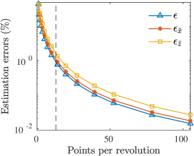
Figure 3: Estimation errors — $\epsilon_{\tilde{x}}$ and $\epsilon_{\tilde{z}}$ — as a function of the number of points per revolution. The Nyquist criterion returns at least 13 points per revolution to avoid undersampling effect.

IV.2 Observer of a dyad

Let us now move to the case of designing a state observer of a dyad of Rössler systems coupled through variable $y$ as sketched in Fig. 2(a) where nodes 1 and 2 are unidirectionally coupled as $1\rightarrowtail 2$. The observability analysis showed that the 6-dimensional state space $(x_{1},y_{1},z_{1},x_{2},y_{2},z_{2})$ associated with such a dyad is globally observable by only measuring variables $x_{2}$ and $y_{2}$ of node 2, that is, an observer can be constructed without singular observability manifold. Combining the governing equations for node 2 and a differentiator built from the reconstructed variable $\tilde{y}_{1}$ for node 1, we propose the following state observer $(\tilde{x}_{1},\tilde{y}_{1},\tilde{z}_{1},x_{2},y_{2},\tilde{z}_{2})$ for $\rho>0$:

$$\left|\begin{array}[]{l}\displaystyle\tilde{x}_{1}=-a_{1}\tilde{y}_{1}+\dot{\tilde{y}}_{1}\\[2.84544pt] \displaystyle\tilde{y}_{1}=y_{2}+\frac{1}{\rho}{[\dot{y}_{2}-x_{2}+(\rho-a_{2})y_{2}]}\\[2.84544pt] \displaystyle\tilde{z}_{1}=-\tilde{y}_{1}+a_{1}\dot{\tilde{y}}_{1}-\ddot{\tilde{y}}_{1}\\[2.84544pt] x_{2}\\[2.84544pt] y_{2}\\[2.84544pt] \displaystyle\tilde{z}_{2}=-\dot{x}_{2}-y_{2}\\[2.84544pt] \end{array}\right.$$ (30)

where $a_{1}$ and $a_{2}$ are the $a$ parameters of each node. Here, the observer returns the state at time $(k-1)\,{\rm d}t$.

An example of the performance of this observer as a function of the coupling strength $\rho$ is shown in Fig. 4 for a dyad with two identical Rössler systems ($a_{1}=a_{2}=0.432$) and with two different ones ($a_{1}=0.37$ and $a_{2}=0.432$). The ensemble average ($N=2$) of the errors in the estimation of the amplitude [Eq. (25)] and phase [Eq. (28)] of the two nodes are plotted together with the time averaged synchronization error computed as

$$S=\frac{1}{M}\frac{2}{N(N-1)}\sum_{n=1}^{M}\sum_{\begin{subarray}{c}i=1\\ i\neq j\end{subarray}}^{N}\|\mbox{x}_{i}(t_{n})-\mbox{x}_{j}(t_{n})\|$$ (31)

to help us correlating the synchronous state of the dyad and the easiness of the prediction: the estimation error of both the amplitude and phase keeps very low and stable above a given coupling value even when the nodes are not synchronous at all, and when the systems are not identical.

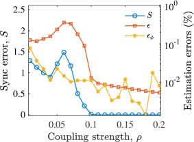
(a) Identical nodes

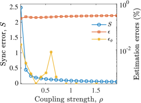
(b) Non-identical nodes

Figure 4: Dyad observer performance. Synchronization error $S$, amplitude error $\epsilon$, and phase reconstruction error $\epsilon_{\phi}$ as a function of the coupling $\rho$ of a dyad with (a) identical ($a_{1}=a_{2}=0.432$) and (b) non identical ($a_{1}=0.37$, $a_{2}=0.432$) Rössler oscillators. The sensor variables are $x_{2}$ and $y_{2}$. In each case, the synchronization error $S$ is read on the left vertical axis and the estimation errors in phase ($\epsilon_{\phi}$) and amplitude ($\epsilon$) are read (in percentages) on the right axis. Each point is the average of 10 different initial conditions. Other parameter values: $b=2$ and $c=4$.

V Network observer

In Sec. III.2, we concluded that it is not possible to retrieve the dynamics of more than two nodes from measurements in a single one and, for instance, when we consider the small motif of three nodes shown in Fig. 2(c), we have to perform measurements at least in two nodes for reconstructing the whole dynamics. The observer for this configuration needs to measure $x_{2}$ and $y_{2}$ to reconstruct the dyad and $y_{3}$ to reconstruct the third node. Note that the dyad is not isolated and one of the sensor variables $y_{2}$ is receiving input from $y_{3}$. Therefore, we propose to generalize the observer in Eq. (30) as follows:

$$\left|\begin{array}[]{l}\displaystyle\tilde{x}_{i}=-a_{i}\tilde{y}_{i}+\dot{\tilde{y}}_{i}\\[2.84544pt] \displaystyle\tilde{y}_{i}=y_{j}+\frac{1}{\rho}[\dot{y}_{j}-x_{j}-a_{j}y_{j}]+\sum_{l=1,l\neq i}^{N}A_{jl}(y_{j}-\tilde{y}_{l})]\\[2.84544pt] \displaystyle\tilde{z}_{i}=-\tilde{y}_{i}+a_{i}\dot{\tilde{y}}_{i}-\ddot{\tilde{y}}_{i}\\[2.84544pt] x_{j}\\[2.84544pt] y_{j}\\[2.84544pt] \displaystyle\tilde{z}_{j}=-\dot{x}_{j}-y_{j}\end{array}\right.$$ (32)

to reconstruct the dyads composed by nodes $i$ and $j$ embedded in a network (nodes $l$ are neighbors — according to the adjacency matrix — of the sensor $j$ except $i$), and the observer

$$\left|\begin{array}[]{l}\displaystyle\tilde{x}_{k}=-a_{k}y_{k}+\dot{y}_{k}\\[2.84544pt] \displaystyle y_{k}\\[2.84544pt] \tilde{z}_{k}=-y_{k}+a_{k}\dot{y}_{k}-\ddot{y}_{k}\end{array}\right.$$ (33)

for those nodes which have a sensor variable and are not paired. Due to the way these observers are constructed, the state (estimated or measured) of the nodes connected to the sensor variable of the dyad are needed prior the dyad reconstruction. Therefore, an iterative procedure is required for networks with $N>3$.

In the following, we will explore first the performance of Eqs. (32) and (33) for the case of a triad and later on we will extend our results to the case of larger networks.

V.1 Case of a triad

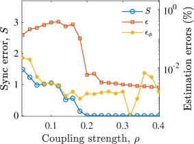
(a) Identical oscillators

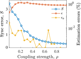
(b) Non-identical oscillators

Figure 5: Triad observer performance. Synchronization error $S$, amplitude reconstruction error $\epsilon$, and phase reconstruction error $\epsilon_{\phi}$ as a function of the coupling $\rho$ of a triad with (a) identical oscillators ($a_{1}=a_{2}=a_{3}=0.432$) and (b) non identical oscillators ($a_{1}=0.37$, $a_{2}=0.432$, and $a_{3}=0.52$). In each case, the synchronization error $S$ is read on the left vertical axis while the estimation errors ($\epsilon$ and $\epsilon_{\phi}$) are read (in percentages) on the right axis in log scale. Each point is the average from 10 different initial conditions.

We here consider the case of a triad of Rössler systems coupled through variable $y$ with the structure $1\rightarrowtail 2\leftarrowtail 3$ as shown in Fig. 2(c). In Fig. 5 we show the performance of the state observer with identical and non identical oscillators. The behavior is quite similar to that of a dyad but with slightly higher amplitude errors when the triad is composed of non identical systems.

Notice that the dynamics of node 2 is now far more complex than in the case of the dyad of non identical oscillators: the first-return map of the sensor $y_{2}$ in the triad [Fig. 6(b)] is very thick although the global shape still suggests two monotone branches as for the sensor $y_{2}$ in the dyad [Fig. 6(a)]. When the first-return map has a significant thickness $\epsilon$, there are more than one periodic orbit associated with a given orbital sequence: it is thus possible to have two different linking numbers — the number of times one periodic orbit cycles around the other — between orbits characterized by the same symbolic sequences, respectively. It is said that the attractor is $\epsilon$-topologically equivalent to the template which could be constructed if the thickness $\epsilon$ was removed (see Refs. Letellier, Dutertre, and Maheu, 1995; Mangiarotti, Sendiña-Nadal, and Letellier, 2018 for details). It appears rather challenging to retrieve the dynamics of node 1 (a period-2 limit cycle) from such a complex dynamics observed in node 2.

(a) Dyad with $1\rightarrowtail 2$

(b) Triad with $1\rightarrowtail 2\leftarrowtail 3$

Figure 6: Dynamics of the node 2 in the (a) dyad and (b) triad investigated in the right panels of Figs. 4 and 5, respectively, for $\rho=0.1$. State portraits (left panels) and the corresponding first-return maps (right panels) are depicted.

V.2 Observer hierarchical dependence

According to Corollary 2 and Proposition 3, an observer for a network can be constructed from Eqs. (32) and (33) by assembling the nodes by pairs and designate as sensor one member of each pair. There are multiple configurations for decomposing the network in pairs but in order to ensure a proper functioning of the algorithm and to unravel the coupling term in Eq. (32), we have to proceed in a hierarchical way, pairing first the nodes with lower degree; moreover, it reduces the possibilities and the pairing can be performed automatically.

We illustrate the pairing procedure for the network used in Ref. Sevilla-Escoboza and Buldú, 2016 and sketched in Fig. 7: its size is $N=28$ and its average degree is $\langle k\rangle=2.5$. There, paired nodes are encircled in blue, node sensors have the green contour and those nodes which must be fully reconstructed from another one have the red dashed contour. Note that some sensors are not paired (nodes 19 and 23). The algorithm producing this pairing is as follows:

1. Search for the nodes whose degree is equal to one and make a pair with their only neighbor. If two nodes with degree $k=1$ have the same neighbor (as nodes 22 and 23), then one of them is left unpaired (in the example is node 23).

2. Search for the nodes with $k=2$ and pair them with an unpaired neighbor with the lowest degree.

3. Repeat step 2 increasing the degree and stop up to the stage at which all nodes which can be paired are paired.

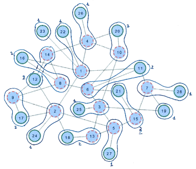
Figure 7: Graph of the random network with $N=28$ here investigated and extracted from Ref. Sevilla-Escoboza and Buldú (2016). Nodes are grouped by pairs (13) except nodes 19 and 23 which are left unpaired. Nodes encircled in green are sensors and those with red dashed contours are not. The rank $l$ of the layer for constructing the observer is also reported.

As a result of applying these steps, we end up with 13 pairs and 2 unpaired nodes, that is, $N_{m}=15$ sensor nodes ($\frac{N}{2}+1$). In particular, this means that we have to measure $m=N$ variables (the $x_{j}$ and $y_{j}$ variables in the paired sensors and the $y_{k}$ variable in the unpaired ones). To check whether this choice provides a global observability, we have to compute the symbolic observability coefficient of the reconstructed vector whose components are $\mbox{X}_{i}=\left[\begin{array}[]{ccc}y_{i}&\dot{y}_{i}&\ddot{y}_{i}\end{array}\right]^{\scriptscriptstyle\rm T}$ for the unpaired nodes $i=19,23$ and $\mbox{X}_{i}=\left[\begin{array}[]{cccccc}x_{i}&\dot{x}_{i}&y_{i}&\dot{y}_{i}&\ddot{y}_{i}&\stackrel{{\scriptstyle...}}{{y}}_{i}\end{array}\right]^{\scriptscriptstyle\rm T}$ for the paired sensors $i=11,12,16,17,18,20,21,22,24,25,26,27,$ and $28$. The symbolic observability coefficient is indeed equal to one and the analytical determinant of the observability matrix is Det ${\cal O}_{X}=\rho^{39}$, therefore validating our selection. The expression of this determinant would mean that the observability is strongly sensitive to the coupling value. Nevertheless, since nodes are grouped by pairs, the dependency on the coupling value should not be practically worst than the one observed for a pair of nodes, that is, depending on $\rho^{3}$.

Before actually applying the network observer described by Eqs. (32) for each pair $(i,j)$ and Eqs. (33) for each unpaired sensor node, let us show how the reconstruction works, especially regarding the coupling term in Eq. (32). For instance, to reconstruct node $i=8$ which is paired to the sensor $j=16$, we need to subtract from the variable $y_{16}$ the signal $y_{1}$ from its neighbor (see Fig. 7). But, to know this coupling signal, the dynamics of node $1$ needs to be reconstructed from node $22$, which is a sensor, before completing the reconstruction process. This hierarchical relationship is depicted in Fig. 8. From left to right, we uncover four different layers composed of nodes whose reconstruction depend on the precedent layers. In the first column of Fig. 8, the sensor nodes (paired and unpaired) are the nodes which do not need any other nodes to be fully reconstructed: they belong to the layer 1. The reconstruction of the dynamics of nodes belonging to layer 2 are obtained from the nodal dynamics in layer 1, and so on.

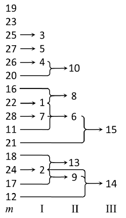
Figure 8: Hierarchical dependence of the observer. Nodal dynamics of the network shown in Fig. 7 is reconstructed layer by layer with the observer given by Eqs. (32) and (33). Layer 1 is composed exclusively by sensors. The reconstruction of the nodes belonging to layer 2 depends on those sensors and allow the reconstruction of those from layer 3, and so on.

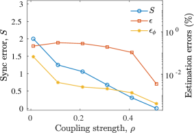
(a) Identical oscillators: $a_{i}=0.432$

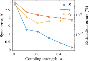
(b) Non-identical oscillators: $a_{i}=0.432\pm 5\%$

Figure 9: Small random network reconstruction. Synchronization error $S$, amplitude error $\epsilon$, and phase reconstruction error $\epsilon_{\phi}$ as a function of the coupling $\rho$ for the small random network with $N=28$ sketched in Fig. 7 for (a) identical and (b) non-identical oscillators. In each case, the synchronization error $S$ is read in the left vertical axis while the reconstruction errors (in percentage) are read in the right vertical axis. Each point is the average of 10 different initial conditions.

Once we solved the list of dependencies to reconstruct each node in our network shown in Fig. 7, we investigate the performance of the state observer by monitoring the error percentage in estimating the phase and amplitude of the nodal dynamics in the route to synchronization as the coupling parameter is increased. As expected, when nodes are identical ($a_{i}=0.432,\,\forall i$), all the errors are of the same order and keep low (less than $0.3\%$) as for dyads or triads of identical Rössler systems [Fig. 9(a)]; the phase and amplitude errors converge to zero when the oscillators synchronize to the same dynamics. Remarkably, when we inject a $5\%$ of parameter mismatch among the oscillators, the errors in the state estimation increase up to $15\%$ when the coupling is very low but they drop significantly down to the levels observed for identical systems when the network leaves the incoherent regime and synchronization is incipient ($\rho>0.1$).

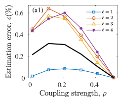
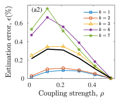
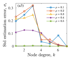
(a) Identical oscillators: $a_{i}=0.432$

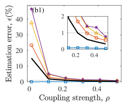
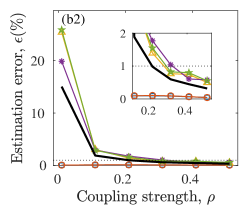
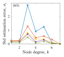
(b) Non-identical oscillators: $a_{i}=0.432\pm 5\%$

Figure 10: Dependence of the estimation error $\epsilon$ on the reconstruction layer $l$ [(a1) and (b1)] and on the node degree $k$ [(a2) and (b2)] as a function of the coupling strength for the small network investigated in Fig. 9. The standard deviation of the estimation error within each node degree $k$ is shown for several coupling values in (a3) and (b3). Legends on top panels apply to the bottom ones. Insets are blow ups of the main plot. Black curves show average quantities.

To explore in detail the role of the network topology in the network state reconstruction, we plot in Fig. 10 how the estimation error is distributed along the different layers and how it depends on the node degree $k$. Clearly, the best estimation is achieved in the first layer as this is the sensing layer and the reconstruction of these nodes involves only one (the $\tilde{z}_{j}$ of a paired sensor) or two (the $\tilde{x}_{k}$ and $\tilde{z}_{k}$ of an unpaired sensor) variables, while in the rest of layers, the three dimensional dynamics of the nodes has to be fully reconstructed. Nevertheless, the performance of the state observer does not deteriorates as we go deeper in the layer structure, with all layers exhibiting similar errors and of the same order as the error of the first one [Fig. 10(a1)]. This also holds for the network with non-identical oscillators [Fig. 10(b1)] although here, for very low coupling regimes ($\rho<0.1$), estimation errors are two orders of magnitude higher, with deeper layers having the largest errors. For $\rho>0.1$, errors drop and keep below $2\%$ and within the same order for all layers (see the inset in Fig.10(b1)). Figs. 10(a2) and 10(b2) show the same estimation errors as a function of the coupling strength but here each curve corresponds to the average error of all nodes having the same degree ranging between the minimum degree $k=1$, and the maximum $k=7$, being $k=3$ the average degree. Comparing 10(a2) and 10(b2), in both cases, the hierarchical procedure implemented in the reconstruction of the node dynamics is reflected here: nodes with degrees $k=1,2$ exhibit lower errors since those are most likely chosen as sensors, while those which are fully reconstructed belonging to deeper layers and having larger degrees, exhibit estimation errors larger than the average (black curve) but still low. However, not all the nodes having the same degree show similar estimation errors as evidenced in Figs. 10(a3) and 10(b3) where the dispersion of the estimation error is plotted as a function of the node degree for different coupling values. Independently of the coupling strength, those nodes whose connectivity is close to the average degree of the network $\langle k\rangle\sim 3$, show the largest standard deviation, meaning that they are unevenly reconstructed with some of them being well predicted while others do not.

V.3 Role of the degree distribution

To test the network observer in more complex connectivity architectures, we use standard network models as the Erdös-Rényi (ER) modelErdős and Rényi (1959) for random graphs and the Barabási-Albert modelBarabási and Albert (1999) to produce scale-free (SF) networks. We built network realizations as undirected graphs with $N=128$ nodes and average connectivities $\langle k\rangle=4$ and $\langle k\rangle=6$. Figure 11 summarizes the results for ER and SF networks showing that, in average, SF networks are easier to observe since the estimation errors in both phase and amplitude are lower: for intermediate coupling values, errors are around $1\%$ while for SF networks, they are about the half. Second, the network observer provides better estimations when topologies are more densely connected, as shown in both panels of Fig. 11 where curves for $\langle k\rangle=4$ are above the ones for $\langle k\rangle=6$. We also checked the effect of increasing the network size with no significant differences.

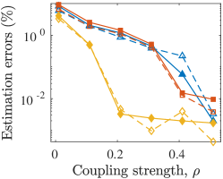
(a) Erdös-Rényi network

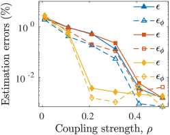
(b) Scale free network

Figure 11: Estimation error of the amplitude (continuous lines) and of the phase (dashed lines) for ER (a) and SF (b) networks of size $N=128$ (triangles) and $N=256$ (squares) with $\langle k\rangle=4$ as a function of the coupling strength. The effect of increasing the mean degree for $N=128$ is also plotted for $\langle k\rangle=6$ (diamonds). Each point is the average of 10 different network realizations and initial conditions.

The fact that the network state observer works better for SF than for ER networks lies, indeed, in the distinct degree distributions featured by these topologies. Figure 12 shows, for a particular coupling value and $\langle k\rangle=4$, how the estimation error in the reconstruction of the $N=128$ nodes, in each one of the 10 network realizations performed in Fig. 11, distributes as a function of the node connectivity $k_{i}$. Again, as in the example of the network with $N=28$ nodes shown in Figs. 10(a3) and 10(b3), the nodes whose connectivity is around the mean connectivity $\langle k\rangle=4$ are those exhibiting a larger variety of estimation errors. This is clear in Fig. 12(a) for both ER and SF networks. However, in the latter case, the small-degree nodes are the most numerous coexisting with a few highly connected hubs and, therefore, in comparison, the population of nodes with degree within the average is more reduced. An alternative way to inspect this is to plot how much error in the network state estimation is accumulated at nodes with degree smaller than a given $k$ [Fig. 12(b)]: it confirms the different contribution of the nodes depending on their connectivity.

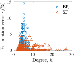
(a) Estimation error

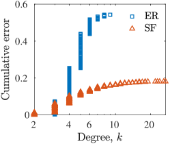
(b) Cumulative estimation error

Figure 12: Distribution of the estimation error of each node $\epsilon_{i}$ (a) and cumulative estimation error per node (b) as a function of the node degree for ER (squares) and SF (triangles) networks of size $N=128$ and $\langle k\rangle=4$. Notice in panel (b) the log scale of the horizontal axis. Data correspond to the averaged values plotted in Fig. 11 at $\rho=0.2$.

It is interesting to remark that while the number $N_{\rm sensors}$ of sensors is linearly correlated with the number $N$ of nodes, this is not the case for the number $N_{\rm layers}$ of layers which scales with $\sqrt{N}$ (Fig. 13). Regarding $N_{\rm sensors}$, the slope is close to 0.5, slightly increasing as the mean degree $\langle k\rangle$ increases (compare top panels for $\langle k\rangle=4$ and $\langle k\rangle=6$). As for the hierarchical reconstruction, the number $N_{\rm layers}$ of layers required is reduced as the average network connectivity is increased, saturating for large $N$. This would explain why the estimation errors are lower for networks with larger average degree (see Fig. 11).

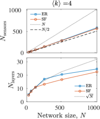
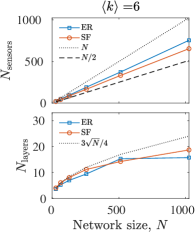
Figure 13: Number of sensors $N_{\rm sensors}$ and number of layers $N_{\rm layers}$ as a function of the network size ($N=\{28,64,128,256,512,1024\}$) for (left column) $\langle k\rangle=4$ and (right column) $\langle k\rangle=6$. In this figure, each point is an average of 20 networks.

VI Conclusion

We developed an algorithm to optimally place a set of sensors to render a network observable and designed an observer returning its real time state. Our procedure is based on an observability analysis adequate for nonlinear networks (here, the nodal dynamics is nonlinear). Although the coupling function between nodes is linear, it is found that the observer must be constructed in a layer by layer non-trivial way. The key point is to pair the nodes according to some basic topological rules which can be automatized for treating arbitrarily large networks. We found that a network can be observed with errors which are of the same order of magnitude as those yield by dyads or triads of nodes. The errors become large in networks with heterogeneous node dynamics as long as the synchronization level remains low. The performance of our network observer in the phase and amplitude reconstruction is very robust against different network architectures (degree distribution, link density and network size) and parameter mismatch in the node dynamics, opening, therefore, the perspective to devise a robust control law for networks, subject which is currently under investigation.