The multipolar structure of rotating boson stars

Abstract

The relativistic multipole moments provide a key ingredient to characterize the gravitational field around compact astrophysical objects. They play a crucial role in the description of the orbital evolution of coalescing binary systems and encode valuable information on the nature of the binary’s components, which leaves a measurable imprint in their gravitational-wave emission. We present a new study on the multipolar structure of a class of arbitrarily spinning boson stars with quartic self-interactions in the large coupling limit, where these solutions are expected to be stable. Our results strengthen and extend previous numerical analyses, showing that even for the most compact configurations the multipolar structure deviates significantly from that of a Kerr black hole. We provide accurate data for the multipole moments as functions of the object’s mass and spin, which can be directly used to construct inspiral waveform approximants and to perform parameter estimations and searches for boson star binaries.

I Introduction

The advent of gravitational-wave (GW) astronomy has opened new opportunities for tests of fundamental physics Barack et al. (2019). A cornerstone of this program is to use GW data to probe the nature of compact objects Cardoso and Pani (2019); Abbott et al. (2021); Maggio et al. (2021), and in particular to explore the possibility that astrophysical compact sources other than black holes (BH) and neutron stars can exist in the Universe. These hypothetical objects can provide a new portal to test a variety of particle and high-energy physics models Giudice et al. (2016); Pacilio et al. (2020) and could be an exotic explanation Bustillo et al. (2021) for the LIGO/Virgo “mass-gap events” (e.g. GW190814 Abbott et al. (2020a) and GW190521 Abbott et al. (2020b, a)) which do not fit naturally within the standard astrophysical formation scenarios for BHs and neutron stars.

Among the plethora of exotic compact objects Cardoso and Pani (2019), boson stars (BSs) stand out as one of the best motivated models arising from a concrete field theory. BSs are self-gravitating solitons, composed of either scalar Kaup (1968); Ruffini and Bonazzola (1969); Colpi et al. (1986) or vector Brito et al. (2016), massive complex fields, minimally coupled to Einstein’s gravity (see Jetzer (1992); Liebling and Palenzuela (2017) for some reviews). At variance with other models, for BSs the whole dynamics (including BS mergers Palenzuela et al. (2008, 2017); Bezares and Palenzuela (2018); Bustillo et al. (2021); Bezares et al. (2022) and nonlinear stability analysis Sanchis-Gual et al. (2019); Di Giovanni et al. (2020); Siemonsen and East (2021)) and phenomenology can be studied from first principles. They are therefore a natural target for GW searches.

Deviations in the GW inspiral signals with respect to the case of BH and neutron star binaries can be traced back to the so-called finite-size effects, which encode the properties of the object’s internal structure. In a post-Newtonian expansion of Einstein’s field equations for a binary system, the leading-order effect depending on the internal structure of the binary components is the spin-induced mass quadrupole moment, $M_{2}$ Poisson and Will (2014). According to General Relativity, if the object is a stationary BH, it must be axisymmetric and described by the Kerr solution. Due to the symmetries of the latter, the multipolar structure of a BH in General Relativity is encoded in a closed-form, elegant, relation Hansen (1974a)

$${M}_{\ell}^{\rm BH}+{i}{S}_{\ell}^{\rm BH}={M}^{\ell+1}\left({i}\chi\right)^{\ell}\,,$$ (1)

where ${M}_{\ell}$ (${S}_{\ell}$) are the Geroch-Hansen mass (current) multipole moments Geroch (1970); Hansen (1974a), ${M}\equiv M_{0}$ is the mass, $J\equiv{S}_{1}$ is the angular momentum, and $\chi\equiv{J}/{{M}^{2}}$ is the dimensionless spin. Introducing the dimensionless quantities ${\bar{M}}_{\ell}\equiv{M}_{\ell}/{M}^{\ell{+}1}$ and ${\bar{S}}_{\ell}\equiv{S}_{\ell}/{M}^{\ell{+}1}$, the only nonvanishing moments of the Kerr spacetime are

$${\bar{M}}_{2n}^{\rm BH}=(-1)^{n}\chi^{2n}\quad,\quad{\bar{S}}_{2n{+}1}^{\rm BH}=(-1)^{n}\chi^{2n{+}1}$$ (2)

for $n=0,1,2,...$. Besides the fact that the entire multipolar structure is completely determined only by the BH mass and spin, having ${M}_{\ell}=0$ (${S}_{\ell}=0$) when $\ell$ is odd (even) is a consequence of the equatorial symmetry of the Kerr metric, whereas the fact that all nonvanishing $\ell$-th multipoles (with $\ell\geq 2$) are proportional to $\chi^{\ell}$ is a peculiarity of the Kerr metric.

Any deviation from the above multipolar structure would imply that the underlying spacetime is not described by the Kerr solution. Therefore, measuring any multipole moment of a compact object in addition to the mass and spin would provide a null-hypothesis tests of the Kerr metric Psaltis (2008); Gair et al. (2013); Yunes and Siemens (2013); Berti et al. (2015); Cardoso and Gualtieri (2016); Barack et al. (2019); Cardoso and Pani (2019).

Going beyond null-hypothesis tests (e.g. if one wishes to perform model selection between the Kerr hypothesis and a more exotic model) requires computing the multipolar structure of alternative objects. In particular, the multipolar structure of BSs differs from that of a BH and depends on the underlying scalar self-interactions Ryan (1997); Pacilio et al. (2020), similarly to the case of neutron stars where the multipole moments depend on the underlying equation of state.

The multipolar structure of BSs with quartic scalar interactions was computed in a seminal paper by Ryan Ryan (1997) by using a perfect-fluid approximation scheme valid in the large self-coupling regime and implementing an iterative method to solve for Einstein’s equations in the stationary and axisymmetric case. The scope of this work is to extend Ryan’s analysis in order to accurately compute the leading-order moments (the mass quadrupole and the current octupole) in the entire parameter space of the model, and to provide accurate data, useful to build waveform templates Barack and Cutler (2007); Krishnendu et al. (2017); Krishnendu and Yelikar (2020) for actual searches and parameter estimation. Henceforth we adopt $G=c=1$ units.

II Theoretical setup

We consider stationary axisymmetric BSs as solutions of the Einstein–Klein-Gordon equations for a complex, massive, self-interacting scalar field minimally coupled to the gravitational sector Liebling and Palenzuela (2017). The Lagrangian governing the field dynamics reads

$${\cal L}_{\phi}=-\frac{1}{2}g^{\mu\nu}\phi^{*}_{,\mu}\phi_{,\nu}-\frac{1}{2}V(|\phi|^{2})\ ,$$ (3)

where $V(|\phi|^{2})$ is the scalar potential, which includes the mass term as well as self-interactions determining the object multipole moments. Varying the total action

$${\cal S}=\int d^{4}x\sqrt{-g}\left[\frac{R}{16\pi}-{\cal L}_{\phi}\right]\ ,$$ (4)

we obtain the field’s equations

$$G_{\mu\nu} =8\pi T_{\mu\nu}\,,$$ (5a)

$$\frac{1}{\sqrt{-g}}(\sqrt{-g}g^{\mu\nu}\phi_{,\mu})_{,\nu} =\frac{dV}{d|\phi|^{2}}\phi\,,$$ (5b)

where $g$ is the metric determinant and $T_{\mu\nu}$ is the canonical stress-energy tensor

$$T_{\mu\nu}=\frac{1}{2}(\phi^{*}_{,\mu}\phi_{,\nu}+\phi_{,\mu}\phi^{*}_{,\nu})-\frac{1}{2}g_{\mu\nu}\left[g^{\alpha\beta}\phi^{*}_{,\alpha}\phi_{,\beta}+V(|\phi|^{2})\right]\,.$$

We look for stationary and axisymmetric solutions of Eqns. (5). Using the set of coordinates $x^{\mu}=(t,r,\theta,\varphi)$ adapted to the isometry generators $\bigl{(}\frac{\partial}{\partial{t}},\frac{\partial}{\partial{\varphi}}\bigr{)}$, the metric and the stress-energy tensor of the solutions have no explicit dependence on $t$ and $\varphi$. Stationarity and axisymmetry require the scalar field to satisfy the ansatz

$$\phi=\phi_{0}(r,\theta)e^{i(s\phi-\Omega t)}\ ,$$ (6)

where the azimuthal winding number $s$ is an integer related to the BS total angular momentum and $\Omega>0$ is the field angular frequency Herdeiro and Radu (2018). We adopt quasi-isotropic coordinates for the metric of a stationary and axisymmetric spacetime

$$ds^{2}= -e^{\gamma+\rho}dt^{2}+e^{2\alpha}(dr^{2}+r^{2}d\theta^{2})$$

$$+e^{\gamma-\rho}r^{2}\sin{\theta}^{2}(d\varphi-\omega dt)^{2}\ ,$$ (7)

where the four metric functions $(\gamma,\rho,\alpha,\omega)$, depend on $(r,\theta)$ only. In this work we consider a specific family of massive BSs Colpi et al. (1986); Ryan (1997), featuring repulsive quartic self-interactions,

$$V(|\phi|^{2})=m^{2}|\phi|^{2}+\frac{1}{2}\lambda|\phi|^{4}\ .$$ (8)

Moreover we focus on the strong coupling limit $\lambda/m^{2}\gg 1$, in which the maximum mass supported by static configurations scales as Colpi et al. (1986)

$$M_{\textnormal{\rm max}}\sim 0.06\frac{\sqrt{\lambda\hbar}}{m_{s}^{2}}M_{p}^{3}\ ,$$ (9)

where $m_{s}=m\hbar$ is the mass of the boson and $M_{p}$ the Planck mass. Equation (9) shows that, for $\lambda\sim\mathcal{O}(\hbar^{-1})$ and $m_{s}$ in the range $1$–$100$ MeV, stellar configurations with $M_{\textnormal{\rm max}}$ in the range $10$–$10^{5}~{}M_{\odot}$ are supported. This is different from the case of mini BSs described by non-interacting scalars Kaup (1968); Ruffini and Bonazzola (1969), where the same mass range requires ultralight bosons. Moreover, large self-interactions are also expected to quench Siemonsen and East (2021) the instabilities observed in numerical simulations of rotating mini BSs Sanchis-Gual et al. (2019); Di Giovanni et al. (2020).

II.1 Perfect-fluid approximation in the strong-coupling limit

In the strong coupling regime the numerical integration of the stellar equations greatly simplifies. As discussed in Colpi et al. (1986), for spherically-symmetric solutions it is possible to identify two distinct regions in the object radial domain, corresponding to different behaviours of the field’s energy density. At large values of $r$ the BS features a tail region where $\phi$ decays exponentially as $\sim e^{-\sqrt{m^{2}-\Omega^{2}}r}/r$. At smaller $r$, an inner non-tail region sets up, where the field has significantly larger amplitude and most of the object’s mass is localized. In this zone $\phi$ varies on a very large scale, such that one can safely assume $\phi_{,r}\simeq 0$, while in the tail region, although $\phi_{,r}$ is in general not negligible, the field vanishes quickly due to the the exponential suppression and can be set to zero. We have numerically confirmed the validity of these assumptions, as shown in Fig. 1, which displays the radial profile of $\phi$ for two spherically symmetric BSs with the same frequency, built considering $\phi^{\textnormal{non-tail}}_{,r}\sim 0,\ \phi^{\textnormal{tail}}\sim 0$ (solid curve) and without any approximation (dashed curve).

In the spinning case, a further simplification can be made. Indeed, as noted in Ryan (1997), the symmetry of the solution suggests that the field stress-energy tensor should vary on the same scale when the star is rotating or not, such that in both cases derivatives with respect to the radial direction and the polar angle $\theta$ can be neglected in the non-tail region, while in general $\phi_{,\varphi}\neq 0$.

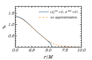
Figure 1: Scalar field profile for a spherically-symmetric massive BS with $\lambda/m^{2}=2500$, computed (i) neglecting radial derivatives of $\phi$ in the inner zone, and setting $\phi=0$ in tail zone (solid line) and (ii) with no approximations on the scalar field in the domain of integration (dashed line).

Setting $\phi_{,r}$ and $\phi_{,\theta}$ to zero in the stress-energy tensor and using the ansatz $\eqref{ansatz}$, we can recast $T_{\mu\nu}$ within the inner region in the following form

$$T_{\mu\nu}=(\epsilon+P)u_{\mu}u_{\nu}+Pg_{\mu\nu}\ ,$$ (10)

where

$$(u_{t},u_{r},u_{\theta},u_{\varphi})=A^{-1/2}(-\Omega,0,0,s)\,,$$ (11a)

$$A=\frac{g^{\alpha\beta}\phi^{*}_{,\alpha}\phi_{,\beta}}{|\phi|^{2}}\approx(-g^{tt}\Omega^{2}+2g^{t\varphi}\Omega s-g^{\varphi\varphi}s^{2})\,,$$ (11b)

and we identify the field’s pressure and energy density

$$P=\frac{1}{2}A|\phi|^{2}-\frac{1}{2}V(|\phi|^{2})\,,$$ (12a)

$$\epsilon=\frac{1}{2}A|\phi|^{2}+\frac{1}{2}V(|\phi|^{2})\,.$$ (12b)

In the tail region we assume that the scalar field is negligible, and we set $T_{\mu\nu}=0$. Therefore, within the entire domain of integration, the stress-energy tensor resembles that of a perfect fluid.

Note that, in the inner region of a rotating massive BS, the energy density develops a non-trivial topology. Indeed, neglecting the radial and polar derivatives of $\phi$, the scalar field satisfies the constraint equation

$$\Bigl{(}A\phi-\frac{dV}{d|\phi|^{2}}\phi\Bigr{)}=A\phi-m^{2}\phi-\lambda|\phi|^{2}\phi=0\,,$$ (13)

whose solutions are

$$\left\{\begin{aligned} |\phi|^{2}&=\frac{A-m^{2}}{\lambda}\quad&{\rm if}\quad A>m^{2}\,,\\ \phi&=0\quad&{\rm if}\quad A\leq m^{2}\,.\end{aligned}\right.$$

On the other hand, outside the inner region $|\phi|\sim 0$. Therefore, under the above approximations, the general expression for $|\phi|^{2}$ reads

$$|\phi|^{2} ={\rm max}[0,(-g^{tt}\Omega^{2}+2g^{t\varphi}\Omega s-g^{\varphi\varphi}s^{2}-m^{2})/\lambda]$$

$$={\rm max}\left[0,\frac{1}{\lambda}\left(\frac{(\Omega-s\omega)^{2}}{e^{\gamma+\rho}}-\frac{e^{\rho-\gamma}s^{2}}{r^{2}\sin{\theta}^{2}}-m^{2}\right)\right]\,.$$ (14)

The pressure, energy density, and four-velocity can be expressed in terms of $|\phi|^{2}$ as

$$P=\frac{1}{4}\lambda|\phi|^{4}\,,$$ (16a)

$$\epsilon=m^{2}|\phi|^{2}+\frac{3}{4}\lambda|\phi|^{4}\,,$$ (16b)

$$(u_{t},u_{r},u_{\theta},u_{\varphi})=\frac{(-\Omega,0,0,s)}{(\lambda|\phi|^{2}+m^{2})^{\frac{1}{2}}}\,.$$ (16c)

By combining Eqns. (14)-(16) one can see that the energy density of rotating BSs develops a toroidal shape, as evident from Eq. (14) which shows that $|\phi|^{2}$ is zero near the polar axis where $\sin\theta\approx 0$. This behaviour is displayed in Fig. 2 for a representative model. Note also that, in the absence of rotation, the torus degenerates into a spherical profile.

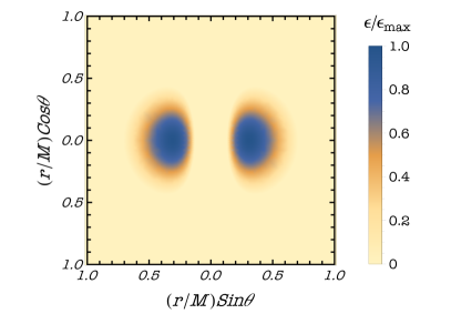
Figure 2: Vertical cross-section of a fast rotating BS with $M=0.04M_{B}$ and $\chi=J/M^{2}=1.3$. The scalar field energy density is normalized to its maximum value.

II.2 Coordinate rescaling

Our numerical analysis can be further simplified by a suitable change of variables which removes both $m$ and $\lambda$ from the field’s equations. In geometrical units $[\lambda]=[{\rm mass}]^{-2}$ and $[m]=[{\rm mass}]^{-1}$, such that the ratio $M_{B}\equiv\lambda^{\frac{1}{2}}/m^{2}$ has the dimension of a mass. We can then introduce the following dimensionless quantities:

$$\tilde{t}=t/M_{B}\quad\ , \quad\tilde{r}=r/M_{B}\,,$$ (17a)

$$\tilde{P}=PM_{B}^{2}\quad\ ,\quad\tilde{\epsilon}=\epsilon M_{B}^{2}\quad\ ,\quad\tilde{\omega}=\omega M_{B}\,.$$ (17b)

It is also convenient to define the dimensionless frequency $\tilde{\Omega}=\Omega/m\in(0,1)$, where for a BS $\Omega$ is always smaller than $m$, and the limit $\tilde{\Omega}\to 1$ corresponds to the non-relativistic (weak self-gravity) regime.

We can now scale the remaining dimensionless quantities by the ratio $\lambda^{1/2}/m$, in order to factor out the coupling constant from our equations:

$$\tilde{s}=\frac{m}{\lambda^{\frac{1}{2}}}s\quad\ ,\quad|\tilde{\phi}|^{2}=\frac{\lambda}{m^{2}}|\phi|^{2}\ .$$ (18)

Physical quantities can be restored after having solved the numerical problem by multiplying the dimensionless ones by different powers of $M_{B}$ to match the correct mass dimensions.

Hereafter we use $\tilde{s}$ as an input for the numerical integration of the field equations and threat it as a continuous parameter. This is a valid approximation for configurations with large values of $s$ since, by virtue of the first relation in Eq. (18), the magnitude of $\tilde{s}$ will be large compared to the spacing between two consecutive values, since $m/\lambda^{1/2}\ll 1$ Ryan (1997). Solutions with a given $\tilde{s}$ can also be regarded as configurations with small $s$. This, however, implies a constraint on the physical masses and spins of the dimensionful rescaled configurations, since the ratio $\lambda^{1/2}/m$ becomes necessarily a multiple of $1/\tilde{s}$. Moderate and fast spinning BSs with small $s$ cannot be obtained with our method, because they will have large $\tilde{s}$ and the first equation in (18) cannot be satisfied without violating the assumption $\lambda^{1/2}/m\gg 1$. Indeed BSs with small $s$ and large $\chi$ only exist outside the strong self-coupling limit. With the variable transformations in Eqns. (17)-(18), the problem translates in solving the Einstein equations for the metric specified by the line element

$$d\tilde{s}^{2}= -e^{\gamma+\rho}d\tilde{t}^{2}+e^{2\alpha}(d\tilde{r}^{2}+\tilde{r}^{2}d\theta^{2})$$

$$+e^{\gamma-\rho}\tilde{r}^{2}\sin{\theta}^{2}(d\varphi-\tilde{\omega}d\tilde{t})^{2}\ ,$$ (19)

where the dimensionless metric functions $\rho,\gamma$, and $\alpha$ are the same as in Eq. (7). The stress-energy tensor in dimensionless variables reads

$$\tilde{T}_{\mu\nu}=(\tilde{\epsilon}+\tilde{P})\tilde{u}_{\mu}\tilde{u}_{\nu}+\tilde{P}\tilde{g}_{\mu\nu}\,,$$ (20a)

$$(\tilde{u}_{\tilde{t}},\tilde{u}_{\tilde{r}},\tilde{u}_{\theta},\tilde{u}_{\varphi})=\frac{(-\tilde{\Omega},0,0,\tilde{s})}{(|\tilde{\phi}|^{2}+1)^{\frac{1}{2}}}\,,$$ (20b)

$$\tilde{\epsilon}=|\tilde{\phi}|^{2}+\frac{3}{4}|\tilde{\phi}|^{4}\quad\ ,\quad\tilde{P}=\frac{1}{4}|\tilde{\phi}|^{4}\,,$$ (20c)

and the scalar field constraint becomes

$$|\tilde{\phi}|^{2}={\rm max}\left[0,\frac{(\tilde{\Omega}-\tilde{s}\tilde{\omega})^{2}}{e^{\gamma+\rho}}-\frac{e^{\rho-\gamma}\tilde{s}^{2}}{\tilde{r}^{2}\sin{\theta}^{2}}-1\right]\ .$$ (21)

For the sake of clarity, unless specified differently in the text, hereafter we shall drop the tilde from rescaled variables, and we will assume that all quantities are dimensionless.

III A self-consistent method for equilibrium configurations

Finding BS solutions of the field equations (5) requires to solve an elliptic boundary value problem. To this aim we adopt the self-consisted method presented in Ryan (1997), as an application of Hachisu self-consistent field approach. The essence of this method lies in turning Einstein equations into an integral form which allows for an iterative resolution scheme. The first step toward the solution is writing the field equations in order to isolate on one side all operators having known Green functions and on the other side terms which can be regarded as effective sources.

The Einstein equations for $\rho,\gamma$ and $\omega$ can be written in the following form Komatsu et al. (1989):

$$\triangle(\rho e^{\frac{\gamma}{2}})=S_{\rho}(r,\mu)\,,$$ (22a)

$$\left(\triangle+\frac{1}{r}\frac{\partial}{\partial r}-\frac{1}{r^{2}}\mu\frac{\partial}{\partial\mu}\right)\gamma e^{\frac{\gamma}{2}}=S_{\gamma}(r,\mu)\,,$$ (22b)

$$\left(\triangle+\frac{2}{r}\frac{\partial}{\partial r}-\frac{2}{r^{2}}\mu\frac{\partial}{\partial\mu}\right)\omega e^{\frac{(\gamma-2\rho)}{2}}=S_{\omega}(r,\mu)\,,$$ (22c)

where $\mu=\cos{\theta}$, $\triangle$ is the Laplacian operator in spherical coordinates, and the sources appearing on the right hand side are known expressions of the metric functions and their derivatives.

The differential equation (22a) can be put in an integral form with the use of the three-dimensional Laplacian Green function:

$$\rho=-\frac{e^{-\frac{\gamma}{2}}}{4\pi}\int_{0}^{\infty}dr^{\prime}\int_{-1}^{1}d\mu^{\prime}\int_{0}^{2\pi}\frac{d\varphi^{\prime}r^{\prime 2}}{|r-r^{\prime}|}S_{\rho}(r^{\prime},\mu^{\prime})\ .$$ (23)

Using the expansion of $1/|r-r^{\prime}|$ in powers of $r^{\prime}/r$ (resp., $r/r^{\prime}$), valid for $r^{\prime}<r$ (resp., $r<r^{\prime}$), one obtains the following integro-differential equation:

$$\rho(r,\mu)=- e^{-\gamma/2}\sum_{n=0}^{\infty}\int_{0}^{\infty}dr^{\prime}R^{n}_{\rho}(r,r^{\prime})$$

$$\times\int_{0}^{1}d\mu^{\prime}P_{2n}(\mu)P_{2n}(\mu^{\prime})S_{\rho}(r^{\prime},\mu^{\prime})\,,$$ (24)

where $P_{2n}(\mu)$ are the Legendre polynomials and

$$R^{n}_{\rho}(r,r^{\prime})\equiv\frac{(r^{\prime})^{2n+2}}{r^{2n+1}}\Theta(r^{\prime}-r)+\frac{r^{2n}}{(r^{\prime})^{2n-1}}\Theta(r-r^{\prime})\,.$$ (25)

Analogous expressions can be found for Eqns. (22b)-(22c) with the same form as Eq. (24):

$$f_{i}\propto e^{\hat{v}(f)}\sum_{n=1}^{\infty}\int_{0}^{\infty}dr^{\prime} R^{n}_{f_{i}}(r,r^{\prime})$$

$$\times\int_{0}^{1}d\mu^{\prime}{M}^{n}_{f_{i}}(\mu,\mu^{\prime})S_{f_{i}}(r^{\prime},\mu^{\prime})\,,$$

where $f=(\rho,\gamma,\omega)$, $\hat{v}$ is a linear function of $f$, $R^{n}_{\gamma}(r,r^{\prime}),R^{n}_{\omega}(r,r^{\prime})$ have the structure of Eq. (25) and ${M}^{n}_{f}(\mu,\mu^{\prime})$ is an angular function including Legendre and associate Legendre polynomials. The asymptotic flatness conditions $\rho\sim\mathcal{O}(1/r)$, $\gamma\sim\mathcal{O}(1/r^{2})$, $\omega\sim\mathcal{O}(1/r^{3})$ for $r\to\infty$, are automatically satisfied if the source terms fall off sufficiently fast at large distances. We refer the reader to Appendix A for the full expression of the source terms.

Finally, the remaining metric function $\alpha$ can be determined by integrating the differential equation

$$\alpha_{,\mu}(r,\mu)=S_{\alpha}(r,\mu)\ ,$$ (26)

together with the condition that $\alpha=\frac{1}{2}(\gamma-\rho)$ at the pole, where $S_{\alpha}(r,\mu)$ is given by Eq. (43).

IV Multipole moments

Relativistic multipole moments characterize the structure of astrophysical compact objects, their gravitational field, including non-linear contributions Hansen (1974b) and their GW emission Poisson and Will (2014). The actual computation of the multipole moments greatly simplifies in a wide class of asymptotically Cartesian and mass centered coordinates Thorne (1980), which allows reading the multipole moments directly off the asymptotic behavior of the metric coefficients. Rotating axial (and equatorial) symmetry BSs are characterized by two families of scalar multipoles, the mass $\{M_{2i}\}_{i=0,\ldots\infty}$ and the current $\{S_{2i-1}\}_{i=1,\ldots\infty}$ moments, which can be extracted from the asymptotic behavior of the metric functions as in Ryan (1997):

$$\rho=-\sum_{n=0}^{\infty}\left[2\frac{M_{2n}}{r^{2n+1}}+\mathcal{O}\left(\frac{1}{r^{2n+2}}\right)\right]P_{2n}(\mu)\,,$$ (27a)

$$\omega=-\sum_{n=1}^{\infty}\left[\frac{2}{2n-1}\frac{S_{2n-1}}{r^{2n+1}}+\mathcal{O}\left(\frac{1}{r^{2n+2}}\right)\right]\frac{P_{2n-1}^{1}(\mu)}{\sin{\theta}}\,,$$ (27b)

with the lowest multipoles $M_{0},S_{1}\equiv J$, and $M_{2}$ corresponding to the mass, angular momentum, and quadrupole moment, respectively. Comparing Eqns. (27) with the explicit form of the metric in Eqns. (40a)-(40c) it is straightforward to identify the mass and current moments as integrals over the source terms $S_{\rho}$ and $S_{\omega}$:

$$M_{2n}=\frac{1}{2}\int_{0}^{r}dr^{\prime}(r^{\prime})^{2n+2}\int_{0}^{1}d\mu^{\prime}P_{2n}(\mu^{\prime})S_{\rho}(r^{\prime},\mu^{\prime})\,,$$ (28a)

$$S_{2n-1}=\frac{1}{4n}\int_{0}^{r}dr^{\prime}(r^{\prime})^{2n+2}$$

$$\quad\quad\times\int_{0}^{1}d\mu^{\prime}\sin{\theta^{\prime}}P_{2n-1}^{1}(\mu^{\prime})S_{\omega}(r^{\prime},\mu^{\prime})\,.$$ (28b)

However, as noticed in Pappas and Apostolatos (2012), the specific choice of radial coordinate leading to the line element (19) renders the identifications of the multipole moments with the coefficients $M_{2n}$ and $S_{2n}$ ambiguous. To correctly match the definition of multipole moments given by Geroch and Hansen Hansen (1974b), all terms in Eq. (27) with $n\geq 2$ must be corrected by adding a mass-spin dependent shift, yielding for the lowest moments:

$$M_{2}^{\textnormal{GH}}= M_{2}-\frac{4}{3}\Bigl{(}\frac{1}{4}+\frac{\gamma_{0}}{M_{0}^{2}}\Bigr{)}M_{0}^{3}\ ,$$ (29a)

$$S_{3}^{\textnormal{GH}}= S_{3}-\frac{12}{5}\Bigl{(}\frac{1}{4}+\frac{\gamma_{0}}{M_{0}^{2}}\Bigr{)}S_{1}M_{0}^{2}\ ,$$ (29b)

where $M^{\textnormal{GH}}_{2n}$ and $S^{\rm GH}_{2n-1}$ are Geroch-Hansen moments, and the coefficient $\gamma_{0}$ can be read-off from the asymptotic $1/r$ expansion

$$e^{\gamma}\sim\sqrt{\frac{\pi}{2}}\Bigl{[}\Bigl{(}1+\frac{\gamma_{0}}{r^{2}}\Bigr{)}T_{0}^{1/2}+\frac{\gamma_{2}}{r^{4}}T_{2}^{1/2}+....\Bigr{]}\ ,$$ (30)

where $T_{l}^{1/2}(\mu)$ are the Gegenbauer polynomials. We discuss the relevance of such corrections in Sec. VI, but we can anticipate that, for all the BS configurations that we have considered, the correction due to the shift in (29) is below $2\%$. For this reason, hereafter we will not distinguish between $\{M^{\rm GH}_{2n},S^{\rm GH}_{2n-1}\}$ and $\{M_{2n},S_{2n-1}\}$, discussing numerical results for the latter only.

It is convenient to introduce the reduced multipoles of order $n$:

$$\kappa_{2n}\equiv (-1)^{n}\frac{M_{2n}}{\chi^{2n}M_{0}^{2n+1}}=(-1)^{n}\frac{\bar{M}_{2n}}{\chi^{2n}}\ ,$$ (31)

$$\sigma_{2n-1}\equiv (-1)^{n+1}\frac{S_{2n-1}}{\chi^{2n-1}M_{0}^{2n}}=(-1)^{n+1}\frac{\bar{S}_{2n-1}}{\chi^{2n-1}}\ ,$$ (32)

with the leading multipoles being the reduced quadrupole and spin-octupole moments

$$\kappa_{2}=-\frac{M_{2}}{\chi^{2}M_{0}^{3}}\quad,\quad\sigma_{3}=-\frac{S_{3}}{\chi^{3}M_{0}^{4}}\ .$$ (33)

These quantities are regular in the small-$\chi$ limit, and depend on the mass $M\equiv M_{0}$ and the effective coupling $M_{B}=\lambda^{\frac{1}{2}}/m^{2}$ only through the dimensionless combination $M/M_{B}$. For a Kerr BH, $\kappa^{\textnormal{BH}}_{2n}=\sigma^{\textnormal{BH}}_{2n-1}=1$. As a comparison, for neutron stars $\kappa^{\textnormal{NS}}_{2}\sim 1\div 10$ depending on the internal composition Urbanec et al. (2013); Yagi and Yunes (2017). Furthermore, for a Kerr BH $\kappa^{\textnormal{BH}}_{2n}$ and $\sigma^{\textnormal{BH}}_{2n-1}$ are independent of the spin, while for neutron stars this is true only to ${\cal O}(\chi^{2})$.

V Numerical scheme

We have solved the system of equations for the metric functions and the scalar field discussed in Sec. III by using a self-consistent iterative scheme. The full solution depends on the radius and the polar angle, defined on a two-dimensional grid $(r,\theta)$ with a fixed size (see discussion in the next section). Numerical calculations have been coded in C according to the following iterative procedure:

1. We start by selecting an initial guess for the metric functions $(\rho,\gamma,\omega,\alpha)_{(1)}$, the angular frequency $\Omega$ and a specific value of $s$. The initial guess for the metric and the angular frequency corresponds to a solution of the field equations for a non-spinning, spherically symmetric BS as explained in Appendix B, while $s$ is initialized to a small but non-zero value, $s\sim 0.01$.

2. From such initial configuration, we compute the energy density, pressure and scalar field amplitude $(\epsilon,P,\phi)_{(1)}$ using Eqns. (20c)-(21).

3. We replace $(\rho,\gamma,\omega,\Omega,\epsilon,P,\phi)_{(1)}$ into the source terms on the right hand side of Eqns. (40), and perform the numerical integration, obtaining the values of the metric functions at the next step $(\rho,\gamma,\omega)_{(2)}$. The metric component $\alpha_{(2)}$ is obtained by direct integration of Eq. (26).

4. The energy density, pressure and scalar field amplitude $(P,\epsilon,\phi)_{(2)}$ are then computed from the above quantities, thus completing one full iteration of the procedure. The solution is then improved iteratively by repeating steps $1$-$4$ until the desired convergence is reached.

5. We use weighted averages of the metric functions to boost the convergence of the algorithm. Let $f_{(k)}$ collectively represent the values of each of the four components $(\rho,\gamma,\omega,\alpha)$ after the $k_{\textnormal{th}}$ iteration. Using $f_{(k)}$ to evaluate the source terms in Eq. (40) and integrating, we obtain the new values $\tilde{f}_{(k+1)}$, which one would naively use as the inputs for the next iteration. Instead, following Komatsu et al. (1989), we build the linear combinations

   $$f_{(k+1)}=a\tilde{f}_{(k+1)}+(1-a)f_{(k)}\ ,$$ (34)

   where $a\in(0,1)$ is a weight factor. The use of weighted averages avoids the solution to bounce among successive iterations. Hereafter we fix $a=1/3$, which we found to provide the best compromise between the speed and the accuracy of the convergence.

6. As a convergence criterion, we ask that the maximum relative difference between the values of all metric functions at two successive iterations, evaluated on the two-dimensional grid $(r,\theta)$, is smaller than a threshold $\delta$:

   $$\qquad\Delta f=\max\limits_{(r,\theta)}|f_{(i+1)}/f_{(i)}-1|<\delta\,,\quad f=(\rho,\gamma,\alpha,\omega)\ .$$ (35)

   For example, the algorithm needs about $150$ iterations for the solution to converge with a maximum relative error $\sim 10^{-5}$.

At each iteration, we adjust the input values of $\Omega$ and $s$ in such a way that the total mass and angular momentum, as determined by Eqns. (28), are kept fixed to their predetermined desired values. This adjustment is implemented through a two-dimensional Newton-Raphson method by solving the equations $M(\Omega_{k},s_{k})=M_{\textnormal{fin}}$ and $J(\Omega_{k},s_{k})=J_{\textnormal{fin}}$ for $(\Omega_{k},s_{k})$ at each $k$-th iteraction. This procedure allows us to choose, at the beginning of the numerical simulation, the mass and spin of the BS solution.

The metric functions are integrated on a two dimensional discrete grid for the coordinates $r$ and $\mu=\cos\theta$. We divide the angular domain into $n_{\mu}$ equally-spaced steps within $[0,1]$. We compactify the radial direction thorugh the change of coordinates

$$r\equiv r(q)=\frac{q}{1-q}\,,$$ (36)

such that the radial domain $r\in[0,\infty)$ is mapped into the finite domain $q\in[0,1)$. We perform the integration between $q(r_{0})=r_{0}/(r_{0}+1)$ and $q(r_{\textnormal{\rm max}})=r_{\textnormal{\rm max}}/(r_{\textnormal{\rm max}}+1)$, where $r_{0}=10^{-6}$ and $r_{\textnormal{\rm max}}=10$, which is typically two orders of magnitude larger than the radius of the BSs considered. We have verified that our results are stable for changes of both $r_{0}$ and $r_{\textnormal{\rm max}}$. The number of grid points in the radial direction was fixed to $n_{q}=600$, while in the angular domain we choose different setups depending on the spin. Small values of $\chi$ render the metric profile stiffer, and require a more refined lattice with larger values of $n_{\mu}$.

Derivatives in Eqns. (41) are numerically evaluated through a five-point central approximation, except near the inner (outer) boundary were we used forward (backward) derivatives. Integrals in Eqns. (40) are performed using the Simpson and the trapezoidal rule for the angular and the radial domain, respectively. We checked that higher order methods for both derivatives and integrals do not lead to significant changes in our results.

Integration near the pole for Eqn. (40a) and (40c) is simplified by resorting to the angular identities

$$\lim_{\theta\to 0}\frac{\sin{[(2n-1)\theta]}}{(2n-1)\sin{\theta}} =1\ ,$$ (37)

$$\lim_{\theta\to 0}\frac{P^{1}_{2n-1}(\cos{\theta})}{2n(2n-1)\sin{\theta}} =-\frac{(2n)!}{(n!)^{2}2^{2n}(2n-1)}\ .$$ (38)

Finally, we fix the values of the components in the sum of Eq. (40) to $n=10$.

VI Results

VI.1 Quadrupole and octupole moments of rotating massive BSs

We have studied the multipolar structure of arbitrarily rotating massive BS in the large coupling limit for different configurations specified by the spin parameter $\chi$ and by the object mass in units of $M_{B}$. To simplify the comparison with previous results in the literature, we include in our sample the range of masses considered in Ryan (1997) (we refer the reader to Appendix C for further comparisons).

We have carefully investigated how the obtained solutions are sensitive to the spacing of the numerical grid. We found that self-gravitating configurations are numerically stable under changes of the radial resolution (i.e. changes in $n_{q}$), while for small spins, typically $\chi\lesssim 0.1$, the integration becomes more sensitive to the angular resolution (i.e. to changes in $n_{\mu}$). At large spins $\chi\sim\mathcal{O}(1)$, the radius, frequency, and multipole moments are well determined and stable by choosing $n_{q}\sim n_{\mu}\sim\mathcal{O}(10^{2})$ and setting $n=10$ in Eq. (28a). Increasing the lattice density, as well as the cutoff value for $n$, typically yields changes of a few percent on the stellar structure. On the other hand, for slowly rotating BSs the calculation of multipole moments requires much larger values of $n_{\mu}\sim\mathcal{O}(10^{4})$, to converge to a stable solution. For this reason, to extract the quadrupole and octupole moments, we set the spacing of numerical grid to $n_{q}\times n_{\mu}=600\times 20000$ for $\chi\leq 0.1$ and $n_{q}\times n_{\mu}=600\times 1000$ for $\chi\geq 0.1$.

Moreover, as already discussed in Ryan (1997), we find that for $\chi=0$ the quadrupole moment does not vanish, leading to a (small) numerical offset $M^{\textnormal{(off)}}_{2}=M_{2}(\chi=0)$. This is a numerical artifact, as we know that $M_{2}\sim\chi^{2}+{\cal O}(\chi^{4})$. Therefore, we manually subtracted the offset from the raw values, i.e., we define the physical quadrupole moments as $M_{2}=M^{\textnormal{(raw)}}_{2}-M^{\textnormal{(off)}}_{2}$. The offset is negligible at large spin but it can spoil the $M_{2}\sim\chi^{2}$ scaling at small spins. The top panels of Fig. 3 show the reduced quadrupole moment $\kappa_{2}^{\textnormal{(raw)}}$ as obtained from the raw value of $M^{\textnormal{(raw)}}_{2}$, along with the corresponding value of the offset $\kappa^{\textnormal{(off)}}$, as a function of $n_{\mu}$ for a spinning BS with $\chi=0.1$ (left column) and $\chi=0.0075$ (right column). The mass of both configurations is fixed to $M/M_{B}=0.04$.

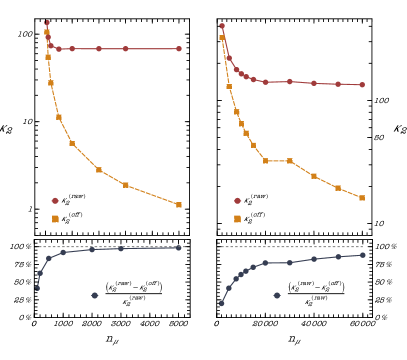
Figure 3: (Top panels) Data points identify raw values of the reduced quadrupole moment, as well as the numerical offset, as a function of the grid angular resolution. (Bottom panels) Reduced quadrupole moment normalized by its raw value as function of the angular resolution. Left and right panels refer to BSs with spin $\chi=0.1$ and $\chi=0.0075$, respectively, both with $M/M_{B}=0.04$.

While, for small $n_{\mu}$, $\kappa_{2}^{\textnormal{(raw)}}$ and $\kappa_{2}^{\textnormal{(off)}}$ have comparable magnitude, by increasing the value of $n_{\mu}$ the offset decreases monotonically and the effect of subtracting it becomes progressively less important. This is reflected in the bottom panels of Fig. 3, where we show that $\kappa_{2}/\kappa_{2}^{\textnormal{(raw)}}\to 1$ as the angular resolution increases. The convergence is faster for higher spins (left panel). For a low value of the spin (right panel), the offset $\kappa_{2}^{\textnormal{(off)}}$ contributes $\approx 25\%$ when $n_{\mu}=20000$, while the contribution reduces to $\approx 12\%$ when $n_{\mu}=60000$, the convergence being monotonic with $n_{\mu}$. This is coherent with the fact, anticipated before, that convergence of the solution requires $n_{\mu}\simeq 10^{3}$ and $n_{\mu}\simeq 2\times 10^{4}$ for $\chi\gtrsim 0.1$ and $\chi<0.1$, respectively. We stress that only after subtracting the offset does $M_{2}$ scale as $\chi^{2}$ at small spins.

We speculate that the convergence of $\kappa_{2}$ with $n_{\mu}$ can be traced back to the BS topology. Solutions with small spin resemble closely the nonrotating spherical configurations. But, however small be the spin, rotating BSs are toroidal and they have no continuum limit to the spherical topology of the nonrotating case (because, for a given mass and fixed coupling, $\chi$ can only assume discrete values). Configurations with spins close to the minimum value show a steep decrease of the energy density near the rotation axis, which requires a large number of angular points to be fully resolved.

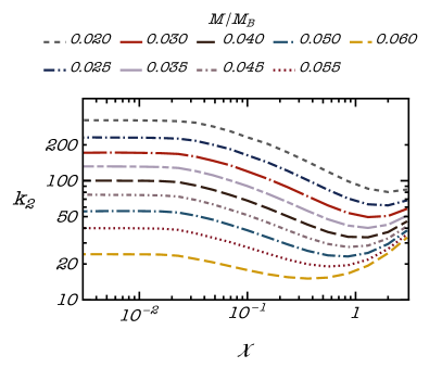
Figure 4: Reduced quadrupole moment $\kappa_{2}$ as a function of the dimensionless spin $\chi$ for different values of the BS mass in units of $M_{B}$. As a comparison, $\kappa_{2}^{\rm BH}=1$ for a Kerr BH with any spin.

The reduced quadrupole moments $\kappa_{2}$ for different BS configurations, as a function of the dimensionless mass parameter $M/M_{B}$ and of the spin $\chi$, are shown in Fig. 4. For small values of $\chi$, $\kappa_{2}$ is nearly independent of the spin, i.e. $M_{2}\propto\chi^{2}$, with the proportionality constant depending only on the object mass. In the stable branch, configurations with larger masses are also more compact. Correspondingly, for fixed spin, $\kappa_{2}$ decreases as the mass increases. Interestingly, $\kappa_{2}$ is nonmonotonic with $\chi$, but it shows a gradual decrease between $\chi\sim 0.03$ and $\chi\sim 1$, after which it grows rapidly Ryan (1997). Note that the spin can also exceed the Kerr bound, i.e. $\chi>1$.

The extraction of the reduced octupole moment $\sigma_{3}$ is more challenging due to the fact that, besides constant offsets, spurious numerical terms introduce additional nonphysical corrections at linear and quadratic order in the spin, spoiling the $\sigma_{3}\sim\chi^{3}+{\cal O}(\chi^{5})$ dependence. Also in this case the offset is negligible for highly-spinning configurations.

In order to isolate the physical contribution, we fit the behavior of the octupole moment with a cubic polynomial $S^{\textnormal{(raw)}}_{3}(\chi)=a_{0}+a_{1}\chi+a_{2}\chi^{2}+a_{3}\chi^{3}$ for different small values of the spin parameter. For all BS configurations considered, we find non-zero values for the three coefficients $a_{0,1,2}$, with $a_{0}\sim a_{2}\ll a_{1}$. After subtracting the constant, linear, and quadratic terms from the raw octupole moments, we recover the correct dependence $S_{3}\sim\chi^{3}$. Furthermore, to reduce the numerical noise, which can potentially affect the precision of the fit, we averaged over the last $50$ iterations of the algorithm, where $\Delta f$ in Eq. (35) oscillates about its minimum value. As for $M_{2}$, we find that the spurious coefficients $a_{0,1,2}$ decrease for higher angular resolution (i.e., for larger values of $n_{\mu}$).

However, the extraction of $\sigma_{3}$ is problematic for masses close to $M/M_{B}\simeq 0.06$, i.e., to the maximum mass of non rotating BSs. As already observed in Ryan (1997), the octupole moment is small for such masses and its accurate determination is prevented by numerical uncertainties. For this reason, we do not report the corresponding data. For the other configurations analyzed in Fig. 4, the reduced spin-octupole moment $\sigma_{3}=-S_{3}/\chi^{3}M^{4}$, obtained though the procedure described above, is shown in Fig. 5.

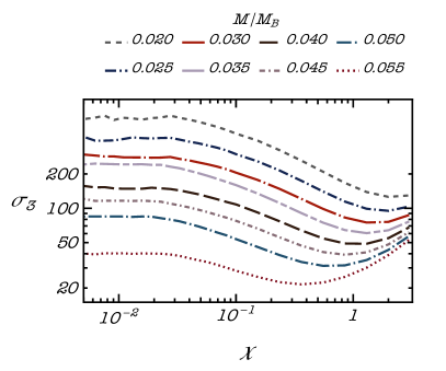
Figure 5: Reduced spin-octupole moment $\sigma_{3}$ as a function of the dimensionless spin $\chi$ for the same BS masses of Fig. 4. As a comparison, $\sigma_{3}^{\rm BH}=1$ for a Kerr BH with any spin.

As for the quadrupole moments, the curves are constant at small spins and exhibit a transition to a region with negative slope in correspondence roughly of the same values of $\chi$.

The data for the quadrupole and octupole as a function of the spin $\chi$ and mass $M/M_{B}$ are publicly available online web .

The values for $\kappa_{2}$ and $\sigma_{3}$ plotted above ignore the corrections in the definition of the Geroch-Hansen multipole moments, Eq. (29). We show that, indeed, these corrections introduce a shift at the (sub-)percent level and therefore they can be ignored at the current numerical precision. As a representative example, we focus on a specific BS configuration with mass $M=0.06M_{B}$ and different values of the spin. The corrections to the reduced quadrupole are shown in the last column of Table 1 for such models.

$\chi$	$\kappa_{2}$	$\kappa_{2}^{\rm new}$	${\rm correction}[\%]$
$0.1$	$22.4$	$22.1$	$\quad-1.4\%$
$0.2$	$15.7$	$15.6$	$\quad-0.5\%$
$0.5$	$15.2$	$15.3$	$\lesssim+0.1\%$
$0.8$	$16.4$	$16.4$	$\lesssim+0.1\%$
$1.0$	$17.4$	$17.5$	$\lesssim+0.1\%$
$1.3$	$19.3$	$19.4$	$\lesssim+0.1\%$
$2.0$	$24.6$	$24.6$	$\lesssim+0.05\%$

Table 1: Corrections to the reduced quadrupole moment derived in Pappas and Apostolatos (2012), for different value of the spin $\chi$ and $M=0.06M_{B}$.

We find that corrections to $\kappa_{2}$ are in general small, never exceeding a relative difference $\sim 2\%$, for the whole range of spins considered. The correction is larger for more compact configurations, therefore, given that $M=0.06M_{B}$ corresponds to the maximum value of the compactness for non-spinning BSs, changes in $\kappa_{2}$ are even smaller for lower values of the mass, as those analysed in Fig 4. This picture holds as well for $\sigma_{3}$, for which we find corrections smaller than $0.6\%$ for configurations near the maximum considered mass.

Finally, we have also checked that the first moments, namely the mass and spin as computed from Eqs. (27) agree with those obtained from the Komar integrals Poisson (2004):

$$M =-8\pi\int_{0}^{\infty}dr~{}\int_{0}^{1}d\cos{\theta}r^{2}e^{2\alpha+\gamma}\Bigl{(}T^{t}_{t}t^{t}-\frac{1}{2}Tt^{t}\Bigr{)}\,,$$

$$J =4\pi\int_{0}^{\infty}dr~{}\int_{0}^{1}d\cos{\theta}r^{2}e^{2\alpha+\gamma}T^{t}_{\varphi}\,.$$

VI.2 Maximum mass, compactness, ergoregions

Together with the multipolar structure, our framework allows describing various features of rotating BSs, such as the dependence of the maximum mass and of the compactness on the spin and frequency, as well as the presence of ergoregions.

Due to centrifugal forces which work against the gravitational collapse, rotating BSs can support larger masses, compared to their spherically symmetric counterparts, as also shown by the mass-frequency curves in Fig. 6 for four representative families of solutions with different value of $\tilde{s}$ .

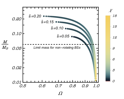
Figure 6: Boson star mass as a function of the frequency $\Omega$ for four different values of $\tilde{s}$. The color range of each configurations is mapped to the value of the $\chi$, with, darker (lighter) tones corresponding to smaller (larger) spins.

For a given value of $\tilde{s}$ the mass of each sequence of solutions grows as $\Omega$ decreases, until the maximum mass is reached, which is identified in our code by a failure of the algorithm to converge. Previous studies, which focused on massive BSs with non-rescaled winding number $s=1$, showed that such sequences are continuously connected for smaller frequencies to linearly unstable branches, in which $dM/d\Omega<0$ Herdeiro et al. (2015).

Figure 6 also shows the values of $\chi$ for the different configurations. Families of solutions with large $\tilde{s}$ have high spins as long as their frequency remains large. In particular, note that also configurations with $\chi\gg 1$ are allowed. As $\Omega$ decreases along the curve, the mass and compactness increase and $\chi$ rapidly falls, approaching a value $\chi(M_{\rm max})<1$. Moreover, $\chi(M_{\rm max})\simeq 1$ for all stars with $\tilde{s}$ large enough that significative rotation rate and compactnesses are approached along the curve.

Beside the maximum mass, we have also analysed the dependence on $\Omega$ of the BS compactness ${\cal C}=M/R$, with

$$R=R_{0}e^{\rho(R_{0},\pi/2)-\gamma(R_{0},\pi/2)}\ ,$$

being the perimetral radius and $R_{0}$ the stellar radius, i.e. the value of the $r-$coordinate for which the scalar field vanishes, marking the division between the tail and the non-tail region (see Sec. II.1). Figure 7 shows ${\cal C}$ as a function of the frequency, for the same stellar configurations considered before, plus other five with larger $\tilde{s}$.

Interestingly, for $\tilde{s}\lesssim 0.2$, the compactness depends linearly on the frequency and the relation is independent of the value of $\tilde{s}$ (or $\chi$). The latter only affects the minimum value of the frequency which can be reached by each family and the mass profile. This linear relation holds also for mini BSs in the stable branch, as can be appreciated examining the data in Delgado et al. (2020).

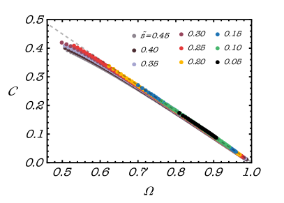
Figure 7: Colored dots identify the BS compactness as a function of the frequency for stars with $\tilde{s}$ in the range $(0.05,0.45)$. The mass for each family, varies between $M=0.06M_{B}$ and the maximum mass allowed by $\tilde{s}$. The dashed black line corresponds to a linear fit of the data for $\tilde{s}\leq 0.2$, i.e. ${\cal C}=0.9(1-\Omega)$.

All families with $\tilde{s}\gtrsim 0.25$ reach a maximum value ${\cal C}_{\rm max}\simeq 0.4$, smaller than the Buchdhal limit, around $\Omega_{\rm min}\simeq 0.5$.

Due to their large compactness, it is reasonable to expect that massive and fast spinning configurations develop ergoregions. Figure 8 shows indeed a sequence of BSs at the maximum mass allowed for a given value of $\chi$, which feature an ergoregion for sufficiently high spin. Notice that the first appearance of an ergoregion is for a configuration with $\chi\gtrsim 0.9$, ${\cal C}\gtrsim 0.30$. Such a BS has $\tilde{s}\sim 0.1$, which translates, in the $\lambda^{1/2}/m\gg 1$ limit, to a winding number $s\gg 1$. The ergoregion shown in Fig. 8 arise for solutions in the stable branch. However, although stable against radial perturbations, BSs with an ergoregion are unstable over longer timescales against nonspherical modes due to the so-called ergoregion instability Friedman (1978); Cardoso et al. (2008). An interesting followup of our work could be to quantify the instability time scale for our configurations.

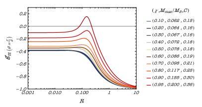
Figure 8: Metric component $g_{tt}$ as function of the radius on the equatiorial plane, for configurations corresponding to the maximum mass at a given spin $\chi$. For $(\chi,M)=(0.95,0.2M_{B})$ the $g_{tt}$ changes sign twice, revealing the presence of an ergoregion with toroidal topology.

VII Conclusions and discussion

In this work we constructed fully relativistic solutions of rotating BSs with quartic self-interactions within a perfect fluid approximation scheme, valid in the large self-coupling regime. The Einstein equations have been solved with a numerical C code implementing the iterative method described in Ryan (1997), which allows us to find configurations covering a wide portion of the parameter space, including those which are more relevant for phenomenology. Indeed, since the coupling constants are completely factored out from the numerical solution, each configuration corresponds to a family of BSs, sharing the same compactness and dimensionless spin but differing in the mass, the latter scaling linearly with the combination of the self-coupling and the boson’s mass defined in Sec. II.2.

We characterized the multipolar structure of these BSs up to the spin-octupole contribution, considering different sequences of compact configurations with constant mass, spanning a two-dimensional region in the mass-spin parameter space, including the slowly rotating regime. The values of the quadrupole and spin-octupole moments have been computed significantly more accurately than in previous work.

Our results, summarized in Fig. 4 and Fig. 5, confirm that the quadrupole moment is proportional to $\chi^{2}$ (as in the Kerr case) but only for slowly spinning BSs and that the constant reduced quadrupole moment in that regime has a minimum, causing the range of values of $\kappa_{2}$ to be not continuously connected to the BH value $\kappa_{2}^{\rm BH}=1$. We found such minimum, as well as the reduced multipoles, except for very large spin configurations, to be larger than what reported in previous work. We also confirmed that the spin-octupole is proportional to $\chi^{3}$ (as in the Kerr case) only for low spins.

Moreover, we discussed the masses and compactness of these objects, analyzing solutions with fixed rescaled winding number $\tilde{s}$ and for given values of the coupling constants. We showed that the maximum BS mass increases considerably for high $\tilde{s}$ and, as it grows, the maximum mass configuration is reached for lower and lower frequencies. The corresponding compactnesses approaches $\mathcal{C}\sim 0.4$, while the dimensionless spin parameter $\chi$ is close to unity. We found that some of these configurations have ergoregions in the branch connected to the Newtonian limit $\Omega\to 1$.

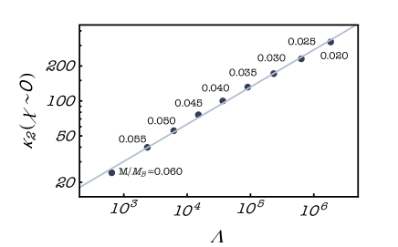
Figure 9: Reduced quadrupole moment $\kappa_{2}$ as a function of the tidal deformability for different values of the BS mass, in the low spin region, $\chi\lesssim 0.02$.

Among various theoretical and observational applications of our results, multipole moments have interesting phenomenological consequences related to the so-called universal relations Yagi and Yunes (2017). Indeed, it is known that approximated analytical relations exist between certain observables of a neutron star, such as the spin-induced quadrupole moment, the tidal deformability $\Lambda$, and the moment of inertia, which are roughly insensitive of the underlying equation of state Yagi and Yunes (2013). The same functional form of these relations holds also for the reduced quadrupole moment of slowly spinning massive BSs and its corresponding $\Lambda$, as we have recently shown Pacilio et al. (2020). The numerical calculations discussed in this paper allows to strengthen our previous result, obtained with limited data and accuracy. Using the fits for $\Lambda$ provided in Ref. Sennett et al. (2017), the $\kappa_{2}-\Lambda$ relation is shown Fig. 9, with the straight line identifying the semi-analytical fit

$$\log\kappa_{2}\simeq 1.2+0.32\log\Lambda\ .$$ (39)

We measured the distance of the data from the fit as the root mean square relative error $\sigma_{E}=0.01$, where $\sigma_{E}^{2}=\frac{1}{N}\sum_{n=1}^{N}(r_{E}^{i})^{2}$ and $r_{E}^{i}=\kappa_{2}^{i}-(1.2+0.32\Lambda^{i})$ are the residuals.

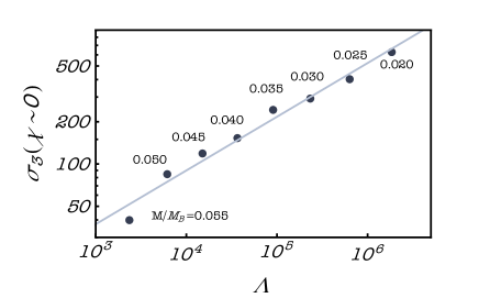
Figure 10: Reduced spin-octupole moment $\sigma_{3}$ as a function of the tidal deformability for different values of the BS mass, in the low spin region, $\chi\lesssim 0.02$. As for the quadrupole in Fig. 9, we show the best-fit line, corresponding to $\sigma_{3}\simeq 0.98+0.38\log\Lambda$. The distance from the fit is measured by $\sigma_{E}=0.03$.

We also used the data in Fig. 5 to explore the $\sigma_{3}-\Lambda$ relation. To reduce the numerical noise of $\sigma_{3}$ at low spins, we average $\sigma_{3}(\chi\sim 0)$ over $10$ points for $\chi\lesssim 0.02$, for each value of the mass. The data are shown in Fig. 10 and suggest that a simple linear relation exists as well between $\log\kappa_{2}$ and $\log\Lambda$. The relations discussed above might have many applications and are especially useful to break degeneracies among parameters that characterise gravitational waveforms Pacilio et al. (2020). On the theoretical side, proving that such $\kappa_{2}-\Lambda$ and $\sigma_{3}-\Lambda$ relations also exist for other scalar field interactions is an interesting and challenging task, which will shed light on the origin of the universality, and will be investigated in a followup publication. The results presented in this work are valid as long as the self-coupling is large, in which case the anisotropies of the star are negligible. Nonetheless the approach is not limited to BSs with $s\gg 1$, even if, for small $s$, only slowly rotating configurations can fully satisfy the requirement $\lambda/m^{2}\gg 1$ coherently with the first of Eqs. (18). The extension of these results to the generic coupling regime and to different BSs potentials will be explored elsewhere. Likewise, it would be interesting to extend our analysis to compute the multipolar structure of Proca stars Brito et al. (2016) or of Kerr BHs with bosonic hair Herdeiro and Radu (2014, 2015a, 2015b); Herdeiro et al. (2016).

Appendix A Field equations for arbitrarily spinning BSs in the large coupling limit

In this Appendix we provide the full integral form of the equations for the metric functions $\rho,\gamma$ and $\omega$, derived in Komatsu et al. (1989):

$$\rho(r,\mu)=-e^{-\gamma/2}\sum_{n=0}^{\infty}P_{2n}(\mu)\Bigg{[}\frac{1}{r^{2n+1}}\int_{0}^{r}dr^{\prime}(r^{\prime})^{2n+2}\int_{0}^{1}d\mu^{\prime}P_{2n}(\mu^{\prime})S_{\rho}(r^{\prime},\mu^{\prime})$$

$$+r^{2n}\int_{r}^{\infty}dr^{\prime}\frac{1}{(r^{\prime})^{2n-1}}\int_{0}^{1}d\mu^{\prime}P_{2n}(\mu^{\prime})S_{\rho}(r^{\prime},\mu^{\prime})\Bigg{]}\ ,$$ (40a)

$$\gamma(r,\mu)=-\frac{2}{\pi}e^{-\gamma/2}\sum_{n=1}^{\infty}\frac{\sin{[(2n-1)\theta]}}{(2n-1)\sin{\theta}}\Bigg{[}\frac{1}{r^{2n}}\int_{0}^{r}dr^{\prime}(r^{\prime})^{2n+1}\int_{0}^{1}d\mu^{\prime}\sin{[(2n-1)\theta^{\prime}]}S_{\gamma}(r^{\prime},\mu^{\prime})$$

$$+r^{2n-2}\int_{r}^{\infty}dr^{\prime}\frac{1}{(r^{\prime})^{2n-3}}\int_{0}^{1}d\mu^{\prime}\sin{[(2n-1)\theta^{\prime}]}S_{\gamma}(r^{\prime},\mu^{\prime})\Bigg{]}\ ,$$ (40b)

$$\omega(r,\mu)=-e^{\rho-\gamma/2}\sum_{n=1}^{\infty}\frac{P_{2n-1}^{1}(\mu)}{2n(2n-1)\sin{\theta}}\Bigg{[}\frac{1}{r^{2n+1}}\int_{0}^{r}dr^{\prime}(r^{\prime})^{2n+2}\int_{0}^{1}d\mu^{\prime}\sin{\theta^{\prime}}P_{2n-1}^{1}(\mu^{\prime})S_{\omega}(r^{\prime},\mu^{\prime})$$

$$+r^{2n-2}\int_{r}^{\infty}dr^{\prime}\frac{1}{(r^{\prime})^{2n-3}}\int_{0}^{1}d\mu^{\prime}\sin{\theta^{\prime}}P_{2n-1}^{1}(\mu^{\prime})S_{\omega}(r^{\prime}\mu^{\prime})\Bigg{]}\ .$$ (40c)

The functions $P_{n}(\mu)$ and $P_{n}^{m}(\mu)$ correspond to the Legendre and associate Legendre polynomials, respectively. The sources, defined in Eqns. (22a)-(22c), read

$$S_{\rho}(r,\mu)=e^{\gamma/2}\Bigg{\{}8\pi e^{2\alpha}(\epsilon+P)\frac{1+v^{2}}{1-v^{2}}+r^{2}(1-\mu^{2})e^{-2\rho}\Bigg{(}\omega^{2}_{,r}+\frac{1-\mu^{2}}{r^{2}}\omega^{2}_{,\mu}\Bigg{)}+\frac{1}{r}\gamma_{,r}-\frac{\mu}{r^{2}}\gamma_{,\mu}$$

$$+\frac{1}{2}\rho\Bigg{[}16\pi e^{2\alpha}P-\gamma_{,r}\Bigg{(}\frac{1}{2}\gamma_{,r}+\frac{1}{r}\Bigg{)}-\frac{1}{r^{2}}\gamma_{,\mu}\Bigg{(}\frac{1-\mu^{2}}{2}\gamma_{,\mu}-\mu\Bigg{)}\Bigg{]}\Bigg{\}}\ ,$$ (41a)

$$S_{\gamma}(r,\mu)=e^{\gamma/2}\Bigg{[}16\pi e^{2\alpha}P+\frac{\gamma}{2}\Bigg{(}16\pi e^{2\alpha}P-\frac{1}{2}\gamma^{2}_{,r}-\frac{1-\mu^{2}}{2r^{2}}\gamma^{2}_{,\mu}\Bigg{)}\Bigg{]}\ ,$$ (41b)

$$S_{\omega}(r,\mu)=e^{\gamma/2-\rho}\Bigg{\{}-16\pi e^{2\alpha+\rho}\frac{v(\epsilon+P)}{(1-v^{2})r\sin{\theta}}+\omega\Bigg{[}-8\pi e^{2\alpha}\frac{(1+v^{2})\epsilon+2v^{2}P}{1-v^{2}}-\frac{1}{r}(2\rho_{,r}+\frac{1}{2}\gamma_{,r})$$

$$+\frac{\mu}{r^{2}}(2\rho_{,\mu}+\frac{1}{2}\gamma_{,\mu})+\rho^{2}_{,r}-\frac{1}{4}\gamma^{2}_{,r}+\frac{1-\mu^{2}}{r^{2}}(\rho^{2}_{,\mu}-\frac{1}{4}\gamma^{2}_{,\mu})-r^{2}(1-\mu^{2})e^{-2\rho}\Bigg{(}\omega^{2}_{,r}+\frac{1-\mu^{2}}{r^{2}}\omega^{2}_{,\mu}\Bigg{)}\Bigg{]}\Bigg{\}}\ .$$ (41c)

The parameter $v$ entering in the previous expressions can be identified as the proper velocity with respect to the zero angular momentum observer and is given by:

$$v=\frac{s}{\Omega-s\omega}\frac{e^{\rho}}{r\sin{\theta}}\ .$$ (42)

Finally, the function $\alpha$ can be determined by solving

$$\alpha_{,\mu}=-\frac{1}{2}(\rho_{,\mu}+\gamma_{,\mu})+\{\frac{1}{2}[r^{2}(\gamma_{,rr}+\gamma^{2}_{,r})-(1-\mu^{2})(\gamma_{,\mu\mu}+\gamma^{2}_{,\mu})][-\mu+(1-\mu^{2})\gamma_{,\mu}]$$

$$+r\gamma_{,r}[\frac{1}{2}\mu+\mu r\gamma_{,r}+\frac{1}{2}(1-\mu^{2})\gamma_{,\mu}]+\frac{3}{2}\gamma_{,\mu}[-\mu^{2}+\mu(1-\mu^{2})\gamma_{,\mu}]$$

$$-r(1+r\gamma_{,r})(1-\mu^{2})(\gamma_{,r\mu}+\gamma_{,r}\gamma_{,\mu})-\frac{1}{4}\mu r^{2}(\rho_{,r}+\gamma_{,r})^{2}-\frac{1}{2}r(1+r\gamma_{,r})(1-\mu^{2})(\rho_{,r}+\gamma_{,r})(\rho_{,\mu}+\gamma_{,\mu})$$

$$+\frac{1}{4}\mu(1-\mu^{2})(\rho_{,\mu}+\gamma_{,\mu})^{2}+\frac{1}{4}r^{2}\mu(1-\mu^{2})\gamma_{,\mu}[r^{2}(\rho_{,r}+\gamma_{,r})^{2}-(1-\mu^{2})(\rho_{,\mu}+\gamma_{,\mu})^{2}]$$

$$+(1-\mu^{2})e^{-2\rho}(\frac{1}{4}r^{4}\mu\omega^{2}_{,r}+\frac{1}{2}r^{3}(1-\mu^{2})\omega_{,r}\omega_{,\mu}-\frac{1}{4}r^{2}\mu(1-\mu^{2})\omega^{2}_{,\mu}+\frac{1}{2}r^{4}(1-\mu^{2})\gamma_{,r}\omega_{,r}\omega_{,\mu}$$

$$-\frac{1}{4}r^{2}(1-\mu^{2})\gamma_{,\mu}[r^{2}\omega^{2}_{,r}-(1-\mu^{2})\omega^{2}_{,\mu}])\}/\{(1-\mu^{2})(1+r\gamma_{,r})^{2}+[\mu-(1-\mu^{2})\gamma_{,\mu}]^{2}\}\ .$$ (43)

with appropriate boundary conditions, which correspond to (26) with $S_{\alpha}(r,\mu)$ written explicitly on the right hand side.

Appendix B Initial data for rotating configurations

The self-consistent iterative scheme to build spinning BS solutions requires an initial guess for the metric functions $(\rho,\gamma,\omega,\alpha)$ and the frequency $\Omega$. For such initial data, we choose a solution describing a nonrotating BS with the same mass of the rotating configuration we want to obtain.
In the non-spinning limit, $\tilde{\omega}\to 0$, $e^{\gamma-\rho}=e^{2\alpha}$ and the metric reduces to

$$d\tilde{s}^{2}=-e^{2(\rho+\alpha)}d\tilde{t}^{2}+e^{2\alpha}(d\tilde{r}^{2}+\tilde{r}^{2}d\theta^{2}+\tilde{r}^{2}\sin{\theta}^{2}d\phi^{2})\ ,$$ (44)

in which the metric functions $\rho$ and $\alpha$ are independent of the angular variable $\mu=\cos\theta$. However, for spherically symmetric solutions, it proves useful to use a metric ansatz expressed in Schwarzschild-like coordinates:

$$ds^{2}=-e^{v(r)}dt^{2}+e^{u(r)}dr^{2}+r^{2}d\theta^{2}+r^{2}\sin{\theta}^{2}d\phi^{2}\ .$$ (45)

A relation between the metric functions $(\rho,\gamma,\alpha)$ and $(u,v)$ can be found once we determine a coordinate transformation that maps metric (45) into Eq. (44). Let’s start observing that assuming $\tilde{t}=t$ we have $\rho(\tilde{r})+\alpha(\tilde{r})=v(r)/2$. Moreover, from the spatial components of the metric:

$$\frac{d\tilde{r}}{r}=\frac{e^{\frac{u(r)}{2}}}{r}dr\ ,$$ (46)

which integrated, gives the desired map

$$\tilde{r}(r)\propto\cdot\textnormal{exp}\Bigl{[}\int_{r_{0}}^{r}\frac{e^{\frac{u(r^{\prime})}{2}}}{r^{\prime}}dr^{\prime}\Bigr{]}\ .$$ (47)

The proportionality constant has to be fixed by requiring that $\tilde{r}(r)\to r$ when $r\to\infty$. Summarizing, the mapping between the metric functions in the line elements (44) and (45) is given by

$$\alpha(\tilde{r}) =\log{\Bigl{(}\frac{r(\tilde{r})}{\tilde{r}}\Bigr{)}}\ ,$$

$$\gamma(\tilde{r}) =\rho(\tilde{r})+2\alpha(\tilde{r})\ ,$$

$$\rho(\tilde{r}) =\frac{1}{2}v(r(\tilde{r}))-\alpha(\tilde{r})\ .$$ (48)

Appendix C Comparison with previous results

We have tested the validity of our approach by comparing the numerical values obtained for the multipole moments of rotating BS, with previous results known in literature.

The left panel of Fig. 11 shows the reduced quadrupole moment $\kappa_{2}$ computed with our code, for five BS families with different masses, as a function of the spin $\chi$, compared against the values obtained in Ryan (1997). Each point represents a different BS solution derived by solving field’s equation on a grid $n_{q}\times n_{\mu}=1600\times 160$, which is the same adopted in Ryan (1997). Dashed lines correspond to data extracted from Fig. 4 of Ryan (1997). The values of the reduced quadrupole agree remarkably well on a wide range of spins, with an average relative discrepancy smaller than $7\%$ for all the considered BS masses.

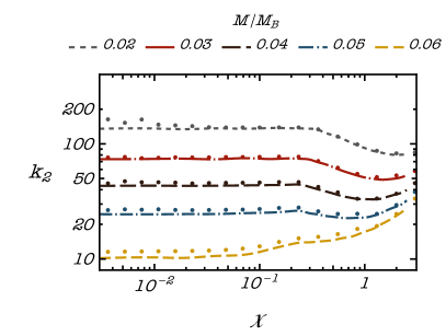
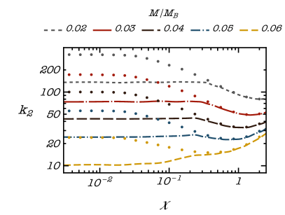
Figure 11: Left: Reduced quadrupole moment $\kappa_{2}$ as a function of the dimensionless spin $\chi$. Data points correspond to results obtained in this work setting the grid for the numerical integration of the field’s equation to $n_{q}\times n_{\mu}=1600\times 160$. Dashed curves refer to fit of data computed with the same set up in Ryan (1997). Right: same as the left panel but with higher angular resolution, $n_{q}\times n_{\mu}=1600\times 20000$. The low spin constant value is a factor of $\sim 2$ larger than in Ryan (1997) (dashed lines) , while there is a very good agreement for $\chi\gtrsim 0.3$.

However, as discussed in Sec. V-VI, calculations of the multipole moments are sensitive to the choice of the angular spacing $n_{\mu}$ for small values of the spin. By increasing $n_{\mu}$ we find indeed that the values of $\kappa_{2}$ (and $\sigma_{3}$) start deviating from those obtained in Ryan (1997).

In the right panel of Fig. 11 we show the reduced quadrupole computed using a $n_{q}\times n_{\mu}=1600\times 20000$ grid, again compared with data produced in Ryan (1997). While at high spins, the agreement between the two sets of results still hold, for rotating BSs with $\chi\lesssim 0.1$ our values are in general larger by a factor $\sim 2$ than those calculated by Ryan. We also note that for $M=0.06M_{B}$, the reduced quadrupole obtained with increased accuracy features an overall change in the behavior of $\kappa_{2}$ as a function of $\chi$. As explained in Sec. VI we have checked that our results saturate for large enough $n_{\mu}$. Indeed, doubling the grid resolution from $n_{\mu}=20000$ to $n_{\mu}=40000$ leads to variation in the multipole moments smaller than $5\%$ for $\chi\lesssim 0.1$ and even less for larger spins.

References

- Barack et al. (2019) L. Barack et al., Class. Quant. Grav. 36, 143001 (2019), arXiv:1806.05195 [gr-qc] .
- Cardoso and Pani (2019) V. Cardoso and P. Pani, Living Rev. Rel. 22, 4 (2019), arXiv:1904.05363 [gr-qc] .
- Abbott et al. (2021) R. Abbott et al. (LIGO Scientific, VIRGO, KAGRA), (2021), arXiv:2112.06861 [gr-qc] .
- Maggio et al. (2021) E. Maggio, P. Pani, and G. Raposo, (2021), arXiv:2105.06410 [gr-qc] .
- Giudice et al. (2016) G. F. Giudice, M. McCullough, and A. Urbano, JCAP 10, 001, arXiv:1605.01209 [hep-ph] .
- Pacilio et al. (2020) C. Pacilio, M. Vaglio, A. Maselli, and P. Pani, Physical Review D 102, 083002 (2020).
- Bustillo et al. (2021) J. C. Bustillo, N. Sanchis-Gual, A. Torres-Forné, J. A. Font, A. Vajpeyi, R. Smith, C. Herdeiro, E. Radu, and S. H. W. Leong, Phys. Rev. Lett. 126, 081101 (2021), arXiv:2009.05376 [gr-qc] .
- Abbott et al. (2020a) R. Abbott et al. (LIGO Scientific, Virgo), Astrophys. J. Lett. 900, L13 (2020a), arXiv:2009.01190 [astro-ph.HE] .
- Abbott et al. (2020b) R. Abbott et al. (LIGO Scientific, Virgo), Phys. Rev. Lett. 125, 101102 (2020b), arXiv:2009.01075 [gr-qc] .
- Kaup (1968) D. J. Kaup, Phys. Rev. 172, 1331 (1968).
- Ruffini and Bonazzola (1969) R. Ruffini and S. Bonazzola, Phys. Rev. 187, 1767 (1969).
- Colpi et al. (1986) M. Colpi, S. L. Shapiro, and I. Wasserman, Physical Review Letters 57, 2485 (1986).
- Brito et al. (2016) R. Brito, V. Cardoso, C. A. R. Herdeiro, and E. Radu, Phys. Lett. B 752, 291 (2016), arXiv:1508.05395 [gr-qc] .
- Jetzer (1992) P. Jetzer, Phys. Rept. 220, 163 (1992).
- Liebling and Palenzuela (2017) S. L. Liebling and C. Palenzuela, Living Reviews in Relativity 20, 5 (2017).
- Palenzuela et al. (2008) C. Palenzuela, L. Lehner, and S. L. Liebling, Phys. Rev. D 77, 044036 (2008), arXiv:0706.2435 [gr-qc] .
- Palenzuela et al. (2017) C. Palenzuela, P. Pani, M. Bezares, V. Cardoso, L. Lehner, and S. Liebling, Phys. Rev. D 96, 104058 (2017), arXiv:1710.09432 [gr-qc] .
- Bezares and Palenzuela (2018) M. Bezares and C. Palenzuela, Class. Quant. Grav. 35, 234002 (2018), arXiv:1808.10732 [gr-qc] .
- Bezares et al. (2022) M. Bezares, M. Bošković, S. Liebling, C. Palenzuela, P. Pani, and E. Barausse, (2022), arXiv:2201.06113 [gr-qc] .
- Sanchis-Gual et al. (2019) N. Sanchis-Gual, F. Di Giovanni, M. Zilhão, C. Herdeiro, P. Cerdá-Durán, J. A. Font, and E. Radu, Phys. Rev. Lett. 123, 221101 (2019), arXiv:1907.12565 [gr-qc] .
- Di Giovanni et al. (2020) F. Di Giovanni, N. Sanchis-Gual, P. Cerdá-Durán, M. Zilhão, C. Herdeiro, J. A. Font, and E. Radu, Phys. Rev. D 102, 124009 (2020), arXiv:2010.05845 [gr-qc] .
- Siemonsen and East (2021) N. Siemonsen and W. E. East, Physical Review D 103, 044022 (2021).
- Poisson and Will (2014) E. Poisson and C. Will, Gravity: Newtonian, Post-Newtonian, Relativistic (Cambridge University Press, 2014).
- Hansen (1974a) R. O. Hansen, J. Math. Phys. 15, 46 (1974a).
- Geroch (1970) R. P. Geroch, J. Math. Phys. 11, 2580 (1970).
- Bianchi et al. (2020) M. Bianchi, D. Consoli, A. Grillo, J. F. Morales, P. Pani, and G. Raposo, Phys. Rev. Lett. 125, 221601 (2020), arXiv:2007.01743 [hep-th] .
- Bianchi et al. (2021) M. Bianchi, D. Consoli, A. Grillo, J. F. Morales, P. Pani, and G. Raposo, JHEP 01, 003, arXiv:2008.01445 [hep-th] .
- Fransen and Mayerson (2022) K. Fransen and D. R. Mayerson, (2022), arXiv:2201.03569 [gr-qc] .
- Loutrel et al. (2022) N. Loutrel, R. Brito, A. Maselli, and P. Pani, (2022), arXiv:2203.01725 [gr-qc] .
- Psaltis (2008) D. Psaltis, Living Rev. Rel. 11, 9 (2008), arXiv:0806.1531 [astro-ph] .
- Gair et al. (2013) J. R. Gair, M. Vallisneri, S. L. Larson, and J. G. Baker, Living Rev. Rel. 16, 7 (2013), arXiv:1212.5575 [gr-qc] .
- Yunes and Siemens (2013) N. Yunes and X. Siemens, Living Rev. Rel. 16, 9 (2013), arXiv:1304.3473 [gr-qc] .
- Berti et al. (2015) E. Berti et al., Class. Quant. Grav. 32, 243001 (2015), arXiv:1501.07274 [gr-qc] .
- Cardoso and Gualtieri (2016) V. Cardoso and L. Gualtieri, Class. Quant. Grav. 33, 174001 (2016), arXiv:1607.03133 [gr-qc] .
- Ryan (1997) F. D. Ryan, Physical Review D 55, 6081 (1997).
- Barack and Cutler (2007) L. Barack and C. Cutler, Phys. Rev. D 75, 042003 (2007), arXiv:gr-qc/0612029 .
- Krishnendu et al. (2017) N. V. Krishnendu, K. G. Arun, and C. K. Mishra, Phys. Rev. Lett. 119, 091101 (2017), arXiv:1701.06318 [gr-qc] .
- Krishnendu and Yelikar (2020) N. V. Krishnendu and A. B. Yelikar, Class. Quant. Grav. 37, 205019 (2020), arXiv:1904.12712 [gr-qc] .
- Herdeiro and Radu (2018) C. A. R. Herdeiro and E. Radu, International Journal of Modern Physics D 27, 1843009 (2018).
- Komatsu et al. (1989) H. Komatsu, Y. Eriguchi, and I. Hachisu, Monthly Notices of the Royal Astronomical Society 237, 355 (1989).
- Hansen (1974b) R. O. Hansen, Journal of Mathematical Physics 15, 46 (1974b).
- Thorne (1980) K. S. Thorne, Reviews of Modern Physics 52, 299 (1980).
- Pappas and Apostolatos (2012) G. Pappas and T. A. Apostolatos, Physical Review Letters 108, 231104 (2012).
- Urbanec et al. (2013) M. Urbanec, J. C. Miller, and Z. Stuchlik, Mon. Not. Roy. Astron. Soc. 433, 1903 (2013), arXiv:1301.5925 [astro-ph.SR] .
- Yagi and Yunes (2017) K. Yagi and N. Yunes, Phys. Rept. 681, 1 (2017), arXiv:1608.02582 [gr-qc] .
- (46) https://web.uniroma1.it/gmunu/.
- Poisson (2004) E. Poisson, A Relativist’s Toolkit: The Mathematics of Black-Hole Mechanics (Cambridge University Press, Cambridge, 2004).
- Herdeiro et al. (2015) C. A. Herdeiro, E. Radu, and H. Rúnarsson, Physical Review D 92, 084059 (2015).
- Delgado et al. (2020) J. F. Delgado, C. A. Herdeiro, and E. Radu, Journal of Cosmology and Astroparticle Physics 2020 (06), 037.
- Buchdahl (1959) H. A. Buchdahl, Phys. Rev. 116, 1027 (1959).
- Friedman (1978) J. L. Friedman, Communications in Mathematical Physics 63, 243 (1978).
- Cardoso et al. (2008) V. Cardoso, P. Pani, M. Cadoni, and M. Cavaglia, Phys.Rev. D77, 124044 (2008), arXiv:0709.0532 [gr-qc] .
- Yagi and Yunes (2013) K. Yagi and N. Yunes, Physical Review D 88, 023009 (2013), arXiv: 1303.1528.
- Sennett et al. (2017) N. Sennett, T. Hinderer, J. Steinhoff, A. Buonanno, and S. Ossokine, Phys. Rev. D 96, 024002 (2017), arXiv:1704.08651 [gr-qc] .
- Herdeiro and Radu (2014) C. A. R. Herdeiro and E. Radu, Phys. Rev. Lett. 112, 221101 (2014).
- Herdeiro and Radu (2015a) C. A. R. Herdeiro and E. Radu, Int. J. Mod. Phys. D 24, 1542014 (2015a), arXiv:1504.08209 [gr-qc] .
- Herdeiro and Radu (2015b) C. Herdeiro and E. Radu, Class. Quant. Grav. 32, 144001 (2015b), arXiv:1501.04319 [gr-qc] .
- Herdeiro et al. (2016) C. Herdeiro, E. Radu, and H. Rúnarsson, Class. Quant. Grav. 33, 154001 (2016), arXiv:1603.02687 [gr-qc] .