New LZ and PW(Z) relations of RR Lyrae stars calibrated with Gaia EDR3 parallaxes

Abstract

We present new luminosity-metallicity ($LZ$; $M_{V}-\rm[Fe/H]$ and $M_{G}-\rm[Fe/H]$) relations and, for the first time, empirical, Gaia three-band ($G,G_{\rm BP},G_{\rm RP}$) period-Wesenheit-metallicity ($PWZ$) relations of RR Lyrae stars (RRLs) derived using a hierarchical Bayesian approach and new accurate parallaxes published for these variables in the Gaia Early Data Release 3 (EDR3). In a previous study we obtained Bayesian hierarchically-derived $LZ$ relations from a sample of about four hundred Milky Way field RRLs with $G$-band light curves and trigonometric parallaxes published in the Gaia Data Release 2 (DR2), using $V$ mean magnitudes, metallicities, absorptions and pulsation periods available in the literature. We now extend that study in two directions. Firstly, we update our previous results using trigonometric parallaxes from Gaia EDR3 and incorporate the Bayesian analysis of a first empirical $PWZ$ relation derived using those field RRLs with $G$, $G_{\rm BP}$ and $G_{\rm RP}$ time-series photometry available in Gaia DR2. Secondly, we use Bayesian inference to derive $LZ$ relations and empirical PW Gaia three-band relations from 385 RRLs belonging to 15 Milky Way globular clusters (GC) with literature-compiled spectroscopic metallicities ranging from $-$0.36 to $-2.39$ dex and prior distances extending from $2.2$ to $41.2$ kpc. From the samples of RRLs analysed in this paper we infer a mean Gaia EDR3 zero-point offset of $-$0.028 mas with median values ranging from $-$0.033 ($LZ$ and $PWZ$ models for field stars) to $-$0.024 mas ($LZ$ model in the $V$-band for GC RRLs).

1 Introduction

On December 2020, the early installment of the Gaia third data release (Early Data Release 3, EDR3; Gaia Collaboration et al. 2020) published updated astrometry and photometry for nearly 2 billion sources down to a limiting magnitude $G\sim$ 21 mag. Among them, are tens of thousands of RR Lyrae stars (RRLs). The number and accuracy of RRL distances directly estimated from parallax measurements have been steadily increasing with subsequent Gaia Data Releases, leading to a renewed role of RRLs as standard candles of the cosmic distance ladder. At the same time, the intriguing discord between the value of the Hubble constant, $H_{0}$, from measurements of the cosmic microwave background anisotropy and from distance indicators in the local Universe (Verde et al. 2019, and references therein, but see the paper by , for a different view); Di Valentino 2021, and references therein, but see the paper by , for a different view); Riess et al. 2021a, and references therein, but see the paper by , for a different view); Riess et al. 2021b, and references therein, but see the paper by , for a different view) has shown the need for both reducing uncertainties and systematics in the stellar standard candles traditionally used in the distance ladder measurement of $H_{0}$ (the Population I Cepheids) and for exploring alternative paths to $H_{0}$ independent of Cepheids, such as that represented by Population II RRLs (Beaton et al., 2016, and references therein) with luminosity calibrated on Gaia parallaxes.
A number of different characteristic relations from the optical to the mid-infrared bands make RRLs standard candles widely used to measure distances within the Milky Way (MW) and its nearest neighbours up to about 1 Mpc in distance (see e.g. Ordoñez & Sarajedini, 2016). In optical passbands the absolute visual magnitude of RRLs is linked to the metallicity by a relation, traditionally known as Luminosity - Metallicity ($LZ$) relation, $M_{V}-{\rm[Fe/H]}$ (see e.g. Sandage, 1993; Caputo et al., 2000; Cacciari & Clementini, 2003; Clementini et al., 2003; Catelan et al., 2004; Marconi et al., 2015; Muraveva et al., 2018, and references therein) while, from red ($R$ and $I$ bands) to near-mid infrared passbands, RRLs follow Period-Luminosity ($PL$), Period-Luminosity-Metallicity relations ($PLZ$, see e.g. Longmore et al., 1986; Bono et al., 2003; Catelan et al., 2004; Sollima et al., 2006; Coppola et al., 2011; Madore et al., 2013; Braga et al., 2015; Marconi et al., 2015; Muraveva et al., 2015; Neeley et al., 2019, and references therein). Intrinsic errors and systematics affecting distances based on the $LZ$ relation are widely discussed in the literature (see e.g. Bono, 2003, and references therein). They include uncertainty of the metallicity measurements, lack of information about the $\alpha$-element enhancement, dispersion of the RRL mean luminosity caused by poor knowledge reagarding the off zero-age horizontal branch (ZAHB) evolution of these variables and, also, a possible non-linearity of the relation itself over the whole metallicity range spanned by the MW field RRLs. Although the $PL(Z)$ relations for red and infrared passbands have well known advantages in comparison with the optical $LZ$ relation (primarily a smaller dependence of the luminosity on metallicity and evolutionary effects and a much weaker impact of reddening at infrared passbands), uncertainties on these quantities still affect the accuracy with which the $PLZ$ coefficients are determined and the dispersion of the relations themselves (see e.g. Marconi et al., 2015; Neeley et al., 2017, for a discussion). The introduction of the Wesenheit function by van den Bergh (1975) and Madore (1982) has allowed to minimize the reddening dependence of the $PL$ relation, by defining a Period-Wesenheit ($PW$) relation which is reddening-free by construction, assuming that the extinction law is known. However, all RRL relations need a better determination of their coefficients to reduce systematics and an accurate calibration of their zero points to firmly anchor the distance ladder.

The advent of Gaia has triggered new empirical and theoretical investigations of the RRL $PL(Z)$, $PW(Z)$ and $LZ$ relations and improved geometrical calibrations using Gaia astrometry and photometry. In the recent years there has also been an increasing application of Bayesian methods to improve the cosmic distance ladder. In particular, Bayesian hierarchical methods have been used to increase the potential of type Ia supernovae (SN Ia, Mandel et al., 2009) and red clump (RC) stars (Hawkins et al., 2017; Hall et al., 2019) as distance indicators, to obtain a first calibration of the $PL$, $PLZ$ and $PW$ relations of Cepheids and the $LZ$ relation of RRLs based on parallaxes from the Tycho-Gaia Astrometric Solution (TGAS; Gaia Collaboration et al. 2017), to constrain the $PLZ$ relations of RRLs (Sesar et al., 2017; Muraveva et al., 2018; Delgado et al., 2019) and to clarify the Hubble constant tension (Feeney et al., 2018). The main advantage of the Bayesian hierarchical method, a model-based machine learning approach (Bishop, 2013; Ghahramani, 2015), is the use of a network model that includes problem parameters and measurements, dependency relationships between them and prior information gathered from previous studies. In this way, when the inference is carried out, it is guaranteed that the observational uncertainties are simultaneously propagated through the network and the uncertainties on the parameters of interest are estimated in a way that is consistent with the measurement uncertainties.
Applying a Bayesian modelling approach along with Gaia DR2 parallaxes and $G$-band time-series photometry and, $V$-band time-series photometry from literature, in Muraveva et al. (2018) we derived new $M_{V}-{\rm[Fe/H]}$ and infrared $PLZ$ relations using a sample of about 400 RRLs in the field of the MW. In that work, we also presented for the first time, a $M_{G}-{\rm[Fe/H]}$ relation for RRLs and found a dependence of the luminosity on metallicity higher than usually found in the literature in all the considered passbands. Still on the empirical side, Neeley et al. (2019), using the DR2 parallaxes of 55 Galactic RRLs, calibrated multi-band $PW(Z)$ and infrared $PL(Z)$ relations. Also these authors found a metallicity dependence at optical wavelengths larger than expected and predicted by current theoretical models, although consistent with them within 1$\sigma$. Most recently, on the theoretical side, Marconi et al. (2021) derived the first theoretical $PW$ relations in the $G$, $G_{\rm BP}$ and $G_{\rm RP}$ bands varying both metal and helium contents. They noticed that these $PW$ relations show a dependence of the zero point on metal abundance. In particular, they found that a metallicity variation can change the zero point of the relation by a few tenths of magnitude, unlike the $PW$ relation based on optical bands which is independent of metallicity (Marconi et al., 2015). Lastly, Bhardwaj et al. (2020) inferred for the first time a new empirical $PL_{Ks}Z$ relation anchored to EDR3 distances and theoretical $PLZ$ relations, using 5 globular clusters (M3,M4, M5, $\omega$Cen, and M53). They found a rather weak metallicity dependence ($\sim$0.15-0.17 mag dex^-1) that is in good agreement with theoretical predictions for the $PL_{Ks}Z$ relation ($\sim$0.18 mag dex^-1, Marconi et al., 2015).

To further investigate the metallicity dependence of the $LZ$ and $PW(Z)$ relations we have exploited the EDR3 parallaxes available for RRLs in two different environments: the MW field and a sample of Galactic globular clusters (GCs). In this paper we thus present new $LZ$ ($M_{V}-\rm[Fe/H]$ and $M_{G}-\rm[Fe/H]$) and $PWZ$ ($PW_{\left(G,G_{\rm{BP}},G_{\rm{RP}}\right)}Z$) relations obtained for field RRLs and new $LZ$ ($M_{V}-\rm[Fe/H]$ and $M_{G}-\rm[Fe/H]$) and $PW$ relations obtained for cluster RRLs, using a hierarchical Bayesian inference and the new and accurate Gaia EDR3 parallaxes of these variable stars.

The structure of the paper is as follows: in Section 2 we describe the samples of MW RRLs (field and globular clusters) we have analysed, while in Section 3 we introduce the method used to infer the RRL relations. In Section 4 we present the new RRL relations, the Gaia EDR3 zero-point offset we have derived and discuss our results. In Section 5 we discuss our distance estimates to GCs and test our new relations by comparing the distances to the Large Magellanic Cloud (LMC) they predict with accurate distance determinations available for this galaxy in the literature. Finally, we summarise our results in Section 6.

2 Data

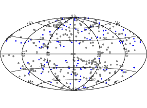
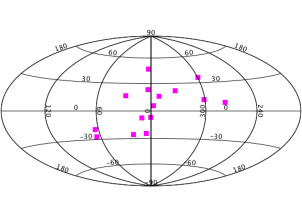
Figure 1: Top panel: Hammer-Aitoff projection in galactic coordinates of the sky distribution for the sample of 397 Galactic field RRLs and the subsample of 291 RRLs with ruwe $<$ 1.4 ( blue and grey symbols in the upper plot, respectively). Bottom panel: The 15 globular clusters (magenta symbols, lower plot) hosting the RRLs considered in the present study.

Table 1: Properties of 15 Galactic GCs used in this study.

Cluster ID	$E(B-V)$	AV	$\rm[Fe/H]$	$\mu_{V}$	distance	RRLs∗
	(mag)	(mag)	(dex)	(mag)	(kpc)
NGC 3201	0.220 $\pm$ 0.015	0.682	$-$1.51 $\pm$ 0.02	14.20	4.9	86
NGC 4590 (M68)	0.053 $\pm$ 0.001	0.162	$-$2.27 $\pm$ 0.04	15.21	10.3	42
NGC 5824	0.148 $\pm$ 0.003	0.454	$-$1.94 $\pm$ 0.14	17.94	32.1	48
NGC 5904 (M5)	0.032 $\pm$ 0.001	0.097	$-$1.33 $\pm$ 0.02	14.46	7.5	129
NGC 6121 (M4)	0.428 $\pm$ 0.150	1.549	$-$1.18 $\pm$ 0.02	12.82	2.2	47
NGC 6171 (M107)	0.395 $\pm$ 0.006	1.264	$-$1.03 $\pm$ 0.02	15.01	6.4	23
NGC 6316	0.653 $\pm$ 0.031	2.089	$-$0.36$\pm$ 0.14	16.77	10.4	2
NGC 6426	0.298 $\pm$ 0.012	0.934	$-$2.39 $\pm$ 0.30	17.68	20.6	16
NGC 6569	0.369$\pm$0.008	1.181	$-$0.72$\pm$ 0.14	16.83	10.9	21
NGC 6656 (M22)	0.280 $\pm$ 0.100	0.896	$-$1.70 $\pm$ 0.08	13.60	3.2	31
NGC 6864 (M75)	0.130 $\pm$ 0.004	0.403	$-$1.29 $\pm$ 0.14	17.09	20.9	41
NGC 7006	0.071 $\pm$ 0.004	0.214	$-$1.46 $\pm$ 0.06	18.23	41.2	64
NGC 7078 (M15)	0.093 $\pm$ 0.003	0.291	$-$2.33 $\pm$ 0.02	15.39	10.4	143
Rup 106	0.150 $\pm$ 0.003	0.458	$-$1.78 $\pm$ 0.08	17.25	21.2	13
Ter 8	0.127 $\pm$ 0.003	0.392	$-$2.06 $\pm$ 0.30	17.47	26.3	3
NOTES. $E(B-V)$ values are from Schlafly & Finkbeiner (2011). See text for details.
Spectroscopic metallicities from Carretta et al. (2009) and Dias et al. (2016) on Carretta et al. (2009) scale.
The $\mu_{V}$ and distance values are from Harris (1996, version 2010).
∗ Number of RRLs known. References:
NGC 3201 (Layden & Sarajedini, 2003; Arellano Ferro et al., 2014), NGC 4590 (Kains et al., 2015),
NGC 5824 (Walker et al., 2017), NGC 5904 (Oosterhoff, 1941; Kaluzny et al., 2000; Arellano Ferro et al., 2016),
NGC 6121 (Yao et al., 1988; Kaluzny et al., 2013; Stetson et al., 2014),
NGC 6171 (Dickens, 1970; Clement & Shelton, 1997; Samus et al., 2009; Drake et al., 2013), NGC 6316 (Layden et al., 2003),
NGC 6426 (Grubissich, 1958; Papadakis et al., 2000; Samus et al., 2009), NGC 6569 (Hazen-Liller, 1985; Soszyński et al., 2014)   ,
NGC 6656 (Kunder et al., 2013; Soszyński et al., 2014),
NGC 6864 (Corwin et al., 2003; Scott et al., 2006), NGC 7006 (Wehlau et al., 1999; Samus et al., 2009),
NGC 7078 (Corwin et al., 2008), Rup 106 (Kaluzny et al., 1995), Ter 8 (Salinas et al., 2005; Torrealba et al., 2015)

In this section we present the two separate data samples: RRLs in the MW field and in Galactic GCs used for the derivation of the corresponding $LZ$ relations in the $V$ and $G$ passbands and $PWZ$ relations in the Gaia $G$, $G_{\rm BP}$ and $G_{\rm RP}$ bands.

2.1 Field RR Lyrae stars

We have built our field RRL sample starting from the 401 MW RRLs analysed in Muraveva et al. (2018) which were based on the Dambis et al. (2013) sample. We first replaced their Gaia DR2 parallaxes with the new EDR3 values ($\varpi_{EDR3}$), which are available for the whole sample. We then discarded stars DI Leo and VX Ind because they were re-classified by Ripepi et al. (2019) as a classical Cepheid and a Population II Cepheid of BL Herculis type, respectively. We also excluded CK UMa, because the star lacks a spectroscopic metallicity estimate, and V363 Cas that Dambis et al. (2013) classifies as fundamental mode RRL (RRab) but it is in fact a Galactic classical Cepheid according to the literature (Ripepi et al. 2019 and references therein). The RRLs in our sample have parallaxes ranging from $-$0.05 mas to 3.98 mas, with only three of them having a negative parallax. We note that our MW field sample includes RR Lyr itself, the bright variable star after which the whole class is named. Unlike in Gaia DR2, the EDR3 parallax of RR Lyr has a positive and reliable value of $3.98\pm 0.03$ mas, which is in good agreement with the Gaia DR1 and the Hubble Space Telescope (HST) estimates (see Gaia Collaboration et al., 2017, table 1). Our sample thus includes 397 MW RRLs homogeneously distributed all over the sky (filled circles in the upper panel of Fig. 1). Uncertainties of the Gaia EDR3 parallaxes for the 397 RRLs in our sample are shown by the blue histogram in Fig 2. They range from 0.01 to 0.20 mas. For comparison, the green histogram shows the error distribution of the DR2 parallaxes of these RRLs.
To restrict the sample of field RRLs used to calibrate the $LZ$ and $PLZ$ relations only to sources with best quality parallaxes we took into account the re-normalised unit weight error (ruwe) (Lindegren, 2018) and retained only sources satisfying the condition ruwe < 1.4. With this selection the sample is reduced to 291 stars (73$\%$; grey filled circles in the upper plot of Fig. 1), 260 of which are fundamental mode (RRab) and 31 are first-overtone (RRc) pulsators. The distribution of the parallax uncertainties for these 291 RRLs is shown by the grey histogram in the top panel of Fig 2. We provide information for the complete dataset of 291 MW field RRLs in Table 10. For each RRL we list the literature name (column 1), pulsation mode and period (columns 7 and 8), mean apparent magnitude in the $V$-band $\langle V\rangle$ (column 9), absorption in $V$-band (column 11) and metallicity estimation in the Zinn & West (1984) metallicity scale (column 19), taken from table 1 of Muraveva et al. (2018). In addition we include the Gaia EDR3 source identifier (column 2), the EDR3 coordinates (columns 3 and 4), the EDR3 parallax and its error (columns 5 and 6), and the intensity-averaged mean magnitudes in the $\langle G\rangle$, $\langle G_{\rm{BP}}\rangle$ and $\langle G_{\rm{RP}}\rangle$ bands and their respective errors taken from the Gaia DR2 vari_rrlyrae table (Clementini et al., 2019). To derive the $M_{V}-\rm[Fe/H]$ and $M_{G}-\rm[Fe/H]$ relations, among the 291 field RRLs, we have used 274 sources having $V$ magnitude (see Section 4.2) and 223 sources with $G$ magnitude (see Section 4.3), respectively. A subsample of 190 field RRLs having $\langle G\rangle$, $\langle G_{\rm{BP}}\rangle$ and $\langle G_{\rm{RP}}\rangle$ magnitudes were instead used to infer the $PW_{\left(G,G_{\rm{BP}},G_{\rm{RP}}\right)}Z$ relation (see Section 4.4).

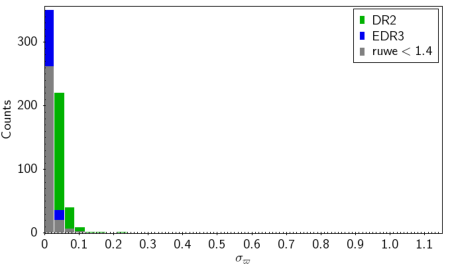
Figure 2: Top panel: The blue histogram shows the distribution of the EDR3 parallax uncertainties ($\sigma_{\varpi_{EDR3}}$) for our initial sample of 397 field RRLs. For comparison the DR2 parallax uncertainties of the stars are represented by a green histogram. The grey histogram shows the $\sigma_{\varpi_{EDR3}}$ distribution for the subsample of 291 RRLs with ruwe<1.4. Bottom panel: The magenta histogram shows the distribution of the EDR3 parallax uncertainties for our initial sample of 582 RRLs in GCs. The grey histogram shows the $\sigma_{\varpi_{EDR3}}$ distribution for the subsample of 385 GC RRLs with ruwe<1.4. In both panels the bin size is 0.03 mas.

2.2 RR Lyrae stars in Globular Clusters

We selected a sample of 15 Galactic GCs with distances ranging from a few to $\sim$ 41 kpc around the Galactic centre and spatially distributed as shown in the bottom panel of Fig. 1. The 15 GCs cover a large range in metal abundance, from $-$2.39 to $-$0.36 dex in [Fe/H]. Their $V$ luminosity at the horizontal branch (HB) level spans about 5 magnitudes, going from 13.30 mag for NGC 6121 to 18.80 mag for NGC 7006 (Harris, 1996).

According to the literature, the selected GCs host a total number of 709 RRLs. For each of the 15 GCs we list in Table  1 reddening value $E(B-V)$ (taken from Schlafly & Finkbeiner 2011 using as reference the GC centers), absorption in the $V$-band, spectroscopic metallicity (in the Carretta et al. 2009 scale) from Dias et al. (2016), visual distance modulus and distance (in kpc) from Harris (1996) catalogue .
In the last column of Table 1 we also give the number of RRLs in each cluster. References to the papers used to collect the samples of GC RRLs are provided in the table notes. We cross-matched the 709 cluster RRLs against the Gaia EDR3 catalogue using a cross-match radius of 2 arcseconds and retained only sources unambiguously classified by the literature as fundamental and first-overtone RRLs, including also those exhibiting the Blazhko effect (Blažko 1907; labels “RRAB”, “RRAB Bl”, “RRC" and “RRC Bl”). With this filtering the GC RRL sample reduced to 643 sources. We then dropped 3 sources with unknown period and further 58 RRLs for which a parallax is not available in the Gaia EDR3 catalogue, thus remaining with a total sample of 582 GC RRLs (372 RRab and 210 RRc stars). Finally, as done for the field RRLs we cleaned the GC RRLs discarding sources with ruwe $\geq 1.4$. With this latter filtering the sample was reduced to 385 stars (66$\%$, 249 RRab and 136 RRc stars). The distributions of the EDR3 parallax uncertainties for the 582 and 385 GC RRL samples are shown by the magenta and grey histograms in Fig. 2, respectively. The complete dataset with the relevant information (sourceids, coordinates, parallax and parallax errors from EDR3, pulsation mode, period, $\langle V\rangle$, and DR2 $\langle G\rangle$ ,$\langle G_{\rm{BP}}\rangle$, $\langle G_{\rm{RP}}\rangle$ mean magnitudes) is summarised in Table 11.

To compute the $LZ$ and $PW$ relations our Bayesian method (see Section 3 below) corrects the mean apparent magnitudes of the GC RRLs using the $V$-absorption values provided for each GC in columns 3 of Table 1, which are taken from Schlafly & Finkbeiner (2011) assuming a standard total-to-selective absorption ($R_{V}=$3.1). Five GCs of our sample, which are located closer to the center of the Galaxy, are Bulge systems. They are heavily affected by extinction and have a higher metal content. Different studies (Barbuy et al. 1998; Bica et al. 2016 and references therein) have measured a total-to-selective absorption for these GCs higher than 3.1. For NGC 6171, NGC 6316, NGC 6656 and NGC 6569 we converted $E(B-V)$ into $A_{V}$ using $R_{V}=$3.2 as proposed by Bica et al. (2016) while for NGC 6121 we adopted $R_{V}=$3.62 as found by Hendricks et al. (2012). We assumed that in each GC the absorption is constant with the exclusion of NGC 6121 and NGC 6569 which are known to be severely affected by differential reddening. For them, we estimated the $E(B-V)$ reddening and its uncertainty individually for each RRL. In particular, we adopted as reddening zero-points the values of Schlafly & Finkbeiner (2011) measured at the NGC 6121 and NGC 6569 centres and derived individual $E(B-V)$ values for each RRL in these clusters using their differential reddening maps provided by Alonso-García et al. (2012).
Contrary to the field RRLs, the RRLs in our GC sample lack individual and homogeneous metal abundance estimations. Hence, on the assumption that the clusters considered in our study are mono-metallic, we assigned to their RRLs the spectroscopic metal abundances (on the Carretta et al. 2009 scale) derived for the host clusters by Dias et al. (2016) and listed in column 4 of Table 1.

Figure 3 shows the EDR3 proper motions (top panels), the spatial distributions (middle panels) and the $G,G_{\rm BP}-G_{\rm RP}$ colour-magnitude diagrams (bottom panels) for two GCs in our sample, namely: NGC 4590 (left panels) and NGC 6121 (right panels). We have marked with blue dots the GC RRLs observed by Gaia that we used in our analysis.

We adopted the literature period for all cluster RRLs except for V27 in NGC 5824. Walker et al. (2017) reports this RRL to have a noisy light curve perhaps due to an incorrect period. We thus adopted for the star the period provided by the Gaia DR2 vary-rrlyrae table. Periods of all RRc stars (31 sources among the field RRLs and 136 sources among the cluster RRLs) were “fundamentalised” by adding 0.127 to the decadic logarithm of the period and uncertainties on $\log\left(P\right)$ were estimated as $\sigma_{\log\left(P\right)}=0.01$, which is equivalent to an uncertainty of 2.3% in the period. This choice, rather conservative, to apply a large error to the periods is due both to the frequent absence in the literature of period uncertainties and to the heterogeneity of the values measured in different works.

V75 in NGC 6121 (Gaia sourceid 6045480963805292416) was removed from our sample of 385 cluster RRLs because the mean $V$ magnitude reported for the star by Yao et al. (1988) is almost 1 mag fainter than for the other RRLs in the cluster while in a more recent work of Stetson et al. (2014) its luminosity is considerably brighter than the others likely due to limitations of its time sampling. After removing also 18 sources for which a $V$ magnitude is not available in the literature, or the V-mean magnitude coming from literature is not so accurate [as V34 in NGC 6121, for this star Stetson et al. (2014) had insufficient data to fit the light curve], the sample of cluster RRLs reduced to 366 sources that we used to infer the $M_{V}-{\rm[Fe/H]}$ relation presented in Section 4.2. As for the $LZ$ relation in the $G$-band, after dropping sources without a $\langle G\rangle$ magnitude in the DR2 vary-rrlyrae table, the final sample used to define the $M_{G}-{\rm[Fe/H]}$ relation consisted of 227 cluster RRLs (Section 4.3). $\langle G_{\rm{BP}}\rangle$ and $\langle G_{\rm{RP}}\rangle$ mean magnitudes are available for a subsample of 168 cluster RRLs. They were used to compute the $PW_{\left(G,G_{\rm{BP}},G_{\rm{RP}}\right)}$ relations described in Section 4.4. The $G$-band absorption was estimated from the absorption in the $V$-band using the relation: ${A}_{G}=0.840{A}_{V}$ (Bono et al., 2019).

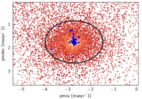
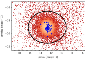
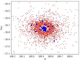
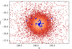
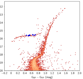
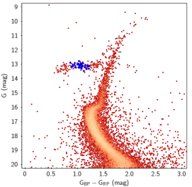
Figure 3: Proper motions (top), spatial distribution (middle) and $G$, $G_{\rm BP}-G_{\rm RP}$ colour-magnitude diagram (CMD; bottom) of two GCs in our sample: NGC 4590 (${\rm[Fe/H]}=-$2.27; left) and NGC 6121 (${\rm[Fe/H]}=-$1.18; right). The CMDs are drawn using for constant stars magnitudes from the EDR3 catalogue. Black ellipses in the top panels encircle stars plotted in the CMDs in the bottom panels of the figure. Blue dots show the cluster RRLs (42 RRLs in the top and middle panels and 13 RRLs with mean $G$, $G_{\rm BP}$ and $G_{\rm RP}$ magnitudes from the Gaia DR2 vari_rrlyrae table, in the CMD of NGC4590; 47 RRLs in the top and middle panels and 37 RRLs in the CMD of NGC 6121).

3 Method

In this section we summarise the fundamentals of the hierarchical Bayesian method and describe the model we developed for inferring $PL(Z)$ relations from our sample of GC RRLs. The hierarchical model for inferring $PL(Z)$ relations for field RRLs used in this paper is essentially the same as described in section 4 of Muraveva et al. (2018). The only difference is the treatment of the parallax offset. While in the model of Muraveva et al. (2018) we included a unique offset, namely a global parallax zero-point offset, we now allow the offset to vary for each source in the sample. The RRLs in our samples are distributed all-sky covering a quite wide range in G-magnitude with different extinction values and crowding conditions. Since all these factors affect the zero-point offset we have decided to adopt a varying offset to minimize these effects. But as reported in Section 4.1 below, the model with a unique offset is still used to get an initial guess of the global offset value, which is then set as prior information in the models with varying offset.

The hierarchical Bayesian method starts by partitioning the parameter space associated to the problem into several hierarchical levels of statistical variability. This partition applies, in the most general case, both to the parameters themselves (random variables) and to the measurements (data). In a further stage the modelling process assigns a set of probabilistic conditional dependency relationships between parameters and data, at the same or different level of the hierarchy. The final result is a model for the problem expressed as the joint probability density function (PDF) of parameters and measurements factorized as the product of a set of conditional probability distributions, namely a Bayesian network (Pearl, 1988; Lauritzen, 1996). Assuming that the data are partitioned into $J$ clusters with $N_{j}$ sets of measurements in each (one for each individual star) from a total of $N=\sum_{j=1}^{J}N_{j}$ stars, and that the random parameters are partitioned into true astrophysical parameters ($\Theta$) and hyperparameters ($\Phi$), we express the network as

$$\begin{split}p\left(\mathcal{D},\mathbf{\Theta},\Phi\right)=&\prod_{j=1}^{J}p\left(\mathbf{d}_{j}\mid\mathbf{\Theta}_{j}\right)\cdot\prod_{i=1}^{N_{j}}p\left(\mathbf{d}_{ij}\mid\mathbf{\Theta}_{ij}\right)\cdot\\ &p\left(\mathbf{\Theta}\mid\Phi\right)\cdot p\left(\Phi\right)\,,\\ \end{split}$$ (1)

where $\mathbf{d}_{ij}$ are the observational data of star $i$ in cluster $j$ (apparent magnitudes, parallaxes and periods as explained below), ${\mathbf{d}}_{j}$ represent the observations pertaining to cluster $j$ (its metallicity assumed to be the same for all stars in the cluster) and $\mathcal{D}=\left\{\mathbf{d}_{j},\mathcal{D}_{j}\right\}_{j=1}^{J}$, with $\mathcal{D}_{j}=\left\{\mathbf{d}_{ij}\right\}_{i=1}^{N_{j}}$. The astrophysical parameters denoted by $\mathbf{\Theta}_{ij}$ in Eq. (1) include the true distance, true period and absolute magnitude associated to each RRL in every GC, while the parameters denoted by $\mathbf{\Theta}_{j}$ include the true metallicity, the coefficients of the $PL$ relationship and the parameters characterizing the GC spatial distribution associated to each GC. The hyperparameters $\Phi$ include the coefficients of the global $PLZ$ relation. The first two products on the right hand side of Eq. (1) constitute the conditional distribution of the data given the parameters (the so called likelihood), $p\left(\mathbf{\Theta}\mid\Phi\right)$ is the prior distribution of the true parameters given the hyperparameters and $p\left(\Phi\right)$ is the unconditional hyperprior distribution of the hyperparameters. A model like the one described in Eq. (1) dictates a certain dependency structure between variables which is formally expressed by a directed acyclic graph (DAG) whose nodes encode model parameters, measurements, or constants, and whose directed links represent conditional dependence relationships. While Eq. (1), and the associated DAG in particular, represent the problem formulation, the solution is based on the application of Bayes’ rule:

$$p\left(\mathbf{\Theta},\Phi\mid\mathcal{D}\right)\propto p\left(\mathcal{D}\mid\mathbf{\Theta}\right)\cdot p\left(\mathbf{\Theta}\mid\Phi\right)\cdot p\left(\Phi\right)\,,$$ (2)

being the goal to infer the marginal posterior distribution $p\left(\Lambda\mid\mathcal{D}\right)$ of some subset [$\Lambda\subseteq\left(\mathbf{\Theta},\Phi\right)$] of the parameters of interest. For multi-level models with a relatively complex dependency structure between their parameters, the posterior distribution usually is not available in an analytically tractable closed form but can be evaluated using Markov chain Monte Carlo (MCMC) simulation techniques.

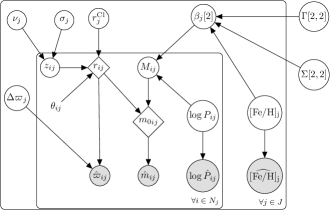
Figure 4: Directed Acyclic Graph (DAG) that represents the generic hierarchical Bayesian model (HBM) used to infer the coefficients of the $PL$, $LZ$ and $PLZ$ relations. A full description of the model parameters is included in the text.

In what follows we describe the construction of the hierarchical probabilistic graphical model (abbreviated hereafter as HM) applied in this paper to the inference of $PL(Z)$ relations for RRLs in GCs. Figure 4 shows its associated DAG representing the conditional dependence relationships between the parameters and data. Parameters and data are represented by DAG nodes enclosed into two nested rectangles (plate notation) to make evident the grouped nature of the problem. The nodes located into the outer plate but not into the inner plate represent properties at a GC level like the cluster mean iron-to-hydrogen content and the coefficients of an underlying $PL$ relationship for the population of RRLs in the cluster. The outer plate replicates in the DAG as many times ($J$) as the total number of clusters (groups), with the subindex $j$ identifying a particular cluster. The nodes placed into the inner plate represent properties of individual stars (e.g. the time averaged absolute magnitude $M$). For the $j$th cluster, the inner plate replicates as many times ($N_{j}$) as the size of the cluster RRL sample, with the subindex $i$ identifying a particular star.

Figure 4 shows the measurements as shaded nodes at the bottom of the DAG. At the individual star level (inner plate) these measurements are the decadic logarithm of period $\log\hat{P}_{ij}$, the apparent magnitude $\hat{m}_{ij}$ and the parallax $\hat{\varpi}_{ij}$. At the cluster level (outer plate) the only measurement is the GC mean iron-to-hydrogen content $\widehat{\left[\mathrm{Fe/H}\right]}_{j}$. Quantities that are considered constant in the model are not represented in the DAG. These quantities include all the measurement uncertainties, the measured interstellar absorption $\hat{A}_{m_{ij}}$ and all the model hyperprior parameters (for example the parameter values used to define the hyperprior for the distance to the centre of each GC). The measurements are assumed to be realizations from Gaussian distributions centred at their true (unknown) values (this is only an approximation in the case of the apparent magnitudes; only the uncertainties in the measured fluxes are Gaussian), which are represented without the circumflex accent (^) in the DAG. The adopted standard deviations are the measurement uncertainties provided by our catalogue. In the particular case of the parallax, we assume that its true value is equal to the reciprocal of the true distance and contemplate the possibility that its measured value may be affected by a parallax offset which varies with the globular cluster. This is formulated as

$$\hat{\varpi}_{ij}\sim\mathcal{N}\left(\frac{1}{r_{ij}}+{\Delta\varpi}_{j},\sigma_{\varpi_{ij}}\right)\,,$$ (3)

where $\sim$ should be read as ’is distributed as’, $\mathcal{N}$ represents the normal (Gaussian) distribution, $r_{ij}$ is the true distance to the star and ${\Delta\varpi}_{j}$ is the parallax offset associated to the $j$th GC. The parallax offsets are given as a Gaussian prior centred at the value (mas) inferred by the field stars HM described in section 4 of Muraveva et al. (2018) applied to the inference of a $PW_{(G,G_{\rm BP},G_{\rm RP})}Z$ relation (the details of that inference are given in Section 4.1 further below). The standard deviation that accounts for the offset variability between clusters is fixed at a value of $0.03$ mas. This value, which is about an order of magnitude larger than the standard deviation obtained from the preliminary calibration of relations for field RRLs, takes into account the large uncertainties of the parallax measurements of RRLs in the GC sample. The Heliocentric distances $r_{ij}$ are modeled as a function of the distance to the centre of each cluster assuming that the cluster geometry is spherical as explained at the end of the section. The measured apparent magnitude $\hat{m}_{ij}$ of the $i$th star belonging to the $j$th globular cluster is modelled by a Gaussian distribution centred at its true value ${m_{0}}_{ij}$, while the true value is generated deterministically as

$${m_{0}}_{ij}=M_{ij}+\hat{A}_{m_{ij}}+5\log(r_{ij})+10\,,$$ (4)

where $M_{ij}$, $\hat{A}_{m_{ij}}$, and $r_{ij}$ denote the true absolute magnitude, the measured interstellar absorption and the true distance (kpc), respectively. For each globular cluster the model contemplates a different $PL$ relationship which is parameterized as

$$M_{ij}\sim\mathcal{N}\left(\left(\begin{array}[]{cc}\beta_{0j}&\beta_{1j}\end{array}\right)\cdot\left(\begin{array}[]{c}1\\ \log P_{ij}\end{array}\right),\sigma_{j}\right)\,.$$ (5)

The coefficients of the $PL$ relations are assigned a bivariate Normal prior in turn, whose mean vector depends on the true metallicity of the globular cluster in the most general case:

$$\left(\begin{array}[]{c}\beta_{0j}\\ \beta_{1j}\end{array}\right)\sim\mathcal{N}\left(\left(\begin{array}[]{cc}\gamma_{00}&\gamma_{01}\\ \gamma_{10}&\gamma_{11}\end{array}\right)\cdot\left(\begin{array}[]{c}1\\ \left[\mathrm{Fe/H}\right]_{j}\end{array}\right),\Sigma\right)\,,$$ (6)

where $\Sigma=\mathrm{diag}\left({\tau}_{\beta_{0}}^{2},{\tau}_{\beta_{1}}^{2}\right)$ and the standard deviations $\tau_{\beta_{\cdot}}$ are drawn from an exponential prior with inverse-scale parameter equal to 1. For the slopes $\gamma_{\cdot 1}$ and zero-points $\gamma_{\cdot 0}$ population-level parameters we specify standard Cauchy prior distributions centred at 0 with scale parameter equal to 1 and 10, respectively.

We emphasize that the metallicities enter the model in an upper hierarchical level than periods, something made explicit in the DAG depicted in Fig. 4 where the $N_{j}$ RRL stars of the $j$th cluster are all inside the inner plate but $\left[\mathrm{Fe/H}\right]$ is placed into the outer plate. The model assumes that all the RRLs of a given globular cluster have the same metallicity and that the slope ($\beta_{1j}$) and intercept ($\beta_{0j}$) of the PL relation depend on the cluster metallicity $\left[\mathrm{Fe/H}\right]_{j}$. The method contemplates the possibility of modelling the influence of the cluster metallicity only on the intercept of the $PL$ relations which would be implemented by setting $\gamma_{11}=0$. For a model that does not take into account the influence of the pulsation period, namely a $LZ$ relationship, Eqs. 5 and 6 particularise to

$$M_{ij}\sim\mathcal{N}\left(\beta_{0j},\sigma_{j}\right)$$ (7)

and

$$\beta_{0j}\sim\mathcal{N}\left(\gamma_{00}+\gamma_{01}\left[\mathrm{Fe/H}\right]_{j},\tau\right)\,,$$ (8)

respectively.

The Bayesian method proposed in this paper constrains the $PL(Z)$ relations by modelling explicitly the spatial distribution of the RR Lyrae star population of each globular cluster in our sample. The GC spatial distribution is assumed to be spherical. We define two reference frames: one centred at the solar system barycentre. In this reference system the distance to the $j$th cluster centre is defined as $r_{j}$ and the distance to the $i$th star in this $j$th cluster as $r_{ij}$. The second reference system has its origin at the cluster centre and the $z$-axis pointing towards the observer. We assume that the 3D probability distribution of the coordinates of RR Lyrae stars in this reference system is given by the product of three independent non-standardized Student’s $t$-distributions, one for each Cartesian component, with identical degrees of freedom $\nu_{j}$ and scale parameter $\sigma_{j}$ (see below for a justification of this choice). In particular, the non-standardized Student’s t probability density function (PDF) corresponding to the coordinate $z_{ij}$ of a source (which in the adopted reference frame represents the projection of the radial distance from the source to the cluster centre onto the line of sight) is given by

$$f\left(z_{ij}\right)=\frac{1}{\sqrt{\nu_{j}\sigma_{j}^{2}}\mathrm{B}\left(\nu_{j},\frac{1}{2}\right)}\left(1+\frac{z_{ij}^{2}}{\nu_{j}s_{j}^{2}}\right)^{-\frac{\nu_{j}+1}{2}}\,,$$ (9)

where B denotes the Beta function. We note that through the reparameterisation $s_{j}=\sqrt{\nu_{j}\sigma_{j}}$ and $m_{j}=\frac{\nu_{j}+1}{2}$ the PDF of Eq. (9) is equivalent to the so called generalized Schuster density (Ninkovic, 1998) with the parameters $s_{j}$ and $m_{j}$ representing the cluster core length scale and the steepness of the $j$th GC stellar distribution, respectively, which for $m=\frac{3}{2}$ approximates the King stellar surface density profile (Ninkovic, 1998). While the parameters $\sigma_{j}$ and $\nu_{j}$ are directly inferred by our HM, $s_{j}$ and $m_{j}$ are calculated deterministically from the former. Our HM assigns for $\sigma_{j}$ and $\nu_{j}$ an exponential prior with inverse scale $\lambda=50$ $\mathrm{kpc}^{-1}$ and an exponential prior shifted $2$ units towards positive values with inverse scale $\lambda=1$, respectively.

The value of the barycentric distance $r_{ij}$ to the $i$th RR Lyrae star of the $j$th cluster is calculated deterministically from its $z_{ij}$ coordinate, the barycentric distance to the cluster centre $r_{j}^{\mathrm{Cl}}$ and the angular separation $\theta_{ij}$ between the star and the cluster centre by

$$r_{ij}=\frac{r_{j}^{\mathrm{Cl}}+z_{ij}}{\cos\left(\theta_{ij}\right)}\,,$$ (10)

where the angular distances $\theta_{ij}$ are kept constant in the model and calculated from

$$\begin{split}\cos\left(\theta_{ij}\right)=&\cos\left(\frac{\pi}{2}-\delta_{ij}\right)\cos\left(\frac{\pi}{2}-\delta_{j}^{\mathrm{Cl}}\right)+\\ &\sin\left(\frac{\pi}{2}-\delta_{ij}\right)\sin\left(\frac{\pi}{2}-\delta_{j}^{\mathrm{Cl}}\right)\cos\left(\alpha-\alpha_{j}^{\mathrm{Cl}}\right).\\ \end{split}$$ (11)

In Eq. (11), $\alpha_{j}^{\mathrm{Cl}}$, $\delta_{j}^{\mathrm{Cl}}$, $\alpha_{ij}$ and $\delta_{ij}$ are the right ascension and declination of the cluster centre and the individual RR Lyrae stars, respectively. The distance $r_{j}^{\mathrm{Cl}}$ to each cluster centre is assigned a Gamma prior distribution with shape $k=2$ and scale parameter $L$ equal to the distance to the cluster provided by Harris (1996, 2010 edition).

We have encoded our HM in the Stan probabilistic modelling language (Carpenter et al., 2017) and sampled the model posterior distribution by means of the adaptive Hamiltonian Monte Carlo (HMC) No-U-Turn Sampler (NUTS) of Hoffman & Gelman (2014) through the use of the R (R Core Team, 2017) interface Rstan (Stan Development Team, 2018).

4 Results

4.1 Gaia  EDR3 parallax offset

To obtain an independent estimate of the Gaia  EDR3 parallax offset distribution (see e.g. Lindegren et al., 2020; Bhardwaj et al., 2020; Zinn, 2021; Stassun & Torres, 2021, among others) we used a two-stage procedure. In the first stage we applied the HM described in section 4 of Muraveva et al. (2018) for calibrating a preliminary $PW_{(G,G_{\rm BP},G_{\rm RP})}Z$ relation (using our field RRL sample) and inferring the associated global parallax offset parameter included in the model. In this first stage we assigned the offset a weakly informative Gaussian prior centred at $\mu_{\varpi_{0}}=0$ mas with standard deviation $\sigma_{\varpi_{0}}=0.1$ mas and inferred the posterior credible interval $\Delta_{\varpi_{0}}=-0.033_{-0.006}^{+0.005}$ mas, defined here, and hereinafter, as the median plus/minus the difference in absolute value between the median and the 84th and 16th percentile of the posterior distribution of the parameter. Then, in the second stage, we adopted a Gaussian prior distribution centred at ${\mu_{\varpi_{0}}}_{j}=-0.033$ mas with ${\sigma_{\varpi_{0}}}_{j}=0.03$ mas for the individual offsets of the GC and field RRL models described in Section 3, based on the offset inferred in our first stage. The results of this second stage are reported in the following sections. We use the HM with individual parallax offset to allow the offset to vary with the sky position (among other factors). For that we could have proceeded directly in a single step by using the weakly informative Gaussian prior centred at 0 mas. However, this results in a largely unconstrained model space, poor convergence and unphysical posterior distributions due to the significant fractional uncertainties of the parallax measurements in our sample.

4.2 $M_{V}-{\rm[Fe/H]}$ relation

The statistical results of the $M_{V}-{\rm[Fe/H]}$ relation parameters inferred by our HM at GC level for our selection of 366 cluster RRLs in the $V$ band are presented in Table 2. Each parameter is summarised by the median plus minus the difference in absolute value between the median and the 84th and 16th percentile of its posterior distribution, as defined in Section 4.1. The table includes: the parameter $\beta_{0j}$ of Eq. 7 representing the mean absolute magnitude (zero-point) of each GC RRL star population ($M_{j}$), the intrinsic dispersions $\sigma_{j}$ (Eq. 7) of the individual RRL absolute magnitudes around the GC mean absolute magnitude (${\sigma_{M}}_{j}$), the true distance modulus of each GC ($\mu_{j}$) calculated deterministically from the inferred barycentric distance to the GC centre ($r_{j}^{\rm Cl}$), the median projections of the radial distances from each source to the GC centre onto the line of sight (${z_{\cdot j}}$) and the cluster-level parallax offsets inferred by our HM (${\Delta\varpi}_{j}$).

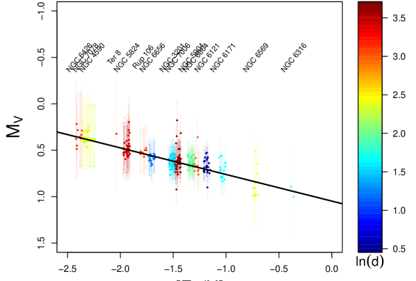
Figure 5: $M_{V}-{\rm[Fe/H]}$ relation defined by globular cluster RRLs as summarized in Table 2. The solid line represents the linear fit corresponding to the parameters of Table 3. The colour scale encodes the (natural) logarithm of the inferred (true) barycentric distance to individual RRL stars measured in units of kpc.

The upper portion of Table 3 summarises the results of the inference at the top (population-level) of our HM. It reports the slope, zero-point and intrinsic dispersion obtained for the $M_{V}-{\rm[Fe/H]}$ relation, and the inferred population-level parallax zero-point offset ${{\Delta\varpi}_{0}=-0.024_{-0.008}^{+0.008}}$ mas calculated as the median of the distribution of the medians of each sample of the joint posterior distribution of ${\Delta\varpi}_{j}$. Figure 5 shows the corresponding fit. The credible intervals obtained for the metallicity slope and the intercept are ${\gamma_{1}^{\rm UVES}=0.29_{-0.29}^{+0.35}}$ mag/dex and ${\gamma_{0}^{\rm UVES}=1.05_{-0.46}^{+0.43}}$ mag, respectively, with an associated intrinsic dispersion of ${\sigma_{M}=0.11_{-0.08}^{+0.15}}$ mag. Our inferred GC $M_{V}-{\rm[Fe/H]}$ relation for metal abundances on the Carretta et al. (2009) metallicity scale is then given by

$$M_{V}=\left(0.29_{-0.29}^{+0.35}\right)\left[\mathrm{Fe/H}\right]+\left(1.05_{-0.46}^{+0.43}\right)\,.$$ (12)

We recall that these results correspond to an inferred global parallax offset ${{\Delta\varpi}_{0}=-0.024_{-0.008}^{+0.008}}$ mas calculated as explained above.

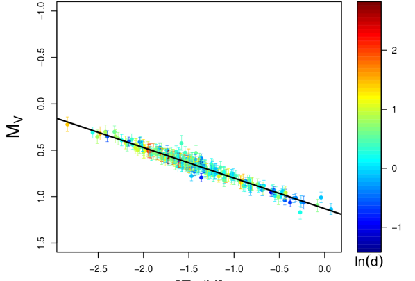
Figure 6: $M_{V}-{\rm[Fe/H]}$ relation defined by our field RRL sample. The solid line represents the linear fit corresponding to the parameters of Table 3. The colour scale encodes the (natural) logarithm of the inferred (true) barycentric distance to individual RRL stars measured in units of kpc.

In Table 3 (lower portion) and Fig. 6 we present the results of our updated Bayesian analysis using Gaia  EDR3 parallaxes applied to the sample of the 274 field RRLs that satisfy the criterion ruwe < 1.4 for which the $V$ magnitude was available. The credible intervals obtained for the metallicity slope and the intercept are $\gamma_{1}^{\rm ZW}=0.33_{-0.02}^{+0.02}$ mag/dex and $\gamma_{0}^{\rm ZW}=1.13_{-0.03}^{+0.02}$ mag, respectively, with an associated intrinsic dispersion of $\sigma_{M}=0.02_{-0.01}^{+0.01}$ mag. Our inferred $M_{V}-{\rm[Fe/H]}$ relation for field stars with metal abundances on the Zinn & West (1984) metallicity scale is then given by

$$M_{V}=\left(0.33_{-0.02}^{+0.02}\right)\left[\mathrm{Fe/H}\right]+\left(1.13_{-0.03}^{+0.02}\right)\,.$$ (13)

For the $M_{V}-{\rm[Fe/H]}$ relation for field stars we report the parallax zero-point offset ${\Delta\varpi}_{0}=-0.033_{-0.002}^{+0.002}$ mas (Table 3, last column of the lower portion) calculated as the median of the distribution of the medians of each sample of the joint posterior distribution of the parallax offsets inferred by our HM for the field RRLs in the sample.

To compare the relation for cluster RRLs, Eq. (12), with the field RRL $M_{V}-{\rm[Fe/H]}$ relation of Eq. (13) we have to account for the difference between the metallicity scales of the two samples. From the linear relation

$$\left[\mathrm{Fe/H}\right]_{\mathrm{UVES}}=1.105\left[\mathrm{Fe/H}\right]_{\mathrm{ZW}}+0.160$$ (14)

of Carretta et al. (2009) we obtain that the relationship between the slopes and intercepts in the Zinn & West (1984) and Carretta et al. (2009) metallicity scales is given by

$$\gamma_{1}^{\mathrm{ZW}}=1.105\gamma_{1}^{\mathrm{UVES}}$$ (15)

and

$$\gamma_{0}^{\mathrm{ZW}}=0.160\gamma_{1}^{\mathrm{UVES}}+\gamma_{0}^{\mathrm{UVES}}\,,$$ (16)

respectively, where we use the superscript UVES to refer to the mean GC iron abundance ([Fe/H]) derived from high resolution spectra of red giant branch (RGB) stars obtained with the Ultraviolet and Visual Echelle Spectrograph (UVES) using the procedure described in Carretta et al. (2009, and references therein). Applying the former conversion to the inferred slope of Table 3 we obtain ${\gamma_{1}^{\rm ZW(UVES)}=0.32_{-0.32}^{+0.39}}$ mag/dex and ${\gamma_{0}^{\rm ZW(UVES)}=1.10_{-0.46}^{+0.43}}$ mag, where the superindex $\rm ZW(UVES)$ denotes a transformed coefficient. We next attempt to compare these coefficients with the coefficients of the $M_{V}-{\rm[Fe/H]}$ relation for field stars of Eq. (13), denoted jointly by vector notation here and hereafter by $\boldsymbol{\gamma}^{\mathrm{ZW}}$. We first analysed the overlap between the two joint (bivariate) posterior distributions. Our results were inconclusive due to: i) the much larger spread of the posterior distribution associated to the transformed coefficients $\boldsymbol{\gamma}^{\mathrm{ZW(UVES)}}$, and ii) the support of the distribution of $\boldsymbol{\gamma}^{\mathrm{ZW(UVES)}}$ subsumes the effective support of the posterior distribution of $\boldsymbol{\gamma}^{\mathrm{ZW}}$. Therefore, we opted to directly evaluate the difference between the population medians of both pairs of coefficients, which will be denoted, using vector notation, here and hereafter by $\boldsymbol{\gamma}^{\mathrm{diff}}=\boldsymbol{\gamma}^{\mathrm{ZW}}-\boldsymbol{\gamma}^{\mathrm{ZW(UVES)}}$, where the first and second component of each vector are the $\rm[Fe/H]$ slope and the intercept in Eq. (13) and the slope and the intercept of Eq. (12) transformed to the ZW metallcity scale, respectively.

Since we trained both models only once, we only have a single estimate for the median of each population. To assess the consistency between $\boldsymbol{\gamma}^{\mathrm{ZW}}$ and $\boldsymbol{\gamma}^{\mathrm{ZW(UVES)}}$ throughout the difference $\boldsymbol{\gamma}^{\mathrm{diff}}$ we have used the bootstrapping method and re-sampled 1000 times our 10000 MCMC posterior realisations associated to each pair of coefficients, calculating the sample median estimate $\hat{\boldsymbol{\gamma}}^{\rm{diff}}$ on each iteration. Then, using the Mahalanobis distance (Mahalanobis, 1936), hereafter abbreviated as MD, we have constructed the 99 per cent level confidence ellipse for the difference between the population medians $\boldsymbol{\gamma}^{\mathrm{diff}}$ given by

$$\begin{split}\left(\begin{array}[]{c}\gamma_{1}^{\mathrm{diff}}\\ \gamma_{0}^{\mathrm{diff}}\end{array}\right)=&\left(\begin{array}[]{cc}0.497&-0.867\\ 0.867&0.497\end{array}\right)\cdot\left(\begin{array}[]{c}0.020\cdot\sin\left(\phi\right)\\ 0.005\cdot\cos\left(\phi\right)\end{array}\right)+\\ &\left(\begin{array}[]{c}0.008\\ 0.034\end{array}\right)\,,\end{split}$$ (17)

where $\phi$ is the eccentric angle associated to an arbitrary point on the ellipse. The confidence ellipse of Eq. (17) is centred at (0.008 mag/dex, 0.034 mag), the MD from its centre is equal to 3.20 units, its position angle with respect to the horizontal axis is equal to 60.18 deg and the lengths of its semi-major and minor axis are equal to 0.023 and 0.006 units, respectively. The coordinate origin (0,0) is away from the centre of the ellipse by a MD equal to 7.94 units clearly outside the confidence ellipse, allowing us to conclude that the two population medians are significantly different.

We have also tackled the comparison problem by assessing the ability of the $M_{V}-{\rm[Fe/H]}$ relation for field RRL stars of Eq. (13) (coefficients $\boldsymbol{\gamma}^{\mathrm{ZW}}$) and the relation obtained using the transformed coefficients $\boldsymbol{\gamma}^{\mathrm{ZW(UVES)}}$ to predict mutually consistent absolute magnitudes. For that we have generated a sample of one hundred synthetic metallicities in the ZW scale (range -3 to 0.2 dex) and predicted two sets of absolute magnitudes using directly the relation of Eq. (13) and then applying the relation of Eq. (12) after the conversion between metallicity scales by the linear relation of Eq. (14). Figure 7 shows the result of our comparison. The medians of the two sets of predicted absolute magnitudes are in very good agreement presenting only a slight deviation with respect to the bisector line at their most extreme values. We note that the larger uncertainties at the tails are consequence of the correlation between the slopes and intercepts for both models. Nevertheless we face a different scenario when using the quadratic relation of Carretta et al. (2009, cf. Eq. 3) to transform between metallicity scales. In this latter case the median absolute magnitudes predicted by our linear GC $LZ$ relation in $V$ band ($VZ$) are significantly brighter than the values predicted by the field RRL relation for the lower and higher metallicity ranges, as shown by the dashed line in the figure. To achieve consistency between both magnitude estimates in these metallicity ranges, the metallicity slope for the $VZ$ relation calibrated in the Carretta et al. (2009) should be flatter (steeper) for the lower (higher) metallicity ranges, which would be consistent with a non-linear $VZ$ relation as suggested by some theoretical models (see e.g. Bono et al. 2003; Catelan et al. 2004). Given the high accuracy of our linear $M_{V}-{\rm[Fe/H]}$ relation of Eq. (13) inferred from field RRLs with metallicities in the Zinn & West (1984) scale, we discard the existence of higher order metallicity terms for this latter relation.

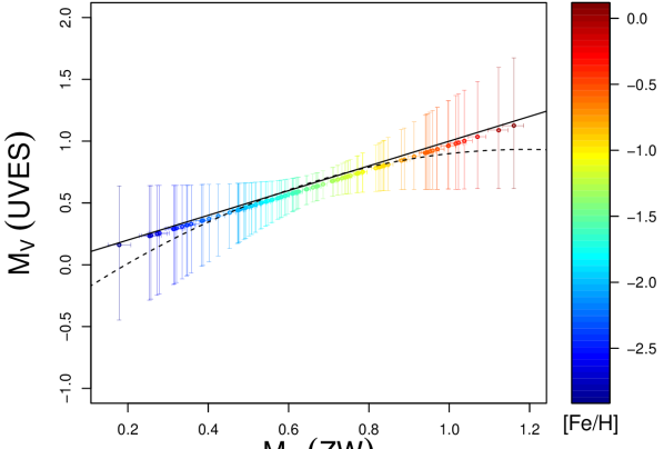
Figure 7: Comparison between $V$-band absolute magnitudes predicted by the linear relationships of Eqs. (13) and (12) when a linear conversion between metallicity scales is applied. The solid and dashed lines represent the bisector and the relation between median magnitudes when a quadratic relation is used to transform between metallicity scales. The colour encodes the metallcity in the ZW scale.

Table 2: Summary statistics associated to the $M_{V}-[\mathrm{Fe/H}]$ relationship by globular cluster RRLs. $M$, $\sigma_{M}$, $\mu_{0}$, ${r}^{\rm{Cl}}$, ${z}^{\rm{RRL}}$ and $\Delta\varpi$ represent the absolute magnitude zero-point, its dispersion, the true distance modulus, the distance to the centre, the RRL median radial projections and the parallax offset inferred by the model for each cluster of our sample, respectively.

GC	RRLs	$M$	$\sigma_{M}$	$\mu_{0}$	${r}^{\rm{Cl}}$	$z^{\rm{RRL}}$	$\Delta\varpi$
		(mag)	(mag)	(mag)	(kpc)	(pc)	(mas)
NGC 3201	59	$0.63_{-0.15}^{+0.13}$	$0.067_{-0.018}^{+0.017}$	$13.45_{-0.13}^{+0.15}$	$4.90_{-0.29}^{+0.36}$	$0.09_{-10.210}^{+9.832}$	$-0.014_{-0.013}^{+0.014}$
NGC 4590	24	$0.39_{-0.38}^{+0.29}$	$0.016_{-0.010}^{+0.015}$	$15.13_{-0.30}^{+0.38}$	$10.63_{-1.35}^{+2.02}$	$0.12_{-0.710}^{+0.472}$	$-0.019_{-0.015}^{+0.016}$
NGC 5824	42	$0.48_{-0.28}^{+0.23}$	$0.083_{-0.009}^{+0.010}$	$17.45_{-0.23}^{+0.28}$	$30.93_{-3.06}^{+4.21}$	$-0.00_{-0.267}^{+0.274}$	$-0.027_{-0.020}^{+0.020}$
NGC 5904	68	$0.64_{-0.15}^{+0.13}$	$0.056_{-0.032}^{+0.030}$	$14.35_{-0.13}^{+0.15}$	$7.41_{-0.42}^{+0.53}$	$2.71_{-70.047}^{+57.861}$	$-0.035_{-0.009}^{+0.009}$
NGC 6121	24	$0.67_{-0.11}^{+0.09}$	$0.097_{-0.017}^{+0.022}$	$11.13_{-0.09}^{+0.11}$	$1.68_{-0.07}^{+0.08}$	$-1.53_{-7.533}^{+12.410}$	$-0.038_{-0.026}^{+0.028}$
NGC 6171	15	$0.72_{-0.19}^{+0.16}$	$0.094_{-0.017}^{+0.024}$	$13.67_{-0.16}^{+0.19}$	$5.43_{-0.40}^{+0.49}$	$-0.06_{-0.450}^{+0.975}$	$-0.041_{-0.016}^{+0.016}$
NGC 6316	2	$0.95_{-0.35}^{+0.36}$	$0.230_{-0.168}^{+0.452}$	$14.24_{-0.42}^{+0.42}$	$7.05_{-1.25}^{+1.50}$	$0.06_{-0.196}^{+0.196}$	$-0.021_{-0.027}^{+0.026}$
NGC 6426	10	$0.35_{-0.47}^{+0.32}$	$0.094_{-0.024}^{+0.032}$	$16.89_{-0.33}^{+0.47}$	$23.86_{-3.36}^{+5.77}$	$-0.03_{-0.080}^{+0.212}$	$-0.032_{-0.022}^{+0.021}$
NGC 6569	11	$0.86_{-0.25}^{+0.31}$	$0.179_{-0.036}^{+0.050}$	$15.42_{-0.33}^{+0.25}$	$12.12_{-1.70}^{+1.51}$	$0.05_{-0.242}^{+0.235}$	$0.011_{-0.022}^{+0.021}$
NGC 6656	22	$0.59_{-0.17}^{+0.16}$	$0.048_{-0.017}^{+0.017}$	$12.69_{-0.16}^{+0.17}$	$3.46_{-0.24}^{+0.27}$	$-0.22_{-5.474}^{+4.922}$	$-0.017_{-0.022}^{+0.021}$
NGC 6864	10	$0.65_{-0.19}^{+0.15}$	$0.126_{-0.026}^{+0.042}$	$16.68_{-0.16}^{+0.19}$	$21.70_{-1.55}^{+2.00}$	$0.09_{-0.221}^{+0.059}$	$-0.033_{-0.023}^{+0.023}$
NGC 7006	43	$0.61_{-0.19}^{+0.15}$	$0.128_{-0.013}^{+0.017}$	$18.00_{-0.15}^{+0.19}$	$39.81_{-2.74}^{+3.65}$	$0.01_{-0.066}^{+0.075}$	$0.001_{-0.021}^{+0.021}$
NGC 7078	27	$0.36_{-0.37}^{+0.30}$	$0.061_{-0.009}^{+0.011}$	$15.17_{-0.30}^{+0.37}$	$10.80_{-1.41}^{+2.02}$	$0.05_{-0.546}^{+0.473}$	$-0.024_{-0.015}^{+0.015}$
Rup 106	8	$0.52_{-0.26}^{+0.20}$	$0.040_{-0.014}^{+0.019}$	$16.83_{-0.21}^{+0.25}$	$23.20_{-2.11}^{+2.89}$	$0.02_{-0.235}^{+0.257}$	$-0.036_{-0.022}^{+0.022}$
Ter 8	1	$0.45_{-0.36}^{+0.26}$	$0.633_{-0.450}^{+0.894}$	$17.13_{-0.62}^{+0.89}$	$26.66_{-6.62}^{+13.51}$	$0.07_{-0.000}^{+0.000}$	$-0.028_{-0.029}^{+0.027}$

Table 3: Upper portion: Summary statistics of the population-level RRL parameters inferred by the $M_{V}-[\mathrm{Fe/H}]$ HM. $\gamma_{1}$, $\gamma_{0}$ and $\tau$ represent the slope, the intercept and the dispersion of the the linear relationship between the mean globular cluster RRL absolute magnitude $\beta_{0}$ and $[\rm{Fe/H}]$ according to Eq. (8), respectively. $\Delta\varpi_{0}$ denotes the parallax zero-point offset calculated as described in the text. Lower Portion: Population-level parameters inferred by the $M_{V}-[\mathrm{Fe/H}]$ HM from our field RRL sample. $\gamma_{1}$, $\gamma_{0}$ and $\tau$ represent the $[\rm{Fe/H}]$ slope, the intercept and the intrinsic dispersion in Eq. (6) of Muraveva et al. (2018), respectively. $\Delta\varpi_{0}$ denotes the parallax zero-point offset calculated as described in the text.

. RRLs sample $\gamma_{1}$ $\gamma_{0}$ $\tau$ ${\Delta\varpi}_{0}$ (mag/dex) (mag) (mag) (mas) GC $0.29_{-0.29}^{+0.35}$ $1.05_{-0.46}^{+0.43}$ $0.108_{-0.080}^{+0.154}$ $-0.024_{-0.008}^{+0.008}$ Field $0.33_{-0.02}^{+0.02}$ $1.13_{-0.03}^{+0.02}$ $0.023_{-0.010}^{+0.012}$ $-0.033_{-0.002}^{+0.002}$

4.3 $M_{G}-{\rm[Fe/H]}$ relation

The GC-level parameters associated to the $M_{G}-{\rm[Fe/H]}$ relation inferred by our HM from the selection of 227 cluster RRLs in the $G$-band are summarised in Table 4, which includes the same parameters as Table 2. The GC mean absolute magnitudes ${M_{G}}_{j}$ (parameter ${\beta_{0j}}$ of Eq. 7) are systematically brighter than the ${M_{V}}_{j}$ magnitudes of Table 2, as expected given the larger passband of the $G$ compared to the $V$ filter. From the cluster-level parallax offsets reported in the rightmost column of the table we infer for the $G$-band data a global parallax offset of ${-0.028_{-0.008}^{+0.009}}$ mas (last column of upper portion of Table 5). The inferred metallicity slope, zero-point and intrinsic dispersion of our GC RRL $M_{G}-{\rm[Fe/H]}$ relation for metal abundances on the Carretta et al. (2009) scale are summarised in the upper portion of Table  5 which translates into the following relationship

$${M_{G}=\left(0.28_{-0.36}^{+0.36}\right)\left[\mathrm{Fe/H}\right]+\left(0.97_{-0.52}^{+0.49}\right)\,,}$$ (18)

with an associated intrinsic dispersion ${\sigma_{M}=0.13_{-0.10}^{+0.18}}$ mag.

We have also updated our previous study of the $M_{G}-{\rm[Fe/H]}$ relation for field RRLs in Muraveva et al. (2018) using the Gaia  EDR3 parallaxes. We present the new results, corresponding to our selection of 223 field RRLs, in the lower portion of Table 5 and Fig. 9. The credible intervals obtained for the metallicity slope and the intercept are $\gamma_{1}^{\rm ZW}=0.33_{-0.02}^{+0.02}$ mag/dex and $\gamma_{0}^{\rm ZW}=1.05_{-0.03}^{+0.03}$ mag, respectively, with an associated intrinsic dispersion of $\sigma_{M}=0.03_{-0.01}^{+0.01}$ mag. Our new inferred $M_{G}-{\rm[Fe/H]}$ relation for field stars with metal abundances on the Zinn & West (1984) metallicity scale is then given by

$$M_{G}=\left(0.33_{-0.02}^{+0.02}\right)\left[\mathrm{Fe/H}\right]+\left(1.05_{-0.03}^{+0.03}\right)\,.$$ (19)

For the $M_{G}-{\rm[Fe/H]}$ relation for field stars we obtained a parallax zero-point offset ${\Delta\varpi}_{0}=-0.033_{-0.002}^{+0.002}$ mas (Table  5, lower portion, last column) calculated using the same procedure used in the previous section.

To compare the relation of Eq. (19) with the GC RRL relation of Eq. (18) we applied the metallicity conversions in Eqs. (15) and (16) to its slope and intercept, and obtained ${\gamma_{1}^{\rm{ZW(UVES)}}=0.31_{-0.40}^{+0.40}}$ mag/dex and ${\gamma_{0}^{\rm{ZW(UVES)}}=1.02_{-0.52}^{+0.49}}$ mag. Using the bootstrapping method we obtained this time a 99 per cent level confidence ellipse for $\boldsymbol{\gamma}^{\mathrm{diff}}$ centred at (0.027 mag/dex, 0.040 mag) with associated MD from its centre equal to 3.03 units. The distance from the coordinate origin (0,0) to the centre of the confidence ellipse was equal to 6.084 units in this case. This latter MD is shorter than the value of 7.94 units reported in Section 4.2 but enough to conclude that the medians $\boldsymbol{\gamma}^{\mathrm{ZW}}$ and $\boldsymbol{\gamma}^{\mathrm{ZW(UVES)}}$ of both pairs of coefficients are significantly different. With regard to the ability of both models to predict consistent absolute magnitudes our results are similar to those reported in the previous section.

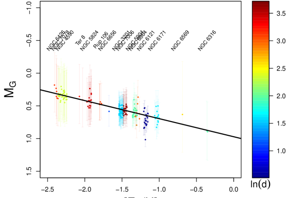
Figure 8: $M_{G}-{\rm[Fe/H]}$ relation defined by globular cluster RRLs as summarized in Table 4. The solid line represents the linear fit corresponding to the parameters of Table 5 (upper portion). The colour scale encodes the (natural) logarithm of the inferred (true) barycentric distance to individual RRL stars measured in units of kpc.

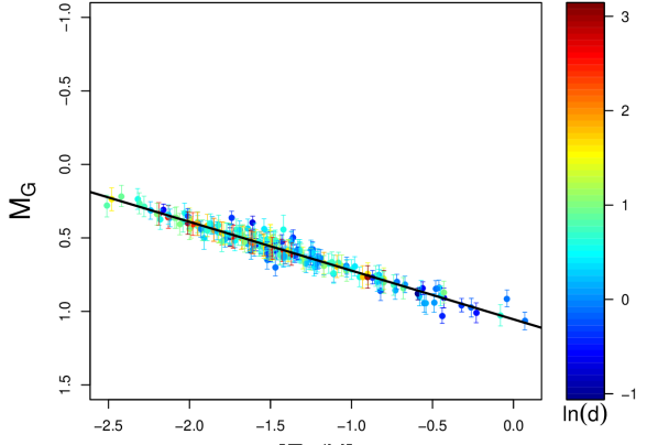
Figure 9: $M_{G}-{\rm[Fe/H]}$ relation defined by our field RRL sample. The solid line represents the linear fit corresponding to the parameters of Table 5 (lower portion). The colour scale encodes the (natural) logarithm of the inferred (true) barycentric distance to individual RRL stars measured in units of kpc.

Table 4: Summary statistics associated to the the $M_{G}-[\mathrm{Fe/H}]$ relationship by globular cluster RRLs. The inferred parameters of each cluster are named as in Table 2.

GC	RRLs	$M$	$\sigma_{M}$	$\mu_{0}$	${r}^{\rm{Cl}}$	$z^{\rm{RRL}}$	$\Delta\varpi$
		(mag)	(mag)	(mag)	(kpc)	(pc)	(mas)
NGC 3201	64	$0.59_{-0.20}^{+0.16}$	$0.063_{-0.008}^{+0.009}$	$13.40_{-0.16}^{+0.20}$	$4.80_{-0.34}^{+0.46}$	$0.17_{-1.370}^{+0.695}$	$-0.021_{-0.016}^{+0.018}$
NGC 4590	21	$0.35_{-0.41}^{+0.37}$	$0.051_{-0.008}^{+0.010}$	$15.10_{-0.37}^{+0.41}$	$10.46_{-1.63}^{+2.17}$	$0.15_{-1.178}^{+0.517}$	$-0.018_{-0.018}^{+0.017}$
NGC 5824	16	$0.43_{-0.36}^{+0.29}$	$0.093_{-0.016}^{+0.023}$	$17.50_{-0.29}^{+0.36}$	$31.58_{-3.90}^{+5.74}$	$0.02_{-0.156}^{+0.218}$	$-0.034_{-0.024}^{+0.025}$
NGC 5904	27	$0.60_{-0.23}^{+0.16}$	$0.072_{-0.022}^{+0.016}$	$14.28_{-0.16}^{+0.23}$	$7.16_{-0.50}^{+0.81}$	$0.40_{-2.735}^{+1.668}$	$-0.041_{-0.012}^{+0.015}$
NGC 6121	21	$0.72_{-0.11}^{+0.11}$	$0.125_{-0.019}^{+0.026}$	$11.20_{-0.10}^{+0.11}$	$1.74_{-0.08}^{+0.09}$	$-0.06_{-1.241}^{+1.454}$	$-0.019_{-0.028}^{+0.028}$
NGC 6171	15	$0.67_{-0.23}^{+0.18}$	$0.099_{-0.018}^{+0.024}$	$13.65_{-0.18}^{+0.23}$	$5.36_{-0.42}^{+0.60}$	$0.19_{-0.939}^{+0.599}$	$-0.043_{-0.017}^{+0.019}$
NGC 6316	2	$0.88_{-0.41}^{+0.38}$	$0.166_{-0.126}^{+0.396}$	$14.26_{-0.43}^{+0.47}$	$7.13_{-1.29}^{+1.71}$	$-0.03_{-0.027}^{+0.027}$	$-0.022_{-0.027}^{+0.027}$
NGC 6426	6	$0.30_{-0.49}^{+0.41}$	$0.108_{-0.034}^{+0.058}$	$16.77_{-0.42}^{+0.49}$	$22.63_{-3.95}^{+5.78}$	$0.07_{-0.245}^{+0.091}$	$-0.031_{-0.024}^{+0.024}$
NGC 6569	1	$0.77_{-0.33}^{+0.28}$	$0.596_{-0.437}^{+0.919}$	$15.64_{-0.58}^{+0.81}$	$13.43_{-3.13}^{+6.10}$	$0.01_{-0.000}^{+0.000}$	$-0.033_{-0.029}^{+0.028}$
NGC 6656	1	$0.53_{-0.25}^{+0.20}$	$0.358_{-0.256}^{+0.640}$	$12.52_{-0.23}^{+0.25}$	$3.18_{-0.33}^{+0.38}$	$-0.00_{-0.000}^{+0.000}$	$-0.025_{-0.028}^{+0.028}$
NGC 6864	8	$0.61_{-0.25}^{+0.18}$	$0.152_{-0.036}^{+0.062}$	$16.56_{-0.19}^{+0.26}$	$20.53_{-1.74}^{+2.60}$	$-0.02_{-0.069}^{+0.089}$	$-0.036_{-0.025}^{+0.024}$
NGC 7006	22	$0.57_{-0.26}^{+0.18}$	$0.055_{-0.009}^{+0.011}$	$18.02_{-0.18}^{+0.25}$	$40.19_{-3.28}^{+4.96}$	$-0.02_{-0.076}^{+0.120}$	$-0.009_{-0.024}^{+0.025}$
NGC 7078	15	$0.34_{-0.42}^{+0.38}$	$0.065_{-0.012}^{+0.016}$	$15.18_{-0.38}^{+0.42}$	$10.88_{-1.74}^{+2.33}$	$0.12_{-0.449}^{+0.308}$	$-0.018_{-0.018}^{+0.017}$
Rup 106	6	$0.47_{-0.31}^{+0.24}$	$0.023_{-0.009}^{+0.014}$	$16.78_{-0.24}^{+0.31}$	$22.67_{-2.34}^{+3.51}$	$0.13_{-0.467}^{+0.402}$	$-0.045_{-0.023}^{+0.024}$
Ter 8	2	$0.42_{-0.41}^{+0.32}$	$0.153_{-0.107}^{+0.444}$	$17.09_{-0.41}^{+0.49}$	$26.12_{-4.52}^{+6.65}$	$0.06_{-0.076}^{+0.076}$	$-0.018_{-0.028}^{+0.029}$

Table 5: Upper portion: Summary statistics of the population-level RRL parameters inferred by the $M_{G}-[\mathrm{Fe/H}]$ HM. Lower portion: Population-level parameters inferred by the by the $M_{G}-[\mathrm{Fe/H}]$ HM from our field RRL sample. Each parameter is named as in Table 3.

RRLs sample	$\gamma_{1}$	$\gamma_{0}$	$\tau$	${\Delta\varpi}_{0}$
	(mag/dex)	(mag)	(mag)	(mas)
GC	$0.28_{-0.36}^{+0.36}$	$0.97_{-0.52}^{+0.49}$	$0.131_{-0.095}^{+0.183}$	$-0.028_{-0.008}^{+0.009}$
Field	$0.33_{-0.02}^{+0.02}$	$1.05_{-0.03}^{+0.03}$	$0.029_{-0.014}^{+0.015}$	$-0.033_{-0.002}^{+0.002}$

4.4 PWZ relations

The literature lacks empirical Period-Metallicity-Wesenheit relations for RR Lyrae stars in the Gaia bands. In this section we use the samples of field and GC RRLs with Gaia EDR3 parallaxes described in Sections 2.1 and 2.2, to calculate a Wesenheit magnitude when intensity-averaged mean magnitudes in the $G$, $G_{\rm BP}$ and $G_{\rm RP}$ bands are simultaneously available for these RRL selections in the Gaia DR2 vari_rrlyrae table. This was possible for 191 field and 168 GC RRLs. To calculate the Wesenheit magnitude we followed the formulation by Ripepi et al. (2019)

$$W\left(G,G_{\rm{BP}},G_{\rm{RP}}\right)=G-\lambda\left(G_{\rm{BP}}-G_{\rm{RP}}\right)\,,$$ (20)

where $\lambda=\frac{A\left(G\right)}{E\left(G_{\rm{BP}}-G_{\rm{RP}}\right)}$. The $\lambda$ value is known to be $\simeq$2 over a wide range of effective temperatures (Andrae et al., 2018). Recently, Ripepi et al. (2019) and Wang & Chen (2019) with independent methods and different stellar samples (Cepheids and Red Clump stars, respectively) obtained $\lambda\simeq 1.90$. To infer a $\lambda$ value appropriate for RRLs we considered table 13 from Jordi et al. (2010) where $\lambda$ estimates are obtained as a combination of effective temperature ($T_{eff}$), gravity (logg) and metallicity. We assumed typical values for RRLs ($T_{eff}$ from 5500 to 7000K; logg from 2.5 to 3) obtaining an average $\lambda$ value of $1.922\pm 0.045$. Since $\lambda$ estimates from Jordi et al. (2010) are based on the average galactic value of $R_{V}=$ 3.1 we adopt the value of $1.922\pm 0.045$ to infer the $PW$ relation for field RRLs sample and for GC RRLs with the exception for the bulge GCs. Indeed we used $\lambda=1.960$ to determine the Wesenheit magnitudes of RRLs members of NGC 6171, NGC 6316, NGC 6656 and NGC 6569 while we adopted $\lambda=2.104$ for RRLs in NGC 6121. Finally, the uncertainties on the Wesenheit magnitudes were computed using the linear error propagation method.

Our selection of 168 cluster RRLs includes only one source belonging to Ter 8, making it impossible to apply our HM to infer a $PW$ relation for this GC. We also removed 15 sources with $G_{\rm BP}$ and $G_{\rm RP}$ photometry available but not reliable. For the remaining 153 RRLs with $W_{(G,G_{\rm BP},G_{\rm RP})}$ magnitudes available, Table 6 summarises the parameters inferred by our HM at GC level. Similarly to the information presented in Tables 2 and 4 for the $V$ and $G$ bands, now the third to the fifth columns provide the period slope ${\beta_{1}}_{j}$, the zero-point ${\beta_{0}}_{j}$ and the intrinsic dispersion ${\sigma_{M}}_{j}$ of the $PW_{(G,G_{\rm BP},G_{\rm RP})}$ relation inferred for each GC according to Eq. (5), and column six gives the average of the GC individual-star mean absolute magnitudes. As in Table 2 we also report the distance modulus of each GC (column 7) and the cluster-level parallax offsets (rightmost column) from which a population-level median parallax offset ${\Delta_{\varpi_{0}}=-0.026_{-0.010}^{+0.010}}$ mas is inferred. Table 6 also summarises, for each GC, the inferred barycentric distance to its centre ($r_{j}^{\rm Cl}$) and the median of the radial distances from the centre to each RRL projected onto the line of sight (${z_{\cdot j}}$).

We do not report the coefficients inferred by our HM at population-level, because they are not reliable values for the slopes and intercept of a $PWZ$ relation that would be incorrectly derived from a sample of RRLs belonging to different absorption environment. Nevertheless, the use of the appropriate ratio of total-to-selective absorption $\lambda$ for each GC in our sample guarantees that the Wesenheit magnitudes in Eq. (20) are correctly defined in the sense that they can be expressed, alternatively, both as a function of the observed or the intrinsic colour (reddening-free property). Hence, the $PW$ relations in Table 6 are correctly derived, and we still can use a subset of them for validation purposes, provided that the $\lambda$ associated with the $PW$ relations in the subset is the same than the $\lambda$ used to derive the Wesenheit magnitudes in the validation dataset (see Section 5).

We now focus on the sample of 191 field RRL stars for which $W_{(G,G_{\rm BP},G_{\rm RP})}$ apparent magnitudes are available. After dropping one source (star SW Her) from the analysis for being largely discrepant with the inferred Period-Wesenheit diagram, we applied the varying parallax offset HM for field stars described in Section 3 to the remaining sample of 190 RRL, thus obtaining the results summarised in Table 7. The inferred $PW_{(G,G_{\rm BP},G_{\rm RP})}Z$ relation is given by

$$\begin{split}W_{\left(G,G_{\rm{BP}},G_{\rm{RP}}\right)}=&\left(-2.49_{-0.20}^{+0.21}\right)\log\left(P\right)+\\ &\left(0.14_{-0.03}^{+0.03}\right)\left[\mathrm{Fe/H}\right]+\left(-0.88_{-0.09}^{+0.08}\right)\,,\\ \end{split}$$ (21)

with an intrinsic dispersion of $0.09\pm{0.01}$ mag and an inferred global parallax offset $\Delta\varpi_{0}=-0.033\pm{0.028}$ mas. The $PW_{(G,G_{\rm BP},G_{\rm RP})}Z$ relation for the 190 field RRLs is shown in Fig. 11. Our inferred parallax zero-point offset associated to this relation is ${\Delta\varpi}_{0}=-0.033_{-0.003}^{+0.003}$ mas (Table 7, lower row).

Eq. (21) is, as far as we know, the first empirical RRL PWZ relation in the Gaia bands calibrated on EDR3 parallaxes.

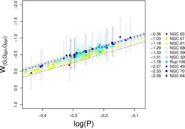
Figure 10: Wesenheit magnitudes inferred by the HM as a function of the decadic logarithm of the true period. The dashed lines represent the $PW_{\left(G,G_{\rm{BP}},G_{\rm{RP}}\right)}$ relations of Eq. (5) particularised for the parameters of Table 6. Colours encode the true metallicity of each globular cluster on the Carretta et al. (2009) metallicity scale according to the scale on the right.

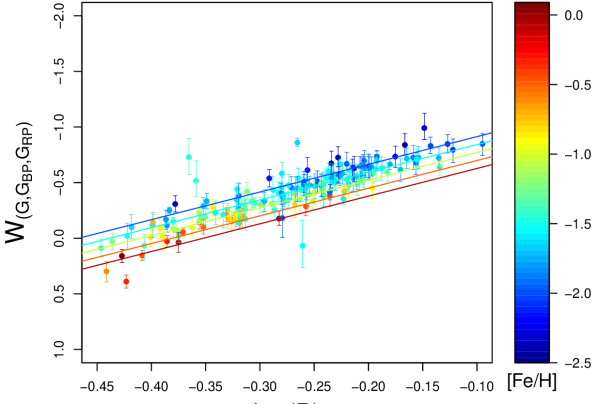
Figure 11: $PW_{\left(G,G_{\rm{BP}},G_{\rm{RP}}\right)}$ distribution of 169 RRLs from our sample of field RRLs, for which absolute $W_{\left(G,G_{\rm{BP}},G_{\rm{RP}}\right)}$ magnitudes were inferred from the model described in Sect. 4 of Muraveva et al. (2018). The lines represent projections of the fit shown by Eq. (21) onto the Magnitude-Period plane. The colour scale encodes values of measured metallicity on the Zinn & West (1984) metallicity scale.

Table 6: Summary statistics of the cluster-level RRL parameters inferred by the $PW_{\left(G,G_{\rm{BP}},G_{\rm{RP}}\right)}Z$ HM. $\beta_{1}$, $\beta_{0}$ and $\sigma_{M}$ represent the $\log(P)$ slope, the zero-point and the intrinsic dispersion of the $j$th cluster $PW_{\left(G,G_{\rm{BP}},G_{\rm{RP}}\right)}$ relationship, and $M$, $\mu_{0}$, ${r}^{\rm{Cl}}$, ${z}^{\rm{RRL}}$ and $\Delta\varpi$ denote the median magnitude of its individual RRL stars, the GC true distance modulus, the distance to the centre, the RRL median radial projections and the parallax zero-point offset.

GC	RRLs	$\beta_{1}$	$\beta_{0}$	$\sigma_{M}$	$M$	$\mu_{0}$	${r}^{\rm{Cl}}$	$z^{\rm{RRL}}$	$\Delta\varpi$
		(mag/dex)	(mag)	(mag)	(mag)	(mag)	(kpc)	(pc)	(mas)
NGC 3201	63	$-2.63_{-0.13}^{+0.18}$	$-1.22_{-0.22}^{+0.18}$	$0.070_{-0.015}^{+0.015}$	$-0.54_{-0.11}^{+0.11}$	$13.39_{-0.18}^{+0.22}$	$4.76_{-0.39}^{+0.51}$	$1.70_{-14.589}^{+7.825}$	$-0.022_{-0.018}^{+0.020}$
NGC 4590	9	$-2.69_{-0.11}^{+0.11}$	$-1.28_{-0.48}^{+0.37}$	$0.013_{-0.009}^{+0.015}$	$-0.49_{-0.33}^{+0.04}$	$15.10_{-0.36}^{+0.49}$	$10.47_{-1.61}^{+2.65}$	$-0.10_{-0.488}^{+0.277}$	$-0.005_{-0.020}^{+0.019}$
NGC 5904	22	$-2.73_{-0.14}^{+0.12}$	$-1.22_{-0.22}^{+0.17}$	$0.059_{-0.012}^{+0.014}$	$-0.42_{-0.18}^{+0.22}$	$14.34_{-0.17}^{+0.22}$	$7.38_{-0.57}^{+0.79}$	$-0.03_{-0.587}^{+0.435}$	$-0.035_{-0.013}^{+0.014}$
NGC 6121	20	$-2.75_{-0.12}^{+0.11}$	$-1.14_{-0.12}^{+0.12}$	$0.035_{-0.017}^{+0.028}$	$-0.39_{-0.20}^{+0.28}$	$11.21_{-0.11}^{+0.11}$	$1.75_{-0.09}^{+0.09}$	$-0.32_{-1.292}^{+2.368}$	$-0.013_{-0.031}^{+0.029}$
NGC 6171	14	$-2.68_{-0.12}^{+0.13}$	$-1.18_{-0.21}^{+0.20}$	$0.059_{-0.020}^{+0.021}$	$-0.22_{-0.28}^{+0.18}$	$13.66_{-0.20}^{+0.21}$	$5.39_{-0.47}^{+0.55}$	$0.35_{-1.549}^{+0.615}$	$-0.036_{-0.018}^{+0.019}$
NGC 6316	2	$-2.70_{-0.16}^{+0.18}$	$-1.07_{-0.41}^{+0.42}$	$0.201_{-0.134}^{+0.424}$	$-0.07_{-0.08}^{+0.08}$	$14.31_{-0.48}^{+0.46}$	$7.27_{-1.44}^{+1.73}$	$0.10_{-0.190}^{+0.190}$	$-0.019_{-0.028}^{+0.029}$
NGC 6426	5	$-2.71_{-0.16}^{+0.16}$	$-1.32_{-0.56}^{+0.41}$	$0.105_{-0.038}^{+0.073}$	$-0.71_{-0.31}^{+0.23}$	$16.76_{-0.42}^{+0.56}$	$22.46_{-3.96}^{+6.66}$	$-0.02_{-0.125}^{+0.113}$	$-0.020_{-0.026}^{+0.027}$
NGC 6864	2	$-2.70_{-0.16}^{+0.18}$	$-1.21_{-0.26}^{+0.19}$	$0.159_{-0.119}^{+0.473}$	$-0.49_{-0.02}^{+0.02}$	$16.95_{-0.28}^{+0.41}$	$24.55_{-2.97}^{+5.09}$	$-0.05_{-0.066}^{+0.066}$	$-0.045_{-0.030}^{+0.029}$
NGC 7078	10	$-2.80_{-0.23}^{+0.15}$	$-1.32_{-0.50}^{+0.39}$	$0.046_{-0.022}^{+0.029}$	$-0.52_{-0.12}^{+0.23}$	$15.14_{-0.39}^{+0.48}$	$10.68_{-1.74}^{+2.66}$	$-0.24_{-0.427}^{+0.830}$	$-0.018_{-0.020}^{+0.020}$
Rup 106	6	$-2.70_{-0.16}^{+0.17}$	$-1.27_{-0.38}^{+0.26}$	$0.092_{-0.029}^{+0.051}$	$-0.73_{-0.03}^{+0.04}$	$16.72_{-0.27}^{+0.39}$	$22.09_{-2.57}^{+4.36}$	$-0.05_{-0.058}^{+0.160}$	$-0.047_{-0.023}^{+0.024}$

Table 7: Population-level parameters inferred by the $PW_{\left(G,G_{\rm{BP}},G_{\rm{RP}}\right)}Z$ HM from our field RRL sample. $\gamma_{2}$, $\gamma_{1}$ and $\gamma_{0}$ represent the $\log(P)$ and $[\rm{Fe/H}]$ slopes and the intercept in Eq. (6) of Muraveva et al. (2018) and $\tau$ denotes the intrinsic dispersion. $\Delta\varpi_{0}$ denotes the parallax zero-point offset.

$\gamma_{2}$	$\gamma_{1}$	$\gamma_{0}$	$\tau$	${\Delta\varpi}_{0}$
(mag/dex)	(mag/dex)	(mag)	(mag)	(mas)
$-2.49_{-0.20}^{+0.21}$	$0.14_{-0.03}^{+0.03}$	$-0.88_{-0.09}^{+0.08}$	$0.09_{-0.01}^{+0.01}$	$-0.033_{-0.003}^{+0.003}$

4.5 Spatial distribution of our samples

One of the advantages of our Bayesian approach is the ability to infer the posterior probability distribution of any parameter of interest in the HM. In this section we present the results of validating the 3D spatial distributions of our field RRLs and the RRLs of some GCs studied in the paper.

For each RRL in the field sample we derived the individual barycentric distance and located the star position in the Galaxy. The measured coordinates $(\alpha,\delta)$ of our RRL stars were first transformed to Galactic coordinates $(l,b)$. For each RR Lyrae we then derived the posterior distribution of its rectangular coordinates $(x_{i},y_{i},z_{i})$ from its posterior parallax ($\varpi_{i}$) in the Cartesian Galactocentric coordinate system of Jurić et al. (2008) by

$$\begin{split}x_{i}^{n}&=R_{\odot}-d_{i}^{n}\cos\left(l_{i}\right)\cos\left(b_{i}\right)\\ y_{i}^{n}&=-d_{i}^{n}\sin\left(l_{i}\right)\cos\left(b_{i}\right)\\ z_{i}^{n}&=d_{i}^{n}\sin\left(b_{i}\right)\,,\\ \end{split}$$ (22)

where $d_{i}^{n}=1/\varpi_{i}^{n}$ denotes the $n$th posterior distance realisation calculated as the reciprocal of the $n$th MCMC posterior parallax realisation, and $R_{\odot}=8.178$ kpc is the adopted distance to the Galactic centre (Gravity Collaboration et al., 2019). The posterior distribution of the radial distance of each star to the Galactic centre were calculated as

$${r_{\mathrm{Gal.Cen.}}}_{i}^{n}=\sqrt{\left(x_{i}^{n}\right)^{2}+\left(y_{i}^{n}\right)^{2}}\,.$$ (23)

Figure 12 represents the spatial distribution and metal abundance of our field RR Lyrae sample in the plane $z-r_{\mathrm{Gal.Cen.}}$ associated with the Galactocentric reference frame.

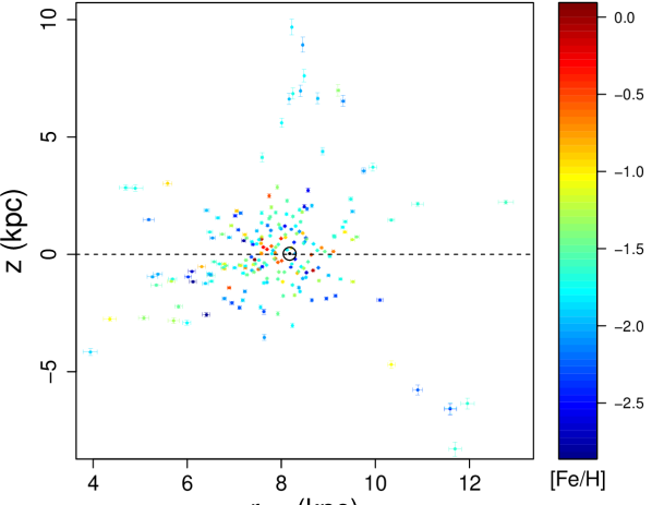
Figure 12: Spatial distribution and metallicity of the field RR Lyrae sample represented in a Galactocentric reference frame. $r_{\rm Gal.Cen.}$ and $z$ denote the radial distance to the Galactic centre and the vertical distance with regard to the Galactic midplane $x-y$, respectively. The Cartesian Galactocentric coordinates and the radial distances to the Galactic centre have been summarised by the median plus/minus the difference in absolute value between the median and the 84th and 16th percentile of the posterior samples of Eqs. (22) and (23).

Aiming to conduct the validation analysis of the 3D spatial distribution for some of the GCs in our sample, we found that, for a fixed GC, the median distances inferred to its centre by our three hierarchical models, which are all consistent within 1$\sigma$, differ by quantities ranging from the order of several tens of pc (NGC 6121 and NGC 5904) to a few kpc (NGC 5824) (see Table 8 in Section 5.1 below). Our most consistent results correspond to NGC 6121, for which the median barycentric distances to its centre inferred by our $M_{G}-{\rm[Fe/H]}$ and $PW_{\left(G,G_{\rm BP},G_{\rm RP}\right)}Z$ hierarchical models are in excellent agreement differing by $\approx$ 10 pc. In what follows we present the results corresponding to the application of our HM for the inference of the $PW_{\left(G,G_{\rm BP},G_{\rm RP}\right)}Z$ relation to the analysis of NGC 6121 spatial distribution. From the measured coordinates $(\alpha_{i},\delta_{i})$ of the $i$th RR Lyrae star belonging to NGC 6121 and the barycentric distance MCMC posterior samples $r_{i}^{n}$ we first derived samples $(x_{i}^{n},y_{i}^{n},z_{i}^{n})$ of the posterior distribution of its rectangular coordinates. Then, based on Weinberg & Nikolaev (2001) we defined, from the spherical coordinates $(\alpha^{\rm Cl},\delta^{\rm Cl})$ of the NGC 6121 centre, a barycentric Cartesian reference frame with the x-axis antiparallel to the $\alpha^{\rm Cl}$ axis, the y-axis parallel to the $\delta^{\rm Cl}$ axis and the z-axis pointing toward the observer, and transformed the samples $(x_{i}^{n},y_{i}^{n},z_{i}^{n})$ to the new frame. We note that the z coordinates in this system are given, from Eq. (10), by $r_{j}^{\mathrm{Cl}}+z_{ij}$ where $z_{ij}$ is the projection of the radial distance from the $i$th source to the cluster centre onto the line of sight. Figure 13 represents the NGC 6121 3D spatial distribution inferred by our $PW_{\left(G,G_{\rm{BP}},G_{\rm{RP}}\right)}Z$ HM projected onto the coordinate planes of the reference frame described above. The three panels of the figure are in the same scale which covers an area of 1600 ${\rm pc}^{2}$. While the marginal RRL distribution associated with the plane of the sky XY is consistent with the $(\alpha,\delta)$ distribution in the middle-right panel of Fig. 2, for the other two planes XZ and YZ we notice that the distribution is elongated along the line of sight (z axis). This non-physical artifact is more prominent for the RRLs closer to the cluster centre as apparent from the angular distances encoded by the colour of the figure.

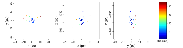
Figure 13: Spatial distribution inferred by our $PW_{\left(G,G_{\rm BP},G_{\rm RP}\right)}Z$ HM for 20 RRLs in NGC 6121 projected onto the coordinate planes associated to the reference frame described in the text. The colour scale encodes the angular separation between the RRLs and the cluster centre. Posterior credible intervals are omitted for clarity, but along the z-axis (line of sight) are on the order of $100$ pc.

5 Validation

5.1 GC distances

In column 6 of Tables 2, 4 and column 8 of Table 6 we reported the credible interval for the distance to the centre of each GC in our sample, inferred by our HM applied to the inference of the $M_{V}-{\rm[Fe/H]}$, $M_{G}-{\rm[Fe/H]}$ and $PW_{\left(G,G_{\rm{BP}},G_{\rm{RP}}\right)}Z$ relations. In this section we compare our three distance estimates with the prior values taken from Harris (1996) (2010 edition, hereafter Harris10) and with GC heliocentric distances reported by the recent literature. Distances in Harris (1996) collection are not the most updated results, but, we think they still form valid priors for our model, since the errors associated with these distances make them all compatible with the most recent literature value. Moreover, adopting the distances contained in the Harris catalogue we guarantee that our results are independent from the most recent literature values which are mainly derived from Gaia EDR3 parallaxes.

An exhaustive study of this topic is beyond the scope of the paper and we only include the minimal information for validation purposes of our own results. We have selected the GC catalogues of Baumgardt et al. (2019) (B19; cf. Table 3), Hernitschek et al. (2019) (H19; cf. Table 10) and Valcin et al. (2020) (V20; cf. Appendix E) which report distances to 53, 59 and 68 Galactic globular clusters, respectively.

Table 8 presents the results of our study. Columns 2, 3 and 4 of the table list the credible intervals for the distance to the centre to each GC of our sample inferred by our HM using the $V$, $G$ and $W\left(G,G_{\mathrm{BP}},G_{\mathrm{RP}}\right)$ data and Gaia EDR3 parallaxes, respectively. The GC distances of Harris10 used as priors in our study are given in column 5, while the literature distances of B19, H19 and V20 are presented in the three rightmost columns of the table. Our distances for the 4 clusters closest to us (NGC 6121, 6656, 3201 and 6171) differ from the literature, at most, by 1 kpc. For those four closest clusters our models report the smallest distances in the table. In particular, for NGC 6121 our models infer distances ranging from 1.68 to 1.75 kpc which are in better agreement with the values by Bhardwaj et al. (2020) which finds true distance moduli for this cluster ranging from 11.241 to 11.323 mag (1.77 to 1.84 kpc). We remark, as pointed out by Hendricks et al. (2012) in their section 5.5, the strong dependency of the true distance to NGC 6121 on the reddening law. As we adopted $R_{V}=3.62$ for this cluster, our distance estimates are also more consistent with the distances reported in table 6 by Hendricks et al. (2012) for larger values of $R_{V}$. The distances we inferred for NGC 5904 (from 7.16 to 7.41 kpc) are also in better agreement with the values found for this cluster by Bhardwaj et al. (2020) (true distance moduli ranging from 14.257 to 14.342 mag corresponding to distances between 7.10 and 7.39 kpc). As in the present work, Bhardwaj et al. (2020) distance moduli are calibrated using Gaia EDR3 parallaxes.

Table 8: Comparison between inferred, prior (Harris10) and literature (B19, H19 and V20) distances to the 15 GCs considered in our study.

GC	${V}$ band	${G}$ band	Wesenheit	Harris10	B19	H19	V20
	(kpc)	(kpc)	(kpc)	(kpc)	(kpc)	(kpc)	(kpc)
NGC 3201	$4.90_{-0.29}^{+0.36}$	$4.80_{-0.34}^{+0.46}$	$4.76_{-0.39}^{+0.51}$	$4.9$	$4.47_{-0.18}^{+0.18}$	$-$	$4.91_{-0.08}^{+0.15}$
NGC 4590	$10.63_{-1.35}^{+2.02}$	$10.46_{-1.63}^{+2.17}$	$10.47_{-1.61}^{+2.65}$	$10.3$	$-$	$10.48_{-0.28}^{+0.26}$	$11.22_{-0.25}^{+0.16}$
NGC 5824	$30.93_{-3.06}^{+4.21}$	$31.58_{-3.90}^{+5.74}$	$-$	$32.1$	$-$	$-$	$-$
NGC 5904	$7.41_{-0.42}^{+0.53}$	$7.16_{-0.50}^{+0.81}$	$7.38_{-0.57}^{+0.79}$	$7.5$	$7.58_{-0.14}^{+0.14}$	$7.87_{-0.19}^{+0.19}$	$7.53_{-0.17}^{+0.11}$
NGC 6121	$1.68_{-0.07}^{+0.08}$	$1.74_{-0.08}^{+0.09}$	$1.75_{-0.09}^{+0.09}$	$2.2$	$1.96_{-0.04}^{+0.04}$	$-$	$2.05_{-0.05}^{+0.03}$
NGC 6171	$5.43_{-0.40}^{+0.49}$	$5.36_{-0.42}^{+0.60}$	$5.39_{-0.47}^{+0.55}$	$6.4$	$5.92_{-0.38}^{+0.38}$	$6.01$	$-$
NGC 6316	$7.05_{-1.25}^{+1.50}$	$7.13_{-1.29}^{+1.71}$	$7.27_{-1.44}^{+1.73}$	$10.4$	$-$	$-$	$-$
NGC 6426	$23.86_{-3.36}^{+5.77}$	$22.63_{-3.95}^{+5.78}$	$22.46_{-3.96}^{+6.66}$	$20.6$	$-$	$19.83$	$21.99_{-1.02}^{+0.85}$
NGC 6569	$12.12_{-1.70}^{+1.51}$	$13.43_{-3.13}^{+6.10}$	$-$	$10.9$	$10.24_{-1.16}^{+1.16}$	$-$	$-$
NGC 6656	$3.46_{-0.24}^{+0.27}$	$3.18_{-0.33}^{+0.38}$	$-$	$3.2$	$3.24_{-0.08}^{+0.08}$	$-$	$3.62_{-0.09}^{+0.09}$
NGC 6864	$21.70_{-1.55}^{+2.00}$	$20.53_{-1.74}^{+2.60}$	$24.55_{-2.97}^{+5.09}$	$20.9$	$-$	$20.79_{-0.35}^{+0.32}$	$-$
NGC 7006	$39.81_{-2.74}^{+3.65}$	$40.19_{-3.28}^{+4.96}$	$-$	$41.2$	$-$	$40.12_{-0.15}^{+0.16}$	$39.78_{-1.41}^{+2.11}$
NGC 7078	$10.80_{-1.41}^{+2.02}$	$10.88_{-1.74}^{+2.33}$	$10.68_{-1.74}^{+2.66}$	$10.4$	$10.21_{-0.13}^{+0.13}$	$11.07_{-0.35}^{+0.32}$	$11.25_{-0.33}^{+0.22}$
Rup 106	$23.20_{-2.11}^{+2.89}$	$22.67_{-2.34}^{+3.51}$	$22.09_{-2.57}^{+4.36}$	$21.2$	$-$	$-$	$21.95_{-0.73}^{+0.73}$
Ter 8	$26.66_{-6.62}^{+13.51}$	$26.12_{-4.52}^{+6.65}$	$-$	$26.3$	$-$	$-$	$28.74_{-0.79}^{+0.99}$

5.2 Distance to the LMC

Table 9: Distance moduli of the LMC obtained from the relations for globular cluster and field RRLs derived in this work.

Relation	Form∗	$\mu_{\rm LMC}$
	Globular Cluster RRLs sample
$M_{V}-{\rm[Fe/H]}$	$M_{V}=\left(0.29_{-0.29}^{+0.35}\right)\left[\mathrm{Fe/H}\right]+\left(1.05_{-0.46}^{+0.43}\right)$	$18.507_{-0.16}^{+0.18}$
$M_{G}-{\rm[Fe/H]}$	$M_{G}=\left(0.28_{-0.36}^{+0.36}\right)\left[\mathrm{Fe/H}\right]+\left(0.97_{-0.52}^{+0.49}\right)$	$18.483_{-0.20}^{+0.26}$
$PW_{(G,G_{\rm BP},G_{\rm RP})}^{\rm{NGC~{}6864}}$	$W=\left(-2.70_{-0.16}^{+0.18}\right)\log\left(P\right)+\left(-1.21_{-0.26}^{+0.19}\right)$	$18.512_{-0.24}^{+0.29}$
$PW_{(G,G_{\rm BP},G_{\rm RP})}^{\rm{NGC~{}5904}}$	$W=\left(-2.73_{-0.14}^{+0.12}\right)\log\left(P\right)+\left(-1.22_{-0.22}^{+0.17}\right)$	$18.503_{-0.19}^{+0.24}$
$PW_{(G,G_{\rm BP},G_{\rm RP})}^{\rm{NGC~{}3201}}$	$W=\left(-2.63_{-0.13}^{+0.18}\right)\log\left(P\right)+\left(-1.22_{-0.22}^{+0.18}\right)$	$18.534_{-0.20}^{+0.23}$
	Field RRLs sample
$M_{V}-{\rm[Fe/H]}$	$M_{V}=\left(0.33_{-0.02}^{+0.02}\right)\left[\mathrm{Fe/H}\right]+\left(1.13_{-0.03}^{+0.02}\right)$	$18.486_{-0.032}^{+0.031}$
$M_{G}-{\rm[Fe/H]}$	$M_{G}=\left(0.33_{-0.43}^{+0.48}\right)\left[\mathrm{Fe/H}\right]+\left(1.05_{-0.03}^{+0.03}\right)$	$18.509_{-0.023}^{+0.022}$
$PW_{(G,G_{\rm BP},G_{\rm RP})}Z$	$W=\left(-2.49_{-0.20}^{+0.21}\right)\log\left(P\right)+\left(0.14_{-0.03}^{+0.03}\right)\left[\mathrm{Fe/H}\right]+\left(-0.88_{-0.09}^{+0.08}\right)$	$18.489_{-0.10}^{+0.11}$
∗Relations for cluster RRLs are reported in the Carretta et al. (2009) metallicity scale, relations for field RRLs are in the
Zinn & West (1984) metallicity scale.

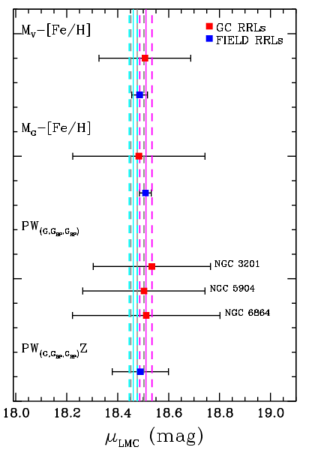
Figure 14: Credible intervals (medians and 16th-84th percentiles) for the distance modulus of the LMC derived according to the procedure described in the text, using the relations for MW field (blue symbols) and GC (red symbols) RRLs inferred in this work. RRL relations and $\mu_{\rm LMC}$ values shown in the figure are listed in columns 2 and 3 of Table 9. We show as references the most accurate and recent LMC distance modulus estimations (solid lines) $\pm 1\sigma$ (dashed lines) by Pietrzyński et al. (2019): $18.477\pm 0.026$ mag (grey) and by Riess et al. (2021b): $18.461\pm 0.016$ (cyan) and $18.511\pm 0.024$ (magenta).

In Sections 4.2 and 4.3 we compared the distributions associated to the median coefficients of two pairs of RRLs relations ($M_{V}-{\rm[Fe/H]}$ and $M_{G}-{\rm[Fe/H]}$) derived in this paper and analysed the consistency between the absolute magnitudes predicted by each pair. In Sect. 4.4, we presented the results corresponding to the $PW_{\left(G,G_{\rm{BP}},G_{\rm{RP}}\right)}Z$ relation for field stars and a set of $PW_{\left(G,G_{\rm{BP}},G_{\rm{RP}}\right)}$ relations for GC stars inferred by our HM and explained why we could not derive a reliable $PWZ$ relation from them. In this section we compare the distances provided by our relations to a universally recognised anchor of the cosmic distance ladder, the Large Magellanic Cloud (LMC). The LMC distance is known with high-accuracy (1$\%$) from eclipsing binary stars (Pietrzyński et al. 2019), hence provides the best place to test and validate the RRL relations we have obtained in this paper. In order to estimate the distance to the LMC we applied the RRL relations inferred in this paper to a sample of 62 stars selected from the catalogue of 70 RRLs located close to the LMC bar described in Muraveva et al. (2015); Muraveva et al. (2018). Spectroscopically measured metallicities are available for these 62 LMC RRLs from the work of Gratton et al. (2004), photometry and absorptions in the $V$-band from Clementini et al. (2003) and pulsation characteristics (periods) from the OGLE-IV catalogue (Soszyński et al., 2019). Since the metallicities of our GC RRL sample are in the Carretta et al. (2009) scale we first converted the metallicities of the 62 LMC RRLs to the Zinn & West (1984) scale by subtracting 0.06 dex (Gratton et al., 2004) and then applied the quadratic relation of Eq. 3 in Carretta et al. (2009) to convert them from the Zinn & West (1984) to the Carretta et al. (2009) metallicity scale. We then crossmatched these 62 RRLs with the Gaia DR2 vari_rrlyrae table and recovered 40 RRLs for which intensity-averaged $G$ mean magnitudes are available and 2 RRLs which also have the corresponding $G_{\mathrm{BP}}$ and $G_{\mathrm{RP}}$ magnitudes. For the 40 RRLs in the $G$ band we estimated the absorption as ${A}_{G}=0.840{A}_{V}$. For the 2 RRLs for which the $G_{\mathrm{BP}}$ and $G_{\mathrm{RP}}$ magnitudes are available we computed the Wesenheit magnitude $W\left(G,G_{\mathrm{BP}},G_{\mathrm{RP}}\right)$ using Eq. (20) and adopting $\lambda=1.922$.

The pairs $\left(\log P,\left[\mathrm{Fe/H}\right]_{\mathrm{UVES}}\right)$ corresponding to these two RRL for which the Wesenheit magnitude are available are equal to $\left(-0.228,-1.47\right)$ and $\left(-0.237,-1.35\right)$, respectively. Since our entire (and representative) sample of 62 RRLs has a median value of the log-period equal to $-0.249$, in order to alleviate a biased estimate of the distance to the LMC, we have selected only the source with its $\log P$ closest to that median value, namely the one having $\log P=-0.237$.

The LMC distance modulus was estimated by Monte Carlo simulations as follows. First, for each (dereddened) apparent magnitude, logarithm of period and metallicity in the three LMC RRL samples described above we generated 10000 realizations of Gaussian distributions with standard deviation equal to the measurement uncertainty. Second, we simulated empirical probability distributions for the individual absolute magnitude $M_{V}$, $M_{G}$ and $W_{\left(G,G_{\rm{BP}},G_{\rm{RP}}\right)}$ in the LMC samples using the MCMC posterior samples of the coefficients and the intrinsic dispersion associated to each fundamental RRL relation inferred by the HM. We generated a univariate distribution for each distance modulus of each RRL and combined these univariate distributions into a joint distribution. Finally, we estimated the LMC distance modulus as the median of the distribution of the medians of each sample of that joint distribution.

The distance moduli of the LMC ($\mu_{\rm LMC}$) predicted by our $M_{V}-{\rm[Fe/H]}$, $M_{G}-{\rm[Fe/H]}$ HMs for GC and field RRLs, the $PW_{(G,G_{\rm BP},G_{\rm RP})}Z$ HM for field RRLs, and a selection of $PW_{(G,G_{\rm BP},G_{\rm RP})}$ relations for GC RRLs are summarised in the rightmost column of Table 9. The selection includes the three GCs with the Wesenheit magnitudes calculated using the same ratio of total-to-selective absorption ($\lambda=1.922$) and having the closest metallicities to the LMC, namely, NGC 6864, NGC 5904 and NGC 3201.
For the $V$-band we report in the first rows of the two portions of the table the credible intervals $\mu_{\rm LMC}^{\rm GC}=18.507_{-0.16}^{+0.18}$ and $\mu_{\rm LMC}^{\rm FS}=18.486_{-0.032}^{+0.031}$, being the difference between their medians of $0.021$ mag. Our predicted LMC distance moduli corresponding to the $G$-band (second rows of the two portions of the table) are $\mu_{\rm LMC}^{\rm GC}=18.483_{-0.20}^{+0.26}$ and $\mu_{\rm LMC}^{\rm FS}=18.509_{-0.14}^{+0.14}$ with a difference between two of $-0.026$ mag. For the $PW_{(G,G_{\rm BP},G_{\rm RP})}$ relations, the inferred LMC distance moduli are $\mu_{\rm LMC}^{\rm NGC~{}3201}=18.534_{-0.20}^{+0.23}$, $\mu_{\rm LMC}^{\rm NGC~{}6864}=18.512_{-0.24}^{+0.29}$, $\mu_{\rm LMC}^{\rm NGC~{}5904}=18.503_{-0.19}^{+0.24}$ while for the $PW_{(G,G_{\rm BP},G_{\rm RP})}(Z)$ relation $\mu_{\rm LMC}^{\rm FS}$ is $18.489_{-0.10}^{+0.11}$ mag. The largest difference of $0.045$ mag between the $\mu_{\rm LMC}$ estimates associated to the $PWZ$ and $PW$ models translates into a difference of $1.04$ kpc in the estimation of the distance to the LMC.

Our eight credible intervals for the LMC distance modulus are plotted in Figure 14. These eight estimates are in good agreement with the value of $\mu_{\rm LMC}$=$18.477\pm 0.026$ mag, reported by Pietrzyński et al. (2019) using a sample of 20 eclipsing binary stars in the LMC and with the two recent estimates by Riess et al. (2021b) of $18.461\pm 0.016$ and $18.511\pm 0.024$ mag derived from their one- and two-parameter solutions using a $PW$ calibration model trained with 75 MW Cepheids and Gaia EDR3 parallaxes. This comparison has the sole purpose of testing the reliability of our relations and how Gaia parallax improvements are reflected in the reassessment of the RRL relations. The errors related to the distance moduli of the LMC are rather large, in particular those obtained with the relations based on the GC RRL sample, compared with the more accurate values present in the literature but also, with those obtained with the relations based on the field RRL sample. The LMC distance inferred from our relations based on the EDR3 parallaxes of the GC RRLs is simply a sanity check, based on data pushed to their limit and it will be superseded by future Gaia releases and more accurate data.

6 Summary and conclusions

Combining a Bayesian hierachical approach with trigonometric parallaxes from the recent Gaia Early Data Release 3, we have derived new RR Lyrae luminosity-metallicity ($M_{V}-{\rm[Fe/H]}$ and $M_{G}-{\rm[Fe/H]}$) relations and the first empirical RRL period-Wesenheit-metallicity relation in the Gaia bands ($PW_{\left(G,G_{\rm{BP}},G_{\rm{RP}}\right)}Z$).

Our analysis is based on two different samples: 291 MW field RRLs and 385 RRLs in 15 Galactic globular clusters spanning metallicity ([Fe/H]) ranges from $-$2.84 to $+$0.07 dex and from $-$2.39 to $-$0.36 dex, respectively. We have used for the RRLs $V$ mean magnitudes, pulsation periods and metal abundances from the literature as well as $G$, $G_{\rm BP}$ and $G_{\rm RP}$ intensity-averaged magnitudes from the Gaia DR2 vari_rrlyrae table (Clementini et al., 2019). Our $M_{V}-{\rm[Fe/H]}$ relation shows a strong dependence of the luminosity on metallicity that is higher than previously found in literature. This relation is however in good agreement with the $M_{V}-{\rm[Fe/H]}$ relation derived by Muraveva et al. (2018) which was calibrated on the Gaia DR2 parallaxes for the same sample of field RRLs.

The Gaia EDR3 parallaxes are still affected by a zero-point offset which, however, is smaller than found for DR2. Lindegren et al. (2020) using quasars (QSOs) estimate that the EDR3 parallaxes are systematically smaller, with a global median offset of $\sim$ $-$0.017 mas and systematic variations at a level of $\sim$ 0.010 mas. Recent analysis of the EDR3 parallaxes, based on independent methods, report different values for the mean parallax zero-point offset: Groenewegen (2021), on a sample of sources with independent trigonometric parallaxes, found a mean offset (EDR3 - independent trigonometric parallaxes) of about $-$0.039 mas, while Bhardwaj et al. (2020) using theoretical PLZ relations for RRLs obtained a small parallax zero-point offset of $-$0.007 $\pm$ 0.003 mas in EDR3 which becomes significantly larger, $-$0.032 $\pm$ 0.004 mas, when the authors apply the corrections proposed by Lindegren et al. (2020). Using our HMs we have obtained independent estimations of the EDR3 parallax offset distribution using the MW field and GC RRLs. We find offset values in the range from $-$0.033 to $-$0.024 mas. These values are in agreement with the results provided both by Lindegren et al. (2020) and Groenewegen (2021).
To test the reliability of our relations we applied them to estimate the distance modulus of the LMC finding values well consistent with the very accurate estimate based on eclipsing binaries by Pietrzyński et al. (2019).

The updated $M_{V}-{\rm[Fe/H]}$ and $M_{G}-{\rm[Fe/H]}$ relations based on field RRLs derived in this paper improve the results reported in table 4 of Muraveva et al. (2018) , being now the intrinsic dispersion of both relations reduced by an order of magnitude.
The relations based on EDR3 parallaxes presented in this paper are expected to further improve with the upcoming full Gaia data release 3 (DR3) in 2022. DR3 will provide, both more accurate time-series photometry of RRLs in the $G$, $G_{\rm BP}$ and $G_{\rm RP}$ bands along with photometric ${\rm[Fe/H]}$ metallicities derived from the light curves as well as astrophysical parameters and, in particular, individual chemical abundances and metal content (${\rm[Fe/H]}$) of the brightest sources (RRLs included) inferred from the $G_{\rm BP}$ and $G_{\rm RP}$ spectra.

Data availability

The data underlying this article are available in the article and in its online supplementary material or will be shared on reasonable request to the corresponding author.

Appendix A RR Lyrae data samples

Table 10: Information on the 291 Galactic field RRLs used in this study. The table is published in its entirety as Supporting Information with the electronic version of the article. A portion is shown here for guidance regarding its form and content.

Name	sourceidEDR3	RAEDR3	DecEDR3	$\varpi_{EDR3}$	$\sigma_{\varpi_{EDR3}}$	Type	P	$V$	$\sigma_{V}$	AV	$\sigma_{A_{V}}$	$G$	$\sigma_{G}$	$G_{BP}$	$\sigma_{G_{BP}}$	$G_{RP}$	$\sigma_{G_{RP}}$	$[Fe/H]$
		(degree)	(degree)	(mas)	(mas)		(days)	(mag)	(mag)	(mag)	(mag)	(mag)	(mag)	(mag)	(mag)	(mag)	(mag)	(dex)
AA Aql	4224859720193721856	$309.562\,793\,571\,088\,2$	$-2.890\,344\,417\,243\,958\,3$	$0.720\,564\,030\,681\,860\,7$	$0.017\,850\,3$	AB	0.3619	$11.822$	$0.012$	$0.27$	$0.043\,200\,001\,716\,613\,77$	$11.815\,822\,236\,294\,224$	$0.0002$	$11.867\,027\,333\,027\,078$	$0.003\,108\,664\,284\,580\,479\,5$	$11.467\,014\,975\,268\,985$	$0.0003$	$-$0.58
AA CMi	3111925220109675136	$109.329\,861\,326\,980\,4$	$1.727\,792\,628\,751\,036\,1$	$0.871\,767\,673\,994\,095$	$0.017\,745\,633$	AB	0.4764	$11.552$	$0.018$	$0.257$	$0.041\,119\,999\,885\,559\,08$	$11.491\,178\,405\,549\,473$	$0.0002$	$11.780\,208\,292\,438\,505$	$0.0004$	$11.025\,686\,468\,473\,275$	$0.0003$	$-$0.55
AA Leo	3915944064285661312	$174.809\,261\,432\,834\,43$	$10.327\,207\,251\,564\,337$	$0.408\,750\,020\,060\,986\,54$	$0.022\,513\,429$	AB	0.5987	$12.332$	$0.012$	$0.115$	$0.018\,400\,000\,333\,786\,012$	$12.219\,307\,300\,493\,71$	$0.0004$	""	""	""	""	$-$1.47
AA Mic	6773950920933073536	$315.173\,189\,792\,987\,56$	$-39.181\,088\,824\,054\,54$	$0.217\,423\,877\,545\,880\,27$	$0.025\,681\,03$	AB	0.4859	$13.943$	$0.019$	$0.114$	$0.018\,240\,000\,009\,536\,742$	$13.842\,517\,117\,731\,603$	$0.0001$	$14.129\,363\,332\,236\,778$	$0.001\,538\,803\,705\,619\,977\,4$	$13.559\,620\,202\,035\,557$	$0.001\,560\,433\,704\,297\,763$	$-$1.17
AB Aps	5779372319228046720	$229.909\,364\,741\,946\,7$	$-78.677\,470\,841\,097\,3$	$0.218\,586\,720\,392\,322\,3$	$0.017\,674\,234$	AB	0.4819	$14.163$	$0.037$	$0.362$	$0.057\,919\,998\,168\,945\,316$	$14.102\,654\,196\,697\,39$	$0.000\,143\,001\,983\,397\,263\,46$	$14.337\,235\,140\,550\,257$	$0.000\,691\,500\,841\,330\,045\,2$	$13.705\,214\,927\,632\,012$	$0.000\,752\,067\,248\,104\,543$	$-$1.30
AB UMa	1546016672688675200	$182.810\,678\,348\,058\,81$	$47.828\,758\,001\,966\,94$	$0.994\,027\,345\,461\,461\,7$	$0.018\,994\,704$	AB	0.5996	$10.899$	$0.018$	$0.068$	$0.010\,880\,000\,591\,278\,076$	$10.787\,574\,892\,292\,092$	$0.000\,083\,721\,188\,856\,104\,75$	$11.052\,949\,861\,665\,663$	$0.000\,073\,690\,571\,076\,854\,4$	$10.395\,166\,404\,923\,85$	$0.000\,108\,777\,074\,209\,114\,01$	$-$0.72
AE Leo	3976785295394882688	$171.550\,865\,657\,693\,6$	$17.660\,902\,377\,168\,89$	$0.370\,573\,260\,590\,598$	$0.018\,770\,542$	AB	0.6268	$12.43$	$0.019$	$0.071$	$0.011\,360\,000\,371\,932\,983$	$12.242\,947\,868\,282\,048$	$0.000\,152\,513\,970\,107\,680\,3$	$12.460\,834\,805\,534\,146$	$0.000\,808\,209\,202\,868\,020\,9$	$11.954\,146\,669\,967\,274$	$0.001\,106\,553\,752\,653\,826$	$-$1.71
AF Vel	5360400630327427072	$163.260\,665\,653\,061\,27$	$-49.906\,384\,603\,983\,6$	$0.830\,806\,573\,799\,542\,3$	$0.015\,529\,353$	AB	0.5275	$11.389$	$0.008$	$0.407$	$0.065\,120\,000\,839\,233\,4$	$11.259\,595\,220\,121\,31$	$0.000\,150\,175\,063\,270\,392\,65$	$11.487\,839\,019\,095\,796$	$0.000\,379\,734\,006\,541\,297\,6$	$10.858\,545\,787\,094\,254$	$0.000\,237\,868\,329\,583\,629\,64$	$-$1.64
AG Tuc	4705269305654137728	$13.722\,443\,824\,474\,775$	$-66.708\,020\,164\,140\,46$	$0.288\,628\,542\,900\,914\,83$	$0.014\,340\,932$	AB	0.6026	$12.861$	$0.036$	$0.046$	$0.007\,360\,000\,014\,305\,115$	$12.778\,369\,312\,644\,912$	$0.000\,204\,097\,000\,942\,130\,33$	$13.088\,480\,709\,104\,484$	$0.000\,714\,983\,114\,740\,17$	$12.462\,201\,271\,307\,35$	$0.000\,499\,390\,586\,892\,767\,5$	$-$1.95
AN Leo	3817504856970457984	$170.843\,673\,313\,886\,9$	$6.634\,628\,638\,755\,927\,5$	$0.448\,252\,364\,029\,558\,8$	$0.016\,654\,43$	AB	0.5721	$12.528$	$0.012$	$0.186$	$0.029\,760\,000\,705\,718\,995$	$12.415\,892\,419\,225\,687$	$0.000\,145\,823\,666\,762\,745\,2$	$12.639\,526\,994\,546\,983$	$0.000\,412\,211\,683\,238\,866\,8$	$11.993\,166\,538\,367\,042$	$0.000\,653\,120\,661\,446\,232\,2$	$-$1.14

Table 11: Sample of 385 RRLs in the Galactic GCs considered in this study. The table is published in its entirety as Supporting Information with the electronic version of the article. A portion is shown here for guidance regarding its form and content.

Cluster	Name	sourceidEDR3	RAEDR3	DecEDR3	$\varpi_{EDR3}$	Type	P	$V$	$G$	$G_{BP}$	$G_{RP}$
		(degree)	(degree)	(mas)		(days)	(mag)	(mag)	(mag)	(mag)
NGC 3201	V1	5413575310452568064	154.4284	$-$46.4438	0.1647$\pm$0.0192	RRAB	0.6048	14.810$\pm$0.006	14.6033$\pm$0.0001	14.9781$\pm$0.0008	14.0203$\pm$0.0005
NGC 3201	V2	5413575520915335936	154.4166	$-$46.4439	0.1840$\pm$0.0224	RRAB	0.5326	14.800$\pm$0.006	14.6296$\pm$0.0002	15.0855$\pm$0.0025	14.1143$\pm$0.0008
NGC 3201	V3	5413575417830877696	154.4769	$-$46.4237	0.2009$\pm$0.0197	RRAB	0.5994	14.910$\pm$0.006	14.6589$\pm$0.0001	15.0761$\pm$0.0009	14.0678$\pm$0.0007
NGC 3201	V4	5413575795793380864	154.4667	$-$46.4112	0.1412$\pm$0.0248	RRAB	0.6300	14.800$\pm$0.006	14.5671$\pm$0.0002	15.0079$\pm$0.0011	14.0107$\pm$0.0007
NGC 3201	V5	5413575555275148672	154.4220	$-$46.4184	0.1942$\pm$0.0251	RRAB	0.5013	14.730$\pm$0.006	14.6018$\pm$0.0002	14.8527$\pm$0.0043	14.0792$\pm$0.0012
NGC 3201	V6	5413574730641610112	154.3587	$-$46.4506	0.1726$\pm$0.0256	RRAB	0.5253	14.740$\pm$0.006	14.5643$\pm$0.0001	14.8966$\pm$0.0013	14.0671$\pm$0.0060
NGC 3201	V7	5413573974727032704	154.3687	$-$46.4635	0.1909$\pm$0.0195	RRAB	0.6303	14.690$\pm$0.006	14.4969$\pm$0.0001	14.8249$\pm$0.0022	13.9259$\pm$0.0028
NGC 3201	V8	5413574077806291456	154.3781	$-$46.4387	0.1272$\pm$0.0253	RRAB	0.6286	14.740$\pm$0.006	14.5398$\pm$0.0001	14.9168$\pm$0.0008	13.9482$\pm$0.0006
NGC 3201	V9	5413574112159737472	154.3845	$-$46.4368	0.1731$\pm$0.0220	RRAB	0.5254	14.820$\pm$0.006	14.6330$\pm$0.0001	15.0181$\pm$0.0010	14.0982$\pm$0.0008
NGC 3201	V10	5413576826585163264	154.3339	$-$46.3472	0.2115$\pm$0.0200	RRAB	0.5352	14.840$\pm$0.006	14.6532$\pm$0.0002	15.0723$\pm$0.0125	14.1087$\pm$0.0006

References

- Alonso-García et al. (2012) Alonso-García J., Mateo M., Sen B., Banerjee M., Catelan M., Minniti D., von Braun K., 2012, AJ, 143, 70
- Andrae et al. (2018) Andrae R., et al., 2018, A&A, 616, A8
- Arellano Ferro et al. (2014) Arellano Ferro A., Ahumada J. A., Calderón J. H., Kains N., 2014, Rev. Mex. Astron. Astrofis., 50, 307
- Arellano Ferro et al. (2016) Arellano Ferro A., Luna A., Bramich D. M., Giridhar S., Ahumada J. A., Muneer S., 2016, Ap&SS, 361, 175
- Barbuy et al. (1998) Barbuy B., Bica E., Ortolani S., 1998, A&A, 333, 117
- Baumgardt et al. (2019) Baumgardt H., Hilker M., Sollima A., Bellini A., 2019, MNRAS, 482, 5138
- Beaton et al. (2016) Beaton R. L., et al., 2016, ApJ, 832, 210
- Bhardwaj et al. (2020) Bhardwaj A., et al., 2020, arXiv e-prints, p. arXiv:2012.13495
- Bica et al. (2016) Bica E., Ortolani S., Barbuy B., 2016, Publ. Astron. Soc. Australia, 33, e028
- Bishop (2013) Bishop C. M., 2013, Philosophical Transactions of the Royal Society Series A, 371, 20120222
- Blažko (1907) Blažko S., 1907, Astronomische Nachrichten, 175, 325
- Bono (2003) Bono G., 2003, in Alloin D., Gieren W., eds, , Stellar Candles for the Extragalactic Distance Scale. Springer Berlin Heidelberg, Berlin, Heidelberg, pp 85–104, doi:10.1007/978-3-540-39882-0_5, https://doi.org/10.1007/978-3-540-39882-0_5
- Bono et al. (2003) Bono G., Caputo F., Castellani V., Marconi M., Storm J., Degl’Innocenti S., 2003, MNRAS, 344, 1097
- Bono et al. (2019) Bono G., et al., 2019, ApJ, 870, 115
- Braga et al. (2015) Braga V. F., et al., 2015, ApJ, 799, 165
- Cacciari & Clementini (2003) Cacciari C., Clementini G., 2003, in Alloin D., Gieren W., eds, , Stellar Candles for the Extragalactic Distance Scale. Springer Berlin Heidelberg, Berlin, Heidelberg, pp 105–122, doi:10.1007/978-3-540-39882-0_6, https://doi.org/10.1007/978-3-540-39882-0_6
- Caputo et al. (2000) Caputo F., Castellani V., Marconi M., Ripepi V., 2000, MNRAS, 316, 819
- Cardelli et al. (1989) Cardelli J. A., Clayton G. C., Mathis J. S., 1989, ApJ, 345, 245
- Carpenter et al. (2017) Carpenter B., et al., 2017, Journal of Statistical Software, 76, 1
- Carretta et al. (2009) Carretta E., Bragaglia A., Gratton R., D’Orazi V., Lucatello S., 2009, A&A, 508, 695
- Catelan et al. (2004) Catelan M., Pritzl B. J., Smith H. A., 2004, ApJS, 154, 633
- Clement & Shelton (1997) Clement C. M., Shelton I., 1997, AJ, 113, 1711
- Clementini et al. (2003) Clementini G., Gratton R., Bragaglia A., Carretta E., Di Fabrizio L., Maio M., 2003, AJ, 125, 1309
- Clementini et al. (2019) Clementini G., et al., 2019, A&A, 622, A60
- Coppola et al. (2011) Coppola G., et al., 2011, MNRAS, 416, 1056
- Corwin et al. (2003) Corwin T. M., Catelan M., Smith H. A., Borissova J., Ferraro F. R., Raburn W. S., 2003, AJ, 125, 2543
- Corwin et al. (2008) Corwin T. M., Borissova J., Stetson P. B., Catelan M., Smith H. A., Kurtev R., Stephens A. W., 2008, AJ, 135, 1459
- Dambis et al. (2013) Dambis A. K., Berdnikov L. N., Kniazev A. Y., Kravtsov V. V., Rastorguev A. S., Sefako R., Vozyakova O. V., 2013, MNRAS, 435, 3206
- Delgado et al. (2019) Delgado H. E., Sarro L. M., Clementini G., Muraveva T., Garofalo A., 2019, A&A, 623, A156
- Di Valentino (2021) Di Valentino E., 2021, MNRAS, 502, 2065
- Dias et al. (2016) Dias B., Barbuy B., Saviane I., Held E. V., Da Costa G. S., Ortolani S., Gullieuszik M., Vásquez S., 2016, A&A, 590, A9
- Dickens (1970) Dickens R. J., 1970, ApJS, 22, 249
- Drake et al. (2013) Drake A. J., et al., 2013, ApJ, 763, 32
- Feeney et al. (2018) Feeney S. M., Mortlock D. J., Dalmasso N., 2018, MNRAS, 476, 3861
- Freedman (2021) Freedman W. L., 2021, arXiv e-prints, p. arXiv:2106.15656
- Gaia Collaboration et al. (2017) Gaia Collaboration et al., 2017, A&A, 605, A79
- Gaia Collaboration et al. (2020) Gaia Collaboration Brown A. G. A., Vallenari A., Prusti T., de Bruijne J. H. J., Babusiaux C., Biermann M., 2020, arXiv e-prints, p. arXiv:2012.01533
- Ghahramani (2015) Ghahramani Z., 2015, Nature, 521, 452
- Gratton et al. (2004) Gratton R. G., Bragaglia A., Clementini G., Carretta E., Di Fabrizio L., Maio M., Taribello E., 2004, A&A, 421, 937
- Gravity Collaboration et al. (2019) Gravity Collaboration et al., 2019, A&A, 625, L10
- Groenewegen (2021) Groenewegen M., 2021, arXiv e-prints, p. arXiv:2106.08128
- Grubissich (1958) Grubissich C., 1958, Contributi dell’Osservatorio Astrofisica dell’Universita di Padova in Asiago, 94, 1
- Hall et al. (2019) Hall O. J., et al., 2019, MNRAS, 486, 3569
- Harris (1996) Harris W. E., 1996, AJ, 112, 1487
- Hawkins et al. (2017) Hawkins K., Leistedt B., Bovy J., Hogg D. W., 2017, MNRAS, 471, 722
- Hazen-Liller (1985) Hazen-Liller M. L., 1985, AJ, 90, 1807
- Hendricks et al. (2012) Hendricks B., Stetson P. B., VandenBerg D. A., Dall’Ora M., 2012, AJ, 144, 25
- Hernitschek et al. (2019) Hernitschek N., et al., 2019, ApJ, 871, 49
- Hoffman & Gelman (2014) Hoffman M. D., Gelman A., 2014, J. Mach. Learn. Res., 15, 1593
- Jordi et al. (2010) Jordi C., et al., 2010, A&A, 523, A48
- Jurić et al. (2008) Jurić M., et al., 2008, ApJ, 673, 864
- Kains et al. (2015) Kains N., et al., 2015, A&A, 578, A128
- Kaluzny et al. (1995) Kaluzny J., Krzeminski W., Mazur B., 1995, AJ, 110, 2206
- Kaluzny et al. (2000) Kaluzny J., Olech A., Thompson I., Pych W., Krzeminski W., Schwarzenberg-Czerny A., 2000, A&AS, 143, 215
- Kaluzny et al. (2013) Kaluzny J., Thompson I. B., Rozyczka M., Krzeminski W., 2013, Acta Astron., 63, 181
- Kunder et al. (2013) Kunder A., et al., 2013, AJ, 146, 119
- Lauritzen (1996) Lauritzen S., 1996, Graphical Models. Oxford University Press
- Layden & Sarajedini (2003) Layden A. C., Sarajedini A., 2003, AJ, 125, 208
- Layden et al. (2003) Layden A. C., Bowes B. T., Welch D. L., Webb T. M. A., 2003, AJ, 126, 255
- Lindegren (2018) Lindegren L., 2018, Technical Note GAIA-C3-TN-LU-LL-124, http://www.rssd.esa.int/doc_fetch.php?id=3757412
- Lindegren et al. (2020) Lindegren L., et al., 2020, arXiv e-prints, p. arXiv:2012.01742
- Longmore et al. (1986) Longmore A. J., Fernley J. A., Jameson R. F., 1986, MNRAS, 220, 279
- Madore (1982) Madore B. F., 1982, ApJ, 253, 575
- Madore et al. (2013) Madore B. F., et al., 2013, ApJ, 776, 135
- Mahalanobis (1936) Mahalanobis P. C., 1936, Proc. Natl. Inst. Sci. India, 2, 49
- Mandel et al. (2009) Mandel K. S., Wood-Vasey W. M., Friedman A. S., Kirshner R. P., 2009, ApJ, 704, 629
- Marconi et al. (2015) Marconi M., et al., 2015, ApJ, 808, 50
- Marconi et al. (2021) Marconi M., Molinaro R., Ripepi V., Leccia S., Musella I., De Somma G., Gatto M., Moretti M. I., 2021, MNRAS, 500, 5009
- Muraveva et al. (2015) Muraveva T., et al., 2015, ApJ, 807, 127
- Muraveva et al. (2018) Muraveva T., Delgado H. E., Clementini G., Sarro L. M., Garofalo A., 2018, MNRAS, 481, 1195
- Neeley et al. (2017) Neeley J. R., et al., 2017, ApJ, 841, 84
- Neeley et al. (2019) Neeley J. R., et al., 2019, MNRAS, 490, 4254
- Ninkovic (1998) Ninkovic S., 1998, Serbian Astronomical Journal, 158
- Oosterhoff (1941) Oosterhoff P. T., 1941, Annalen van de Sterrewacht te Leiden, 17, D1
- Ordoñez & Sarajedini (2016) Ordoñez A. J., Sarajedini A., 2016, MNRAS, 455, 2163
- Papadakis et al. (2000) Papadakis I., Hatzidimitriou D., Croke B. F. W., Papamastorakis I., 2000, AJ, 119, 851
- Pearl (1988) Pearl J., 1988, Probabilistic Reasoning in Intelligent Systems: Networks of Plausble Inference. Morgan Kaufmann Pub
- Pietrzyński et al. (2019) Pietrzyński G., et al., 2019, Nature, 567, 200
- R Core Team (2017) R Core Team 2017, R: A Language and Environment for Statistical Computing. R Foundation for Statistical Computing, Vienna, Austria, https://www.R-project.org/
- Riess et al. (2021a) Riess A. G., et al., 2021a, arXiv e-prints, p. arXiv:2112.04510
- Riess et al. (2021b) Riess A. G., Casertano S., Yuan W., Bowers J. B., Macri L., Zinn J. C., Scolnic D., 2021b, ApJ, 908, L6
- Ripepi et al. (2019) Ripepi V., Molinaro R., Musella I., Marconi M., Leccia S., Eyer L., 2019, A&A, 625, A14
- Salinas et al. (2005) Salinas R., Catelan M., Smith H. A., Pritzl B. J., Borissova J., 2005, Information Bulletin on Variable Stars, 5640, 1
- Samus et al. (2009) Samus N. N., Kazarovets E. V., Pastukhova E. N., Tsvetkova T. M., Durlevich O. V., 2009, PASP, 121, 1378
- Sandage (1993) Sandage A., 1993, AJ, 106, 703
- Schlafly & Finkbeiner (2011) Schlafly E. F., Finkbeiner D. P., 2011, ApJ, 737, 103
- Scott et al. (2006) Scott N. J., Corwin T. M., Catelan M., Smith H. A., 2006, Information Bulletin on Variable Stars, 5706, 1
- Sesar et al. (2017) Sesar B., Fouesneau M., Price-Whelan A. M., Bailer-Jones C. A. L., Gould A., Rix H.-W., 2017, ApJ, 838, 107
- Sollima et al. (2006) Sollima A., Cacciari C., Valenti E., 2006, MNRAS, 372, 1675
- Soszyński et al. (2014) Soszyński I., et al., 2014, Acta Astron., 64, 177
- Soszyński et al. (2019) Soszyński I., et al., 2019, Acta Astron., 69, 87
- Stan Development Team (2018) Stan Development Team 2018, RStan: the R interface to Stan, %****␣main.bbl␣Line␣525␣****http://mc-stan.org/
- Stassun & Torres (2021) Stassun K. G., Torres G., 2021, ApJ, 907, L33
- Stetson et al. (2014) Stetson P. B., et al., 2014, PASP, 126, 521
- Taylor (2005) Taylor M. B., 2005, in Shopbell P., Britton M., Ebert R., eds, Astronomical Society of the Pacific Conference Series Vol. 347, Astronomical Data Analysis Software and Systems XIV. p. 29
- Torrealba et al. (2015) Torrealba G., et al., 2015, MNRAS, 446, 2251
- Valcin et al. (2020) Valcin D., Bernal J. L., Jimenez R., Verde L., Wandelt B. D., 2020, J. Cosmology Astropart. Phys., 2020, 002
- Verde et al. (2019) Verde L., Treu T., Riess A. G., 2019, Nature Astronomy, 3, 891
- Walker et al. (2017) Walker A. R., et al., 2017, AJ, 154, 8
- Wang & Chen (2019) Wang S., Chen X., 2019, ApJ, 877, 116
- Wehlau et al. (1999) Wehlau A., Slawson R. W., Nemec J. M., 1999, AJ, 117, 286
- Weinberg & Nikolaev (2001) Weinberg M. D., Nikolaev S., 2001, ApJ, 548, 712
- Yao et al. (1988) Yao B. A., Tong J. H., Zhang C. S., 1988, Acta Astronomica Sinica, 29, 243
- Zinn (2021) Zinn J. C., 2021, arXiv e-prints, p. arXiv:2101.07252
- Zinn & West (1984) Zinn R., West M. J., 1984, ApJS, 55, 45
- van den Bergh (1975) van den Bergh S., 1975, in Sandage A., Sandage M., Kristian J., eds, , Galaxies and the Universe. University of Chicago, Chicago, IL, p. 509