$\mathcal{H}_{\infty}$-Optimal Interval Observer Synthesis for Uncertain Nonlinear Dynamical Systems via Mixed-Monotone Decompositions

Abstract

This paper introduces a novel $\mathcal{H}_{\infty}$-optimal interval observer synthesis for bounded-error/uncertain locally Lipschitz nonlinear continuous-time (CT) and discrete-time (DT) systems with noisy nonlinear observations. Specifically, using mixed-monotone decompositions, the proposed observer is correct by construction, i.e., the interval estimates readily frame the true states without additional constraints or procedures. In addition, we provide sufficient conditions for input-to-state (ISS) stability of the proposed observer and for minimizing the $\mathcal{H}_{\infty}$ gain of the framer error system in the form of semi-definite programs (SDPs) with Linear Matrix Inequalities (LMIs) constraints. Finally, we compare the performance of the proposed $\mathcal{H}_{\infty}$-optimal interval observers with some benchmark CT and DT interval observers.

I Introduction

Engineering applications, e.g., monitoring, system identification, control synthesis, and fault detection often require knowledge of system states. However, due to the presence of noise/ uncertainties and/or inaccuracies in sensor measurements, system states are usually not exactly known. This has motivated the design of state observers to estimate system states using uncertain/noisy observations and system dynamics. In particular, for bounded-error settings, i.e., when uncertainties are set-valued (and distribution-free), interval observer designs have recently gained much attention due to their simple principles and computational efficiency [1].

Recent years have produced an extensive body of seminal literature on the design of interval/set-valued observers for several classes of systems, e.g., linear, cooperative/monotone, Metzler and mixed-monotone dynamics [1, 2, 3, 4, 5]. It has been noted that the design of interval observers that must simultaneously satisfy correctness (framer property) and stability/convergence is not a trivial task, even for linear systems [2]. Thus, especially when the system dynamics is nonlinear, either relatively restrictive assumptions on system properties were required to guarantee the applicability of the proposed approaches, or monotone systems properties [6] need to be directly imposed to satisfy positivity/cooperative behavior of the error dynamics.

This challenge has been addressed for specific system classes by leveraging Müller’s theorem or interval arithmetic-based approaches [7], transformation to a positive system before designing an observer (only for linear systems) [8] or applying time-invariant/varying state transformations [3]. On the other hand, the work in [9] leveraged bounding functions to design interval observers for a class of continuous-time nonlinear systems under some relatively restrictive assumptions on the nonlinear dynamics, without providing a systematic approach to compute the bounding functions nor necessary/sufficient conditions for their existence. More recently, bounding/mixed-monotone decomposition functions were applied in [3] to design interval observers for nonlinear discrete-time dynamics, where conservative additive terms were added to the error dynamics to guarantee its positivity. Moreover, to best of our understanding, the resulting Linear Matrix Inequalities (LMIs) do not include the required conditions to guarantee that the computed bounding functions are decomposition functions.

Decomposition functions were also applied in the authors’ previous work [4, 5] to design interval observers for nonlinear discrete-time systems under the (restrictive) assumption of global Lipschitz continuity as well as additional sufficient structural system properties to guarantee stability. Further, the applied decomposition functions were not necessarily the tightest. In our preliminary work [10], we proposed an interval observer design for noiseless nonlinear CT and DT systems based on tight remainder-form decomposition functions [11]. Our goal is to extend the design in [10] to noisy uncertain nonlinear dynamics in this work.

In particular, in this paper, we propose a unified framework to synthesize $\mathcal{H}_{\infty}$- optimal and input-to-state stable (ISS) interval observes for a very broad range of locally Lipschitz bounded-error nonlinear CT and DT systems with noisy nonlinear observation functions. Using remainder-form mixed-monotone decomposition functions [11], we show that the states of the designed observer frame the true state trajectory of the system for all possible realizations of interval-valued noise/disturbance and initial states, i.e, the proposed observer is correct-by-construction, without imposing additional constraints or assumptions. Further, we formulate semi-definite programs (SDPs) with LMI constraints for both CT and DT cases to minimize the $\mathcal{H}_{\infty}$-gain of the framer error (interval width) system and to ensure input-to-state stability of the correct-by-construction framers, which can be computed offline to find the stabilizing observer gains.

II Preliminaries

Notation. $\mathbb{R}^{n},\mathbb{R}^{n\times p},\mathbb{D}_{n},\mathbb{N},\mathbb{N}_{n}$ denote the $n$-dimensional Euclidean space and the sets of $n$ by $p$ matrices, $n$ by $n$ diagonal matrices, natural numbers and natural numbers up to $n$, respectively, while $\mathbb{M}_{n}$ denote s the set of all $n$ by $n$ Metzler matrices. For $M\in\mathbb{R}^{n\times p}$, $M_{ij}$ denotes $M$’s entry in the $i$’th row and the $j$’th column, $M^{+}\triangleq\max(M,\mathbf{0}_{n,p})$, $M^{-}=M^{+}-M$ and $|M|\triangleq M^{+}+M^{-}$, where $\mathbf{0}_{n,p}$ is the zero matrix in $\mathbb{R}^{n\times p}$, while $\textstyle{\mathrm{sgn}}(M)\in\mathbb{R}^{n\times p}$ is the element-wise sign of $M$ with $\textstyle{\mathrm{sgn}}(M_{ij})=1$ if $M_{ij}\geq 0$ and $\textstyle{\mathrm{sgn}}(M_{ij})=-1$, otherwise. Further, if $p=n$, $M^{\text{d}}$ denotes a diagonal matrix whose diagonal coincides with the diagonal of $M$, $M^{\text{nd}}\triangleq M-M^{\text{d}}$ and $M^{\text{m}}\triangleq M^{\text{d}}+|M^{\text{nd}}|$, while $M\succ 0$ and $M\prec 0$ (or $M\succeq 0$ and $M\preceq 0$) denote that $M$ is positive and negative (semi-)definite, respectively. Finally, a function $f:S\subseteq\mathbb{R}^{n}\to\mathbb{R}$, where $0\in S$, is positive definite if $f(x)>0$ for all $x\in S{\color[rgb]{0,0,0}\,\setminus\{0\}}$, and $f(0)=0$.

Next, we introduce some useful definitions and results.

Definition 1 (Interval, Maximal and Minimal Elements, Interval Width).

An (multi-dimensional) interval $\mathcal{I}\triangleq[\underline{{\color[rgb]{0,0,0}z}},\overline{{\color[rgb]{0,0,0}z}}]\subset\mathbb{R}^{n}$ is the set of all real vectors ${\color[rgb]{0,0,0}z\in\mathbb{R}^{n_{z}}}$ that satisfies $\underline{{\color[rgb]{0,0,0}z}}\leq{\color[rgb]{0,0,0}z}\leq\overline{{\color[rgb]{0,0,0}z}}$, where $\underline{{\color[rgb]{0,0,0}z}}$, $\overline{{\color[rgb]{0,0,0}z}}$ and $\|\overline{{\color[rgb]{0,0,0}z}}-\underline{{\color[rgb]{0,0,0}z}}\|{\color[rgb]{0,0,0}_{\infty}\triangleq\max_{i\in\{1,\cdots,{\color[rgb]{0,0,0}n_{z}}\}}{\color[rgb]{0,0,0}|z_{i}|}}$ are called minimal vector, maximal vector and interval width of $\mathcal{I}$, respectively. An interval matrix can be defined similarly.

Proposition 1.

[9, Lemma 1] Let $A\in\mathbb{R}^{n\times p}$ and $\underline{x}\leq x\leq\overline{x}\in\mathbb{R}^{n}$. Then , $A^{+}\underline{x}-A^{-}\overline{x}\leq Ax\leq A^{+}\overline{x}-A^{-}\underline{x}$. As a corollary, if $A$ is non-negative, $A\underline{x}\leq Ax\leq A\overline{x}$.

Definition 2 (Jacobian Sign-Stability).

A mapping $f:{\color[rgb]{0,0,0}\mathcal{Z}}\subset\mathbb{R}^{\color[rgb]{0,0,0}n_{z}}\to\mathbb{R}^{p}$ is (generalized) Jacobian sign-stable (JSS), if its (generalized) Jacobian matrix entries do not change signs on its domain, i.e., if either of the following hold:

$$\forall{\color[rgb]{0,0,0}z\in\mathcal{Z}},\forall i\in\mathbb{N}_{p},\forall j\in\mathbb{N}_{n_{z}},J^{f}_{ij}({\color[rgb]{0,0,0}z})\geq 0\ \text{(positive JSS)},$$

$$\forall{\color[rgb]{0,0,0}z\in\mathcal{Z}},\forall i\in\mathbb{N}_{p},\forall j\in\mathbb{N}_{n_{z}},J^{f}_{ij}({\color[rgb]{0,0,0}z})\leq 0\ \text{(negative JSS)},$$

where $J^{f}({\color[rgb]{0,0,0}z})$ denotes the Jacobian matrix of $f$ at ${\color[rgb]{0,0,0}z\in\mathcal{Z}}$.

Proposition 2 (Jacobian Sign-Stable Decomposition, [10, Proposition 2]).

Let $f:{\color[rgb]{0,0,0}\mathcal{Z}}\subset\mathbb{R}^{n_{z}}\to\mathbb{R}^{p}$ and suppose $\forall{\color[rgb]{0,0,0}z\in\mathcal{Z}},J^{f}({\color[rgb]{0,0,0}z})\in[\underline{J}^{f},\overline{J}^{f}]$, where $\underline{J}^{f},\overline{J}^{f}$ are known matrices in $\mathbb{R}^{p\times n_{z}}$. Then, $f$ can be decomposed into a (remainder) affine mapping $H{\color[rgb]{0,0,0}z}$ and a JSS mapping $\mu(\cdot)$, in an additive form:

$$\forall{\color[rgb]{0,0,0}z\in\mathcal{Z}},f({\color[rgb]{0,0,0}z})=\mu({\color[rgb]{0,0,0}z})+H{\color[rgb]{0,0,0}z},$$ (1)

where $H$ is a matrix in $\mathbb{R}^{p\times n_{z}}$, that satisfies the following

$$\forall(i,j)\in\mathbb{N}_{p}\times\mathbb{N}_{n_{z}},H_{ij}=\overline{J}^{f}_{i,j}\ \lor H_{ij}=\underline{J}^{f}_{ij}.$$ (2)

Definition 3 (Mixed-Monotonicity and Decomposition Functions).

[12, Definition 1],[13, Definition 4] Consider the bounded-error dynamical system with initial state $x_{0}\in\mathcal{X}_{0}\triangleq[\underline{x}_{0},\overline{x}_{0}]{\color[rgb]{0,0,0}\subset\mathbb{R}^{n}}$ and process noise $w_{t}\in\mathcal{W}\triangleq[\underline{w},\overline{w}]\subset\mathbb{R}^{n_{w}}$:

$$x_{t}^{+}={\color[rgb]{0,0,0}g(z_{t})\triangleq}g(x_{t},{\color[rgb]{0,0,0}w_{t}}),{\color[rgb]{0,0,0}z_{t}\triangleq[x^{\top}_{t}\ w_{t}]^{\top}}$$ (3)

where $x_{t}^{+}\triangleq x_{t+1}$ if (3) is a DT system and $x_{t}^{+}\triangleq\dot{x}_{t}$ if (3) is a CT system. Moreover, ${g}:{\color[rgb]{0,0,0}\mathcal{Z}}\subset\mathbb{R}^{\color[rgb]{0,0,0}n_{z}}\to\mathbb{R}^{{\color[rgb]{0,0,0}n}}$ is the vector field with augmented state ${\color[rgb]{0,0,0}z_{t}}\in{\color[rgb]{0,0,0}\mathcal{Z}\triangleq\mathcal{X}\times\mathcal{W}\subset\mathbb{R}^{n_{z}}}$ as its domain, where $\mathcal{X}$ is the entire state space and $n_{z}=n+n_{w}$.

Suppose (3) is a DT system. Then, a mapping $g_{d}:{\color[rgb]{0,0,0}\mathcal{Z}\times\mathcal{Z}}\to\mathbb{R}^{p}$ is a DT mixed-monotone decomposition function with respect to $g$, if i) $g_{d}({\color[rgb]{0,0,0}z,z})=g({\color[rgb]{0,0,0}z})$, ii) $g_{d}$ is monotone increasing in its first argument, i.e., $\hat{{\color[rgb]{0,0,0}z}}\geq{\color[rgb]{0,0,0}z}\Rightarrow g_{d}(\hat{{\color[rgb]{0,0,0}z}},{\color[rgb]{0,0,0}z}^{\prime})\geq g_{d}({\color[rgb]{0,0,0}z,z}^{\prime})$, and iii) $g_{d}$ is monotone decreasing in its second argument, i.e., $\hat{{\color[rgb]{0,0,0}z}}\geq{\color[rgb]{0,0,0}z}\Rightarrow g_{d}({\color[rgb]{0,0,0}z}^{\prime},\hat{{\color[rgb]{0,0,0}z}})\leq g_{d}({\color[rgb]{0,0,0}z}^{\prime},{\color[rgb]{0,0,0}z}).$

On the other hand, if (3) is a CT system, a mapping $g_{d}:{\color[rgb]{0,0,0}\mathcal{Z}\times\mathcal{Z}}\to\mathbb{R}^{p}$ is a CT mixed-monotone decomposition function with respect to $g$, if i) $g_{d}({\color[rgb]{0,0,0}z},{\color[rgb]{0,0,0}z})=g({\color[rgb]{0,0,0}z})$, ii) $g_{d}$ is monotone increasing in its first argument with respect to “off-diagonal” arguments, i.e., $\forall(i,j)\in\mathbb{N}_{{\color[rgb]{0,0,0}n}}\times\mathbb{N}_{{\color[rgb]{0,0,0}n_{z}}}\land i\neq j,{\color[rgb]{0,0,0}\hat{z}}_{j}\geq{\color[rgb]{0,0,0}z}_{j},{\color[rgb]{0,0,0}\hat{z}_{i}=z_{i}}\Rightarrow g_{d,i}(\hat{{\color[rgb]{0,0,0}z}},{\color[rgb]{0,0,0}z}^{\prime})\geq g_{d,i}({\color[rgb]{0,0,0}z,z}^{\prime})$, and iii) $g_{d}$ is monotone decreasing in its second argument, i.e., $\hat{{\color[rgb]{0,0,0}z}}\geq{\color[rgb]{0,0,0}z}\Rightarrow g_{d}({\color[rgb]{0,0,0}z}^{\prime},\hat{{\color[rgb]{0,0,0}z}})\leq g_{d}({\color[rgb]{0,0,0}z}^{\prime},{\color[rgb]{0,0,0}z}).$

Definition 4 ( Bounded-Error Embedding Systems).

For an $n$-dimensional system (3) with any decomposition functions ${g}_{d}(\cdot)$, its embedding system is the following $2n$-dimensional system with initial condition $\begin{bmatrix}\overline{x}_{0}^{\top}&\underline{x}_{0}^{\top}\end{bmatrix}^{\top}$:

$${\color[rgb]{0,0,0}\begin{bmatrix}{\underline{x}}_{t}^{+}\\ {\overline{x}}_{t}^{+}\end{bmatrix}=\begin{bmatrix}\underline{g}_{d}(\begin{bmatrix}(\underline{x}_{t})^{\top}\,\underline{w}^{\top}\end{bmatrix}^{\top},\begin{bmatrix}(\overline{x}_{t})^{\top}\,\overline{w}^{\top}\end{bmatrix}^{\top})\\ \overline{g}_{d}(\begin{bmatrix}(\overline{x}_{t})^{\top}\,\overline{w}^{\top}\end{bmatrix}^{\top},\begin{bmatrix}(\underline{x}_{t})^{\top}\,\underline{w}^{\top}\end{bmatrix}^{\top})\end{bmatrix}.}$$ (4)

Proposition 3 (State Framer Property).

[11, Proposition 3] Let system (3) with initial state $x_{0}\in\mathcal{X}_{0}\triangleq[\underline{x}_{0},\overline{x}_{0}]$ and $w_{t}\in\mathcal{W}$ be mixed-monotone with an embedding system (4) with respect to ${g}_{d}$. Then, for all $t\in{\color[rgb]{0,0,0}\mathbb{T}}$, $R^{g}(t,\mathcal{X}_{0},{\color[rgb]{0,0,0}\mathcal{W}})\subset\mathcal{X}_{t}\triangleq[\underline{x}_{t},\overline{x}_{t}]$, where $R^{g}(t,\mathcal{X}_{0},{\color[rgb]{0,0,0}\mathcal{W}})\triangleq\{\mu_{g}(t,x_{0},{\color[rgb]{0,0,0}})\mid x_{0}\in\mathcal{X}_{0},\forall t\in{\color[rgb]{0,0,0}\mathbb{T}},{\color[rgb]{0,0,0}\forall w\in\mathcal{W}}\}$ is the reachable set at time $t$ of (3) when initialized within $\mathcal{X}_{0}$, $\mu_{g}(t,x_{0},{\color[rgb]{0,0,0}})$ is the true state trajectory function of system (3) and $(\overline{x}_{t},\underline{x}_{t})$ is the solution to the embedding system (4), with $\mathbb{T}\in\mathbb{R}_{\geq 0}$ for CT systems and $\mathbb{T}\in\{0\}\cup\mathbb{N}$ for DT systems. Consequently, the system state trajectory $x_{t}=\mu_{g}(t,x_{0},{\color[rgb]{0,0,0}})$ satisfies $\underline{x}_{t}\leq x_{t}\leq\overline{x}_{t},{\forall t\geq 0},{\color[rgb]{0,0,0}\forall w\in\mathcal{W}}$, i.e., it is framed by $\mathcal{X}_{t}\triangleq[\underline{x}_{t},\overline{x}_{t}]$.

Proposition 4 (Tight and Tractable Decomposition Functions for JSS Mappings, [10, Proposition 4]).

Let $\mu:{\color[rgb]{0,0,0}\mathcal{Z}}\subset\mathbb{R}^{n_{z}}\to\mathbb{R}^{p}$ be a JSS mapping on its domain. Then, it admits a tight decomposition function that has the following form:

$$\forall i\in\mathbb{N}_{p},\mu_{d,i}({\color[rgb]{0,0,0}z}_{1},{\color[rgb]{0,0,0}z}_{2})=\mu_{i}(D^{i}{\color[rgb]{0,0,0}z}_{1}+(I_{n_{z}}-D^{i}){\color[rgb]{0,0,0}z}_{2}),$$ (5)

for any ordered ${\color[rgb]{0,0,0}z_{1},z_{2}\in\mathcal{Z}}$, where $D^{i}\in\mathbb{D}_{\color[rgb]{0,0,0}n_{z}}$ is a binary diagonal matrix determined by which vertex of the interval $[{z}_{2},{z}_{1}]$ that maximizes or $[z_{1},z_{2}]$ that minimizes the JSS function $\mu_{i}(\cdot)$ and can be computed as follows:

$$D^{i}=\textstyle{\mathrm{diag}}(\max(\textstyle{\mathrm{sgn}}({\color[rgb]{0,0,0}\overline{J}^{\mu}_{i}}),\mathbf{0}_{1,{\color[rgb]{0,0,0}n_{z}}})).$$ (6)

III Problem Formulation

System Assumptions. Consider the following uncertain nonlinear continuous-time (CT) or discrete-time (DT) system:

$$\begin{array}[]{ll}\mathcal{G}:\begin{cases}{x}_{t}^{+}=\hat{f}(x_{t},{\color[rgb]{0,0,0}w_{t}},u_{t})\triangleq f(x_{t},{\color[rgb]{0,0,0}w}_{t}),\\ y_{t}=\hat{h}(x_{t},{\color[rgb]{0,0,0}v_{t}},u_{t})\triangleq h(x_{t},{\color[rgb]{0,0,0}v_{t}}),\end{cases}x_{t}\in\mathcal{X},t\in{\color[rgb]{0,0,0}\mathbb{T}},\end{array}$$ (8)

where $x_{t}^{+}=\dot{x}_{t},{\color[rgb]{0,0,0}\mathbb{T}}=\mathbb{R}_{\geq 0}$ if $\mathcal{G}$ is a CT and $x_{t}^{+}=x_{t+1},{\color[rgb]{0,0,0}\mathbb{T}}=\{0\}\cup\mathbb{N}$, if $\mathcal{G}$ is a DT system. Moreover, $x_{t}\in\mathcal{X}\subset\mathbb{R}^{n}$, $w_{t}\in\mathcal{W}\triangleq[\underline{w},\overline{w}]\subset\mathbb{R}^{n_{w}},v_{t}\in\mathcal{V}\triangleq[\underline{v},\overline{v}]\subset\mathbb{R}^{n_{v}}$, $u_{t}\in\mathbb{R}^{s}$ and $y_{t}\in\mathbb{R}^{l}$ are continuous state, process noise, measurement disturbance, known (control) input and output (measurement) signals. Furthermore, $\hat{f}:\mathbb{R}^{n}{\color[rgb]{0,0,0}\times\mathbb{R}^{n_{w}}}\times\mathbb{R}^{s}\to\mathbb{R}^{n}$ and $\hat{h}:\mathbb{R}^{n}{\color[rgb]{0,0,0}\times\mathbb{R}^{n_{v}}}\times\mathbb{R}^{s}\to\mathbb{R}^{l}$ are nonlinear state vector field and observation/constraint functions/mappings, respectively, from which, the functions/mappings $f:\mathbb{R}^{n}{\color[rgb]{0,0,0}\times\mathbb{R}^{n_{w}}}\to\mathbb{R}^{n}$ and $g:\mathbb{R}^{n}{\color[rgb]{0,0,0}\times\mathbb{R}^{n_{v}}}\to\mathbb{R}^{l}$ are well-defined since the input signal $u_{t}$ is known. We are interested in estimating the trajectories of the plant $\mathcal{G}$ in (8), when they are initialized in an interval $\mathcal{X}_{0}{\color[rgb]{0,0,0}\triangleq[\underline{x}_{0},\overline{x}_{0}]}\subset\mathcal{X}\subset\mathbb{R}^{n}$. We also assume the following:

Assumption 1.

The initial state $x_{0}$ satisfies $x_{0}\in\mathcal{X}_{0}=[\underline{x}_{0},\overline{x}_{0}]$, where $\underline{x}_{0}$ and $\overline{x}_{0}$ are known initial state bounds.

Assumption 2.

The mappings $f(\cdot)$ and $h(\cdot)$ are known, differentiable, locally Lipschitz and mixed-monotone in their domain with a priori known upper and lower bounds for their Jacobian matrices, $\overline{J}^{f},\underline{J}^{f}\in\mathbb{R}^{n\times{\color[rgb]{0,0,0}n_{z}}}$ and $\overline{J}^{h},\underline{J}^{h}\in\mathbb{R}^{l\times{\color[rgb]{0,0,0}n_{\zeta}}}$, respectively, where $n_{z}=n+n_{w}$ and $n_{\zeta}=n+n_{v}$.

Assumption 3.

$\mathcal{X}_{0},\mathcal{W},\mathcal{V}$ and the values of the input $u_{t}$ and output/measurement $y_{t}$ signals are known /given at all times.

Further, we formally define the notions of framers, correctness and stability that are used throughout the paper.

Definition 5 (Correct Interval Framers).

Suppose Assumptions 2 and 3 hold. Given the nonlinear plant (8), the mappings/signals $\overline{x},\underline{x}:{\color[rgb]{0,0,0}\mathbb{T}}\to\mathbb{R}^{n}$ are called upper and lower framers for the states of System (8), if

$$\forall t\in{\color[rgb]{0,0,0}\mathbb{T}},{\color[rgb]{0,0,0}\forall w_{t}\in\mathcal{W},\forall v_{t}\in\mathcal{V}},\ \underline{x}_{t}\leq x_{t}\leq\overline{x}_{t}.$$ (9)

In other words, starting from the initial interval $\underline{x}_{0}\leq x_{0}\leq\overline{x}_{0}$, the true state of the system in (8), $x_{t}$, is guaranteed to evolve within the interval flow-pipe $[\underline{x}_{t},\overline{x}_{t}]$, for all $(t,{\color[rgb]{0,0,0}w_{t},v_{t})}\in{\color[rgb]{0,0,0}\mathbb{T}\times\mathcal{W}\times\mathcal{V}}$. Finally, any dynamical system whose states are correct framers for the states of the plant $\mathcal{G}$, i.e., any (tractable) algorithm that returns upper and lower framers for the states of plant $\mathcal{G}$ is called a correct interval framer for system (8).

Definition 6 ( Framer Error).

Given state framers $\underline{x}_{t}\leq\overline{x}_{t}$, $\varepsilon:{\color[rgb]{0,0,0}\mathbb{T}}\to\mathbb{R}^{n}$, denoting the interval width of $[\underline{x}_{t},\overline{x}_{t}]$ (cf. Definition 1), is called the framer error. It can be easily verified that correctness (cf. Definition 5) implies that $\varepsilon_{t}\geq 0,\forall t\in{\color[rgb]{0,0,0}\mathbb{T}}.$

Definition 7 ( Input-to-State Stability and Interval Observer).

An interval framer is input-to-state stable (ISS), if the framer error (cf. Definition 6) is bounded as follows:

$$\forall t\in\mathbb{T},\|\varepsilon_{t}\|_{2}\leq\beta(\|\varepsilon_{0}\|_{2},t)+\rho(\|\Delta\|_{\ell_{\infty}}),$$ (10)

where $\Delta\triangleq[\Delta w^{\top}\ \Delta v^{\top}]^{\top}\triangleq[(\overline{w}-\underline{w})^{\top}\ (\overline{v}-\underline{v})^{\top}]^{\top}$, $\beta$ and $\rho$ are functions of classes $\mathcal{KL}$ and $\mathcal{K}_{\infty}$, respectively, and $\|\Delta\|_{\ell_{\infty}}\triangleq\sup_{t\in[0,\infty]}\|\Delta_{t}\|_{2}=\|\Delta\|_{2}$ is the $\ell_{\infty}$ signal norm. An ISS interval framer is called an interval observer.

Definition 8 ($\mathcal{H}_{\infty}$-Optimal Interval Observer Synthesis).

An interval framer design $\hat{\mathcal{G}}$ is $\mathcal{H}_{\infty}$-optimal if the $L_{\infty}$ gain of the framer error system $\tilde{\mathcal{G}}$, i.e., $\|\tilde{\mathcal{G}}\|_{L_{\infty}}$ is minimized, where

$$\|\tilde{\mathcal{G}}\|_{L_{\infty}}\triangleq\sup{\{}\frac{\|\varepsilon\|_{\ell_{2}}}{\|\Delta\|_{\ell_{2}}},\Delta\neq 0{\}},$$ (11)

and $\|s\|_{\ell_{2}}\triangleq\sqrt{\int_{0}^{\infty}\|s_{t}\|_{2}^{2}dt}$ is the $\ell_{2}$ signal norm for $s\in\{\varepsilon,\Delta\}$.

The observer design problem can be stated as follows:

Problem 1.

Given the nonlinear system in (8), as well as Assumptions 2 and 3, synthesize an ISS and $\mathcal{H}_{\infty}$-optimal interval observer (cf. Definitions 5–8).

IV Proposed Interval Observer

IV-A Interval Observer Design

Given the nonlinear plant $\mathcal{G}$, in order to address Problem 1, we propose an interval observer (cf. Definition 5) for $\mathcal{G}$ through the following dynamical system $\hat{\mathcal{G}}$:

$$\begin{array}[]{rlll}\underline{x}_{t}^{+}&=(A-LC)^{\uparrow}\underline{x}_{t}-(A-LC)^{\downarrow}\overline{x}_{t}+\phi_{d}(\underline{{\color[rgb]{0,0,0}x}}_{t},\underline{w},\overline{{\color[rgb]{0,0,0}x}}_{t},\overline{w})\\ &-L^{+}\psi_{d}(\overline{{\color[rgb]{0,0,0}x}}_{t},\overline{v},\underline{{\color[rgb]{0,0,0}x}}_{t},\underline{v})+L^{-}\psi_{d}(\underline{{\color[rgb]{0,0,0}x}}_{t},\underline{v},\overline{{\color[rgb]{0,0,0}x}}_{t},\overline{v})+Ly_{t}\\ &+B^{+}\underline{w}-B^{-}\overline{w}+(LD)^{-}\underline{v}-(LD)^{+}\overline{v},\\ \overline{x}_{t}^{+}&=(A-LC)^{\uparrow}\overline{x}_{t}-(A-LC)^{\downarrow}\underline{x}_{t}+\phi_{d}(\overline{{\color[rgb]{0,0,0}x}}_{t},\overline{w},\underline{{\color[rgb]{0,0,0}x}}_{t},\underline{w})\\ &-L^{+}\psi_{d}(\underline{{\color[rgb]{0,0,0}x}}_{t},\underline{v},\overline{{\color[rgb]{0,0,0}x}}_{t},\overline{v})+L^{-}\psi_{d}(\overline{{\color[rgb]{0,0,0}x}}_{t},\overline{v},\underline{{\color[rgb]{0,0,0}x}}_{t},\underline{v})+Ly_{t}\\ &+B^{+}\overline{w}-B^{-}\underline{w}+(LD)^{-}\overline{v}-(LD)^{+}\underline{v},\end{array}$$ (18)

where if $\mathcal{G}$ is a CT system, then

$$\begin{array}[]{rl}\overline{x}_{t}^{+}&\triangleq\dot{\overline{x}_{t}},(A-LC)^{\uparrow}\triangleq(A-LC)^{\text{d}}+(A-LC)^{\text{nd}+},\\ \underline{x}_{t}^{+}&\triangleq\dot{\underline{x}_{t}},(A-LC)^{\downarrow}\triangleq(A-LC)^{\text{nd}-},\end{array}$$ (21)

and if $\mathcal{G}$ is a DT system, then

$$\begin{array}[]{rl}\overline{x}_{t}^{+}&\triangleq\overline{x}_{t+1},(A-LC)^{\uparrow}\triangleq(A-LC)^{+},\\ \underline{x}_{t}^{+}&\triangleq\underline{x}_{t+1},(A-LC)^{\downarrow}\triangleq(A-LC)^{-}.\end{array}$$ (24)

Moreover, $A\in\mathbb{R}^{n\times n}$, $B\in\mathbb{R}^{n\times n_{w}}$, $C\in\mathbb{R}^{l\times n}$ and $D\in\mathbb{R}^{l\times n_{v}}$ are chosen such that the following decompositions hold (cf. Definition 2 and Proposition 2): $\forall x,w,v\in\mathcal{X}\times\mathcal{W}\times\mathcal{V},$

$$\begin{cases}f(x,w)=Ax+Bw+\phi(x,w),\\ h(x,v)=Cx+Dv+\psi(x,v),\end{cases}s.t.\ \phi,\psi\ \text{are JSS}.$$ (25)

Furthermore, $\phi_{d}:\mathbb{R}^{\color[rgb]{0,0,0}2n_{z}}\to\mathbb{R}^{n}$ and $\psi_{d}:\mathbb{R}^{\color[rgb]{0,0,0}2n_{\zeta}}\to\mathbb{R}^{l}$ are tight mixed-monotone decomposition functions of $\phi$ and $\psi$, respectively (cf. Definition 3 and Propositions 3–4). Finally, $L\in\mathbb{R}^{n\times l}$ is the observer gain matrix, designed via Theorem 2, such that the proposed observer $\hat{\mathcal{G}}$ possesses the desired properties discussed in the following subsections.

IV-B Observer Correctness (Framer Property)

Our strategy is to design a correct by construction interval observer for plant $\mathcal{G}$. To accomplish this goal, first, note that from (18) and (25) we have $y_{t}-Cx_{t}{\color[rgb]{0,0,0}-Dv_{t}}-\psi(x_{t},{\color[rgb]{0,0,0}v_{t}})=0$, and so $L(y_{t}-Cx_{t}{\color[rgb]{0,0,0}-Dv_{t}}-\psi(x_{t},{\color[rgb]{0,0,0}v_{t}}))=0$, for any $L\in\mathbb{R}^{n\times l}$. Adding this “zero” term to the right hand side of (8) and applying (25) yield the following equivalent system to $\mathcal{G}$:

$$x_{t}^{+}=(A-LC)x_{t}+{\color[rgb]{0,0,0}Bw_{t}-LDv_{t}}+\phi(x_{t},{\color[rgb]{0,0,0}w_{t}})-L\psi(x_{t},{\color[rgb]{0,0,0}v_{t}})+Ly_{t}$$ (26)

From now on, we are interested in computing embedding systems, in the sense of Definition 4, for the system in (26), so that by Proposition 3, the state trajectories of (26) are “framed” by the state trajectories of the computed embedding system. To do so, we split the right hand side of (26) (except for $L{\color[rgb]{0,0,0}y_{t}}$ that is a known signal) into two constituent systems: the affine constituent $(A-LC)x_{t}{\color[rgb]{0,0,0}+Bw_{t}-LDv_{t}}$, and the nonlinear constituent, $\phi(x_{t},{\color[rgb]{0,0,0}w_{t}})-L\psi(x_{t},{\color[rgb]{0,0,0}v_{t}})$. Then, we compute embedding systems for each constituent, separately. Finally, we add the computed embedding systems to construct an embedding system for (26). We start with framing the affine constituent through the following lemma.

Lemma 1 ( Affine Embedding).

Consider a dynamical system ${\mathcal{G}}_{\ell}$ in the form of (3), with state equation ${f}_{\ell}({\color[rgb]{0,0,0}\xi_{t}})=(A-LC)x_{t}{\color[rgb]{0,0,0}+Bw_{t}-LDv_{t}}$ (with $\xi\triangleq[x^{\top}\ w^{\top}\ v^{\top}]^{\top}$). Then, a tight decomposition function (cf. Definition 3) for ${\mathcal{G}}_{\ell}$ and any ordered pair of $\xi_{1},\xi_{2}$ can be computed as follows:

$$\begin{array}[]{rl}&{f}_{\ell d}({\color[rgb]{0,0,0}\xi_{1},\xi_{2}})=(A-LC)^{\uparrow}x_{1}-(A-LC)^{\downarrow}x_{2}\\ &+B^{+}w_{1}-B^{-}w_{2}+(LD)^{-}v_{1}-(LD)^{+}v_{2},\end{array}$$ (29)

where $(A-LC)^{\uparrow}$ and $(A-LC)^{\downarrow}$ are given in (21) and (24) for CT and DT systems, respectively.

Proof.

The proof is similar to the proof of [10, Lemma 1], with the slight modification of considering the extra noise terms $B^{+}w_{1}-B^{-}w_{2}$ that is non-decreasing in $w_{1}$ and non- increasing in $w_{2}$ due to the non-negativity of $B^{+}$ and $B^{-}$, as well as $(LD)^{-}v_{1}-(LD)^{+}v_{2}$ that is non-decreasing in $v_{1}$ and non- increasing in $v_{2}$ due to the non-negativity of $(LD)^{+}$ and $(LD)^{-}$. ∎

Next, we compute an embedding system for the nonlinear constituent system $\phi(x_{t},{\color[rgb]{0,0,0}w_{t}})-L\psi(x_{t},{\color[rgb]{0,0,0}v_{t}})$, as follows.

Lemma 2 (Nonlinear Embedding).

Consider a dynamical system ${\mathcal{G}}_{{\nu}}$ in the form of (3), with domain $\mathcal{X}$ and state equation ${f}_{\nu}(x_{t},{\color[rgb]{0,0,0}w_{t}},{\color[rgb]{0,0,0}v_{t}})=\phi(x_{t},{\color[rgb]{0,0,0}w_{t}})-L\psi(x_{t},{\color[rgb]{0,0,0}v_{t}})$. Then, a decomposition function (cf. Definition 3) for ${\mathcal{G}}_{\nu}$ can be computed as follows (with $\xi\triangleq[x^{\top}\ w^{\top}\ v^{\top}]^{\top}$):

$$\begin{array}[]{rl}&{f}_{\nu d}(x_{1},w_{1},v_{1},x_{2},w_{2},v_{2})=\phi_{d}({x}_{1},w_{1},{x}_{2},w_{2})\\ &-L^{+}\psi_{d}({x}_{2},v_{2},{x}_{1},v_{1})+L^{-}\psi_{d}({x}_{1},v_{1},{x}_{2},v_{2}),\end{array}$$ (32)

where $\phi_{d},\psi_{d}$ are tight decomposition functions for the JSS mapping $\phi,\psi$, computed via Proposition 4.

Proof.

${f}_{\nu d}$ is increasing in $\xi_{1}$ since it is a summation of three increasing mappings in $\xi_{1}$, including $\phi_{d}(x_{1},{\color[rgb]{0,0,0}w_{1}},x_{2},{\color[rgb]{0,0,0}w_{2}})$ (a decomposition function that by construction is increasing in $(x_{1},w_{1})$ and hence in $\xi_{1}=({\color[rgb]{0,0,0}x_{1},w_{1},v_{1}})$), $-L^{+}\psi_{d}({\color[rgb]{0,0,0}_{2},v_{2},{x}_{1},v_{1}})$ (a multiplication of the non-positive matrix $-L^{+}$ and the decomposition function $\psi_{d}({\color[rgb]{0,0,0}_{2},v_{2},{x}_{1},v_{1}})$ that is decreasing in $(x_{1},v_{1})$ and hence, in $\xi_{1}$ by construction) and $L^{-}\psi_{d}({\color[rgb]{0,0,0}_{1},v_{1},{x}_{2},v_{2}})$ (a multiplication of the non-negative matrix $L^{-}$ and the decomposition function $\psi_{d}({\color[rgb]{0,0,0}_{1},v_{1},{x}_{2},v_{2}})$ that is itself increasing in $(x_{1},v_{1})$ and hence, in $\xi_{1}$ by construction). A similar reasoning shows that ${f}_{\nu d}$ is decreasing in $\xi_{2}$. Finally, ${f}_{\nu d}(\xi,\xi)=\phi_{d}({x},w,{x},w)-L^{+}\psi_{d}({x},v,{x},x)+L^{-}\psi_{d}({x},v,{x},v)=\phi(x,w)-L\psi(x,v)=f_{\nu}(x,w,v)=f_{\nu}(\xi)$. ∎

We conclude this subsection by combining the results in Lemmas 1 and 2, as well as Proposition 3 that yield the following theorem on correctness of the proposed observer.

Theorem 1 ( Correct Interval Framer).

Consider the nonlinear plant $\mathcal{G}$ in (8) and suppose Assumptions 1–3 hold. Then, the dynamical system $\hat{\mathcal{G}}$ in (18) constructs a correct interval framer for the nonlinear plant $\mathcal{G}$, i.e., $\forall t\in\mathbb{T},{\color[rgb]{0,0,0}\forall w_{t}\in\mathcal{W},\forall v_{t}\in\mathcal{V}},\underline{x}_{t}\leq x_{t}\leq\overline{x}_{t}$, where $x_{t}$ and $[\underline{x}_{t}^{\top}\overline{x}_{t}^{\top}]^{\top}$ are the state vectors in $\mathcal{G}$ and $\hat{\mathcal{G}}$ at time $t\in{\color[rgb]{0,0,0}\mathbb{T}}$, respectively.

Proof.

It is straightforward to show that the summation of decomposition functions of constituent systems is also a decomposition function of the summation of the constituent systems. Combining this with Lemmas 1 and 2 implies that $f_{d}(\xi_{1},\xi_{2})\triangleq f_{\ell d}(\xi_{1},\xi_{2})+f_{\nu d}(\xi_{1},\xi_{2})+Ly$, with $\xi\triangleq[x^{\top}\ w^{\top}\ v^{\top}]^{\top}$ is a decomposition function for the system in (26), and equivalently, for System (8). Consequently, the $2n$-dimensional system $\begin{bmatrix}({\underline{x}}_{t}^{+})^{\top}&(\overline{x}_{t}^{+})^{\top}\end{bmatrix}^{\top}=\begin{bmatrix}{f}^{\top}_{d}(\underline{\xi}_{t},\overline{\xi}_{t})&{f}^{\top}_{d}(\overline{\xi}_{t},\underline{\xi}_{t})\end{bmatrix}^{\top}$ with initial condition $\begin{bmatrix}\underline{x}_{0}^{\top}&\overline{x}_{0}^{\top}\end{bmatrix}^{\top}$, is an embedding system for (8) (cf. Definition 4). So, $\underline{x}_{t}\leq x_{t}\leq\overline{x}_{t}$, by Proposition 3.∎

IV-C ISS and $\mathcal{H}_{\infty}$-Optimal Observer Design

In addition to the correctness property, it is important to guarantee the stability of the proposed framer, i.e, we aim to design the observer gain $L$ to ensure input-to-state stability (ISS) of the observer error, $\varepsilon_{t}\triangleq\overline{x}_{t}-\underline{x}_{t}$ (cf. Definitions 6 and 7). Before introducing our observer design, we first find some upper bounds for the interval widths of the JSS functions in terms of the interval widths of their domains through the following lemma.

Lemma 3 (JSS Function Interval Width Bounding).

Let $f:\mathcal{{\color[rgb]{0,0,0}Z\triangleq\mathcal{X}\times\mathcal{W}}}\subset\mathbb{R}^{\color[rgb]{0,0,0}n_{z}}\to\mathbb{R}^{p}$ be a mapping that satisfies the assumptions in Proposition 2 and hence, can be decomposed in the form of (1). Let $\mu_{d}\triangleq[\mu_{d,1}\dots\mu_{d,p}]^{\top}:{\color[rgb]{0,0,0}\mathcal{Z}\times\mathcal{Z}}\to\mathbb{R}^{p}$ be the tight decomposition function for the JSS mapping $\mu(\cdot)$, given in Proposition 4. Then, for any interval domain $\underline{z}\leq z\triangleq[x^{\top}\ w^{\top}]^{\top}\leq\overline{z}$ in $\mathcal{Z}$, the following inequality holds:

$$\Delta^{\mu}_{d}\leq\overline{F}^{\mu}\varepsilon,$$ (33)

where $\overline{F}^{\mu}\triangleq[\overline{F}^{\mu}_{x}\ \overline{F}^{\mu}_{w}]\triangleq(\overline{J}^{\mu})^{+}+(\underline{J}^{\mu})^{-}$, with $\varepsilon\triangleq\overline{z}-\underline{z}$, $\mathcal{IZ}\triangleq[\underline{z},\overline{z}]$, $\overline{J}^{\mu}=\overline{J}^{f}-H$, $\underline{J}^{\mu}=\underline{J}^{f}-H$, $\overline{F}^{\mu}_{x}\in\mathbb{R}^{n\times n}$ and $\overline{F}^{\mu}_{w}\in\mathbb{R}^{n\times n_{w}}$.

Proof.

The proof follows the lines of the proof of [10, Lemma 3], with the slight difference that here, the domain is the augmentation of the state $x$ and the noise $w$. ∎

Now, equipped with the tools in Lemma 3, we derive sufficient LMIs to synthesize the stabilizing observer gain $L$ for both DT and CT systems through the following theorem.

Theorem 2 ( ISS and $\mathcal{H}_{\infty}$-Optimal Observer Design).

Consider the nonlinear plant $\mathcal{G}$ in (8) and suppose Assumptions 2 and 3 hold. Then, the proposed correct interval framer $\hat{\mathcal{G}}$ in (18) is ISS, and hence, is an interval observer in the sense of Definition 7, and also is $\mathcal{H}_{\infty}$-optimal (cf. Definition 8), if there exist matrices $\mathbb{R}^{n\times n}\ni P\succ\mathbf{0}_{n,n},{\color[rgb]{0,0,0}G\in\mathbb{R}^{n\times l}_{+}}$ and $\gamma\in\mathbb{R}_{++}$ that solve the following problem:

$$(\gamma^{*},P^{*},G^{*})\in\operatornamewithlimits{arg\ min}\limits_{\{\gamma,P,G\}}\gamma\ \text{s.t.}\ \Gamma\prec 0,\ \text{where}$$ (34)

1. if $\mathcal{G}$ is a CT system, then

   $$\Gamma\triangleq{\small\begin{bmatrix}\Omega&\Lambda&I\\ \Lambda^{\top}&-\gamma I&0\\ I&0&-\gamma I\end{bmatrix}},{-GC}\in\mathbb{M}_{n},P\in\mathbb{D}_{n},GD\geq 0,$$ (35)

   with $\Omega\triangleq((A^{m})+\overline{F}^{\phi}_{x})^{\top}P+P(A^{m}+\overline{F}^{\phi}_{x})+(-C+\overline{F}^{\psi}_{x})^{\top}G^{\top}+G(-C+\overline{F}^{\psi}_{x})$, and

2. if $\mathcal{G}$ is a DT system, then

   $$\Gamma\triangleq-{\small\begin{bmatrix}P&\Omega&\Lambda&0\\ \Omega^{\top}&P&0&I\\ \Lambda^{\top}&0&\gamma I&0\\ 0&I&0&\gamma I\end{bmatrix}},GC\geq 0,-P\in{\mathbb{M}_{n}},GD\geq 0,$$ (36)

   with $\Omega\triangleq P(|A|+\overline{F}^{\phi}_{x})+G(C+\overline{F}^{\psi}_{x})$.

Furthermore, in both cases, $\Lambda\triangleq P[\overline{F}^{\phi}_{w}+|B|\ 0]+G[0\ \overline{F}^{\psi}_{v}+D]$ and $\overline{F}^{\phi}_{x},\overline{F}^{\psi}_{x},\overline{F}^{\phi}_{w},\overline{F}^{\psi}_{v}$ are computed by applying Lemma 3 on the JSS functions $\phi$ and $\psi$, respectively. Finally, the corresponding optimal stabilizing observer gain $L^{*}$ can be obtained as $L^{*}=(P^{*})^{-1}G^{*}.$

Proof.

Starting from (18), we first derive the framer error ($\varepsilon_{t}\triangleq\overline{x}_{t}-\underline{x}_{t}$) dynamics. Then, we show that the provided conditions in (35) and (36) are sufficient for stability of the error system in the CT and DT cases, respectively. To do so, define $\Delta^{\mu}_{d}\triangleq\mu_{d}(\overline{x},\overline{s},\underline{x},\underline{s})-\mu_{d}(\overline{x},\overline{s},\underline{x},\underline{s})$ and $\Delta s\triangleq\overline{s}-\underline{s},\forall\mu\in\{\phi,\psi\},s\in\{w,v\}$.

Now, considering the CT case, from (18) and (21), we obtain the observer error dynamics:

$$\dot{\varepsilon}_{t} =((A-LC)^{\text{d}}+|(A-LC)^{\text{nd}}|)\varepsilon_{t}+\Delta^{\phi}_{d}+|L||\Delta^{\psi}_{d}|+|B|\Delta w+|LD|\Delta v$$

$$\leq(A^{\text{m}}+(-LC)^{\text{m}}+\overline{F}^{\phi}_{x}+|L|\overline{F}^{\psi}_{x})\varepsilon_{t}+\delta^{w,v}(L),$$ (37)

where $\delta^{w,v}(L)\triangleq(\overline{F}^{\phi}_{w}+|B|)\Delta w+(|L|\overline{F}^{\psi}_{v}+|LD|)\Delta v$ and ${\color[rgb]{0,0,0}\overline{F}^{\mu}_{s},}\ \forall\mu\in\{\phi,\psi\},s\in\{w,v\}$ is given in (33). The inequality holds by Lemma 3, Proposition 1, and the facts that $\forall M,N\in\mathbb{R}^{n\times n}$, $(M+N)^{\text{d}}=M^{\text{d}}+N^{\text{d}},(M+N)^{\text{nd}}=M^{\text{nd}}+N^{\text{nd}}$, $|M+N|\leq|M|+|N|$ by triangle inequality and the fact that $\varepsilon_{t}\geq 0$ by the correctness property (Lemma 1). Now, note that by the Comparison Lemma [14, Lemma 3.4] and positivity of the system in (37), stability of the system in (37) implies stability for the actual error system. To show the former, we require the following: $G$ and $P$ are non-negative and diagonal matrices, respectively. This forces $P$ and its inverse to be diagonal matrices with strictly positive diagonal elements, and since $G$ is forced to be non- negative, $L=P^{-1}G$ must be non-negative, and hence $|L|=L$. Moreover, $-GC$ is Metzler, which results in $-LC=-P^{-1}GC$ being Metzler, since it is a product of a diagonal and positive matrix $P^{-1}$ and a Metzler matrix $-GC$. Thus, $(-LC)^{\text{m}}=-LC$. Further, since $GD$ is non-negative, then $LD=P^{-1}GD$ is a product of two non-negative matrices $P^{-1}$ and $GD$ and so, $|LD|=LD$. Hence, the system in (37) becomes the linear comparison system

a

$$\dot{\varepsilon}_{t}\leq(A^{\text{m}}-LC+\overline{F}_{\phi}+L\overline{F}_{\psi})\varepsilon_{t}{\color[rgb]{0,0,0}+L(\overline{F}^{\psi}_{v}+D)\Delta v+(\overline{F}^{\phi}_{w}+|B|)\Delta w},$$ (38)

where by [15, Sec. 9.2.2], solving the SDP in (34),(35) results in the optimal observer gain $L^{*}=(P^{*})^{-1}G^{*}$, in the $\mathcal{H}_{\infty}$ sense, i.e., (11) holds with $\gamma^{*}$. This implies that the above linear comparison system (38) satisfies the following asymptotic gain (AG) property [16]:

$$\limsup_{t\to\infty}\|\varepsilon_{t}\|_{\infty}\leq\rho(\|{\color[rgb]{0,0,0}\tilde{\Delta}}\|_{\infty}),\ \forall\varepsilon_{0},\forall{\color[rgb]{0,0,0}\tilde{\Delta}\in[\Delta{w}^{\top}\ \Delta{v}^{\top}]^{\top},}$$ (39)

where $\tilde{\Delta}$ is any realization of the augmented noise interval width and $\rho$ is any class $\mathcal{K}_{\infty}$ function that is lower bounded by $\gamma^{*}\tilde{\Delta}$. On the other hand, by setting $\Delta=0$, the LMIs in (35) reduce to their noiseless counterparts in [10, Eq. (19)]. Hence, by [10, Theorem 2], the comparison system (38) is 0-stable (0-GAS), which in addition to the AG property (39) is equivalent to the ISS property for (38) by [16, Theorem 1-e]. Hence, the designed CT observer is also ISS.

For the DT case, from (18) and (24) and by a similar reasoning to the CT case, we obtain

$$\begin{array}[]{rl}{\varepsilon}_{t+1}&=|A-LC|\varepsilon_{t}+\Delta^{\phi}_{d}+|L||\Delta^{\psi}_{d}|+|B|\Delta w+|LD|\Delta v\\ &\leq(|A|+|LC|+\overline{F}^{\phi}_{x}+|L|\overline{F}^{\psi}_{x})\varepsilon_{t}+\delta^{w,v}(L).\end{array}$$ (42)

In addition, we enforce $-P$ to be Metzler, as well as $G$ and $GC$ to be non-negative. Consequently, since $P$ is positive definite, $P$ becomes a non-singular M-matrix, and hence is inverse-positive [17, Theorem 1], i.e., $P^{-1}\geq 0$. Therefore, $L=P^{-1}G\geq 0$ and $LC=P^{-1}(GC)\geq 0$, because they are matrix products of non-negative matrices, $P^{-1},G$ and $P^{-1},GC$, respectively. Finally, by a similar argument as in the CT case, $LD$ is non-negative. Hence, $|L|=L,|LC|=LC,{\color[rgb]{0,0,0}|LD|=LD}$, and so, the system in (42) becomes

$${\color[rgb]{0,0,0}\small\begin{array}[]{rl}{\varepsilon}_{t+1}\leq&(|A|+LC+\overline{F}^{\phi}_{x}+L\overline{F}^{\psi}_{x})\varepsilon_{t}\\ &{\color[rgb]{0,0,0}+L(\overline{F}^{\psi}_{v}+D)\Delta v+(\overline{F}^{\phi}_{w}+|B|)\Delta w},\end{array}}$$ (45)

for which the solution to the the SDP in (34),(36) provides the $\mathcal{H}_{\infty}$-optimal observer gain $L^{*}=(P^{*})^{-1}G^{*}$, by [15, Sec. 9.2.3]. Furthermore, a similar argument as in the CT case implies that the DT observer is also ISS. ∎

Finally, note that if the LMIs in (35) or (36) are infeasible, a coordinate transformation can be applied in a straightforward manner, similar to [3, Section V] (omitted due to space limitations; also cf. [18] and references therein), which may also be helpful for making the LMIs in Theorem 2 feasible, as observed in Section V-A.

V Illustrative Examples

The effectiveness of our observer design is illustrated for CT and DT systems (using SeDuMi [19] to solve the LMIs).

V-A CT System Example

Consider the CT system in [20, Section IV, Eq. (30)]:

$$\dot{x}_{1}=x_{2}+w_{1},\quad\dot{x}_{2}=b_{1}x_{3}-a_{1}\sin(x_{1})-a_{2}x_{2}+w_{2},$$

$$\dot{x}_{3}=-a_{3}(a_{2}x_{1}+x_{2})+\frac{a_{1}}{b_{1}}(a_{4}\sin(x_{1})+\cos(x_{1})x_{2})-a_{4}x_{3}+w_{3},$$

with output $y=x_{1}$, $a_{1}=35.63,b_{1}=15,a_{2}=0.25,a_{3}=36,a_{4}=200,\mathcal{X}_{0}=[19.5,9]\times[9,11]\times[0.5,1.5],{\color[rgb]{0,0,0}\mathcal{W}=[-0.1,0.1]^{3}}$. Without a coordinate transformation, the LMIs in (35) as well as the approach in [20] were infeasible. However, with a coordinate transformation $z=Tx$ with $T={\footnotesize{\begin{bmatrix}20&0.1&0.1\\ 0&0.01&0.06\\ 0&-10&-0.4\end{bmatrix}}}$ (similar to [3, Section V]) and adding and subtracting $5y$ to the dynamics of $\dot{x}_{1}$, the state framers returned by our approach, $\underline{x},\overline{x}$ are tighter than the ones obtained by the interval observer in [20], $\underline{x}^{DMN},\overline{x}^{DMN}$ (primarily because of outer-approximations of the initial framers $\mathcal{X}_{0}$ due to different coordinate transformations), as shown in Figure 1 ($x_{1},x_{2}$ omitted for brevity). Further, the framer error $\varepsilon_{t}=\overline{x}_{t}-{\color[rgb]{0,0,0}\underline{x}}_{t}$ is smaller for our approach when compared to to the one in [20] and is observed to tend to steady state asymptotically.

V-B DT System Example

Consider a noisy variant of the Hénon chaos system [21]:

$$x_{t+1}=Ax_{t}+r[1-x_{t,1}^{2}]+Bw_{t},\quad y_{t}=x_{t,1}+v_{t},$$ (46)

where $A=\small{\begin{bmatrix}0&1\\ 0.3&0\end{bmatrix}}$, $B=I$, $r=\small{\begin{bmatrix}0.05\\ 0\end{bmatrix}}$, $\mathcal{X}_{0}=[-2,2]\times[-1,1]$, $\mathcal{W}=[-0.01,0.01]^{2}$ and $\mathcal{V}=[-0.1,0.1]$. Using the solutions to the corresponding LMIs in (36), it can be observed from Figure 2 that the interval estimates for $x_{2}$ are tighter than the ones returned by the approach in [3] (similarly for $x_{1}$, omitted for brevity). Moreover, the depicted error plots demonstrate the convergence of the error sequence to steady state (i.e., ISS) and show smaller errors for the proposed approach when compared to the one in [3].

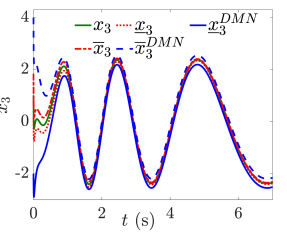
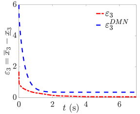
Figure 1: State, $x_{3}$, as well as its upper and lower framers and error returned by our proposed observer, $\overline{x}_{3},\underline{x}_{3},\varepsilon_{3}$, and by the observer in [20], $\overline{x}^{DMN}_{3},\underline{x}^{DMN}_{3},\varepsilon^{DMN}_{3}$ for the CT System example.

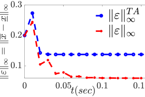
Figure 2: State, $x_{2}$, and its upper and lower framers, returned by our proposed observer, $\overline{x}_{2},\underline{x}_{2}$, and by the observer in [3], $\overline{x}^{TA}_{2},\underline{x}^{TA}_{2}$ (left) and norm of framer error (right) for the DT System example.

VI Conclusion and Future Work

A novel unified approach to synthesize interval-valued observers for bounded-error locally Lipschitz nonlinear continuous-time (CT) and discrete-time (DT) systems with nonlinear noisy observations was presented. The proposed observer was shown to be correct by construction using mixed-monotone decompositions, i.e., the true state trajectory of the system is guaranteed to be framed by the states of the observer without the need for additional constraints or assumptions. Moreover, we provide semi-definite programs for both CT and DT cases to find input-to-state stabilizing observer gains that are proven to be optimal in the sense of $\mathcal{H}_{\infty}$. Finally, simulation results demonstrated the better performance of the proposed interval observers when compared to some benchmark CT and DT interval observers. Designing hybrid interval observers and considering unbounded unknown inputs will be considered in our future work.

References

• [1] Y. Wang, D. Bevly, and R. Rajamani. Interval observer design for LPV systems with parametric uncertainty. Automatica, 60:79–85, 2015.
• [2] S. Chebotarev, D. Efimov, T. Raïssi, and A. Zolghadri. Interval observers for continuous-time LPV systems with L1/L2 performance. Automatica, 58:82–89, 2015.
• [3] A.M. Tahir and B. Açıkmeşe. Synthesis of interval observers for bounded Jacobian nonlinear discrete-time systems. IEEE Control Systems Letters, 2021.
• [4] M. Khajenejad, Z. Jin, and S.Z. Yong. Interval observers for simultaneous state and model estimation of partially known nonlinear systems. In American Control Conference (ACC), pages 2848–2854, 2021.
• [5] M. Khajenejad and S.Z. Yong. Simultaneous input and state interval observers for nonlinear systems with full-rank direct feedthrough. In IEEE Conference on Decision and Control, pages 5443–5448, 2020.
• [6] L. Farina and S. Rinaldi. Positive linear systems: theory and applications, volume 50. John Wiley & Sons, 2000.
• [7] M. Kieffer and E. Walter. Guaranteed nonlinear state estimation for continuous-time dynamical models from discrete-time measurements. IFAC Proceedings Volumes, 39(9):685–690, 2006.
• [8] F. Cacace, A. Germani, and C. Manes. A new approach to design interval observers for linear systems. IEEE Transactions on Automatic Control, 60(6):1665–1670, 2014.
• [9] D. Efimov, T. Raïssi, S. Chebotarev, and A. Zolghadri. Interval state observer for nonlinear time varying systems. Automatica, 49(1):200–205, 2013.
• [10] M. Khajenejad, F. Shoaib, and S.Z. Yong. Interval observer synthesis for locally Lipschitz nonlinear dynamical systems via mixed-monotone decompositions. In American Control Conference (ACC), accepted. IEEE, 2022, https://arxiv.org/pdf/2202.11689.pdf.
• [11] M. Khajenejad and S.Z. Yong. Tight remainder-form decomposition functions with applications to constrained reachability and interval observer design. arXiv preprint arXiv:2103.08638, 2021.
• [12] M. Abate, M. Dutreix, and S. Coogan. Tight decomposition functions for continuous-time mixed-monotone systems with disturbances. IEEE Control Systems Letters, 5(1):139–144, 2020.
• [13] L. Yang, O. Mickelin, and N. Ozay. On sufficient conditions for mixed monotonicity. IEEE Transactions on Automatic Control, 64(12):5080–5085, 2019.
• [14] H.K. Khalil. Nonlinear systems. Upper Saddle River, 2002.
• [15] G.R. Duan and H.H. Yu. LMIs in Control Systems: Analysis, Design and Applications. CRC press, 2013.
• [16] E.D. Sontag and Y. Wang. New characterizations of input-to-state stability. IEEE Trans. on Automatic Control, 41(9):1283–1294, 1996.
• [17] R.J. Plemmons. M-matrix characterizations. I: nonsingular M-matrices. Linear Algebra and its Applications, 18(2):175–188, 1977.
• [18] F. Mazenc and O. Bernard. When is a matrix of dimension 3 similar to a Metzler matrix application to interval observer design. IEEE Transactions on Automatic Control, pages 1–1, 2021.
• [19] J.F. Sturm. Using SeDuMi 1.02, a MATLAB toolbox for optimization over symmetric cones. Optimization methods and software, 11(1-4):625–653, 1999.
• [20] T.N. Dinh, F. Mazenc, and S. Niculescu. Interval observer composed of observers for nonlinear systems. In European Control Conference (ECC), pages 660–665. IEEE, 2014.
• [21] D. Efimov, W. Perruquetti, T. Raïssi, and A. Zolghadri. On interval observer design for time-invariant discrete-time systems. In European Control Conference (ECC). IEEE, 2013.