Graph-Survival: A Survival Analysis Framework for Machine Learning on Temporal Networks

Abstract

Continuous time temporal networks are attracting increasing attention due their omnipresence in real-world datasets and they manifold applications. While static network models have been successful in capturing static topological regularities, they often fail to model effects coming from the causal nature that explain the generation of networks. Exploiting the temporal aspect of networks has thus been the focus of various studies in the last decades.

We propose a framework for designing generative models for continuous time temporal networks. Assuming a first order Markov assumption on the edge-specific temporal point processes enables us to flexibly apply survival analysis models directly on the waiting time between events, while using time-varying history-based features as covariates for these predictions. This approach links the well-documented field of temporal networks analysis through multivariate point processes, with methodological tools adapted from survival analysis. We propose a fitting method for models within this framework, and an algorithm for simulating new temporal networks having desired properties. We evaluate our method on a downstream future link prediction task, and provide a qualitative assessment of the network simulations.

Keywords Temporal Networks, Survival Analysis, Link Prediction

1 Introduction

The study of continuous time temporal networks have attracted growing interest in the past decades, as time-stamped relational data emerges from various sources, including e-mail communication, e-commerce, or even neuron firing data [12, 9]. Example of use-case includes the study opinion dynamics, epidemic spreading, and recommender systems. Previous attempt to model such networks have traditionally relied on a discretization of time, allowing the representation of the temporal graph as a discrete sequence of static graphs [14, 13, 8]. As described in [16], these attempts to read this problem through the well documented lens of graph theory fails to capture mechanisms coming from the causal nature of temporal networks. Moreover, temporal relational data is often available with a high level of time granularity, allowing us to consider the time-stamps as continuous [25]. The interaction patterns are often heavily localized in time, exhibiting a property commonly known as burstiness [19]. Thus, one of the challenges in temporal network modelling is to find assumptions that allow explaining the observed burstiness. For instance, a good model for temporal social networks should be able to give an idea of the duration that will separate two interactions between users, given a certain historical context. To this date, few tools are available for continuous time temporal network analysis, notably methods coming from computational social sciences [5], or from point process modelling [2]. On the other hand, Survival Analysis has proven successful in the study of time-to-event data [1], and nowadays, a broad range of tools is available for it [3]. In order to make these tools applicable to temporal networks, we propose to apply Survival Analysis to the waiting times between events for each dyad. This method allows to elegantly and flexibly include inductive bias, in order to assess the statistical properties of an observed temporal graph, and predict the future interactions. A visual summary of our method can be seen on Figure 1. The inter-event times are modelled using survival analysis conditioned on the time-varying features, in order to incorporate a first order dependency of the hazard rate on the history.

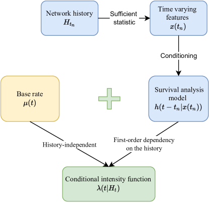
Figure 1: Summary of the Graph-Survival framework

Our main contributions are as follows:

1. We introduce Graph-Survival: a framework that allows to translate any survival analysis model on a generative temporal network model. This framework allows including modelling assumptions on the inter-arrival times between event for each edge, in order to measure the salience of temporal network properties in observed data, and to predict the evolution of the network.

2. We propose an algorithm for simulating networks based on this framework. This algorithm allows reproducing synthetically properties observed in real-world network, such as burstiness.

3. We show how to perform Maximum Likelihood Estimation of model parameters on an observed dataset, and evaluate the quality of the fitting on a downstream link prediction task.

4. For reproducibility purposes, we provide an open-source implementation of our method (<github url here>)

Outline

In section 2 we give a brief introduction to the theoretical notions used in the Graph-Survival framework. In 3 we introduce the framework, including the form of the likelihood and the simulation algorithm. In 4 we give some examples of models within this framework. In 5 we assess the performances of our method through numerical experiments.

2 Background on Temporal Networks and Survival Analysis

In this section we provide an overview of temporal networks, survival analysis and point processes. We then show how to design a first order Markov chain model for temporal network, given a survival analysis model for the edge inter-arrival times.

2.1 Temporal networks

Let $\mathcal{U}$ and $\mathcal{V}$ denote a set of source and destination nodes respectively, $\mathcal{E}\subset\mathcal{U}\times\mathcal{V}$ the set of possible edges. Temporal network data takes the form of a sequence of time-stamped network events $\mathcal{H}=\{w_{m}=(e_{m},t_{m})|m=1,...,M\}$, where $M$ is the number of events, $0<t_{1}<...<t_{M}$ is an ordered sequence of pairwise distinct, positive time stamps, $e_{m}=(u_{m},v_{m})\in\mathcal{E}$ is the edge involved in the $m$-th event, and $u_{m}\in\mathcal{U}$ and $v_{m}\in\mathcal{V}$ are the source and destination nodes respectively. For instance, each event $((u,v),t)$ can represent a message sent by user $u$ to user $v$ at time $t$. For any time $t$ we will denote $\mathcal{H}_{t}=\{w_{m}\in\mathcal{H}|t_{m}<t\}$ the history of the network up to time $t$. Moreover, for any edge $e=(u,v)\in\mathcal{E}$, we denote $\mathcal{H}^{(e)}=\{w_{m}\in\mathcal{H}|e_{m}=e\}$ the history of events involving the edge $e$. Finally, we denote by $\mathcal{H}_{t}^{(e)}$ the history of events involving the edge $e$, up to time $t$.

2.2 Survival Analysis

Survival Analysis is the study of time-to-event data. It has been traditionally used in the medical field to model the expected survival time of patients under different setups, for instance the treatments provided or the pre-conditions of the patient [1]. One of the goals of Survival Analysis is to quantify the effect of input covariates on the risk for a given event to happen. Such studies are often conducted in the presence of censored data, meaning that the time-to-event is not directly known, but we have access to a lower/upper bound instead. A mathematical object that is central in survival analysis is the hazard function, denoted $h$. This function is such that for any positive real value time $t\in[0,+\infty[$, the probability for the event of interest (e.g. death of the patient) to happen in an infinitesimal interval $[t,t+dt[$, conditional on this event not occurring before $t$, is equal to $h(t)dt$. It can be shown that the probability for the event to happen only after $t$ (also framed survival function), is equal to $S(t)=\exp(-\int_{0}^{t}h(s)ds)$. Unlike the probability density function or the survival function, the hazard function only has the constraint that it should be strictly positive. As a consequence it appears as a convenient tool to design statistical models on the survival time, conditioned on individual-specific covariates.

2.3 Temporal Point Processes

Temporal point processes are random variables whose realizations are sets of positive, real-valued time-stamps. A fundamental quantity in the study of temporal point processes is the conditional intensity function, denoted $t\mapsto\lambda(t|\mathcal{H}_{t})$, such that for any $t\in[0,+\infty[$, $\lambda(t|\mathcal{H}_{t})dt$ measures the average number of events occurring in the interval $[t,t+dt[$, given the event history up to time $t$ [7]. In the case of Poisson processes, the conditional intensity function is independent of the history, meaning that it is a deterministic function: $\lambda(t|\mathcal{H}_{t})=\lambda(t)$. In contrast, self-exciting processes are governed by a stochastic conditional intensity function, whose value at time $t$ depends on the samples previous to $t$. While Poisson Processes can be accurate when we have a clear a priori idea of the form of the intensity function, they are unable to adapt to new events. On the contrary self-exciting processes allow the conditional intensity function to take into account past events.

2.4 From survival analysis model to first order Markov chain

By supposing that the successive inter-arrival times are governed by a survival analysis model, we can construct a first order Markov chain.

To do so, we suppose that in absence of any event, the point process is generated by a deterministic base intensity $\lambda(t|\mathcal{H}_{t}=\emptyset)=\mu(t)$. We also suppose the existence of a vector-valued stochastic function $t\mapsto\bm{x}(t)$, defined for any time $t\in[0,+\infty[$, called time-varying features. Then, given a non-empty history of previous events $\{t_{1},...,t_{n}\}$, we suppose that $\bm{x}(t_{n})$is a sufficient statistic of the history up to time $t_{n}$, for the prediction of the next event: $\lambda(t|\mathcal{H}_{t}=\{t_{1},...,t_{n}\})=\lambda(t|\bm{x}(t_{n}))$. Next we posit a survival model on the $n$-th inter-arrival time, $\tau_{n}=t_{n+1}-t_{n}$, conditioned on the feature vector $\bm{x}(t_{n})$:

Definition 2.1.

We define the transition hazard rate as the hazard rate in the model of the next event given the features at the time of the previous event. We denote it $\tau\mapsto h(\tau|\bm{x}(t_{n}))$. Here the notation $\tau$ is used to specify that we are considering the time since the last event.

This means that the conditional intensity function, conditional on a non-empty history, is equal to

$$\lambda(t|\mathcal{H}_{t}=\{t_{1},...,t_{n}\}\})=h(t-t_{n}|\bm{x}(t_{n}))$$

Alternatively, the occurrence of each new event can be seen as incrementing the conditional intensity function with a time-varying value:

Definition 2.2.

We define on $[0,+\infty[$ the intensity increment function:

$$t\mapsto\gamma(t|\mathcal{H}_{t})=h(t-t_{n}|\bm{x}(t_{n}))-\mu(t)$$

While $h$ is a deterministic function of the time elapsed since the last event, $\gamma$ is a stochastic function of the absolute time of the process. Since $\gamma$ depends on the history $\mathcal{H}_{t}$ only through the time-varying feature vector $\bm{x}(t_{n})$, we will use the notation $\gamma(t|\mathcal{H}_{t})=\gamma(t|\bm{x}(t_{n}))$.

Conditioned on the feature function $\bm{x}$, the procedure defined here defines a self-exciting process, where the intensity function gets set to the value of the hazard function at every new event.

Proposition 2.1.

The conditional intensity function of the point process defined above is given for any $t\in[0,+\infty[$ by

$$\lambda(t|\mathcal{H}_{t})=\mu(t)+\sum\limits_{t_{n}<t}\mathbbm{1}_{t\in]t_{n+1},t_{n}]}\gamma(t|\mathcal{H}_{t})$$

where $\mathbbm{1}_{t\in]t_{n+1},t_{n}]}$ is the indicator function asserting that the current time is before the next event.

This formulation is reminiscent of Hawkes processes [10], with a difference being that here we make use of time-varying features, and make use only of the last event to predict the next one, while Hawkes processes add a time-varying increment for each previous event in the history.

To summarize, here we show how to start from a survival analysis model, represented by a modelled hazard function, and derive a model for the conditional intensity function of a given point process.

3 The Graph-Survival framework

In this section we show how to apply the previous procedure to derive a temporal graph generative model, given a survival analysis model.

3.1 General Description

3.1.1 Form of the edge intensity function

In our framework, given a temporal network such as the one described in 2.1, we propose to consider for each edge $e=(u,v)\in\mathcal{E}$, the point process generating the edge-specific history $\mathcal{H}_{e}$.

Definition 3.1.

For each edge $e\in\mathcal{E}$ we define the edge-wise conditional intensity function $t\mapsto\lambda^{(e)}(t|\mathcal{H}_{t})$, associated to the point process generating the edge history $\mathcal{H}^{(e)}$

Note that here we allow the edge-wise conditional intensity function to be conditioned on the history of the whole network, and not only on the edge-wise history $\mathcal{H}_{t}^{(e)}$.

We propose to posit a model such as the one described in 2.4 on each of the edge-wise intensity functions. To do this, we define a time-varying feature function $\bm{x}:t\mapsto\bm{x}(t|\mathcal{H}_{t})\in\mathbb{R}^{|\mathcal{E}|\times D}$, that allows, for any edge $e$ and time $t$, to access an array of features $\bm{x}^{(e)}(t|\mathcal{H}_{t})\in\mathbb{R}^{D}$, where D is the number of features. We provide examples of such edge features in section 3.2

Then, applying the procedure in 2.4, we define the edge conditional intensity function as

$$\lambda^{(e)}(t|\mathcal{H}_{t})=\mu^{(e)}(t)+\sum\limits_{t_{n}<t}\mathbbm{1}_{t\in]t_{n+1},t_{n}]}\gamma^{(e)}(t|\bm{x}^{(e)}(t|\mathcal{H}_{t})).$$

Based on this formulation, we can parameterize the base rate and the intensity increment function, yielding a fully parametric model of the temporal network history. Note that a non-parametric form of the conditional intensity function could also be considered.

3.1.2 Loss function

Supposing a parameterization of the intensity function above, we propose to find the maximum likelihood estimates of the parameters by optimizing the negative log-likelihood.

Given a point process model with conditional intensity $\lambda(t|\mathcal{H}_{t})$, the general form of the likelihood of an observed event history $\left\{t_{1},...,t_{n}\right\}$ on an interval $[0,T]$ is derived in [7] and given by

$$p(\left\{t_{1},...,t_{n}\right\})=\left(\prod\limits_{i=1}^{n}\lambda(t_{i}|\mathcal{H}_{t})\right)\exp\left(-\int\limits_{0}^{T}\lambda(s|\mathcal{H}_{s})ds\right).$$

We use the independence property of the edges conditional on the time varying features to define the the negative log-likelihood of the model:

Definition 3.2.

The negative log-likelihood of our network point process model is given by

$$L(\mathcal{H})=\sum\limits_{e\in\mathcal{E}}\int\limits_{0}^{T}\lambda^{(e)}(s|\mathcal{H}_{s})ds-\sum\limits_{i=1}^{|\mathcal{H}^{(e)}|}\log\left(\lambda^{(e)}(t|\mathcal{H}_{t})\right).$$ (1)

Alternatively, this loss function can be reindexed as a sum indexed by the events, since we have $L(\mathcal{H})=L_{(pos)}(\mathcal{H})+L_{(neg)}(\mathcal{H})$ with:

• $L_{(neg)}(\mathcal{H})=\sum\limits_{w_{m}\in\mathcal{H}}\left(\sum\limits_{e\in\mathcal{E}}\int\limits_{t_{m-1}}^{tm}\lambda^{(e)}(s|\mathcal{H}_{s})ds\right)$

• $L_{(pos)}(\mathcal{H})=\sum\limits_{w_{m}\in\mathcal{H}}-\log(\lambda^{(e_{m})}(t|\mathcal{H}_{t}))$

To get to this expression we split the integral on the left hand side of 1 over the inter-arrival time interval $\{[t_{m-1},t_{m}[,m=1,...,M\}$, and we re-index the terms by event.

Although the edge sum necessary to compute $L_{(neg)}(\mathcal{H})$ leads to a computational complexity proportional to the square of the number of nodes, the loss function can be approximated by sampling a set of contrastive edge samples $\tilde{\mathcal{E}}_{m}$ for each event $m$, such that $|\tilde{\mathcal{E}}_{m}|\ll|\mathcal{E}|$. We can then substitute the full sum with the renormalized mean of their associated survival terms to approximate $L(\mathcal{H})\approx\tilde{L}_{(neg)}(\mathcal{H})+L_{(pos)}(\mathcal{H})$ with

$$\tilde{L}_{(neg)}=\sum\limits_{w_{m}\in\mathcal{H}}\frac{|\mathcal{E}|}{|\tilde{\mathcal{E}}_{m}|}\sum\limits_{e\in\tilde{\mathcal{E}}_{m}}\int\limits_{t_{m-1}}^{tm}\lambda^{(e)}(s|\mathcal{H}_{s})ds).$$

This approximated loss function has a number of terms proportional to the number of events in the network history. It can be further approximated computing it on batches, formed by taking slices of the history.

3.2 Features

As mentionned in the previous secion, out method can be implemented by carefully designing time-varying features on the network. Features that are traditionally used for heuristic-based link prediction include for instance the degrees of the involved nodes, the number of common neighbors. We derive a time-decaying version of these features, in order to down-weight the effet of events that occured a long time ago, in the feature values.

3.2.1 Examples of features

As is common in network analysis, the choice of features is highly dependent on the nature of the network considered, and the type of analysis being conducted. In a variety of previous work, some time-varying edge features have been introduced [5] [26] [4]. We provide three examples of time-decaying features. Here we denote by $\mathcal{H}_{t}^{u}$ the history of events involving node $u$, and $\gamma$ a decay hyper parameter controlling the rate at which the feature contributions from previous events ecome obsolete.

• The exponentially down weighted degree, defined at time $t$ for any node $u$ as

  $$deg(u,t;\gamma)=\sum_{(e_{m},t_{m})\in\mathcal{H}_{t}^{u}}exp(-\gamma_{1}(t-t_{m})).$$

  This feature quantifies the volume of interactions involving the node $u$, weighted by an exponentially decaying factor favoring recent interactions over old ones.

• The exponentially down weighted volume of interaction

  $$volume(e,t;\gamma_{3})=\sum_{\begin{subarray}{c}(e_{m},t_{m})\in H_{t}\end{subarray}}\exp(-\gamma(t-t^{\prime})).$$

  This feature measures the volume of recent interactions between the nodes involved in the edge $e$.

• The exponentially down-weighted number of common neighbors is calculated as

  $$cn(e,t)=\sum\limits_{v\in CN(e,t)}\exp(-\gamma(t-t_{last}(e,v))).$$

  Where $CN(e,t)$ is the set of common neighbors of the edge $e$ at time $t$ and $t_{last}(e,v)$ is the time of the last interaction between the nodes involved in $e$ and the common neighbor $v$.

3.2.2 Feature computation

As can be seen in 3.2.1, in many cases the computation of the feature vector only requires storing a number $O(|U|+|V|)$ of variables, in order to make the feature vector accessible for any edge-time pair Since the feature function takes value in a space of dimension $|\mathcal{U}|\times|\mathcal{V}|\times D$, its explicit computation for all the events and non-events is unfeasible for reasonable-sized networks. Instead, for the features that we consider in this paper, we can store an array of smaller-dimensional time-varying statistics $\left\{g_{1},...,g_{n}\right\}$ of the network, such that for any edge, its associated feature vector can be computed at any time: $\bm{x}^{(e)}(t)=F_{e}({g_{1}(t),...,g_{S}(t)})$ where $F_{e}$ is a simple transformation.

For instance, the computation of the number of common previous neighbors between two nodes $u$ and $v$ at a time $t$ can be done simply by keeping in memory the set of previous neighbors for each node, and comparing the two sets at the given time.

3.3 Simulation

Here we show how to use our model to generate synthetic networks. This simulation method is based on Ogata’s modified thinning algorithm [20]. Here we provide a brief explanation of this method. For every edge $e$, we remind that $t\mapsto\lambda^{(e)}(t|\mathcal{H}_{t})$ denotes the conditional intensity of the point process of edge $e$. Similarly, we define $\lambda$, the total conditional intensity function, that generates the sequence of event times in the network:

$$t\mapsto\lambda(t|\mathcal{H}_{t})=\sum\limits_{e\in\mathcal{E}}\lambda^{(e)}(t|\mathcal{H}_{t}).$$

We start from an initial time $t_{0}$. At each iteration, we compute a local upper-bound of the total intensity on a right neighborhood of the current time. This upper-bound allows us to generate the next event time across the network, in a rejection sampling manner. To do so, we generate a sample from an exponential distribution with rate parameter equal to the upper-bound, and then accept this sample with a probability proportional to the total intensity value at the newly generated time.

Once this new event time is generated, we attribute it to an edge randomly using a multinomial distribution over the set of possible edges. The probability for each edge to be selected is proportional to their intensity value at this new sample. We summarize this method in Algorithm 1

Input: initial time $t_{0}$, upper bound $T$, maximum number of iterations $N$

Initialize $s=t_{0}$, $\mathcal{H}_{sample}$.

while $s>T$ or $n>N$ do

$\lambda^{(\star)}=\sup_{s>t}\lambda(s|\mathcal{H}_{s})$

Sample $w\sim Exponential(\lambda^{(\star)})$

Set s = s+w

      Sample $U\sim Uniform([0,1])$

      if $U\leq\frac{\lambda(s)}{\lambda^{(\star)}}$ then

            

Define for each edge $e$ the probability

$$p^{(e)}=\frac{\lambda^{(e)}(s|\mathcal{H}_{s})}{\sum_{e^{\prime}\in\mathcal{E}}\lambda^{(e^{\prime})}(s|\mathcal{H}_{s})}$$

Sample $\tilde{e}\sim Multinomial(1,\{p_{e}|e\in\mathcal{E}\})$

            Add the event $(\tilde{e},s)$ in $\mathcal{H}_{sample}$

            Set $n=n+1$

       end if

      

end while

Algorithm 1 Simulation using the Ogata’s modified thinning method

4 Examples of models

In order to illustrate our framework, we propose two examples of simple models that follow the construction presented above.

4.1 Edge Poisson Process

As a first baseline, we consider that each edge history is independently generated by a Poisson Process, meaning that the rates are independent of the network history. Whithout including prior knowledge on the temporality of the edge base rate, a simple way of doing it is to define the constant Poisson Rate of the edge $e=(u,v)$ as:

$$\mu_{poisson}^{e}\overset{\Delta}{=}h(2c+\alpha_{u}+\alpha_{v}-d(z_{u},z_{v}))$$ (2)

Where for each node $u\in\mathcal{U}\cup\mathcal{V}$, $\alpha_{u}\in\mathbb{R}$ is a sociality coefficient, $z_{u}\in\mathbb{R}^{d}$ is an embedding of dimension $d$, $c$ is an offset parameter, $h$ is an activation function, and $d$ is a distance function. In our example we use the softplus function $h(x)=log(1+exp(x))$. This model for the rate is inspired by the literature about latent space models for graphs [11]. The underlying intuition is that each node $u\in\mathcal{U}$ in the network is equipped with a position $z_{u}$ in a latent social space, and a disk $B_{u}$ centered around $z_{u}$ and with radius $\alpha_{u}+c$, such that two nodes $u$ and $v$ have a positive log-odd of interaction whenever $B_{u}\cap B_{v}$ is non-empty. In equation 2, the smaller $d(z_{u},z_{v})$ is, the higher the Poisson rate between $u$ and $v$ will be.

4.2 First-order Markov Chain

Whereas the Poisson model yields an intensity function that is independent of the past network history, we propose to include a simple interaction between the past of the network and the next event by constructing a Markov Chain following the procedure in 3.1.1. Here we temporarily omit the edge subscript, for notation simplicity. As a base rate, we choose to use the Poisson Rate defined above. For the transition survival model, we rely on a recent work [3] that defines the hazard function as a piece-wise constant one:

$$\forall\tau>0,h(\tau|x(t_{n}))=\sum_{j=1}^{J}\mathbbm{1}_{I_{j}}(\tau)\exp(\theta_{j}^{T}x_{t_{n}}).$$

Thus, the conditional intensity function is given by

$$\lambda(t)=\mu_{poisson}+\mathbbm{1}_{t>t_{n}}\gamma(t|x(t_{n})).$$

Where $t_{n}$ is the time of the previous event for the considered edge and $\gamma(t|x(t_{n}))\overset{\Delta}{=}h(t-t_{n}|x(t_{n}))$.

To summarize, in the case of the Poisson rate we drop the time-dependence of the edge events, and specify their rate as a constant that depends only on inner properties of the edges, such as their sociality coefficient or their embeddings. In the first order Markov model, the event time of the next event for a considered dyad, is modelled by conditional on the edge feature values at the last event time for this dyad.

5 Evaluation

We evaluate our method in two ways. First we assess its ability to generate realistic networks. Second, we assess its predictive capacity through a downstream Link Prediction task.

5.1 Datasets

We work with two real-world datasets, the Irvine College Message Dataset and the Enron Dataset. The Irvine College Message Dataset (framed CollegeMsg here) is a publicly available dataset (https://snap.stanford.edu/data/CollegeMsg.html) composed of 59835 directed interactions between students in an online social media platform in the University of California, Irvine, on a total time-span of 193 days. While this dataset has been studied in previous work [21] to measure the evolution of some topological properties of the network, here we focus on the temporal aspect of edge-specific point process realization. The Enron Dataset (Enron), publicly available on https://www.cis.jhu.edu/~parky/Enron/ contains 125409 directed message sent between employees of the company Enron between 1999 and 2003.

In our case we preprocess both datasets, by removing simultaneous events. This includes for instance broadcasted e-mails that are present in large amounts in the Enron dataset, or duplicate events in general. For the Enron Dataset we obtain a final dataset of 4529 links, while we filter the CollegeMsg Dataset to keep only the 20000 first interaction.

Dataset	Number of temporal events	Directed
Enron	4529	Yes
CollegeMsg	20000	Yes

Table 1: Properties of the datasets

5.2 Implementation

We implement our method using Pytorch, in order to benefit from automatic differentiation. Our implementation is composed of two separate modules. One module is the intensity function, that takes as input tuples composed of edges, interaction times, time histories and feature values, and provide as an output a positive real-valued score. The NLLLoss takes as input the intensity values and the interaction times and computes the value of the negative log likelihood define in 1. This implementation allows us to benefit from automatic differentiation. We use the AdamW optimization method [17]. This allows us to ensure fast convergence to an optimum of both embeddings and linear parameter, while controlling over-fitting of the embeddings by adjusting the weight decay parameter. In our experiments we set the learning rate to 0.8 and the weight decay to 0.9. For the Poisson base rate we use embeddings of dimension 20. For the piece-wise constant hazard of the First-order Markov model, we select cut-off points for based on the inter-arrival time distribution of the dataset at the network level.

5.3 Simulation

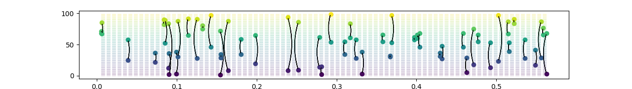
Figure 2: First 50 events on our simulated network

We evaluate the ability of our framework to generate realistic network histories. Real-world temporal networks, along are characterized by a fundamental property called burstiness.

The burstiness measure defined in [19] is defined as follows, for a given time history $t_{1},...,t_{n}$. First, one measures the coefficient of variation of the inter-arrival times $\tau_{i}=t_{i+1}-t_{i},i=1,...,n-1$ :

$$cv=\sqrt{\frac{\sum{(\tau_{i}-\bar{\tau})^{2}}}{(n-1)*\bar{\tau}^{2}})}$$

Where $\bar{\tau}$ is the mean inter-arrival time for this sequence.

This value is equal to 1 for a Poisson Process, 0 for if the history is periodic (i.e. the inter-event times are all the same). Long tail inter-arrival distribution tipycally yield large values for this coefficient of variation.

In order to obtain a score in the interval $[-1,1]$, previous autors have proposed to normalize the coefficient of variation, defining the burstiness score:

$$B=\frac{cv-1}{cv+1}.$$

This one has values close to 0 for Poisson processes, -1 for periodic sequences, and close to 1 for very bursty sequences. In our experiment, we simulated a network history using the time decaying feature defined above and a Markov model. Then we compute for each edge the burstiness of the associated event sequence. Finally we plot the histogram of the obtained burstinesses, expecting a number of bursty event sequences.

We simulate a network using the first order Markov model and the exponentially downweighted features defined above, and plot the histogram of the burstinesses associated with the various edges.

We visualize the obtained simulation on Figure2.

Figure 3 shows the resulting histogram of burstiness. We see that the range $[0,1[$ is fairly well populated, meaning that our simulation allows to generate partially the burstiness observed in real-world data. For comparison, we plot on Figures 4 and 5 the burstinesses of the Enron dataset(a corporate e-mail dataset), and on the College Msg dataset respectively. In their case, the bursty behavior of the edges in the network can be noted since a good amount of edges have a burstiness coefficient between $0$ and $1$.

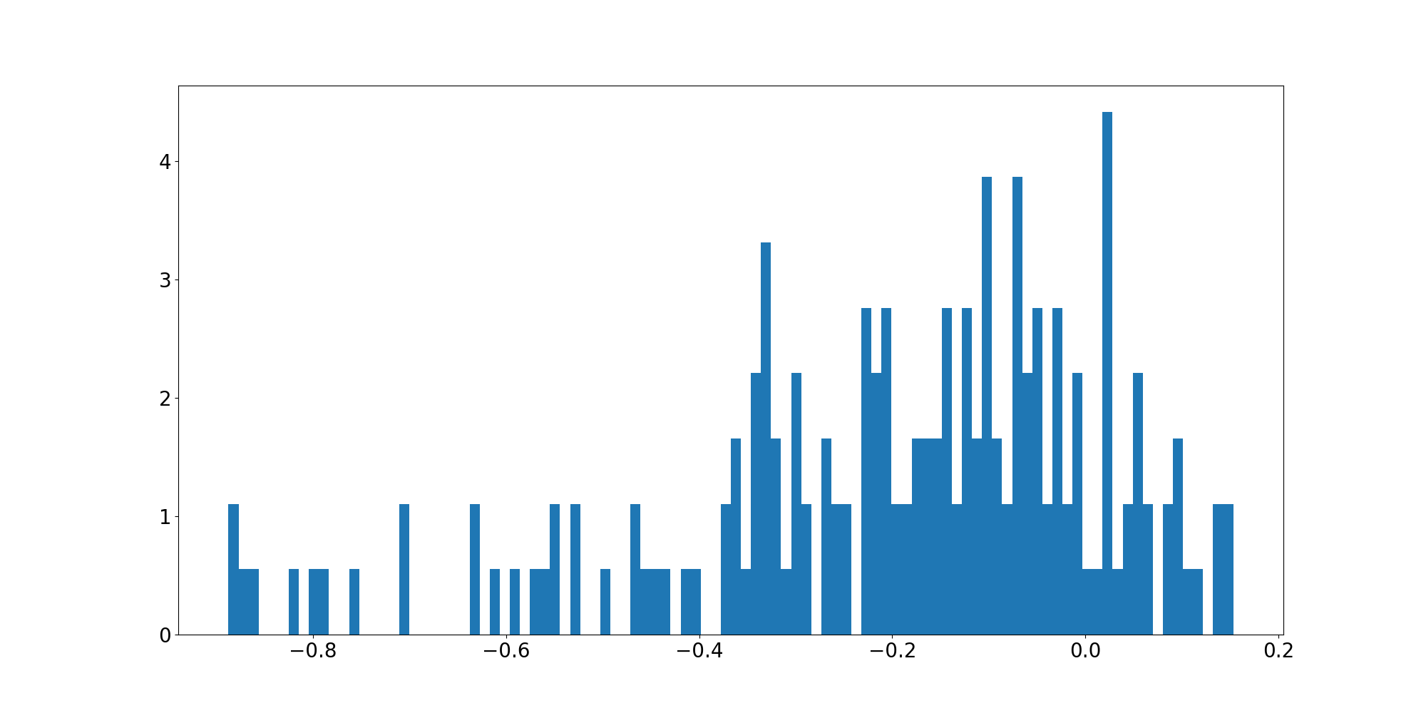
Figure 3: Burstiness histogram on our simulated network

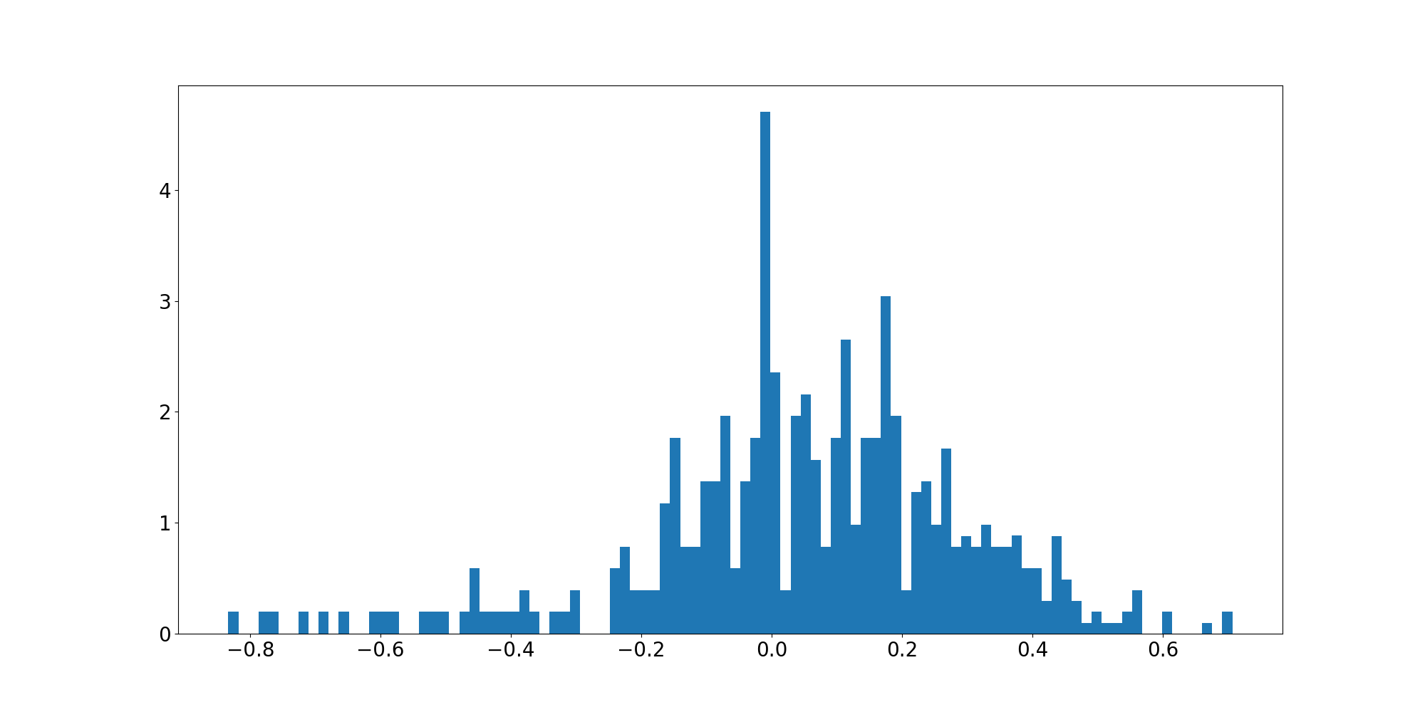
Figure 4: Burstiness histogram on the Enron dataset

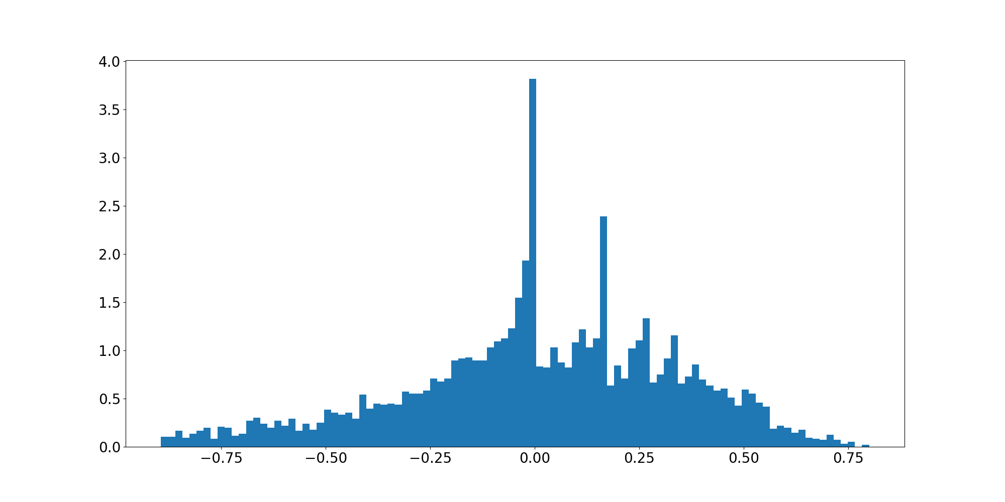
Figure 5: Burstiness histogram on the Irvine College Message Dataset

5.4 Future Link Prediction

5.4.1 Task Description

We assess the predictive ability of our model by performing a Future Link Prediction task. More specifically, we split the history in two parts, and train the models on the first slice of history. For events in the test part of the history, we try predict the destination node based on the observed source node.

5.4.2 Train-Test splitting and preprocessing

In order to split the network history we pick three cut-off times $0<t_{train}<t_{val}<t_{test}$ and split the history into three sub-sets: the train history $\mathcal{H}_{train}=\{w_{m}\in\mathcal{H},t_{m}\in[0,t_{train}]\}$, the validation history $\mathcal{H}_{val}=\{w_{m}\in\mathcal{H},t_{m}\in[t_{train},t_{val}]\}$, and the test history $\mathcal{H}_{test}=\{w_{m}\in\mathcal{H},t_{m}\in[t_{val},T]\}$.

For each train event in $w=((u,v),t)\in\mathcal{H}_{train}$, we sample $n=1$ a negative neighbor $\bar{v}\in\mathcal{V}\backslash\{u,v\}$ and define a negative event $\bar{w}=((u,\bar{v}),t)$. We introduce target variables $y=1$ and $\bar{y}=0$ for the positive and negative event respectively. Using this procedure we obtain a labelled dataset

$$\mathcal{D}={(w_{1},y_{1}),...,(w_{n},y_{n})}.$$

We treat the hazard models defined above as score functions :$f:w=(e,t)\mapsto f(w)\in\mathbb{R}_{+}$. Finally we use the AUC metric to measure the ability of a given score function to separate positive and negative samples.

5.4.3 Baselines

We compare 4 different prediction methods:

• The Poisson model (4.1), assuming a constant intensity in time.

• The Markov survival model endowed with a piece-wise hazard, thus including a first order dependency in the history.

• The preferential attachment: this one uses the product of the degrees of the nodes at a given time as a predictor for their probability of forming an edge. This heuristic has been shown in [18] to yield good prediction results compared to state-of-the art baselines.

• A random intensity value for any given node pair.

The ROC curves for both of the datasets are shown in Figures 6 and 7.

We summarize the results in table 2

Model	Enron	CollegeMsg
Poisson	0.6115	0.6568
Preferential Attachment	0.6625	0.7499
Random	0.5153	0.5026
Markov-PWC	$\boldsymbol{0.8306}$	$\boldsymbol{0.7665}$

Table 2: Future Link Prediction Accuracies for different Datasets

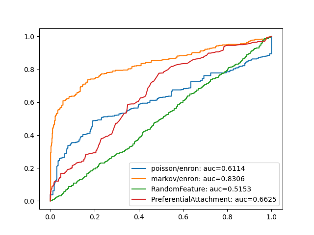
Figure 6: ROC Curve for the Enron dataset

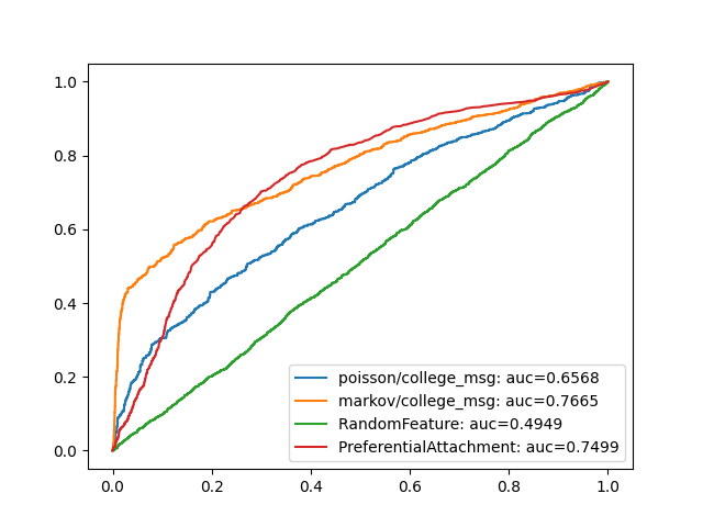
Figure 7: ROC Curve for the Irvine College Message dataset

On both datasets, our method (the blue curve on Figure 6 and 7) performs better prediction AUC that the other methods. The gap in prediction is especially large for small intensity threshold values. It can be seen that methods that the first order Markov and the Preferential Attachment methods perform better than the constant rate method and the Random Feature. This is due to their ability to incorporate time-varying effects in the predictions.

6 Related Work

To our knowledge, the previous work that comes closest to the present method is the one presented in [22]. In this one, the authors propose to posit a mutually exciting model between the different edges, such that the interactions occurring for a given edge influence the ones coming occurring on neighboring edges. However, they rely mostly on time-varying node embeddings to define the conditional intensity functions, while in our case we rely on static embedding and rely on time-varying features to model the time-evolution of the intensity.

Another closely related line of research uses deep learning to infer embedding trajectories in a latent space[15, 24, 27, 6]. While this line of research already yields promising results on future link prediction or temporal node classification on very large scale networks, smaller size networks don’t necessarily contain the information necessary to train time-varying embeddings.

Finally, former work coming from computational social sciences also propose to model temporal networks through their intensity functions, in order to assess the effect of the temporal network topology on the rates of link formation [5, 4, 23]. Specifically, relational event modelling also rely on a piece-wise constant intensity hypothesis to define the likelihood of the observed network. In our case, we provide more flexibility by allowing to posit a custom hazard function on the edge-inter-event times, and making it dependent or not of the evolution of other edges in the network, depending on the specific needs.

7 Conclusion

We have introduced Graph-Survival, a framework that allows to translate survival analysis models into generative models for temporal networks. Using a survival analysis model on the inter-arrival times is a simple and elegant way of capturing the influence of the temporal network topology on the intensity of the dyadic point processes. Our proposed framework suggests that by encoding the past history in an appropriate vector of sufficient statistics, one can very simply include inductive bias on the time-evolution of the network, and use the resulting model for prediction or simulation. We empirically demonstrated that a simple example of model in our framework is able to generate bursty network histories, and perform accurate future link prediction.

In further work we plan to further integrate representation learning as a substitute for the hand-crafted features, while investigating the effects of higher-order history dependency on the quality of the model.

References

- [1] Aalen, O., Borgan, O., and Gjessing, H. Survival and Event History Analysis: A Process Point of View. 01 2008.
- [2] Bacry, E., Bompaire, M., Deegan, P., Gaïffas, S., and Poulsen, S. V. tick: a python library for statistical learning, with an emphasis on hawkes processes and time-dependent models. Journal of Machine Learning Research 18, 214 (2018), 1–5.
- [3] Bender, A., RÃŒgamer, D., Scheipl, F., and Bischl, B. A General Machine Learning Framework for Survival Analysis. 158–173.
- [4] Bois, C. D., Butts, C. T., and Smyth, P. Stochastic blockmodeling of relational event dynamics. Journal of Machine Learning Research 31 (2013), 238–246.
- [5] Butts, C. T. A relational event framework for social action. 155–200.
- [6] Dai, H., Wang, Y., Trivedi, R., and Song, L. Deep Coevolutionary Network: Embedding User and Item Features for Recommendation.
- [7] Daley, D., and Vere-Jones, D. An Introduction to the Theory of Point Processes Volume I, vol. I. 2010.
- [8] Durante, D., and Dunson, D. B. Locally adaptive dynamic networks. Annals of Applied Statistics 10 (2016), 2203–2232.
- [9] Goldenberg, A., Zheng, A. X., Fienberg, S. E., and Airoldi, E. M. A survey of statistical network models. 129–233.
- [10] Hawkes, A. G. Spectra of some self-exciting and mutually exciting point processes. Biometrika 58, 1 (1971), 83–90.
- [11] Hoff, P. D., Raftery, A. E., and Handcock, M. S. Latent space approaches to social network analysis. Journal of the American Statistical Association 97 (2002), 1090–1098.
- [12] Holme, P., and Saramäki, J. Temporal networks. Physics Reports 519 (10 2012), 97–125.
- [13] Kim, B., Lee, K., Xue, L., and Niu, X. A review of dynamic network models with latent variables *.
- [14] Krivitsky, P., and Handcock, M. A separable model for dynamic networks. Journal of the Royal Statistical Society. Series B, Statistical methodology 76 (01 2014), 29–46.
- [15] Kumar, S., Zhang, X., and Leskovec, J. Predicting dynamic embedding trajectory in temporal interaction networks. 1269–1278.
- [16] Latapy, M., Viard, T., and Magnien, C. Stream graphs and link streams for the modeling of interactions over time.
- [17] Loshchilov, I., and Hutter, F. Decoupled weight decay regularization. In International Conference on Learning Representations (2019).
- [18] Mara, A. C., Lijffijt, J., and Bie, T. D. Benchmarking network embedding models for link prediction: Are we making progress? Proceedings - 2020 IEEE 7th International Conference on Data Science and Advanced Analytics, DSAA 2020 (2020), 138–147.
- [19] Naoki Masuda, and Renaud Lambiotte. A Guide To Temporal Networks-World Scientific . 2016.
- [20] Ogata, Y. On Lewis’ Simulation Method for Point Processes. IEEE Transactions on Information Theory 27, 1 (1981), 23–31.
- [21] Panzarasa, P., Opsahl, T., and Carley, K. M. Patterns and dynamics of users’ behavior and interaction: Network analysis of an online community. Journal of the American Society for Information Science and Technology 60 (5 2009), 911–932.
- [22] Passino, F. S., and Heard, N. A. Mutually exciting point process graphs for modelling dynamic networks.
- [23] Perry, P. O., and Wolfe, P. J. Point process modelling for directed interaction networks. 821–849.
- [24] Rossi, E., Chamberlain, B., Frasca, F., Eynard, D., Monti, F., and Bronstein, M. Temporal graph networks for deep learning on dynamic graphs. 1–16.
- [25] Rozenshtein, P., and Gionis, A. Mining Temporal Networks. 3225–3226.
- [26] Vu, D. Q., Asuncion, A. U., Hunter, D. R., and Smyth, P. Dynamic egocentric models for citation networks. Proceedings of the 28th International Conference on Machine Learning, ICML 2011 (2011), 857–864.
- [27] Xu, D., Ruan, C., Korpeoglu, E., Kumar, S., and Achan, K. Inductive representation learning on temporal graphs. 1–19.