Geometry of Data

Abstract

Topological data analysis asks when balls in a metric space $(X,d)$ intersect. Geometric data analysis asks how much balls have to be enlarged to intersect.
We connect this principle to the traditional core geometric concept of curvature. This enables us, on one hand, to reconceptualize curvature and link it to the geometric notion of hyperconvexity. On the other hand, we can then also understand methods of topological data analysis from a geometric perspective.

1 Introduction

Many data sets come with a basic geometric structure, distances between data points. It is therefore natural to use geometric methods to analyze such data. The deepest geometric concepts, however, were developed in the 19th century for smooth manifolds, more precisely Riemannian manifolds. And the most fundamental concept there is curvature. In the 20th century, notions of curvature were successfully generalized to more general classes of spaces. Still, those spaces, like geodesic length spaces, are typically not discrete, in contrast to data sets. Thus, we have found it desirable to rethink fundamental geometric concepts from a more abstract perspective that also naturally includes discrete spaces. Of course, there are ideas and approaches that we can build upon, most importantly those pioneered by Gromov [21, 22]. From such a perspective, the distinction between discrete and connected spaces is partly one of scale. From a large scale perspective, spaces from those two classes may look alike.

Such a large scale perspective is still quantitative, hence geometric, and is therefore different from a qualitative topological approach. Nevertheless, as we shall see, there are important links between the two. In particular, we can look at the successful topological data analysis method of persistent homology from a geometric perspective.

Topological data analysis asks when balls in a metric space $(X,d)$ intersect. This is a qualitative concept, but the data analysis method of persistent homology makes this quantitative through the dependence on the radii of the balls. Geometric data analysis, as we conceive it in this contribution, asks how much balls have to be enlarged to intersect. And as we shall see, this is captured by a suitable concept of curvature. And curvature, from a general perspective as adopted here, quantifies convexity. Therefore, convexity and its strengthening as hyperconvexity will be our basic concepts.

2 Preliminaries from metric geometry

Let $(X,d)$ be a metric space. $x,y,\dots$ will be points in $X$, and they thus have a distance $d(x,y)$. A continuous path $c:[0,1]\longrightarrow X$ with $x=c(0),y=c(1)$ has length

$$\mathit{l}(c):=\sup\sum_{i=1}^{i=n}d(c(t_{i}),c(t_{i-1})).$$

The supremum here is taken over all partitions of $[0,1]$, with $t_{0}=0,t_{n}=1$. $(X,d)$ is called a length space if for all $x,y$,

$$d(x,y)=\inf\{\mathit{l}(c):\>\text{c is a path between}\;x\;\text{and}\;y\}.$$

A length space $(X,d)$ is called geodesic if this infimum is always realized, that is, any $x,y\in X$ can be connected by a shortest path $c:[0,1]\longrightarrow X$, i.e.

$$d(x,y)=\mathit{l}(c).$$

Thus, the distance between $x$ and $y$ is realized by some curve, a shortest geodesic.
Every complete locally compact length space is a geodesic space. However, there is another way to determine whether a complete metric space is a geodesic (resp. length) space by checking the existence of mid-points (resp. approximate midpoints).

Definition 2.1.

$m\in X$ is a midpoint between $x,y$ if

$$d(x,m)=d(m,y)=\frac{1}{2}d(x,y).$$

We may also say that a pair of points $x,y\in X$ has approximate midpoints if for every $\epsilon>0$ there exists $m_{\epsilon}\in X$ with

$$\max\{d(m_{\epsilon},x),d(m_{\epsilon},y)\}\leq\frac{1}{2}d(x,y)+\epsilon$$

We observe

Lemma 2.1.

Every pair of points in a geodesic space (resp. length space) has at least one midpoint (resp. approximate midpoints).
The inverse is true provided that the metric space is complete. ∎

In the sequel,

$$B(x,r):=\{y\in X:d(x,y)\leq r\}$$

will always be the closed ball centered at $x$ with radius $r\geq 0$.

Definition 2.2.

$(X,d)$ is totally convex if for any $x_{1},x_{2}\in X,r_{1},r_{2}>0$ with

$${r_{1}+r_{2}\geq d(x_{1},x_{2})},$$

we have

$$B(x_{1},r_{1})\cap B(x_{2},r_{2})\neq\emptyset.$$

Any radii $r_{i}$ will be $>0$ in the sequel.
Again, an easy lemma

Lemma 2.2.

Geodesic spaces are totally convex.∎

Length spaces are not necessarily totally convex, as they need not be complete. An example is ${\mathbb{R}}^{2}\setminus{0}$ with the length structure induced by the Euclidean distance.

Let us formulate Definition 2.2 as a

Principle 2.1.

Two balls that can intersect do intersect.

We shall now introduce a fundamental quantity. For

$$r_{1}+r_{2}\geq d(x_{1},x_{2})$$

we put

$$\rho((x_{1},x_{2}),(r_{1},r_{2})) := \inf_{x\in X}\max_{i=1,2}\frac{d(x_{i},x)}{r_{i}}$$ (1)

$$\rho(x_{1},x_{2}) := \sup_{r_{1},r_{2}}\rho((x_{1},x_{2}),(r_{1},r_{2}))$$ (2)

If $\rho(x_{1},x_{2})=1$ for each pair of points $x_{1},x_{2}\in X$, then the existence of approximate midpoints is guaranteed, and $X$ is a length space provided that it is a complete metric space. If, moreover, the infimum is attained for each pair by some $x_{0}\in X$, then $X$ is a geodesic space provided that it is complete.
Another obvious

Lemma 2.3.

When $X$ is complete the supremum in (2) is realized by $r_{1}=r_{2}=\frac{1}{2}d(x_{1},x_{2})$, that is

$$\rho(x_{1},x_{2})=\inf_{x\in X}\max_{i=1,2}\frac{2d(x_{i},x)}{d(x_{1},x_{2})}.$$ (3)

Moreover, $\rho(x_{1},x_{2})=1$ is achieved for some $x$ when

$$d(x_{1},x)+d(x_{2},x)=d(x_{1},x_{2}),$$

that is, when $x$ is a midpoint of $x_{1},x_{2}$.

∎

Thus, we want to find points between two points $x_{1}$ and $x_{2}$, and quantify to what extent that can fail.
Therefore, in the realm of complete metric spaces, the more (2) deviates from $1$ the less is the chance to approximate distances by lengths of connecting paths.

A key idea now is to extend this to three points.

3 Tripod spaces

Definition 3.1.

A geodesic length space $(X,d)$ is a tripod space if for any three points $x_{1},x_{2},x_{3}\in X$, there exists a median, that is, a point $m\in X$ with

$$d(x_{i},m)+d(x_{j},m)=d(x_{i},x_{j}),\>\text{for}\>1\leq i<j\leq 3.$$

We note that for a median, we have

$$d(x_{1},x_{2})+d(x_{2},x_{3})+d(x_{3},x_{1})=2(d(x_{1},m)+d(x_{2},m)+d(x_{3},m)).$$

Most metric spaces are not tripod spaces. For instance, Riemannian manifolds of dimension $>1$ do not satisfy tripod property. Nevertheless, there are examples that will be important for us:

• Metric trees

• $L^{\infty}$-spaces

• and more generally, hyperconvex spaces (to be defined shortly)

If such a median exists it will be a minimizer for the sum of the distances to the corresponding triple $x_{1},x_{2},x_{3}$. Such a point is called a Fermat point.

Our strategy will then be to quantify the deviation from the tripod property.

We get the existence of tripods if the following more general condition is satisfied. For any $x_{1},x_{2},x_{3}\in X$ which do not lie on a geodesic, and $r_{i}+r_{j}\geq d(x_{i},x_{j})$, $1\leq i<j\leq 3$,

$$\bigcap\limits_{i=1}^{3}B(x_{i},r_{i})\neq\emptyset.$$

This leads to

Principle 3.1.

Three balls that can intersect do intersect.

To explore this principle, and the deviation from it, we shall now introduce a 3-point analogue of (1), (2) For $x_{1},x_{2},x_{3}\in X$ and $r_{i}+r_{j}\geq d(x_{i},x_{j})$,

$$\rho((x_{1},x_{2},x_{3}),(r_{1},r_{2},r_{3})) := \inf_{x\in X}\max_{i=1,2,3}\frac{d(x_{i},x)}{r_{i}}$$ (4)

$$\rho(x_{1},x_{2},x_{3}) := \sup_{r_{i}+r_{j}\geq d(x_{i},x_{j}),i\neq j}\rho((x_{1},x_{2},x_{3}),(r_{1},r_{2},r_{3})).$$ (5)

This is uniquely solved by the Gromov products

$$r_{1} =\frac{1}{2}(d(x_{1},x_{2})+d(x_{1},x_{3})-d(x_{2},x_{3})),$$

$$r_{2} =\frac{1}{2}(d(x_{1},x_{2})+d(x_{2},x_{3})-d(x_{1},x_{3})),$$

$$r_{3} =\frac{1}{2}(d(x_{1},x_{3})+d(x_{2},x_{3})-d(x_{1},x_{2})).$$ (6)

Remark: It is obvious that $\rho((x_{1},x_{2},x_{3}),(r_{1},r_{2},r_{3}))\geq 1$. Moreover, this quantity is bounded from above by $2$ if $X$ is complete.
If (with $r_{1},r_{2},r_{3}$ defined by (3)) $\rho(x_{1},x_{2},x_{3})=1$ and the infimum is attained by some $m$, then we have a tripod construction or equivalently a Fermat point. This implies that there exists an intermediate point through which each pair $x_{i},x_{j}$ can be connected.

Definition 3.2.

An $m$ attaining the infimum in (4) is called a weighted circumcenter.

A weighted circumcenter solves an optimization problem in ${\mathbb{R}}^{3}$ with respect to the $\mathit{l}_{\infty}$ norm. The larger the value of $\rho(x_{1},x_{2},x_{3})$ is, the less optimal the weighted circumcenter as the interconnecting point will be.
We observe here

Lemma 3.1.

Weighted circumcenters exist and are unique for triangles in $CAT(0)$ spaces (Alexandrov’s generalization of Riemannian manifolds of sectional curvature $\leq 0$).

4 Hyperconvexity

We shall now extend the above principle to arbitrary numbers of points.

Definition 4.1.

$(X,d)$ is hyperconvex if for any family $\{x_{i}\}_{i\in I}\subset X$ and $r_{i}+r_{j}\geq d(x_{i},x_{j})$ for $i,j\in I$,

$$\bigcap\limits_{i\in I}B(x_{i},r_{i})\neq\emptyset$$

In a totally convex metric space, $r_{i}+r_{j}\geq d(x_{i},x_{j})$ can be replaced by $B(x_{i},r_{i})\cap B(x_{j},r_{j})\neq\emptyset$ for all $i,j\in I$. Thus, when balls intersect pairwise, they also have a common intersection.
This leads to our final

Principle 4.1.

Balls that can intersect do intersect.

We observe

Lemma 4.1.

Hyperconvex spaces are tripod spaces. ∎

We list some important properties of hyperconvex spaces

Theorem 4.1.

1. Hyperconvex spaces are complete and contractible to each of their points [5].

2. $X$ is hyperconvex iff every $1-$Lipschitz map from a subspace of any metric space $Y$ to $X$ can be extended to a $1-$Lipschitz map over $Y$ [5].

3. Every metric space is isometrically embedded in a hyperconvex space, called its hyperconvex hull. The hyperconvex hull of a compact space is compact and that of a finite space is a simplicial complex. [29, 16]

We now describe the isometric embedding in the part (c) and the construction of the hyperconvex hull, in order to understand the specific choice of radii in (1) and (4). By the Kuratowski embedding, every metric space $(X,d)$ is isometrically embedded in the space of bounded functions on $X$ equipped with the supremum norm, i.e. $l_{\infty}(X)$, via the map $x\mapsto d(x,.)$ which we denote by $x\mapsto d_{x}$ for simplicity.
$l_{\infty}(X)$ contains the subspace $E(X)$ consisting of all functions $f$ that are minimal subject to the relation

$$f(x)+f(y)\geq d(x,y),\;\forall x,y\in X.$$ (7)

It has been shown in [29, 16, 35] that $E(X)$ is a hyperconvex space containing the image of $X$ under the Kuratowski embedding isometrically, and $E(X)$ is minimal in the sense that it is isometrically embeddable in any other such hyperconvex space.
The radii in (1) and (4) are functions on a $2$-point space and a $3$-point spaces respectively, satisfying (7).
If $X$ is a finite metric space with $|X|=n$, the space of all functions satisfying (7) is a polyhedron in the finite vector space ${\mathbb{R}}^{n}$ obtained by the intersection of the closed half spaces $f_{i}+f_{j}\geq d(x_{i},x_{j})$ for $1\leq i<j\leq n$. Therefore, the interior of every face $S$ of this polyhedron is the intersection of some hyperplanes $f_{i}+f_{j}=d(x_{i},x_{j})$. We can then define a graph $G(S)$ with vertex set $X$, corresponding to the symmetric relation defined by that face. More precisely, $x_{i}$ is connected to $x_{j}$ with an edge in $G(S)$ if for $f\in S^{\circ}$ we have $f_{i}+f_{j}=d(x_{i},x_{j})$. Now, $E(X)$ is the union of compact faces of this polyhedron and moreover the graph corresponding to each such face is a spanning graph, that is, every vertex is connected to at least one other vertex in this graph. This construction was first introduced in [16], where a combinatorial dimension for finite metric spaces was defined as the maximal dimension of a face in its hyperconvex hull. The hyperconvex hull of finite metric spaces was studied further in [6, 17] and from a different perspective in [14, 40] to obtain the metric fan of a finite set. In [40] a software tool was presented to visualize these hyperconvex hulls. The problem of finding faces of $E(X)$, when $X$ is finite, as a linear programming problem was also studied in [28, 15]
In the special case $X=\{x_{1},x_{2}\}$ with distance $d_{12}=d(x_{1},x_{2})$, the corresponding polyhedron is the half plane $f_{1}+f_{2}\geq d_{12}$ cut by the coordinate planes $f_{i}=0,\;i=1,2$, which has only one compact face, the line segment $f_{1}+f_{r}=d_{12}$ connecting $(d_{12},0)$ to $(0,d_{12})$, i.e., $[d_{x_{2}},d_{x_{1}}]$. Every point in this polyhedron can be reached through a ray passing this line segment and the midpoint of this segment, that is $\frac{1}{2}(d_{12},d_{12})$ is the corresponding radius function in (3).  The space of all such radius functions is illustrated in Figure 1(a).
Similarly, one can see that for $X=\{x_{1},x_{2},x_{3}\}$, using the same notation $d_{ij},\;1\leq i,j\leq 3$ for pairwise distances, the corresponding polyhedron is the intersection of the half-spaces

$$f_{i}+f_{j}\geq d_{ij},\>1\leq i<j\leq 3$$ (8)

and the coordinate half spaces $f_{i}\geq 0$ for $i=1,2,3$. Moreover, the hyperconvex hull, colored in blue in Figure 1(b), is the union of three segments each of which connect a distance function $d_{x_{i}}$ to the function $r=(r_{1},r_{2},r_{3})$ defined in (3).

(a) 2-point

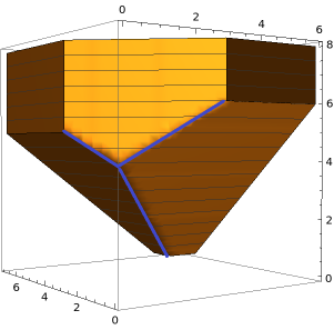
(b) 3-point

Figure 1: a) The yellow area is the set of all possible radius functions on $2$ points and the line segment colored in blue refers to the minimal ones.
b) The three dimensional polyhedron is the set of all possible radius functions on $3$ points and the tripod consisting of three line segments colored in blue refers to the minimal ones.

For the analysis of discrete metric spaces, some variants of the notion of hyperconvexity are well suited, c.f [33, 20, 23, 24].

Definition 4.2.

$(X,d)$ is $\delta$-hyperbolic ($\delta\geq 0$) if for any family $\{B(x_{i},r_{i})\}_{i\in I}$ with $r_{i}+r_{j}\geq d(x_{i},x_{j})$,

$$\bigcap_{i\in I}B(x_{i},\delta+r_{i})\neq\emptyset.$$ (9)

Definition 4.3.

$(X,d)$ is $\lambda$-hyperconvex ($\lambda\geq 1$) if for every family $\{B(x_{i},r_{i})\}_{i\in I}$ with $r_{i}+r_{j}\geq d(x_{i},x_{j})$,

$$\bigcap\limits_{i\in I}B(x_{i},\lambda r_{i})\neq\emptyset.$$ (10)

Of course, $0$-hyperbolicity and $1$-hyperconvexity are simply hyperconvexity. For large radii, $\delta$ insignificant, and the concept of $\delta$-hyperbolicity is therefore good for asymptotic considerations. In contrast, $\lambda$-hperconvexity is invariant under scaling the metric $d$, and it can therefore capture scaling invariant properties of a metric space.
The preceding concepts allow for a quantification of the deviation from hyperconvexity. The following results are known.

Theorem 4.2.

Hilbert spaces are $\sqrt{2}$-hyperconvex. Reflexive and dual Banach spaces are $2$-hyperconvex. Therefore, for a measure space $(X,\mu)$, $L^{p}(X,\mu),1<p<\infty$, are $2$-hyperconvex, and if $X$ is finite, $L^{1}(X,\mu)$ is also $2$-hyperconvex. $L^{\infty}(X,\mu)$ is hyperconvex. [33, 20]

5 Relation with Topological Data Analysis (TDA)

Definition 5.1.

For a family $(x_{i})_{i\in I}$ in a metric space $(X,d)$ and $r>0$, we define the Čech complex $\check{C}_{r}((x_{i}),X)$ containing a $q$-simplex whenever

$$\bigcap_{i=1,\dots,q+1}B(x_{i},r)\neq\emptyset.$$

Here $(x_{i})_{i\in I}$ is called the landmark set and $X$ is the witness set. When the witness set coincides with the landmarks, we thus define a non-empty intersection inside the sample set $(x_{i})_{i\in I}$ as the criterion for a simplex. We also define the Vietoris-Rips complex $VR_{r}((x_{i}),X)$ containing a $q$-simplex whenever

$$B(x_{i},r)\cap B(x_{j},r)\neq\emptyset\ \text{ for all }i,j\in I.$$

The two structures are not as different as they might appear, as the difference between the criteria for spanning a simplex is whether the vertex set is contained in a ball of radius or of diameter $r$.
The principle of the important topological data analysis scheme of persistent homology then is to record how the homology of these complexes varies as a function of $r$. [19, 42, 18, 12]
Of course, every simplex of the Čech complex is also a simplex of the Vietoris-Rips complex, but not necessarily conversely unless for each simplex at least one of the balls of diameter $r$ containing the vertex set of that simplex has a center in the witness set.
Deviation from hyperconvexity lets the Vietoris-Rips complex contain more simplices than the Čech complex, or conversely

Lemma 5.1.

In a hyperconvex space, all simplices that are filled in the Vietoris-Rips complex are also filled in the Čech complex. In particular, there is no contribution to local homology from unfilled simplices. ∎

For instance, we can take a sample $(x_{i})_{i\in I}$ from a geodesic metric space $(X,d)$ and compare $VR_{r}((x_{i}),X)$ with $\check{C}_{r}((x_{i}),E(X))$. For the latter complex, we take the hyperconvex hull of $X$, i.e. $E(X)$, as the witness set. It is clear that $\check{C}_{r}((x_{i}),E(X))\subset VR_{r}((x_{i}),X)$, as $X$ is a geodesic space and hence totally convex. Conversely, every simplex in $VR_{r}((x_{i}),X)$ is defined according to the criterion that balls of radius $r$ around its vertices intersect pairwise, which by hyperconvexity of $E(X)$ implies the existence of a common point between them in $E(X)$. In other words, the Vietoris-Rips complex of a metric family $(x_{i})_{i\in I},d$ coincides with its Čech complex but with different witness sets. This natural principle has been used in [36] to study the metric thickening of $S^{1}$ in its hyperconvex hull. A thorough study of the Čech and the Vietoris-Rips filtration of $S^{1}$ can be found in [2, 1].
If $X$ is a closed Riemannian manifold, for small-enough radius $r$ depending on the injectivity radius and a curvature bound, $VR_{r}(X)$ is homotopy equivalent to $X$ by a well known theorem of Hausmann [27]. On the other hand according to the nerve lemma, whenever $X$ is a paracompact space and the family of open balls around sample points $(x_{i})_{i\in I}$ with radius $r>0$ define a cover such that the non-empty intersections of any finite number of them is contractible, the Čech complex $\check{C}_{<r}((x_{i}),X)$ is homotopy equivalent to the original space $X$, c.f. [26]. Although Hausmann’s theorem is restricted to the case where the original space, from which the sample is taken, is a Riemannian manifold, both construction at some point reveal the topology of the space. However, the Vietoris-Rips filtration ignores the geometry of the space beyond the pairwise relations. The extent to which higher order relations are overlooked by considering Vietoris-Rips complexes can be quantified by computing the deviation from hyperconvexity of different orders. This measures how much one must expand balls to obtain a simplex in the Čech complex of $(x_{i})$ with witness set $X$ after that simplex is observed in the Čech complex of $(x_{i})$ with witness set $E(X)$. The upper bound $2$ for this scale is usually stated in the TDA literature, but this bound is not sharp.
For instance, let us consider equilateral triangles of perimeter $3a$ in the Euclidean plane, in a circle and in a metric tree. That is, $(x_{1},x_{2},x_{3})$, $(x^{\prime}_{1},x^{\prime}_{2},x^{\prime}_{3})$ and $(\bar{x}_{1},\bar{x}_{2},\bar{x}_{3})$ are comparison triangles in the Euclidean plane, a circle and a hyperconvex space, respectively. As noted in (3), $r=\frac{a}{2}$ is the radius at which each of these triples forms a simplex in the corresponding Vietoris-Rips complex. However, we only need the upper bound of $2$ in the case of $(x^{\prime}_{1},x^{\prime}_{2},x^{\prime}_{3})$, where the point are sampled from a circle which has the highest deviation from hyperconvexity, for expanding the balls to obtain the simplex in the Čech complex, c.f. [31].
One can also more generally let the radii of the balls be different. That is, for a vertex set $(x_{i})_{i\in I}$ and a corresponding non-negative radius function $r$, we define the Čech complex containing a $q$-simplex $x_{1},...,x_{q+1}$ whenever

$$\bigcap_{i=1,\dots,q+1}B(x_{i},r(x_{i}))\neq\emptyset.$$

The Vietoris-Rips complex is defined in a similar way. And one can then look at the resulting constructions for all such radius functions simultaneously [31].

6 Curvature

We can use the preceding concepts to compare spaces with each other, or with reference spaces, like Euclidean space. In geometry, such a comparison is quantified by the concept of curvature. From our abstract perspective, curvature relates intersection patterns of balls to convexity properties of distance functions.

As pointed out by Klingenberg [34], the beginning of the theory of spaces of negative curvature can be dated to the work of von Mangoldt [41] in 1881 who showed that on a complete simply connected surface of negative curvature, geodesics starting at the same point diverge and can never meet again. This implies that the exponential map is a diffeomorphism. Apparently unaware of von Mangoldt’s work, Hadamard [25] in 1898 proved further results about geodesics on surfaces of negative curvature. E.Cartan [13] later considered negatively curved Riemannian manifolds of any dimension. For our purposes, non-positive, as opposed to negative, curvature is the appropriate concept, as we are interested in comparison theorems.

Let us first recall a by now classical concept of non-positive curvature, introduced by Alexandrov [4].

Definition 6.1.

The geodesic space $(X,d)$ is a $CAT(0)$-space if for all geodesics $c_{1},c_{2}:[0,1]\longrightarrow X$ with $c_{1}(0)=c_{2}(0)$

$$d(c_{1}(t),c_{2}(s))\leq\|{\bar{c}_{1}(t)-\bar{c}_{2}(s)}\|,\,\forall\ t,s\in[0,1]$$ (11)

where $\bar{c}_{1},\bar{c}_{2}:[0,1]\longrightarrow\mathbb{R}^{2}$ are the sides of the Euclidean comparison triangle in $\mathbb{R}^{2}$ with the same side lengths as the triangle $\bigtriangleup(c_{1}(0),c_{1}(1),c_{2}(1))$.

According to this definition, triangles in $CAT(0)$-spaces are not thicker than Euclidean triangles with the same side lengths, c.f. [32, 10, 9, 3]

There is another important concept of non-positive curvature, introduced by Busemann [11].

Definition 6.2.

A geodesic space $(X,d)$ is a Busemann convex space if for every two geodesics $c_{1},c_{2}:[0,1]\longrightarrow X$ with $c_{1}(0)=c_{2}(0)$, the distance function $t\mapsto d(c_{1}(t),c_{2}(t))$ is convex.

Geodesics in Busemann space diverge at least as fast as in Euclidean space.
Every $CAT(0)$ space is Busemann convex but not conversely. For complete Riemannian manifolds, however, the two definitions agree and are equivalent to non-positive sectional curvature in the sense of Riemann.
Several generalizations of these definitions to metric spaces that are not necessarily geodesic have been proposed, for instance [7, 8, 3]. We now present our definition from [30].

Definition 6.3.

The metric space $(X,d)$ has non-positive curvature if for each triple $(x_{1},x_{2},x_{3})$ in $X$ with the comparison triangle $\bigtriangleup(\bar{x}_{1},\bar{x}_{2},\bar{x}_{3})$ in ${\mathbb{R}}^{2}$, one has

$$\rho(x_{1},x_{2},x_{3})\leq\rho(\bar{x}_{1},\bar{x}_{2},\bar{x}_{3}),$$

where $\rho(\bar{x}_{1},\bar{x}_{2},\bar{x}_{3})$ is similarly defined by

$$\rho(\bar{x}_{1},\bar{x}_{2},\bar{x}_{3}):=\min_{x\in{\mathbb{R}}^{2}}\max_{i=1,2,3}\dfrac{\|x-\bar{x}_{i}\|}{r_{i}}.$$

According to this definition, the circumcenter of a triangle in a non-positively curved space is at least as close to the vertices as in the Euclidean case. In other words, there is chance of finding a better intermediate point for each triple of points in such a space than in Euclidean plane.
For any triple of closed balls $\{B(x_{i},r_{i});\>i=1,2,3\}$ with pairwise intersection, $\bigcap_{i=1,2,3}B(x_{i},\rho r_{i})$ is non-empty whenever $B(\bar{x}_{i},\rho r_{i})$, $i=1,2,3$, have a common point. Thus, balls do not need to be enlarged more than in Euclidean case to get triple intersection. Thus, we can again formulate a

Principle 6.1.

Balls intersect at least as easily as in Euclidean space.

Examples:

• Tripod spaces have non-positive curvature in the sense of Def. 6.3, because there, $\rho=1$, which is the smallest possible value.

• Complete $CAT(0)$ spaces have non-positive curvature in the sense of Def. 6.3. The converse not true; in fact, our spaces need not be geodesic, nor have unique geodesics.

• Approximate version applies to discrete spaces. This is obviously important for questions of data analysis, and this in fact constitutes one of the motivations for Def. 6.3.

We also have

Theorem 6.1.

A complete Riemannian manifold $(N,g)$ has non-positive curvature iff it has non-positive sectional curvature, c.f. [30].

Obviously, with the same concepts and constructions, one can also define upper curvature bounds other than 0, by comparison with suitably scaled 2-spheres or hyperbolic planes.

7 Conclusions

The Čech construction assigns to a cover $\mathcal{U}=(U_{i})_{i\in I}$ of $X$ a simplicial complex $\Sigma(\mathcal{U})$ with vertex set $I$ and a simplex $\sigma_{J}$ whenever $\bigcap_{j\in J}U_{j}\neq\emptyset$ for $J\subset I$.When all intersections are contractible, the homology of $\Sigma(\mathcal{U})$ equals that of $X$ (under some rather general topological conditions on $X$). When $(X,d)$ is metric space, we can use covers by (open or closed) distance balls. Now, when $(X,d)$ is a hyperconvex metric space, and if we use a cover $\mathcal{U}$ by distance balls, then whenever

$$\bigcap_{j\in J\backslash\{j_{0}\}}U_{j}\neq\emptyset\text{ for every }j_{0}\in J,$$ (12)

then also

$$\bigcap_{j\in J}U_{j}\neq\emptyset,$$ (13)

i.e., whenever $\Sigma(\mathcal{U})$ contains all the boundary facets of some simplex, it also contains that simplex itself. It even satisfies the stronger condition that whenever $\Sigma(\mathcal{U})$ contains all the boundary faces of dimension $1$ of some simplex, it also contains that simplex itself. This means that $\Sigma(\mathcal{U})$ is a flag complex. Thus, there are no holes of the type of unfilled simplices, and no corresponding contributions to homology groups.

As hyperconvex spaces are contractible, then whenever non-trivial homology groups arise in Čech filtrations, the space cannot be hyperconvex, but only $\lambda$-hyperconvex for some $\lambda>1$. But every complete metric space is $\lambda$-hyperconvex for some $1\leq\lambda\leq 2$, c.f. [24]. (In the discrete case, one might work also with $\delta$-hyperbolicity for $\delta>0$.)
From that perspective, hyperconvex spaces are the simplest model spaces, and homology can be seen as a topological measure for the deviation from such a model. However, this geometric interpretation has been dismissed in topological data analysis, by considering the Vietoris-Rips filtration instead of Čech, for the benefit of reducing computational complexity. Still, it is possible to infer topological information about a space from the Vietoris-Rips filtration, based on Hausmann’s theorem. However, when one samples a metric space, this depends on how dense sample is and the results are accurate only for small radii. For instance, the Vietoris-Rips complexes of $S^{1}$ admit holes of dimension larger than $1$ as the radius increases, c.f. [1].

Homology groups, and Betti numbers as integer invariants are fundamental topological invariants. Geometry can provide more refined real valued invariants. And after Riemann [38, 39], the fundamental geometric invariants are curvatures. In our framework, the essential geometric content of curvature can be extracted for general metric spaces. The basic class of model spaces for curvature is given by the tripod spaces, a special class containing hyperconvex spaces. From that perspective, the geometric content of curvature in the abstract setting considered here is the deviation from the tripod condition. Euclidean spaces only have a subsidiary role, based on a normalization of curvature that assigns the value $0$ to them.
Considering Euclidean spaces as model spaces is traditionally justified by the fact that spaces whose universal cover has synthetic curvature $\leq 0$ in the sense of Alexandrov are homotopically trivial in the sense that their higher homotopy groups vanish. In technical terms, they are $K(\pi,1)$ spaces, with $\pi$ standing for the first homotopy group. The perspective developed here, however, is a homological and not a homotopical one, and therefore, our natural comparison spaces are tripods. We have started their investigation in [30, 31]. A more systematic investigation of their properties should be of interest.
In order to get stronger topological properties, like those of hyperconvex spaces, which are homologically trivial, we might need conditions involving collections of more than three points.
In fact, according [37, Theorem 4.2], If $X$ is a tripod Banach space on which every collection of four closed balls $\{B(x_{i},r_{i})\}_{i=1}^{4}$ with non-empty pairwise intersection has a non-void intersection, then every finite family of closed balls with non-empty pairwise intersection has also a non-trivial intersection. In this case, the Vietoris-Rips and Čech complexes coincide.

One can also think about higher order relations and how they can be obtained from sub-relations (that is from the relations existing in all subsets of some smaller size). For instance, in some metric spaces, a family of $n$ balls has a common point if every subfamily of size $k$ in it has a non-empty intersection. [37] calls this property the $(n,k)$-intersection property. For instance, Helly’s theorem says that Euclidean space ${\mathbb{R}}^{d}$ has the $(n,d+1)$-intersection property for $n\geq d+2$. For a given metric space, one can compute the deviation from such a property.
From the perspective of Čech complexes, this deviation could be quantified by the scaling parameter needed to fill an $(n-1)$-simplex after all the faces of dimension $k-1$ are filled. The quantitative measure we introduced provides us with the scaling function to fill a $2$-simplex after its $1$-dimensional boundary faces are filled.

References

- [1] M. Adamaszek and H. Adams. The vietoris–rips complexes of a circle. Pacific Journal of Mathematics, 290(1):1–40, 2017.
- [2] M. Adamaszek, H. Adams, F. Frick, C. Peterson, and C. Previte-Johnson. Nerve complexes of circular arcs. Discrete & Computational Geometry, 56(2):251–273, 2016.
- [3] S. Alexander, V. Kapovitch, and A. Petrunin. Alexandrov geometry. arXiv:1903.08539v1, 2019.
- [4] A. D. Alexandrov. Über eine Verallgemeinerung der Riemannschen Geometrie. Schr. Forschungsinst. Math. Berlin, 1:33–84, 1957.
- [5] N. Aronszajn and P. Panitchpakdii. Extension of uniformly continuous transformations and hyperconvex metric spaces. Pacific J. Math., 6:405–439, 1956.
- [6] Hans-Jürgen Bandelt and Andreas WM Dress. A canonical decomposition theory for metrics on a finite set. Advances in mathematics, 92(1):47–105, 1992.
- [7] M. Bačak, B.B. Hua, J. Jost, M Kell, and A. Schikorra. A notion of nonpositive curvature for general metric spaces. Diff.Geom.Appl., 38:22–32, 2015.
- [8] I. D. Berg and I. G. Nikolaev. Characterization of aleksandrov spaces of curvature bounded above by means of the metric cauchy-schwarz inequality. Michigan Math. J., 67:289–332, 1993.
- [9] M.R. Bridson and A. Haefliger. Metric spaces of non-positive curvature, volume 319. Springer Science & Business Media, 2013.
- [10] D. Burago, Yu. Burago, and S. Ivanov. A course in metric geometry. AMS, 2001.
- [11] H. Busemann. Spaces with non-positive curvature. Acta Mathematica, 80(1):259–310, 1948.
- [12] G. Carlsson. Topology and data. Bull.AMS, 46:255–308, 2009.
- [13] É. Cartan. La géométrie des espaces de Riemann. Gauthier-Villars, 1925.
- [14] J. A. De Loera, B. Sturmfels, and R. Thomas. Gröbner bases and triangulations of the second hypersimplex. Combinatorica, 15(3):409–424, 1995.
- [15] M. Develin. Dimensions of tight spans. Annals of Combinatorics, 10(1):53–61, 2006.
- [16] A. Dress. Trees, tight extensions of metric spaces, and the cohomological dimension of certain groups: A note on combinatorial properties of metric spaces. Adv. Math., 53:321–402, 1984.
- [17] A. Dress, K. T. Huber, and V. Moulton. An explicit computation of the injective hull of certain finite metric spaces in terms of their associated buneman complex. Adv. Math., 168:1–28, 2002.
- [18] H. Edelsbrunner and J. Harer. Persistent homology – a survey. Contemporary mathematics, 453:257–282, 2008.
- [19] H. Edelsbrunner, D. Letscher, and A. Zomorodian. Topological persistence and simplification. Foundations of Computer Science, 2000. Proceedings. 41st Annual Symposium on. IEEE,.
- [20] R. Espínola and M. A. Khamsi. Introduction to Hyperconvex Spaces, pages 391–435. Springer Netherlands, Dordrecht, 2001.
- [21] M. Gromov. Structures métriques pour les variétés riemanniennes. Rédigé par J. Lafontaine and P. Pansu. Cedic-Nathan, Paris, 1980.
- [22] M. Gromov. Metric structures for Riemannian and non-Riemannian spaces. Birkhäuser, 1999.
- [23] B. Grünbaum. On some covering and intersection properties in minkowski spaces. Pacific J. Math., 27:487–494, 1959.
- [24] B. Grünbaum. Some applications of expansion constants. Pacific J. Math., 10(1):193–201, 1960.
- [25] J. Hadamard. Sur la forme des lignes géodésiques à l’infini et sur les géodésiques des surfaces réglées du second ordre. Bulletin de la Société Mathématique de France, 26:195–216, 1898.
- [26] A. Hatcher. Algebraic topology. Cambridge Univ.Press, 2001.
- [27] J. C. Hausmann et al. On the vietoris-rips complexes and a cohomology theory for metric spaces. Annals of Mathematics Studies, 138:175–188, 1995.
- [28] H. Hirai. Characterization of the distance between subtrees of a tree by the associated tight span. Annals of Combinatorics, 10(1):111–128, 2006.
- [29] J. R. Isbell. Six theorems about injective metric spaces. Commentarii mathematici Helvetici, 39:65–76, 1964.
- [30] P. Joharinad and J. Jost. Topology and curvature of metric spaces. Adv. Math., 106813:106813, 2019.
- [31] P. Joharinad and J. Jost. Topological representation of the geometry of metric spaces. arXiv preprint arXiv:2001.10262, 2020.
- [32] J. Jost. Nonpositive curvature: Geometric and analytic aspects. Birkhäuser, 1997.
- [33] M. A. Khamsi, H. Knaust, N. T. Nguyen, and M. D. O’Neill. -hyperconvexity in metric spaces. Nonlinear Anal., 43:21–31, 2000.
- [34] W. Klingenberg. Riemannian geometry. de Gruyter, 1982.
- [35] U. Lang. Injective hulls of certain discrete metric spaces and groups. Journal of Topology and Analysis, 5(3):297–331, 2013.
- [36] S. Lim, F. Mémoli, and O. B. Okutan. Vietoris-rips persistent homology, injective metric spaces, and the filling radius. 2021. https://arxiv.org/abs/2001.07588v3.
- [37] J. Lindenstrauss. On the extension property for compact operators. Bulletin of AMS, 68:484–487, 1962.
- [38] B. Riemann. Ueber die Hypothesen, welche der Geometrie zu Grunde liegen. Edited with a commentary by J.Jost, Klassische Texte der Wissenschaft, Springer, Berlin etc., 2013.
- [39] B. Riemann. On the hypotheses which lie at the bases of geometry. Translated by W.K.Clifford, edited with a commentary by J.Jost, Classic Texts in the Sciences, Birkhäuser, 2016.
- [40] B. Sturmfels and J. Yu. Classification of six-point metrics. arXiv preprint math/0403147, 2004.
- [41] H. von Mangoldt. Ueber diejenigen Punkte auf positiv gekrümmten Flächen, welche die Eigenschaft haben, dass die von ihnen ausgehenden geodätischen Linien nie aufhören, kürzeste Linien zu sein. Crelle’s Journal (J. Reine Angew. Math.), 91:23–52, 1881.
- [42] A. Zomorodian and G. Carlsson. Computing persistent homology. Discrete & Computational Geometry, 33(2):249–274, 2005.