LiDAR-based 4D Panoptic Segmentation
via Dynamic Shifting Network

Abstract

With the rapid advances of autonomous driving, it becomes critical to equip its sensing system with more holistic 3D perception. However, existing works focus on parsing either the objects (e.g. cars and pedestrians) or scenes (e.g. trees and buildings) from the LiDAR sensor. In this work, we address the task of LiDAR-based panoptic segmentation, which aims to parse both objects and scenes in a unified manner. As one of the first endeavors towards this new challenging task, we propose the Dynamic Shifting Network (DS-Net), which serves as an effective panoptic segmentation framework in the point cloud realm. In particular, DS-Net has three appealing properties: 1) Strong backbone design. DS-Net adopts the cylinder convolution that is specifically designed for LiDAR point clouds. The extracted features are shared by the semantic branch and the instance branch which operates in a bottom-up clustering style. 2) Dynamic Shifting for complex point distributions. We observe that commonly-used clustering algorithms like BFS or DBSCAN are incapable of handling complex autonomous driving scenes with non-uniform point cloud distributions and varying instance sizes. Thus, we present an efficient learnable clustering module, dynamic shifting, which adapts kernel functions on the fly for different instances. 3) Extension to 4D prediction. Furthermore, we extend DS-Net to 4D panoptic LiDAR segmentation by the temporally unified instance clustering on aligned LiDAR frames. To comprehensively evaluate the performance of LiDAR-based panoptic segmentation, we construct and curate benchmarks from two large-scale autonomous driving LiDAR datasets, SemanticKITTI and nuScenes. Extensive experiments demonstrate that our proposed DS-Net achieves superior accuracies over current state-of-the-art methods in both tasks. Notably, in the single frame version of the task, we outperform the SOTA method by 1.8% in terms of the PQ metric. In the 4D version of the task, we surpass 2nd place by 5.4% in terms of the LSTQ metric.

1 Introduction

Figure 1: As shown in (a), LiDAR-based panoptic segmentation requires instance-level segmentation for things classes and semantic-level segmentation for stuff classes. (b) shows the core operation of the proposed dynamic shifting where several shift candidates are weighted to obtain the optimal shift target for each regressed center.

Autonomous driving, one of the most promising applications of computer vision, has achieved rapid progress in recent years. Perception system, one of the most important modules in autonomous driving, has also attracted extensive studies in previous research works. Admittedly, the classic tasks of 3D object detection [1, 2, 3] and semantic segmentation [4, 5, 6] have developed relatively mature solutions that support real-world autonomous driving prototypes. However, there still exists a considerable gap between the existing works and the goal of holistic perception which is essential for the challenging autonomous driving scenes. In this work, we propose to close the gap by exploring the task of LiDAR-based panoptic segmentation, which requires full-spectrum point-level predictions.

Panoptic segmentation has been proposed in 2D detection [7] as a new vision task which unifies semantic and instance segmentation. Behley et al. [8] extend the task to LiDAR point clouds and propose the task of LiDAR-based panoptic segmentation. As shown in Fig. 1 (a), this task requires to predict point-level semantic labels for background (stuff) classes (e.g. road, building and vegetation), while instance segmentation needs to be performed for foreground (things) classes (e.g. car, person and cyclist).

Nevertheless, the complex point distributions of LiDAR data make it difficult to perform reliable panoptic segmentation. Most existing point cloud instance segmentation methods [9, 10] are mainly designed for dense and uniform indoor point clouds. Therefore, decent segmentation results can be achieved through the center regression and heuristic clustering algorithms. However, due to the non-uniform density of LiDAR point clouds and varying sizes of instances, the center regression fails to provide ideal point distributions for clustering. The regressed centers usually form noisy strip distributions that vary in density and sizes. As will be analyzed in Section 3.2, several heuristic clustering algorithms widely used in previous works cannot provide satisfactory clustering results for the regressed centers of LiDAR point clouds. To tackle the above mentioned technical challenges, we propose Dynamic Shifting Network (DS-Net) which is specifically designed for effective panoptic segmentation of LiDAR point clouds.

Firstly, we adopt a strong backbone design and provide a strong baseline for the new task. Inspired by [11], the cylinder convolution is used to efficiently extract grid-level features for each LiDAR frame in one pass which are further shared by the semantic and instance branches.

Secondly, we present a novel Dynamic Shifting Module designed to cluster on the regressed centers with complex distributions produced by the instance branch. As illustrated in Fig. 1 (b), the proposed dynamic shifting module shifts the regressed centers to the cluster centers. The shift targets $x_{i}$ are adaptively computed by weighting across several shift candidates $c_{ij}$ which are calculated through kernel functions $k_{j}$. The special design of the module makes the shift operation capable of dynamically adapting to the density or sizes of different instances and therefore shows superior performance on LiDAR point clouds. Further analysis also shows that the dynamic shifting module is robust and not sensitive to parameter settings.

Thirdly, the Consensus-driven Fusion Module is presented to unify the semantic and instance results to obtain panoptic segmentation results. The proposed consensus-driven fusion mainly solves the disagreement caused by the class-agnostic style of instance segmentation. The fusion module is highly efficient, thus brings negligible computation overhead.

With the single frame version of DS-Net established, we further extend it to the new task of 4D panoptic LiDAR segmentation, which is first introduced by [12]. The task not only requires panoptic segmentation for each frame, but also consistent things IDs across frames. In order to achieve that, we propose the temporally unified instance clustering on the aligned and overlapped consequent frames to achieve instance segmentation and instance association at the same time. Temporally consistent instance segmentation is further fused with the semantic segmentation to form the final 4D panoptic LiDAR segmentation results.

Extensive experiments on SemanticKITTI demonstrate the effectiveness of our proposed DS-Net. To further illustrate the generalizability of DS-Net, we customize a LiDAR-based panoptic segmentation dataset based on nuScenes. As one of the first works for this new task, we present several strong baseline results by combining the state-of-the-art semantic segmentation and detection methods. DS-Net outperforms all the state-of-the-art methods on both benchmarks (1st place on the public leaderboard of SemanticKITTI).

The main contributions are summarized below: 1) To our best knowledge, we present one of the first attempts to address the challenging task of LiDAR-based panoptic segmentation. 2) The proposed DS-Net effectively handles the complex distributions of LiDAR point clouds, and achieves state-of-the-art performance on SemanticKITTI and nuScenes. 3) We extend DS-Net to the novel task of 4D panoptic LiDAR segmentation and achieve state-of-the-art results on SemanticKITTI. 4) Extensive experiments are performed on large-scale datasets. We adapt existing methods to this new task for in-depth comparisons. Further statistical analyses are carried out to provide valuable observations.

2 Related Work

Single Frame Panoptic Segmentation. The challenging vision task of panoptic segmentation is firstly defined by [7] where semantic segmentation for stuff classes [13] and instance segmentation for things classes are evaluated under unified metrices. From the perspective of network architecture, most panoptic segmentation methods can be categorized into top-down style and bottom-up style. The top-down methods are mostly based on MaskRCNN [14] where the instances are firstly detected then segmented by predicting masks. Main innovations of this kinds of methods lie in the following two aspects. The first one [15, 16, 17, 18] is the backbone where semantic and instance information are extracted and shared. Panoptic FPN [15] and Seamless [16] manage to share MaskRCNN Feature Pyramid Network (FPN) between semantic and instance branches which yields a solid and strong baseline for the emerging task. The second aspect [15, 19, 20, 21] is the handling of disagreement between semantic and instance segmentation predictions and conflicts between multiple instance segmentation predictions. UPSNet [22] and Li et al. [23] try to unify things and stuff segmentation by introducing panoptic logits which can generate coherent panoptic segmentation results without any post processing.

The bottom-up approaches [24, 25, 26] typically perform semantic segmentation first, then perform pixel clustering based on the semantic predictions, which natually saves the trouble of conflict handling and would lead to lighter network design. Although top-down approaches tend to outperform bottom-up approaches due to the use of the powerful MaskRCNN, recent work of Panoptic-DeepLab [25] presents a bottom-up baseline that has comparable performance with top-down methods. For the simplicity of the network design, we choose to use bottom-up approach in the proposed DS-Net.

Video Panoptic Segmentation. With the development of single frame panoptic segmentation techniques, recent researches have extended the task to video inputs. [27] first formally defined the task and evaluation metrics for video panoptic segmentation, which requires the consistency of things IDs across frames. [27] constructs the method based on UPSNet [22]. Consequent two frames are fused using spatial-temporal attention. Finally, an object-level tracking is performed for consistent things IDs. [28], however, adopts a bottom-up backbone. Center regression is performed for two consequent frames with the centers predicted from the first frame, which would naturally produce consistent things IDs.

Point Cloud Semantic and Instance Segmentation. According to the data representations of point clouds, most point cloud semantic segmentation methods can be categorized to point-based and voxel-based methods. Based on PointNet-like backbones [29, 30, 31], KPConv [32], DGCNN [33], PointConv [34] and Randla-Net [35] can directly operate on unordered point clouds. However, due to space and time complexity, most point-based methods struggle on large-scale point clouds datasets e.g. ScanNet [36], S3DIS [37], and SemanticKITTI [38]. MinkowskiNet [39] utilizes the sparse convolutions to efficiently perform semantic segmentation on the voxelized large-scale point clouds. SqueezeSeg [5] views LiDAR point clouds as range images while PolarNet [6] and Cylinder3D [11, 40, 41] divide the LiDAR point clouds under the polar and cylindrical coordinate systems.

Previous works have shown great progress in the instance segmentation of indoor point clouds. A large number of point-based methods (e.g. SGPN [42], ASIS [43], JSIS3D [44] and JSNet [45]) split the whole scene into small blocks and learn point-wise embeddings for final clustering, which are limited by the heuristic post processing steps and the lack of perception. To avoid the problems, recent works (e.g. PointGroup [10], 3D-MPA [9], OccuSeg [46]) use sparse convolutions to extract features of the whole scene in one pass. As for LiDAR point clouds, there are a few previous works [35, 47, 5, 48] trying to tackle the problem.

Point Cloud Panoptic Segmentation. Recently, several attempts [8, 49, 50, 51] have been made in the emerging task of point cloud panoptic segmentation. [8] first formally defines the task of LiDAR-based panoptic segmentation and proposes to combine the semantic segmentation and 3D object detection to obtain the panoptic segmentation results. [49] performs spherical projection on LiDAR point clouds and utilize a bottom-up 2D panoptic segmentation. [50] utilizes the Polar BEV encoder [6] to extract per-point features. A semantic segmentation and class-agnostic instance clustering technique is then used to obtain final results. [12] extend the single frame version of LiDAR-based panoptic segmentation to the 4D version by greedy cross-volume association based on the overlap score. Our proposed 4D panoptic LiDAR segmentation methods performs unified instance clustering on the overlapping consequent LiDAR scans to obtain consistent things IDs.

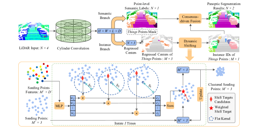
Figure 2: Architecture of the DS-Net. The DS-Net consists of the cylinder convolution, a semantic and an instance branch as shown in the upper part of the figure. The regressed centers provided by the instance branch are clustered by the novel dynamic shifting module which is shown in the bottom half. The consensus-driven fusion module unifies the semantic and instance results into the final panoptic segmentation results.

3 Our Approach

As one of the first attempts on the task of LiDAR-based panoptic segmentation, we first introduce a strong backbone to establish a simple baseline (Sec. 3.1), based on which two modules are further proposed. The novel dynamic shifting module is presented to tackle the challenge of the non-uniform LiDAR point clouds distributions (Sec. 3.2). The efficient consensus-driven fusion module combines the semantic and instance predictions and produces panoptic segmentation results (Sec. 3.3). The whole pipeline of the DS-Net is illustrated in Fig. 2. Finally, we introduce a simple yet effective extension to the task of 4D panoptic LiDAR segmentation. (Sec. 3.4)

3.1 Strong Backbone Design

To obtain panoptic segmentation results, it is natural to solve two sub-tasks separately, which are semantic and instance segmentation, and combine the results. As shown in the upper part of Fig. 2, the strong backbone consists of three parts: the cylinder convolution, a semantic branch, and an instance branch. High quality grid-level features are extracted by the cylinder convolution from raw LiDAR point clouds and then shared by semantic and instance branches.

Cylinder Convolution. Considering the difficulty presented by the task, we find that the cylinder convolution [11] best meets the strict requirements of high efficiency, high performance and fully mining of 3D positional relationship. The cylindrical voxel partition can produce more even point distribution than normal Cartesian voxel partition and therefore leads to higher feature extraction efficiency and higher performance. Cylindrical voxel representation combined with sparse convolutions can naturally retain and fully explore 3D positional relationship. Thus we choose the cylinder convolution as our feature extractor.

Semantic Branch. The semantic branch performs semantic segmentation by connecting MLP to the cylinder convolution to predict semantic confidences for each voxel grid. Specifically, the input LiDAR point clouds $P=\{p_{i}\}\in\mathbb{R}^{N\times 4}$, where $i\in\{1,...,N\}$, consists of $N$ points and each point has four attributes $p_{i}=(x_{i},y_{i},z_{i},r_{i})$ representing its XYZ coordinates and the intensity of the corresponding reflection beams. The output of the backbone is the voxel features $F_{v}\in\mathbb{R}^{H\times W\times L\times D}$, where $C$ represents the dimension of the features. As for semantic segmentation branch, by applying convolution to $F_{v}$, semantic logits $L_{s}\in\mathbb{R}^{H\times W\times L\times C}$, where $C$ is the number of all classes, are predicted for each voxel, which is then followed by max operation to compute the predicted semantic label for each voxel. Point-level semantic predictions are obtained by copying voxel labels to the points inside the voxels. Considering the category imbalance in autonomous driving scene, we choose Weighted Cross Entropy and Lovasz Loss as the loss function for semantic segmentation branch.

Instance Branch. The instance branch utilizes center regression to prepare the things points for further clustering. The center regression module uses MLP to adapt cylinder convolution features and make things points to regress the centers of their instances by predicting the offset vectors $O\in\mathbb{R}^{M\times 3}$ pointing from the points $P\in\mathbb{R}^{M\times 3}$ to the instance centers $C_{gt}\in\mathbb{R}^{M\times 3}$. The loss function for instance branch can be formulated as:

$$L_{ins}=\frac{1}{M}\sum_{i=0}^{M}\lVert O[i]-(C_{gt}[i]-P[i])\rVert_{1}\text{,}$$ (1)

where $M$ is the number of things points. The regressed centers $O+P$ are further clustered to obtain the instance IDs, which can be achieved by either heuristic clustering algorithms or the proposed dynamic shifting module which are further introduced and analyzed in the following section.

3.2 Dynamic Shifting

Point Clustering Revisit. Unlike indoor point clouds which are carefully reconstructed using RGB-D videos, the LiDAR point clouds have the distributions that are not suitable for normal clustering solutions used by indoor instance segmentation methods. The varying instance sizes, the sparsity and incompleteness of LiDAR point clouds make it difficult for the center regression module to predict the precise center location and would result in noisy long strips distribution as displayed in Fig. 1 (b) instead of an ideal ball-shaped cluster around the center. Moreover, as presented in Fig. 3 (a), the clusters formed by regressed centers that are far from the LiDAR sensor have much lower densities than those of nearby clusters due to the non-consistent sparsity of LiDAR point clouds. Facing the non-uniform distribution of regressed centers, heuristic clustering algorithms struggle to produce satisfactory results. Four major heuristic clustering algorithms that are used in previous bottom-up indoor point clouds instance segmentation methods are analyzed below.

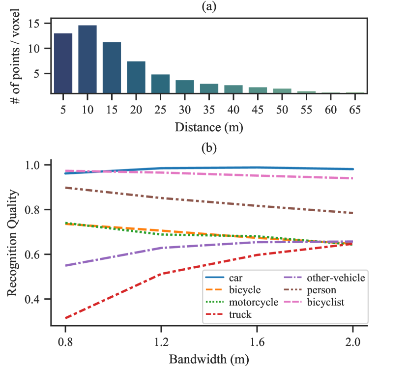
Figure 3: (a) counts the average number of regressed centers inside each valid voxel of instances at different distances. (b) shows the effect of Different Mean Shift Bandwidth on the Recognition Quality of Different Classes.

• Breadth First Search (BFS). BFS is simple and good enough for indoor point clouds as proved in [10], but not suitable for LiDAR point clouds. As discussed above, large density difference between clusters means that the fixed radius cannot properly adapt to different clusters. Small radius will over-segment distant instances while large radius will under-segment near instances.

• DBSCAN [52] and HDBSCAN [53]. As density-based clustering algorithms, there is no surprise that these two algorithms also perform badly on the LiDAR point clouds, even though they are proved to be effective for clustering indoor point clouds [9, 54]. The core operation of DBSCAN is the same as that of BFS. While HDBSCAN intuitively assumes that the points with lower density are more likely to be noise points which is not the case in LiDAR points.

• Mean Shift [55]. The advantage of Mean Shift, which is used by [56] to cluster indoor point clouds, is that the kernel function is not sensitive to density changes and robust to noise points which makes it more suitable than density-based algorithms. However, the bandwidth of the kernel function has great impact on the clustering results as shown in Fig. 3 (b). The fixed bandwidth cannot handle the situation of large and small instances simultaneously which makes Mean Shift also not the ideal choice for this task.

Figure 4: Architecture of the 4D version DS-Net (namely 4D-DS-Net). The 4D-DS-Net takes the aligned and overlapped LiDAR scans as input. Then perform unified instance clustering to generate temporally consistent things IDs. Finally the overlapped panoptic segmentation results are separated according to the original temporal masks.

Input: Things Points $P\in\mathbb{R}^{M\times 3}$, Things Features $F\in\mathbb{R}^{M\times D^{\prime}}$, Things Regressed Centers $C\in\mathbb{R}^{M\times 3}$, Fixed number of iteration $I\in\mathbb{N}$, Bandwidth candidates list $L\in\mathbb{R}^{l}$

Output: Instance IDs of things points $R\in\mathbb{R}^{M\times 1}$

1 $mask=FPS(P)$, $P^{\prime}=P[mask]$

2 $X=C[mask]$, $F^{\prime}=F[mask]$

3 for $i\leftarrow 1\ \textnormal{{to}}\ I$ do

4       $W_{i}=Softmax(MLP(F^{\prime}))$

5       $acc=zeros\_like(X)$

6       for $j\leftarrow 1\ \textnormal{{to}}\ l$ do

7             $K_{ij}=(XX^{T}\leq L[j])$

8             $D_{ij}=diag(K_{ij}\mathbf{1})$

9             $acc=acc+W_{i}[:,j]\odot(D_{ij}^{-1}K_{ij}X)$

10       end for

11      $X=acc$

12      

13 end for

14 $R^{\prime}=cluster(X)$

15 $index=nearest\_neighbour(P,P^{\prime})$

16 $R=R^{\prime}[index]$

return $R$

Algorithm 1 Forward Pass of the Dynamic Shifting Module

Dynamic Shifting. As discussed above, it is a robust way of estimating cluster centers of regressed centers by iteratively applying kernel functions as in Mean Shift. However, the fixed bandwidth of kernel functions fails to adapt to varying instance sizes. Therefore, we propose the dynamic shifting module which can automatically adapt the kernel function for each LiDAR point in the complex autonomous driving scene so that the regressed centers can be dynamically, efficiently and precisely shifted to the correct cluster centers.

In order to make the kernel function learnable, we first consider how to mathematically define a differentiable shift opration. Inspired by [57], the shift operation on the seeding points (i.e. points to be clustered) can be expressed as matrix operations if the number of iterations is fixed. Specifically, one iteration of shift operation can be formulated as follows. Denoting $X\in\mathbb{R}^{M\times 3}$ as the $M$ seeding points, $X$ will be updated once by the shift vector $S\in\mathbb{R}^{M\times 3}$ which is formulated as

$$X\leftarrow X+\eta S\text{,}$$ (2)

where $\eta$ is a scaling factor which is set to $1$ in our experiments.

The calculation of the shift vector $S$ is by applying kernel function $f$ on $X$, and formally defined as $S=f(X)-X$.

Among various kinds of kernel functions, the flat kernel is simple but effective for generating shift target estimations for LiDAR points, which is introduced as follows. The process of applying flat kernel can be thought of as placing a query ball of certain radius (i.e. bandwidth) centered at each seeding point and the result of the flat kernel is the mass of the points inside the query ball. Mathematically, the flat kernel $f(X)=D^{-1}KX$ is defined by the kernel matrix $K=(XX^{T}\leq\delta)$, which masks out the points within a certain bandwidth $\delta$ for each seeding point, and the diagonal matrix $D=diag(K\mathbf{1})$ that represents the number of points within the seeding point’s bandwidth.

With a differentiable version of the shift operation defined, we proceed to our goal of dynamic shifting by adapting the kernel function for each point. In order to make the kernel function adaptable for instances with different sizes, the optimal bandwidth for each seeding point has to be inferenced dynamically. A natural solution is to directly regress bandwidth for each seeding point, which however is not differentiable if used with the flat kernel. Even though Gaussian kernel can make direct bandwidth regression trainable, it is still not the best solution as analyzed in section 4.1. Therefore, we apply the design of weighting across several bandwidth candidates to dynamically adapt to the optimal one.

One iteration of dynamic shifting is formally defined as follows. As shown in the bottom half of Fig. 2, $l$ bandwidth candidates $L=\{\delta_{1},\delta_{2},...,\delta_{l}\}$ are set. For each seeding point, $l$ shift target candidates are calculated by $l$ flat kernels with corresponding bandwidth candidates. Seeding points then dynamically decide the final shift targets, which are ideally the closest to the cluster centers, by learning the weights $W\in\mathbb{R}^{M\times l}$ to weight on $l$ candidate targets. The weights $W$ are learned by applying MLP and Softmax on the backbone features so that $\sum_{j=1}^{l}W[:,j]=\textbf{1}$. The above procedure and the new learnable kernel function $\hat{f}$ can be formulated as

$$\hat{f}(X)=\sum_{j=1}^{l}W[:,j]\odot(D_{j}^{-1}K_{j}X)\text{,}$$ (3)

where $K_{j}=(XX^{T}\leq\delta_{j})$ and $D_{j}=diag(K_{j}\mathbf{1})$.

With the one iteration of dynamic shifting stated clearly, the full pipeline of the dynamic shifting module, which is formally defined in algorithm 1, can be illustrated as follows. Firstly, to maintain the efficiency of the algorithm, farthest point sampling (FPS) is performed on $M$ things points to provide $M^{\prime}$ seeding points for the dynamic shifting iterations (Lines 1–1). After a fixed number $I$ of dynamic shifting iterations (Lines 1–1), all seeding points have converged to the cluster centers. A simple heuristic clustering algorithm is performed to cluster the converged seeding points to obtain instance IDs for each seeding point (Line 1). Finally, all other things points find the nearest seeding points and the corresponding instance IDs are assigned to them (Lines 1–1).

The optimization of dynamic shifting module is not intuitive since it is impractical to obtain the ground truth bandwidth for each seeding point. The loss function has to encourage seeding points shifting towards their cluster centers which have no ground truths but can be approximated by the ground truth centers of instances $C_{gt}^{\prime}\in\mathbb{R}^{M^{\prime}\times 3}$. Therefore, the loss function for the $i$th iteration of dynamic shifting is defined by the manhattan distance between the ground truth centers $C_{gt}^{\prime}$ and the $i$th dynamically calculated shift targets $X_{i}$, which can be formulated as

$$l_{i}=\frac{1}{M^{\prime}}\sum_{x=1}^{M^{\prime}}\lVert X_{i}[x]-C_{gt}^{\prime}[x]\rVert_{1}\text{.}$$ (4)

Adding up all the losses of $I$ iterations gives us the loss function $L_{ds}$ for the dynamic shifting module: $L_{ds}=\sum_{i=1}^{I}w_{i}l_{i}\text{,}$ where $w_{i}$ are weights for losses of different iterations and are all set to $1$ in our experiments.

3.3 Consensus-driven Fusion

Typically, solving the conflict between semantic and instance predictions is one of the essential steps in panoptic segmentation. The advantages of bottom-up methods are that all points with predicted instance IDs must be in things classes and one point will not be assigned to two instances. The only conflict needs to be solved is the disagreement of semantic predictions inside one instance, which is brought in by the class-agnostic way of instance segmentation. The strategy used in the proposed consensus-driven fusion is majority voting. For each predicted instance, the most appeared semantic label of its points determines the semantic labels for all the points inside the instance. This simple fusion strategy is not only efficient but could also revise and unify semantic predictions using instance information.

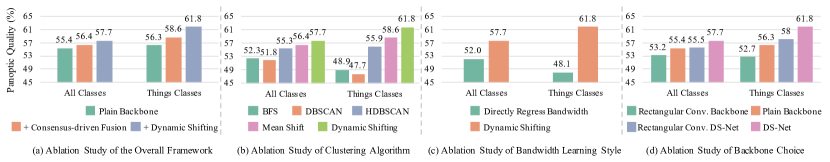
Figure 5: Ablation Study on the Validation Set of SemanticKITTI. The proposed two modules both contributes to the final performance of the DS-Net. The dynamic shifting module has advantages in clustering LiDAR point clouds. Weighting on bandwidth candidates is better than directly regressing bandwidth.

3.4 4D Panoptic LiDAR Segmentation

Based on the above proposed single version of the LiDAR-based panoptic segmentation method DS-Net, we further extend it to the task of 4D panoptic LiDAR segmentation.

To Extend from 3D to 4D. To extend from single frame panoptic segmentation to its 4D counterpart, the things IDs need to be consistent across frames. In other words, for the same instance observed in multiple frames, the target is to assign the same IDs for them. The trivial way is to append a tracking module to the instance segmentation branch to associate the predicted instance segments from previous and current frames. However, such naïve stacking of modules will inevitably lead to compromised performance of tracking due to its dependence on the segmentation quality. Moreover, the tracking module is hard to fully utilize the information provided by the consecutive LiDAR scans since it only processes the cropped partial observations. It is challenging for the tracking module to extract distinctive features from incomplete sparse point clouds. To fully utilize the temporal information from consecutive LiDAR scans, we propose to perform instance clustering in a temporally unified way, which is illustrated below.

Temporally Unified Instance Clustering. To ensure the consistency of the things IDs, we propose to use the temporally unified instance clustering to replace the explicit association. The target of such clustering strategy is to jointly cluster all the points of the same instance from several frames to a single cluster. Then we could naturally separate these points to different frames and allocate them the same instance ID. To fit such clustering strategy into the bottom-up pipeline, we need to modify the targets of the center regression step and the following clustering module. Assuming the point-level features of several consequent LiDAR frames are obtained, in the single frame version of the pipeline, the point-level features are used to regress the center of the instances. However, in the multi-frame scenario, the traffic participants like cars and pedestrians would move to different positions in different frames. Therefore, if we still follow the center regression target of the single frame version, there is great possibility of the same instance being clustered into multiple clusters because the regressed centers are too far apart due to high moving speed. To avoid such problem, for the same instance, we propose to regress to the center of the overlapped point clouds from multiple frames, which can be formulated as

$$C_{gt}(p_{id})=\text{center}(\{p|p\in gt_{t}(id)\ldots gt_{t+i}(id)\}),$$ (5)

where $p_{id}$ is the point that has the things ID of $id$, $gt_{t+i}(id)$ represents the set of points that have the things ID of $id$ and in frame $t+i$. After the adjusted center regression, the following clustering step is performed on the overlapped regressed centers. Unlike the 4D Volume Clustering proposed by [12], our clustering process does not take the frame timestamp of each point into consideration, which means our method is frame agnostic. Ideally, all the points of the same instance from several frames are clustered into a single cluster, which matches the target of the proposed temporally unified instance clustering. To integrate the clustering strategy into the single frame version DS-Net, we need to obtain the point-level features of several consequent LiDAR frames from the backbone. Features from different frames need to be aware of the information of each other. Otherwise, it is unreasonable to regress the centers of the overlapped point clouds. There are two possible ways to achieve that. The first one is to merge consequent LiDAR scans in the data level. The second one is to merge the feature map of each individual frame right after the backbone. From the perspective of computational efficiency, the first one is more efficient because only one 3D feature map need to be processed by the backbone. As for the performance, we find out that the first one is also a better strategy through extensive experiments. Therefore, based on the above analysis, we propose the 4D extension version of DS-Net, which is illustrated below.

4D extension of DS-Net. The 4D extension version of DS-Net (namely 4D-DS-Net) for the 4D panoptic segmentation is shown in Fig. 4. We first align consequent LiDAR point clouds and overlap them to get the temporally fused LiDAR point clouds. The fused LiDAR point clouds from frame $t$ to $t+i$ is defined as

$$P_{t:t+i} =\{p|p\in P_{t}^{\prime}\ldots P_{t+i}^{\prime}\}\text{, where}$$ (6)

$$P_{t+i}^{\prime} =((P_{t+i}R_{t+i}^{-1}+T_{t+i})-T_{t})R_{t},$$ (7)

$R_{t+i}$ and $T_{t+i}$ represent the rotation matrix and translation vector of frame $t+i$. The semantic segmentation branch predicts semantic labels for each point as that of the single version. The instance segmentation branch produces temporally consistent IDs for each point, which is achieved by the temporally unified instance clustering proposed above. Specifically, the foreground points are first regressed to the centers of the overlapped instances. Then, the regressed centers are further clustered by the proposed dynamic shifting network in the frame agnostic way. Such unified instance clustering step naturally associates the same instance across frames and saves the effort of tracking algorithms. Once we ensure the consistency of things IDs in two consequent frames, it is trivial to achieve such consistency across the whole sequences, which gives the final 4D panoptic segmentation results.

4 Experiments

TABLE I: LiDAR-based panoptic segmentation results on the validation set of SemanticKITTI. All results in [%].

Method	PQ	PQ$\dagger$	RQ	SQ	PQTh	RQTh	SQTh	PQSt	RQSt	SQSt	mIoU
KPConv [32] + PV-RCNN [2]	51.7	57.4	63.1	78.9	46.8	56.8	81.5	55.2	67.8	77.1	63.1
Cylinder3D [11] + PV-RCNN [2]	51.9	57.5	63.8	74.2	48.5	59.5	70.2	54.3	66.9	77.1	62.9
PointGroup [10]	46.1	54.0	56.6	74.6	47.7	55.9	73.8	45.0	57.1	75.1	55.7
LPASD [49]	36.5	46.1	-	-	-	28.2	-	-	-	-	50.7
PanosterK [58]	55.6	-	66.8	79.9	56.6	65.8	-	-	-	-	61.1
Panoptic-PolarNet [50]	59.1	64.1	70.2	78.3	65.7	74.7	87.4	54.3	66.9	71.6	64.5
DS-Net	57.7	63.4	68.0	77.6	61.8	68.8	78.2	54.8	67.3	77.1	63.5

TABLE II: LiDAR-based panoptic segmentation results on the test set of SemanticKITTI. All results in [%].

Method	PQ	PQ$\dagger$	RQ	SQ	PQTh	RQTh	SQTh	PQSt	RQSt	SQSt	mIoU
KPConv [32] + PointPillars [1]	44.5	52.5	54.4	80.0	32.7	38.7	81.5	53.1	65.9	79.0	58.8
RangeNet++ [4] + PointPillars [1]	37.1	45.9	47.0	75.9	20.2	25.2	75.2	49.3	62.8	76.5	52.4
KPConv [32] + PV-RCNN [2]	50.2	57.5	61.4	80.0	43.2	51.4	80.2	55.9	68.7	79.9	62.8
LPASD [49]	38.0	47.0	48.2	76.5	25.6	31.8	76.8	47.1	60.1	76.2	50.9
PanosterK [58]	52.7	59.9	64.1	80.7	49.4	58.5	83.3	55.1	68.2	78.8	59.9
4D-PLS [12]	50.3	57.8	61.0	81.6	-	-	-	-	-	-	61.3
Panoptic-PolarNet [50]	54.1	60.7	65.0	81.4	53.3	60.6	87.2	54.8	68.1	77.2	59.5
DS-Net	55.9	62.5	66.7	82.3	55.1	62.8	87.2	56.5	69.5	78.7	61.6

We conduct experiments on two large-scale datasets: SemanticKITTI [38] and nuScenes [59]. In addition, we evaluate our extension of 4D panoptic segmentation on SemanticKITTI.

SemanticKITTI. SemanticKITTI is the first dataset that presents the challenge of LiDAR-based panoptic segmentation and provides the benchmark[8]. SemanticKITTI contains 23,201 frames for training and 20,351 frames for testing. There are 28 annotated semantic classes which are remapped to 19 classes for the LiDAR-based panoptic segmentation task, among which 8 classes are things classes, and 11 classes are stuff classes. Each point is labeled with a semantic label and an temporally consistent instance ID which will be set to 0 if the point belongs to stuff classes.

nuScenes. In order to demonstrate the generalizability of DS-Net, we construct another LiDAR-based panoptic segmentation dataset from nuScenes. With the point-level semantic labels from the newly released nuScenes lidarseg challenge and the bounding boxes provided by the detection task, we could generate instance labels by assigning instance IDs to points inside bounding boxes. Following the definition of the nuScenes lidarseg challenge, we mark 10 foreground classes as things classes and 6 background classes as stuff classes out of all 16 semantic classes. The training and validation set has 28,130 and 6,019 frames.

Evaluation Metrics of LiDAR-based Panoptic Segmentation. As defined in [8], the evaluation metrics of LiDAR-based panoptic segmentation are the same as that of image panoptic segmentation defined in [7] including Panoptic Quality (PQ), Segmentation Quality (SQ) and Recognition Quality (RQ) which are calculated across all classes. For each class, the PQ, SQ and RQ are defined as

$$\text{PQ}=\underbrace{\frac{\sum_{(i,j)\in TP}\text{IoU}(i,j)}{|TP|}}_{\text{SQ}}\times\underbrace{\frac{|TP|}{|TP|+\frac{1}{2}|FP|+\frac{1}{2}|FN|}}_{\text{RQ}}.$$ (8)

The above three metrics are also calculated separately on things and stuff classes which give PQ^Th, SQ^Th, RQ^Th, and PQ^St, SQ^St, RQ^St. PQ^$\dagger$ is defined by swapping PQ of each stuff class to its IoU then averaging over all classes. In addition, mean IoU (mIoU) is also used to evaluate the quality of the sub-task of semantic segmentation.

Evaluation Metrics of 4D Panoptic LiDAR Segmentation. Several metrics are proposed by previous video panoptic segmentation works [27, 28, 12]. Among them, we choose to use LSTQ (LIDAR Segmentation and Tracking Quality) [12] as the evaluation metrics for 4D Panoptic Segmentation, which is defined as

$$\text{LSTQ}=\sqrt{\underbrace{\frac{1}{C}\sum_{c=1}^{C}\text{IoU}(c)}_{\text{S\textsubscript{cls}}}\times\underbrace{\frac{1}{T}\sum_{t\in T}\frac{\sum_{s\in S}\text{TPA}(s,t)\text{IoU}(s,t)}{|gt_{id}(t)|}}_{\text{S\textsubscript{assoc}}}},$$ (9)

where S_cls and S_assoc reflects the segmentation and tracking quality respectively. TPA (True Positive Association) is defined as $TPA(i,j)=|pr(i)\cap gt(j)|$, which represents the number of intersection between points that are predicted as $i$ and the ground truth points that have the id of $j$.

Implementation Details of Backbone. For both datasets, each input point is represented as a $4$ dimension vector including XYZ coordinates and the intensity. The backbone voxelizes a single frame to $480\times 360\times 32$ voxels under the cylindrical coordinate system. For that we should not use the information of bounding boxes in this segmentation task, the ground truth center of each instance is approximated by the center of its tight box that parallel to axes which makes a better approximation than the mass centers of the incomplete point clouds. The bandwidth of the Mean Shift used in our backbone method is set to $1.2$. Adam solver is utilized to optimize the network. The minimum number of points in a valid instance is set to 50 for SemanticKITTI and 5 for nuScenes.

Implementation Details of Dynamic Shifting. The number of the FPS downsampled points in the dynamic shifting module is set to $10000$. The final heuristic clustering algorithm used in the dynamic shifting module is Mean Shift with $0.65$ bandwidth for SemanticKITTI and BFS with $1.2$ radius for nuScenes. Bandwidth candidates are set to $0.2$, $1.7$ and $3.2$ for both datasets. The number of Iterations is set to $4$ for both datasets. We train the network with the learning rate of $0.002$, epoch of $50$ and batch size of $4$ on four Geforce GTX 1080Ti. The dynamic shifting module only takes 3-5 hours to train on top of a pretrained backbone.

Implementation Details of 4D-DS-Net. Two consequent LiDAR scans are aligned and overlapped for the training and inference of 4D panoptic segmentation. The number of the FPS downsampled points in the dynamic shifting module is set to $20000$. Other hyper-parameters are the same as its single version counterpart.

TABLE III: LiDAR-based panoptic segmentation results on the validation set of nuScenes. All results in [%].

Method	PQ	PQ$\dagger$	RQ	SQ	PQTh	RQTh	SQTh	PQSt	RQSt	SQSt	mIoU
Cylinder3D [11] + PointPillars [1]	36.0	44.5	43.0	83.3	23.3	27.0	83.7	57.2	69.6	82.7	52.3
Cylinder3D [11] + SECOND [3]	40.1	48.4	47.3	84.2	29.0	33.6	84.4	58.5	70.1	83.7	58.5
DS-Net	42.5	51.0	50.3	83.6	32.5	38.3	83.1	59.2	70.3	84.4	70.7

4.1 Ablation Study

Ablation on Overall Framework. To study on the effectiveness of the proposed modules, we sequentially add consensus-driven fusion module and dynamic shifting module to the bare backbone. The corresponding PQ and PQ^Th are reported in Fig. 5 (a) which shows that both modules contribute to the performance of DS-Net. The novel dynamic shifting module mainly boosts the performance of instance segmentation which are indicated by PQ^Th where the DS-Net outperforms the backbone (with fusion module) by 3.2% in validation split.

Ablation on Clustering Algorithms. In order to validate our previous analyses of clustering algorithms, we swap the dynamic shifting module for four other widely-used heuristic clustering algorithms: BFS, DBSCAN, HDBSCAN, and Mean Shift. The results are shown in Fig. 5 (b). Consistent with our analyses in Sec. 3.2, the density-based clustering algorithms (e.g. BFS, DBSCAN, HDBSCAN) perform badly in terms of PQ and PQ^Th while Mean Shift leads to the best results among the heuristic algorithms. Moreover, our dynamic shifting module shows the superiority over all four heuristic clustering algorithms.

Ablation on Bandwidth Learning Styles. In the dynamic shifting module, it is natural to directly regress bandwidth for each point as mentioned in Sec. 3.2. However, as shown in the Fig. 5 (c), direct regression is hard to optimize in this case because the learning target is not straightforward. It is difficult to determine the best bandwidth for each point, and therefore impractical to directly apply supervision on the regressed bandwidth. Therefore, it is easier for the network to choose from and combine several bandwidth candidates.

Ablation on Backbone Choice. To demonstrate that the dynamic shifting module can apply to different backbones, we report the performance of a rectangular convolution version of plain backbone and DS-Net Fig. 5 (d). An improvement of 2.3% in terms of PQ on both the rectangular convolution version and cylinder convolution version of the plain backbone is achieved on the validation set of SemanticKITTI, which shows the generalizability of the proposed dynamic shifting module.

4.2 Evaluation Comparisons on SemanticKITTI

Comparison Methods. Since its one of the first attempts on LiDAR-based panoptic segmentation, we provide several strong baseline results in order to validate the effectiveness of DS-Net. As proposed in [8], one good way of constructing strong baselines is to take the results from semantic segmentation methods and detection methods, and generate panoptic segmentation results by assigning instance IDs to all points inside predicted bounding boxes. [8] has provided the combinations of KPConv [32] + PointPillars [1], and RangeNet++ [4] + PointPillars [1]. To make the baseline stronger, we combine KPConv [32] with PV-RCNN [2] which is the state-of-the-art 3D detection method. In addition to the above baselines, we also adapt the state-of-the-art indoor instance segmentation method PointGroup [10] using the official released codes to experiment on SemanticKITTI. We also compare with recent LiDAR-based Panoptic Segmentation works: LPASD [49], PanosterK [58] and Panoptic-PolarNet [50].

Evaluation Results. Table I and II shows that the DS-Net outperforms most existing methods in both validation and test splits by a large margin. It is worth noting that PointGroup [10] performs poorly on the LiDAR point clouds which shows that indoor solutions are not suitable for challenging LiDAR point clouds. In test split, the DS-Net outperforms state-of-the-art method Panoptic-PolarNet [50] by 1.8% in both PQ and PQ^Th.

4.3 Evaluation Comparisons on nuScenes

Comparison Methods. Similarly, two strong semantic segmentation + detection baselines are provided for comparison on nuScenes. The semantic segmentation method is Cylinder3D [11] and the detection methods are SECOND [3] and PointPillars [1]. For fair comparison, the detection networks are trained using single frames on nuScenes. The point-wise semantic predictions and predicted bounding boxes are merged in the following steps. First all points inside each bounding box are assigned a unique instance IDs across the frame. Then to unify the semantic predictions inside each instance, we assign the class labels of bounding boxes predicted by the detection network to corresponding instances.

Evaluation Results. As shown in Table III, our DS-Net outperforms the best baseline method in most metrics. Especially, we surpass the best baseline method by 2.4% in PQ and 3.5% in PQ^Th. Unlike SemanticKITTI, nuScenes is featured as extremely sparse point clouds in single frames which adds even more difficulties to panoptic segmentation. The results validate the generalizability and the effectiveness of our DS-Net.

TABLE IV: 4D panoptic LiDAR segmentation results on the validation set of SemanticKITTI. All results in [%]. RN: RangeNet++ [4]; KP: KPConv [32]; PP: PointPillars [1]; MOT: Multi-Object Tracking [60]; SFP: Scene Flow based Propagation [61].

Method	LSTQ	Sassoc	Scls	IoUst	IoUth
RN + PP + MOT	43.8	36.3	52.8	60.5	42.2
KP + PP + MOT	46.3	37.6	57.0	64.2	54.1
RN + PP + SFP	43.4	35.7	52.8	60.5	42.2
KP + PP + SFP	46.0	37.1	57.0	64.2	54.1
4D-PLS [12]	62.8	65.1	60.5	65.4	61.3
DS-Net + Tracking	65.9	68.4	63.1	64.0	61.9
DS-Net + Feat. Fus.	67.8	72.1	63.7	64.2	63.1
4D-DS-Net	68.0	71.3	64.8	64.5	65.30

TABLE V: 4D panoptic LiDAR segmentation results on the test set of SemanticKITTI. All results in [%]. RN: RangeNet++ [4]; KP: KPConv [32]; PP: PointPillars [1]; MOT: Multi-Object Tracking [60]; SFP: Scene Flow based Propagation [61].

Method	LSTQ	Sassoc	Scls	IoUst	IoUth
RN + PP + MOT	35.5	24.1	52.4	64.5	35.8
KP + PP + MOT	38.0	25.9	55.9	66.9	47.7
RN + PP + SFP	34.9	23.3	52.4	64.5	35.8
KP + PP + SFP	38.5	26.6	55.9	66.9	47.7
4D-PLS [12]	56.9	56.4	57.4	66.9	51.6
4D-DS-Net	62.3	65.8	58.9	65.6	49.8

TABLE VI: Results of Single Frame PQ Evaluation of 4D-DS-Net on the validation set of SemanticKITTI.

Name	PQ	PQ$\dagger$	PQTh	PQSt	mIoU
DS-Net	57.7	63.4	61.8	54.8	63.5
DS-Net + Feat. Fus.	58.6	63.9	63.4	55.0	63.7
4D-DS-Net	59.5	64.5	64.4	55.9	64.8

4.4 4D Panoptic LiDAR Segmentation Results

Comparison Methods. Since the task is fairly new, we choose to compare with the first work [12] that proposes this task, denoted as 4D-PLS, and several ‘Semantic Segmentation + 3D Object Detection + Tracking’ assembled baseline methods. Besides, we also construct a baseline method ‘DS-Net + Tracking’ by appending a tracking module [27] to the instance segmentation branch. As discussed in Sec. 3.4, we also implement the feature map fusion on top of DS-Net, namely ‘DS-Net + Feat. Fus.’. Specifically, we perform a max pooling operation on the aligned 3D feature maps extracted from consecutive LiDAR frames by the backbone. Then the fused feature map is fed to semantic and instance branches. We refer to our proposed method as ‘4D-DS-Net’.

Evaluation Results. As shown in Table IV and V, our proposed method surpasses all baseline methods and the state-of-the-art method 4D-PLS [12] in terms of the main metric LSTQ in both validation and test sets. Moreover, improvements of 9.4% and 1.5% in respect of S_assoc and S_cls on the test set are achieved by DS-Net, which shows that both the tracking and segmentation performance contribute to the overall 5.4% improvement of LSTQ. The proposed ‘4D-DS-Net’ also surpasses ‘DS-Net + Tracking’ by 2.1% in terms of LSTQ on the validations set, which proves that simply stacking modules is hard to fully utilize the temporal information as mentioned in Sec. 3.4. Moreover, ‘4D-DS-Net’ surpasses ‘DS-Net + Feat. Fus.’ by a small margin of 0.2% in terms of LSTQ. However, the amount of memory and computation overhead of ‘DS-Net + Feat. Fus.’ compared to that of ‘4D-DS-Net’ still justifies our preference of data-level fusion.

4D Panoptic Segmentation Improves the Single Frame PQ Evaluation. We also evaluate the single frame metrics using the 4D version of DS-Net on the validation set of SemanticKITTI. As shown in Table VI, the 4D version of DS-Net surpasses the single frame DS-Net by 1.8% in terms of PQ. It shows that the temporal information can largely enrich the semantic information extracted by the backbone and therefore improves the overall performance. The improved single frame segmentation quality also explains the better performance in the task of 4D panoptic LiDAR segmentation. Moreover, ‘4D-DS-Net’ also outperforms ‘DS-Net + Feat. Fus.’ by 0.9% in terms of PQ, which shows the superiority of data-level fusion over simple feature-level fusion. Of course, more complex feature fusion could be designed and has the potential of outperforming data-level fusion. But with minimal memory and computation overhead, data-level fusion is the first choice here.

4.5 Further Analysis

Robust to Parameter Settings. As shown in Table VII, six sets of bandwidth candidates are set for independent training and the corresponding results are reported. The stable results show that DS-Net is robust to different parameter settings as long as the picked bandwidth candidates are comparable to the instance sizes. Unlike previous heuristic clustering algorithms that require massive parameter adjustment, DS-Net can automatically adjust to different instance sizes and point distributions and remains stable clustering quality.

TABLE VII: Results of different bandwidth candidates settings. All results in [%].

Bandwidth Candidates (m)	PQ	PQ$\dagger$	RQ	SQ	mIoU
0.2, 1.1, 2.0	57.4	63.0	67.7	77.4	63.7
0.2, 1.3, 2.4	57.5	63.1	67.7	77.6	63.5
0.2, 1.5, 2.8	57.6	63.2	67.8	77.6	63.7
0.2, 1.7, 3.2	57.7	63.4	68.0	77.6	63.5
0.2, 1.9, 3.6	57.7	63.3	67.9	77.6	63.4
0.2, 2.1, 4.0	57.4	63.1	67.7	77.5	63.3

Interpretable Learned Bandwidths. By averaging the bandwidth candidates weighted by the learned weights, the learned bandwidths for every points could be approximated. The average learned bandwidths of different classes are shown in Fig. 6. The average learned bandwidths are roughly proportional to the instance sizes of corresponding classes, which is consistent with the expectation that dynamic shifting can dynamically adjust to different instance sizes.

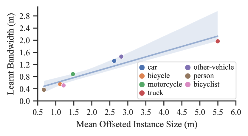
Figure 6: Proportional Relationship Between Sizes and the Learned Bandwidths. The $x$-axis represents the class-wise average size of regressed centers of instances while the $y$-axis stands for the average learned bandwidth of different things classes.

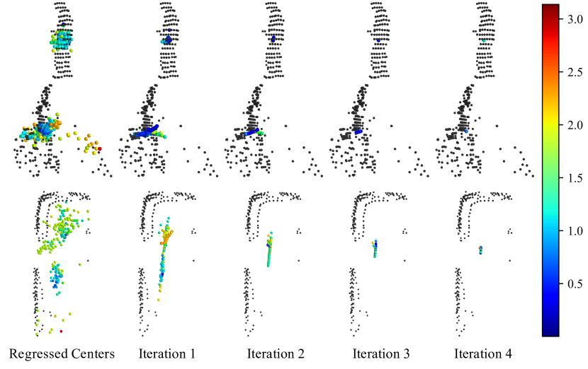
Figure 7: Visualization of Dynamic Shifting Iterations. The black points are the original LiDAR point clouds of instances. The colored points are seeding points. From left to right, with the iteration number increases, the seeding points converge to cluster centers.

Visualization of Dynamic Shifting Iterations. As visualized in Fig. 7, the black points are the original point clouds of different instances including person, bicyclist and car. The seeding points are colored in spectral colors where the redder points represents higher learned bandwidth and bluer points represents lower learned bandwidth. The seeding points farther away from the instance centers tend to learn higher bandwidths in order to quickly converge. While the well-learned regressed points tend to have lower bandwidths to maintain their positions. After four iterations, the seeding points have converged around the instance centers.

Learned Bandwidths of Different Iterations. The average learned bandwidths of different iterations are shown in Fig. 8. As expected, as the iteration rounds grow, points of the same instance gather tighter which usually require smaller bandwidths. After four iterations, learned bandwidths of most classes have dropped to 0.2, which is the lowest they can get, meaning that four iterations are enough for things points to converge to cluster centers, which further validates the conclusion made in the last paragraph.

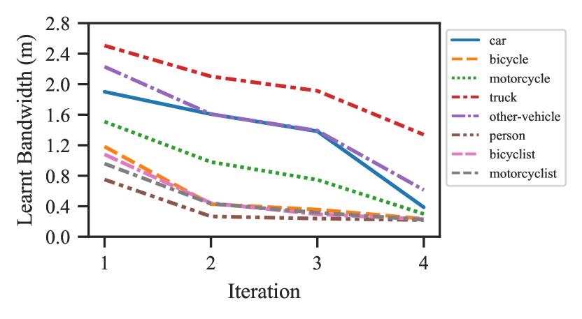
Figure 8: Relationship Between Iterations and the Learned Bandwidths. With number of iteration increases, the learned bandwidth decreases. At the 4th iteration, the learned bandwidths of most classes drop near the lower limit.

5 Conclusion

With the goal of providing holistic perception for autonomous driving, we are one of the first to address the task of LiDAR-based panoptic segmentation. In order to tackle the challenge brought by the non-uniform distributions of LiDAR point clouds, we propose the novel DS-Net which is specifically designed for effective panoptic segmentation of LiDAR point clouds. Our DS-Net adopts strong baseline design which provides strong support for the consensus-driven fusion module and the novel dynamic shifting module. The novel dynamic shifting module adaptively shifts regressed centers of instances with different density and varying sizes. The consensus-driven fusion efficiently unifies semantic and instance results into panoptic segmentation results. The DS-Net outperforms all strong baselines on both SemanticKITTI and nuScenes. Moreover, we extend the single version of DS-Net to the new task of LiDAR-based 4D panoptic segmentation and demonstrate state-of-the-art performance on SemanticKITTI. Further analyses show the robustness of the dynamic shifting module and the interpretability of the learned bandwidths.

Acknowledgments  This research was conducted in collaboration with SenseTime. This work is supported by NTU NAP and A*STAR through the Industry Alignment Fund - Industry Collaboration Projects Grant. This work is supported in part by Centre for Perceptual and Interactive Intelligence Limited, in part by the General Research Fund through the Research Grants Council of Hong Kong under Grants (Nos. 14208417 and 14207319), in part by CUHK Strategic Fund.

Fangzhou Hong received the BEng degree in Software Engineering from Tsinghua University, China, in 2020. He is currently a Ph.D. student in the School of Computer Science and Engineering at Nanyang Technological University. His research interests lie on the computer vision and deep learning. Particularly he is interested in 3D representation learning.

Hui Zhou received the bachelors and masters degree at university of science and electronic technology of china(UESTC) in 2015, 2018. He is currently a research scientist for autonomous driving in Sensetime Research. His research interests include computer vision and machine learning.

Xinge Zhu received the BEng degree in computer science from Shandong University, China, in 2015. He is working toward the PhD degree in The Chinese University of Hong Kong, under the supervision of Professor Dahua Lin. His research interests lie on the computer vision and machine learning. Particularly he is interested in 3D perception for autonomous vehicles, including 3D detection and 3D segmentation.

Hongsheng Li is an assistant professor in the Department of Electronic Engineering at the Chinese University of Hong Kong. In 2013-2015, he was an associate professor in the School of Electronic Engineering at University of Electronic Science and Technology of China. He received the bachelor’s degree in Automation from East China University of Science and Technology in 2006, and the doctorate degree in Computer Science from Lehigh University, United States in 2012. He has published over 70 papers in premier conferences on computer vision and machine learning, including CVPR, ICCV, ECCV, NeurIPS, ICLR, and AAAI. He received the 2020 IEEE CAS Society Outstanding Young Author Award. He won the first place in Object Detection from Videos (VID) track of ImageNet challenge 2016 as the team leader and 2015 as a team co-leader. He is an associate editor of Neurocomputing and serves as an area chair of NeurIPS 2021. His research interests include computer vision, machine learning, and medical image analysis.

Ziwei Liu is a Nanyang Assistant Professor at School of Computer Science and Engineering (SCSE) in Nanyang Technological University, with MMLab@NTU. Previously, he was a research fellow (2018-2020) in CUHK (with Prof. Dahua Lin) and a post-doc researcher (2017-2018) in UC Berkeley (with Prof. Stella X. Yu). His research interests include computer vision, machine learning and computer graphics. Ziwei received his Ph.D. (2013-2017) from CUHK / Multimedia Lab, advised by Prof. Xiaoou Tang and Prof. Xiaogang Wang. He is fortunate to have internships at Microsoft Research and Google Research. His works include Burst Denoising, CelebA, DeepFashion, Fashion Landmarks, DeepMRF, Voxel Flow, Long-Tailed Recognition, and Compound Domain Adaptation. His works have been transferred to products, including Microsoft Pix, SenseFocus, and Google Clips.

References

- [1] A. H. Lang, S. Vora, H. Caesar, L. Zhou, J. Yang, and O. Beijbom, “Pointpillars: Fast encoders for object detection from point clouds,” in Proceedings of the IEEE Conference on Computer Vision and Pattern Recognition, 2019, pp. 12 697–12 705.
- [2] S. Shi, C. Guo, L. Jiang, Z. Wang, J. Shi, X. Wang, and H. Li, “Pv-rcnn: Point-voxel feature set abstraction for 3d object detection,” in Proceedings of the IEEE/CVF Conference on Computer Vision and Pattern Recognition, 2020, pp. 10 529–10 538.
- [3] Y. Yan, Y. Mao, and B. Li, “Second: Sparsely embedded convolutional detection,” Sensors, vol. 18, no. 10, p. 3337, 2018.
- [4] A. Milioto, I. Vizzo, J. Behley, and C. Stachniss, “Rangenet++: Fast and accurate lidar semantic segmentation,” in 2019 IEEE/RSJ International Conference on Intelligent Robots and Systems (IROS). IEEE, 2019, pp. 4213–4220.
- [5] B. Wu, A. Wan, X. Yue, and K. Keutzer, “Squeezeseg: Convolutional neural nets with recurrent crf for real-time road-object segmentation from 3d lidar point cloud,” in 2018 IEEE International Conference on Robotics and Automation (ICRA). IEEE, 2018, pp. 1887–1893.
- [6] Y. Zhang, Z. Zhou, P. David, X. Yue, Z. Xi, B. Gong, and H. Foroosh, “Polarnet: An improved grid representation for online lidar point clouds semantic segmentation,” in Proceedings of the IEEE/CVF Conference on Computer Vision and Pattern Recognition, 2020, pp. 9601–9610.
- [7] A. Kirillov, K. He, R. Girshick, C. Rother, and P. Dollár, “Panoptic segmentation,” in Proceedings of the IEEE conference on computer vision and pattern recognition, 2019, pp. 9404–9413.
- [8] J. Behley, A. Milioto, and C. Stachniss, “A benchmark for lidar-based panoptic segmentation based on kitti,” arXiv preprint arXiv:2003.02371, 2020.
- [9] F. Engelmann, M. Bokeloh, A. Fathi, B. Leibe, and M. Nießner, “3d-mpa: Multi-proposal aggregation for 3d semantic instance segmentation,” in Proceedings of the IEEE/CVF Conference on Computer Vision and Pattern Recognition, 2020, pp. 9031–9040.
- [10] L. Jiang, H. Zhao, S. Shi, S. Liu, C.-W. Fu, and J. Jia, “Pointgroup: Dual-set point grouping for 3d instance segmentation,” in Proceedings of the IEEE/CVF Conference on Computer Vision and Pattern Recognition, 2020, pp. 4867–4876.
- [11] X. Zhu, H. Zhou, T. Wang, F. Hong, Y. Ma, W. Li, H. Li, and D. Lin, “Cylindrical and asymmetrical 3d convolution networks for lidar segmentation,” ArXiv, vol. abs/2011.10033, 2020.
- [12] M. Aygun, A. Osep, M. Weber, M. Maximov, C. Stachniss, J. Behley, and L. Leal-Taixé, “4d panoptic lidar segmentation,” in Proceedings of the IEEE/CVF Conference on Computer Vision and Pattern Recognition, 2021, pp. 5527–5537.
- [13] Z. Liu, X. Li, P. Luo, C.-C. Loy, and X. Tang, “Semantic image segmentation via deep parsing network,” in Proceedings of the IEEE international conference on computer vision, 2015, pp. 1377–1385.
- [14] K. He, G. Gkioxari, P. Dollár, and R. Girshick, “Mask r-cnn,” in Proceedings of the IEEE international conference on computer vision, 2017, pp. 2961–2969.
- [15] A. Kirillov, R. Girshick, K. He, and P. Dollár, “Panoptic feature pyramid networks,” in Proceedings of the IEEE Conference on Computer Vision and Pattern Recognition, 2019, pp. 6399–6408.
- [16] L. Porzi, S. R. Bulo, A. Colovic, and P. Kontschieder, “Seamless scene segmentation,” in Proceedings of the IEEE Conference on Computer Vision and Pattern Recognition, 2019, pp. 8277–8286.
- [17] Y. Li, X. Chen, Z. Zhu, L. Xie, G. Huang, D. Du, and X. Wang, “Attention-guided unified network for panoptic segmentation,” in Proceedings of the IEEE Conference on Computer Vision and Pattern Recognition, 2019, pp. 7026–7035.
- [18] Y. Wu, G. Zhang, Y. Gao, X. Deng, K. Gong, X. Liang, and L. Lin, “Bidirectional graph reasoning network for panoptic segmentation,” in Proceedings of the IEEE/CVF Conference on Computer Vision and Pattern Recognition, 2020, pp. 9080–9089.
- [19] H. Liu, C. Peng, C. Yu, J. Wang, X. Liu, G. Yu, and W. Jiang, “An end-to-end network for panoptic segmentation,” in Proceedings of the IEEE Conference on Computer Vision and Pattern Recognition, 2019, pp. 6172–6181.
- [20] Y. Yang, H. Li, X. Li, Q. Zhao, J. Wu, and Z. Lin, “Sognet: Scene overlap graph network for panoptic segmentation,” arXiv preprint arXiv:1911.07527, 2019.
- [21] Y. Chen, G. Lin, S. Li, O. Bourahla, Y. Wu, F. Wang, J. Feng, M. Xu, and X. Li, “Banet: Bidirectional aggregation network with occlusion handling for panoptic segmentation,” in Proceedings of the IEEE/CVF Conference on Computer Vision and Pattern Recognition, 2020, pp. 3793–3802.
- [22] Y. Xiong, R. Liao, H. Zhao, R. Hu, M. Bai, E. Yumer, and R. Urtasun, “Upsnet: A unified panoptic segmentation network,” in Proceedings of the IEEE Conference on Computer Vision and Pattern Recognition, 2019, pp. 8818–8826.
- [23] Q. Li, X. Qi, and P. H. Torr, “Unifying training and inference for panoptic segmentation,” in Proceedings of the IEEE/CVF Conference on Computer Vision and Pattern Recognition, 2020, pp. 13 320–13 328.
- [24] H. Wang, R. Luo, M. Maire, and G. Shakhnarovich, “Pixel consensus voting for panoptic segmentation,” in Proceedings of the IEEE/CVF Conference on Computer Vision and Pattern Recognition, 2020, pp. 9464–9473.
- [25] B. Cheng, M. D. Collins, Y. Zhu, T. Liu, T. S. Huang, H. Adam, and L.-C. Chen, “Panoptic-deeplab: A simple, strong, and fast baseline for bottom-up panoptic segmentation,” in Proceedings of the IEEE/CVF Conference on Computer Vision and Pattern Recognition, 2020, pp. 12 475–12 485.
- [26] H. Wang, Y. Zhu, B. Green, H. Adam, A. Yuille, and L.-C. Chen, “Axial-deeplab: Stand-alone axial-attention for panoptic segmentation,” arXiv preprint arXiv:2003.07853, 2020.
- [27] D. Kim, S. Woo, J.-Y. Lee, and I. S. Kweon, “Video panoptic segmentation,” in Proceedings of the IEEE/CVF Conference on Computer Vision and Pattern Recognition, 2020, pp. 9859–9868.
- [28] S. Qiao, Y. Zhu, H. Adam, A. Yuille, and L.-C. Chen, “Vip-deeplab: Learning visual perception with depth-aware video panoptic segmentation,” in Proceedings of the IEEE/CVF Conference on Computer Vision and Pattern Recognition, 2021, pp. 3997–4008.
- [29] C. R. Qi, H. Su, K. Mo, and L. J. Guibas, “Pointnet: Deep learning on point sets for 3d classification and segmentation,” in Proceedings of the IEEE conference on computer vision and pattern recognition, 2017, pp. 652–660.
- [30] C. R. Qi, L. Yi, H. Su, and L. J. Guibas, “Pointnet++: Deep hierarchical feature learning on point sets in a metric space,” in Advances in neural information processing systems, 2017, pp. 5099–5108.
- [31] X. Liu, Z. Han, F. Hong, Y.-S. Liu, and M. Zwicker, “Lrc-net: Learning discriminative features on point clouds by encoding local region contexts,” Computer Aided Geometric Design, vol. 79, p. 101859, 2020.
- [32] H. Thomas, C. R. Qi, J.-E. Deschaud, B. Marcotegui, F. Goulette, and L. J. Guibas, “Kpconv: Flexible and deformable convolution for point clouds,” in Proceedings of the IEEE International Conference on Computer Vision, 2019, pp. 6411–6420.
- [33] Y. Wang, Y. Sun, Z. Liu, S. E. Sarma, M. M. Bronstein, and J. M. Solomon, “Dynamic graph cnn for learning on point clouds,” Acm Transactions On Graphics (tog), vol. 38, no. 5, pp. 1–12, 2019.
- [34] W. Wu, Z. Qi, and L. Fuxin, “Pointconv: Deep convolutional networks on 3d point clouds,” in Proceedings of the IEEE Conference on Computer Vision and Pattern Recognition, 2019, pp. 9621–9630.
- [35] Q. Hu, B. Yang, L. Xie, S. Rosa, Y. Guo, Z. Wang, N. Trigoni, and A. Markham, “Randla-net: Efficient semantic segmentation of large-scale point clouds,” in Proceedings of the IEEE/CVF Conference on Computer Vision and Pattern Recognition, 2020, pp. 11 108–11 117.
- [36] A. Dai, A. X. Chang, M. Savva, M. Halber, T. Funkhouser, and M. Nießner, “Scannet: Richly-annotated 3d reconstructions of indoor scenes,” in Proceedings of the IEEE Conference on Computer Vision and Pattern Recognition, 2017, pp. 5828–5839.
- [37] I. Armeni, O. Sener, A. R. Zamir, H. Jiang, I. Brilakis, M. Fischer, and S. Savarese, “3d semantic parsing of large-scale indoor spaces,” in Proceedings of the IEEE Conference on Computer Vision and Pattern Recognition, 2016, pp. 1534–1543.
- [38] J. Behley, M. Garbade, A. Milioto, J. Quenzel, S. Behnke, C. Stachniss, and J. Gall, “Semantickitti: A dataset for semantic scene understanding of lidar sequences,” in Proceedings of the IEEE International Conference on Computer Vision, 2019, pp. 9297–9307.
- [39] C. Choy, J. Gwak, and S. Savarese, “4d spatio-temporal convnets: Minkowski convolutional neural networks,” in Proceedings of the IEEE Conference on Computer Vision and Pattern Recognition, 2019, pp. 3075–3084.
- [40] X. Zhu, H. Zhou, T. Wang, F. Hong, Y. Ma, W. Li, H. Li, and D. Lin, “Cylindrical and asymmetrical 3d convolution networks for lidar segmentation,” in Proceedings of the IEEE/CVF conference on computer vision and pattern recognition, 2021, pp. 9939–9948.
- [41] X. Zhu, H. Zhou, T. Wang, F. Hong, W. Li, Y. Ma, H. Li, R. Yang, and D. Lin, “Cylindrical and asymmetrical 3d convolution networks for lidar-based perception,” IEEE Transactions on Pattern Analysis and Machine Intelligence, 2021.
- [42] W. Wang, R. Yu, Q. Huang, and U. Neumann, “Sgpn: Similarity group proposal network for 3d point cloud instance segmentation,” in Proceedings of the IEEE Conference on Computer Vision and Pattern Recognition, 2018, pp. 2569–2578.
- [43] X. Wang, S. Liu, X. Shen, C. Shen, and J. Jia, “Associatively segmenting instances and semantics in point clouds,” in Proceedings of the IEEE Conference on Computer Vision and Pattern Recognition, 2019, pp. 4096–4105.
- [44] Q.-H. Pham, T. Nguyen, B.-S. Hua, G. Roig, and S.-K. Yeung, “Jsis3d: joint semantic-instance segmentation of 3d point clouds with multi-task pointwise networks and multi-value conditional random fields,” in Proceedings of the IEEE Conference on Computer Vision and Pattern Recognition, 2019, pp. 8827–8836.
- [45] L. Zhao and W. Tao, “Jsnet: Joint instance and semantic segmentation of 3d point clouds.” in AAAI, 2020, pp. 12 951–12 958.
- [46] L. Han, T. Zheng, L. Xu, and L. Fang, “Occuseg: Occupancy-aware 3d instance segmentation,” in Proceedings of the IEEE/CVF Conference on Computer Vision and Pattern Recognition, 2020, pp. 2940–2949.
- [47] K. Wong, S. Wang, M. Ren, M. Liang, and R. Urtasun, “Identifying unknown instances for autonomous driving,” in The Conference on Robot Learning (CORL), 2019.
- [48] F. Zhang, C. Guan, J. Fang, S. Bai, R. Yang, P. Torr, and V. Prisacariu, “Instance segmentation of lidar point clouds,” ICRA, Cited by, vol. 4, no. 1, 2020.
- [49] A. Milioto, J. Behley, C. McCool, and C. Stachniss, “Lidar panoptic segmentation for autonomous driving,” in IROS, 2020.
- [50] Z. Zhou, Y. Zhang, and H. Foroosh, “Panoptic-polarnet: Proposal-free lidar point cloud panoptic segmentation,” in Proceedings of the IEEE/CVF Conference on Computer Vision and Pattern Recognition, 2021, pp. 13 194–13 203.
- [51] F. Hong, H. Zhou, X. Zhu, H. Li, and Z. Liu, “Lidar-based panoptic segmentation via dynamic shifting network,” in Proceedings of the IEEE/CVF Conference on Computer Vision and Pattern Recognition, 2021, pp. 13 090–13 099.
- [52] M. Ester, H.-P. Kriegel, J. Sander, X. Xu et al., “A density-based algorithm for discovering clusters in large spatial databases with noise.” in Kdd, vol. 96, no. 34, 1996, pp. 226–231.
- [53] R. J. Campello, D. Moulavi, and J. Sander, “Density-based clustering based on hierarchical density estimates,” in Pacific-Asia conference on knowledge discovery and data mining. Springer, 2013, pp. 160–172.
- [54] D. Zhang, J. Chun, S. K. Cha, and Y. M. Kim, “Spatial semantic embedding network: Fast 3d instance segmentation with deep metric learning,” arXiv preprint arXiv:2007.03169, 2020.
- [55] D. Comaniciu and P. Meer, “Mean shift: A robust approach toward feature space analysis,” IEEE Transactions on pattern analysis and machine intelligence, vol. 24, no. 5, pp. 603–619, 2002.
- [56] J. Lahoud, B. Ghanem, M. Pollefeys, and M. R. Oswald, “3d instance segmentation via multi-task metric learning,” in Proceedings of the IEEE International Conference on Computer Vision, 2019, pp. 9256–9266.
- [57] S. Kong and C. C. Fowlkes, “Recurrent pixel embedding for instance grouping,” in Proceedings of the IEEE Conference on Computer Vision and Pattern Recognition, 2018, pp. 9018–9028.
- [58] S. Gasperini, M.-A. N. Mahani, A. Marcos-Ramiro, N. Navab, and F. Tombari, “Panoster: End-to-end panoptic segmentation of lidar point clouds,” IEEE Robotics and Automation Letters, vol. 6, no. 2, pp. 3216–3223, 2021.
- [59] H. Caesar, V. Bankiti, A. H. Lang, S. Vora, V. E. Liong, Q. Xu, A. Krishnan, Y. Pan, G. Baldan, and O. Beijbom, “nuscenes: A multimodal dataset for autonomous driving,” arXiv preprint arXiv:1903.11027, 2019.
- [60] X. Weng, J. Wang, D. Held, and K. Kitani, “3d multi-object tracking: A baseline and new evaluation metrics,” in 2020 IEEE/RSJ International Conference on Intelligent Robots and Systems (IROS). IEEE, 2020, pp. 10 359–10 366.
- [61] H. Mittal, B. Okorn, and D. Held, “Just go with the flow: Self-supervised scene flow estimation,” in Proceedings of the IEEE/CVF Conference on Computer Vision and Pattern Recognition, 2020, pp. 11 177–11 185.