TOI-3757 b: A low density gas giant orbiting a solar-metallicity M dwarf

Abstract

We present the discovery of a new Jovian-sized planet, TOI-3757 b, the lowest density transiting planet known to orbit an M dwarf (M0V). This planet was discovered around a solar-metallicity M dwarf, using TESS photometry and confirmed with precise radial velocities from HPF and NEID. With a planetary radius of 12.0${}^{+0.4}_{-0.5}$ $R_{\oplus}$ and mass of 85.3${}^{+8.8}_{-8.7}$ $M_{\oplus}$, not only does this object add to the small sample of gas giants ($\sim 10$) around M dwarfs, but also, its low density ($\rho=$ 0.27${}^{+0.05}_{-0.04}$ $\textrm{g~{}cm}^{-3}$) provides an opportunity to test theories of planet formation. We present two hypotheses to explain its low density; first, we posit that the low metallicity of its stellar host ($\sim$ 0.3 dex lower than the median metallicity of M dwarfs hosting gas giants) could have played a role in the delayed formation of a solid core massive enough to initiate runaway accretion. Second, using the eccentricity estimate of $0.14\pm 0.06$ we determine it is also plausible for tidal heating to at least partially be responsible for inflating the radius of TOI-3757b b. The low density and large scale height of TOI-3757 b makes it an excellent target for transmission spectroscopy studies of atmospheric escape and composition (TSM $\sim$ 190). We use HPF to perform transmission spectroscopy of TOI-3757 b using the helium 10830 Å  line. Doing this, we place an upper limit of 6.9 % (with 90% confidence) on the maximum depth of the absorption from the metastable transition of He at $\sim$ 10830 Å, which can help constraint the atmospheric mass loss rate in this energy limited regime.

1 Introduction

Giant planets ($R_{p}>4$ $R_{\oplus}$) should be intrinsically rare around M dwarfs according to planet formation models based on the core-accretion framework (Laughlin et al., 2004; Ida & Lin, 2005). In fact, recent simulations by Burn et al. (2021) find that gas giants do not form for host stars $<0.5$ $M_{\odot}$. Since the protoplanetary disk mass (and hence the amount of rocky material available) is correlated with the host star mass (Andrews et al., 2013), disks around lower-mass stars such as M dwarfs should have less material available to form planetary cores. Laughlin et al. (2004) show that the low solid surface density of disks, coupled with the longer orbital timescales (due to lower stellar mass) makes it difficult to form these massive cores. If the cores become massive enough ($>10$ $M_{\oplus}$, Pollack et al., 1996; Ida & Lin, 2004) before the protoplanetary disk depletes, the process of runaway gas accretion is initiated, which is responsible for the formation of Jovian type planets. In addition to a potential lack of disk mass around lower-mass stars, the difficulty of forming a Jovian type planet around an M dwarf is further exacerbated by the shorter disk lifetimes in the UV-rich environment of M dwarfs, where the disks can rapidly deplete due to evaporation (Adams et al., 2004).

Results from radial velocity (RV) searches (Endl et al., 2006; Johnson et al., 2007; Sabotta et al., 2021), transiting (Kovács et al., 2013; Morton & Swift, 2014; Obermeier et al., 2016), microlensing and direct imaging (Gould et al., 2006; Montet et al., 2014) studies overall support this theory by constraining the occurrence rate of short-period gas giants around M dwarfs to $\sim$ 1 – 2%. New and ongoing giant planet confirmations from NASA’s TESS mission (Transiting Exoplanet Survey Satellite; Ricker et al., 2014) will help refine these estimates further, with 10 planets already added to this sample with TOI-1728b (Kanodia et al., 2020), TOI-1899b (Cañas et al., 2020), TOI-442b (Dreizler et al., 2020), TOI-674b (Murgas et al., 2021), TOI-532b (Kanodia et al., 2021), HATS-74Ab, HATS-75b (Jordán et al., 2021), and recently TOI-3629b, and TOI-3714b (Cañas et al., 2022a). While the sample of M dwarf gas giants is small, several general trends appear to be emerging. One, the majority of M dwarf gas giants discovered by TESS are found orbiting early-M type stars which should possess larger disks than their mid/late-M counterparts. Second, similar to the FGK orbiting hot-Jupiters (Gonzalez, 1997; Santos et al., 2001; Fischer & Valenti, 2005; Ghezzi et al., 2010; Sousa et al., 2011), there is an apparent correlation between the occurrence of gas giants and host star metallicity (Johnson & Apps, 2009; Maldonado et al., 2019). However, pursuing this trend further with M dwarfs is currently hampered by their intrinsic faintness (in the optical) as well as the complexities with M dwarf metallicity determination (Passegger et al., 2022).

An important distinction between M dwarf orbiting hot-Jupiters and their FGK orbiting cousins is the large equilibrium temperature difference. As M dwarfs are significantly cooler, their hot-Jupiters possess equilibrium temperatures $<$1000 K. It is therefore unlikely that M-dwarf hot-Jupiters experience the same inflation mechanism that “puffs” up the radius of the hotter hot-Jupiters around FGK stars (e.g. Ohmic dissipation Batygin et al., 2011). That said, given that most M dwarf hot-Jupiters fall within 0.05 AU, they may experience some form of tidal heating assuming they are able to maintain a slightly eccentric orbit. Millholland et al. (2020) demonstrate that even a slightly eccentric orbit could explain the inflated radii of many low-density super-puffs, suggesting that these planets do not possess unusually large H/He atmospheres but hotter than expected interiors due to tidal forces. While this study has yet to be extended to M dwarf gas giants, due to the combination of lower stellar mass and radius (and hence a higher ratio of semi-major axis to stellar radius; $a/R_{*}$), these planets should experience longer circularization timescales than their FGK counterparts. Therefore, it is possible that a subset of M dwarf hot-Jupiters may currently be experiencing tidal heating in their interiors.

In this manuscript we present the discovery of a low density Jovian sized planet with an inflated radius orbiting a solar-metallicity M dwarf – TOI-3757 in the constellation of Auriga. We use a combination of photometry from TESS and ground-based instruments (RBO), high-constrast speckle imaging (NESSI), and precision RVs from the Habitable-zone Planet Finder (HPF; Mahadevan et al., 2012, 2014) and NEID (Halverson et al., 2016; Schwab et al., 2016) spectrographs. We also use HPF to observe the planet during its transit and perform transmission spectroscopy to place upper limits on absorption in He 10830 Å. In Section 2 we detail these observations which are used to characterize the system. In Section 3 we describe the methodology followed to derive the stellar parameters, while Section 4.1 details the data analysis, including the joint fitting of the photometry and RVs, and also the upper limits we place on He 10830 Å  absorption (Section 4.2). In Section 5 we place TOI-3757 b in context of other planets around M dwarfs, and also hypothesize different mechanisms that can be responsible for its low density, while finally summarizing our findings in Section 6.

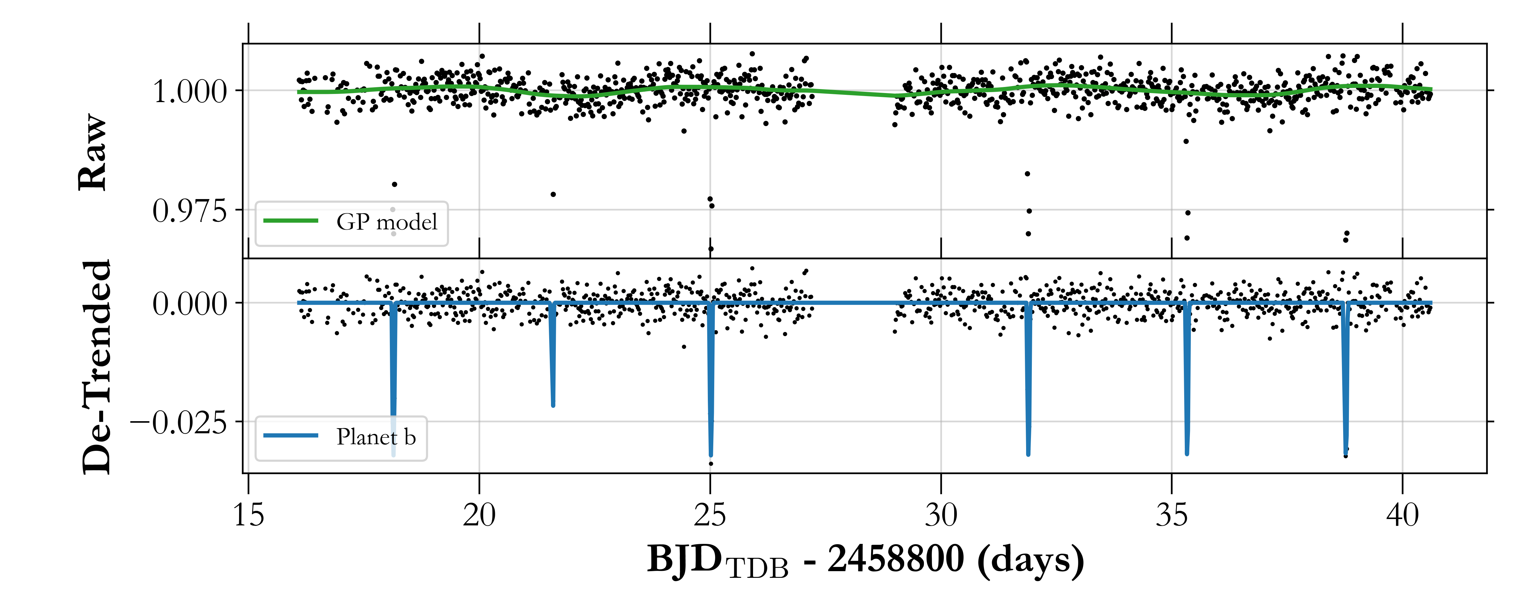
Figure 1: Long cadence (30 minute) time series TESS eleanor photometry from Sector 19, along with a stellar rotation GP kernel (RotationTerm from celerite2) in green. The detrended photometry is shown in the bottom panel, with the TOI-3757 b transits overlaid in blue.

2 Observations

2.1 TESS

TOI-3757 (TIC-445751830, 2MASS J06040089+5501126, Gaia EDR3 996878131494639488, UCAC4 726-038940) is an M0 dwarf observed by TESS in Sector 19 in Camera 2 from 2019 November 27 to 2019 December 24 at $\sim 30$ minute cadence (Figure 1). The planet candidate was identified using the Quick Look Pipeline (QLP) algorithm developed by Huang et al. (2020), under the ‘faint-star search’ (Kunimoto et al., 2021) with a period of $\sim 3.43$ d.

We extract the photometry from the TESS full-frame images using eleanor (Feinstein et al., 2019), which uses the TESScut service to obtain a cut-out of $31\times 31$ pixels from the calibrated full-frame images centered on TOI-3757. The TESS light curve is derived from the CORR_FLUX values, in which eleanor uses linear regression with pixel position, measured background, and time to remove signals correlated with these parameters. The final aperture is a $2\times 1$ rectangle centered on TOI-3757 and was selected by minimizing the combined differential photometric precision (CDPP) after the data was binned in 1 hour timescales. The CDPP is formally the RMS of the photometric noise on transit timescales, and was originally defined for Kepler (Jenkins et al., 2010). We obtain a CDPP of 2730 ppm for the TESS photometry.

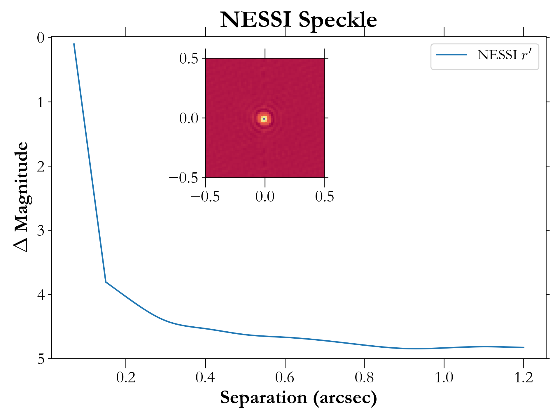
Figure 2: 5$\sigma$ contrast curve for TOI-3757 observed from NESSI in the Sloan $r^{\prime}$filter showing no bright companions within $1.2^{\prime\prime}$ from the host star. The $r^{\prime}$ image is shown as an inset 1$\arcsec$ across.

2.2 Ground based photometric follow up

2.2.1 RBO

We observed a transit of TOI-3757 b on the night of 2021 November 17 using the $0.6\,\mathrm{m}$ telescope at the Red Buttes Observatory (RBO) in Wyoming (Kasper et al., 2016). The telescope is a f/8.43 Ritchey-Chrétien Cassegrain constructed by DFM Engineering, Inc, and it is currently equipped with an Apogee Alta F16 camera.

The target rose from an airmass of 1.20 at the start of the observations to a minimum airmass of 1.02 and then set to an airmass of 1.04 at the end of the observations. We performed defocussed observations using the Bessell I filter (Bessell, 1990) exposure times of $240\,\mathrm{s}$. In the $2\times 2$ binning mode, the $0.6\,\mathrm{m}$ at RBO has a gain of $1.39\,\mathrm{e/ADU}$, a plate scale of $0.73\arcsec$, and a readout time of approximately $2.4\,\mathrm{s}$.

For the final reduction, we selected a photometric aperture of 13 pixels (9.5$\arcsec$) with a sky annulus of inner and outer radius of 23 pixels (16.8$\arcsec$) and 35 pixels (25.5$\arcsec$), respectively. We obtain an RMS precision of $\sim 1750$ ppm on the RBO photometry, after subtracting the transit model (Figure 6).

We observed TOI-3757 on the night of 21 December 2021 using the NN-Explore Exoplanet Stellar Speckle Imager (NESSI) on the WIYN 3.5m telescope at Kitt Peak National Observatory to search for faint background stars and nearby stellar companions. A 9-minute sequence of 40 ms diffraction-limited exposures was collected using the Sloan $r^{\prime}$ filter on NESSI. The speckle images were reconstructed following the procedures described in Howell et al. (2011). No stellar sources were detected down to a magnitude limit of $\Delta r^{\prime}$ = 4.0 at separations $>0.2^{\prime\prime}$, as shown in Figure 2.

2.3 Radial velocity follow-up

2.3.1 HPF

TOI-3757 was observed using HPF (Mahadevan et al., 2012, 2014) starting 2021 September 1. HPF is a near-infrared ($8080-12780$ Å), high resolution fiber-fed (Kanodia et al., 2018) precision RV spectrograph with exceptional environmental stability (Stefansson et al., 2016) located at the 10-meter Hobby-Eberly Telescope (HET) at McDonald Observatory, Texas. HET is a fixed-altitude telescope with a roving pupil design, and is fully queue-scheduled, where all the observations are executed by the HET resident astronomers (Shetrone et al., 2007). Using the algorithms described in the package HxRGproc (Ninan et al., 2018), we correct for bias, non-linearity, cosmic rays, and calculate the slope/flux and variance images from the raw HPF data. While HPF has the capability for simultaneous calibration using a NIR Laser Frequency Comb (LFC; Metcalf et al., 2019), due to the faintness of our target we chose to avoid simultaneous calibration to minimize the impact of scattered calibrator light in the science target spectra. Instead, we obtain a wavelength solution for the target exposures by interpolating the wavelength solution from other LFC exposures on the night of the observations. This helps correct for the well-calibrated instrument drift (Stefansson et al., 2020). This method has been shown to enable precise wavelength calibration and drift correction with a precision of $\sim 30$ $\textrm{cm~{}s}^{-1}$ per observation, a value much smaller than our estimated per observation RV uncertainty (instrumental + photon noise) for this object of 34 $\textrm{m~{}s}^{-1}$ (in 969 s exposures, and 23 $\textrm{m~{}s}^{-1}$ in binned 30 minute exposures).

Table 1: RVs (binned in $\sim$ 30 minute exposures) of TOI-3757. We include this table in a machine readable format along with the manuscript.

$\,\mathrm{BJD_{TDB}}$	RV	$\sigma$	Instrument
(d)	$\textrm{m~{}s}^{-1}$	$\textrm{m~{}s}^{-1}$
2459458.98300	-28.29	22.93	HPF
2459466.97200	42.47	24.02	HPF
2459472.95600	-11.67	23.40	HPF
2459489.92300	-62.93	21.99	HPF
2459503.87500	-36.31	28.99	HPF
2459506.86400	-71.04	23.27	HPF
2459507.87000	-22.90	20.91	HPF
2459509.85300	-50.03	23.73	HPF
2459512.83800	-75.03	22.47	HPF
2459513.83100	-109.27	28.70	HPF
2459516.84000	-96.78	18.73	HPF
2459517.83600	-52.47	19.65	HPF
2459532.80200	-2.53	26.69	HPF
2459533.78400	-67.68	28.71	HPF
2459551.75800	-139.99	25.00	HPF
2459571.69600	-102.35	25.02	HPF
2459505.96900	-0.50	17.21	NEID
2459523.93279	-36.64	6.78	NEID
2459528.80595	66.52	10.79	NEID
2459531.81514	27.19	11.85	NEID
2459532.81927	46.97	10.55	NEID
2459534.03339	-43.36	11.05	NEID
2459546.78516	55.86	12.63	NEID
2459554.99677	-21.28	7.57	NEID
2459582.88049	19.91	12.05	NEID
2459585.89929	-20.71	8.26	NEID
2459589.89730	-1.91	11.30	NEID

We follow the method described in Stefansson et al. (2020) to derive the RVs, by using a modified version of the SpEctrum Radial Velocity AnaLyser pipeline (SERVAL; Zechmeister et al., 2018). SERVAL uses the template-matching method (e.g., Anglada-Escudé & Butler, 2012), where it creates a master template from the target star observations, and determines the Doppler shift for each individual observation by minimizing the $\chi^{2}$ statistic. The master template is created using all of the HPF observations for TOI-3757, after masking out the telluric and sky-emission lines. The telluric regions are identified by a synthetic telluric-line mask generated from telfit (Gullikson et al., 2014), a Python wrapper to the Line-by-Line Radiative Transfer Model package (Clough et al., 2005). We use barycorrpy to perform the barycentric correction on the individual spectra, which is the Python implementation (Kanodia & Wright, 2018) of the algorithms from Wright & Eastman (2014).

We obtained a total of 25 visits on this target between 2021 September 1 and 2021 December 24, of which 9 had to be excluded from further analysis due to poor weather conditions during the observations (seeing and sky transparency). Each visit was divided into 2 exposures of 969 s each, where the median S/N of each HPF exposure was 47 per pixel at 1070 nm. The individual exposures were then binned after weighting based on SNR, with the final binned RVs being listed in Table 1.

Additionally, we observed TOI-3757 with HPF on 2021 December 12, during the transit of planet b. This observation consisted of 10x individual exposures of 649 s each, and was used to place constraints on atmospheric escape using the infrared atomic transitions of helium as a tracer (discussed further in Section 4.2). Out of an abundance of caution, we do not include this visit in our RV analysis, to avoid potential systematics from the Rossiter-McLaughlin effect (Rossiter, 1924; McLaughlin, 1924; Triaud, 2018).

2.3.2 NEID

We also observed TOI-3757 using NEID, a new ultra-precise (Halverson et al., 2016), environmentally stabilized (Robertson et al., 2019) spectrograph at the WIYN 3.5 m telescope at Kitt Peak National Observatory. NEID is a high-resolution spectrograph ($R\sim 110,000$) with an extended red wavelength coverage (380 – 930 nm; Schwab et al., 2016) ; it has a fiber-feed system similar to HPF (Kanodia et al., 2018) with three fibers — science, sky, and simultaneous calibration. For these observations we use the NEID high resolution (HR) mode with resolution $R\sim 110,000$. Between 2021 November 1 and 2022 January 10, we obtained 12 visits on TOI-3757 with NEID, of which we exclude the visit from 2021 November 2 with a S/N of 2.3 at 850 nm due to patchy clouds during the observation. Of the visits included for analysis, each consisted of an 1800 s exposure with a median S/N per 1D extracted pixel of 9.3 at 850 nm.

The NEID data was reduced using the NEID Data Reduction Pipeline (DRP), and the Level-2 1D extracted spectra were retrieved from the NEID Archive. We used a modified version of the SERVAL template-matching algorithm to obtain the NEID RVs (Stefansson et al., 2021), similar to that for HPF. The NEID RVs presented here were calculated using orders spanning 4560 – 8960 Å (order indices 40 to 104), across the central 7000 pixels which masks out the low S/N spectra outside the free spectral range. We also mask out the telluric and sky emission lines which were identified following an identical procedure to our HPF processing (Section 2.3.1), and obtain the barycentric velocities using Kanodia & Wright (2018). The final NEID RVs are listed in Table 1.

The early spectral type (M0) of TOI-3757 leads to higher RV information in the optical, than in the NIR (Bouchy et al., 2001). Coupled with negligible rotational broadening ($v$ sin $i$ $<2$ $\textrm{km~{}s}^{-1}$), this leads to NEID RVs ($R\sim 110,000$) that are much more precise than HPF ($R\sim 55,000$; Table 1, Figure 3).

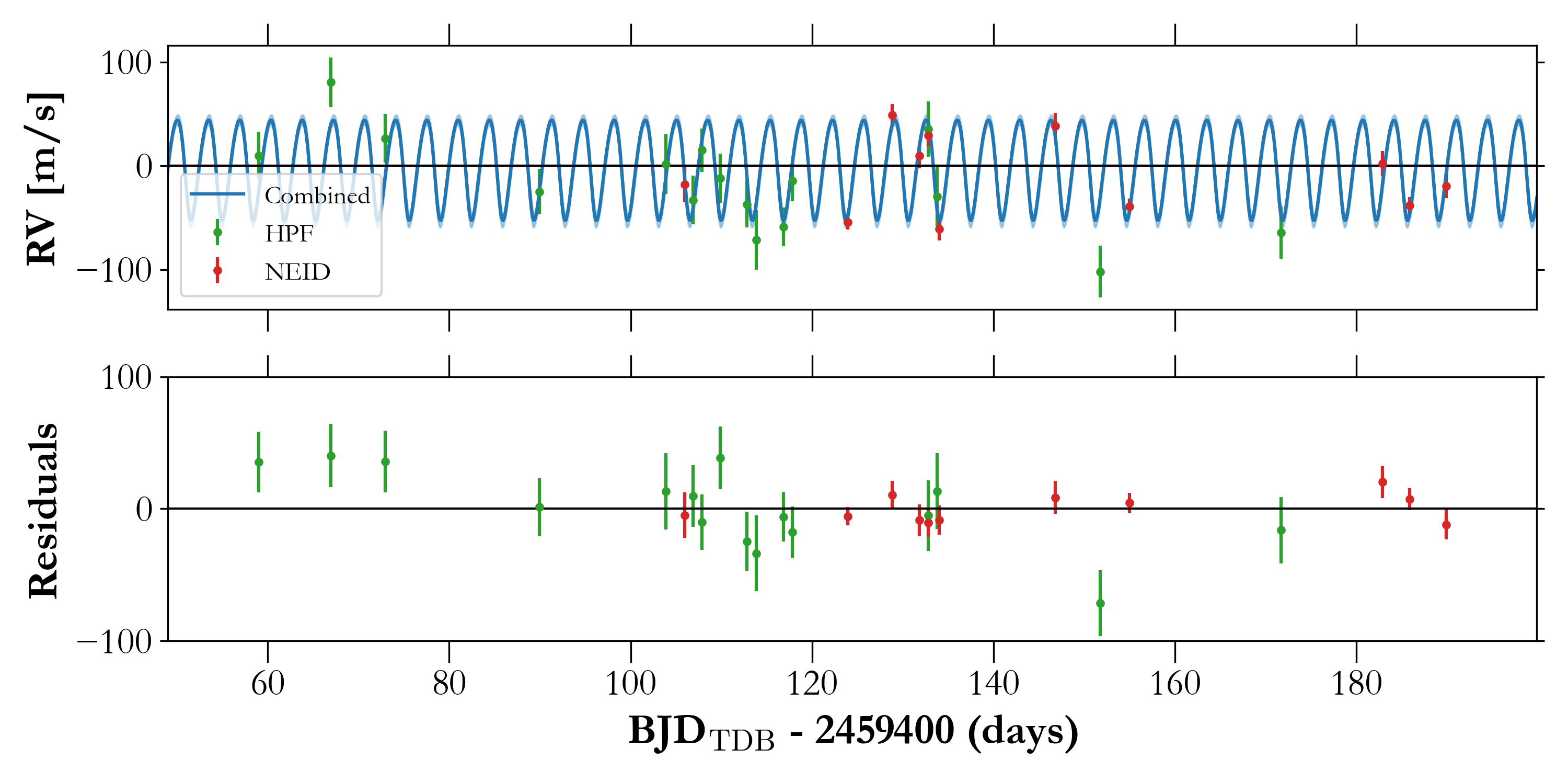
Figure 3: Time series of RV observations of TOI-3757 with HPF (green) and NEID (red). The best-fitting model derived from the joint fit to the photometry and RVs is plotted in blue, including the 16-84$\%$ confidence interval in lighter blue. The bottom panel shows the residuals after subtracting the model.

3 Stellar Parameters

3.1 Spectroscopic Parameters with HPF-SpecMatch

We use the HPF-SpecMatch package (Stefansson et al., 2020) to empirically determine stellar parameters from HPF spectra using the template matching method based on Yee et al. (2017).

The HPF-SpecMatch algorithm employs a two-step process, which uses the $\chi^{2}$ metric twice to find the library stars that best fit the target spectrum. The HPF spectral library contains 166 stars and spans the following parameter space: $2700~{}\mathrm{K}<T_{e}<6000~{}\mathrm{K}$, $4.3<\log g_{\star}<5.3$, and $-0.5<\mathrm{[Fe/H]}<0.5$.

In the first step, each stellar library spectrum is compared with the target spectrum using the $\chi^{2}$ metric and ranked from best to worst-fitting library star to the target spectrum. In the second step, only the top 5 best-fit ranked library stars are used. The $\chi^{2}$ metric is applied to assign scaling constants to each of the 5 best-fit library stars and create a composite spectrum that fits the target spectrum even more closely. These scaling constants are also used to determine a weighted average for the precise parameter estimates of effective temperature T_eff, surface gravity (log $g$), and metallicity ([Fe/H]) of the target star.

The errors we adopt for the spectroscopic parameters are determined via a leave-one-out cross-validation, broadly following the methodology in Stefansson et al. (2020). In this process, a library star of interest is removed from the rest of the stellar library pool. Then, the HPF-SpecMatch algorithm is run to estimate its stellar parameters independently of its true parameter. The difference between these calculated parameters and the true parameter values are noted. The spectral matching is performed on HPF order index 5 ($8534-8645$ Å) for TOI-3757 because this order has negligible telluric contamination. The resolution limit of HPF places a constraint of $v\sin i<2\mathrm{~{}km~{}s^{-1}}$ for TOI-3757. Table 2 presents the derived spectroscopic parameters with their uncertainties.

3.2 Model-Dependent Stellar Parameters

We derive model-dependent stellar parameters by modeling the spectral energy distribution (SED) for TOI-3757 using the EXOFASTv2 analysis package (Eastman et al., 2013). The SED fit uses the precomputed bolometric corrections in $\log g_{\star}$, T_eff, [Fe/H], and $A_{V}$ from the MIST model grids (Dotter, 2016; Choi et al., 2016).

We place Gaussian priors on the (i) broadband photometry listed in Table 2; (ii) the spectroscopic stellar parameters derived with HPF-SpecMatch, and (iii) the geometric distance calculated from Bailer-Jones et al. (2021). We set the upper limit of the visual extinction to the estimate from Green et al. (2019) calculated at the distance determined by Bailer-Jones et al. (2021). The extinction from Green et al. (2019) is converted to a visual magnitude extinction using the $R_{v}=3.1$ reddening law from Fitzpatrick (1999). Table 2 contains the stellar priors and derived stellar parameters with their uncertainties.

3.3 Galactic kinematics

We use the systemic velocity derived from HPF and proper motion from GAIA EDR3 to calculate the UVW velocities in the barycentric frame using GALPY (Bovy, 2015). We also provide the UVW velocities in the local standard of rest using the offsets from Schönrich et al. (2010). Using the BANYAN tool (Gagné et al., 2018), we classify TOI-3757 as a field star in the thin disk with very high probability ($>99\%$; Bensby et al., 2014).

3.4 Rotation Period Estimates

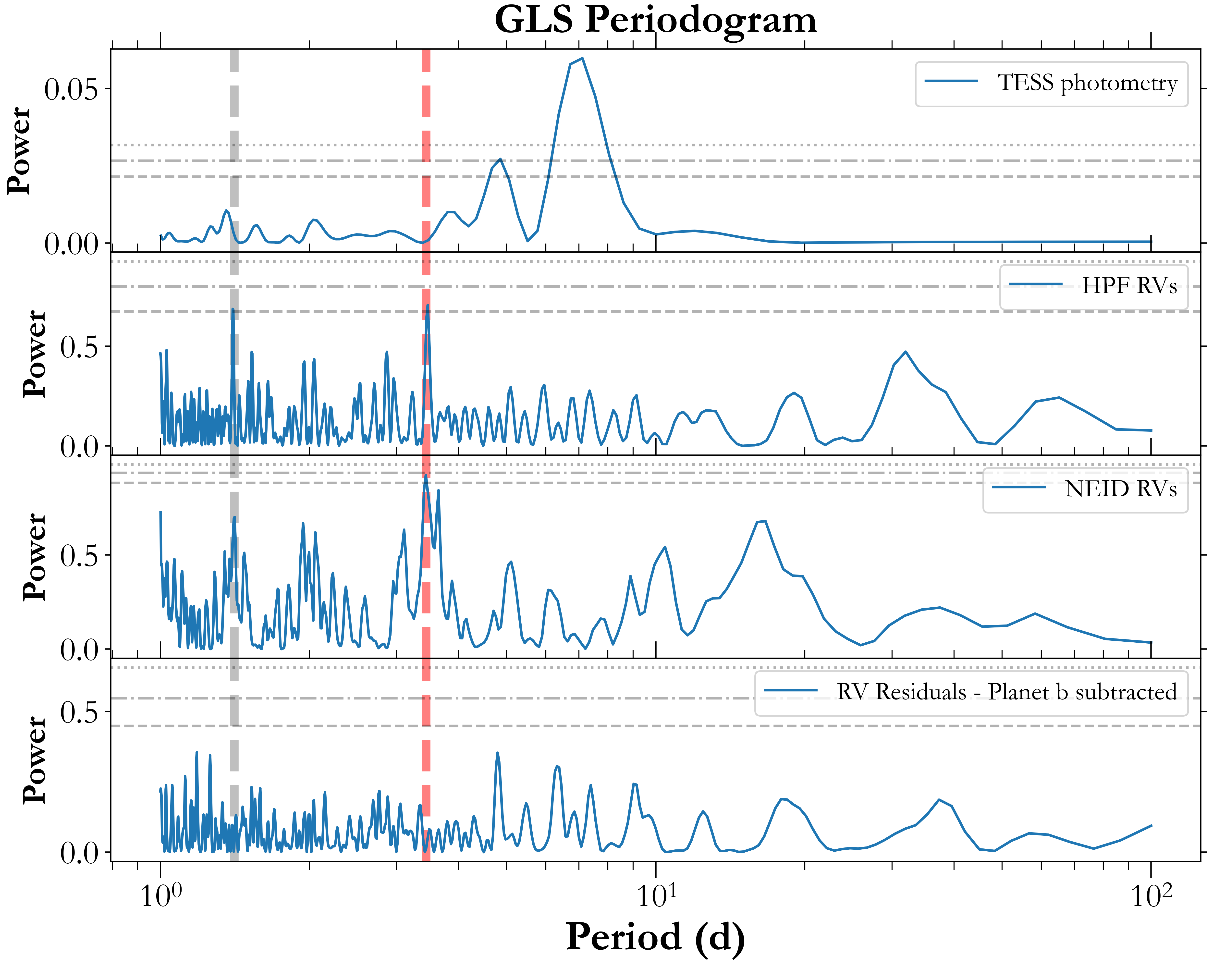
Figure 4: GLS periodogram for the different datasets. The horizontal grey lines represent the 0.1%, 1%, and 10% FAP values. The red vertical line depicts the orbital period of planet b, whereas the grey line marks its 1-day alias.

We run a generalized Lomb Scargle (GLS) periodogram (Lomb, 1976; Scargle, 1982; Zechmeister & Kürster, 2009) on the TESS photometry (after masking the transits on TOI-3757 b) using its astropy implementation, and find a significant peak ($<0.1\%$ False Alarm Probability) at $\sim 7$ days (Figure 4). This is consistent with the results from our Gaussian Process (GP) stellar rotation kernel applied to the TESS photometry, which suggest a stellar rotation period of $6.9^{+0.5}_{-0.7}$ days. This kernel consists of two simple harmonic oscillator terms – one at the rotation period, with the second one at half the period.

On further inspection using eleanor we find a similar significant peak at $\sim 7$ days for the photometry in the majority of the adjoining pixels in a 6x6 grid centered on the centroid for TOI-3757. This suggests that the periodic signal seen in the eleanor reduction of the TESS  FFI photometry is not astrophysical in origin, and TOI-3757 does not have significant rotational modulation. This is further corroborated by the lack of a detectable rotational broadening signal in the HPF spectra, using which we can place a limit of $v$ sin $i$ $<2$ $\textrm{km~{}s}^{-1}$ on the host star.

We also access publicly available data from the Zwicky Transient Facility (ZTF, Masci et al., 2019) and ASAS-SN (Kochanek et al., 2017) for this target to perform a GLS periodogram analysis, and do not detect any rotation signal present in the photometry. The photometry spans $\sim$ 800 days for ZTF and $\sim$ 1000 days for ASAS-SN. We also analyze the Ca infrared triplet from the HPF spectra, and H$\alpha$ from the NEID spectra, but do not find any periodic signals in the time series.

Table 2: Summary of stellar parameters for TOI-3757.

Parameter	Description	Value	Reference
Main identifiers:
TOI	TESS Object of Interest	3757	TESS mission
TIC	TESS Input Catalogue	445751830	Stassun
2MASS	$\cdots$	J06040089+5501126	2MASS
Gaia EDR3	$\cdots$	996878131494639488	Gaia EDR3
Equatorial Coordinates, Proper Motion and Spectral Type:
$\alpha_{\mathrm{J2016}}$	Right Ascension (RA)	06:04:00.87	Gaia EDR3
$\delta_{\mathrm{J2016}}$	Declination (Dec)	55:01:11.90	Gaia EDR3
$\mu_{\alpha}$	Proper motion (RA, $\,\mathrm{mas/yr}$)	$-9.03\pm 0.02$	Gaia EDR3
$\mu_{\delta}$	Proper motion (Dec, $\,\mathrm{mas/yr}$)	$-43.13\pm 0.02$	Gaia EDR3
$d$	Distance in pc	$177.4\pm 0.7$	Bailer-Jones
$A_{V,max}$	Maximum visual extinction	0.26	Green
Optical and near-infrared magnitudes:
$B$	Johnson B mag	$16.2\pm 0.2$	APASS
$V$	Johnson V mag	$14.8\pm 0.1$	APASS
$g^{\prime}$	Sloan $g^{\prime}$ mag	$15.5\pm 0.1$	APASS
$r^{\prime}$	Sloan $r^{\prime}$ mag	$14.2\pm 0.1$	APASS
$i^{\prime}$	Sloan $i^{\prime}$ mag	$13.5\pm 0.1$	APASS
$J$	$J$ mag	$12.00\pm 0.03$	2MASS
$H$	$H$ mag	$11.31\pm 0.03$	2MASS
$K_{s}$	$K_{s}$ mag	$11.15\pm 0.02$	2MASS
$W1$	WISE1 mag	$11.06\pm 0.02$	WISE
$W2$	WISE2 mag	$11.10\pm 0.02$	WISE
$W3$	WISE3 mag	$11.0\pm 0.1$	WISE
Spectroscopic Parametersa:
$T_{\mathrm{eff}}$	Effective temperature in $\,\mathrm{K}$	$3913\pm 56$	This work
$\mathrm{[Fe/H]}$	Metallicity in dex	$0.0\pm 0.20$	This work
$\log(g)$	Surface gravity in cgs units	$4.68\pm 0.04$	This work
Model-Dependent Stellar SED and Isochrone fit Parametersb:
$M_{*}$	Mass in $M_{\odot}$	$0.64\pm 0.02$	This work
$R_{*}$	Radius in $R_{\odot}$	$0.62\pm 0.01$	This work
$L_{*}$	Luminosity in $L_{\odot}$	$0.087\pm 0.003$	This work
$\rho_{*}$	Density in $\textrm{g~{}cm}^{-3}$	$3.7\pm 0.2$	This work
Age	Age in Gyrs	$7.1\pm 4.5$	This work
$A_{v}$	Visual extinction in mag	$0.067^{+0.078}_{-0.047}$	This work
Other Stellar Parameters:
$v\sin i_{*}$	Rotational velocity in $\textrm{km~{}s}^{-1}$	$<2$ $\textrm{km~{}s}^{-1}$	This work
$\Delta$ RV	“Absolute” radial velocity in $\textrm{km~{}s}^{-1}$	$21.86\pm 0.04$	This work
$U,V,W$	Galactic velocities in $\textrm{km~{}s}^{-1}$	$-36.12\pm 0.07,-17.81\pm 0.10,-15.82\pm 0.09$	This work
$U,V,W^{c}$	Galactic velocities (LSR) in $\textrm{km~{}s}^{-1}$	$-25.02\pm 0.85,-5.57\pm 0.69,-8.56\pm 0.61$	This work

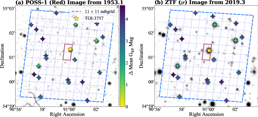
Figure 5: Panel a overlays an 11 x 11 pixel footprint from TESS Sector 19 (blue grid) on a POSS-I red image from 1953.1. TOI-3757 has a small proper motion as can be seen while comparing Panel a) and b). The TESS aperture is outlined in red and we highlight TOI-3757 with a star. No bright targets are present inside the TESS aperture with $\Delta$ G_RP $<$ 3. Panel b is similar to Panel A but with a background image from ZTF $zr$ (5600 Å– 7316 Å) from 2019 (Masci et al., 2019).

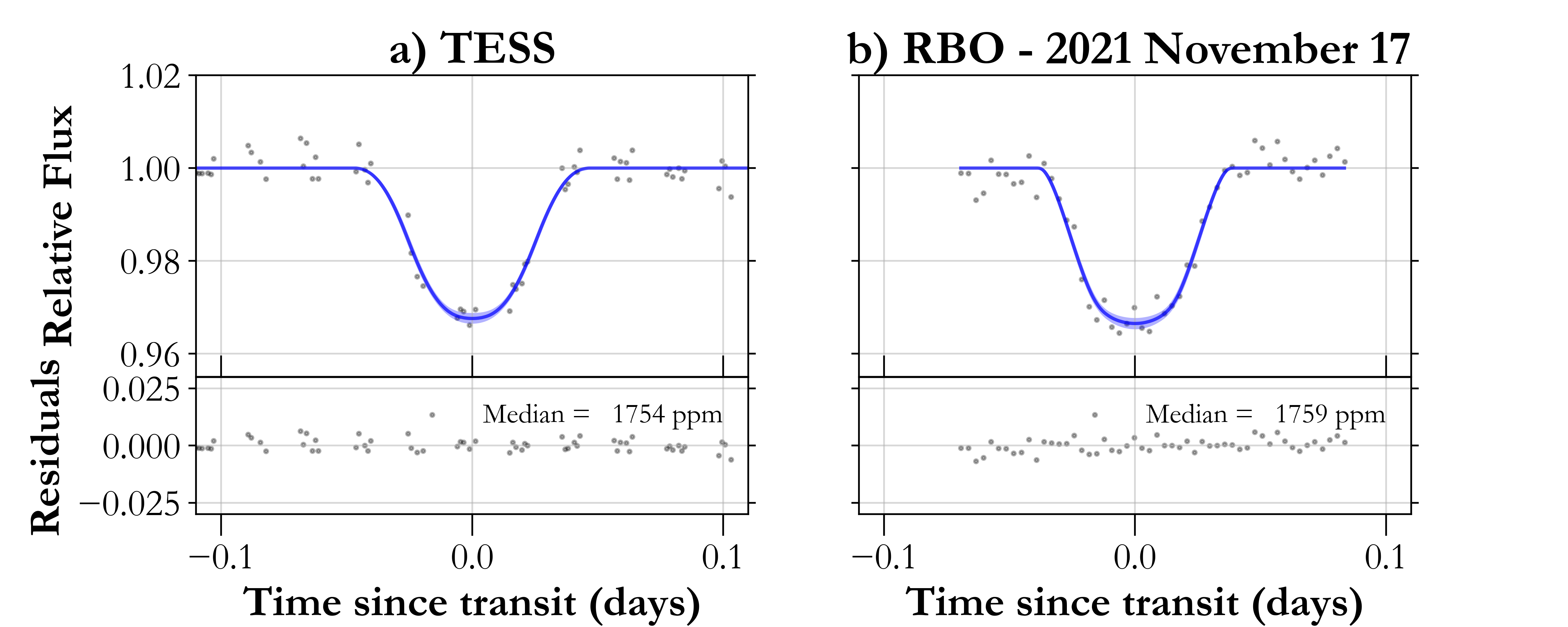
Figure 6: Photometric observations for TOI-3757 b; a) the TESS phased plot shows the detrended light curve phase-folded to the best fit orbital period, b) Ground based observations for TOI-3757 b from RBO. The raw photometery is shown in grey, with the best-fit transit solution in blue, along with the 1 $\sigma$ confidence interval shown in lighter-blue.

3.5 Ruling out Stellar Companions

3.5.1 Unresolved Stellar Companions

We try to place constraints on the presence of unresolved stellar comapnions using HPF spectra, Gaia astrometry and the RVs:

• Constraints from HPF spectra: We follow the procedure outlined in Kanodia et al. (2020), to place limits on any spatially unresolved stellar companion to TOI-3757 using the HPF spectra to quantify the lack of flux from a secondary object. We combine the spectra from a single epoch to obtain a higher S/N template for comparison, and then model the test spectra (TOI-3757) as a linear combination of a primary M dwarf (BD+29_2279) and a secondary companions (GJ 251, GJ 1156 and VB-10). The flux ratio between the secondary and primary star, $F$, is calculated as:

  $$S_{\mathrm{obs}} = A\left((1-x)S_{\mathrm{primary}}+(x)S_{\mathrm{secondary}}\right)$$ (1)

  $$F = \frac{x}{1-x}$$ (2)

  where $S_{\mathrm{obs}}$ is the observed spectrum, $S_{\mathrm{primary}}$ is the primary spectrum, $S_{\mathrm{secondary}}$ represents the secondary spectrum, and $A$ is the normalization constant. For a given primary and secondary template, we (i) perform a $\chi^{2}$ minimization to shift the secondary spectrum in velocity space, (ii) add this shifted secondary spectrum to the primary, and (iii) fit for the value of $x$ (and $A$) that best fits the observed spectrum. We perform this for a range of spectral types for the secondary from M3 to M8 spanning velocity offsets of $\pm 150$ $\textrm{km~{}s}^{-1}$. We place a conservative upper limit for a secondary companion of flux ratio $<$ 0.15 or $\Delta\rm{mag}\simeq 2.1$ for $|\Delta v|$ $>$ 5 $\textrm{km~{}s}^{-1}$, using HPF order index 17 spanning $10450-10580$ Å. The lower limit coincides with HPF’s spectral resolution ($R\sim 55,000\approx 5.5$ $\textrm{km~{}s}^{-1}$). At lower velocity offsets, the degeneracy between the primary and secondary spectra prevents any meaningful flux ratio constraints

• Constraints from Gaia astrometry: GAIA EDR3 (Lindegren et al., 2020) provides an additional astrometric constraint on the presence of unresolved bound companions using the re-normalized unit weight error (RUWE) metric. RUWE is sensitive to the change in the position of the primary target due to reflex motion caused by unresolved bound companions. For the single-star astrometric solution in use for GAIA EDR3, this astrometric motion of the primary star around the center of mass would manifest as noise (Kervella et al., 2019), especially for orbital periods much shorter than the observing baseline for GAIA EDR3 ($\sim 34$ months). The commonly accepted threshold in literature for this is RUWE $\gtrsim 1.4$, which correlates with the presence of a bound stellar companion in recent studies of stellar binaries (Penoyre et al., 2020; Belokurov et al., 2020; Gandhi et al., 2021). For TOI-3757, GAIA EDR3 reports a RUWE of $\sim 1.1$, which is in agreement with a single-star astrometric solution.

• Constraints from RVs: We use the joint fit of the photometry and radial velocity to estimate the planetary and system properties (Section 4.1). We also include a linear RV trend in the orbital solution while fitting the RVs, and note this to be consistent with 0, where the RV trend $\sim$ -0.23${}^{+4.76}_{-4.89}$ ($\textrm{m~{}s}^{-1}$ yr^-1). The residuals to this fit (Shown in Figure 3), are also analyzed with a GLS periodogram and show no significant signals (Figure 4), indicating the absence of any long-period bound companions over our observing baselines ($\sim 100$ days).

3.5.2 Resolved Stellar Companions

Figure 5 presents a comparison of the region contained in the $11\times 11$ pixel footprint from Sector 19 using a Palomar Observatory Sky Survey (POSS-1; Harrington, 1952; Minkowski & Abell, 1963) image from 1951 and a ZTF (Masci et al., 2019) image from 2019. The POSS-1 plate images were taken with Eastman 103a-E spectroscopic plates in conjunction with a No. 160 red plexiglass filter with a bandpass between 6000 – 6700 Å, and have a limiting magnitude of $R\sim 19$ (Harrington, 1952). TOI-3757 has low proper-motion, and the change in coordinates between the two epochs is negligible. There are no bright targets with $\Delta$ G_RP $<$ 3 present in the $2\times 1$ TESS aperture. There are a few targets with $\Delta$ G_RP $<$ 4, that may dilute the TESS transit. We use the ground based photometry to estimate the dilution term for the TESS photometry. Additionally, using the NESSI observations we are able to rule out stellar sources with a $\Delta r^{\prime}<4.0$ at separations $>0.2^{\prime\prime}$.

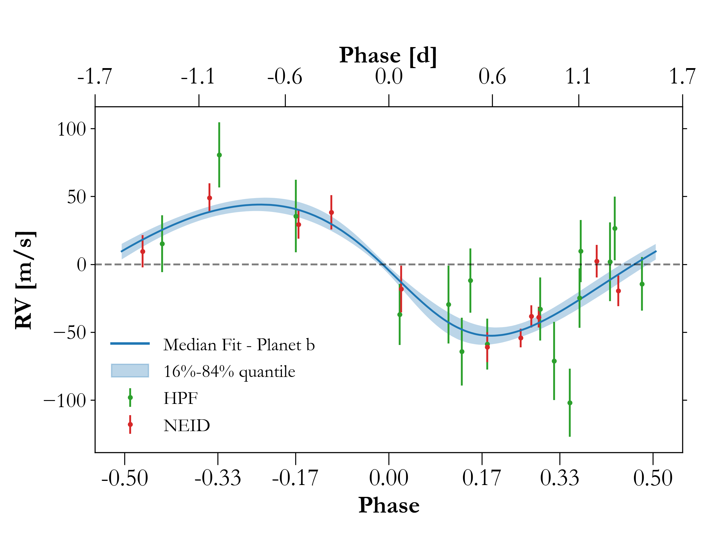
Figure 7: HPF + NEID RV observations phase folded on the best fit orbital period from the joint fit from Section 4.1. The best fit model is shown in the solid line, whereas the $1\sigma$ confidence intervals are shown in lighter blue.

4 Data Analysis

4.1 Joint Fitting of Photometry and RVs

Table 3: Derived Parameters for the TOI-3757 System.

Parameter	Units	Valuea
Orbital Parameters:
Orbital Period	$P$ (days)	3.438753$\pm$0.000004
Eccentricity	$e$	0.14$\pm 0.06$
Argument of Periastron	$\omega$ (degrees)	130$\pm 23$
Semi-amplitude Velocity	$K$ ($\textrm{m~{}s}^{-1}$)	49.24$\pm 5.07$
Systemic Velocityb	$\gamma_{\mathrm{HPF}}$ ($\textrm{m~{}s}^{-1}$)	-37.91${}^{+7.80}_{-7.85}$
	$\gamma_{\mathrm{NEID}}$ ($\textrm{m~{}s}^{-1}$)	17.58$\pm 4.15$
RV trend	$dv/dt$ ($\textrm{m~{}s}^{-1}$ yr-1)	-0.20${}^{+4.96}_{-4.94}$
RV jitter	$\sigma_{\mathrm{HPF}}$ ($\textrm{m~{}s}^{-1}$)	17.71${}^{+10.01}_{-9.49}$
	$\sigma_{\mathrm{NEID}}$ ($\textrm{m~{}s}^{-1}$)	5.82${}^{+5.66}_{-3.99}$
Transit Parameters:
Transit Midpoint	$T_{C}$ (BJDTDB)	2458838.77148${}^{+0.00062}_{-0.00061}$
Scaled Radius	$R_{p}/R_{*}$	0.1769${}^{+0.0056}_{-0.0065}$
Scaled Semi-major Axis	$a/R_{*}$	13.26${}^{+0.26}_{-0.25}$
Orbital Inclination	$i$ (degrees)	86.76${}^{+0.23}_{-0.20}$
Transit Duration	$T_{14}$ (days)	0.0800${}^{+0.0038}_{-0.0030}$
Photometric Jitterc	$\sigma_{TESS}$ (ppm)	$2569_{-59}^{+62}$
	$\sigma_{\mathrm{RBO20211117}}$ (ppm)	$2953_{-283}^{+332}$
Limb Darkeningd	$u_{1,\rm{TESS}}$, $u_{2,\rm{TESS}}$	$0.39^{+0.41}_{-0.28}$, $0.10^{+0.38}_{-0.33}$
	$u_{1,\rm{RBO20211117}}$, $u_{2,\rm{RBO20211117}}$	$0.59^{+0.43}_{-0.40}$, $0.07^{+0.43}_{-0.41}$
Dilutione	$D_{\mathrm{TESS}}$	0.994$\pm 0.053$
Planetary Parameters:
Mass	$M_{p}$ (M⊕)	85.3${}^{+8.8}_{-8.7}$
Radius	$R_{p}$ (R⊕)	12.0${}^{+0.4}_{-0.5}$
Density	$\rho_{p}$ ($\textrm{g~{}cm}^{-3}$)	0.27${}^{+0.05}_{-0.04}$
Semi-major Axis	$a$ (AU)	0.03845$\pm 0.00043$
Average Incident Fluxf	$\langle F\rangle$ ($\,\mathrm{10^{5}\ W/m^{2}}$)	0.75$\pm$0.05
Planetary Insolation	$S$ (S⊕)	55.4$\pm 3.8$
Equilibrium Temperatureg	$T_{\mathrm{eq}}$ (K)	759$\pm 13$

We perform a joint fit of the photometry (TESS + ground based sources), and the RVs (HPF + NEID) using the Python packge exoplanet, which builds upon PyMC3, the Hamiltonian Monte Carlo (HMC) package (Salvatier et al., 2016). The exoplanet package uses starry (Luger et al., 2019; Agol et al., 2020) to model the planetary transits, using the analytical transit models from Mandel & Agol (2002), and a quadratic limb-darkening law. These limb-darkening priors are implemented in exoplanet using the reparameterization from Kipping (2013) for uninformative sampling. We fit each phased transit (Figure 6) with separate limb-darkening coefficients. Our likelihood function for the TESS photometry includes the GP kernel to model the stellar rotation signal. To account for the long-cadence photometry from TESS, exoplanet (Foreman-Mackey et al., 2021a) oversamples the time series while evaluating the model.

We model the RVs using a standard Keplerian model, where we let the eccentricity float. We include a separate RV offset for each instrument (HPF and NEID), along with a common linear RV trend to account for long term drifts. For the joint modelling of the photometry + RVs, we also include a simple white-noise model in the form of a jitter term that is added in quadrature to the measurement errors from each dataset.

Using scipy.optimize, we find the initial maximum a posteriori (MAP) parameter estimates, which uses the default BFGS algorithm (Broyden–Fletcher–Goldfarb–Shanno algorithm; Broyden, 1970; Fletcher, 1970; Goldfarb, 1970; Shanno, 1970). These parameter estimates are then used as the initial conditions for parameter estimation using “No U-Turn Sampling” (NUTS, Hoffman & Gelman, 2014), implemented for the HMC sampler PyMC3, where we check for convergence using the Gelman-Rubin statistic ($\hat{\text{R}}\leq 1.1$; Ford, 2006).

The final derived planet parameters from the joint fit are included in Table 3, with the phased RVs shown in Figure 7. We obtain a $\sim 10\sigma$ mass for TOI-3757 b of 85.3${}^{+8.8}_{-8.7}$ M_⊕, and a radius of 12.0${}^{+0.4}_{-0.5}$ R_⊕.

From the joint RV + photometry fit we obtain an eccentricity of 0.14$\pm 0.06$, which is consistent with the eccentricity estimate derived from the RBO photometry using the photo-eccentric effect (Dawson & Johnson, 2012). Here, we compare the stellar density obtained from isochrones and SED fitting in Section 3, to that from the measured transit duration, which is affected by the eccentricity of this orbit. Using this comparison, we measure the eccentricity of the orbit from a joint fit of the TESS and RBO photometry to be 0.12${}^{+0.31}_{-0.09}$. This is consistent (to within 1$\sigma$) of the eccentricity derived from the joint RV + photometry fit (Table 3).

4.2 Upper limit on Helium 10830 Å absorption

The low bulk density of this planet makes it a promising candidate to detect mass-loss via atmosphere escape. We observed TOI-3757 b during its transit with HPF (described in Section 2.3.1), to constrain the absorption in the He 10830 Å  triplet due to the planetary exosphere. Not only does HET’s fixed-altitude design drastically reduce the number of transits observable with HPF, but also the stellar barycentric velocity shifts the helium triplet feature against the bright hydroxyl sky emission lines. Considering these restrictions, we observed the best available transit of TOI-3757 b with HPF in December 2021.

The individual spectra were sky subtracted using the simultaneous sky spectra obtained via an adjacent sky fiber (Kanodia et al., 2018). Conservatively, we inflate the errorbars in the pixels that are corrected for sky emission lines to avoid potential systematics. Telluric correction was not performed on this spectra, since the wavelength region of interest for He 10830 Å  detection was well outside the telluric absorption lines. We considered all spectra taken 1.9 hours (one full transit duration) away from transit midpoints in the November and December 2021 for the out-of-transit spectra. The individual out-of-transit spectra were then combined by weighted averaging to obtain a high signal-to-noise ratio template spectrum of the star. Individual in-transit spectra were then divided by this template to obtain a set of transmission (or ratio) spectra. These ratio spectra were then aligned to the planet’s rest frame (based on the orbit model) and combined by weighted average to obtain the final transmission spectrum shown in Figure 8. No statistically significant He 10830 Å  absorption signal was detected.

For calculating an upper limit, we used a Gaussian absorption line model with an FWHM width of 0.89 Å. This is the typical width of the reported helium detections in the literature across different planets . For a circular orbit, we obtain an upper limit on the maximum depth of the line as 6.9% (with 90% confidence; see Figure 8). If we consider an eccentricity of 0.14 and argument of periastron to be 130 degrees, the net radial velocity of the planet during the transit is redshifted by 11.2 km/s in comparison to the circular orbit. This places the expected planetary signal on top of a bright hyroxyl sky emission line. Therefore, an eccentric orbit ephemeris precludes us from placing any meaningful upper limit. With this caveat, while our upper limit shows the signal is weaker than some of the strongest known signal in exoplanets (Allart et al., 2019; Kirk et al., 2020), we encourage future spectroscopic and photometric observations to place tighter limits on the presence of He 10830 Å  absorption in TOI-3757.

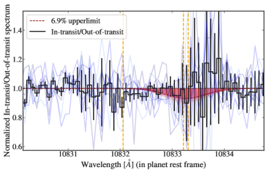
Figure 8: The ratio of the in-transit spectra and out-of-transit TOI-3757 spectra. The blue curves are the three individual ratio spectra from the transit epoch, whereas the black curve is the weighted average of the three. The x-axis shows vacuum wavelength in the planet’s rest frame at mid-transit. The rest vacuum wavelengths of the He 10830 Å, triplet lines in planet’s rest frame are marked by dashed vertical orange lines. We do not detect any significant absorption in the planetary spectra at these wavelengths. The results of our MCMC fit of the strongest doublet lines in the He 10830 Å triplet using a Gaussian model of width 0.89 Å  are shown by the red curves in the lower panel and the 6.9% upper-limit is shown by the dashed red curve overlaid on the MCMC results.

5 Discussion

5.1 TOI-3757 b: A low density gas giant

TOI-3757 b is shown in Figure 9 with respect to other M dwarf giant planets ($R_{p}>4$ $R_{\oplus}$) with mass measurements at 3$\sigma$ or higher. The data is taken from the NASA Exoplanet Archive (Akeson et al., 2013), and includes recent M dwarf transiting planets discovered by TESS. While TOI-3757 b is Jovian in size ($\sim 1.05~{}R_{J}$), its mass is about one-quarter that of Jupiter ($\sim 0.26~{}M_{J}$); due to this TOI-3757 b has the lowest density ($\rho\sim$ 0.27 $\textrm{g~{}cm}^{-3}$) hitherto of M dwarf planets with precise mass and radius measurements ($>3\sigma$).

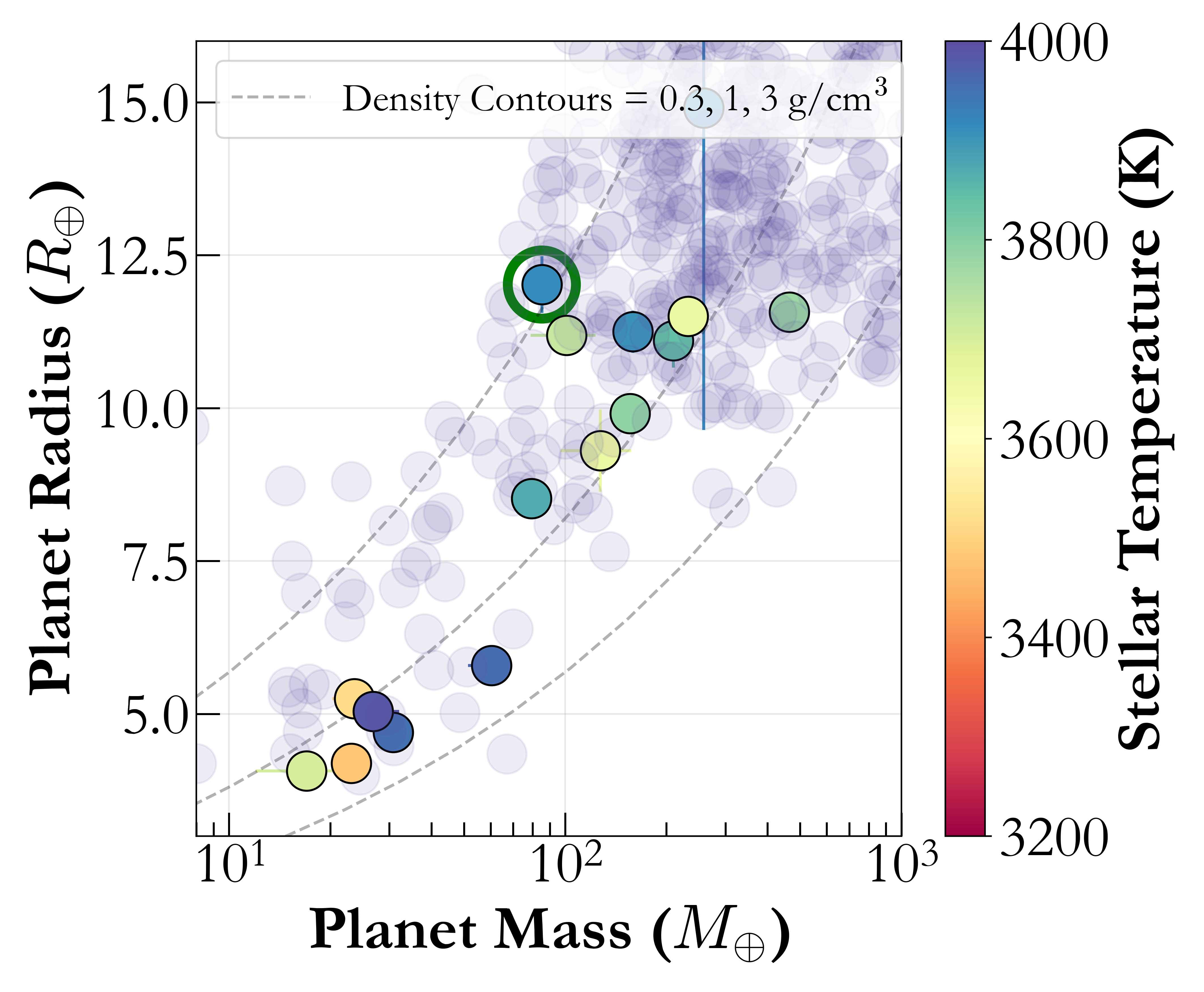
Figure 9: We show TOI-3757 b (circled in green) in a mass-radius plane alongside other M dwarf planets (coloured by the T_eff). We also include planets around FGK stars in the background, along with density contours for 0.3, 1, 3 $\textrm{g~{}cm}^{-3}$. TOI-3757 b is the lowest density planet orbiting an M dwarf with precise mass and radius measurements.

We examine different hypotheses to explain the low density (and puffy nature) of TOI-3757 b:

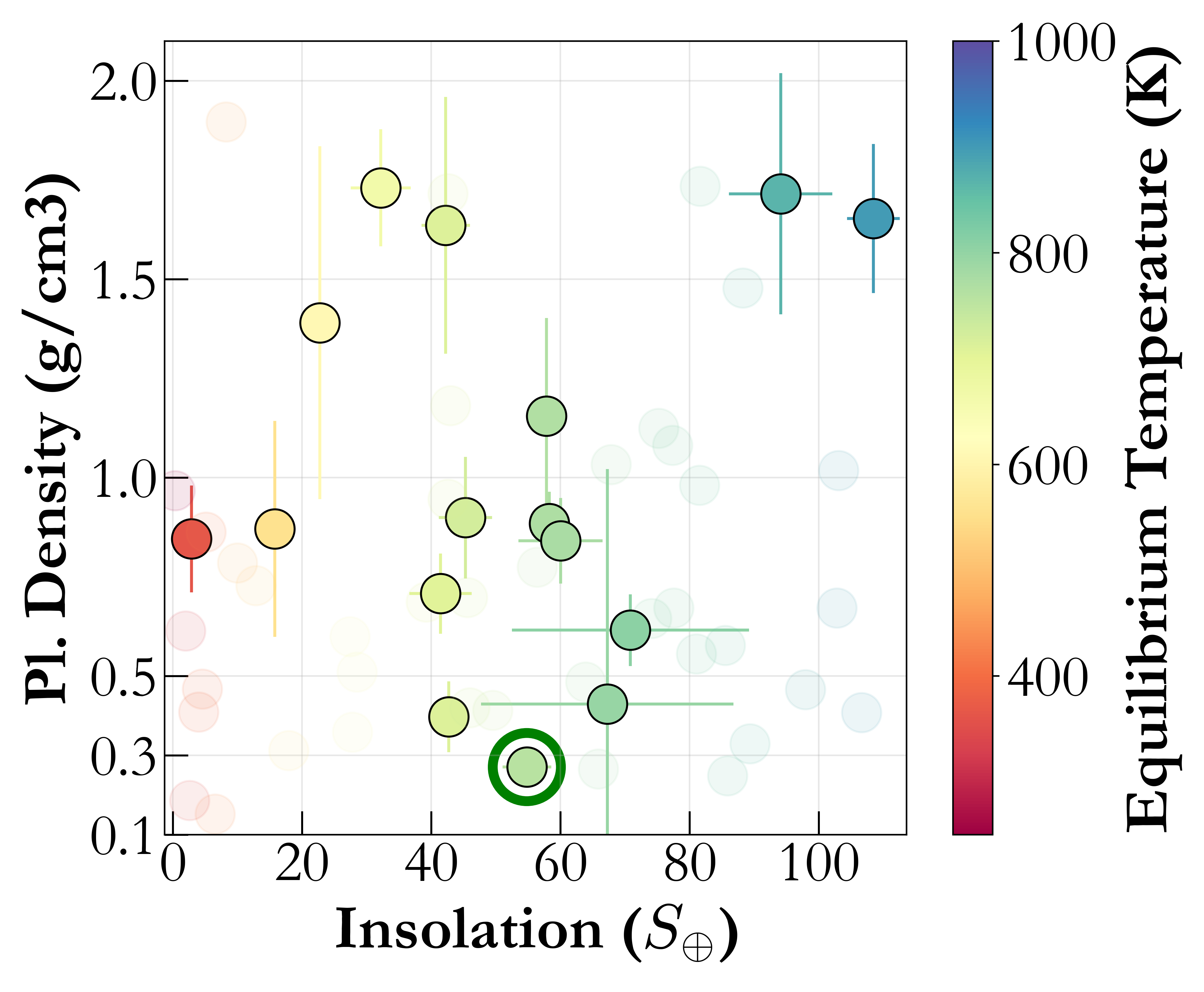
Figure 10: a) Planet density as a function of insolation flux

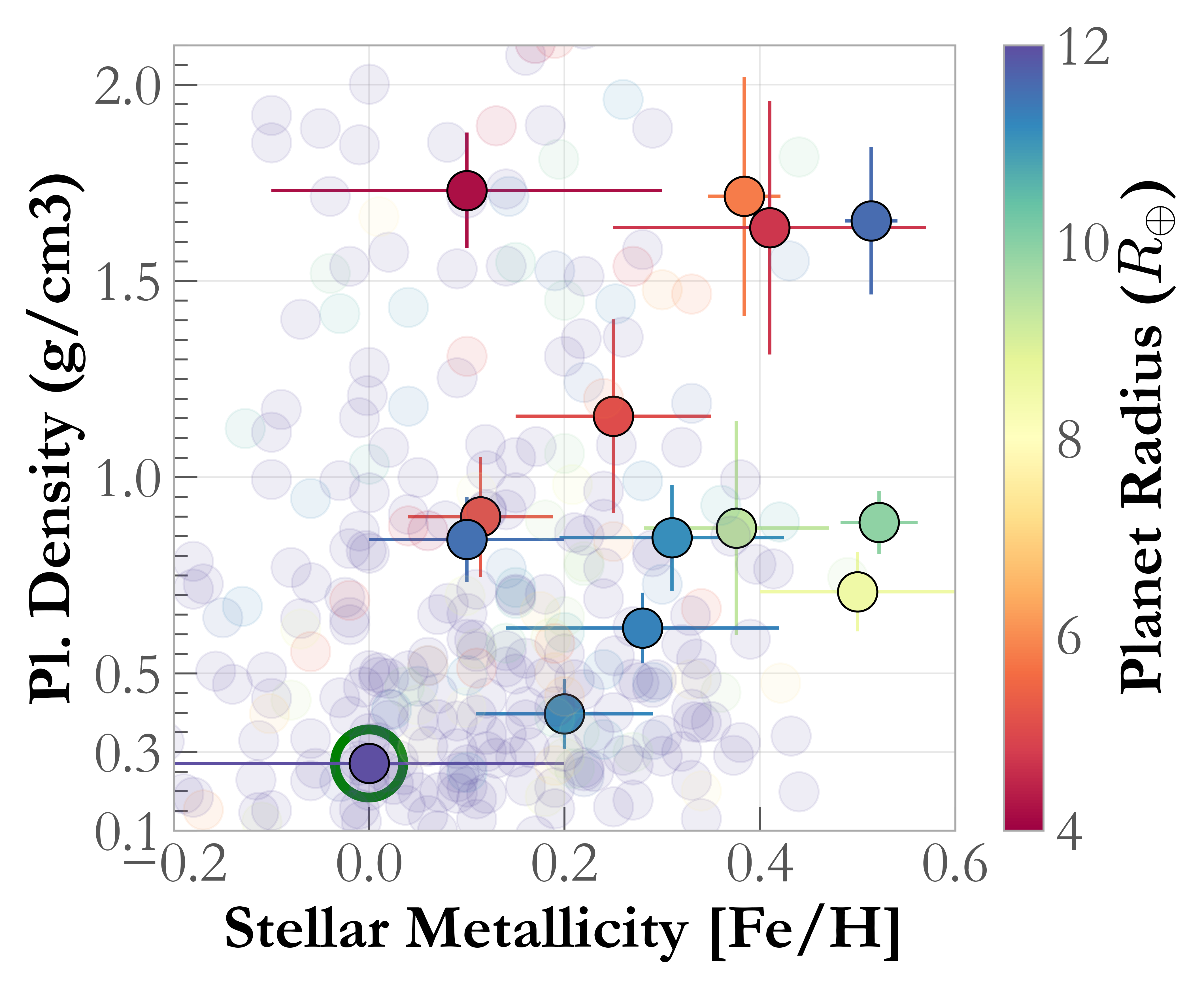
Figure 11: b) Planet density as a function of stellar metallicity

Figure 12: We show the planetary density of gas giants ($R_{p}$ $>4$$R_{\oplus}$) around M dwarfs (solid colours) as a function of stellar insolation and stellar metallicity respectively. In panel a) the markers are colour coded by the equilibrium temperature, whereas panel b) is colour coded by planetary radius. Additionally, TOI-3757 b is highlighted with a green circle. In panel a, we show that TOI-3757 b does not receive an unusually large amount of incident flux from its host star, compared to other similar gas giants. In panel b, we show that the host star has the lowest metallicity of all known gas giants around M dwarfs, which could be a potential explanation of its density.

• Stellar insolation - The inflated radii of hot-Jupiters, i.e. the so-called radius-anomaly, is primarily explained by the high stellar insolation flux incident on these planets with typical equilibrium temperatures $>1000$ K (Thorngren & Fortney, 2018). Here, a fraction of the absorbed energy from the host star is transported deep into the planetary atmosphere, which then through various mechanisms can cause its inflation. However as seen in Figure 12a, the insolation flux incident on TOI-3757 b is not anomalously higher compared to similar M dwarf gas giants. Therefore, we consider it unlikely that the inflated nature of TOI-3757 b is due to stellar insolation.

• Low metallicity - As indicated in Figure 12b, TOI-3757 b has the lowest metallicity of all known gas giants around M dwarfs. It is important to note the caveat here that the M dwarf gas giants form a heterogeneous sample relying on different techniques for metallicity determination, and hence this must be interpreted cautiously. While we pursue a detailed discussion on the role of stellar metallicity on the formation of gas giants around M dwarfs in an upcoming manuscript (Kanodia et al. in prep.), we discuss it briefly here. Assuming that the progenitor protoplanetary disk had the same metallicity as the host star, the disk for TOI-3757 is $\sim 0.3$ dex poorer in metallicity compared to the median metallicity of the other transiting gas giants around M dwarfs (Figure 12b), albeit with the caveat that our metallicity estimate for the host star TOI-3757 has a 1$\sigma$ error of 0.2 dex. Gan et al. (2021) discuss the metallicity trends seen in the transiting M dwarf Jovian sample, which have a median metallicity of $\sim 0.3$ dex, when the sample is updated to include the Jovian planets that have been confirmed since. This directly influences the formation of the planet in two ways - i) There will be $\sim$ 2x lesser material in the disk than those of comparable gas giants with higher metallicities (10${}^{+0.3}\sim 2$) ii) Yasui et al. (2009) suggest that low-metallicity protoplanetary disks have shorter lifetimes and disperse faster (than comparable high-metallicity disks). This would further exacerbate the problem of slow formation timescales for gas-giants around M dwarfs, relative to the disk lifetime (Laughlin et al., 2004).

  The initiation of runaway gas accretion under the core-accretion theory requires the formation of a rocky core of mass $\sim 10$$M_{\oplus}$ (Pollack et al., 1996) and a envelope comparable in mass ($M_{\rm{core}}\sim M_{\rm{env}}$), in a timely manner, before the disk dissipates. Under the hypothesis that the low stellar metallicity is driving the density of TOI-3757 b, due to the two reasons mentioned above, we postulate that for such planets the process of runaway gas accretion did not initiate in a timely enough manner. This would involve a core, which though massive enough for runaway accretion, did not form quickly enough to accrete substantial gas before the disk dissipated. This would explain why TOI-3757 b could not form a planet closer to Jupiter in mass, and is a failed-Jupiter.

• Excess internal heat - We explore the possibility that TOI-3757 b’s radius is inflated by internal heating (as opposed to external insolation). Multiple studies (e.g. Bodenheimer et al., 2001; Burrows et al., 2007; Lopez & Fortney, 2014; Millholland, 2019) show that a planet’s radius is influenced by its internal heat - hotter interiors lead to “puffier” radii and thus lower densities compared to cooler interior planets of the same composition. One driver of a hotter interior is simply set by a planet’s age; younger planets naturally possess hotter interiors (Marley et al., 2007). The lack of a detectable stellar rotation period and SED fit indicate that TOI-3757 is an older star, and therefore we expect its core to have naturally cooled. If TOI-3757 b’s inflated radius is due to a hotter interior, it must be heated by some other mechanism. We investigate tidal heating created by orbital eccentricity as a method for inflating the radius of TOI-3757 b. While our eccentric orbit determination for TOI-3757 b is only at the $\sim 2\sigma$ level with an eccentricity of 0.14$\pm 0.06$, we use the framework presented in Leconte et al. (2010) and calculate a tidal-to-irradiation luminosity ratio of $\sim 0.05$ (assuming an eccentricity of 0.14, zero obliquity, and a reduced tidal quality factor — Q’ — of 10⁵). Millholland et al. (2020) find that a tidal-to-irradiation luminosity ratio of $>$10^-5 is required for potential radius inflation due to eccentricity driven tides. With a tidal luminosity ratio of 5%, TOI-3757 b could be experiencing significant tidal heating from its eccentric orbit. From this power we calculate an interior temperature of 500 K for TOI-3757 b. We also determine that any eccentricity $>$0.001 would lead to some tidal heating in TOI-3757 b and provide interior temperatures $>$200 K. Therefore, it is possible that tides are responsible for at least a part of TOI-3757 b’s radius inflation. Quantifying the full impact of tidal heating on the radius inflation however requires a detailed investigation into the interior structure of TOI-3757 b, and a better estimate of eccentricity.

• Planetary rings - Recent work by Piro & Vissapragada (2020) investigate whether rings could explain the apparent inflated radii of low density super-puffs. For rings to create the appearance of inflated radii due to deeper than expected transits, the rings would need to be at an oblique angle to the planet’s orbital plane. If a planet becomes tidally locked to its star however, the ring system must remain in the orbital plane of the planet (no tilt). In this case, we would only observe the edge on portion of the ring during transit and have a negligible impact on the overall transit depth. Using Equation 11 from Piro & Vissapragada (2020), we calculate a synchronous timescale of 5.3 Myrs for TOI-3757 b. If TOI-3757 b did possess rings, they would lie in its orbital/rotation plane and not explain the planet’s inflated radii. That said, we are viewing this system from a slightly inclined angle which may tilt the rings into our vantage point. We thus further investigate whether a ring system could remain stable given TOI-3757 b’s proximity to its star. Ohta et al. (2009) note that the Poynting-Robertson drag timescale is extremely short for close-in planets. Using Equation 17 from Ohta et al. (2009), we calculate a drag timescale between 0.1 to 5 Myrs for TOI-3757 b dependent on the assumed ring particle densities and sizes. Unless TOI-3757 b also possesses some outside method for stabilizing its ring (such as shepherding moons similar to Saturn), it cannot dynamically maintain a significant ring system.

Due to the electron degeneracy pressure, Jovian sized objects can span $\sim 100$x in mass, ranging from 0.3 $M_{J}$ (Saturn mass) to $\sim$ 80 $M_{J}$ (brown dwarfs and very-low mass stars). Therefore, 2D mass-radius relationships are unable to accurately model Jovian sized gas-giants. The low density for TOI-3757 b also makes it an outlier for mass-radius relationships such as Wolfgang et al. (2016), Chen & Kipping (2017), Ning et al. (2018) and Kanodia et al. (2019). Attempts have been made to include orbital period (or insolation) as a third dimension (Ma & Ghosh, 2021) in these models to capture the radius anomaly due to host stellar insolation (Miller & Fortney, 2011; Thorngren & Fortney, 2018). However as shown above, stellar insolation is not the driving force behind the low density for TOI-3757 b, suggesting the need for higher ($>3$) dimensional analysis including stellar metallicity or eccentricity (among others). We also use the giant planet models from Fortney et al. (2007) to predict the rocky core mass for TOI-3757 b. While we do not have a precise age estimate, the models assuming a system 1 Gyr old, predict a core mass of $\sim$ 6 $M_{\oplus}$. The models for 10 Gyr (the oldest planetary population modelled by Fortney et al., 2007) do not accommodate objects as low density as TOI-3757 b, however a planet as large as TOI-3757 b would have to have a mass of $\sim 140$ $M_{\oplus}$ (which is about 1.6x the mass of TOI-3757 b) to have a core just $\sim 1$ $M_{\oplus}$ in mass. We obtain the same result with the planetary models from Baraffe et al. (2008), which are also unable to accommodate the low density of TOI-3757 b.

5.2 Atmospheric characterization

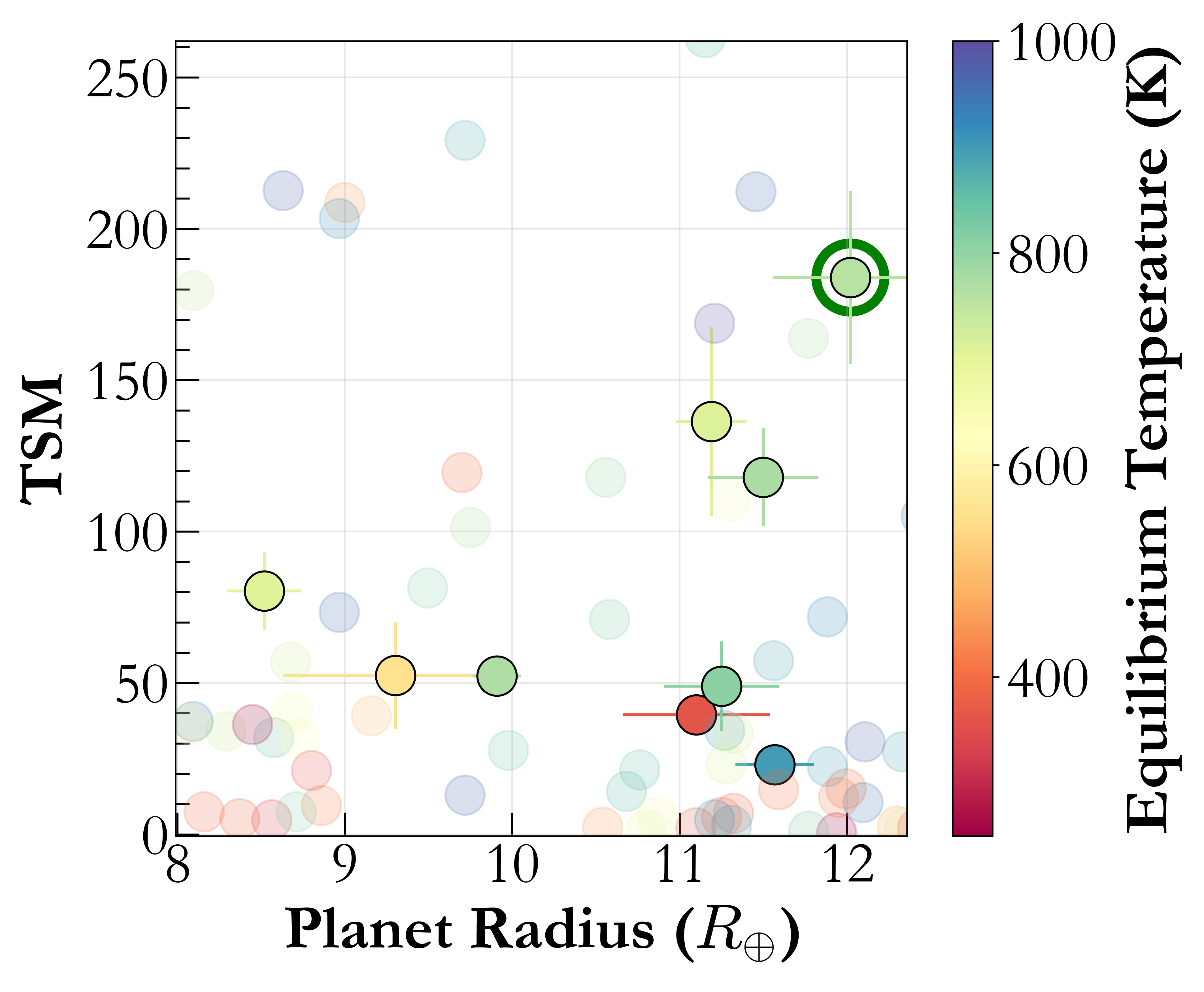
Figure 13: We show the TSM for TOI-3757 b (circled in green) as a function of planetary radius, alongside other M dwarf Saturn and Jupiter type planets ($R_{p}>6$ $R_{\oplus}$) (coloured by the equilibrium temperature). Similar planets around FGK hosts with equilibrium temperatures $<1000$ K are shown in the background. TOI-3757 b has the highest TSM among M dwarf gas giants ($R_{p}>6$ $R_{\oplus}$) with mass measurements, making it a lucrative target for atmospheric characterization, as discussed in Section 5.2.

TOI-3757 b spans multiple unique regions of parameter space, in terms of its low bulk density, and low host star metallicity (Table 4). Understanding how TOI-3757 b formed and evolved could provide the context for explaining the low density of this unusual planet. Atmospheric characterization with HST, JWST, and future instruments could provide the necessary information to test our hypotheses regarding TOI-3757 b: is its low density a result of its formational history, or is TOI-3757 b’s radius inflated from present day tidal heating?

Despite the relatively faint host star (J mag $\sim$ 12), the $\sim$ 3% transit depth and large scale height of $\sim$500 km for TOI-3757 b lend it a large TSM (transmission spectroscopy measurement; Kempton et al., 2018) of 190. As shown in Figure 13, it has one of the highest TSMs of any gas giant ($R_{p}>6$ $R_{\oplus}$) with an equilibrium temperature $<$1000 K. Beyond its detectability, TOI-3757’s mass (and scale height) is constrained to $>$9$\sigma$ precision allowing us to resolutely analyze its spectrum and removing the planet’s mass as a confounding factor during atmospheric retrievals (Batalha et al., 2019).

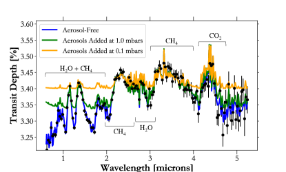
Figure 14: We create a simulated JWST/NIRSpec-Prism transmission spectrum of TOI-3757 b (assuming a single transit) using uncertainties calculated with PandExo (Batalha et al., 2017) assuming a aerosol-free 10$\times$ Solar metallicity atmosphere model (blue) generated using Exo-Transmit (Kempton et al., 2017). We also plot the same underlying composition model plus an opaque aerosol layer at 1 mbars (green) and 0.1 mbars (orange) for comparison. We assume these aerosols to be grey absorbers (i.e. no wavelength dependence absorption features). Based on PandExo simulations, we find that even with a high-altitude aerosol layer of 0.1 mbars, we should still detect water, methane, and carbon dioxide present in TOI-3757 b’s atmosphere with JWST at $\sim 9\sigma$ compared to a featureless flat spectrum.

Table 4: List of giant planets with (R${}_{p}>4$ $R_{\oplus}$) around M dwarfs, with precise masses ($>3\sigma$), and spectroscopic stellar metallicity estimates, as shown in Figure 12. Data is taken from the NASA Exoplanet Archive (Akeson et al., 2013).

Host star	Pl. Radius	Pl. Mass	Pl. Density	Orbital Period	Teff	Metallicity	Reference
	$R_{\oplus}$	$M_{\oplus}$	$\textrm{g~{}cm}^{-3}$	days	K	dex
GJ 436	4.19${}^{+0.11}_{-0.11}$	23.1${}^{+0.8}_{-0.8}$	1.73${}^{+0.148}_{-0.148}$	2.64388	3479${}^{+60}_{-60}$	0.1${}^{+0.2}_{-0.2}$	Turner et al. (2016)
LP 714-47	4.7${}^{+0.3}_{-0.3}$	30.8${}^{+1.5}_{-1.5}$	1.636${}^{+0.323}_{-0.323}$	4.05204	3950${}^{+51}_{-51}$	0.41${}^{+0.16}_{-0.16}$	Dreizler et al. (2020)
TOI-1728	5.04${}^{+0.16}_{-0.16}$	26.82${}^{+5.13}_{-5.44}$	1.155${}^{+0.247}_{-0.247}$	3.492	3985${}^{+30}_{-30}$	0.25${}^{+0.1}_{-0.1}$	Kanodia et al. (2020)
TOI-674	5.25${}^{+0.17}_{-0.17}$	23.6${}^{+3.3}_{-3.3}$	0.899${}^{+0.153}_{-0.153}$	1.97714	3514${}^{+57}_{-57}$	0.11${}^{+0.07}_{-0.07}$	Murgas et al. (2021)
TOI-532	5.79${}^{+0.18}_{-0.19}$	60.38${}^{+9.1}_{-8.77}$	1.715${}^{+0.304}_{-0.304}$	2.32665	3957${}^{+69}_{-69}$	0.38${}^{+0.04}_{-0.04}$	Kanodia et al. (2021)
TOI-3629	8.29${}^{+0.22}_{-0.22}$	82${}^{+6}_{-6}$	0.8${}^{+0.1}_{-0.1}$	3.93655	3870${}^{+90}_{-90}$	0.5${}^{+0.1}_{-0.1}$	Cañas et al. (2022b)
HATS-75	9.91${}^{+0.15}_{-0.15}$	156.05${}^{+12.4}_{-12.4}$	0.884${}^{+0.08}_{-0.08}$	2.78866	3790${}^{+5}_{-5}$	0.52${}^{+0.05}_{-0.03}$	Jordán et al. (2021)
Kepler-45	10.76${}^{+1.23}_{-1.23}$	160.49${}^{+28.6}_{-28.6}$	0.71${}^{+0.275}_{-0.275}$	2.45524	3820${}^{+90}_{-90}$	0.28${}^{+0.14}_{-0.14}$	Johnson et al. (2012)
HATS-6	11.19${}^{+0.21}_{-0.21}$	101.0${}^{+22.0}_{-22.0}$	0.397${}^{+0.089}_{-0.089}$	3.32527	3724${}^{+18}_{-18}$	0.2${}^{+0.09}_{-0.09}$	Hartman et al. (2015)
TOI-3714	11.32${}^{+0.34}_{-0.34}$	222.0${}^{+10.0}_{-10.0}$	0.85${}^{+0.08}_{-0.08}$	2.15485	3660${}^{+90}_{-90}$	0.1${}^{+0.1}_{-0.1}$	Cañas et al. (2022b)
HATS-74 A	11.57${}^{+0.24}_{-0.24}$	464.03${}^{+44.5}_{-44.5}$	1.653${}^{+0.188}_{-0.188}$	1.73186	3776${}^{+9}_{-9}$	0.51${}^{+0.03}_{-0.02}$	Jordán et al. (2021)
TOI-3757	12.02${}^{+0.44}_{-0.49}$	85.25${}^{+8.75}_{-8.67}$	0.271${}^{+0.041}_{-0.041}$	3.43875	3913${}^{+56}_{-56}$	0.0${}^{+0.2}_{-0.2}$	This work
TOI-1899	12.89${}^{+0.45}_{-0.56}$	209.77${}^{+22.25}_{-22.25}$	0.54${}^{+0.08}_{-0.08}$	29.02	3841${}^{+54}_{-45}$	0.31${}^{+0.11}_{-0.12}$	Cañas et al. (2020), Lin et al. (in prep.)

With one JWST/NIRSpec-Prism transit of TOI-3757 b, we should easily retrieve an abundance for water, methane, and carbon dioxide in its atmosphere. This combination of molecules provides a constraint on both the overall atmospheric metallicity and the C/O ratio (Moses et al., 2013; Heng, 2017); measurements that inform where in the disk this planet formed (Öberg et al., 2011) (Figure 14). We also show in Figure 14 that we should be able to observe molecular absorption features at wavelengths $>$2 microns even with an aerosol layer at 0.1 mbars. While degeneracies between aerosols and atmospheric compositions occur, we demonstrate that TOI-3757 b is a promising target for future JWST observations even if it has high-altitude aerosols present.

Aerosols (condensation clouds or photochemically created hazes) are ubiquitous across all exoplanet atmospheres; flattening or muting features in some while having little apparent effect in the atmosphere of others. By studying Titan in our own solar system, we know UV flux (even a minimal amount) drives the production of photochemical tholin hazes from the photodissociation of methane (e.g. Hörst, 2017). Even though TOI-3757 is an inactive M dwarf, it is likely still producing enough UV flux to create photochemical hazes in TOI-3757 b’s atmosphere. We would therefore hypothesize that TOI-3757 b has a hazy atmosphere. However, both Crossfield & Kreidberg (2017) and Dymont et al. (2021) found no statistically significant relationship between the UV flux of the star and the water amplitude feature observed by HST/WFC3. Alternatively, Dymont et al. (2021) do detect a tentative correlation between the planet’s density and the amplitude indicating that lower density planets may also be more hazy. This trend is greatly influenced by the four super-puff spectra, all of which appear to be featureless (Libby-Roberts et al., 2021; Chachan et al., 2020; Alam et al., 2022). TOI-3757 b’s density is similar to these super-puffs though it is $>$8$\times$ more massive.

TOI-3757 b is instead most similar to the low density sub-Saturns HAT-P-18 b and HAT-P-19 b, both of which orbit early-K dwarf stars (Hartman et al., 2011). Observed by WFC3, Tsiaras et al. (2018) retrieved a clear water abundance for HAT-P-18 b. However, when this spectrum was normalized by the scale height of the atmosphere in Dymont et al. (2021), the spectrum became near-featureless. It is therefore unclear what we can expect for TOI-3757 b in regards to aerosol formation making it an interesting target for further aerosol studies.

As discussed in Fortney et al. (2020), we may also be able to probe the interior temperature of TOI-3757 b by searching for signs of disequilibrium chemistry in the planet’s JWST spectrum. The model plotted in Figure 14 assumes chemical equilibrium; however, if TOI-3757 b possesses a hotter interior from tidal heating, methane will appear depleted compared to water which remains unaffected. Moreover, with a strong vertical diffusion coefficient (K_zz $>$10⁴) in its atmosphere, ammonia would also be present in TOI-3757 b’s JWST spectrum. If neither methane depletion or ammonia is observed, this would also place an upper limit on the interior temperature of TOI-3757, and thus a limit on the tidal heating as a source for radius inflation.

Given TOI-3757 b’s low density and extended atmosphere, the planet is potentially experiencing some atmospheric mass loss (even though TOI-3757 is fairly quiescent. Verifying this mass loss is occurring and quantifying the rate would enable us to build a picture of the planet’s atmosphere over time. The helium 10830 Å  line provides an observable mass loss tracer. As we mentioned in Section 4.2, we rule out $>$7% excess of helium absorption around the planet (assuming a circular orbit); a feature that may be due to a lack of mass loss or the lack of UV stellar flux pumping helium up to its metastable state. We note that helium was recently detected around the low density sub-Saturn HAT-P-18 b with an excess of 0.46% (Paragas et al., 2021). Considering the similarities between the two planets, it is possible that TOI-3757 b maintains an exosphere beneath the precision we achieved with a single transit on HPF. TOI-3757 b would therefore be an interesting target for future helium observations that achieve a higher precision measurement.

6 Summary

We present the discovery and confirmation of TOI-3757 b, a Jovian sized planet, characterized using a combination of space based photometry from TESS, precise RVs from HPF and NEID, ground based photometric observations from RBO, and speckle imaging from NESSI. With a planetary radius of 12.0${}^{+0.4}_{-0.5}$ $R_{\oplus}$, and mass of 85.3${}^{+8.8}_{-8.7}$ $M_{\oplus}$, TOI-3757 b has the lowest bulk density ($\rho=$ 0.27${}^{+0.05}_{-0.04}$ $\textrm{g~{}cm}^{-3}$) of all M dwarf gas giants. Additionally, its host star (TOI-3757) has the lowest stellar metallicity ($\sim$ 0.0 $\pm$ 0.20), of all M dwarfs hosting transiting gas giants. We present different hypotheses to explain the low density of the planet, with the most plausible hypotheses being a formation scenario where its low metallicity is responsible for the delayed on-set of gaseous runaway accretion before the protoplanetary disk dissipated, and an evolution mechanisms where the tidal heating causes the inflation of the planet due to its possibly slightly eccentric orbit (e $\sim$ 0.14 $\pm$ 0.06).

We observed a transit of TOI-3757 b using HPF to place upper limits on helium 10830 Å  absorption by the planetary exosphere. Finally, we discuss how the low density (and large scale height) of the planet make it an excellent target for transmission spectroscopy. With just one transit of JWST, we should be able to retrieve the abundance of water and methane in its atmosphere which would enable us to place limits on its C/O ratio. Measuring the levels of methane and ammonia would help constrain the interior temperature of TOI-3757, which can provide insight into potential tidal heating. Additionally, we discuss how TOI-3757 b can also be used to test the correlation between hazy atmospheres and planetary density.

7 Acknowledgements

We thank the anonymous referee for the valuable feedback which has improved the quality of this manuscript.

The Pennsylvania State University campuses are located on the original homelands of the Erie, Haudenosaunee (Seneca, Cayuga, Onondaga, Oneida, Mohawk, and Tuscarora), Lenape (Delaware Nation, Delaware Tribe, Stockbridge-Munsee), Shawnee (Absentee, Eastern, and Oklahoma), Susquehannock, and Wahzhazhe (Osage) Nations. As a land grant institution, we acknowledge and honor the traditional caretakers of these lands and strive to understand and model their responsible stewardship. We also acknowledge the longer history of these lands and our place in that history.

These results are based on observations obtained with the Habitable-zone Planet Finder Spectrograph on the HET. We acknowledge support from NSF grants AST-1006676, AST-1126413, AST-1310885, AST-1310875, AST-1910954, AST-1907622, AST-1909506, ATI 2009889, ATI-2009982, AST-2108512, AST-1907622, and the NASA Astrobiology Institute (NNA09DA76A) in the pursuit of precision radial velocities in the NIR. The HPF team also acknowledges support from the Heising-Simons Foundation via grant 2017-0494. The Hobby-Eberly Telescope is a joint project of the University of Texas at Austin, the Pennsylvania State University, Ludwig-Maximilians-Universität München, and Georg-August Universität Gottingen. The HET is named in honor of its principal benefactors, William P. Hobby and Robert E. Eberly. The HET collaboration acknowledges the support and resources from the Texas Advanced Computing Center. We thank the Resident astronomers and Telescope Operators at the HET for the skillful execution of our observations with HPF. We would like to acknowledge that the HET is built on Indigenous land. Moreover, we would like to acknowledge and pay our respects to the Carrizo & Comecrudo, Coahuiltecan, Caddo, Tonkawa, Comanche, Lipan Apache, Alabama-Coushatta, Kickapoo, Tigua Pueblo, and all the American Indian and Indigenous Peoples and communities who have been or have become a part of these lands and territories in Texas, here on Turtle Island.

Data presented herein were obtained at the WIYN Observatory from telescope time allocated to NN-EXPLORE through the scientific partnership of the National Aeronautics and Space Administration, the National Science Foundation, and NOIRLab. This work was supported by a NASA WIYN PI Data Award, administered by the NASA Exoplanet Science Institute. These results are based on observations obtained with NEID on the WIYN 3.5m telescope at KPNO, NSF’s NOIRLab under proposals 2021B-0035 (PI: S. Kanodia), 2021B-0435 (PI: S. Kanodia), and 2021B-2015 (PI: S. Mahadevan), managed by the Association of Universities for Research in Astronomy (AURA) under a cooperative agreement with the NSF. This work was performed for the Jet Propulsion Laboratory, California Institute of Technology, sponsored by the United States Government under the Prime Contract 80NM0018D0004 between Caltech and NASA. WIYN is a joint facility of the University of Wisconsin-Madison, Indiana University, NSF’s NOIRLab, the Pennsylvania State University, Purdue University, University of California-Irvine, and the University of Missouri. The authors are honored to be permitted to conduct astronomical research on Iolkam Du’ag (Kitt Peak), a mountain with particular significance to the Tohono O’odham. Data presented herein were obtained at the WIYN Observatory from telescope time allocated to NN-EXPLORE through the scientific partnership of NASA, the NSF, and NOIRLab.

Some of the observations in this paper made use of the NN-EXPLORE Exoplanet and Stellar Speckle Imager (NESSI). NESSI was funded by the NASA Exoplanet Exploration Program and the NASA Ames Research Center. NESSI was built at the Ames Research Center by Steve B. Howell, Nic Scott, Elliott P. Horch, and Emmett Quigley.

This work has made use of data from the European Space Agency (ESA) mission Gaia (https://www.cosmos.esa.int/gaia), processed by the Gaia Data Processing and Analysis Consortium (DPAC, https://www.cosmos.esa.int/web/gaia/dpac/consortium). Funding for the DPAC has been provided by national institutions, in particular the institutions participating in the Gaia Multilateral Agreement.

Some of the observations in this paper were obtained with the Samuel Oschin Telescope 48-inch and the 60-inch Telescope at the Palomar Observatory as part of the ZTF project. ZTF is supported by the NSF under Grant No. AST-2034437 and a collaboration including Caltech, IPAC, the Weizmann Institute for Science, the Oskar Klein Center at Stockholm University, the University of Maryland, Deutsches Elektronen-Synchrotron and Humboldt University, the TANGO Consortium of Taiwan, the University of Wisconsin at Milwaukee, Trinity College Dublin, Lawrence Livermore National Laboratories, and IN2P3, France. Operations are conducted by COO, IPAC, and UW.

Computations for this research were performed on the Pennsylvania State University’s Institute for Computational and Data Sciences Advanced CyberInfrastructure (ICDS-ACI), including the CyberLAMP cluster supported by NSF grant MRI-1626251. This content is solely the responsibility of the authors and does not necessarily represent the views of the Institute for Computational and Data Sciences.

The Center for Exoplanets and Habitable Worlds is supported by the Pennsylvania State University, the Eberly College of Science, and the Pennsylvania Space Grant Consortium.

Some of the data presented in this paper were obtained from MAST at STScI. Support for MAST for non-HST data is provided by the NASA Office of Space Science via grant NNX09AF08G and by other grants and contracts. This work includes data collected by the TESS mission, which are publicly available from MAST. Funding for the TESS mission is provided by the NASA Science Mission directorate. This research made use of the (i) NASA Exoplanet Archive, which is operated by Caltech, under contract with NASA under the Exoplanet Exploration Program, (ii) SIMBAD database, operated at CDS, Strasbourg, France, (iii) NASA’s Astrophysics Data System Bibliographic Services, and (iv) data from 2MASS, a joint project of the University of Massachusetts and IPAC at Caltech, funded by NASA and the NSF.

This research has made use of the SIMBAD database, operated at CDS, Strasbourg, France, and NASA’s Astrophysics Data System Bibliographic Services.

This research has made use of the Exoplanet Follow-up Observation Program website, which is operated by the California Institute of Technology, under contract with the National Aeronautics and Space Administration under the Exoplanet Exploration Program

CIC acknowledges support by NASA Headquarters under the NASA Earth and Space Science Fellowship Program through grant 80NSSC18K1114, the Alfred P. Sloan Foundation’s Minority Ph.D. Program through grant G-2016-20166039, and the Pennsylvania State University’s Bunton-Waller program.

SK would like to acknowledge E.H. Mason for help with this project.

This research made use of exoplanet (Foreman-Mackey et al., 2021a, b) and its dependencies (Agol et al., 2020; Foreman-Mackey et al., 2017; Foreman-Mackey, 2018; Kumar et al., 2019; Robitaille et al., 2013; Astropy Collaboration et al., 2018; Kipping, 2013; Luger et al., 2019; The Theano Development Team et al., 2016; Salvatier et al., 2016)

References

- Adams et al. (2004) Adams, F. C., Hollenbach, D., Laughlin, G., & Gorti, U. 2004, The Astrophysical Journal, 611, 360. https://ui.adsabs.harvard.edu/abs/2004ApJ...611..360A
- Agol et al. (2020) Agol, E., Luger, R., & Foreman-Mackey, D. 2020, The Astronomical Journal, 159, 123. https://ui.adsabs.harvard.edu/abs/2020AJ....159..123A
- Akeson et al. (2013) Akeson, R. L., Chen, X., Ciardi, D., et al. 2013, Publications of the Astronomical Society of the Pacific, 125, 989. http://adsabs.harvard.edu/abs/2013PASP..125..989A
- Alam et al. (2022) Alam, M. K., Kirk, J., Dressing, C. D., et al. 2022, arXiv e-prints, arXiv:2201.02686
- Allart et al. (2018) Allart, R., Bourrier, V., Lovis, C., et al. 2018, Science, 362, 1384, aDS Bibcode: 2018Sci…362.1384A. https://ui.adsabs.harvard.edu/abs/2018Sci...362.1384A
- Allart et al. (2019) —. 2019, Astronomy & Astrophysics, Volume 623, id.A58, <NUMPAGES>6</NUMPAGES> pp., 623, A58. https://ui.adsabs.harvard.edu/abs/2019A%26A...623A..58A/abstract
- Alonso-Floriano et al. (2019) Alonso-Floriano, F. J., Snellen, I. a. G., Czesla, S., et al. 2019, Astronomy & Astrophysics, Volume 629, id.A110, <NUMPAGES>7</NUMPAGES> pp., 629, A110. https://ui.adsabs.harvard.edu/abs/2019A%26A...629A.110A/abstract
- Andrews et al. (2013) Andrews, S. M., Rosenfeld, K. A., Kraus, A. L., & Wilner, D. J. 2013, The Astrophysical Journal, 771, 129, aDS Bibcode: 2013ApJ…771..129A. https://ui.adsabs.harvard.edu/abs/2013ApJ...771..129A
- Anglada-Escudé & Butler (2012) Anglada-Escudé, G., & Butler, R. P. 2012, The Astrophysical Journal Supplement Series, 200, 15. https://doi.org/10.1088%2F0067-0049%2F200%2F2%2F15
- Astropy Collaboration et al. (2018) Astropy Collaboration, Price-Whelan, A. M., Sipőcz, B. M., et al. 2018, The Astronomical Journal, 156, 123. https://ui.adsabs.harvard.edu/abs/2018AJ....156..123A
- Bailer-Jones et al. (2021) Bailer-Jones, C. A. L., Rybizki, J., Fouesneau, M., Demleitner, M., & Andrae, R. 2021, The Astronomical Journal, 161, 147. http://adsabs.harvard.edu/abs/2021AJ....161..147B
- Bailer-Jones et al. (2018) Bailer-Jones, C. A. L., Rybizki, J., Fouesneau, M., Mantelet, G., & Andrae, R. 2018, The Astronomical Journal, 156, 58. http://adsabs.harvard.edu/abs/2018AJ....156...58B
- Baraffe et al. (2008) Baraffe, I., Chabrier, G., & Barman, T. 2008, Astronomy and Astrophysics, 482, 315. http://adsabs.harvard.edu/abs/2008A%26A...482..315B
- Batalha et al. (2019) Batalha, N. E., Lewis, T., Fortney, J. J., et al. 2019, The Astrophysical Journal Letters, 885, L25. http://adsabs.harvard.edu/abs/2019ApJ...885L..25B
- Batalha et al. (2017) Batalha, N. E., Mandell, A., Pontoppidan, K., et al. 2017, Publications of the Astronomical Society of the Pacific, 129, 064501, aDS Bibcode: 2017PASP..129f4501B. https://ui.adsabs.harvard.edu/abs/2017PASP..129f4501B
- Batygin et al. (2011) Batygin, K., Stevenson, D. J., & Bodenheimer, P. H. 2011, ApJ, 738, 1
- Belokurov et al. (2020) Belokurov, V., Penoyre, Z., Oh, S., et al. 2020, Monthly Notices of the Royal Astronomical Society, 496, 1922, aDS Bibcode: 2020MNRAS.496.1922B. https://ui.adsabs.harvard.edu/abs/2020MNRAS.496.1922B
- Bensby et al. (2014) Bensby, T., Feltzing, S., & Oey, M. S. 2014, Astronomy and Astrophysics, 562, A71. http://adsabs.harvard.edu/abs/2014A%26A...562A..71B
- Bessell (1990) Bessell, M. S. 1990, Publications of the Astronomical Society of the Pacific, 102, 1181. https://ui.adsabs.harvard.edu/abs/1990PASP..102.1181B/abstract
- Bodenheimer et al. (2001) Bodenheimer, P., Lin, D. N. C., & Mardling, R. A. 2001, The Astrophysical Journal, 548, 466, aDS Bibcode: 2001ApJ…548..466B. https://ui.adsabs.harvard.edu/abs/2001ApJ...548..466B
- Bouchy et al. (2001) Bouchy, F., Pepe, F., & Queloz, D. 2001, Astronomy and Astrophysics, v.374, p.733-739 (2001), 374, 733. https://ui.adsabs.harvard.edu/abs/2001A%26A...374..733B/abstract
- Bovy (2015) Bovy, J. 2015, The Astrophysical Journal Supplement Series, 216, 29. http://adsabs.harvard.edu/abs/2015ApJS..216...29B
- Broyden (1970) Broyden, C. G. 1970, IMA Journal of Applied Mathematics, 6, 76. https://doi.org/10.1093/imamat/6.1.76
- Burn et al. (2021) Burn, R., Schlecker, M., Mordasini, C., et al. 2021, arXiv e-prints, arXiv:2105.04596. https://ui.adsabs.harvard.edu/abs/2021arXiv210504596B
- Burrows et al. (2007) Burrows, A., Hubeny, I., Budaj, J., & Hubbard, W. B. 2007, ApJ, 661, 502
- Cañas et al. (2020) Cañas, C. I., Stefansson, G., Kanodia, S., et al. 2020, The Astronomical Journal, 160, 147. http://adsabs.harvard.edu/abs/2020AJ....160..147C
- Cañas et al. (2022a) Cañas, C. I., Mahadevan, S., Cochran, W. D., et al. 2022a, The Astronomical Journal, 163, 3, aDS Bibcode: 2022AJ….163….3C. https://ui.adsabs.harvard.edu/abs/2022AJ....163....3C
- Cañas et al. (2022b) Cañas, C. I., Kanodia, S., Bender, C. F., et al. 2022b, Two gas giants transiting M dwarfs confirmed with HPF and NEID, Tech. rep., publication Title: arXiv e-prints ADS Bibcode: 2022arXiv220109963C Type: article. https://ui.adsabs.harvard.edu/abs/2022arXiv220109963C
- Chachan et al. (2020) Chachan, Y., Jontof-Hutter, D., Knutson, H. A., et al. 2020, AJ, 160, 201
- Chen & Kipping (2017) Chen, J., & Kipping, D. 2017, The Astrophysical Journal, 834, 17, aDS Bibcode: 2017ApJ…834…17C. https://ui.adsabs.harvard.edu/abs/2017ApJ...834...17C
- Choi et al. (2016) Choi, J., Dotter, A., Conroy, C., et al. 2016, The Astrophysical Journal, 823, 102, aDS Bibcode: 2016ApJ…823..102C. https://ui.adsabs.harvard.edu/abs/2016ApJ...823..102C
- Clough et al. (2005) Clough, S. A., Shephard, M. W., Mlawer, E. J., et al. 2005, Journal of Quantitative Spectroscopy and Radiative Transfer, 91, 233. http://adsabs.harvard.edu/abs/2005JQSRT..91..233C
- Collaboration et al. (2021) Collaboration, G., Brown, A. G. A., Vallenari, A., et al. 2021, Astronomy and Astrophysics, 649, A1. https://ui.adsabs.harvard.edu/abs/2021A&A...649A...1G/abstract
- Collins et al. (2017) Collins, K. A., Kielkopf, J. F., Stassun, K. G., & Hessman, F. V. 2017, The Astronomical Journal, 153, 77. http://adsabs.harvard.edu/abs/2017AJ....153...77C
- Crossfield & Kreidberg (2017) Crossfield, I. J. M., & Kreidberg, L. 2017, The Astronomical Journal, 154, 261. http://adsabs.harvard.edu/abs/2017AJ....154..261C
- Cutri et al. (2003) Cutri, R. M., Skrutskie, M. F., van Dyk, S., et al. 2003, ”The IRSA 2MASS All-Sky Point Source Catalog, NASA/IPAC Infrared Science Archive. http://irsa.ipac.caltech.edu/applications/Gator/”. http://adsabs.harvard.edu/abs/2003tmc..book.....C
- Dawson & Johnson (2012) Dawson, R. I., & Johnson, J. A. 2012, The Astrophysical Journal, 756, 122, aDS Bibcode: 2012ApJ…756..122D. https://ui.adsabs.harvard.edu/abs/2012ApJ...756..122D
- Dotter (2016) Dotter, A. 2016, The Astrophysical Journal Supplement Series, 222, 8, aDS Bibcode: 2016ApJS..222….8D. https://ui.adsabs.harvard.edu/abs/2016ApJS..222....8D
- Dreizler et al. (2020) Dreizler, S., Crossfield, I. J. M., Kossakowski, D., et al. 2020, Astronomy and Astrophysics, 644, A127. https://ui.adsabs.harvard.edu/abs/2020A&A...644A.127D/abstract
- Dymont et al. (2021) Dymont, A. H., Yu, X., Ohno, K., Zhang, X., & Fortney, J. J. 2021, arXiv e-prints, arXiv:2112.06173
- Eastman et al. (2013) Eastman, J., Gaudi, B. S., & Agol, E. 2013, Publications of the Astronomical Society of the Pacific, 125, 83. https://iopscience.iop.org/article/10.1086/669497/meta
- Endl et al. (2006) Endl, M., Cochran, W. D., Kürster, M., et al. 2006, The Astrophysical Journal, 649, 436. http://adsabs.harvard.edu/abs/2006ApJ...649..436E
- Feinstein et al. (2019) Feinstein, A. D., Montet, B. T., Foreman-Mackey, D., et al. 2019, Publications of the Astronomical Society of the Pacific, 131, 094502. https://ui.adsabs.harvard.edu/abs/2019PASP..131i4502F
- Fischer & Valenti (2005) Fischer, D. A., & Valenti, J. 2005, The Astrophysical Journal, 622, 1102, aDS Bibcode: 2005ApJ…622.1102F. https://ui.adsabs.harvard.edu/abs/2005ApJ...622.1102F
- Fitzpatrick (1999) Fitzpatrick, E. L. 1999, Publications of the Astronomical Society of the Pacific, 111, 63. http://adsabs.harvard.edu/abs/1999PASP..111...63F
- Fletcher (1970) Fletcher, R. 1970, The Computer Journal, 13, 317. https://doi.org/10.1093/comjnl/13.3.317
- Ford (2006) Ford, E. B. 2006, The Astrophysical Journal, 642, 505. http://adsabs.harvard.edu/abs/2006ApJ...642..505F
- Foreman-Mackey (2018) Foreman-Mackey, D. 2018, Research Notes of the American Astronomical Society, 2, 31, tex.adsnote: Provided by the SAO/NASA Astrophysics Data System tex.adsurl: http://adsabs.harvard.edu/abs/2018RNAAS…2a..31F
- Foreman-Mackey et al. (2017) Foreman-Mackey, D., Agol, E., Ambikasaran, S., & Angus, R. 2017, The Astronomical Journal, 154, 220, arXiv: 1703.09710. http://arxiv.org/abs/1703.09710
- Foreman-Mackey et al. (2021a) Foreman-Mackey, D., Savel, A., Luger, R., et al. 2021a, exoplanet-dev/exoplanet v0.4.4, , , doi:10.5281/zenodo.1998447. https://doi.org/10.5281/zenodo.1998447
- Foreman-Mackey et al. (2021b) Foreman-Mackey, D., Luger, R., Agol, E., et al. 2021b, The Journal of Open Source Software, 6, 3285. https://ui.adsabs.harvard.edu/abs/2021JOSS....6.3285F
- Fortney et al. (2021) Fortney, J. J., Dawson, R. I., & Komacek, T. D. 2021, Journal of Geophysical Research (Planets), 126, e06629. https://ui.adsabs.harvard.edu/abs/2021JGRE..12606629F
- Fortney et al. (2007) Fortney, J. J., Marley, M. S., & Barnes, J. W. 2007, ApJ, 659, 1661. https://ui.adsabs.harvard.edu/abs/2007ApJ...659.1661F/abstract
- Fortney et al. (2020) Fortney, J. J., Visscher, C., Marley, M. S., et al. 2020, The Astronomical Journal, 160, 288, aDS Bibcode: 2020AJ….160..288F. https://ui.adsabs.harvard.edu/abs/2020AJ....160..288F
- Gagné et al. (2018) Gagné, J., Mamajek, E. E., Malo, L., et al. 2018, The Astrophysical Journal, 856, 23. http://adsabs.harvard.edu/abs/2018ApJ...856...23G
- Gan et al. (2021) Gan, T., Lin, Z., Wang, S. X., et al. 2021, arXiv:2110.04220 [astro-ph], arXiv: 2110.04220. http://arxiv.org/abs/2110.04220
- Gandhi et al. (2021) Gandhi, P., Buckley, D. A. H., Charles, P. A., et al. 2021, Monthly Notices of the Royal Astronomical Society, doi:10.1093/mnras/stab3771, aDS Bibcode: 2021MNRAS.tmp.3450G. https://ui.adsabs.harvard.edu/abs/2021MNRAS.tmp.3450G
- Ghezzi et al. (2010) Ghezzi, L., Cunha, K., Smith, V. V., et al. 2010, The Astrophysical Journal, 720, 1290. http://adsabs.harvard.edu/abs/2010ApJ...720.1290G
- Ginsburg et al. (2019) Ginsburg, A., Sipőcz, B. M., Brasseur, C. E., et al. 2019, The Astronomical Journal, 157, 98. http://adsabs.harvard.edu/abs/2019AJ....157...98G
- Goldfarb (1970) Goldfarb, D. 1970, Mathematics of Computation, 24, 23. https://www.ams.org/mcom/1970-24-109/S0025-5718-1970-0258249-6/
- Gonzalez (1997) Gonzalez, G. 1997, Monthly Notices of the Royal Astronomical Society, 285, 403. http://adsabs.harvard.edu/abs/1997MNRAS.285..403G
- Gould et al. (2006) Gould, A., Dorsher, S., Gaudi, B. S., & Udalski, A. 2006, Acta Astronomica, 56, 1. http://adsabs.harvard.edu/abs/2006AcA....56....1G
- Green et al. (2019) Green, G. M., Schlafly, E., Zucker, C., Speagle, J. S., & Finkbeiner, D. 2019, The Astrophysical Journal, 887, 93. http://adsabs.harvard.edu/abs/2019ApJ...887...93G
- Gullikson et al. (2014) Gullikson, K., Dodson-Robinson, S., & Kraus, A. 2014, The Astronomical Journal, 148, 53. http://adsabs.harvard.edu/abs/2014AJ....148...53G
- Halverson et al. (2016) Halverson, S., Terrien, R., Mahadevan, S., et al. 2016, SPIE Proceedings Vol. 9908, 9908, 99086P. http://adsabs.harvard.edu/abs/2016SPIE.9908E..6PH
- Harrington (1952) Harrington, R. G. 1952, Publications of the Astronomical Society of the Pacific, 64, 275. http://adsabs.harvard.edu/abs/1952PASP...64..275H
- Hartman et al. (2011) Hartman, J. D., Bakos, G. Á., Sato, B., et al. 2011, ApJ, 726, 52
- Hartman et al. (2015) Hartman, J. D., Bayliss, D., Brahm, R., et al. 2015, The Astronomical Journal, 149, 166, aDS Bibcode: 2015AJ….149..166H. https://ui.adsabs.harvard.edu/abs/2015AJ....149..166H
- Henden et al. (2018) Henden, A. A., Levine, S., Terrell, D., et al. 2018, 232, 223.06, conference Name: American Astronomical Society Meeting Abstracts #232. http://adsabs.harvard.edu/abs/2018AAS...23222306H
- Heng (2017) Heng, K. 2017, Exoplanetary Atmospheres: Theoretical Concepts and Foundations
- Hoffman & Gelman (2014) Hoffman, M. D., & Gelman, A. 2014, Journal of Machine Learning Research, 15, 1593. http://jmlr.org/papers/v15/hoffman14a.html
- Hörst (2017) Hörst, S. M. 2017, Journal of Geophysical Research (Planets), 122, 432
- Howell et al. (2011) Howell, S. B., Everett, M. E., Sherry, W., Horch, E., & Ciardi, D. R. 2011, The Astronomical Journal, 142, 19, aDS Bibcode: 2011AJ….142…19H. https://ui.adsabs.harvard.edu/abs/2011AJ....142...19H
- Huang et al. (2020) Huang, C. X., Vanderburg, A., Pál, A., et al. 2020, Research Notes of the AAS, 4, 204, publisher: American Astronomical Society. https://doi.org/10.3847/2515-5172/abca2e
- Hunter (2007) Hunter, J. D. 2007, Computing in Science Engineering, 9, 90
- Ida & Lin (2004) Ida, S., & Lin, D. N. C. 2004, The Astrophysical Journal, 616, 567. http://adsabs.harvard.edu/abs/2004ApJ...616..567I
- Ida & Lin (2005) —. 2005, The Astrophysical Journal, 626, 1045. http://adsabs.harvard.edu/abs/2005ApJ...626.1045I
- Jenkins et al. (2010) Jenkins, J. M., Caldwell, D. A., Chandrasekaran, H., et al. 2010, The Astrophysical Journal, 713, L87, aDS Bibcode: 2010ApJ…713L..87J. https://ui.adsabs.harvard.edu/abs/2010ApJ...713L..87J
- Johnson & Soderblom (1987) Johnson, D. R. H., & Soderblom, D. R. 1987, The Astronomical Journal, 93, 864. https://ui.adsabs.harvard.edu/abs/1987AJ.....93..864J/abstract
- Johnson & Apps (2009) Johnson, J. A., & Apps, K. 2009, The Astrophysical Journal, 699, 933. http://adsabs.harvard.edu/abs/2009ApJ...699..933J
- Johnson et al. (2007) Johnson, J. A., Butler, R. P., Marcy, G. W., et al. 2007, The Astrophysical Journal, 670, 833. http://adsabs.harvard.edu/abs/2007ApJ...670..833J
- Johnson et al. (2012) Johnson, J. A., Gazak, J. Z., Apps, K., et al. 2012, The Astronomical Journal, 143, 111, aDS Bibcode: 2012AJ….143..111J. https://ui.adsabs.harvard.edu/abs/2012AJ....143..111J
- Jordán et al. (2021) Jordán, A., Hartman, J. D., Bayliss, D., et al. 2021, HATS-74Ab, HATS-75b, HATS-76b and HATS-77b: Four Transiting Giant Planets around K and M Dwarfs, Tech. rep., publication Title: arXiv e-prints ADS Bibcode: 2021arXiv211201928J Type: article. https://ui.adsabs.harvard.edu/abs/2021arXiv211201928J
- Kanodia et al. (2019) Kanodia, S., Wolfgang, A., Stefansson, G. K., Ning, B., & Mahadevan, S. 2019, The Astrophysical Journal, 882, 38. https://ui.adsabs.harvard.edu/abs/2019ApJ...882...38K
- Kanodia & Wright (2018) Kanodia, S., & Wright, J. 2018, Research Notes of the AAS, 2, 4, publisher: American Astronomical Society. https://doi.org/10.3847/2515-5172/aaa4b7
- Kanodia et al. (2018) Kanodia, S., Mahadevan, S., Ramsey, L. W., et al. 2018, SPIE Proceedings, 0702, 107026Q, conference Name: Ground-based and Airborne Instrumentation for Astronomy VII ISBN: 9781510619579 Place: eprint: arXiv:1808.00557. http://adsabs.harvard.edu/abs/2018SPIE10702E..6QK
- Kanodia et al. (2020) Kanodia, S., Cañas, C. I., Stefansson, G., et al. 2020, The Astrophysical Journal, 899, 29. http://adsabs.harvard.edu/abs/2020ApJ...899...29K
- Kanodia et al. (2021) Kanodia, S., Stefansson, G., Cañas, C. I., et al. 2021, The Astronomical Journal, 162, 135, aDS Bibcode: 2021AJ….162..135K. https://ui.adsabs.harvard.edu/abs/2021AJ....162..135K
- Kasper et al. (2016) Kasper, D. H., Ellis, T. G., Yeigh, R. R., et al. 2016, Publications of the Astronomical Society of the Pacific, 128, 105005. https://ui.adsabs.harvard.edu/abs/2016PASP..128j5005K
- Kempton et al. (2017) Kempton, E. M. R., Lupu, R., Owusu-Asare, A., Slough, P., & Cale, B. 2017, Publications of the Astronomical Society of the Pacific, 129, 044402, aDS Bibcode: 2017PASP..129d4402K. https://ui.adsabs.harvard.edu/abs/2017PASP..129d4402K
- Kempton et al. (2018) Kempton, E. M. R., Bean, J. L., Louie, D. R., et al. 2018, Publications of the Astronomical Society of the Pacific, 130, 114401, aDS Bibcode: 2018PASP..130k4401K. https://ui.adsabs.harvard.edu/abs/2018PASP..130k4401K
- Kervella et al. (2019) Kervella, P., Arenou, F., Mignard, F., & Thévenin, F. 2019, Astronomy and Astrophysics, 623, A72. http://adsabs.harvard.edu/abs/2019A%26A...623A..72K
- Kipping (2013) Kipping, D. M. 2013, \mnras, 435, 2152
- Kirk et al. (2020) Kirk, J., Alam, M. K., López-Morales, M., & Zeng, L. 2020, The Astronomical Journal, 159, 115, aDS Bibcode: 2020AJ….159..115K. https://ui.adsabs.harvard.edu/abs/2020AJ....159..115K
- Kochanek et al. (2017) Kochanek, C. S., Shappee, B. J., Stanek, K. Z., et al. 2017, Publications of the Astronomical Society of the Pacific, 129, 104502, aDS Bibcode: 2017PASP..129j4502K. https://ui.adsabs.harvard.edu/abs/2017PASP..129j4502K
- Kovács et al. (2013) Kovács, G., Hodgkin, S., Sipőcz, B., et al. 2013, 47, 01002, conference Name: European Physical Journal Web of Conferences ADS Bibcode: 2013EPJWC..4701002K. https://ui.adsabs.harvard.edu/abs/2013EPJWC..4701002K
- Kumar et al. (2019) Kumar, R., Carroll, C., Hartikainen, A., & Martin, O. A. 2019, The Journal of Open Source Software, doi:10.21105/joss.01143. http://joss.theoj.org/papers/10.21105/joss.01143
- Kunimoto et al. (2021) Kunimoto, M., Daylan, T., Guerrero, N., et al. 2021, The TESS Faint Star Search: 1,617 TOIs from the TESS Primary Mission, Tech. rep., publication Title: arXiv e-prints ADS Bibcode: 2021arXiv211202176K Type: article. https://ui.adsabs.harvard.edu/abs/2021arXiv211202176K
- Laughlin et al. (2004) Laughlin, G., Bodenheimer, P., & Adams, F. C. 2004, The Astrophysical Journal Letters, 612, L73. http://adsabs.harvard.edu/abs/2004ApJ...612L..73L
- Leconte et al. (2010) Leconte, J., Chabrier, G., Baraffe, I., & Levrard, B. 2010, A&A, 516, A64
- Libby-Roberts et al. (2021) Libby-Roberts, J. E., Berta-Thompson, Z. K., Diamond-Lowe, H., et al. 2021, The Featureless HST/WFC3 Transmission Spectrum of the Rocky Exoplanet GJ 1132b: No Evidence For A Cloud-Free Primordial Atmosphere and Constraints on Starspot Contamination, Tech. rep., publication Title: arXiv e-prints ADS Bibcode: 2021arXiv210510487L Type: article. https://ui.adsabs.harvard.edu/abs/2021arXiv210510487L
- Lightkurve Collaboration et al. (2018) Lightkurve Collaboration, Cardoso, J. V. d. M., Hedges, C., et al. 2018, Astrophysics Source Code Library, ascl:1812.013. https://ui.adsabs.harvard.edu/abs/2018ascl.soft12013L
- Lindegren et al. (2020) Lindegren, L., Klioner, S. A., Hernández, J., et al. 2020, arXiv:2012.03380 [astro-ph], arXiv: 2012.03380. http://arxiv.org/abs/2012.03380
- Lomb (1976) Lomb, N. R. 1976, Astrophysics and Space Science, 39, 447. http://adsabs.harvard.edu/abs/1976Ap%26SS..39..447L
- Lopez & Fortney (2014) Lopez, E. D., & Fortney, J. J. 2014, ApJ, 792, 1
- Luger et al. (2019) Luger, R., Agol, E., Foreman-Mackey, D., et al. 2019, The Astronomical Journal, 157, 64. https://ui.adsabs.harvard.edu/abs/2019AJ....157...64L
- Ma & Ghosh (2021) Ma, Q., & Ghosh, S. K. 2021, Monthly Notices of the Royal Astronomical Society, stab1584, arXiv: 2106.00972. http://arxiv.org/abs/2106.00972
- Mahadevan et al. (2012) Mahadevan, S., Ramsey, L., Bender, C., et al. 2012, SPIE, 8446, 84461S, conference Name: Ground-based and Airborne Instrumentation for Astronomy IV Place: eprint: arXiv:1209.1686. https://ui.adsabs.harvard.edu/abs/2012SPIE.8446E..1SM
- Mahadevan et al. (2014) Mahadevan, S., Ramsey, L. W., Terrien, R., et al. 2014, SPIE, 9147, 91471G. http://adsabs.harvard.edu/abs/2014SPIE.9147E..1GM
- Maldonado et al. (2019) Maldonado, J., Villaver, E., Eiroa, C., & Micela, G. 2019, Astronomy & Astrophysics, Volume 624, id.A94, <NUMPAGES>7</NUMPAGES> pp., 624, A94. https://ui.adsabs.harvard.edu/abs/2019A%26A...624A..94M/abstract
- Mandel & Agol (2002) Mandel, K., & Agol, E. 2002, The Astrophysical Journal Letters, 580, L171. http://adsabs.harvard.edu/abs/2002ApJ...580L.171M
- Marley et al. (2007) Marley, M. S., Fortney, J. J., Hubickyj, O., Bodenheimer, P., & Lissauer, J. J. 2007, ApJ, 655, 541
- Masci et al. (2019) Masci, F. J., Laher, R. R., Rusholme, B., et al. 2019, Publications of the Astronomical Society of the Pacific, 131, 018003. http://adsabs.harvard.edu/abs/2019PASP..131a8003M
- McKinney (2010) McKinney, W. 2010, in Proceedings of the 9th Python in Science Conference, ed. S. v. d. Walt & J. Millman, 56 – 61
- McLaughlin (1924) McLaughlin, D. B. 1924, The Astrophysical Journal, 60, 22, aDS Bibcode: 1924ApJ….60…22M. https://ui.adsabs.harvard.edu/abs/1924ApJ....60...22M
- Metcalf et al. (2019) Metcalf, A. J., Anderson, T., Bender, C. F., et al. 2019, Optica, 6, 233. https://ui.adsabs.harvard.edu/abs/2019Optic...6..233M
- Miller & Fortney (2011) Miller, N., & Fortney, J. J. 2011, The Astrophysical Journal, 736, L29, publisher: American Astronomical Society. https://doi.org/10.1088/2041-8205/736/2/l29
- Millholland (2019) Millholland, S. 2019, ApJ, 886, 72
- Millholland et al. (2020) Millholland, S., Petigura, E., & Batygin, K. 2020, The Astrophysical Journal, 897, 7, aDS Bibcode: 2020ApJ…897….7M. https://ui.adsabs.harvard.edu/abs/2020ApJ...897....7M
- Minkowski & Abell (1963) Minkowski, R. L., & Abell, G. O. 1963, Basic Astronomical Data: Stars and Stellar Systems, 481. http://adsabs.harvard.edu/abs/1963bad..book..481M
- Montet et al. (2014) Montet, B. T., Crepp, J. R., Johnson, J. A., Howard, A. W., & Marcy, G. W. 2014, The Astrophysical Journal, 781, 28. https://ui.adsabs.harvard.edu/abs/2014ApJ...781...28M
- Morton & Swift (2014) Morton, T. D., & Swift, J. 2014, The Astrophysical Journal, 791, 10. http://adsabs.harvard.edu/abs/2014ApJ...791...10M
- Moses et al. (2013) Moses, J. I., Madhusudhan, N., Visscher, C., & Freedman, R. S. 2013, ApJ, 763, 25
- Murgas et al. (2021) Murgas, F., Astudillo-Defru, N., Bonfils, X., et al. 2021, arXiv e-prints, arXiv:2106.01246. https://ui.adsabs.harvard.edu/abs/2021arXiv210601246M
- Ninan et al. (2018) Ninan, J. P., Bender, C. F., Mahadevan, S., et al. 2018, 0709, 107092U. http://adsabs.harvard.edu/abs/2018SPIE10709E..2UN
- Ninan et al. (2020) Ninan, J. P., Stefansson, G., Mahadevan, S., et al. 2020, The Astrophysical Journal, 894, 97. http://adsabs.harvard.edu/abs/2020ApJ...894...97N
- Ning et al. (2018) Ning, B., Wolfgang, A., & Ghosh, S. 2018, The Astrophysical Journal, 869, 5. http://stacks.iop.org/0004-637X/869/i=1/a=5
- Nortmann et al. (2018) Nortmann, L., Pallé, E., Salz, M., et al. 2018, Science, 362, 1388. https://science.sciencemag.org/content/362/6421/1388
- Öberg et al. (2011) Öberg, K. I., Murray-Clay, R., & Bergin, E. A. 2011, ApJ, 743, L16
- Obermeier et al. (2016) Obermeier, C., Koppenhoefer, J., Saglia, R. P., et al. 2016, Astronomy & Astrophysics, Volume 587, id.A49, <NUMPAGES>15</NUMPAGES> pp., 587, A49. https://ui.adsabs.harvard.edu/abs/2016A%26A...587A..49O/abstract
- Ohta et al. (2009) Ohta, Y., Taruya, A., & Suto, Y. 2009, The Astrophysical Journal, 690, 1, aDS Bibcode: 2009ApJ…690….1O. https://ui.adsabs.harvard.edu/abs/2009ApJ...690....1O
- Oliphant (2006) Oliphant, T. 2006, NumPy: A guide to NumPy, published: USA: Trelgol Publishing. http://www.numpy.org/
- Oliphant (2007) Oliphant, T. E. 2007, Computing in Science Engineering, 9, 10
- Palle et al. (2020) Palle, E., Nortmann, L., Casasayas-Barris, N., et al. 2020, Astronomy and Astrophysics, 638, A61. http://adsabs.harvard.edu/abs/2020A%26A...638A..61P
- Paragas et al. (2021) Paragas, K., Vissapragada, S., Knutson, H. A., et al. 2021, ApJ, 909, L10
- Passegger et al. (2022) Passegger, V. M., Bello-García, A., Ordieres-Meré, J., et al. 2022, Astronomy and Astrophysics, 658, A194. https://ui.adsabs.harvard.edu/abs/2022A&A...658A.194P/abstract
- Penoyre et al. (2020) Penoyre, Z., Belokurov, V., Wyn Evans, N., Everall, A., & Koposov, S. E. 2020, Monthly Notices of the Royal Astronomical Society, 495, 321. https://doi.org/10.1093/mnras/staa1148
- Piro & Vissapragada (2020) Piro, A. L., & Vissapragada, S. 2020, AJ, 159, 131
- Pollack et al. (1996) Pollack, J. B., Hubickyj, O., Bodenheimer, P., et al. 1996, Icarus, 124, 62. http://adsabs.harvard.edu/abs/1996Icar..124...62P
- Pérez & Granger (2007) Pérez, F., & Granger, B. E. 2007, Computing in Science and Engineering, 9, 21. https://ipython.org
- Ricker et al. (2014) Ricker, G. R., Winn, J. N., Vanderspek, R., et al. 2014, Journal of Astronomical Telescopes, Instruments, and Systems, 1, 014003. https://www.spiedigitallibrary.org/journals/Journal-of-Astronomical-Telescopes-Instruments-and-Systems/volume-1/issue-1/014003/Transiting-Exoplanet-Survey-Satellite/10.1117/1.JATIS.1.1.014003.short
- Robertson et al. (2019) Robertson, P., Anderson, T., Stefansson, G., et al. 2019, Journal of Astronomical Telescopes, Instruments, and Systems, 5, 015003. http://adsabs.harvard.edu/abs/2019JATIS...5a5003R
- Robitaille et al. (2013) Robitaille, T. P., Tollerud, E. J., Greenfield, P., et al. 2013, Astronomy & Astrophysics, 558, A33. https://www.aanda.org/articles/aa/abs/2013/10/aa22068-13/aa22068-13.html
- Rossiter (1924) Rossiter, R. A. 1924, The Astrophysical Journal, 60, 15, aDS Bibcode: 1924ApJ….60…15R. https://ui.adsabs.harvard.edu/abs/1924ApJ....60...15R
- Sabotta et al. (2021) Sabotta, S., Schlecker, M., Chaturvedi, P., et al. 2021, Astronomy & Astrophysics, doi:10.1051/0004-6361/202140968, arXiv: 2107.03802. http://arxiv.org/abs/2107.03802
- Salvatier et al. (2016) Salvatier, J., Wiecki, T. V., & Fonnesbeck, C. 2016, PeerJ Computer Science, 2, e55, publisher: PeerJ Inc.
- Salz et al. (2018) Salz, M., Czesla, S., Schneider, P. C., et al. 2018, Astronomy and Astrophysics, 620, A97. https://ui.adsabs.harvard.edu/abs/2018A&A...620A..97S/abstract
- Santos et al. (2001) Santos, N. C., Israelian, G., & Mayor, M. 2001, Astronomy and Astrophysics, 373, 1019. http://adsabs.harvard.edu/abs/2001A%26A...373.1019S
- Scargle (1982) Scargle, J. D. 1982, The Astrophysical Journal, 263, 835. http://adsabs.harvard.edu/abs/1982ApJ...263..835S
- Schwab et al. (2016) Schwab, C., Rakich, A., Gong, Q., et al. 2016, Proceedings of the SPIE, 9908, 99087H. http://adsabs.harvard.edu/abs/2016SPIE.9908E..7HS
- Schönrich et al. (2010) Schönrich, R., Binney, J., & Dehnen, W. 2010, Monthly Notices of the Royal Astronomical Society, 403, 1829. https://academic.oup.com/mnras/article/403/4/1829/1054839
- Shanno (1970) Shanno, D. F. 1970, Mathematics of Computation, 24, 647. https://www.ams.org/mcom/1970-24-111/S0025-5718-1970-0274029-X/
- Shetrone et al. (2007) Shetrone, M., Cornell, M. E., Fowler, J. R., et al. 2007, Publications of the Astronomical Society of the Pacific, 119, 556. http://adsabs.harvard.edu/abs/2007PASP..119..556S
- Sousa et al. (2011) Sousa, S. G., Santos, N. C., Israelian, G., Mayor, M., & Udry, S. 2011, Astronomy and Astrophysics, 533, A141. http://adsabs.harvard.edu/abs/2011A%26A...533A.141S
- Stassun et al. (2018) Stassun, K. G., Oelkers, R. J., Pepper, J., et al. 2018, The Astronomical Journal, 156, 102. http://adsabs.harvard.edu/abs/2018AJ....156..102S
- Stefansson et al. (2016) Stefansson, G., Hearty, F., Robertson, P., et al. 2016, The Astrophysical Journal, 833, 175. http://adsabs.harvard.edu/abs/2016ApJ...833..175S
- Stefansson et al. (2020) Stefansson, G., Cañas, C., Wisniewski, J., et al. 2020, The Astronomical Journal, 159, 100. http://adsabs.harvard.edu/abs/2020AJ....159..100S
- Stefansson et al. (2021) Stefansson, G., Mahadevan, S., Petrovich, C., et al. 2021, The Warm Neptune GJ 3470b has a Polar Orbit, Tech. rep., publication Title: arXiv e-prints ADS Bibcode: 2021arXiv211101295S Type: article. https://ui.adsabs.harvard.edu/abs/2021arXiv211101295S
- The Theano Development Team et al. (2016) The Theano Development Team, Al-Rfou, R., Alain, G., et al. 2016, arXiv e-prints, arXiv:1605.02688. https://ui.adsabs.harvard.edu/abs/2016arXiv160502688T
- Thorngren & Fortney (2018) Thorngren, D. P., & Fortney, J. J. 2018, The Astronomical Journal, 155, 214, aDS Bibcode: 2018AJ….155..214T. https://ui.adsabs.harvard.edu/abs/2018AJ....155..214T
- Thorngren et al. (2016) Thorngren, D. P., Fortney, J. J., Murray-Clay, R. A., & Lopez, E. D. 2016, The Astrophysical Journal, 831, 64, aDS Bibcode: 2016ApJ…831…64T. https://ui.adsabs.harvard.edu/abs/2016ApJ...831...64T
- Triaud (2018) Triaud, A. H. M. J. 2018, Handbook of Exoplanets, 2. http://adsabs.harvard.edu/abs/2018haex.bookE...2T
- Tsiaras et al. (2018) Tsiaras, A., Waldmann, I. P., Zingales, T., et al. 2018, The Astronomical Journal, 155, 156, aDS Bibcode: 2018AJ….155..156T. https://ui.adsabs.harvard.edu/abs/2018AJ....155..156T
- Turner et al. (2016) Turner, J. D., Pearson, K. A., Biddle, L. I., et al. 2016, Monthly Notices of the Royal Astronomical Society, 459, 789. http://adsabs.harvard.edu/abs/2016MNRAS.459..789T
- Virtanen et al. (2020) Virtanen, P., Gommers, R., Oliphant, T. E., et al. 2020, Nature Methods, 17, 261
- Wang et al. (2015) Wang, J., Fischer, D. A., Horch, E. P., & Huang, X. 2015, The Astrophysical Journal, 799, 229, aDS Bibcode: 2015ApJ…799..229W. https://ui.adsabs.harvard.edu/abs/2015ApJ...799..229W
- Wolfgang et al. (2016) Wolfgang, A., Rogers, L. A., & Ford, E. B. 2016, The Astrophysical Journal, 825, 19, aDS Bibcode: 2016ApJ…825…19W. https://ui.adsabs.harvard.edu/abs/2016ApJ...825...19W
- Wright et al. (2010) Wright, E. L., Eisenhardt, P. R. M., Mainzer, A. K., et al. 2010, The Astronomical Journal, 140, 1868. http://adsabs.harvard.edu/abs/2010AJ....140.1868W
- Wright & Eastman (2014) Wright, J. T., & Eastman, J. D. 2014, Publications of the Astronomical Society of the Pacific, 126, 838. https://ui.adsabs.harvard.edu/abs/2014PASP..126..838W
- Wright et al. (2012) Wright, J. T., Marcy, G. W., Howard, A. W., et al. 2012, The Astrophysical Journal, 753, 160, aDS Bibcode: 2012ApJ…753..160W. https://ui.adsabs.harvard.edu/abs/2012ApJ...753..160W
- Yasui et al. (2009) Yasui, C., Kobayashi, N., Tokunaga, A. T., Saito, M., & Tokoku, C. 2009, The Astrophysical Journal, 705, 54, aDS Bibcode: 2009ApJ…705…54Y. https://ui.adsabs.harvard.edu/abs/2009ApJ...705...54Y
- Yee et al. (2017) Yee, S. W., Petigura, E. A., & Braun, K. v. 2017, The Astrophysical Journal, 836, 77. https://doi.org/10.3847%2F1538-4357%2F836%2F1%2F77
- Zechmeister & Kürster (2009) Zechmeister, M., & Kürster, M. 2009, Astronomy and Astrophysics, 496, 577. http://adsabs.harvard.edu/abs/2009A%26A...496..577Z
- Zechmeister et al. (2018) Zechmeister, M., Reiners, A., Amado, P. J., et al. 2018, Astronomy and Astrophysics, 609, A12. http://adsabs.harvard.edu/abs/2018A%26A...609A..12Z