The two-loop bispectrum in the effective theory of large-scale structure

Abstract

We study the bispectrum of large-scale structure in the EFTofLSS including corrections up to two-loop. We derive an analytic result for the double-hard limit of the two-loop correction, and show that the UV-sensitivity can be absorbed by the same four EFT operators that renormalize the one-loop bispectrum. For the single-hard region, we employ a simplified treatment, introducing one extra EFT parameter. We compare our results to N-body simulations, and show that going from one- to two-loop extends the wavenumber range with percent-level agreement from $k\simeq 0.08$ to $0.15\leavevmode\nobreak\ h/\mathrm{Mpc}$.

1 Introduction

Current and near-future large-scale structure surveys are expected to return a wealth of information that may allow for testing deviations from $\Lambda$CDM as well as exploring alternative models. Given extended coverage of weakly non-linear scales, a lot of attention has been devoted to constructing a robust perturbative description. In Standard Perturbation Theory (SPT), dark matter is described as a perfect, pressureless fluid, modelled by the continuity and Euler equations assuming a vanishing velocity stress tensor. The non-linear equations are solved perturbatively in Eulerian space. However, higher order corrections do not lead to significant improvement on weakly non-linear scales, signalling the breakdown of perturbation theory. The issue is that the perfect fluid description is inaccurate on the scales of interest, and non-linear evolution on small scales produce a significant velocity dispersion that back-reacts on the observable scales via mode-coupling. This insight has over the last decade lead to the development of an effective field theory approach (EFTofLSS) that systematically captures the effect on small-scale physics onto larger, perturbative scales [1, 2]. After coarse-graining the perturbation fields, the equations of motion contains an effective stress tensor that encapsulates the small-scale non-perturbative effects.

Complementary to the power spectrum, higher order statistics supplement information that can be instrumental in disentangling bias from fundamental physical parameters as well as providing consistency checks for the EFT parameters. In this work, we focus on the leading non-gaussian statistic, the bispectrum, and compute for the first time the two-loop bispectrum in an EFT framework.

2 Effective field theory setup

The dynamical evolution of the coarse-grained density contrast $\delta$ and velocity divergence $\theta=\partial_{i}\mathbf{v}^{i}$ is in the EFT framework described by the continuity equation and a modified Euler equation,

$$\delta^{\prime}(\mathbf{k})+\theta(\mathbf{k}) = -\int\mathrm{d}^{3}\mathbf{q}\,\alpha(\mathbf{q},\mathbf{k}-\mathbf{q})\theta(\mathbf{q})\delta(\mathbf{k}-\mathbf{q})\,,$$

$$\theta^{\prime}(\mathbf{k})+\mathcal{H}\theta(\mathbf{k})+\frac{3}{2}\Omega_{\mathrm{m}}\mathcal{H}^{2}\delta(\mathbf{k}) = -\int\mathrm{d}^{3}\mathbf{q}\,\beta(\mathbf{q},\mathbf{k}-\mathbf{q})\theta(\mathbf{q})\theta(\mathbf{k}-\mathbf{q})-\tau_{\theta}(\mathbf{k})\,.$$ (1)

We include only leading contributions in the gradient expansion to the effective stress tensor $\tau_{\theta}$ and neglect stochastic contributions (proportional to $k^{4}$). In the basis we work with, the contributions to the effective stress tensors at first and second order in powers of the fields are

$$\tau_{\theta}\big{|}_{1} = -\gamma_{1}\Delta\delta_{1}\,,$$

$$\tau_{\theta}\big{|}_{2} = -\gamma_{1}\Delta\delta_{2}-e_{1}\Delta\delta_{1}^{2}-e_{2}\Delta s^{2}-e_{3}\partial_{i}\left[s^{ij}\partial_{j}\delta_{1}\right]\,,$$ (2)

where $\delta_{1}$, $\delta_{2}$ are the first- and second order perturbation in the density contrast and $s^{ij}$ is the tidal tensor. We have four free EFT parameters: $\{\gamma_{1},e_{1},e_{2},e_{3}\}$. In principle one needs to write down EFT operators up to forth order in the fields to absorb UV-divergences of the two-loop bispectrum, however we will opt for a strategy where we do not need to know those higher-order operators explicitly.

The perturbative solution of the equations of motion (1) consists at one-loop of four loop-diagram contributions and two counterterms, of which the counterterms arises in the EFT due to the additional effective stress tensor in the equations. We can estimate the scaling of the UV-sensitivity of the four bare contributions by considering external wavenumbers scaling as $|\mathbf{k}_{1}|\sim|\mathbf{k}_{2}|\sim|\mathbf{k}_{3}|\sim k$ while letting the loop momentum $|\mathbf{q}|$ tend to infinity. The dominant UV-sensitivity has the form

$$k^{2}P_{\mathrm{lin}}^{2}(k)\int^{\Lambda}\,\mathrm{d}q\,P_{\mathrm{lin}}(q)\equiv k^{2}P_{\mathrm{lin}}^{2}(k)\sigma_{d}^{2}(\Lambda)$$ (3)

where we defined the displacement dispersion $\sigma_{d}^{2}$ and $\Lambda$ is the cutoff. For general configurations of the external momenta $k_{1}$, $k_{2}$ and $k_{3}$, the limit has a complicated functional dependence on ratios $k_{i}/k_{j}$. Nevertheless, it can be shown that the shape dependence of the UV-limit exactly corresponds to that of the EFT operators defined in Eq. (2) [3, 4, 5]. Therefore, the contributions from the UV-region can be absorbed by the corresponding counterterms.

3 The two-loop bispectrum

To have an EFT description for the two-loop bispectrum, we need to assess the UV-sensitivity of the different loop contributions. At two-loop the UV-contributions can be divided into two categories: the single-hard (h) region in which one of the loop momenta becomes hard, $|\mathbf{q_{1}}|\to\infty$ (or equivalently $|\mathbf{q}_{2}|\to\infty$), and the double-hard (hh) region in which both loop momenta become large, $|\mathbf{q_{1}}|,|\mathbf{q_{2}}|\to\infty$.

3.1 Double-hard limit

The dominant contributions in the double-hard region have the form

$$k^{2}P_{\mathrm{lin}}^{2}(k)\int^{\Lambda}\mathrm{d}\mathbf{q}_{1}\mathrm{d}\mathbf{q}_{2}\,P_{\mathrm{lin}}(q_{1})P_{\mathrm{lin}}(q_{2})/q_{1}^{2}$$ (4)

in an estimated parametric scaling. Therefore, one might suspect that the double-hard limit can be absorbed by the same counterterms as for the one-loop above. By computing the analytical limit of the $F_{6}$ kernel, we show that this is indeed the case: the shape dependence of the double-hard limit for general configurations of external momenta corresponds precisely to the four EFT operators defined above. We choose a renormalization scheme where we determine the EFT parameters by fitting the one-loop bispectrum to simulations, and remove the double-hard contribution from the two-loop correction. In other words we use the subtracted two-loop bispectrum defined as

$$B_{\mathrm{2L}}^{\mathrm{sub}}(k_{1},k_{2},k_{3})=B_{\mathrm{2L}}(k_{1},k_{2},k_{3})-B_{\mathrm{2L}}^{hh}(k_{1},k_{2},k_{3}).$$ (5)

3.2 Single-hard limit

To obtain a renormalized two-loop bispectrum we still need to consider the single-hard limit. In principle, one could take one-loop diagrams with an insertion of a one-loop EFT operator, however as this would be complicated to compute analytically, we opt for a numerical treatment. We follow the prescription used for the two-loop powerspectrum in Baldauf et. al. (2015) [6], and consider the limit

$$b_{2L}^{h}(k_{1},k_{2},k_{3};\Lambda)\equiv\int_{|\mathbf{q}_{2}|<\Lambda}d^{3}\mathbf{q}_{2}\,d\Omega_{q_{1}}\left[\lim_{q_{1}\to\infty}q_{1}^{2}\,b_{2L}(k_{1},k_{2},k_{3},\mathbf{q}_{1},\mathbf{q}_{2})\right]P_{\mathrm{lin}}(q_{2})\,,$$ (6)

where $b_{2L}$ consists of the two-loop integrand except for the factor $P_{\mathrm{lin}}(q_{1})$. We can compute this integral numerically, fixing the magnitude of $\mathbf{q}_{1}$ to a large value $|\mathbf{q}_{1}|\gg\Lambda$. The single-hard limit contribution to the two-loop bispectrum is then

$$B_{2L}^{h}(k_{1},k_{2},k_{3};\Lambda)=8\pi\,\sigma_{d}^{2}(\Lambda)b_{2L}^{h}(k_{1},k_{2},k_{3};\Lambda)\,,$$ (7)

We assume that we can renormalize the UV effectively by a shift in the value of the displacement dispersion $\sigma_{d}^{2}(\Lambda)\mapsto\sigma_{d}^{2}(\Lambda)+\gamma_{2}(\Lambda)$. Before writing down the corresponding counterterm, we note that part of the integral in Eq. (6) is degenerate with the double-hard contribution: For external wavenumbers much smaller than the cutoff, the integral covers a hard region $|\mathbf{q}_{2}|\gg|\mathbf{k}_{1,2,3}|$ which yields another contribution with a shape-dependence equal to that of the double-hard region. We choose to subtract this contribution, defining $b_{2L}^{h,\mathrm{sub}}\equiv b_{2L}^{h}-b_{2L}^{hh}$, therefore the counterterm becomes

$$B_{2L}^{\mathrm{ctr}}(k_{1},k_{2},k_{3};\Lambda)\equiv\gamma_{2}(\Lambda)\,b_{2L}^{h,\mathrm{sub}}(k_{1},k_{2},k_{3};\Lambda)\,.$$ (8)

In total, we have five EFT parameters at two-loop: $\{\gamma_{1},e_{1},e_{2},e_{3},\gamma_{2}\}$.

4 Numerics

To beat cosmic variance and allow for accurate calibrations of the EFT parameters from a modest simulation volume, we use the realization based calculation gridPT for the tree-level, one-loop, and subtracted two-loop contributions. The single-hard limit needed for the two-loop counterterm appears more complex to compute in gridPT, hence we compute it using Monte Carlo integration without specializing to a realization.

In addition to the four- and five-parameter models at one- and two-loop, respectively, we consider a simplified approach in which we assume that the operators in Eq. (2) enter in the same linear combination as the corresponding UV-contributions of SPT. Then the four parameters can be related, leaving one free parameter. This can (naively) be extended to two-loop by demanding $\gamma_{2}=\gamma_{1}$.

The reduced $\chi^{2}$ of the comparison with N-body simulations is shown in the left panel of Fig. 1. We take our full set of triangles with $|\mathbf{k}_{1,2,3}|<k_{\mathrm{max}}$ into account, which comprises 65 (369) triangles at $k_{\mathrm{max}}=0.1\leavevmode\nobreak\ (0.2)\leavevmode\nobreak\ h/\mathrm{Mpc}$. The one-loop bispectrum remains in good fit with the N-body result for wavenumbers up to about $k_{\mathrm{max}}\simeq 0.08\leavevmode\nobreak\ h/\mathrm{Mpc}$, while adding the two-loop contribution extends the wavenumbers with $1\sigma$ agreement to $k_{\mathrm{max}}\simeq 0.15\leavevmode\nobreak\ h/\mathrm{Mpc}$. It is also clear that the simple one-parameter schemes leads to significantly larger $\chi^{2}$ than for the full parametrization. In the right panel, we display the difference of the perturbative bispectrum to the N-body result, normalized to the tree-level bispectrum, for an equilateral configuration and with a pivot scale of $k_{\mathrm{max}}=0.115\leavevmode\nobreak\ h/\mathrm{Mpc}$. The EFT clearly extends the agreement with N-body compared to SPT, and the remaining differences are compatible with expected theoretical uncertainty. Moreover, the two-loop correction improves the agreement compared to the one-loop result even at relatively small scales, where the uncertainties are small.

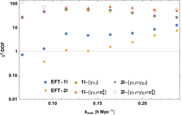
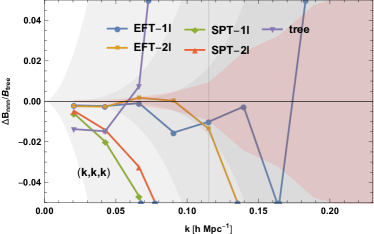
Figure 1: Left: Reduced $\chi^{2}$ for the EFT one- and two-loop bispectra relative to N-body simulation results, for a set of triangles with side lengths up to $k_{\mathrm{max}}$. In addition to the four- and five-parameter models, we show the $\chi^{2}$ for simplified approaches with zero or one parameter (for the zero-parameter models, $\gamma_{1}=c_{s}^{2}$ where $c_{s}^{2}$ is calibrated from the power spectrum). Right: The difference of the perturbative and the N-body result, normalized to the tree-level for a equilateral triangle configuration of side length $k$. The red shaded region indicates uncertainty from the N-body simulations, while the dark gray areas indicate expected theoretical uncertainty at tree-level, one-loop and two-loop, with increasing darkness, respectively.

5 Conclusion

In this work we compute for the first time the two-loop bispectrum of large-scale structure in the EFTofLSS. We derive the analytic double-hard limit of the two-loop correction, showing that this contribution can be exactly absorbed by the four EFT operators known from the one-loop bispectrum. In addition we adopt a simplified treatment for the single-hard region, introducing one extra EFT parameter. We compare our results to N-body simulations, using gridPT in order to beat cosmic variance, and find that adding the two-loop contribution extends the range of wavenumbers with $1\sigma$ agreement from $k\simeq 0.08$ to $0.15\leavevmode\nobreak\ h/\mathrm{Mpc}$.

References

References

- [1] D. Baumann et. al. JCAP 07, 051 (2012).
- [2] J. J. M. Carrasco et. al. JHEP 09, 082 (2012).
- [3] T. Baldauf et. al. JCAP 05, 007 (2015)
- [4] R. Angulo et. al. JCAP 10, 039 (2015)
- [5] T. Baldauf et. al. Phys. Rev. D 104, 12 (2021)
- [6] T. Baldauf et. al. Phys. Rev. D 92, 12 (2015)