Index-zero closed geodesics and stable figure-eights in convex hypersurfaces

Abstract

For each odd $n\geq 3$, we construct a closed convex hypersurface of $\mathbb{R}^{n+1}$ that contains a non-degenerate closed geodesic with Morse index zero. A classical theorem of J. L. Synge would forbid such constructions for even $n$, so in a sense we prove that Synge’s theorem is ”sharp.” We also construct stable figure-eights: that is, for each $n\geq 3$ we embed the figure-eight graph in a closed convex hypersurface of $\mathbb{R}^{n+1}$, such that sufficiently small variations of the embedding either preserve its image or must increase its length.

These index-zero geodesics and stable figure-eights are mainly derived by constructing explicit billiard trajectories with “controlled parallel transport” in convex polytopes.

2020 Mathematics Subject Classification. Primary 53C22; Secondary 53C42

1 Introduction

Can one lasso a convex body? Or, more formally, can a convex hypersurface of Euclidean space contain a non-degenerate closed geodesic with Morse index zero? The answer will depend on the parity of the dimension of the hypersurface. In this paper we construct non-degenerate closed geodesics with Morse index zero in certain convex hypersurfaces, as well as stable geodesic nets, which generalize those closed geodesics. Roughly speaking, a stable geodesic net in a Riemannian manifold $M$ is an immersion in $M$ of a connected graph $\Gamma$, so that every edge is immersed as a constant-speed geodesic and every sufficiently small perturbation of the immersion either preserves its image or increases its length. This means that among the space of immersions of $\Gamma$ in a given manifold, a stable geodesic bouquet is a local minimum under the length functional. Stable geodesic bouquets are special cases of stationary geodesic nets, which are stationary points in the space of immersions of a given connected graph $\Gamma$ [Pit74, AA76, NR07, Rot11, LS21, HM96]. Stationary geodesic nets and stable geodesic bouquets are formally defined in [Che22, Section 2]. In this paper we will mainly construct non-degenerate closed geodesics with index zero (which are precisely the stable geodesic bouquets with one loop), as well as stable geodesic nets that are immersions of the figure-eight graph, which we call stable figure-eights.

We will mostly consider stable geodesic nets that are immersions of “flower-shaped” graphs $\mathcal{B}_{k}$ comprising $k\geq 1$ loops at a single vertex. Such nets are called stable geodesic bouquets.

Index-zero closed geodesics and stable geodesic nets are easier to construct in manifolds $M$ that are not simply-connected or have some negative curvature. If $M$ is not simply-connected, then continuously contracting any closed loop that is not null-homotopic would eventually yield an index-zero closed geodesic. Similarly, if we have $k$ loops based at the same point $p\in M$ that represent non-trivial elements in $\pi_{1}(M,p)$, then we could construct a stable geodesic bouquet by gluing every loop at the basepoint to give an immersion $G:\mathcal{B}_{k}\to M$, and then applying a length-shortening process that perserves the graph structure. Generically, this ensemble of loops should converge to a stable geodesic bouquet.

Even when $M$ is simply-connected, if it has a closed geodesic in a region with strictly negative curvature, then it must have index zero due to the formula for the second variation of length. Likewise, if a stationary geodesic net—an immersion of a fixed connected graph that is a critical point under the length functional—lies in a region of strictly negative curvature then it must also be stable.

On the other hand, there are several negative results that rule out the existence of index-zero closed geodesics and stable geodesic bouquets in certain closed manifolds $M$ that are simply-connected and have positive sectional curvature. Indeed, if $M$ is also even-dimensional and orientable, then a classical theorem of J. L. Synge prevents it from having an index-zero closed geodesic [Syn36]. Moreover, a well-known conjecture of H. B. Lawson and J. Simons [LJS73] would imply that if $M$ is closed and simply-connected, and its curvature is $1/4$-pinched, then it cannot contain any stable submanifolds or stable varifolds of any dimension, which includes index-zero closed geodesics and stable geodesic bouquets. This conjecture has been proven under various additional pinching assumptions [How85, SX00, HW03]. In particular, the conjecture holds for all round spheres, so that none of them contain any index-zero closed geodesic or stable geodesic bouquet. I. Adelstein and F. V. Pallete also proved that positively curved Riemannian 2-spheres cannot have a stable geodesic net in the shape of a $\theta$ graph [AP20].

Given these negative results, it is natural to ask which, if any, simply-connected and closed manifolds with positive sectional curvature can contain index-zero closed geodesics or stable geodesic bouquets. Constructions of such manifolds are rarer than the negative results. W. Ziller constructed a 3-dimensional positively-curved homogeneous space that contains an index-zero closed geodesic [Zil76, Example 1]. In addition, the author recently constructed, in every dimension $n\geq 2$, a Riemannian $n$-sphere which is isometric to a convex hypersurface and which contains a stable geodesic bouquet. The bouquet has 3 loops if $n=2$, and has $n$ loops if $n\geq 3$ [Che22]. The convex hypersurfaces have strictly positive sectional curvature. Those stable geodesic bouquets are also irreducible, in the sense that no pair of tangent vectors at the basepoint are parallel. (This rules out “degenerate” stable geodesic bouquets that are merely unions of index-zero closed geodesics. Indeed, many proofs of the existence of stationary geodesic nets that rely on min-max methods are unable to tell whether the result is a union of closed geodesics [NR07, Rot11, LS21].) To our understanding, that was the first existence result for irreducible stable geodesic nets in simply-connected and closed manifolds with strictly positive sectional curvature. In this paper we prove another existence result along the same lines, except that only two loops are necessary in the stable geodesic bouquet:

Theorem 1.1 (Main result).

For every integer $n\geq 3$, there exists a closed convex hypersurface $M_{n}$ of $\mathbb{R}^{n+1}$ with positive sectional curvature that contains a simple, irreducible and stable figure-eight.

Furthermore, for each $n\geq 3$, every Riemannian $n$-sphere whose metric is sufficiently close to that of $M_{n}$ in the $C^{\infty}$ topology also contains a simple, irreducible and stable figure-eight.

(By simple we mean that the stable figure-eight is an injective immersion. Note that no stable figure-eight in a Riemannian surface (i.e. $n=2$) can be irreducible.)

On the face of it, this result seems stronger than the one in [Che22] in the sense that when we are allowed to have more loops, it seems easier to “arrange” the loops into a stable geodesic bouquet. Using only two geodesic loops $\gamma_{1},\gamma_{2}:I\to M$ gives us much less freedom, because the condition of being a critical point of the length functional requires that the same line must bisect the angle between $\gamma_{1}^{\prime}(0)$ and $-\gamma_{1}^{\prime}(1)$ as well as the angle between $\gamma_{2}^{\prime}(0)$ and $-\gamma_{2}^{\prime}(1)$. Moreover, both of those angles must be equal in magnitude.

Nevertheless, our main result is independent from the one in [Che22]. We will explain how using only two loops forces us to control the parallel transport map along the geodesic loops more precisely. The new techniques developed in this paper for such precise control will also yield “elementary” constructions of index-zero closed geodesics in convex hypersurfaces, which in some sense proves that the aforementioned theorem of Synge is “sharp”:

Theorem 1.2.

For every odd integer $n\geq 3$, there exists a closed convex hypersurface $M_{n}^{\prime}$ of $\mathbb{R}^{n+1}$ with positive sectional curvature that contains a simple closed geodesic with index zero.

Furthermore, for each odd $n\geq 3$, every Riemannian $n$-sphere whose metric is sufficiently close to that of $M_{n}^{\prime}$ in the $C^{\infty}$ topology also contains a simple closed geodesic with index zero.

(Simple means that the closed geodesic does not self-intersect.)

It may be possible that Ziller’s construction can be generalized to find index-zero closed geodesics in positively-curved homogeneous spaces of higher odd dimension. However, these spaces could never be isometric to closed convex hypersurfaces of Euclidean space; if that were possible, then they would have to be isometric to a round sphere due to a result by S. Kobayashi [Kob58]. The existence of an index-zero closed geodesic in this round sphere would then contradict a special case of the conjecture by Lawson and Simons which has been proven, for instance, by R. Howard [How85].

We also point out that the index-zero closed geodesics and stable figure-eights that we construct can be considered as “elementary” because they essentially lie in manifolds with flat Riemannian metric away from some singularities (which we eventually smooth into convex hypersurfaces), and also because the geodesics involved are derived from certain billiard trajectories in convex polytopes that can be explicitly computed.

1.1 Motivation for the key ideas

1.1.1 Index-zero closed geodesics as core curves of maximally-twisted tubes

The connection between stability and parallel transport can be appreciated more immediately in the simplest case of a simple closed geodesic $\gamma:I\to M$ based at the point $p=\gamma(0)=\gamma(1)$ in an orientable manifold $M$. Consider the “component of the parallel transport map along $\gamma$ that is orthogonal to $\gamma^{\prime}$,” that is, the map $P^{\perp}:T_{p}M^{\perp}\to T_{p}M^{\perp}$ that is the restriction of the parallel transport map to the subspace $T_{p}M^{\perp}\subset T_{p}M$ of vectors orthogonal to $\gamma^{\prime}(0)=\gamma^{\prime}(1)$. Synge defined the “twist” of $\gamma$ to be the smallest value of $\cos^{-1}\left\langle P^{\perp}u,u\right\rangle$ for all unit vectors $u\in T_{p}M^{\perp}$. He then proved that if $M$ has curvature bounded from below by a constant $K_{0}>0$ and $\gamma$ has index zero, then the twist of $\gamma$ must be at least $\operatorname{length}(\gamma)\sqrt{K_{0}}$ (see Theorem II in [Syn36]).

This suggests a rule of thumb: to construct a simple closed geodesic that is stable, construct it so that its tubular neighbourhood is “sufficiently twisted.” This leads us to some concrete examples that will form the basis of our proof of Theorem 1.2, namely the index-zero closed geodesics that are the core curves of1 “maximally-twisted tubes.” More precisely, for some integer $n\geq 2$ and lengths $r,\ell>0$, consider the space $(\mathbb{D}^{n-1}_{r}\times[0,\ell])/{\sim}$, where $\mathbb{D}^{n-1}_{r}$ is the closed disk of radius $r$ centered at the origin in $\mathbb{R}^{n-1}$, and the equivalence relation $\sim$ identifies $(x,0)$ with $(-x,\ell)$ for all $x\in\mathbb{D}^{n-1}_{r}$. The resulting space is a “tube” $T$ with a flat Riemannian metric, which we call an $n$-dimensional maximally-twisted tube. (When $n=2$ this is a Möbius strip.) $T$ is orientable if and only if $n$ is odd. Parallel transport along the core curve $\gamma:[0,\ell]\to T$ satisfies $P^{\perp}(v)=-v$, so $\gamma$ has twist equal to the maximum possible value of $\pi$. An elementary argument shows that $\gamma$ attains the minimal length among all smooth closed curves in $T$ freely homotopic to $\gamma$. Alternatively, one can see that $\gamma$ must have index zero because $T$ has a flat Riemannian metric, so the curvature term in the second variation of length vanishes, which forces the second variation to always be non-negative. We will prove that $\gamma$ is non-degenerate later in Lemma 3.1.

Maximally-twisted tubes will help us prove Theorem 1.2 in the following way. For each odd $n\geq 3$ we will first embed an $n$-dimensional maximally-twisted tube in a “polyhedral manifold” obtained by gluing two copies of a convex $n$-dimensional polytope $\mathbf{X}^{n}\subset\mathbb{R}^{n}$ (henceforth, $n$-polytope) along their boundaries via the identity map. The result, called the double of $\mathbf{X}^{n}$ and denoted by $\mathcal{D}_{\mathrm{}}\mathbf{X}^{n}$, is a topological manifold homeomorphic to the $n$-sphere. In fact, $\mathcal{D}_{\mathrm{}}\mathbf{X}^{n}$ is a Riemannian manifold with singularities at the image of the $(n-2)$-skeleton of $\mathbf{X}^{n}$. The smooth part of $\mathcal{D}_{\mathrm{}}\mathbf{X}$ is the complement of its singularities, denoted by $\mathcal{D}_{\mathrm{sm}}\mathbf{X}^{n}$, which has a flat Riemannian metric induced from the Euclidean metric on $\mathbf{X}^{n}$. The maximally-twisted tube will be isometrically embedded in $\mathcal{D}_{\mathrm{sm}}\mathbf{X}^{n}$, and its core curve will be an index-zero closed geodesic $\gamma_{n}$. The final step will then be to smooth $\mathcal{D}_{\mathrm{}}\mathbf{X}^{n}$ into a convex hypersurface in $\mathbb{R}^{n+1}$ while preserving the stability of $\gamma_{n}$, using arguments from [Che22, Appendices B and C]. Here it is important that $\gamma_{n}$ is non-degenerate, to ensure that after sufficiently small changes in the ambient metric from the smoothing, $\gamma_{n}$ will be close to a new index-zero closed geodesic.

$\mathbf{X}^{3}$, $\mathcal{D}_{\mathrm{}}\mathbf{X}^{3}$ and $\gamma_{3}$ are illustrated in Figure 1.1(a)–(b). To illustrate that some tubular neighbourhood of $\gamma_{n}$ is in fact a 3-dimensional maximally-twisted tube—and therefore that $\gamma_{3}$ stable—note that in a maximally-twisted tube $(\mathbb{D}^{2}_{r}\times[0,\ell])/{\sim}$, every line segment $\sigma\subset\mathbb{D}^{2}_{r}$ centered at the origin corresponds to a Mob̈ius strip $(\sigma\times[0,\ell])/{\sim}$. This is the Möbius strip illustrated in Figure 1.1(c)–(d).

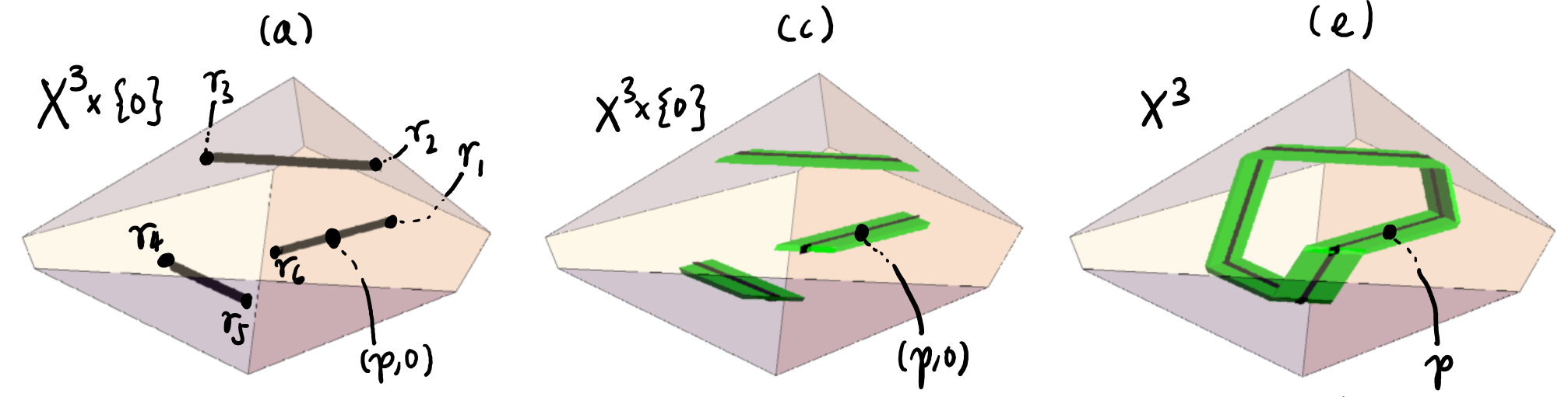
Figure 1.1: Illustration of a polyhedron $\mathbf{X}^{3}$ whose double $\mathcal{D}_{\mathrm{}}\mathbf{X}^{3}$ contains an index-zero closed geodesic $\gamma_{3}$. The two copies of $\mathbf{X}^{3}$ in $\mathcal{D}_{\mathrm{}}\mathbf{X}^{3}$ are depicted in (a) and (b) respectively. The segments of $\gamma_{3}$ in each copy are drawn as thick dark line segments in (a) and (b). $\mathcal{D}_{\mathrm{}}\mathbf{X}^{3}$ contains a Möbius strip $M$ whose core curve is $\gamma_{3}$; the pieces of the Möbius strip in each copy of $\mathbf{X}^{3}$ are drawn in green in (c) and (d). (e) depicts the images of both $\gamma_{3}$ and the Möbius strip $M$ under the canonical quotient map $\mathcal{D}_{\mathrm{}}\mathbf{X}^{3}\to\mathbf{X}^{3}$. (f): $M$ is indeed a Möbius strip because when one attempts to colour it differently on each side of its core curve, the colors will conflict at $p$. The Möbius strip in (e) resembles the origami Möbius strip in (g) that can be folded from paper.

Let us briefly outline the construction of $\mathbf{X}^{3}$ and $\gamma_{3}$ and hint at how it can be generalized to prove all cases of Theorem 1.2. We began with an equilateral triangle $\mathbf{X}^{2}$ and a geodesic $\gamma^{2}:I\to\mathcal{D}_{\mathrm{}}\mathbf{X}^{2}$ that is “almost a periodic geodesic” except that it starts and ends on different copies of $\mathbf{X}^{2}$ in $\mathcal{D}_{\mathrm{}}\mathbf{X}^{2}$. More precisely, its endpoints are different but have the same image under the canonical quotient map $q:\mathcal{D}_{\mathrm{}}\mathbf{X}^{2}\to\mathbf{X}^{2}$ that identifies the two copies of $\mathbf{X}^{2}$ in $\mathcal{D}_{\mathrm{}}\mathbf{X}^{2}$ (see Figure 1.2). This also identifies the tangent spaces at the endpoints of $\gamma^{2}$, and $\gamma^{2}$ is chosen such that under this identification, $(\gamma^{2})^{\prime}(0)$ and $(\gamma^{2})^{\prime}(1)$ are the same. This allows us to treat its parallel transport map $(T_{\gamma(0)}\mathcal{D}_{\mathrm{}}\mathbf{X}^{2})^{\perp}\to(T_{\gamma(1)}\mathcal{D}_{\mathrm{}}\mathbf{X}^{2})^{\perp}$ on the components of tangent spaces orthogonal to $(\gamma^{2})^{\prime}$ as a linear isomorphism on $(T_{\gamma(0)}\mathcal{D}_{\mathrm{}}\mathbf{X}^{2})^{\perp}$, which is in fact $v\mapsto-v$. (Observe the resemblence to the definition of a maximally-twisted tube.) We then use our original constructions called beveling and origami models to convert $\mathbf{X}^{2}$ to $\mathbf{X}^{3}\subset\mathbb{R}^{3}$ and $\gamma^{2}$ to $\gamma^{3}$ in such a way that the projection of $\mathbf{X}^{3}$ onto the first two coordinates is very similar to $\mathbf{X}^{2}$ (this can be observed to some extent by comparing Figures 1.1 and 1.2), and the component of the parallel transport map along $\gamma^{3}$ that is orthogonal to $(\gamma^{3})^{\prime}$ is also $v\mapsto-v$. In other words, the “maximal twist” is preserved from $\gamma^{2}$ to $\gamma^{3}$, which gives rise to the maximally-twisted tube embedded in $\mathcal{D}_{\mathrm{}}\mathbf{X}^{3}$ around $\gamma^{3}$.

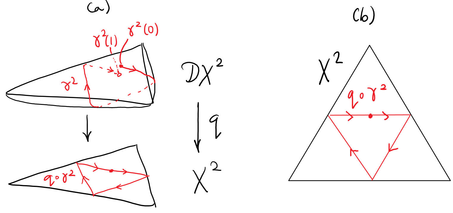
Figure 1.2: (a) The equilateral triangle $\mathbf{X}^{2}$ and the geodesic $\gamma^{2}:I\to\mathcal{D}_{\mathrm{}}\mathbf{X}^{2}$ from which $\mathbf{X}^{3}$ and $\gamma^{3}$ in Figure 1.1 are derived. $q:\mathcal{D}_{\mathrm{}}\mathbf{X}^{2}\to\mathbf{X}^{2}$ is the canonical quotient map. (b) An illustration of $q\circ\gamma^{2}$.

To prove Theorem 1.2, we will apply beveling and origami models to $\mathbf{X}^{3}$ and $\gamma^{3}$ in a similar way to produce a 4-polytope $\mathbf{X}^{4}$ and geodesic $\gamma^{4}:I\to\mathcal{D}_{\mathrm{}}\mathbf{X}^{4}$, and iterate in this way to produce a sequence of $\mathbf{X}^{n}$ and $\gamma^{n}$ for $n\geq 2$. When $n$ is odd $\gamma^{n}$ will be a periodic geodesic, but when $n$ is even $\gamma^{n}$ will be “almost periodic” in the same sense as $\gamma^{2}$. Nevertheless, in any case the component of the parallel transport map along $\gamma^{n}$ that is orthogonal to $(\gamma^{n})^{\prime}$ will always be $v\mapsto-v$. For odd $n\geq 3$ this will give an $n$-dimensional maximally-twisted tube around $\gamma^{n}$ in $\mathcal{D}_{\mathrm{}}\mathbf{X}^{n}$, which will prove most of Theorem 1.2.

1.1.2 Stable figure-eights from “incompatibly-twisted” parallel transport

Our main result in this paper is proven by combining the new techniques of beveling and origami models with earlier tools from [Che22]. Our earlier result in [Che22] was proven by controlling the parallel transport maps along the geodesics in a stable geodesic bouquet. Essentially, given a stationary geodesic bouquet composed of loops $\gamma_{1},\dotsc,\gamma_{k}$ based at a point $p$, we can associate each $\gamma_{i}$ with a vector space $\ker D_{\gamma_{i}}\subset T_{p}M$ such that the stationary geodesic bouquet is stable if $\bigcap_{i=1}^{k}\ker D_{\gamma_{i}}=\{0\}$ and if the sectional curvature along the geodesic bouquet is sufficiently small. Each $\ker D_{\gamma_{i}}$ is defined using the parallel transport map along $\gamma_{i}$, and is called the parallel defect kernel of $\gamma_{i}$. In our construction of stable geodesic bouquets in [Che22], the parallel defect kernels turn out to be hyperplanes of dimension $\dim(M)-1$. Consequently, as $\dim(M)$ increased, we used more and more loops in our geodesic bouquet to guarantee that the intersection of the associated hyperplanes would be a point.

Our main result in this paper will be proven by using beveling and origami models to control parallel transport even more precisely to produce geodesic loops in $M$ whose parallel defect kernels have dimension at most $\dim(M)/2$. This will eventually allow us to construct stable geodesic bouquets using only two loops by “twisting their parallel transport maps in incompatible ways,” resulting in parallel defect kernels that intersect only at the origin. We will carry out the above process for $\dim(M)\in\{3,4,5\}$ in a somewhat ad-hoc fashion in each dimension. Finally, we will combine these low-dimensional examples into examples in all higher dimensions using the following technique.

1.1.3 Combining low-dimensional constructions into high-dimensional ones

If $F$ and $G$ are stable geodesic bouquets with $k$ loops in the doubles of an $m$-polytope $\mathbf{X}_{1}$ and an $n$-polytope $\mathbf{X}_{2}$ respectively, then given a few additional minor assumptions we can combine them into a stable geodesic bouquet in the double of an $(m+n)$-polytope. The idea behind this is most naturally presented through the lens of a certain correspondence between billiard trajectories $\beta$ in $\mathbf{X}$ and geodesics $\gamma$ in $\mathcal{D}_{\mathrm{}}\mathbf{X}$. (A billiard trajectory in $\mathbf{X}$ is a path that travels in a straight line until it collides with the interior of a face of $\mathbf{X}$, after which its velocity vector gets reflected about that face and the trajectory proceeds with the new velocity in another straight line, and so on.) For instance, it is apparent from Figure 1.2 that projecting the geodesic $\gamma^{2}$ via the canonical quotient map $q:\mathcal{D}_{\mathrm{}}\mathbf{X}^{2}\to\mathbf{X}^{2}$ yields a billiard trajectory in $\mathbf{X}^{2}$. In general the correspondence is such that $\gamma$ projects to $\beta$ in the same way, and whenever $\beta$ makes a collision, $\gamma$ passes from one copy of $\mathbf{X}$ in $\mathcal{D}_{\mathrm{}}\mathbf{X}$ to the other. (Note that each billiard trajectory could correspond to two possible geodesics, depending on which copy of $\mathbf{X}$ in $\mathcal{D}_{\mathrm{}}\mathbf{X}$ the geodesic begins from.)

If $\gamma_{i}:[a,b]\to\mathcal{D}_{\mathrm{}}\mathbf{X}_{i}$ are geodesics in the doubles of convex polytopes $\mathbf{X}_{i}$ for $i\in\{1,2\}$, then they correspond to billiard trajectories $\beta_{i}:[a,b]\to\mathbf{X}_{i}$. One can verify that the path $\beta(t)=(\beta_{1}(t),\beta_{2}(t))$ is a billiard trajectory in $\mathbf{X}_{1}\times\mathbf{X}_{2}$, as long as $\beta_{1}$ and $\beta_{2}$ never collide simultaneously. Under that assumption, $\beta$ corresponds to some geodesic in $\mathcal{D}_{\mathrm{}}(\mathbf{X}_{1}\times\mathbf{X}_{2})$. In this manner we can combine the geodesic loops of $F$ and $G$ into geodesic loops in $\mathcal{D}_{\mathrm{}}(\mathbf{X}_{1}\times\mathbf{X}_{2})$, which will form a stationary geodesic bouquet we denote by $F\oplus G$. We will prove that this is stable essentially by proving an inequality that relates the second variations in length of $F$, $G$ and $F\oplus G$.

1.2 Organization of content

In Section 2 we effectively reduce Theorem 1.1 to the cases in dimensions 3, 4, and 5. We accomplish this by explaining how to combine constructions of stable geodesic bouquets in the doubles of low-dimensional polytopes into stable geodesic bouquets in the doubles of polytopes with higher dimension. In particular we prove that stability is preserved in the combination under certain minor conditions.

In Section 3 we define our key constructions of beveling and origami models, prove their key properties, and then use them to construct doubles of polytopes that contain maximally-twisted tubes. This will lead to a proof of Theorem 1.2. Proving the properties of bevelings and origami models will be the most technical part of this paper.

In Section 4, we construct stable figure-eights in the doubles of polytopes with dimensions 3, 4 and 5 using bevelings, origami models and a slight generalization of some ideas from Section 2. Then we combine these constructions into stable figure-eights in polytopes of all higher dimensions using the techniques of Section 2, and complete our proof of our main result.

1.3 Notation and Terminology

We will require that geodesics and billiard trajectories be parametrized at constant speed. We will say that paths $\alpha:[a,b]\to X$ like geodesics or billiard trajectories are simple if they are injective except possibly that $\alpha(a)=\alpha(b)$. We may sometimes write $\alpha$ to denote its image. A stable geodesic bouquet, and more generally any stationary geodesic net, is called simple if it is injective as an immersion. A billiard trajectory $\beta:[a,b]\to\mathbf{X}$ is called a billiard loop if $\beta(a)=\beta(b)$. If it also satisfies $\beta^{\prime}(a)=\beta^{\prime}(b)$, then it is called a periodic billiard trajectory.

When $V:I\to TM$ is a vector field along a geodesic $\gamma:I\to M$, $V(t)^{\perp}$ will refer to the component of $V(t)$ that is orthogonal to $\gamma^{\prime}(t)$. $V^{\perp}$ will refer to the vector field $V^{\perp}(t)=V(t)^{\perp}$.

We will also denote function composition with the symbol $\circ$, but will often omit it when composing linear operators on the same space. If $f:X\to Y$ and $g:X\to Z$ are maps, let $(f,g)$ denote the map $X\to Y\times Z$ that sends $x$ to $(f(x),g(x))$.

Acknowledgements

The author would like to thank his academic advisors Alexander Nabutovsky and Regina Rotman for suggesting this research topic, and for valuable discussions. The author would also like to thank Isabel Beach for useful discussions.

2 Direct Sum of Stationary Geodesic Bouquets

To prove Theorem 1.1, we can begin by constructing, for every integer $n\geq 3$, an $n$-polytope $\mathbf{X}^{n}$ such that $\mathcal{D}_{\mathrm{}}\mathbf{X}^{n}$ contains a simple and irreducible stable figure-eight. After that we can apply the smoothing arguments in [Che22, Appendices B and C] to derive Theorem 1.1. We will reduce the constructions of $\mathbf{X}^{n}$ to the cases where $n\in\{3,4,5\}$. We will do this by showing how to combine a stable geodesic bouquet in the double of an $n_{1}$-polytope with another stable geodesic bouquet in the double of an $n_{2}$-polytope to get a stable geodesic bouquet in the double of an $(n_{1}+n_{2})$-polytope.

Suppose that $F:\mathcal{B}_{k}\to\mathcal{D}_{\mathrm{}}\mathbf{X}$ and $G:\mathcal{B}_{k}\to\mathbf{Y}$ are stationary geodesic bouquets in an $m$-polytope $\mathbf{X}$ and an $n$-polytope $\mathbf{Y}$. respectively. Let the geodesic loops of $F$ and $G$ be $\phi_{1},\dotsc,\phi_{k}:I\to M$ and $\gamma_{1},\dotsc,\gamma_{k}:I\to N$ respectively. Then each geodesic $\phi_{i}$ corresponds to a billiard trajectory $\alpha_{i}$ in $\mathbf{X}$, and similarly each $\gamma_{i}$ corresponds to a billiard trajectory $\beta_{i}$ in $\mathbf{Y}$. As explained in Section 1.1.3, $(\alpha_{i},\beta_{i})$ is a billiard trajectory in $\mathbf{X}\times\mathbf{Y}$ as long as $\alpha_{i}$ and $\beta_{i}$ never collide simultaneously. When this condition folds for all $1\leq i\leq k$, we say that $F$ and $G$ are non-singular and observe that each $(\alpha_{i},\beta_{i})$ corresponds to a geodesic loop in $\mathcal{D}_{\mathrm{}}(\mathbf{X}\times\mathbf{Y})$. We can choose these $k$ geodesic loops to be based at the same point, and one can verify that they combine into a stationary geodesic bouquet which we denote by $F\oplus G$ and call the direct sum of $F$ and $G$.

We aim to prove that whenever $F$ and $G$ are stable, so is $F\oplus G$, provided that $F$ and $G$ are non-singular. To this end, we will consider the index forms of these three stationary geodesic bouquets: quadratic forms $Q_{F}(-)$, $Q_{G}(-)$ and $Q_{F\oplus G}(-)$ defined in [Che22, Equation (3.2)]. In particular, we will relate these index forms via an inequality. To prove this inequality it will be convenient to consider an intermediate object: the stationary geodesic bouquet $(F,G)$ in $\mathcal{D}_{\mathrm{}}\mathbf{X}\times\mathcal{D}_{\mathrm{}}\mathbf{Y}$. Then $F\oplus G=\Gamma\circ(F,G)$, where $\Gamma$ is a branched cover defined as follows:

$$\begin{gathered}\Gamma:\mathcal{D}_{\mathrm{}}\mathbf{X}\times\mathcal{D}_{\mathrm{}}\mathbf{Y}\to\mathcal{D}_{\mathrm{}}(\mathbf{X}\times\mathbf{Y})\\ \Gamma((x,\xi_{1}),(y,\xi_{2}))=((x,y),\xi_{1}+\xi_{2}\bmod 2).\end{gathered}$$ (2.1)

This is a well-defined continuous map, and in fact is a 2-sheeted branched covering whose branch locus is the $(m+n-2)$-skeleton of $\mathcal{D}_{\mathrm{}}\mathbf{X}\times\mathcal{D}_{\mathrm{}}\mathbf{Y}$. ($\mathbf{X}$ has a natural CW structure given by its interior, faces, edges, vertices and so on. This induces a CW structure on $\mathcal{D}_{\mathrm{}}\mathbf{X}$, and eventually on $\mathcal{D}_{\mathrm{}}\mathbf{X}\times\mathcal{D}_{\mathrm{}}\mathbf{Y}$.) Away from the branch locus, $\Gamma$ is a local isometry. As a consequence, $F\oplus G=\Gamma\circ(F,G)$ is stable if and only if $(F,G)$ is stable.

Lemma 2.1 (Superadditivity of index forms).

Let $F$ and $G$ be stationary geodesic bouquets with $k$ loops in Riemannian manifolds $M$ and $N$, and based at $p$ and $q$ respectively. For any vector field $W$ on $(F,G)$, let $W=(U,V)$ where $U$ is the component of $W$ in $TM$ and $V$ is the component in $TN$. Then

$$Q_{(F,G)}(W)\geq Q_{F}(U)+Q_{G}(V).$$ (2.2)

Proof.

Let the geodesic loops of $F$ and $G$ be $\phi_{1},\dotsc,\phi_{k}:I\to M$ and $\gamma_{1},\dotsc,\gamma_{k}:I\to N$ respectively. Let $\eta_{i}=(\phi_{i},\gamma_{i})$. First we will prove that for any vector field $W_{i}=(U_{i},V_{i})$ along $\eta_{i}$ (that may not agree at the basepoint $(p,q)$), $Q_{\eta_{i}}(W_{i})=Q_{\phi_{i}}(U_{i})+Q_{\gamma_{i}}(V_{i})$.

Let $\nabla^{M}$ and $\nabla^{N}$ denote the Riemannian connections on $M$ and $N$ respectively. Then

$$Q_{\eta_{i}}(W_{i}) =\int_{0}^{1}\left\lVert\nabla_{\eta_{i}^{\prime}(t)}W_{i}\right\rVert^{2}\,dt$$ (2.3)

$$=\int_{0}^{1}\left\lVert\left(\nabla^{M}_{\phi_{i}^{\prime}(t)}U_{i},\nabla^{N}_{\gamma_{i}^{\prime}(t)}V_{i}\right)\right\rVert^{2}\,dt$$ (2.4)

$$=\int_{0}^{1}\left\lVert\nabla^{M}_{\phi_{i}^{\prime}(t)}U_{i}\right\rVert^{2}\,dt+\int_{0}^{1}\left\lVert\nabla^{N}_{\gamma_{i}^{\prime}(t)}V_{i}\right\rVert^{2}\,dt$$ (2.5)

$$=Q_{\phi_{i}}(U_{i})+Q_{\gamma_{i}}(V_{i}).$$ (2.6)

Consider some $1\leq i\leq k$. Let $m=\dim(M)$, and let $X_{1},\dotsc,X_{m-1},X_{m}=\phi_{i}^{\prime}/\left\lVert\phi_{i}^{\prime}\right\rVert$ be a parallel orthonormal frame along $\phi_{i}$. Let $U_{i}=\sum_{j=1}^{m}a_{j}X_{j}$ for smooth functions $a_{j}:I\to\mathbb{R}$. Then

$$Q_{\phi_{i}}(U_{i}) =\int_{0}^{1}\left\lVert\nabla^{M}_{\phi_{i}^{\prime}(t)}U_{i}\right\rVert^{2}\,dt$$ (2.7)

$$=\int_{0}^{1}\left\lVert\nabla^{M}_{\phi_{i}^{\prime}(t)}\sum_{j=1}^{m}a_{j}(t)X_{j}(t)\right\rVert^{2}\,dt$$ (2.8)

$$=\int_{0}^{1}\sum_{j=1}^{m}a_{j}^{\prime}(t)^{2}\,dt$$ (2.9)

$$\geq\int_{0}^{1}\sum_{j=1}^{m-1}a_{j}^{\prime}(t)^{2}\,dt$$ (2.10)

$$=Q_{\phi_{i}}\left(\sum_{j=1}^{m-1}a_{j}X_{j}\right).$$ (2.11)

Therefore $Q_{\phi_{i}}(U_{i})$ does not increase when its argument is replaced with the component that is orthogonal to $\phi_{i}$. The same conclusion on $Q_{\gamma_{i}}(V_{i})$ follows from a similar computation involving a parallel orthonormal frame $Y_{1},\dotsc,Y_{n-1},Y_{n}=\gamma_{i}^{\prime}/\left\lVert\gamma_{i}^{\prime}\right\rVert$, where $n=\dim(N)$.

Let $(\tilde{U}_{i},\tilde{V}_{i})$ be the component of $W_{i}$ orthogonal to $\eta_{i}$. This is obtained by adding or subtracting some multiple of $(\phi_{i}^{\prime},\gamma_{i}^{\prime})=(\left\lVert\phi_{i}^{\prime}\right\rVert X_{m},\left\lVert\gamma_{i}^{\prime}\right\rVert Y_{n})$ from $W_{i}$. This implies that $U_{i}$ and $\tilde{U}_{i}$ have the same component $U_{i}^{\perp}$ that is orthogonal to $\phi_{i}$, and similarly $V_{i}$ and $\tilde{V}_{i}$ have the same component $V_{i}^{\perp}$ that is orthogonal to $\gamma_{i}$. Therefore

$$Q_{\eta_{i}}\Big{(}(\tilde{U}_{i},\tilde{V}_{i})\Big{)}=Q_{\phi_{i}}(\tilde{U}_{i})+Q_{\gamma_{i}}(\tilde{V}_{i})\geq Q_{\phi_{i}}(U_{i}^{\perp})+Q_{\gamma_{i}}(V_{i}^{\perp}).$$ (2.12)

However this implies that if $W_{i}$ is the restriction of $W$ to $\eta_{i}$, then

$$Q_{(F,G)}(W)=\sum_{i=1}^{k}Q_{\eta_{i}}\Big{(}(\tilde{U}_{i},\tilde{V}_{i})\Big{)}\geq\sum_{i=1}^{k}\Big{(}Q_{\phi_{i}}(U_{i}^{\perp})+Q_{\gamma_{i}}(V_{i}^{\perp})\Big{)}=Q_{F}(U)+Q_{G}(V).$$ (2.13)

∎

The preceding lemma allows us to verify that if $F:\mathcal{B}_{k}\to\mathcal{D}_{\mathrm{}}\mathbf{X}$ and $G:\mathcal{B}_{k}\to\mathcal{D}_{\mathrm{}}\mathbf{Y}$ are stable geodesic bouquets for $m$-polytope $\mathbf{X}$ and $n$-polytope $\mathbf{Y}$, then $(F,G)$ is a stable geodesic bouquet in $\mathcal{D}_{\mathrm{}}\mathbf{X}\times\mathcal{D}_{\mathrm{}}\mathbf{Y}$.

Thus we can derive the following:

Corollary 2.2.

If $F$ and $G$ are stable geodesic bouquets in the doubles of convex polytopes and $F$ and $G$ are non-singular, then $F\oplus G$ is also stable.

Proof.

It suffices to show that $(F,G)$ is stable, which by [Che22, Lemma 3.1] is equivalent to showing that $Q_{(F,G)}(W)=0$ only if the vector field $W$ is tangent to $(F,G)$. Indeed, if $Q_{(F,G)}(W)=0$ then by Lemma 2.1, $Q_{F}(U)=Q_{G}(V)=0$ where $U$ (resp. $V$) is the component of $W$ in $T\mathcal{D}_{\mathrm{sm}}\mathbf{X}$ (resp. $T\mathcal{D}_{\mathrm{sm}}\mathbf{Y}$). Since $F$ is stable, [Che22, Lemma 3.1] implies that $U$ is tangent to $F$. Similarly, $V$ must be tangent to $G$. This implies that $W$ is tangent to $(F,G)$. ∎

We also have the following condition for the direct sum to be simple:

Lemma 2.3.

If $q\circ F$ is injective, where $q:\mathcal{D}_{\mathrm{}}\mathbf{X}\to\mathbf{X}$ is the canonical quotient map, then $F\oplus G$ is simple.

Proof.

Let the geodesic loops of $F$ be $\phi_{1},\dotsc,\phi_{k}$ and let those of $G$ be $\gamma_{1},\dotsc,\gamma_{k}$. By the hypotheses of the lemma, the billiard trajectories $\alpha_{i}$ in $\mathbf{X}$ corresponding to $\phi_{i}$ are all simple loops. Let each $\gamma_{i}$ correspond to a billiard trajectory $\beta_{i}$ in $\mathbf{Y}$. From the definition of direct sum we can see that as explained in Section 1.1.3, the geodesic loops of $F\oplus G$ correspond to billiard trajectories $(\alpha_{i},\beta_{i})$ in $\mathbf{X}\times\mathbf{Y}$, for $1\leq i\leq k$. The hypotheses of the lemma further imply that the billiard trajectories $(\alpha_{i},\beta_{i})$ are simple and intersect each other only at the basepoint. Therefore $F\oplus G$ also has to be simple. ∎

Remark 2.4.

Say that two stationary geodesic bouquets $F:\mathcal{B}_{k}\to\mathcal{D}_{\mathrm{}}\mathbf{X}$ and $G:\mathcal{B}_{k}\to\mathcal{D}_{\mathrm{}}\mathbf{Y}$ are equivalent if $G$ can be obtained from $F$ by post-composing with an isometry $\mathcal{D}_{\mathrm{}}\mathbf{X}\to\mathcal{D}_{\mathrm{}}\mathbf{Y}$. It can easily be verified that $\oplus$ is commutative and associative, up to equivalence. Hence we will slightly abuse notation and treat it as an associative operation. This situation can be summarized by saying that the set $\mathcal{S}_{k}$ of equivalence classes of stationary geodesic bouquets with $k$ loops in doubles of convex polytopes forms a commutative semigroup under the $\oplus$ operation. Moreover, the stable figure-eights in $\mathcal{S}_{k}$ form a subsemigroup, and the irreducible and stable figure-eights in $\mathcal{S}_{k}$ form an ideal. These arguments have been stated for geodesic bouquets for convenience, but they extend to stable geodesic nets that are modeled on any graph.

As explained at the beginning of this section, this operation nearly allows us to reduce Theorem 1.1 to the cases where $n\in\{3,4,5\}$. If there are corresponding $n$-polytopes $\mathbf{X}^{n}$ and simple, irreducible and stable figure-eights $G^{n}:\mathcal{B}_{2}\to\mathcal{D}_{\mathrm{}}\mathbf{X}^{n}$, for $n\in\{3,4,5\}$, then the stable figure-eights of the form

$$G^{3m+n}=G^{n}\oplus G^{3}_{1}\oplus\dotsb\oplus G^{3}_{m}\text{ for }n\in\{3,4,5\},m\geq 0,$$ (2.14)

are also irreducible, where the $G^{3}_{i}$’s are slight modifications of $G^{3}$ to ensure that the direct summands are pairwise non-singular. In Section 4 we will construct $G^{3}$, $G^{4}$ and $G^{5}$ such that all of those stable figure-eights $G^{3m+n}$ will also be simple.

3 Index-zero Closed Geodesics from Bevelings and
Origami Models

The main purpose of this section is to introduce our constructions of bevelings and origami models that allow us to derive, from a billiard trajectory $\beta$ in an $n$-polytope, a billiard trajectory $\hat{\beta}$ in an $(n+1)$-polytope such that the “parallel transport along $\hat{\beta}$” (to be defined later) is controlled in terms of the “parallel transport along $\beta$.” As a result we will also prove Theorem 1.2.

As explained in Section 1.1.1, to prove Theorem 1.2, for each odd $n\geq 3$, we will find an $n$-polytope $\mathbf{X}^{n}$ such that $\mathcal{D}_{\mathrm{sm}}\mathbf{X}^{n}$ contains an isometrically embedded $n$-dimensional maximally twisted tube. It was explained that the core curve $\gamma_{n}:[a,b]\to\mathcal{D}_{\mathrm{}}\mathbf{X}^{n}$ will be an index-zero closed geodesic. Let us prove that it will also be non-degenerate.

Lemma 3.1.

Core curves of maximally-twisted tubes are non-degenerate closed geodesics.

Proof.

Let $\gamma:[0,\ell]\to T$ be the core curve, parametrized by arc-length, of an $n$-dimensional maximally-twisted tube $T$. That is, we have to show that any variation along $\gamma$ (a vector field $V(t)$ such that $V(0)=V(\ell)$) gives a vanishing second variation of length only when $V(t)$ is always parallel to $\gamma^{\prime}(t)$. Let $V(t)=a_{1}(t)E_{1}(t)+\dotsb+a_{n-1}(t)E_{n-1}(t)+a_{n}(t)\gamma^{\prime}(t)$ for some parallel orthonormal frame $E_{1},\dotsc,E_{n-1},\gamma^{\prime}$ and smooth functions $a_{i}$. The definition of a maximally-twisted tube $T=\mathbb{D}_{r}^{n-1}\times[0,\ell]/{\sim}$ implies that we can choose each $E_{i}(s)$ to be tangent to the image of $\mathbb{D}_{r}^{n-1}\times\{s\}$ in $T$ and such that $E_{i}(s)$ corresponds to the $i^{\text{th}}$ standard basis vector of $\mathbb{R}^{n-1}$ in each copy of $\mathbb{D}_{r}^{n-1}$. Thus $E_{i}(\ell)=-E_{i}(0)$.

Suppose that the second variation of length along $V$ vanishes; we will show that the functions $a_{i}$ vanish identically for $1\leq i\leq n-1$. We apply the formula for the second variation in length, noting that it only involves the component of $V$ orthogonal to $\gamma$, and that the curvature term vanishes because $T$ has a flat metric.

$$0=\int_{0}^{\ell}\left\lVert\nabla_{\gamma^{\prime}}\left(\sum_{i=1}^{n-1}a_{i}(t)E_{i}(t)\right)\right\rVert^{2}\,dt=\int_{0}^{\ell}\left\lVert\sum_{i=1}^{n-1}a_{i}^{\prime}(t)E_{i}(t)\right\rVert^{2}\,dt.$$ (3.1)

However, that implies that the functions $a_{1},\dotsc,a_{n-1}$ are all constant. In fact, they must vanish because $V(\ell)=V(0)$ but $E_{i}(\ell)=-E_{i}(0)$. ∎

$\gamma_{n}$ will correspond to some periodic billiard trajectory $\beta_{n}:[a,b]\to\mathbf{X}^{n}$, that will be constructed inductively as follows. We will begin with a certain choice of polygon $\mathbf{X}^{2}\subset\mathbb{R}^{2}$ and periodic billiard trajectory $\beta_{2}:[a,b]\to\mathbf{X}^{2}$. Then for each $n\geq 2$, from the pair of $\mathbf{X}^{n}$ and $\beta_{n}$ we will construct another $(n+1)$-polytope $\mathbf{X}^{n+1}$ that contains a periodic billiard trajectory $\beta_{n+1}$. For odd $n$, $\beta_{n}$ will have an even number of collisions and hence correspond to a closed geodesic $\gamma_{n}$ in $\mathcal{D}_{\mathrm{}}\mathbf{X}^{n}$. A possible set of $\mathbf{X}^{3}$, $\mathcal{D}_{\mathrm{}}\mathbf{X}^{3}$ and $\gamma_{3}$ was illustrated in Figure 1.1.

$\mathbf{X}^{n+1}$ will be constructed in such a way, based on the geometry of $\mathbf{X}^{n}$, such that $\beta_{n+1}$ will be a “folded higher-dimensional version” of $\beta_{n}$. This folding “through the extra dimension” twists the parallel transport map, which enables, for odd $n$, the isometric embedding of maximally-twisted tubes around $\gamma_{n}$.

Outline of this section

Section 3.1 introduces a procedure called beveling for constructing $(n+1)$-polytopes $\mathbf{X}^{n+1}$ out of $n$-polytopes $\mathbf{X}^{n}$. We will see that certain billiard trajectories $\hat{\beta}$ in $\mathbf{X}^{n+1}$ called folded billiard trajectories resemble billiard trajectories $\beta$ in $\mathbf{X}^{n}$ when projected onto the first $n$ coordinates. Section 3.1 will culminate in the proof of a simple relationship between the parallel transport maps of $\hat{\beta}$ and $\beta$ (Lemma 3.6). In Section 3.2 we will prove key properties of folded billiard trajectories. Section 3.3 explains how beveling and folded billiard trajectories can be harnessed to produce the required pair $(\mathbf{X}^{n+1},\beta_{n+1})$ from $(\mathbf{X}^{n},\beta_{n})$. Section 3.4 explains how to derive Theorem 1.2 from those ideas.

3.1 Bevelings

We begin with some notation. Let $\mathbf{X}$ be a convex polytope. Given a billiard trajectory $\beta:[a,b]\to\mathbf{X}$, for all $a\leq s<t\leq b$ such that $\beta(s),\beta(t)\in{\mathbf{X}}^{\circ}$, define the parallel transport map $P_{st}:T_{\beta(s)}\mathbb{R}^{n}\to T_{\beta(t)}\mathbb{R}^{n}$ as $dR_{F_{j}}\dotsm dR_{F_{i}}$, where the collisions between times $s$ and $t$ are at the faces $F_{i},F_{i+1},\dotsc,F_{j}$. Note that this differs from the parallel transport map of a geodesic, but is closely related; see [Che22, Lemma 4.2]. However, in this section we will deal almost exclusively with billiard trajectories instead of geodesics, so by an abuse of notation will write the parallel transport map of billiard trajectories as $P_{st}$.

For each integer $n\geq 1$, let $\operatorname{pr}_{n}:\mathbb{R}^{n+1}\to\mathbb{R}^{n}$ denote the projection onto the first $n$ coordinates. The subscript will be dropped when the dimensions are clear from the context. Let $\Pi_{r}=\mathbb{R}^{n}\times\{r\}$. A subset of $\mathbb{R}^{n}$ is called horizontal if it lies in $\Pi_{r}$ for some $r\in\mathbb{R}$. A path is called horizontal if its image is horizontal. Call the last coordinate of a point $x\in\mathbb{R}^{n}$ its height, denoted by $\operatorname{height}(x)$. If a set is horizontal, its height is the height of any point.

Definition 3.2 (Beveling).

Given an $n$-polytope $\mathbf{X}$, a subset $\mathcal{F}$ of its faces and a function $h:\mathcal{F}\to\mathbb{R}$, a beveling of $\mathbf{X}$ along $\mathcal{F}$ at heights $h$ is an $(n+1)$-polytope $\operatorname{Bev}(\mathbf{X},\mathcal{F},h)$ defined as the intersection of $(n+1)$-polytopes $\mathbf{W}^{h}(F)$ one for each face $F$ of $\mathbf{X}$. The $\mathbf{W}^{h}(F)$ are defined as follows: for each face $F\notin\mathcal{F}$ of $\mathbf{X}$ whose supporting hyperplane is $\mathcal{H}$, let $\mathbf{W}^{h}(F)=\mathcal{H}\times\mathbb{R}$. For each face $F\in\mathcal{F}$, let $\mathbf{W}^{h}(F)$ be the $n$-polytope shaped like a “wedge” that contains $\mathbf{X}\times\{h(F)\}$, and that is bounded by the two hyperplanes that intersect $\mathbf{X}\times\{h(F)\}$ at $F\times\{h(F)\}$, and have a dihedral angle of $\pi/4$ with $\mathbb{R}^{n}\times\{h(F)\}$ (see Figure 3.1(f)). Then $\operatorname{Bev}(\mathbf{X},\mathcal{F},h)=\bigcap_{F}\mathbf{W}^{h}(F)$ where the intersection is taken over all faces of $\mathbf{X}$ (see Figure 3.1(b)).

To simplify our arguments, we will require that for each face $F$ of $\mathbf{X}$, every face of $\mathbf{W}^{h}(F)$ contains a face of $\operatorname{Bev}(\mathbf{X},\mathcal{F},h)$. If $\hat{F}$ is a face of $\operatorname{Bev}(\mathbf{X},\mathcal{F},h)$ that is contained in $\partial\mathbf{W}^{h}(F)$, then we say that $\hat{F}$ is inherited from $\mathbf{W}^{h}(F)$.

Figure 3.1 illustrates an example of a beveling $\hat{\mathbf{X}}=\operatorname{Bev}(\mathbf{X},\mathcal{F},h)$, where $\mathbf{X}\subset\mathbb{R}^{2}$ is an equilateral triangle.

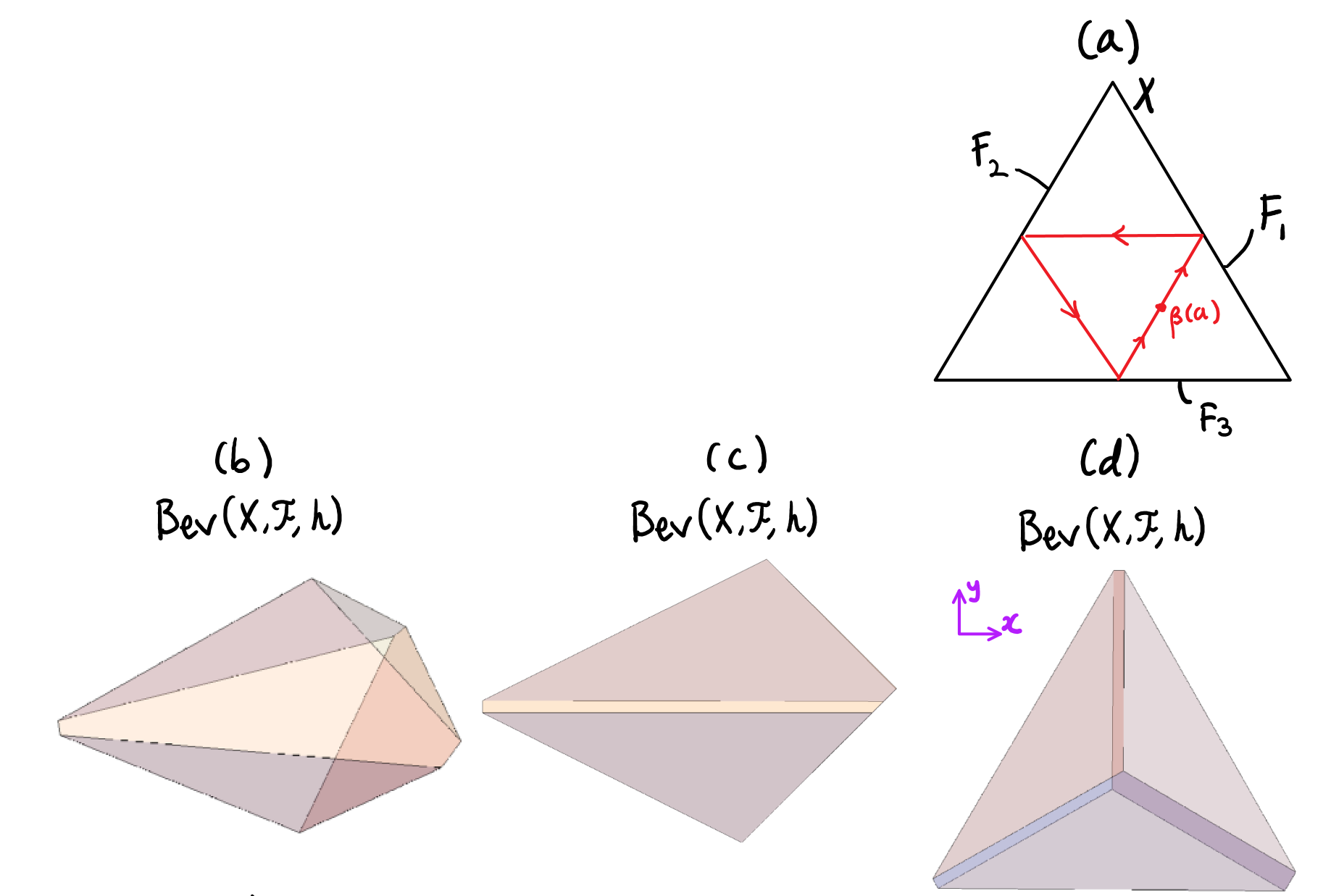
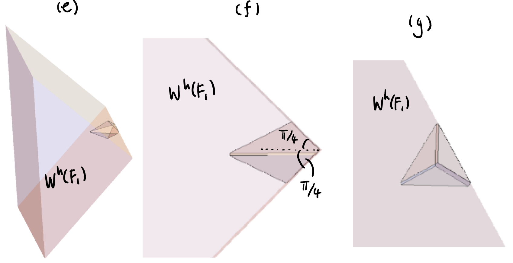
Figure 3.1: An example of a convex 2-polytope (polygon) $\mathbf{X}$ and a beveling $\operatorname{Bev}(\mathbf{X},\mathcal{F},h)$ of it. (a) $\mathbf{X}$ is an equilateral triangle with edge length 2 and “faces” (i.e. edges) $F_{1}$, $F_{2}$ and $F_{3}$. (b), (c), (d): three different views of $\operatorname{Bev}(\mathbf{X},\mathcal{F},h)$, where $\mathcal{F}=\{F_{1},F_{2},F_{3}\}$ and $h(F_{1})=0.05$, $h(F_{2})=0$, and $h(F_{3})=-0.05$. (e), (f), (g): Three different views of $\mathbf{W}^{h}(F_{1})$. In (f), the dashed line represents $\mathbb{R}^{2}\times h(F_{1})$.

If a billiard trajectory $\beta:[a,b]\to\mathbf{X}$ has collisions at times $t_{1},t_{2},\dotsc,t_{k}$ where $a<t_{1}<\dotsb<t_{k}<b$, then the linear paths $\beta|_{[a,t_{1}]},\beta|_{[t_{1},t_{2}]},\dotsc,\beta|_{[t_{k-1},t_{k}]},\beta|_{[t_{k},b]}$ are called the segments of $\beta$.

Definition 3.3 (Folded billiard trajectories, crease-like segments, simulating colliding, simulating folding).

Given a beveling $\operatorname{Bev}(\mathbf{X},\mathcal{F},h)$ of $\mathbf{X}$, we say that a billiard trajectory $\hat{\beta}:[a,b]\to\operatorname{Bev}(\mathbf{X},\mathcal{F},h)$ is folded if $\hat{\beta}(a)$ lies in the interior of $\mathbf{X}$, the first segment of $\hat{\beta}$ is horizontal, and whenever $\hat{\beta}$ collides with a face inherited from $\mathbf{W}^{h}(F)$ for some $F\in\mathcal{F}$, the next face it collides with—if any—is another face inherited from $\mathbf{W}^{h}(F)$. If $\hat{\beta}$ is folded, then we say it simulates colliding at $F_{1},\dotsc,F_{k}$ if it collides with all of the face(s) inherited from $\mathbf{W}^{h}(F_{1})$, followed by all of the face(s) inherited $\mathbf{W}^{h}(F_{2})$, and so on until it collides with at least one face inherited from $\mathbf{W}^{h}(F_{k})$.

We will say that a segment of $\hat{\beta}$ is crease-like if it begins at a point in the interior of a face of $\operatorname{Bev}(\mathbf{X},\mathcal{F},h)$ that is inherited from $\mathbf{W}^{h}(F)$ for some $F\in\mathcal{F}$, and the segment extends into a straight line that intersects the other face of $\mathbf{W}^{h}(F)$ (possibly at a point outside of $\operatorname{Bev}(\mathbf{X},\mathcal{F},h)$). In this case we say that the segment simulates folding around $F$. In the same vein, we will say that $\hat{\beta}$ simulates folding around $F_{1}^{\prime},F_{2}^{\prime},\dotsc,F_{j}^{\prime}$ if its crease-like segments simulate creases at those faces in that order.

In our applications of folded billiard trajectories $\hat{\beta}$, they will be characterized by their behaviour near the boundary of $\operatorname{Bev}(\mathbf{X},\mathcal{F},h)$. In particular, $\hat{\beta}$ can have two main types of behaviour near the boundary of $\mathbf{W}^{h}(F)$, depending on whether $F\in\mathcal{F}$, as illustrated in Figure 3.2. The projection of $\hat{\beta}$ via $\operatorname{pr}$ is also illustrated. If $F\in\mathcal{F}$, then near $\partial\mathbf{W}^{h}(F)$, $\hat{\beta}$ will contain a crease-like segment $\sigma$ that spans between the two faces of $\partial\mathbf{W}^{h}(F)$ as depicted in Figure 3.2(a). The segments before and after $\sigma$ will be horizontal. On the other hand, if $F\in\mathcal{F}$, then near $\partial\mathbf{W}^{h}(F)$, $\hat{\beta}$ will consist of two horizontal segments as depicted in Figure 3.2(b). These statements will be formally proven in Section 3.2.

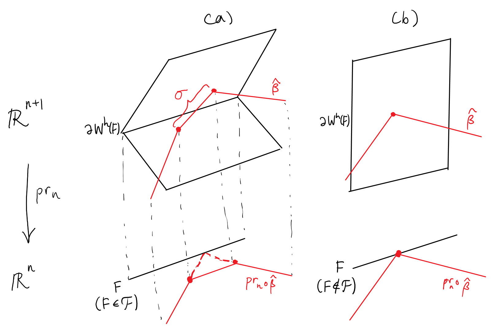
Figure 3.2: The two main types of behaviour that folded billiard trajectories can have near the boundary of a beveling $\operatorname{Bev}(\mathbf{X},\mathcal{F},h)$.

(The definition of folded billiard trajectories may allow for behaviour that looks more complicated than shown in Figure 3.2, but we will choose $\mathbf{X}$ and the beveling $\operatorname{Bev}(\mathbf{X},\mathcal{F},h)$ carefully to keep the behaviour of folded billiard trajectories within these two simple cases.)

Here we provide some motivation for the preceding definitions. In the upper half of Figure 3.2(b), $\hat{\beta}$ is simulating colliding with $F$; this terminology is justified by the phenomenon that $\operatorname{pr}\circ\hat{\beta}$ actually looks like a billiard trajectory in $\mathbf{X}$ that collides with $F$, as shown in the lower half of Figure 3.2(b). A similar situation occurs in Figure 3.2(a) as well, where in the upper half $\hat{\beta}$ is simulating colliding with $F$. However, this time ${\operatorname{pr}}\circ\hat{\beta}$ only looks like a billiard trajectory in $\mathbf{X}$ after extending two of the segments along dashed red lines, as shown in the lower half. The resemblence between ${\operatorname{pr}}\circ\hat{\beta}$ and a billiard trajectory in $\mathbf{X}$ will be formally proven later in Proposition 3.8. In fact, we will prove in Lemma 3.6 that if $\hat{\beta}$ simulates colliding with $F_{1},\dotsc,F_{k}$ and $\beta$ is a billiard trajectory in $\mathbf{X}$ that collides with $F_{1},\dotsc,F_{k}$, then the parallel transport maps of $\beta$ and $\hat{\beta}$ are closely related. This will help us derive $\beta^{n+1}$ from $\beta^{n}$ in a way that controls the parallel transport map, as explained at the beginning of this section.

As a concrete example, Figure 3.3(a)–(c) illustrates a folded billiard trajectory $\hat{\beta}:[a,b]\to\hat{\mathbf{X}}$ that begins at the point $\hat{\beta}(a)$, then passes through the points $x_{1},x_{2},\dotsc,x_{6}$ in that order before returning to $\hat{\beta}(b)=\hat{\beta}(a)$. The crease-like segments of $\hat{\beta}$ are $x_{1}x_{2}$, $x_{3}x_{4}$ and $x_{5}x_{6}$, which simulate folding around $F_{1}$, $F_{2}$ and $F_{3}$ respectively. In this case, $\hat{\beta}$ happens to be periodic with an even number of reflections, so it corresponds to a closed geodesic $\hat{\gamma}$ in $\mathcal{D}_{\mathrm{}}\hat{\mathbf{X}}$.

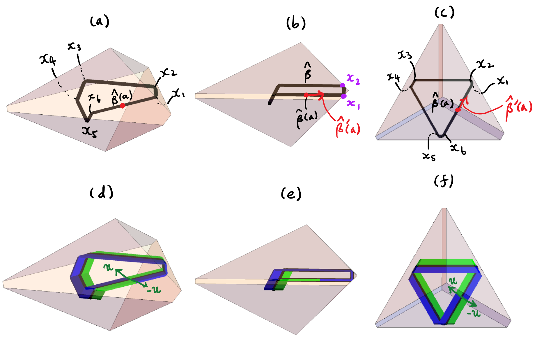
Figure 3.3: (a), (b), (c): Three different views of a folded billiard trajectory $\hat{\beta}$ in the beveling $\operatorname{Bev}(\mathbf{X},\mathcal{F},h)$ from Figure 3.1. (d), (e), (f): Three views of $q(M)\subset\operatorname{Bev}(\mathbf{X},\mathcal{F},h)$, where $q:\mathcal{D}_{\mathrm{}}\operatorname{Bev}(\mathbf{X},\mathcal{F},h)\to\operatorname{Bev}(\mathbf{X},\mathcal{F},h)$ is the quotient map, and $M$ is a flat Möbius strip isometrically embedded in $\mathcal{D}_{\mathrm{}}\operatorname{Bev}(\mathbf{X},\mathcal{F},h)$ such that its core curve is the closed geodesic corresponding to $\hat{\beta}$.

In fact, some tubular neighbourhood of $\hat{\gamma}$ is a maximally twisted tube: at any point $x$ on $\hat{\gamma}$, the parallel transport map $T_{x}\mathcal{D}_{\mathrm{}}\hat{\mathbf{X}}\to T_{x}\mathcal{D}_{\mathrm{}}\hat{\mathbf{X}}$ must be $(-\operatorname{id})$ (negation of the identity) when restricted to the orthogonal complement of $\hat{\gamma}^{\prime}(x)$. This can be derived from the existence of a flat Möbius band $M$ isometrically embedded in $\mathcal{D}_{\mathrm{}}\hat{\mathbf{X}}$ so that its core curve is $\hat{\gamma}$. The image of $M$ under the canonical quotient map $q:\mathcal{D}_{\mathrm{}}\hat{\mathbf{X}}\to\hat{\mathbf{X}}$ is illustrated in Figure 3.3(d)–(f). Observe that $\hat{\beta}$ is the core curve of $q(M)$, and that $q(M)$ appears to be “folded” around the edges of $\mathbf{X}$, which is the reason for saying that crease-like segments “simulate folding”. (Let $v\in T_{x}M$ be orthogonal to $\gamma^{\prime}(x)$, such that $dq_{x}(v)$ is the vector labeled $u$ in Figure 3.3(d). Then parallel transporting $v$ along $\gamma$ moves it along the blue portion of $M$, bringing it back to $-v$. Parallel transporting a vector orthogonal to $M$ at $x$ must also negate it, because parallel transportation preserves the orientation in the orientable $\mathcal{D}_{\mathrm{sm}}\hat{\mathbf{X}}$.) Observe the similarities between Figure 3.3 and Figure 1.1; a similar procedure was used to generate the example illustrated in Figure 1.1.

Eventually we will iterate this beveling construction, producing a sequence $\mathbf{X}^{2},\mathbf{X}^{3},\mathbf{X}^{4},\dotsc$ of convex polytopes with dimensions $2,3,4$ and so on, such that $\operatorname{pr}(\mathbf{X}^{n+1})\subset\mathbf{X}^{n}$. For example, Figure 3.1(a) shows a possible choice for $\mathbf{X}^{2}$, and Figure 3.1(d) shows one view of a possible choice for $\mathbf{X}^{3}$; in this figure it can be seen that $\operatorname{pr}\mathbf{X}^{3}$ is very similar to $\mathbf{X}^{2}$, but the former is a strict subset of the latter. This relation is a consequence of the following lemma:

Lemma 3.4 (Horizontal cross-sections of bevelings).

Let $\mathbf{X}$ be an $n$-polytope, $\mathcal{F}$ be a subset of its faces, and $h:\mathcal{F}\to\mathbb{R}$ be a function. Then $\operatorname{Bev}(\mathbf{X},\mathcal{F},h)\cap\Pi_{r}$ is $\mathbf{X}^{\prime}\times\{r\}$, where $\mathbf{X}^{\prime}$ is the $n$-polytope obtained from $\mathbf{X}$ by, for each $F\in\mathcal{F}$, translating the supporting half-space of $F$ inwards by a distance $\left\lvert r-h(F)\right\rvert$. Consequently, $\operatorname{pr}(\operatorname{Bev}(\mathbf{X},\mathcal{F},h))\subset\mathbf{X}$.

Proof.

For each face $F$ of $\mathbf{X}$, if $F\notin\mathcal{F}$ then $\operatorname{pr}(\mathbf{W}^{h}(F)\cap\Pi_{r})$ is simply the supporting halfspace of $F$. If $F\in\mathcal{F}$ then $\operatorname{pr}(\mathbf{W}^{h}(F)\cap\Pi_{r})$ is the supporting halfspace of $F$ but translated a distance $\left\lvert r-h(F)\right\rvert$ along the inward-pointing unit vector. Therefore the result follows. ∎

The parallel transport maps of folded billiard trajectories in $\mathbf{X}^{n}$ will be related to those of billiard trajectories in $\mathbf{X}^{n+1}$ because the parallel transport maps will be “compatible” with the projections $\operatorname{pr}$, in turn because the reflections about faces of $\mathbf{X}^{n}$ are related to the reflections about faces of $\mathbf{X}^{n+1}$ via $\operatorname{pr}$. This property, which is essential to let us compute parallel transport maps using reflections, will be proven in the next lemma. Let us define some useful notation for reflections associated with a beveling $\operatorname{Bev}(\mathbf{X},\mathcal{F},h)$ of an $n$-polytope $\mathbf{X}$. For each face $F$ of $\mathbf{X}$, let $R_{F}:\mathbb{R}^{n}\to\mathbb{R}^{n}$ be the reflection about $F$, and let $\rho_{F}:\mathbb{R}^{n+1}\to\mathbb{R}^{n+1}$ denote the product of the reflections about the supporting hyperplanes of $\mathbf{W}^{h}(F)$. (There are either one or two supporting hyperplanes, and in the latter case the order of multiplication does not matter.)

Figure 3.4 illustrates some of this notation in the context of a rectangle $\mathbf{X}\subset\mathbb{R}^{2}$ and a beveling $\hat{\mathbf{X}}=\operatorname{Bev}(\mathbf{X},\{F_{1},F_{3}\},h)$, where $h(F_{1})=+\epsilon$ and $h(F_{3})=-\epsilon$ for some $\epsilon>0$. The figure also hints at the compatibility between the projection ($\operatorname{pr}:\mathbb{R}^{3}\to\mathbb{R}^{2}$ in this case) and the reflections: from the figure it can be seen that $\operatorname{pr}(\rho_{F_{1}}(\hat{\mathbf{X}}))=R_{F_{1}}(\mathbf{X})=R_{F_{1}}(\operatorname{pr}(\hat{\mathbf{X}}))$. This phenonenon can be rigorously generalized into our next lemma.

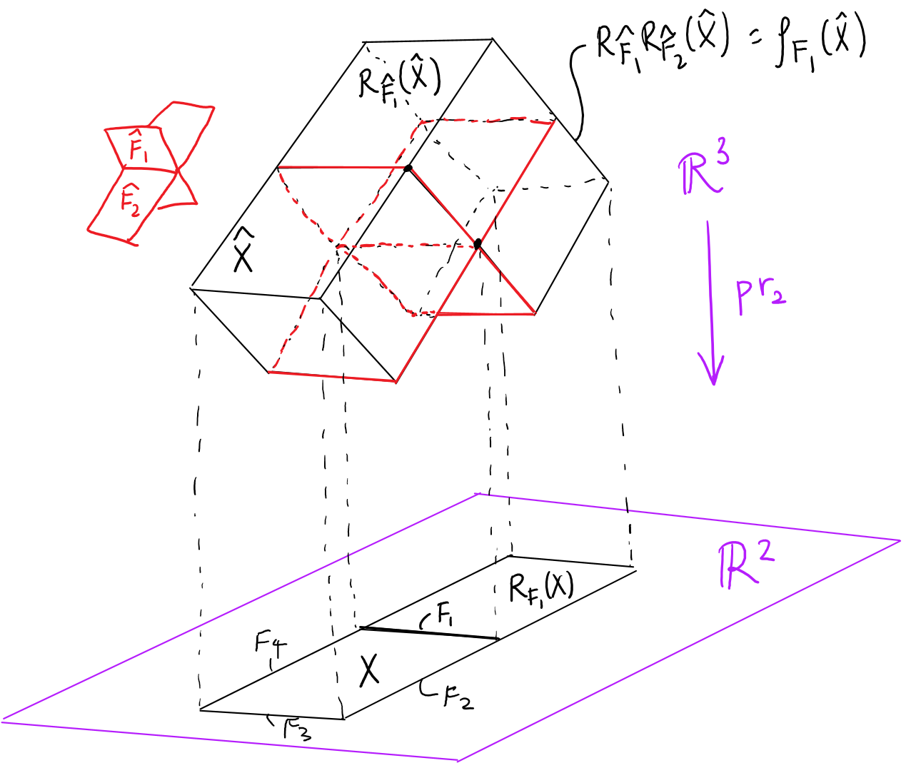
Figure 3.4: The relationships between a polygon $\mathbf{X}$, its beveling $\hat{\mathbf{X}}$, the projection $\operatorname{pr}$ and the transformations $R_{F_{i}}$, $R_{\hat{F}_{j}}$, and $\rho_{F_{i}}$. Here $\mathbf{X}$ is a rectangle with faces $F_{1},\dotsc,F_{4}$, and $\hat{\mathbf{X}}=\operatorname{Bev}(\mathbf{X},\{F_{1},F_{3}\},h)$, where $h(F_{1})=+\epsilon$ and $h(F_{3})=-\epsilon$ for some $\epsilon>0$. Two of the faces of $\hat{\mathbf{X}}$ are denoted $\hat{F}_{1}$ and $\hat{F}_{2}$.

Before we state our next lemma we need some additional notation. If $V$ is a subspace of $\mathbb{R}^{n}$, let $V^{\perp}$ denote its orthogonal complement. Suppose that $V,W$ are subspaces of $\mathbb{R}^{n}$ such that $V+W=\mathbb{R}^{n}$ and $V\cap W=\{0\}$. Then we write $\mathbb{R}^{n}=V\oplus W$. We will write $\mathbb{R}^{m+n}=\mathbb{R}^{m}\oplus\mathbb{R}^{n}$ to mean $\mathbb{R}^{m+n}=\mathbb{R}^{m}\times\{0\}\oplus\{0\}\times\mathbb{R}^{n}$, where $\mathbb{R}^{m}\times\{0\}$ and $\{0\}\times\mathbb{R}^{n}$ are subspaces of $\mathbb{R}^{m+n}$. Furthermore, if $C:\mathbb{R}^{n}\to\mathbb{R}^{n}$ is a linear operator that restricts to $A:V\to V$ and $B:W\to W$, then we write $C=A\oplus B$. Let $\operatorname{id}_{V}$ denote the identity map on $V$.

Lemma 3.5 (Compatibility with projection).

Let $\operatorname{Bev}(\mathbf{X},\mathcal{F},h)$ be a beveling of an $n$-polytope $\mathbf{X}$. Then for each face $F$ of $\mathbf{X}$,

$${\operatorname{pr}}\circ\rho_{F}=R_{F}\circ\operatorname{pr}.$$ (3.2)

Moreover, $\Pi_{0}=\mathbb{R}^{n}\times\{0\}$ is an invariant subspace of $d\rho_{F}$ and with respect to the decomposition $\mathbb{R}^{n+1}=\Pi_{0}\oplus\Pi_{0}^{\perp}\simeq\mathbb{R}^{n}\oplus\mathbb{R}$,

$$d\rho_{F}=dR_{F}\oplus(-\det d\rho_{F})\text{, where }\det d\rho_{F}=\begin{cases}+1&F\in\mathcal{F}\\ -1&F\notin\mathcal{F}.\end{cases}$$ (3.3)

Proof.

We will prove Equation 3.3 and then derive Equation 3.2 from it. Let $v$ be a normal vector of $F$ in $\mathbf{X}$ and let its span be $V$ (see Figure 3.5(a)). Then under the decomposition $\mathbb{R}^{n}=V^{\perp}\oplus V\simeq\mathbb{R}^{n-1}\oplus\mathbb{R}$, we may write $dR_{F}$ as $\operatorname{id}_{V^{\perp}}\oplus(-1)$ because by definition of a reflection, $dR_{F}(v)=-v$ and $dR_{F}$ must fix every vector in the hyperplane of reflection. Let $u=(0,\dotsc,0,1)\in\mathbb{R}^{n+1}$, and let $W=\operatorname{span}\{(v,0),u\}$.

Now we work with the decomposition $\mathbb{R}^{n+1}=W^{\perp}\oplus W\simeq\mathbb{R}^{n-1}\oplus\mathbb{R}^{2}$, and use $(v,0),u$ as a basis of $W$.

• If $F\notin\mathcal{F}$, let $\hat{F}$ be the face of $\operatorname{Bev}(\mathbf{X},\mathcal{F},h)$ that is inherited from $\mathbf{W}^{h}(F)$. Then $d\rho_{F}=dR_{\hat{F}}=\operatorname{id}_{W^{\perp}}\oplus\left[\begin{smallmatrix}-1&0\\ 0&1\end{smallmatrix}\right]$ because $d\rho_{F}$ is a reflection that should send $(v,0)$ to $(-v,0)$. Moreover, $d\rho_{F}$ should fix $u$ and any vector in $W^{\perp}$ because they all lie in the hyperplane of reflection. Equation 3.3 follows as a result.

• On the other hand, if $F\in\mathcal{F}$, then let $\hat{F}$ and $\hat{F}^{\prime}$ be the two faces of $\operatorname{Bev}(\mathbf{X},\mathcal{F},h)$ that are inherited from $\mathbf{W}^{h}(F)$; order them so that $dR_{\hat{F}}$ sends $(v,0)\mapsto u$ and vice versa, while $dR_{\hat{F}^{\prime}}$ sends $(v,0)\mapsto-u$ and $u\mapsto-(v,0)$ (see Figure 3.5(b)). Meanwhile, $W^{\perp}$ lies in the hyperplane of reflection of both $dR_{\hat{F}}$ and $dR_{\hat{F}^{\prime}}$. Hence, using the decomposition $\mathbb{R}^{n+1}=W^{\perp}\oplus W$ and the basis $(u,0),v$ of $W$, we can write $dR_{\hat{F}}=\operatorname{id}_{W^{\perp}}\oplus\left[\begin{smallmatrix}0&1\\ 1&0\end{smallmatrix}\right]$ and $dR_{\hat{F}^{\prime}}=\operatorname{id}_{W^{\perp}}\oplus\left[\begin{smallmatrix}0&-1\\ -1&0\end{smallmatrix}\right]$. Therefore $d\rho_{F}=dR_{\hat{F}}dR_{\hat{F}^{\prime}}=\operatorname{id}_{W^{\perp}}\oplus\left[\begin{smallmatrix}-1&0\\ 0&-1\end{smallmatrix}\right]$.

From this representation, noting that $\Pi_{0}=W^{\perp}\oplus\operatorname{span}\{(v,0)\}$, we can see that $\Pi_{0}$ is always an invariant subspace of $d\rho_{F}$. Equation 3.3 then follows, which implies that ${\operatorname{pr}}\circ d\rho_{F}=dR_{F}\circ\operatorname{pr}$. Note that since $R_{F}$ is an affine transformation, $R_{F}=T_{x}\circ dR_{F}\circ T_{-x}$, where $T_{x}$ denotes translation by a vector $x\in F$. Similarly, $\rho_{F}=T_{(x,h(F))}\circ d\rho_{F}\circ T_{(-x,-h(F))}$. Therefore

$${\operatorname{pr}}\circ\rho_{F} ={\operatorname{pr}}\circ T_{(x,h(F))}\circ d\rho_{F}\circ T_{(-x,-h(F))}$$ (3.4)

$$=T_{x}\circ{\operatorname{pr}}\circ d\rho_{F}\circ T_{(-x,-h(F))}$$ (3.5)

$$=T_{x}\circ dR_{F}\circ{\operatorname{pr}}\circ T_{(-x,-h(F))}$$ (3.6)

$$=T_{x}\circ dR_{F}\circ T_{-x}\circ{\operatorname{pr}}$$ (3.7)

$$=R_{F}\circ{\operatorname{pr}}.$$ (3.8)

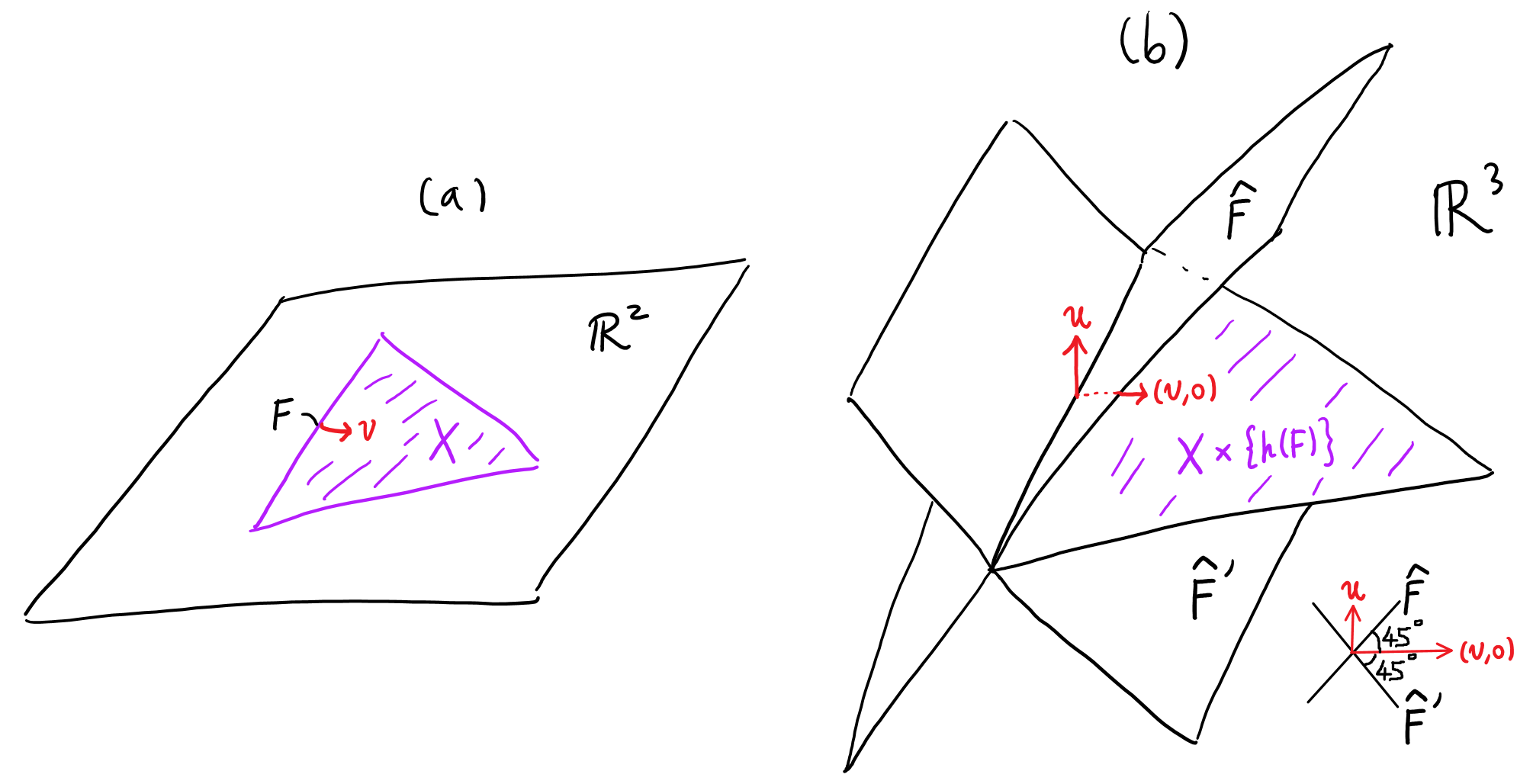
Figure 3.5: (a) An illustration of some notation from the proof of Lemma 3.5, when $\mathbf{X}$ is an equilateral triangle. (b) An illustration of the notation for the case in the proof where $F\in\mathcal{F}$.

∎

As a consequence of the previous results, we can derive the following relationship between the parallel transport maps of billiard trajectories $\beta$ and $\hat{\beta}$, where $\hat{\beta}$ is a folded billiard trajectory in a beveling that simulates colliding at the same faces that $\beta$ collides at.

Lemma 3.6.

Let $\beta$ be a billiard trajectory in $\mathbf{X}$ that collides at faces $F_{1},\dotsc,F_{k}$. Let $\hat{\mathbf{X}}=\operatorname{Bev}(\mathbf{X},\mathcal{F},h)$ be a beveling of $\mathbf{X}$, and suppose that $\hat{\beta}$ is a folded billiard trajectory in $\hat{\mathbf{X}}$ that simulates colliding at $F_{1},\dotsc,F_{k}$. Assume further that $\hat{\beta}$ collides with every face inherited from $\mathbf{W}^{h}(F_{k})$. Then the parallel transport maps $P:\mathbb{R}^{n}\to\mathbb{R}^{n}$ and $\hat{P}:\mathbb{R}^{n+1}\to\mathbb{R}^{n+1}$ of $\beta$ and $\hat{\beta}$ respectively (where tangent spaces have been canonically identified with ambient Euclidean spaces) are related by

$$\hat{P}=P\oplus(-1)^{\left\lvert\mathcal{F}^{\prime}\right\rvert},$$ (3.9)

with respect to the decomposition $\mathbb{R}^{n+1}\simeq\mathbb{R}^{n}\oplus\mathbb{R}$, and where $\mathcal{F}^{\prime}$ is the subset of faces in $\mathcal{F}$ that $\beta$ collides with. The number of collisions of $\hat{\beta}$ is also $\left\lvert\mathcal{F}^{\prime}\right\rvert$ more than that of $\beta$.

Proof.

We may assume that both billiard trajectories collide at most once with each face, as the general case follows in the same manner. For the number of collisions, observe from Figure 3.2 that $\hat{\beta}$ experiences two collisions with faces inherited from $\mathbf{W}^{h}(F_{i})$ if $F_{i}\in\mathcal{F}$, otherwise it collides only once with a face inherited from $\mathbf{W}^{h}(F_{i})$. Either way, $\beta$ only collides once with $F_{i}$.

Note that $P=dR_{F_{k}}\dotsm dR_{F_{1}}$ and $\hat{P}=d\rho_{F_{k}}\dotsm d\rho_{F_{1}}$, and the rest follows from Equation 3.3. ∎

3.2 Properties of folded billiard trajectories

The hypotheses of Lemma 3.6 require that $\hat{\beta}$ simulates colliding at the same faces that $\beta$ collides at. We will prove Proposition 3.8 which asserts that under certain conditions, this occurs when $\beta$ is derived in a particular manner from ${\operatorname{pr}}\circ\hat{\beta}$.

To prove that, we will need to study the segments of $\hat{\beta}$. The example in Figure 3.3(a)–(c) of a billiard trajectory in a beveling $\operatorname{Bev}(\mathbf{X},\mathcal{F},h)$ has crease-like segments are $x_{1}x_{2}$, $x_{3}x_{4}$ and $x_{5}x_{6}$. Its other segments are horizontal. Hence the billiard trajectory begins with a horizontal segment, collides with a face of $\mathbf{W}^{h}(F)$ for some $F\in\mathcal{F}$, continues along a creaselike segment, collides with the other face of $\mathbf{W}^{h}(F)$, proceeds along a horizontal segment, and the same repeats. If, for some other beveling, a horizontal segment of the billiard trajectory collides with the face of $\mathbf{W}^{h}(F)$ for some $F\notin\mathcal{F}$, then the trajectory would continue along another horizontal segment. (Compare with Figure 3.2.) The behaviour outlined above is confirmed by Lemma 3.7 and Proposition 3.8.

Lemma 3.7.

Let $\operatorname{Bev}(\mathbf{X},\mathcal{F},h)$ be a beveling of an $n$-polytope $\mathbf{X}$ with a folded billiard trajectory $\hat{\beta}:[a,b]\to\operatorname{Bev}(\mathbf{X},\mathcal{F},h)$. Then each segment of $\hat{\beta}$ is horizontal if and only if it is not crease-like. Consequently, the first segment of $\hat{\beta}$ cannot be crease-like. Moreover, the segments before and after a crease-like segment must be horizontal.

Proof.

The definition of a folded billiard trajectory requires the first segment of $\hat{\beta}$ to be horizontal. Let $\hat{\beta}$ simulate colliding at $F_{1},\dotsc,F_{k}$. Suppose that $F_{1}\notin\mathcal{F}$. Then the velocity vector of $\hat{\beta}$ just after the first collision is obtained by reflecting $\hat{\beta}^{\prime}(a)$ about the hyperplane through the origin that is parallel to $\partial\mathbf{W}^{h}(F_{1})$. Therefore the second segment of $\hat{\beta}$ would also be horizontal. Repeating the same argument shows that if $F_{1},\dotsc,F_{j}\notin\mathcal{F}$ then the first $j+1$ segments of $\hat{\beta}$ will be horizontal. Now suppose that $F_{j+1}\in\mathcal{F}$. Let $\hat{F},\hat{F}^{\prime}$ be the faces of $\operatorname{Bev}(\mathbf{X},\mathcal{F},h)$ inherited from $\mathbf{W}^{h}(F_{j+1})$, among which $\hat{\beta}$ collides with $\hat{F}$ first at time $t$ (and may or may not collide with $\hat{F}^{\prime}$). Just before time $t$, $\hat{\beta}$ is traveling on a horizontal segment $\eta$, and some elementary geometry will verify that the segment $\sigma$ after time $t$ satisfies the definition of a crease-like segment. If $\sigma$ is not the final segment, then the definition of a folded billiard trajectory requires that $\hat{\beta}$ collides with $\hat{F}^{\prime}$ next. Therefore the velocity vector of the next segment is obtained from that of $\eta$ via the transformation $dR_{\hat{F}^{\prime}}dR_{\hat{F}}=d\rho_{F_{j+1}}$, so by Lemma 3.5 the next segment is horizontal again. By continuing to apply the above arguments, we can show that all of the segments of $\hat{\beta}$ are either horizontal or crease-like. ∎

Proposition 3.8.

Let $\operatorname{Bev}(\mathbf{X},\mathcal{F},h)$ be a beveling of an $n$-polytope $\mathbf{X}$, and $\hat{\beta}:[a,b]\to\operatorname{Bev}(\mathbf{X},\mathcal{F},h)$ be a folded billiard trajectory that simulates colliding at $F_{1},\dotsc,F_{i^{*}}$. (If $\hat{\beta}$ has no collisions, i.e. it is a line segment, then $i^{*}=0$.). Then

1. For each crease-like segment $\sigma$ of $\hat{\beta}$ that simulates folding around $F$, ${\operatorname{pr}}\circ\sigma$ is at constant distance $d_{\sigma}=\left\lvert\operatorname{height}(x)-h(F)\right\rvert>0$ away from the supporting hyperplane of $F$, where $x$ is the point from which $\sigma$ begins.

If the final segment of $\hat{\beta}$ is horizontal then the following statements also hold:

1. Suppose that among the faces that $\hat{\beta}$ simulates colliding at, $F_{m_{1}},\dotsc,F_{m_{k}}$ are those that lie in $\mathcal{F}$, where $1\leq m_{1}<\dotsb<m_{k}\leq i^{*}$. Then

   $$\operatorname{height}(\hat{\beta}(b))=2\big{(}h(F_{m_{k}})-h(F_{m_{k-1}})+\dotsb+(-1)^{k-1}h(F_{m_{1}})\big{)}+(-1)^{k}\operatorname{height}(\hat{\beta}(a)).$$ (3.10)

2. There are $i^{*}+1$ horizontal segments $\eta_{0},\eta_{1},\dotsc,\eta_{i^{*}}$, listed in the order they are traversed by $\hat{\beta}$. For each $1\leq i\leq i^{*}$, the lines containing ${\operatorname{pr}}\circ\eta_{i-1}$ and ${\operatorname{pr}}\circ\eta_{i}$ intersect the supporting hyperplane of $F_{i}$ at the same point $x_{i}$. Assume further that each $x_{i}$ lies in the interior of $F_{i}$. Then $\operatorname{pr}(\hat{\beta}(a)),x_{1},\dotsc,x_{i^{*}},\operatorname{pr}(\hat{\beta}(b))$ is a billiard trajectory $\beta:[a,b]\to\mathbf{X}$ of the same length as $\hat{\beta}$. (If $\hat{\beta}$ has no collisions, then $\operatorname{pr}(\hat{\beta}(a)),\operatorname{pr}(\hat{\beta}(b))$ is a billiard trajectory in $\mathbf{X}$ that is also a line segment.)

3. Assuming that all of (iii) holds,

   $$\operatorname{dist}(\operatorname{pr}(\hat{\beta}(t)),\beta(t))\leq\max_{\sigma}d_{\sigma}\qquad\text{for all }t\in[a,b],$$ (3.11)

   where the maximum is taken over all crease-like segments $\sigma$ of $\hat{\beta}$. Furthermore, $\operatorname{pr}(\hat{\beta}(t))=\beta(t)$ whenever $\hat{\beta}(t)$ lies on a horizontal segment.

Remark 3.9.

Before we proceed to the proof, we note that Equation 3.10 is satisfied by the $\hat{\beta}$ illustrated in Figure 3.3: note that in this example, $\mathbb{R}^{2}\times\{h(F_{1})\}$ lies exactly halfway in height between the horizontal segments $\eta_{0}=\hat{\beta}(a)x_{1}$ and $\eta_{1}=x_{2}x_{3}$ (compare Figure 3.3(b) with Figure 3.1(f)). Hence, $h(F_{1})=\frac{1}{2}(\operatorname{height}(\eta_{0})+\operatorname{height}(\eta_{1}))$. Statement (i) can also be partially verified in the same example: when the crease-like segment $x_{1}x_{2}$ is depicted in Figure 3.3(c) using the projection $\operatorname{pr}$, it looks parallel to $F_{1}$ in Figure 3.1(a). (Compare also with Figure 3.6.) Statement (iii) is also satisfied by the same example: The billiard trajectory in $\mathbf{X}$ obtained by applying Statement (iii) to the $\hat{\beta}$ in Figure 3.3 is precisely $\beta$ from Figure 3.1(a). Statement (iv) essentially asserts that ${\operatorname{pr}}\circ\hat{\beta}$ stays “close” to $\beta$; this property can be observed by comparing Figure 3.1(a) to Figure 3.3(c).

When the assumptions of Statement (iii) are satisfied, the resulting billiard trajectory in $\mathbf{X}$ (or a slight modification) will play the role of $\beta_{n}$ from the discussion at the beginning of Section 3, while $\hat{\beta}$ will play the role of $\beta_{n+1}$.

Figure 3.6: The crease-like segments $\sigma_{1}$, $\sigma_{2}$ and $\sigma_{3}$ of a folded billiard trajectory $\hat{\beta}$ in the beveling $\operatorname{Bev}(\mathbf{X},\mathcal{F},h)$ from Figure 3.3. Viewed from this orientation, the projections of each $\sigma_{i}$ can be seen to satisfy Proposition 3.8(i).

Proof.

The elements of our proof will be illustrated in Figures 3.7 and 3.8, in the context of the $\mathbf{X}$ and $\hat{\mathbf{X}}=\operatorname{Bev}(\mathbf{X},\mathcal{F},h)$ from Figure 3.4. To simplify notation, we will write $\hat{\mathbf{X}}_{1}=\rho_{F_{1}}(\hat{\mathbf{X}})$. Note that in this situation, the face $F_{1}$ lies in $\mathcal{F}=\{F_{1},F_{3}\}$.

(i): Suppose that $\sigma$ is a crease-like segment that simulates folding around the face $F_{i}$. This segment must start from some point $x$ in a face $\hat{F}$ of $\operatorname{Bev}(\mathbf{X},\mathcal{F},h)$ that is inherited from $\mathbf{W}^{h}(F_{i})$. $\sigma$ must be preceded by a horizontal segment $\eta$ by Lemma 3.7, and the definition of a billiard trajectory implies that $R_{\hat{F}}\circ\sigma$ and $\eta$ lie on the same horizontal line. (This is illustrated in Figure 3.7(a) in the case where $i=1$; in this scenario, $\eta=\eta_{0}$ and $R_{\hat{F}}\circ\sigma=\hat{\ell}_{1}$.) Let $\Pi$ be the supporting hyperplane of $F_{i}$. Then for every point $y\in\sigma$, $\operatorname{dist}(\operatorname{pr}(y),\Pi)=\operatorname{dist}(y,\Pi\times\mathbb{R})=\operatorname{dist}(R_{\hat{F}}(y),R_{\hat{F}}(\Pi\times\mathbb{R}))$. It can be seen that $R_{\hat{F}}(\Pi\times\mathbb{R})=\mathbb{R}^{2}\times\{h(F_{i})\}$. Therefore $\operatorname{dist}(R_{\hat{F}}(y),\mathbb{R}^{2}\times\{h(F_{i})\})=\operatorname{dist}(\eta,\mathbb{R}^{2}\times\{h(F_{i})\})=\left\lvert\operatorname{height}(x)-h(F_{i})\right\rvert$. This number should be positive, because $x$ should lie in the interior of $\mathbf{W}^{h}(F_{i})$.

Henceforth we will assume that the final segment of $\hat{\beta}$ is horizontal. The proof of Lemma 3.7—in particular, how $\hat{\beta}$ switches from horizontal segments to crease-like segments and vice versa—implies that there are $i^{*}+1$ horizontal segments, $\eta_{0},\eta_{1},\dotsc,\eta_{i^{*}}$.

(ii): We use the standard technique of “unraveling” a billiard trajectory into a straight line. Let $\hat{\ell}:[a,b]\to\mathbb{R}^{n+1}$ be a line segment that extends the first segment of $\hat{\beta}$ forward at a constant velocity equal to $\hat{\beta}^{\prime}(a)$ (see Figure 3.7(a)). Since the first segment of $\hat{\beta}$ is horizontal by the definition of a folded billiard trajectory, $\hat{\ell}$ must also be horizontal. Suppose that $\hat{\beta}$ collides with $j^{*}$ faces $\hat{F}_{1},\dotsc,\hat{F}_{j^{*}}$ of $\hat{\mathbf{X}}=\operatorname{Bev}(\mathbf{X},\mathcal{F},h)$. Then $\hat{\beta}$ is the concatenation of several segments $R_{\hat{F}_{j}}\dotsm R_{\hat{F}_{1}}\circ\hat{\ell}_{j}$, where $\hat{\ell}_{j}$ is the restriction of $\hat{\ell}$ to the portion that lies in $R_{\hat{F}_{1}}\dotsm R_{\hat{F}_{j}}(\hat{\mathbf{X}})$ (see Figure 3.7(a)). This implies that for each $1\leq i\leq i^{*}$, $\eta_{i}$ is a restriction of $\rho_{F_{i}}\dotsm\rho_{F_{1}}\circ\hat{\ell}$, where the $R$’s have been grouped into $\rho$’s. (This is possible because $\eta_{i}$ cannot be a crease-like segment by Lemma 3.7.) Therefore $\rho_{F_{i}}\circ\eta_{i-1}$ and $\eta_{i}$ lie on the same line, and have the same height.

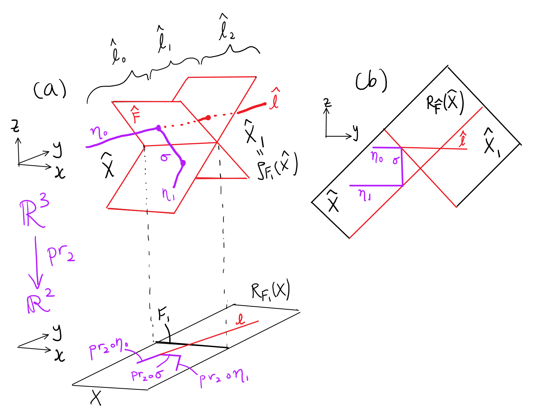
Figure 3.7: An illustration of the objects and notations from Proposition 3.8, in the context of the $\mathbf{X}$ and $\hat{\mathbf{X}}=\operatorname{Bev}(\mathbf{X},\mathcal{F},h)$ from Figure 3.4, where $\hat{\mathbf{X}}_{1}$ refers to $\rho_{F_{1}}(\hat{\mathbf{X}})$. Note that the intersecting red polygons in (a) are the same as those in Proposition 3.8. (b) is a view of part of (a) from a different direction.

From the proof of Lemma 3.5, $d\rho_{F}$ can be expressed in terms of a matrix that depends on whether $F\in\mathcal{F}$ or $F\notin\mathcal{F}$. Whenever $d\rho_{F}(u)=v$, if $F\notin\mathcal{F}$ then $\operatorname{height}(u)=\operatorname{height}(v)$, whereas if $F\in\mathcal{F}$ then $\operatorname{height}(u)=-\operatorname{height}(v)$. Now suppose that $\rho_{F}(x)=y$. From the expression of $\rho_{F}$ as the conjugate of $d\rho_{F}$ by a translation (again from the proof of Lemma 3.5), if $F\notin\mathcal{F}$ then $x$ and $y$ have the same height. On the other hand, if $F\in\mathcal{F}$, then $\operatorname{height}(y)$ is the reflection, in $\mathbb{R}$, of $\operatorname{height}(x)$ about $h(F)$. Thus the following recurrence relation can be deduced from the fact that $\rho_{F_{i}}\circ\eta_{i-1}$ and $\eta_{i}$ lie on the same line: For each $1\leq i\leq i^{*}$, the heights of $\eta_{i-1}$ and $\eta_{i}$ satisfy the recurrence relation

$$\operatorname{height}(\eta_{i})=\begin{cases}\operatorname{height}(\eta_{i-1})&F_{i}\notin\mathcal{F}\\ 2h(F_{i})-\operatorname{height}(\eta_{i-1})&F_{i}\in\mathcal{F}.\end{cases}$$ (3.12)

Equation 3.10 can be derived from this recurrence relation.

(iii): As with our proof of (ii), $\hat{\beta}$ can be analysed by “unraveling” it into a line segment $\hat{\ell}$ passing through copies of $\operatorname{Bev}(\mathbf{X},\mathcal{F},h)$ that are transformed by a series of reflections. The $\hat{\mathbf{X}}_{1}$ we defined at the beginning of the proof is one of them while some others are of the form $\hat{\mathbf{X}}_{i}=\rho_{F_{1}}\dotsm\rho_{F_{i}}(\operatorname{Bev}(\mathbf{X},\mathcal{F},h))$. Under this “unravelling”, each $\eta_{i}$ corresponds to a transformed copy $\eta_{i}^{*}=\rho_{F_{1}}\dotsm\rho_{F_{i}}\circ\eta_{i}$ that is the restriction of $\hat{\ell}$ to the portion that lies inside $\hat{\mathbf{X}}_{i}$. (In Figure 3.7(a), $\eta_{0}^{*}$ is $\hat{\ell}_{0}$ and $\eta_{1}^{*}$ is $\hat{\ell}_{2}$. $\eta_{0}^{*}$ and $\eta_{1}^{*}$ are also depicted in Figure 3.8(a).) Consider a similar setup for $\mathbf{X}$: $\ell={\operatorname{pr}}\circ\hat{\ell}:[a,b]\to\mathbb{R}^{n}$ is the line segment that starts from $\operatorname{pr}(\hat{\beta}(a))$ (which lies in $\mathbf{X}$ due to Lemma 3.4) with constant velocity equal to $\operatorname{pr}(\hat{\beta}^{\prime}(a))$ (see Figure 3.7(a) and Figure 3.8(b)). $\ell$ passes through transformed copies of $\mathbf{X}$ of the form $\mathbf{X}_{i}=R_{F_{1}}\dotsm R_{F_{i}}(\mathbf{X})$. Each line segment ${\operatorname{pr}}\circ\eta_{i}^{*}$ is a restriction of $\ell$ into a line segment that lies in $\mathbf{X}_{i}$ (because of Lemma 3.4) but that may not touch $\partial\mathbf{X}_{i}$ (see Figure 3.8(b)). To prove (iii), we essentially want to show that if we extend these segments all the way to touch $\partial\mathbf{X}_{i}$ and then transform the extended segments back into $\mathbf{X}$ via sequences of reflections $R_{F_{i}}\dotsm R_{F_{1}}$, then they will form a billiard trajectory.

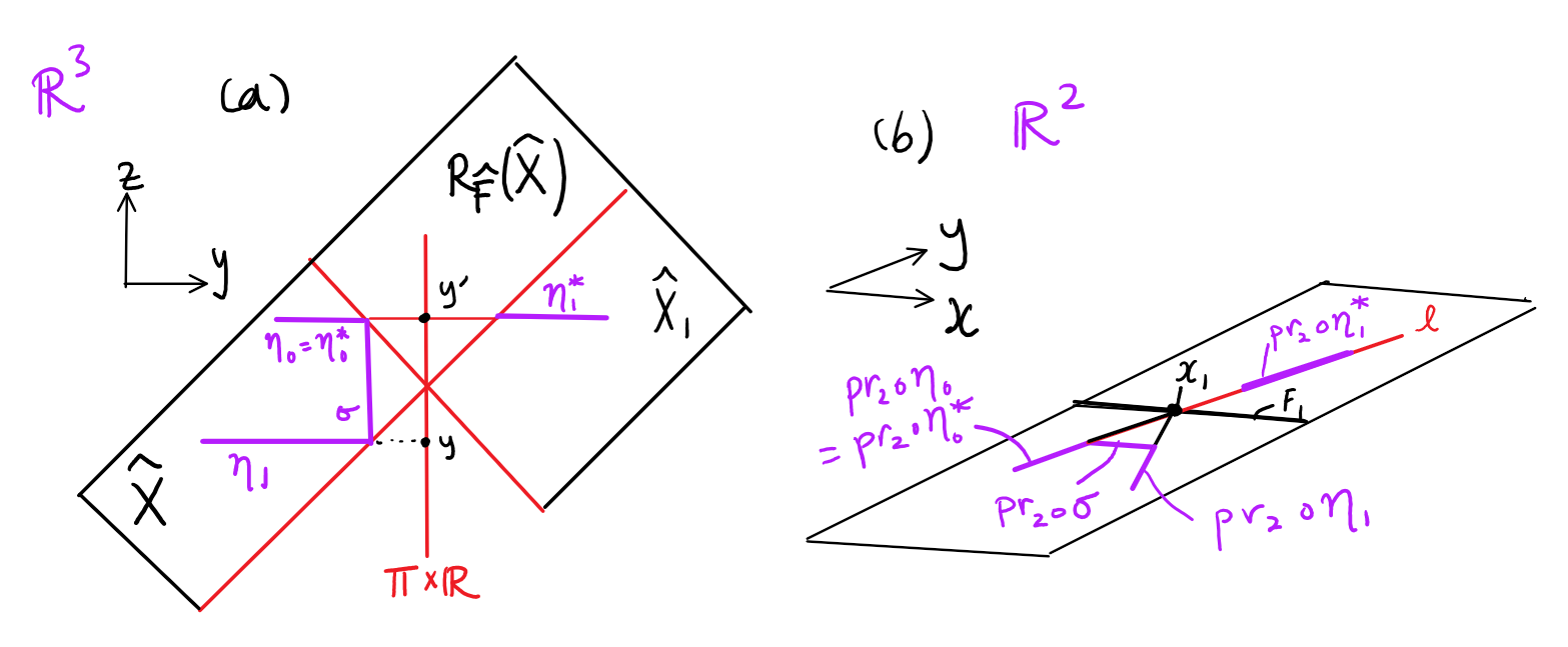
Figure 3.8: An illustration of some notation from the proof of Proposition 3.8(iii), in the same example as Figure 3.4 and assuming that $i=1$. Note that in this case, $x_{1}^{*}=x_{1}$.

Equation 3.2 implies that

$${\operatorname{pr}}\circ\eta_{i}^{*}={\operatorname{pr}}\circ\rho_{F_{1}}\dotsm\rho_{F_{i}}\circ\eta_{i}=R_{F_{1}}\dotsm R_{F_{i}}\circ{\operatorname{pr}}\circ\eta_{i}.$$ (3.13)

This helps us to translate Statement (iii) into a statement in terms of the $\eta_{i}^{*}$’s. Consider any $1\leq i\leq i^{*}$, and let $\Pi$ be the supporting hyperplane of $F_{i}$. First of all, note that the line containing $\eta_{i}$ must intersect $\Pi\times\mathbb{R}$ transversally at some point $y$, because of the horizontal nature of $\eta_{i}$ and the fact that, as part of a billiard trajectory, $\eta_{i}$ cannot be parallel to any face of $\operatorname{Bev}(\mathbf{X},\mathcal{F},h)$. Similarly, the line containing $\eta_{i-1}$ must intersect $\Pi\times\mathbb{R}$ transversally at some point $y^{\prime}$. ($\Pi\times\mathbb{R}$, $y$ and $y^{\prime}$ are depicted in Figure 3.8(a), in the case where $i=1$.) Therefore ${\operatorname{pr}}\circ\eta_{i}$ extends to a line that intersects $\Pi$ at $\operatorname{pr}(y)$, and this is equivalent, by Equation 3.13, to the fact that ${\operatorname{pr}}\circ\eta_{i}^{*}$ extends to a line that intersects $R_{F_{1}}\dotsm R_{F_{i}}(\Pi)$ at $R_{F_{1}}\dotsm R_{F_{i}}(\operatorname{pr}(y))$. Similarly, ${\operatorname{pr}}\circ\eta_{i-1}$ extends to a line that intersects $\Pi$ at $\operatorname{pr}(y^{\prime})$, and that is equivalent to the fact that ${\operatorname{pr}}\circ\eta_{i-1}^{*}$ extends to a line that intersects $R_{F_{1}}\dotsm R_{F_{i-1}}(\Pi)$ at $R_{F_{1}}\dotsm R_{F_{i-1}}(\operatorname{pr}(y^{\prime}))$. On the other hand, observe that ${\operatorname{pr}}\circ\eta_{i-1}^{*}$ and ${\operatorname{pr}}\circ\eta_{i}^{*}$ must extend into the same line segment $\ell$ (see Figure 3.8(b)), and $R_{F_{1}}\dotsm R_{F_{i}}(\Pi)=R_{F_{1}}\dotsm R_{F_{i-1}}(\Pi)$ because $R_{F_{i}}$ must fix $\Pi$. Therefore the two points $R_{F_{1}}\dotsm R_{F_{i}}(\operatorname{pr}(y))$ and $R_{F_{1}}\dotsm R_{F_{i-1}}(\operatorname{pr}(y_{i}^{\prime}))$ must be the same point $x_{i}^{*}$. Since $R_{F_{i}}$ fixes $\operatorname{pr}(y)\in\Pi$, we can conclude that $\operatorname{pr}(y)$ and $\operatorname{pr}(y^{\prime})$ are the same point $x_{i}$ that is required in Statement (iii). (When $i=1$, $x_{1}=x_{1}^{*}$, and this point is depicted in Figure 3.8(b).)

Now we assume that $x_{i}$ lies in the interior of $F_{i}$. Translating this to the “unraveling”, this means that $x_{i}^{*}$ lies in the interior of a face of $\mathbf{X}_{i}$ (which is also a face of $\mathbf{X}_{i-1}$). However this implies that $\ell$ is partitioned into segments by the points $x_{1}^{*},\dotsc,x_{i^{*}}^{*}$, and each of those segments lie in some $\mathbf{X}_{i}$. We may then “reverse the unraveling” by transforming each segment in $\mathbf{X}_{i}$ back into $\mathbf{X}$ via $R_{F_{i}}\dotsm R_{F_{1}}$ to get a billiard trajectory $\operatorname{pr}(\hat{\beta}(a)),x_{1},\dotsc,x_{i^{*}},\operatorname{pr}(\hat{\beta}(b))$. Denote this billiard trajectory by $\beta:[a,b]\to\mathbf{X}$.

The conclusion that $\beta$ has the same length as $\hat{\beta}$ can be derived from the preservation of length by the process of “unraveling” $\hat{\beta}$ into $\hat{\ell}$, projecting it via $\operatorname{pr}$ into $\ell$, and “reversing the unraveling”.

(iv): When $\hat{\beta}(s)$ lies on $\eta_{i}$, it corresponds to the point $\hat{\ell}(s)\in\eta_{i}^{*}\subset\hat{\mathbf{X}}_{i}$ and thus $\ell(s)=\operatorname{pr}(\hat{\ell}(s))\in\mathbf{X}_{i}$. ($\operatorname{pr}(\hat{\mathbf{X}}_{i})\subset\mathbf{X}_{i}$ because of Equation 3.13 and Lemma 3.4.) Therefore we may apply Equation 3.13 again to get $\beta(s)=R_{F_{i}}\dotsm R_{F_{1}}\circ\operatorname{pr}(\hat{\ell}(s))={\operatorname{pr}}\circ\rho_{F_{i}}\dotsm\rho_{F_{1}}(\hat{\ell}(s))=\operatorname{pr}(\hat{\beta}(s))$.

Therefore it suffices to prove Equation 3.11 for all $s\in[a,b]$ such that $\hat{\beta}(s)$ lies in the interior of a crease-like segment $\sigma$ or is the ending point of $\sigma$. Let $\sigma$ simulate folding around $F_{i}$, and let $\sigma$ start from a point on a face $\hat{F}$ of $\hat{\mathbf{X}}$. For simplicity’s sake, let us assume that $i=1$; the argument will not change much. Let $\mathbf{W}=\mathbf{W}^{h}(F_{1})$. Then in the unraveling, $\sigma$ corresponds to a segment of $\hat{\ell}$, namely $\hat{\ell}|_{[u,v]}$, that lies in $R_{\hat{F}}(\hat{\mathbf{X}})\subset R_{\hat{F}}(\mathbf{W})$ (see Figure 3.9(a)). In the unraveling, $\beta|_{[u,v]}$ corresponds to $\ell|_{[u,v]}$, which we will compare to $\hat{\ell}|_{[u,v]}$ indirectly by using another line segment $\mu:[u,v]\to\mathbb{R}^{n+1}$ that is obtained by translating $\hat{\ell}|_{[u,v]}$ “vertically”—that is, by changing the last coordinate of every point until the line segment passes through $F_{i}\times\{h(F_{i})\}$ (see Figure 3.9(a)). $\mu$ serves as a good proxy for $\ell|_{[u,v]}$ because ${\operatorname{pr}}\circ\mu={\operatorname{pr}}\circ\hat{\ell}|_{[u,v]}=\ell|_{[u,v]}$, $\mu$ lies entirely in $\mathbf{W}\cup\rho_{F_{1}}(\mathbf{W})$, $\operatorname{pr}(\mu\cap\mathbf{W})$ is the portion of $\beta|_{[u,v]}$ before a collision, and $\operatorname{pr}(\rho_{F_{1}}(\mu\cap\rho_{F_{1}}(\mathbf{W})))$ is the portion of $\beta|_{[u,v]}$ after a collision (see Figure 3.9(b)).

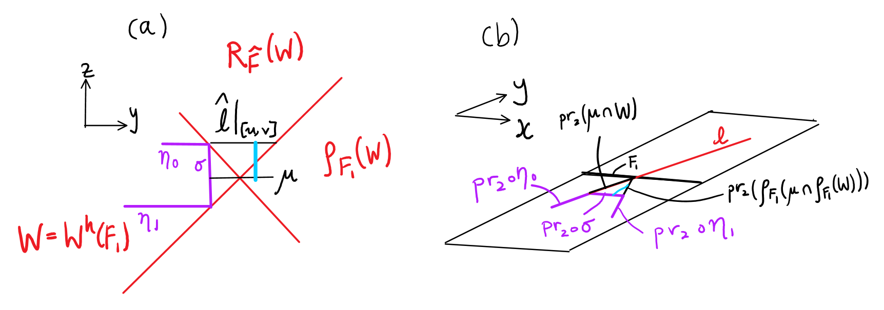
Figure 3.9: An illustration of the objects and notation used to prove Proposition 3.8(iv).

Now note that for each $r\in[u,v]$, the line segment from $\hat{\ell}(r)$ to $\mu(r)$ (which would look like the blue line segment in Figure 3.7(b)) is of length exactly $d_{\sigma}$. Hence when we “undo the unraveling” and transform $R_{\hat{F}}(\mathbf{W})$ and $\rho_{F_{1}}(\mathbf{W})$ back to $\mathbf{W}$ via the transformations $R_{\hat{F}}$ and $\rho_{F_{1}}$ respectively, these transformations send the line segment between $\hat{\ell}(r)$ and $\mu(r)$ to a piecewise-linear path—whose length is preserved—from $\hat{\beta}(r)$ to a point that projects under $\operatorname{pr}$ to $\beta(r)$. Since projecting via $\operatorname{pr}$ cannot increase the length of the piecewise-linear path, we have $\operatorname{dist}(\operatorname{pr}(\hat{\beta}(r),\beta(r)))\leq d_{\sigma}$. (The projection of the piecewise-linear path is drawn in blue in Figure 3.7(c).) ∎

The billiard trajectory $\beta$ in $\mathbf{X}$ derived from $\hat{\beta}$ in Proposition 3.8(iii) has a parallel transport map that is very closely related to that of $\hat{\beta}$, as shown in Lemma 3.6. For this reason, given a periodic billiard trajectory $\beta^{n}$ in $n$-polytope $\mathbf{X}^{n}$, we will aim to construct a beveling $\mathbf{X}^{n+1}$ of $\mathbf{X}^{n}$ and a periodic folded billiard trajectory $\beta^{n+1}$ in $\mathbf{X}^{n+1}$ such that $\beta^{n}$ is the billiard trajectory derived from $\beta^{n+1}$ via Proposition 3.8(iii). This approach will let us construct periodic billiard trajectories in convex polytopes of arbitrarily high dimension while controlling their parallel transport maps.

3.3 Origami models

As stated earlier, in order to prove Theorem 1.2, we will find a way to take a periodic billiard trajectory $\beta:[a,b]\to\mathbf{X}$ in an $n$-polytope $\mathbf{X}$ and construct some beveling $\hat{\mathbf{X}}=\operatorname{Bev}(\mathbf{X},\mathcal{F},h)$ and a periodic folded billiard trajectory $\hat{\beta}:[a,b]\to\hat{\mathbf{X}}$ such that $\beta$ is the billiard trajectory derived from $\hat{\beta}$ via Proposition 3.8(iii). Our strategy to construct $\hat{\beta}$ will be to start with the initial conditions $\hat{\beta}(a)=(\beta(a),0)$ and $\hat{\beta}^{\prime}(a)=(\beta^{\prime}(a),0)$, extend $\hat{\beta}$ forward at constant velocity until it collides with $\partial\hat{\mathbf{X}}$, extend it so that it becomes a billiard trajectory, extend forward at constant velocity until the next collision with $\partial\hat{\mathbf{X}}$, extend so that it remains a billiard trajectory, and so on until $\hat{\beta}$ has the same length as $\beta$. Of course, this is only possible if $\hat{\beta}$ only ever collides in the interiors of faces of $\hat{\mathbf{X}}$. That is, $\hat{\beta}$ must avoid the $(n-1)$-cells of $\hat{\mathbf{X}}$. Figure 3.10 illustrates several scenarios in which we may attempt to extend $\hat{\beta}:[a,t]\to\hat{\mathbf{X}}$ past a collision at $\hat{\beta}(t)$, where $\hat{\mathbf{X}}$ is the same $\hat{\mathbf{X}}$ from Figure 3.4. The extension is possible in the scenario of Figure 3.10(a) as $\hat{\beta}(t)$ lies in the interior of a face of $\hat{\mathbf{X}}$, but not in Figure 3.10(b)–(d) because $\hat{\beta}(t)$ lies on an $(n-1)$-cell of $\hat{\mathbf{X}}$.

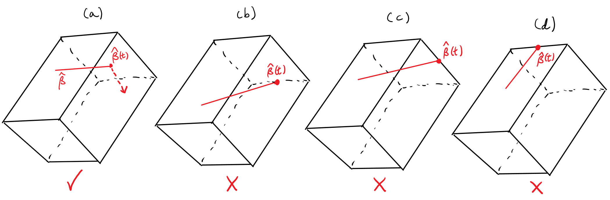
Figure 3.10: Extending a billiard trajectory $\hat{\beta}:[a,t]\to\hat{\mathbf{X}}$ past a collision at time $t$, where $\hat{\mathbf{X}}$ is the same $\hat{\mathbf{X}}$ from Figure 3.4. (a) $\hat{\beta}$ (solid red line) collides with the interior of a face of $\hat{\mathbf{X}}$, so it can be extended along the dashed line while remaining a billiard trajectory. (b)–(d): $\hat{\beta}$ collides with an edge of the polyhedron $\hat{\mathbf{X}}$, so it cannot be extended while remaining a billiard trajectory.

As we will see, the height function $h$ can be chosen carefully to avoid the scenarios in Figure 3.10(b)–(d) and ensure that $\hat{\beta}$ only ever collides in the interiors of faces of $\hat{\mathbf{X}}$. Every time $\hat{\beta}$ is extended past a collision, we wish for it to correspond to a longer and longer portion of $\beta$ under Proposition 3.8(iii), so that we can exploit Lemma 3.6 to maintain control on the parallel transport map of $\hat{\beta}$. The following definition summarizes a few of the desirable properties mentioned above.

Definition 3.10 (Origami model).

Given an $n$-polytope $\mathbf{X}$ and a billiard trajectory $\beta:[a,b]\to\mathbf{X}$ and a subset $\mathcal{F}$ of the faces of $\mathbf{X}$, we say that a partial origami model of $(\mathbf{X},\beta)$ is another pair $(\hat{\mathbf{X}},\hat{\beta})$ where $\hat{\mathbf{X}}=\operatorname{Bev}(\mathbf{X},\mathcal{F},h)$ for some $h:\mathcal{F}\to\mathbb{R}$ and $\hat{\beta}$ is the unique billiard trajectory $[a,t]\to\hat{\mathbf{X}}$ for some $t\in[a,b]$ such that the following is satisfied:

• $\hat{\beta}(a)=(\beta(a),0)$ and $\hat{\beta}^{\prime}(a)=(\beta^{\prime}(a),0)$.

• $\hat{\beta}$ is folded.

• Let $s\in[a,t]$ be the latest time such that $\hat{\beta}(s)$ lies on a horizontal segment. Then $\hat{\mathbf{X}}$ and $\hat{\beta}|_{[a,s]}$ satisfy the assumptions of Proposition 3.8(iii), and the resulting billiard trajectory in $\mathbf{X}$ is $\beta|_{[a,s]}$.

We say that this partial origam model is defined up to time $t$. When $t=b$, we say that $(\hat{\mathbf{X}},\hat{\beta})$ is a complete origami model of $(\mathbf{X},\beta)$, or simply an origami model.

Consider the following example: the $(\hat{\mathbf{X}},\hat{\beta})$ illustrated in Figure 3.3(a)–(c) is an origami model of the $(\mathbf{X},\beta)$ illustrated in Figure 3.1(a) (See Remark 3.9).

The main goal of this subsection is to prove Theorem 3.19, which stipulates some conditions under which origami models can always be constructed.

Remark 3.11.

If $(\hat{\mathbf{X}},\hat{\beta})$ is an origami model of $(\mathbf{X},\beta)$ and $a$ and $s$ are as in the definition, and $\beta|_{[a,s]}$ collides with $F_{1},\dotsc,F_{k}$ then $\hat{\beta}$ must simulate colliding at $F_{1},\dotsc,F_{k}$ and $\hat{\beta}$ must collide with every face inherited from $\mathbf{W}^{h}(F_{k})$. In particular, the parallel transport maps of $\beta|_{[a,s]}$ and $\hat{\beta}$ are related by Lemma 3.6.

In Figure 3.10(b) we see $\hat{\beta}$ collide with an $(n-1)$-cell (i.e. edge) of $\mathbf{W}^{h}(F_{1})$ at some point $\hat{\beta}(t)$. (The edges $F_{1},\dotsc,F_{4}$ of $\mathbf{X}$ are labeled in Figure 3.4.) However, if $\hat{\beta}$ is a folded billiard trajectory that simulates colliding at the same faces as $\beta$, then $\operatorname{height}(\hat{\beta}(t))$ can be predicted using Proposition 3.8(ii), so to avoid the collision of $\hat{\beta}$ with the $(n-1)$-cell of any $\mathbf{W}^{h}(F)$, we simply have to choose the height function $h$ carefully. The following definitions will help us make this choice.

Definition 3.12 (Heights in general position, isolated collisions).

Let $\beta$ be a billiard trajectory in an $n$-polytope, and let $\mathcal{F}$ be a subset of the faces of that polytope. Suppose that among the faces in $\mathcal{F}$, $\beta$ collides with $F_{1},\dotsc,F_{k}$ in that order. For each function $h:\mathcal{F}\to\mathbb{R}$, define the sequence $H_{0},H_{1},\dotsc,H_{k}$ where $H_{0}=0$ and for $1\leq i\leq k$, $H_{i}$ is defined by either of the following equivalent relations:

$$h(F_{i})=\frac{1}{2}(H_{i-1}+H_{i})\iff H_{i}=2\big{(}h(F_{i})-h(F_{i-1})+\dotsb+(-1)^{i-1}h(F_{1})\big{)}$$ (3.14)

Then we say that $h$ is in general position with respect to $\beta$ if $h(F_{i})\neq H_{i-1}$ (or equivalently, $h(F_{i})\neq H_{i}$) for all $1\leq i\leq k$. We also say that $h$ is closed with respect to $\beta$ if $H_{k}=H_{0}=0$.

Moreover, define the following key parameters:

$$\Delta(h,\beta) =\max_{1\leq i\leq k}\left\lvert h(F_{i})-H_{i}\right\rvert=\max_{1\leq i\leq k}\left\lvert h(F_{i})-H_{i-1}\right\rvert$$ (3.15)

$$H_{\max}(h,\beta) =\max_{0\leq i\leq k}H_{i}$$ (3.16)

$$H_{\min}(h,\beta) =\min_{0\leq i\leq k}H_{i}.$$ (3.17)

These parameters depend on both $h$ and $\beta$, but we will suppress this dependence when the $h$ and $\beta$ in question are clear from the context.

We say that $\beta$ has isolated collisions with respect to $h$ if every point on $\beta$ is within distance $\Delta+H_{\max}-H_{\min}$ from at most one supporting hyperplane of $\mathbf{X}$.

Remark 3.13 (Strategy to prove “niceness” of partial origami models).

The conditions of general position and isolated collisions are designed to guarantee the “niceness” of $\hat{\beta}$, a folded billiard trajectory in an origami model $(\hat{\mathbf{X}},\hat{\beta})$ of $(\mathbf{X},\beta)$. Many of the subsequent results in this section are proven using some version of the following strategy: assume that $\hat{\beta}$ comes too close to “singular features” of $\hat{\mathbf{X}}$ (such as some $(\dim\hat{\mathbf{X}}-2)$-cell). Previous results bounding the distances between points on $\hat{\beta}$ and parts of $\partial\mathbf{X}$ or $\beta$ (such as Proposition 3.8) will be chained together using the triangle inequality to show that some point on $\hat{\beta}$ will be close to multiple points on $\partial\hat{\mathbf{X}}$, which will contradict some hypothesis in the result such as isolated collisions.

Lemmas 3.14 and 3.15 lay out basic consequences of the preceding definitions.

Lemma 3.14.

Let $(\operatorname{Bev}(\mathbf{X},\mathcal{F},h),\hat{\beta})$ be a partial origami model of $(\mathbf{X},\beta)$. Then in the notation of Definition 3.12, $H_{i}$ is the height of the horizontal segments of $\hat{\beta}$ after a collision with $\mathbf{W}^{h}(F_{i})$ and, if $i\leq k-1$, before any collision with $\mathbf{W}^{h}(F_{i+1})$. Furthermore, the height of every point on $\hat{\beta}$ lies in the interval $[H_{\min},H_{\max}]$.

Proof.

The claim about $H_{i}$ can be deduced by computing with Proposition 3.8(ii), thus the rest of the lemma holds for the horizontal segments of $\hat{\beta}$. This lemma must also hold over the crease-like segments that are not the final segment, as they must lie in the convex hull of the horizontal segments. If the final segment is crease-like and simulates folding around $F_{i}$, then a similar argument implies the heights of its points range from $H_{i-1}$ to $H_{i}$, which also satisfies the lemma. ∎

Lemma 3.15.

Let $\beta$ be a billiard trajectory in an $n$-polytope, and let $\mathcal{F}$ be a subset of the faces of that polytope. Let $h:\mathcal{F}\to\mathbb{R}$ be in general position with respect to $\beta$. Then $\operatorname{im}h\subset[H_{\min}(h,\beta),H_{\max}(h,\beta)]$ and $0<\Delta(h,\beta)\leq H_{\max}(h,\beta)-H_{\min}(h,\beta)$.

Proof.

The first claim follows from Equation 3.14. The hypothesis of general position implies that $\Delta>0$. The rest follows from the fact that $\Delta$ is equal to the difference between two values in the interval $[H_{\min},H_{\max}]$. ∎

The definition of “isolated collisions” is meant to help ensure that when extending $\hat{\beta}$ as a billiard trajectory inside a partial origami model, it will only collide with the interiors of faces of $\hat{\mathbf{X}}$. Before demonstrating that, we need the following result that controls the position of the collision point $\hat{\beta}(t)$ in terms of $\beta(t)$.

Lemma 3.16.

Let $(\operatorname{Bev}(\mathbf{X},\mathcal{F},h),\hat{\beta})$ be a partial origami model of $(\mathbf{X},\beta)$ such that $\beta$ has isolated collisions with respect to $h$. Then $0<d_{\sigma}\leq\Delta$ for each crease-like segment $\sigma$ of $\hat{\beta}$, and $\operatorname{dist}(\operatorname{pr}(\hat{\beta}(s)),\beta(s))\leq\Delta$ for all times $s$ in the domain of $\hat{\beta}$.

Proof.

Let the partial origami model be defined up to time $t$. The first claim follows from Lemma 3.14.

To demonstrate the second claim, it suffices to prove the case where the final segment of $\hat{\beta}:[a,t]\to\hat{\mathbf{X}}$ is a crease-like segment $\sigma_{0}$ that simulates folding around some $F_{0}\in\mathcal{F}$, as the rest would follow from Proposition 3.8(iv). Let $\sigma_{0}$ begin at a point $\hat{\beta}(t_{0})$. Consider any $s\in[t_{0},t]$. Suppose for now that $\beta$ makes no collision during the time interval $[t_{0},s]$, except possibly with $F_{0}$. Then the proof of Proposition 3.8(iv) still works to show that $\operatorname{dist}(\operatorname{pr}(\hat{\beta}(s)),\beta(s))\leq\max_{\sigma}d_{\sigma}\leq\Delta$. Otherwise, suppose that $r\in[t_{0},s]$ is the earliest time at which $\beta$ collides with a face other than $F_{0}$, namely $F_{1}$. Then like before, the proof of Proposition 3.8(iv) would still apply to $\hat{\beta}|_{[a,r]}$ to show that $\operatorname{dist}(\operatorname{pr}(\hat{\beta}(r)),\beta(r))\leq\Delta$. But then we may apply Proposition 3.8(i) to $\sigma_{0}$ to show that $\operatorname{pr}(\hat{\beta}(r))$ lies within distance $\Delta$ from the supporting hyperplane of $F_{0}$. The triangle inequality implies that $\beta(r)$ lies within distance $2\Delta\leq\Delta+H_{\max}-H_{\min}$ (due to Lemma 3.15) from the supporting hyperplane of $F_{0}$. However, $\beta(r)\in F_{1}$, so that would contradict the hypothesis of isolated collisions. ∎

Lemma 3.17.

Let $\beta:[a,b]\to\mathbf{X}$ be a billiard trajectory in an $n$-polytope $\mathbf{X}$, and suppose that $(\operatorname{Bev}(\mathbf{X},\mathcal{F},h),\hat{\beta})$ is some partial origami model of $(\mathbf{X},\beta)$, such that $h$ is in general position with respect to $\beta$ and $\beta$ has isolated collisions with respect to $h$. Then $\hat{\beta}$ cannot end at a point that lies in the $(n-1)$-cell of $\mathbf{W}^{h}(F)$ for any $F\in\mathcal{F}$.

Proof.

Let the partial origami model be defined up to time $t$. Suppose for the sake of contradiction that $\hat{\beta}(t)$ lies in an $(n-1)$-cell of $\mathbf{W}^{h}(F)$ for some $F\in\mathcal{F}$. Two key implications are that $\operatorname{height}(\hat{\beta}(t))=h(F)$ and $\operatorname{pr}(\hat{\beta}(t))\in F$. The latter implication follows from the fact that the $(n-1)$-cell in question projects under $\operatorname{pr}$ to the supporting hyperplane of $F$, together with Lemma 3.4. There are two cases to consider, depending on whether the final segment of $\hat{\beta}$ is horizontal or crease-like; we will derive a contradiction in both cases.

• Suppose that the final segment of $\hat{\beta}$ is horizontal. Then by the definition of an origami model and Proposition 3.8(iv), $\beta(t)=\operatorname{pr}(\hat{\beta}(t))\in F$. Since $t<b$, this implies that $\beta$ collides with $F$ at time $t$. In the notation of Definition 3.12, Lemma 3.14 implies that $\operatorname{height}(\hat{\beta}(t))=H_{i-1}$ where $F_{i}=F$. However, that would contradict the hypothesis of general position.

• Suppose that the final segment of $\hat{\beta}$ is a crease-like segment $\sigma_{0}$ that simulates folding around some $F_{0}\in\mathcal{F}$. Since Proposition 3.8(i) guarantees that $\operatorname{pr}(\hat{\beta}(t))$ must lie at positive distance from the supporting hyperplane of $F_{0}$, but $\operatorname{pr}(\hat{\beta}(t))\in F$, we conclude that $F\neq F_{0}$.

  Lemma 3.16 yields $\operatorname{dist}(\operatorname{pr}(\hat{\beta}(t)),\beta(t))\leq\Delta$, thus $\beta(t)$ lies within distance $\Delta$ of the supporting hyperplane of $F$. Moreover, Proposition 3.8(i) and Lemma 3.16 imply that $\operatorname{pr}(\hat{\beta}(t))$ lies at distance $d_{\sigma_{0}}\leq\Delta$ from the supporting hyperplane of $F_{0}$. By the triangle inequality, $\beta(t)$ must lie within distance $2\Delta\leq H_{\max}-H_{\min}$ (due to Lemma 3.15) of the supporting hyperplanes of $F_{0}$ and $F$. However, this would contradict the hypothesis of isolated collisions.

∎

The preceding results can be applied to prove the following proposition, which asserts that billiard trajectories in a partial origami model have a simple geometric structure when we have general position and isolated collisions.

Proposition 3.18.

Suppose that $(\hat{\mathbf{X}}=\operatorname{Bev}(\mathbf{X},\mathcal{F},h),\hat{\beta})$ is a partial origami model of $(\mathbf{X},\beta)$, where $h$ is in general position with respect to $\beta$, and $\beta$ has isolated collisions with respect to $h$. Then the following properties hold:

1. $\hat{\beta}$ ends either in the interior of $\hat{\mathbf{X}}$ or in the interior of some face of $\hat{\mathbf{X}}$.

2. For each crease-like segment $\sigma$ of $\hat{\beta}$ that simulates folding around $F\in\mathcal{F}$, each point on ${\operatorname{pr}}\circ\sigma$ lies at distance greater than $H_{\max}-H_{\min}$ from the supporting hyperplane of any other face of $\mathbf{X}$.

3. Each crease-like segment $\sigma$ of $\hat{\beta}$ that simulates folding around $F\in\mathcal{F}$ can only intersect $\partial\hat{\mathbf{X}}$ at points in $\partial\mathbf{W}^{h}(F)$.

Proof.

Let the partial origami model be defined up to time $t$.

Statement (i): This can only be violated if $\hat{\beta}(t)$ lies in an $(n-1)$-cell of $\hat{\mathbf{X}}$. Lemma 3.17 rules out some of those possibilities, leaving only the case where $\hat{\beta}(t)\in\partial\mathbf{W}^{h}(F)\cap\partial\mathbf{W}^{h}(F^{\prime})$ for some distinct faces $F$ and $F^{\prime}$ of $\mathbf{X}$. (For instance, in Figure 3.10(c), $\hat{\beta}(t)\in\partial\mathbf{W}^{h}(F_{1})\cap\partial\mathbf{W}^{h}(F_{2})$ and in Figure 3.10(d), $\hat{\beta}(t)\in\partial\mathbf{W}^{h}(F_{1})\cap\partial\mathbf{W}^{h}(F_{3})$.)

Lemma 3.15 implies that $\operatorname{im}h\subset[H_{\min},H_{\max}]$, so applying Lemma 3.4 in conjunction with Lemma 3.14 tells us that $\operatorname{pr}(\hat{\beta}(t))$ would have to lie within distance $H_{\max}-H_{\min}$ from the supporting hyperplanes of $F$ and $F^{\prime}$. We would also have $\operatorname{dist}(\operatorname{pr}(\hat{\beta}(t)),\beta(t))\leq\Delta$, due to Lemma 3.16. The triangle inequality would then imply that $\beta(t)$ lies within distance $\Delta+H_{\max}-H_{\min}$ of both of those supporting hyperplanes, contradicting the hypothesis of isolated collisions.

Statement (ii): Let $\sigma$ be a crease-like segment of $\hat{\beta}$ that simulates folding around $F$. Suppose that some point $y=\operatorname{pr}(\hat{\beta}(s))\in\operatorname{pr}(\sigma)$ is within distance $H_{\max}-H_{\min}$ from the supporting hyperplane of some $F^{\prime}$; we will prove that $F^{\prime}=F$. By Proposition 3.8(i) and Lemma 3.16, $y$ is also within distance $\Delta$ from the supporting hyperplane of $F$. By applying the triangle inequality together with Lemma 3.16, we find that $\beta(t)$ lies within distance $2\Delta\leq\Delta+H_{\max}-H_{\min}$ (due to Lemma 3.15) from the supporting hyperplane of $F$ and within distance $\Delta+H_{\max}-H_{\min}$ from the supporting hyperplane of $F^{\prime}$. Thus the hypothesis of isolated collisions implies that $F^{\prime}=F$.

Statement (iii): Suppose that a crease-like segment $\sigma$ intersects $\partial\hat{\mathbf{X}}$ at some point $y$. Then $y\in\partial\mathbf{W}^{h}(F)$ for some face $F$ of $\mathbf{X}$. As shown in Statement (i), Lemma 3.4 and Lemma 3.14 would require $\operatorname{pr}(y)$ to lie within distance $H_{\max}-H_{\min}$ of the supporting hyperplane of $F$. Hence Statement (ii) would require that $\sigma$ simulate folding around $F$. ∎

The properties of beveling and partial origami models that we have proved so far will help us prove our main technical theorem, which we will use to construct origami models:

Theorem 3.19 (Construction of origami model).

Let $\mathbf{X}$ be an $n$-polytope with a billiard trajectory $\beta:[a,b]\to\mathbf{X}$ that collides with each face at most once. Let $\mathcal{F}$ be a subset of the faces of $\mathbf{X}$, and let $h:\mathcal{F}\to\mathbb{R}$ be in general position and closed with respect to $\beta$, such that $\beta$ also has isolated collisions with respect to $h$. In addition, make the following assumptions:

• $(\beta|_{[a,c]},0)\subset\hat{\mathbf{X}}=\operatorname{Bev}(\mathbf{X},\mathcal{F},h)$ for some $c>a$.

• $\beta(b)$ lies at a distance greater than $2\Delta$ from the supporting hyperplane of every face that $\beta$ collides with.

Then $(\mathbf{X},\beta)$ has an origami model $(\hat{\mathbf{X}},\hat{\beta})$ such that $\hat{\beta}(b)=(\beta(b),0)$ and $\hat{\beta}^{\prime}(b)=(\beta^{\prime}(b),0)$. Moreover, $\hat{\beta}$ collides with each face of $\hat{\mathbf{X}}$ at most once.

Proof.

Let $\beta$ collide with the faces $F_{1},\dotsc,F_{k}$. For each given value of $t\in[a,b]$, there may exist a billiard trajectory $\hat{\beta}:[a,t]\to\hat{\mathbf{X}}$ with $\hat{\beta}(a)=(\beta(a),0)$ and $\hat{\beta}^{\prime}(a)=(\beta^{\prime}(a),0)$. If it exists, then it is unique. In fact, $\hat{\beta}$ should exist as a billiard trajectory for $t=c$, by a hypothesis of the theorem. Thus $(\hat{\mathbf{X}},\hat{\beta})$ is a partial origami model of $(\mathbf{X},\beta)$ that is defined up to time $c$. Intuitively, our strategy to prove the theorem will be to start with this partial origami model and extend $\hat{\beta}$ to longer and longer billiard trajectories $\hat{\beta}:[a,t]\to\hat{\mathbf{X}}$ such that $(\hat{\mathbf{X}},\hat{\beta})$ continues to be a partial origami model of $(\mathbf{X},\beta)$, which is defined up to greater and greater values of time until it is defined up to time $b$.

Now suppose that $(\hat{\mathbf{X}},\hat{\beta})$ is a partial origami model of $(\mathbf{X},\beta)$ that is defined up to time $t$. Whenever $\hat{\beta}(t)$ and $\beta(t)$ both lie in the interiors of $\hat{\mathbf{X}}$ and $\mathbf{X}$ respectively, $\hat{\beta}$ can be extended along its final segment while preserving the definition of a partial origami model. Thus we only have to check that continued extension is possible when $\hat{\beta}(t)\in\partial\hat{\mathbf{X}}$ or $\beta(t)\in\partial\mathbf{X}$.

First suppose that $\beta(t)$ is the point of collision with $F_{i}$. There are two cases depending on whether $\hat{\beta}(t)$ lies on a horizontal segment or on a crease-like segment. We will perform the extension in both cases.

1. Suppose that $\hat{\beta}(t)$ lies in the interior or at the ending point of a horizontal segment. Then the definition of a partial origami model and Proposition 3.8(iv) imply that $\operatorname{pr}(\hat{\beta}(t))=\beta(t)$. We must have $F_{i}\notin\mathcal{F}$, otherwise $\hat{\beta}(t)$ would have to lie on an $(n-1)$-cell of $\mathbf{W}^{h}(F_{i})$, contradicting Lemma 3.17. By the definition of the beveling $\operatorname{Bev}(\mathbf{X},\mathcal{F},h)$, $\hat{\beta}(t)\in\partial\mathbf{W}^{h}(F_{i})$. By Proposition 3.18(i), $\hat{\beta}(t)$ lies in the interior of a face of $\hat{\mathbf{X}}$. Therefore $\hat{\beta}$ can be extended slightly into a uniquely determined billiard trajectory $\alpha:[a,t+\epsilon]\to\hat{\mathbf{X}}$ such that $(\hat{\mathbf{X}},\alpha)$ is a partial origami model of $(\mathbf{X},\beta)$, defined up to time $t+\epsilon$. (Near the extension, $\hat{\beta}$ and $\beta$ would look like the $\hat{\beta}$ and ${\operatorname{pr}}\circ\hat{\beta}$ depicted in Figure 3.2(b).)

2. Suppose that $\hat{\beta}(t)$ lies on a crease-like segment $\sigma$. It would suffice to prove that $\hat{\beta}(t)$ lies in the interior of $\hat{\mathbf{X}}$, as that would allow us to extend $\hat{\beta}$ slightly along its final crease-like segment, without introducing new collisions, into a billiard trajectory $\alpha:[a,t+\epsilon]\to\hat{\mathbf{X}}$ for some $0<\epsilon<b-t$. Moreover, for sufficiently small $\epsilon$, we can verify that $(\hat{\mathbf{X}},\alpha)$ is a partial origami model of $(\mathbf{X},\beta)$, defined up to time $t+\epsilon$.

   We may apply Lemma 3.16 to deduce that $\operatorname{pr}(\hat{\beta}(t))$ lies within distance $\Delta\leq H_{\max}-H_{\min}$ (due to Lemma 3.15) from $\beta(t)\in F_{i}$. Consequently, Proposition 3.18(ii) requires that $\sigma$ simulates folding around $F_{i}$—that is, $F_{i}\in\mathcal{F}$. Examining the proof of Proposition 3.8(iv) reveals that since $\beta(t)$ is a collision point on $F_{i}\in\mathcal{F}$, $\hat{\beta}(t)$ must lie in the interior of $\mathbf{W}^{h}(F_{i})$. (For example, in the context of Figure 3.8, if $\beta(t)=x_{1}$ then $\hat{\beta}$ would consist of $\eta_{0}$ and the first half of $\sigma$, ending at $\hat{\beta}(t)$ which is the midpoint of $\sigma$.) Together with Proposition 3.18(iii), this implies that $\hat{\beta}(t)$ lies in the interior of $\hat{\mathbf{X}}$.

Next, suppose that $\beta(t)$ lies in the interior of $\mathbf{X}$ but that $\hat{\beta}(t)\in\partial\hat{\mathbf{X}}$. In particular, Proposition 3.18(i) guarantees that $\hat{\beta}(t)$ lies in the interior of a face of $\hat{\mathbf{X}}$ that is inherited from $\mathbf{W}^{h}(F)$ for some face $F$ of $\mathbf{X}$. Then we can extend $\hat{\beta}$ slightly to a billiard trajectory $\alpha:[a,t+\epsilon]\to\hat{\mathbf{X}}$ for some $\epsilon\in(0,b-t)$. We will prove that for sufficiently small $\epsilon$, $(\hat{\mathbf{X}},\alpha)$ is a partial origami model of $(\mathbf{X},\beta)$ that is defined up to time $t+\epsilon$.

If $F\notin\mathcal{F}$, then $\operatorname{pr}(\hat{\beta}(t))$ lies in the supporting hyperplane of $F$. The final segment of $\hat{\beta}$ has to be horizontal, otherwise Proposition 3.18(ii) would imply that the final segment simulates folding around $F$, but that would contradict our assumption that $F\notin\mathcal{F}$. Then Proposition 3.8(iv) implies that $\beta(t)=\operatorname{pr}(\hat{\beta}(t))$. Hence we are in case (1) that has been handled earlier.

Otherwise $F\in\mathcal{F}$. Suppose that the final segment of $\hat{\beta}$ is horizontal. Then Proposition 3.8(iv) implies that $\operatorname{pr}(\hat{\beta}(t))=\beta(t)$. Therefore $\hat{\beta}$ is extended to $\alpha$ along a crease-like segment which is disregarded by the definition of a partial origami model. Thus $(\hat{\mathbf{X}},\alpha)$ is a partial origami model of $(\mathbf{X},\beta)$.

On the other hand, suppose that $F\in\mathcal{F}$ and the final segment $\sigma$ of $\hat{\beta}$ is crease-like. Proposition 3.18(iii) implies that $\sigma$ must simulate folding around $F$ and in particular it must start from one of the faces inherited from $\mathbf{W}^{h}(F)$ and end at the other. Thus if we extend $\hat{\beta}$ slightly along a new segment $\eta_{1}$ into a billiard trajectory $\alpha:[a,t+\epsilon]\to\hat{\mathbf{X}}$ for some $\epsilon\in(0,b-t)$, $\alpha$ remains a folded billiard trajectory.

Now we verify that $\alpha$ satisfies the assumption of Proposition 3.8(iii). Let $\eta_{0}$ be the segment of $\hat{\beta}$ preceding $\sigma$, and let $\hat{\beta}(s)$ be the point of collision of $\hat{\beta}$ between $\eta_{0}$ and $\sigma$. Applying Proposition 3.8(iii)–(iv) to $\hat{\beta}|_{[a,s^{\prime}]}$ for $s^{\prime}\leq s$ implies that $\beta(s)=\operatorname{pr}(\hat{\beta}(s))$ and $\beta^{\prime}(s)=\lim_{r\to s^{-}}\operatorname{pr}(\hat{\beta}^{\prime}(r))$. It suffices to verify the assumption of Proposition 3.8(iii) for $\eta_{0}$ and $\eta_{1}$. By the first part of Proposition 3.8(iii), ${\operatorname{pr}}\circ\eta_{0}$ and ${\operatorname{pr}}\circ\eta_{1}$ extend into lines that intersect the supporting hyperplane of $F$ at the same point $x$. To show that $x$ lies in the interior of $F$, it suffices to show that as $\beta$ continues past time $s$, the first face $F_{i}$ that it collides with must actually be $F$. It must make such a collision and it should occur at a time $t_{i}\leq t$, otherwise a contradiction would arise from the fact that $\hat{\beta}$ and $\beta$ travel at the same speed, thus $\beta$ would collide with $F$ first before time $t$. (This can be deduced from the unraveling of the parts of $\hat{\beta}$ and $\beta$ from $\eta_{0}$ and ${\operatorname{pr}}\circ\eta_{0}$ onwards; in Figure 3.7, our assertion can be interpreted as saying that $\ell$ must hit $F_{1}$ before $\hat{\ell}$ finishes traversing $\hat{\ell}_{1}$.) By Lemma 3.16, $\operatorname{dist}(\operatorname{pr}(\hat{\beta}(t_{i})),\beta(t_{i}))\leq\Delta$. In other words, ${\operatorname{pr}}\circ\sigma$ is within distance $\Delta$ from the supporting hyperplane of $F_{i}$. Lemma 3.15 and Proposition 3.18(ii) imply that $F_{i}=F$. Therefore $x$ is actually a point of collision of $\beta$, which must lie in the interior of $F$.

This means that $\beta$ continues past $\beta(s)$ to collide with $F_{i}$ at $x$. It then reflects as a billiard trajectory should and, for similar reasons as above, it cannot make any more collisions until time $t$. Moreover, recall our assumption that $\beta(t)$ lies in the interior of $\mathbf{X}$. Therefore it can be verified that $(\hat{\mathbf{X}},\alpha)$ is a partial origami model of $(\mathbf{X},\beta)$. (Near the extension, $\hat{\beta}$ and $\beta$ would look like the $\hat{\beta}$ and ${\operatorname{pr}}\circ\hat{\beta}$ depicted in Figure 3.2(a).)

Therefore we can eventually extend to get a complete origami model $(\hat{\mathbf{X}},\hat{\beta})$ of $(\mathbf{X},\beta)$. Now we must show that $\hat{\beta}(b)=(\beta(b),0)$ and $\hat{\beta}^{\prime}(b)=(\beta^{\prime}(b),0)$. By Proposition 3.8(iv), Lemma 3.14 and our hypothesis that $h$ is closed with respect to $\beta$, it suffices to show that the final segment of $\hat{\beta}$ is horizontal. Indeed, Lemma 3.16 implies that $\operatorname{dist}(\operatorname{pr}(\hat{\beta}(b)),\beta(b))\leq\Delta$. If the final segment of $\hat{\beta}$ was crease-like and simulated folding around $F_{i}$, then Proposition 3.8(i) and Lemma 3.16 would imply that $\operatorname{pr}(\hat{\beta}(b))$ lies within distance $\Delta$ of the supporting hyperplane of $F_{i}$. The triangle inequality would then imply that $\beta(b)$ lies within distance $2\Delta$ of the supporting hyperplane of $F_{i}$, contradicting one of the assumptions in the theorem statement.

By the definition of a complete origami model and the fact that $\hat{\beta}$’s final segment is horizontal, $\hat{\beta}$ must simulate colliding at $F_{1},\dotsc,F_{k}$, which is a non-repeating sequence of faces, so $\hat{\beta}$ never collides twice with the same face of $\hat{\mathbf{X}}$. ∎

The preceding theorem helps us construct origami models $(\hat{\mathbf{X}},\hat{\beta})$ of $(\mathbf{X},\beta)$. On top of that, since we are interested in constructing simple closed geodesics and simple stable figure-eights, the following lemma gives some conditions which guarantee that when $\beta$ is simple, $\hat{\beta}$ will also be simple.

Lemma 3.20.

Suppose that $(\operatorname{Bev}(\mathbf{X},\mathcal{F},h),\hat{\beta})$ is an origami model of $(\mathbf{X},\beta)$, where $\beta$ is simple and collides with each face of $\mathbf{X}$ at most once. Assume also that $h$ is in general position with respect to $\beta$, and that $\beta$ has isolated collisions with respect to $h$. For each face $F$ of $\mathbf{X}$ that $\beta$ collides with, let $\beta_{F}$ be the intersection of $\operatorname{im}\beta$ with the neighbourhood of radius $\Delta(h,\beta)$ around the supporting hyperplane of $F$. Assume that each $\beta_{F}$ only intersects the two segments of $\beta$ that come immediately before and after the collision at $F$. Then $\hat{\beta}$ is also simple.

Proof.

We will assume that $\beta(a)\neq\beta(b)$; the proof will be similar for the other case. Suppose for the sake of contradiction that $\hat{\beta}$ self-intersects. Then $\hat{\beta}$ must have two non-adjacent segments that intersect each other, where two segments of $\hat{\beta}$ are considered to be adjacent if $\hat{\beta}$ traverses one of them immediately after the other. They cannot both be horizontal segments, otherwise by the definition of an origami model and Proposition 3.8(iii) they would project to subsets of non-adjacent segments of $\beta$, which cannot intersect since $\beta$ is simple.

They also cannot both be crease-like segments. Otherwise, they would simulate folding around two distinct $F_{i},F_{j}\in\mathcal{F}$—where $\beta$ collides with $F_{1},\dotsc,F_{k}$—because $\beta$ collides with each of those faces exactly once, and $\hat{\beta}$ simulates colliding at the same faces in the same order. If the crease-like segments intersect at $x$, then Proposition 3.8(i) and Lemma 3.16 would require $\operatorname{pr}(x)$ to lie within distance $\Delta\leq H_{\max}-H_{\min}$ (due to Lemma 3.15) of the supporting hyperplanes of both $F_{i}$ and $F_{j}$, but that would contradict Proposition 3.18(ii).

Hence it remains to rule out the case where some crease-like segment $\sigma$ intersects a non-adjacent horizontal segment $\eta$. Let the $\sigma$ simulate folding around $F_{i}$. If $\sigma$ and $\eta$ intersect at some point $x$, then like before, $\operatorname{pr}(x)$ would have to lie within distance $\Delta$ of the supporting hyperplane of $F_{i}$, thus $\operatorname{pr}(x)\in\beta_{F_{i}}$. However, since $x$ also lies on a horizontal segment, Proposition 3.8(iv) guarantees that $\operatorname{pr}(x)$ lies on a segment of $\beta$, which cannot be one of the segments that come immediately before or after the collision at $F_{i}$, otherwise $\sigma$ would have to be adjacent to $\eta$. This contradicts our hypothesis on $\beta_{F_{i}}$. ∎

3.4 Construction of index-zero closed geodesics in convex hypersurfaces

Let us apply bevelings and origami models to construct index-zero closed geodesics in convex hypersurfaces. First we derive a corollary of our earlier results:

Corollary 3.21.

For every integer $n\geq 2$, there exists an $n$-polytope $X^{n}$ that has a simple and periodic billiard trajectory $\beta^{n}:[a,b]\to\mathbf{X}^{n}$ whose parallel transport map is $1\oplus(-I_{n-1})$, with respect to the decomposition $\mathbb{R}^{n}=\operatorname{span}\{(\beta^{n})^{\prime}(a)\}\oplus\operatorname{span}\{(\beta^{n})^{\prime}(a)\}^{\perp}$. Moreover, the number of collisions of $\beta^{n}$ has opposite parity from $n$, and $\beta^{n}$ collides with each face of $\mathbf{X}^{n}$ at most once.

Proof.

We will construct $\mathbf{X}^{n}$ and $\beta^{n}$ inductively using Theorem 3.19 and prove the necessary properties by induction. For $n=2$, we can choose $X^{2}$ and $\beta^{2}$ to be the $\mathbf{X}$ and $\beta$ from Figure 3.1(a).

For any $n\geq 2$, assume that the statement of the corollary holds for some $\mathbf{X}^{n}$ and $\beta^{n}$. Let $\mathcal{F}=\{F_{1},F_{2},F_{3}\}$ be any set of 3 faces of $\mathbf{X}^{n}$ that $\beta^{n}$ collides with, indexed in the order of collision. For some $\delta>0$, define the function $h:\mathcal{F}\to\mathbb{R}$ by $h(F_{1})=\delta$, $h(F_{2})=0$ and $h(F_{3})=-\delta$. With these settings, one can compute $\Delta(h,\beta)=2\delta$, $H_{\max}(h,\beta)=2\delta$ and $H_{\min}(h,\beta)=-2\delta$. Hence $\Delta+H_{\max}-H_{\min}=6\delta$. Some geometry shows that we can choose $\delta$ small enough such that the hypotheses of Theorem 3.19 are satisfied. Since $\beta^{n}$ is simple and it collides with each face of $\mathbf{X}$ at most once, we can also choose $\delta$ small enough to satisfy the hypotheses of Lemma 3.20. Consequently we get an origami model $(\mathbf{X}^{n+1}=\operatorname{Bev}(\mathbf{X},\mathcal{F},h),\beta^{n+1})$ of $(X^{n},\beta^{n})$ such that $\beta^{n+1}$ is periodic and simple, and it collides with each faces of $\mathbf{X}^{n+1}$ at most once. (As an example, for $n=2$, we can choose $\delta=0.05$ to get Figures 3.1 and 3.3.)

By applying Lemma 3.6 along the lines of Remark 3.11, the parallel transport map of $\beta^{n+1}$ is $1\oplus(-I_{n-1})\oplus(-1)^{3}=1\oplus(-I_{n})$ with respect to the required decomposition of $\mathbb{R}^{n+1}$. Moreover, the number of collisions of $\beta^{n+1}$ will be 3 more than that of $\beta^{n}$, and will have opposite parity to $n+1$. ∎

Now we are ready to prove Theorem 1.2.

Proof of Theorem 1.2.

For each odd integer $n\geq 3$, let $X^{n}$ and $\beta^{n}$ be the $n$-polytope and periodic billiard trajectory produced in Corollary 3.21. By that corollary, $\beta^{n}$ has an even number of collisions, and is a simple closed curve. Hence it corresponds to a simple closed geodesic $\gamma$ in $\mathcal{D}_{\mathrm{}}\mathbf{X}^{n}$. The parallel transport map is $1\oplus(-I_{n-1})$ with respect to the decomposition of $\mathbb{R}^{n}$ given by a tangent vector of $\beta^{n}$ and its orthogonal complement, which implies that a tubular neighbourhood of $\gamma$ is in fact an $n$-dimensional maximally-twisted tube $T$. As explained in Section 1.1.1, the flat metric of $T$ means that $\gamma$ has index zero. $\gamma$ is also non-degenerate by Lemma 3.1.

Since $\gamma$ is simple and it is also a stable geodesic bouquet with one loop, we may apply [Che22, Propositions 4.7 and 4.8] to prove the desired result. ∎

Remark 3.22 (Parity sequences for origami models).

To prove Corollary 3.21 we iterated the construction of an origami model, each time folding along 3 faces. Each iteration increases the dimension of the space acted on by the parallel transport map by 1, and folding along an odd number of faces is important as it ensures that the parallel transport maps acts by negation on that additional dimension. As a result, in the odd dimensions we have maximally-twisted tubes. Folding by an even number of faces would yield a parallel transport map that fixes some vector orthogonal to the billiard trajectory, potentially giving a parallel vector field along the corresponding closed geodesic. This could give rise to a length-decreasing variation of the corresponding geodesic after smoothing the double of the polytope to a positively-curved manifold, along the lines of the proof of Synge’s theorem [Syn36]. Hence in the proof of Corollary 3.21, the parity of the number of collisions of the initial billiard trajectory $\beta^{2}$, followed by the parities of the number of faces we fold along to get $\beta^{n}$ is “odd, odd$,\dotsc$, odd”—a sequence of $n-1$ odd numbers. The number of collisions in the final billiard trajectory is the sum of odd numbers, which is even when $n$ is odd but odd otherwise. When the sum is even, the billiard trajectory corresponds to a closed geodesic that helps us to prove Theorem 1.2. This does not occur when $n$ is even, so our construction does not contradict Synge’s theorem.

The above discussion suggests that applying the construction of origami models may require careful choices on the parity of the number of collisions of the initial billiard trajectory and the number of faces we fold along. We wish to fold along an odd number of faces whenever possible to “add twisting” and obstruct the existence of parallel vector fields along the corresponding closed geodesic. However, we need these numbers to add up to an overall even number of collisions in the final billiard trajectory, so that it corresponds to a geodesic loop in the double. As we apply this construction to construct stable figure-eights in Riemannian spheres of every dimension, the latter constraint may sometimes force us to fold along an even number of faces. In such a situation, we will explain how to mitigate the problem by choosing the right dimensions to fold along an even number of faces.

4 Construction of Stable Figure-eights

From the discussion in Section 2, we can reduce Theorem 1.1 to the construction of a 3-polytope, 4-polytope, and 5-polytope whose doubles contain stable figure-eights. We will prove those cases in this section. Our arguments will frequently start with a billiard loop in a convex polygon and then apply the origami model construction iteratively so that the resulting billiard loop corresponds to a geodesic loop in the final stable figure-eight.

As explained in Section 1.1.2, each geodesic loop $\gamma$ in a stationary geodesic bouquet can be associated with a subspace of the tangent space at the basepoint called the parallel defect kernel, denoted by $\ker D_{\gamma}$ and defined in [Che22, Definition 3.2]. The bouquet is stable if the parallel defect kernels of all of its loops intersect at a point and the curvature near the bouquet is sufficiently small. When we derive the loops of the bouquet from origami models, then their parallel defect kernels have a very specific and convenient form that can be computed using the following pair of lemmas.

Lemma 4.1.

Consider a convex polygon $\mathbf{X}\subset\mathbb{R}^{2}$ with a billiard trajectory $\beta:[a,b]\to\mathbf{X}$. Then after canonically identifying tangent spaces with $\mathbb{R}^{2}$, the parallel transport map $T_{\beta(a)}\mathbf{X}\to T_{\beta(b)}\mathbf{X}$ is the reflection in $O(2)$ that sends $\beta^{\prime}(a)$ to $\beta^{\prime}(b)$ if $\beta$ collides an odd number of times, and it is the rotation in $SO(2)$ that sends $\beta^{\prime}(a)$ to $\beta^{\prime}(b)$ if $\beta$ collides an even number of times.

Proof.

The reflection and rotation stated in the lemma are the only possibilities given that the parallel transport maps are products of reflections in $O(2)$ that send the velocity vector of the trajectory before each collision to the velocity vector right after. The determinant of the parallel transport map is determined by the parity of the number of reflection factors. ∎

Lemma 4.2.

Consider a convex polygon $\mathbf{X}^{2}\subset\mathbb{R}^{2}$ with a billiard loop $\beta^{2}:[0,1]\to\mathbf{X}$ based at $p$ such that $(\beta^{2})^{\prime}(0)$ is linearly independent from $v=(\beta^{2})^{\prime}(1)$. Consider a sequence $(\mathbf{X}^{3},\beta^{3}),(\mathbf{X}^{4},\beta^{4}),\dotsc,(\mathbf{X}^{n},\beta^{n})$ in which $(\mathbf{X}^{m+1}=\operatorname{Bev}(\mathbf{X}^{m},\mathcal{F}_{m},h_{m}),\beta^{m+1})$ is an origami model of $(\mathbf{X}^{m},\beta^{m})$ for $2\leq m\leq n-1$, and suppose that the following conditions hold:

• $\beta^{m}(1)=(p,0,\dotsc,0)$ and $(\beta^{m})^{\prime}(1)=(v,0,\dotsc,0)$ for all $m$.

• Each $\beta^{m}$ collides with every face in $\mathcal{F}_{m}$.

• Let $c_{m}$ be the number of collisions of $\beta^{m}$, and suppose that $c_{n}$ is even, so that $\beta^{n}$ corresponds to a geodesic loop $\gamma$ in $\mathcal{D}_{\mathrm{}}\mathbf{X}^{n}$.

Then under the identification of $T_{\gamma(0)}\mathcal{D}_{\mathrm{}}\mathbf{X}^{n}$ with $\mathbb{R}^{n}$ induced by the quotient map $\mathcal{D}_{\mathrm{}}\mathbf{X}^{n}\to\mathbf{X}^{n}\subset\mathbb{R}^{n}$,

$$\ker D_{\gamma}=V_{2}\oplus V_{3}\oplus\dotsb\oplus V_{n},$$ (4.1)

where $V_{2}=\operatorname{span}\{(\beta^{n})^{\prime}(0)-(-1)^{c_{2}}(\beta^{n})^{\prime}(1)\}$ and for each $m\geq 3$, $V_{m}$ is the span of the $m^{\text{th}}$ standard basis vector of $\mathbb{R}^{n}$ if $\left\lvert\mathcal{F}_{m-1}\right\rvert$ is even, and $V_{m}=\{0\}$ if $\left\lvert\mathcal{F}_{m-1}\right\rvert$ is odd.

Proof.

If $P_{m}:\mathbb{R}^{m}\to\mathbb{R}^{m}$ is the parallel transport map of $\beta^{m}$ (after canonically identifying tangent spaces with the ambient Euclidean space), then Remark 3.11 and Lemma 3.6 imply that

$$P_{n}=\underbrace{P_{2}}_{P_{n}|_{W}}\oplus\underbrace{(-1)^{\left\lvert\mathcal{F}_{2}\right\rvert}\oplus(-1)^{\left\lvert\mathcal{F}_{3}\right\rvert}\oplus\dotsb\oplus(-1)^{\left\lvert\mathcal{F}_{n-1}\right\rvert}}_{P_{n}|_{W^{\perp}}},$$ (4.2)

where $W=\operatorname{span}\{(\beta^{n})^{\prime}(0),(\beta^{n})^{\prime}(1)\}=\mathbb{R}^{2}\times\{(0,\dotsc,0)\}$ is an invariant subspace of $P_{n}$. The form of $V_{2}$ comes from the corresponding direct summand in Proposition 3.5 from [Che22], after considering Lemma 4.1.

For $m\geq 3$, $V_{m}$ is obtained by computing the eigenspace of $P_{n}|_{W^{\perp}}$ that corresponds to the eigenvalue 1, according to [Che22, Proposition 3.5]. ∎

Lemma 4.2 shows that if we wish to iterate the origami model construction to produce geodesic loops with parallel defect kernels of low dimension, then it is important to carefully choose the parities of several integers, reminiscent of Remark 3.22. For instance, the parity of $c_{2}$ controls $V_{2}$. We would also prefer most origami models to fold along an odd number of faces so that as many of the $V_{m}$’s are 0-dimensional as possible; but we also need $c_{n}=c_{2}+\left\lvert\mathcal{F}_{2}\right\rvert+\dotsb+\left\lvert\mathcal{F}_{n-1}\right\rvert$ to be even so that the resulting billiard loop $\beta^{n}$ corresponds to a geodesic loop in $\mathcal{D}_{\mathrm{}}\mathbf{X}^{n}$. Hence we should pay attention to the parity sequence of a series of origami model constructions, by which we mean the sequence of parities of $c_{2},\left\lvert\mathcal{F}_{2}\right\rvert,\dotsc,\left\lvert\mathcal{F}_{n-1}\right\rvert$.

Let us proceed to perform the main construction for the 3-dimensional case of Theorem 1.1.

Proposition 4.3.

There exists a convex polyhedron $\mathbf{X}^{3}\subset\mathbb{R}^{3}$ and simple billiard loops $\alpha^{3},\beta^{3}$ in $\mathbf{X}^{3}$ that correspond to two geodesic loops of a simple and irreducible stable figure-eight in $\mathcal{D}_{\mathrm{}}\mathbf{X}^{3}$. Moreover, $\alpha^{3}$ only intersects $\beta^{3}$ at their common basepoint.

Proof.

We want to find such $\alpha^{3},\beta^{3}$ that correspond to geodesic loops $\gamma_{1},\gamma_{2}$. By applying Corollary 3.4 from [Che22] to the smooth (flat) part of $\mathcal{D}_{\mathrm{}}\mathbf{X}^{3}$, we need $\ker D_{\gamma_{1}}\cap\ker D_{\gamma_{2}}=\{0\}$. However this means that we need $\dim\ker D_{\gamma_{i}}\leq 1$ for some $i$. We will in fact construct $\mathbf{X}^{3}$ and $\gamma_{1},\gamma_{2}$ such that $\dim\ker D_{\gamma_{1}}=\dim\ker D_{\gamma_{2}}=1$. To obtain each geodesic loop, we will apply the origami model construction once using the parity sequence “odd, odd”.

Now consider the square $\mathbf{Y}^{2}=[-2,0]\times[-1,1]\subset\mathbb{R}^{2}$, whose “faces” (edges) are $F_{0}$, $F_{1}$, $F_{2}$ and $F_{3}$, listed in counterclockwise order from $F_{0}$ which contains the origin. Let $\alpha^{2}:[0,1]\to\mathbf{Y}^{2}$ be the billiard trajectory that starts from the origin, collides at the points $(-1,1)$, $(-2,0)$ and $(-1,-1)$ in order, and then returns to the origin (see Figure 4.1(a)). Let $\mathcal{F}=\{F_{1},F_{2},F_{3}\}$ and $h:\mathcal{F}\to\mathbb{R}$ be the function defined by $h(F_{1})=\delta$, $h(F_{2})=0$ and $h(F_{3})=-\delta$, where $\delta=0.08$. As in the proof of Corollary 3.21, $\Delta(h,\alpha^{2})+H_{\max}(h,\alpha^{2})-H_{\min}(h,\alpha^{2})=6\delta<0.5$. Thus the hypotheses of Theorem 3.19 are satisfied, which guarantees the existence of an origami model $(\mathbf{Y}^{3}=\operatorname{Bev}(\mathbf{Y}^{2},\mathcal{F},h),\alpha^{3})$ of $(\mathbf{Y}^{2},\alpha^{2})$. Figure 4.1(b)–(d) depicts $\mathbf{Y}^{3}$ and $\alpha^{3}$ from three different points of view, but for a larger value of $\delta$ to emphasize the important features. In particular, $\alpha^{3}(1)=(\alpha^{2}(1),0)=\alpha^{3}(0)$ and $(\alpha^{3})^{\prime}(1)=((\alpha^{2})^{\prime}(1),0)$.

Now let $\rho\in SO(3)$ be the rotation by angle $\pi$ about the line spanned by the vector $(0,1,1)$. One can verify that $\mathbf{X}^{3}=\mathbf{Y}^{3}\cup\rho(\mathbf{Y}^{3})$ is a convex polyhedron. As $\alpha^{3}$ is a billiard loop in $\mathbf{X}^{3}$ with an even number of collisions, it corresponds to a geodesic loop $\gamma_{1}$ in $\mathcal{D}_{\mathrm{}}\mathbf{X}^{3}$. Similarly, $\beta^{3}=\rho\circ\alpha^{3}$ also corresponds to a geodesic loop $\gamma_{2}$ in $\mathcal{D}_{\mathrm{}}\mathbf{X}^{3}$ that shares the same basepoint $p$ as $\gamma_{1}$. $\mathbf{X}^{3}$, $\alpha^{3}$ and $\beta^{3}$ are illustrated in Figure 4.1(f).

It can be verified that $\gamma_{1}$ and $\gamma_{2}$ form an irreducible stationary geodesic bouquet $G^{3}$ in $\mathcal{D}_{\mathrm{}}\mathbf{X}^{3}$ that is based at $p$. By [Che22, Corollary 3.4], it remains to show that $\ker D_{\gamma_{1}}\cap\ker D_{\gamma_{2}}=\{0\}$. Lemma 4.2 implies that $\ker D_{\gamma_{1}}$ is the $y$-axis, under the identification of $T_{p}\mathcal{D}_{\mathrm{}}\mathbf{X}^{3}$ with $\mathbb{R}^{3}$ induced by the quotient map $\mathcal{D}_{\mathrm{}}\mathbf{X}^{3}\to\mathbf{X}^{3}\subset\mathbb{R}^{3}$. Due to the rotation by $\rho$, $\ker D_{\gamma_{2}}$ is the $z$-axis, which intersects $\ker D_{\gamma_{1}}$ only at the origin.

Lemma 3.20 implies that $\alpha^{3}$ and $\beta^{3}$ are simple. By construction, they intersect only at their common basepoint. As a result, $G^{3}$ is also simple. ∎

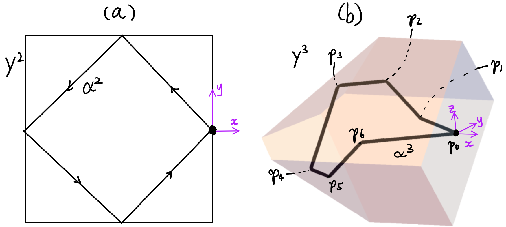
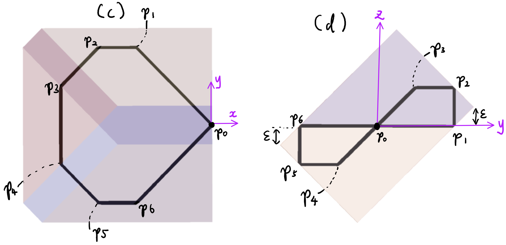
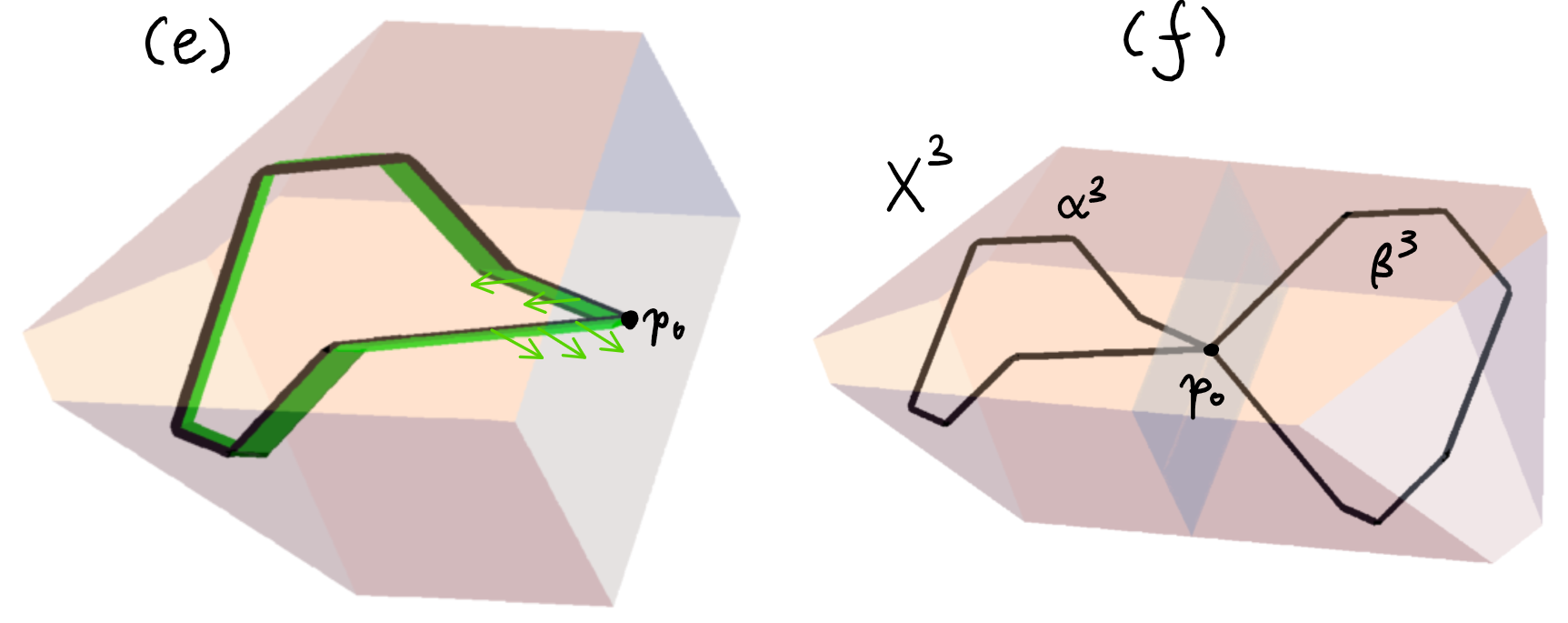
Figure 4.1: Various stages from the construction of a stable figure-eight in the proof of Proposition 4.3, illustrated for a larger value of $\delta$ to emphasize important features. (a) The initial polygon $\mathbf{Y}^{2}$ and billiard trajectory $\alpha^{2}$. (b), (c) (d): Three views of an origami model $(\mathbf{Y}^{3},\alpha^{3})$ of $(\mathbf{Y}^{2},\alpha^{2})$. (e): The green strip represents a projection of a parallel vector field along the geodesic loop corresponding to $\alpha^{3}$. A few arrows from that field are drawn. (f): $\mathbf{X}^{3}$ and the billiard trajectories that correspond to the stable figure-eight in Proposition 4.3.

Remark 4.4.

In the proof of Proposition 4.3, the rotation $\rho$ has two roles. It rotates $\alpha^{3}$ to $\beta^{3}$ while also rotating $\ker D_{\gamma_{1}}$ to $\ker D_{\gamma_{2}}$, with the result that $\ker D_{\gamma_{1}}\cap\ker D_{\gamma_{2}}=\{0\}$. The rotation also ensures that the tangent vectors of the resulting stable figure-eight do not all lie in the same plane, so the stable figure-eight is not a closed geodesic. The values of $h$ are chosen such that the face $F$ of $\mathbf{Y}^{3}$ that lies on the $yz$-plane is the rectangle shown in Figure 4.1(d), which is mapped back to itself by $\rho$. This helps $\mathbf{Y}^{3}\cup\rho(\mathbf{Y}^{3})$ to be a convex polyhedron. This fact is also helped by the choice of $\mathbf{Y}^{2}$ as a square, so that the dihedral angles in $\mathbf{Y}^{3}$ between $F$ and its adjacent faces would be $\pi/2$.

Next, let us perform the main construction for the 4-dimensional case of Theorem 1.1.

Proposition 4.5.

There exists a convex 4-polytope $\mathbf{X}^{4}$ and simple billiard loops $\alpha^{4},\beta^{4}$ in $\mathbf{X}^{4}$ that correspond to two geodesic loops of a simple and irreducible stable figure-eight in $\mathcal{D}_{\mathrm{}}\mathbf{X}^{4}$. Moreover, $\alpha^{4}$ only intersects $\beta^{4}$ at their common basepoint.

Proof.

The desired geodesic loops will correspond to billiard trajectories $\alpha^{4}$ and $\beta^{4}$ in a convex 4-polytope $\mathbf{X}^{4}$. $\alpha^{4}$ and $\beta^{4}$ are each obtained from two applications of the origami model construction, using the respective parity sequences “odd, even, odd” and “even, odd, odd”.

We begin with convex polygons $\mathbf{Y}^{2},\mathbf{Z}^{2}\subset\mathbb{R}^{2}$ that contain billiard trajectories $\alpha^{2}$ and $\beta^{2}$ respectively. We choose both trajectories to be billiard loops based at the origin, so that the same will be true for $\alpha^{4}$ and $\beta^{4}$. Since the origami model construction from Theorem 3.19 does not change the angle of a billiard loop at the basepoint, in order for $\alpha^{4}$ and $\beta^{4}$ to correspond to geodesic loops in a stationary geodesic bouquet, we need $\alpha^{2}$ and $\beta^{2}$ to already form the same angle at the origin. These trajectories, and their convex polygons, are illustrated in Figure 4.2(a) and (d). Note the positions of the points $C$ and $E$ in Figure 4.2(a) are uniquely determined such that $\alpha^{2}$ is a billiard trajectory in $\mathbf{Y}^{2}$ with the angles labeled as shown. Similarly, the position of the point $I$ in Figure 4.2(b) is uniquely determined. In accordance with the respective parity sequences, $\alpha^{2}$ collides an odd number of times, and $\beta^{2}$ collides an even number of times.

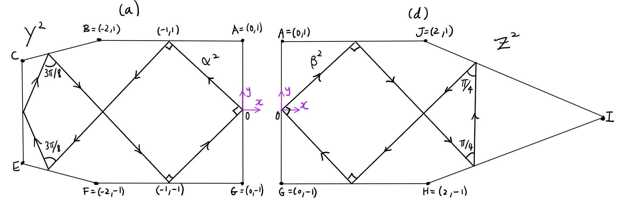
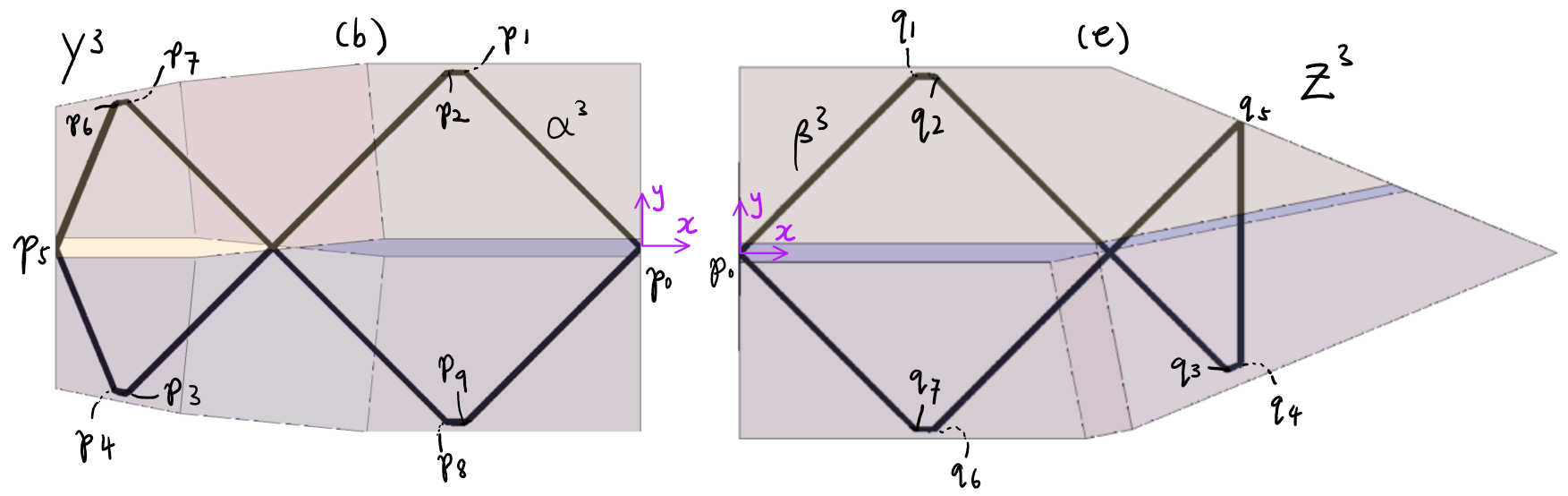
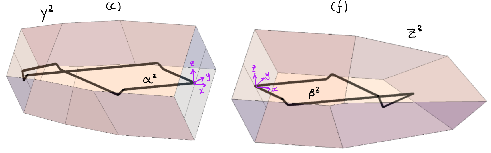
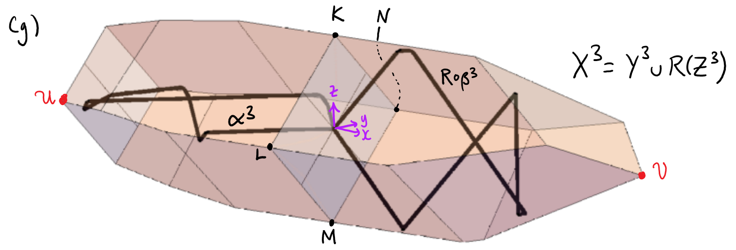
Figure 4.2: Various stages from the construction of a stable figure-eight in the proof of Proposition 4.5, but for a larger value of $\delta$ to make the finer details visible. (a) The polygon $\mathbf{Y}^{2}$ and billiard trajectory $\alpha^{2}$. (b) An origami model $(\mathbf{Y}^{3},\alpha^{3})$ of $(\mathbf{Y}^{2},\alpha^{2})$. $\alpha^{3}$ starts from $p_{0}=(0,0,0)$, collides at $p_{1},\dotsc,p_{9}$, and then returns to $p_{0}$. (c) Another view of $\mathbf{Y}^{3}$ and $\alpha^{3}$. (d) The polygon $\mathbf{Z}^{2}$ and billiard trajectory $\beta^{2}$. (e) An origami model $(\mathbf{Z}^{3},\beta^{3})$ of $(\mathbf{Z}^{2},\beta^{2})$. $\beta^{3}$ starts from $p_{0}$, collides at $q_{1},\dotsc,q_{7}$, and then returns to $p_{0}$. (f) Another view of $\mathbf{Z}^{3}$ and $\beta^{3}$. (g) $\mathbf{X}^{3}$ and the billiard trajectories $\alpha^{3}$ and $R\circ\beta^{3}$ that correspond to the stable figure-eight in Proposition 4.5.

Let $\delta$ be a small positive number. Apply Theorem 3.19 to get an origami model $(\mathbf{Y}^{3},\alpha^{3})$ of $(\mathbf{Y}^{2},\alpha^{2})$, where $\mathbf{Y}^{3}=\operatorname{Bev}(\mathbf{Y}^{2},\{AB,BC,EF,FG\},g)$, $g(AB)=g(EF)=\delta$ and $g(BC)=g(FG)=-\delta$ (“even” in the parity sequence). (Figure 4.2(b)–(c) illustrates $\mathbf{Y}^{3}$ and $\alpha^{3}$ but for $\delta=0.05$, which is large enough for us to see the finer details; $\delta=0.05$ actually produces results that work for our purposes, but technically that is too large to satisfy the hypotheses of Theorem 3.19.) In fact, we will choose $\delta$ small enough to also allow us to apply Theorem 3.19 to get an origami model $(\mathbf{Z}^{3},\beta^{3})$ of $(\mathbf{Z}^{2},\beta^{2})$, where $\mathbf{Z}^{3}=\operatorname{Bev}(\mathbf{Z}^{2},\{GH,HI,JA\},h)$, $h(GH)=-\delta$, $h(HI)=0$ and $h(JA)=\delta$ (“odd” in the parity sequence). Figure 4.2(e)–(f) depicts $\mathbf{Z}^{3}$ and $\beta^{3}$, but again for the too-large value of $\delta=0.05$. As a consequence of the theorem, $\alpha^{3}$ collides at most once with each face of $\mathbf{Y}^{3}$, and similarly for $\beta^{3}$ in $\mathbf{Z}^{3}$.

Next we will prove that we can also choose $\delta$ to be small enough so that $\alpha^{3}$ and $\beta^{3}$ will also be simple. Note that they are already simple in Figure 4.2(g), which uses a larger value of $\delta$, but let us formally justify why that is true for sufficiently small $\delta$. We cannot directly apply Lemma 3.20 because neither $\alpha^{2}$ nor $\beta^{2}$ are simple. On the other hand, the other hypotheses of the lemma are satisfied for sufficiently small $\delta$, and the proof of the lemma only uses the hypothesis that $\alpha^{2}$ is simple to show that two of the horizontal segments of $\alpha^{3}$ can intersect only if they share an endpoint. Yet, two of those horizontal segments could possibly intersect in their interior only if the same is true of their projections under $\operatorname{pr}_{2}$, so they would have to be correspond to $p_{2}p_{3}$ and $p_{7}p_{8}$ in Figure 4.2(b). This would contradict the fact that $\operatorname{height}(p_{2}p_{3})=2\delta$ and $\operatorname{height}(p_{7}p_{8})=-2\delta$. Therefore the rest of the proof of Lemma 3.20 demonstrates that $\alpha^{3}$ is simple, and similarly for $\beta^{3}$. Furthermore, from their construction, it is clear that $\alpha^{3}$ and $\beta^{3}$ intersect only at their common basepoint.

The same value of $\delta$ is used to construct $\mathbf{Y}^{3}$ and $\mathbf{Z}^{3}$ so that the rectangle $KLMN$ (see Figure 4.2(g)) is a face of both $\mathbf{Y}^{3}$ and $\mathbf{Z}^{3}$. Now let $R\in O(3)$ be the reflection that fixes the $x$ coordinate but interchanges the $y$ and $z$ coordinates. Observe that $R$ maps $KLMN$ back to itself, so that $\mathbf{X}^{3}=\mathbf{Y}^{3}\cup R(\mathbf{Z}^{3})$ is a convex polyhedron, and that $R\circ\beta^{3}$ is a billiard trajectory in $\mathbf{X}^{3}$. Figure 4.2(g) illustrates $\mathbf{X}^{3}$, $\alpha^{3}$ and $R\circ\beta^{3}$. This transformation $R$ is applied to ensure that the the tangent vectors of the final billiard trajectories $\alpha^{4}$ and $\beta^{4}$ at the origin will not lie in the same plane, so that the corresponding geodesic loops do not form a closed geodesic. Eventually this will lead to the irreducibility of the final stable figure-eight.

Next, we will construct $\alpha^{4}$ and $\beta^{4}$ from $\alpha^{3}$ and $R\circ\beta^{3}$ using origami models again. Three of the faces of $\mathbf{Y}^{3}$ that $\alpha^{3}$ collides with are inherited from $\mathbf{W}^{h}(CE)$ and $\mathbf{W}^{h}(EF)$; in Figure 4.2(g), they are the three faces around the vertex $u$. Index those faces $A_{1}$, $A_{2}$ and $A_{3}$ in the order that $\alpha^{3}$ collides with them. Similarly, three of the faces that $R\circ\beta^{3}$ collides with are images under $R$ of the faces of $\mathbf{Z}^{3}$ that are inherited from $\mathbf{W}^{h}(HI)$ and $\mathbf{W}^{h}(IJ)$; in Figure 4.2(g), they are the three faces around the vertex $v$. Index those faces $B_{1}$, $B_{2}$ and $B_{3}$ in the order that $\beta^{3}$ collides with them. Apply Theorem 3.19 to get origami models $(\mathbf{X}^{4},\alpha^{4})$ of $(\mathbf{X}^{3},\alpha^{3})$ and $(\mathbf{X}^{4},\beta^{4})$ of $(\mathbf{X}^{3},R\circ\beta^{3})$, where $\mathbf{X}^{4}=\operatorname{Bev}(\mathbf{X}^{3},\mathcal{F},f)$, $\mathcal{F}=\{A_{1},A_{2},A_{3},B_{1},B_{2},B_{3}\}$ and

$$f(A_{1}) =f(B_{1})=\varepsilon$$ (4.3)

$$f(A_{2}) =f(B_{2})=0$$ (4.4)

$$f(A_{3}) =f(B_{3})=-\varepsilon,$$ (4.5)

where $\varepsilon$ is chosen to be sufficiently small to satisfy the hypotheses of Theorem 3.19. (This gives the final “odd” in each parity sequence.)

One can check that $\alpha^{4}$ and $\beta^{4}$ each collide an even number of times, so they correspond to geodesic loops $\gamma_{1}$ and $\gamma_{2}$ in $\mathcal{D}_{\mathrm{}}\mathbf{X}^{4}$ that are based at the same point $p$, giving a stationary figure-eight $G^{4}$. By from [Che22, Corollary 3.4], it remains to prove that $\ker D_{\gamma_{1}}\cap\ker D_{\gamma_{2}}=\{0\}$. Given the parity sequence used to construct $\alpha^{4}$, Lemma 4.2 implies that $\ker D_{\gamma_{1}}=\operatorname{span}\{(0,1,0,0),(0,0,1,0)\}$, under the identification of $T_{p}\mathcal{D}_{\mathrm{}}\mathbf{X}^{4}$ with $\mathbb{R}^{4}$ induced by the quotient map $\mathcal{D}_{\mathrm{}}\mathbf{X}^{4}\to\mathbf{X}^{4}\subset\mathbb{R}^{4}$. A similar application of the arguments used to prove Lemma 4.2 to the parity sequence used to construct $\beta^{4}$, but taking into account the reflection $R$, implies that $\ker D_{\gamma_{2}}=\operatorname{span}\{(1,0,0,0)\}$. Therefore $\ker D_{\gamma_{1}}\cap\ker D_{\gamma_{2}}=\{0\}$.

We could also have chosen $\varepsilon$ small enough to satisfy the hypotheses of Lemma 3.20, to guarantee that $\alpha^{4}$ and $\beta^{4}$ are simple. They also only intersect at their common basepoint, because $\operatorname{im}({\operatorname{pr}_{3}}\circ\alpha^{4})$ lies in the convex hull of $\operatorname{im}(\alpha^{3})$, and similarly for $\beta^{4}$. Thus $G^{4}$ is simple. ∎

Now we will perform the main construction in the proof of the 5-dimensional case of Theorem 1.1.

Proposition 4.6.

There exists a convex 5-polytope $\mathbf{X}^{5}$ and simple billiard loops $\alpha^{5},\beta^{5}$ in $\mathbf{X}^{5}$ that correspond to two geodesic loops of a simple, irreducible and stable figure-eight in $\mathcal{D}_{\mathrm{}}\mathbf{X}^{5}$. Moreover, $\alpha^{5}$ and $\beta^{5}$ intersect only at their common basepoint.

Proof.

We will take the $\mathbf{X}^{3}$, $\alpha^{3}$ and $R\circ\beta^{3}$ from the proof of Proposition 4.5 and “direct sum” with two billiard loops in a convex polygon to get the desired convex 5-polytope $\mathbf{X}^{5}$ and the desired billiard loops $\alpha^{5}$ and $\beta^{5}$, by mimicking the arguments of Section 2. Let us parametrize $\alpha^{3}$ and $R\circ\beta^{3}$ as constant-speed curves over the interval $[0,1]$. Note however that $\alpha^{3}$ and $R\circ\beta^{3}$ each have an odd number of collisions, so they correspond to two geodesics $\phi_{1}$ and $\phi_{2}$ respectively from $(x,0)$ to $(x,1)$, where $(x,0)$ and $(x,1)$ are distinct points in $\mathcal{D}_{\mathrm{}}\mathbf{X}^{3}$—seen as a quotient space of $\mathbf{X}^{3}\times\{0,1\}$—that map to the same point $x$ under the quotient map $q:\mathcal{D}_{\mathrm{}}\mathbf{X}^{3}\to\mathbf{X}^{3}$.

We will also consider a regular decagon $\mathbf{X}^{2}$ and two periodic pentagonal billiard trajectories in it (see Figure 4.3), which we also parametrize as constant-speed curves over $[0,1]$. Due to their odd number of collisions, the pentagonal billiard trajectories also correspond to geodesics $\gamma_{1}$ and $\gamma_{2}$ in $\mathcal{D}_{\mathrm{}}\mathbf{X}^{2}$ from points $(y,0)$ to $(y,1)$ in $\mathcal{D}_{\mathrm{}}\mathbf{X}^{2}$ for some $y\in\mathbf{X}^{2}$. Let $\gamma_{1}$ correspond to the red pentagonal billiard trajectory in Figure 4.3 and let $\gamma_{2}$ correspond to the black one.

Observe that the geodesics $(\phi_{1},\gamma_{1})$ and $(\phi_{2},\gamma_{2})$ in $\mathcal{D}_{\mathrm{}}\mathbf{X}^{3}\times\mathcal{D}_{\mathrm{}}\mathbf{X}^{2}$ project to geodesic loops in $\mathcal{D}_{\mathrm{}}(\mathbf{X}^{3}\times\mathbf{X}^{2})$ under the branched cover $\Gamma:\mathcal{D}_{\mathrm{}}\mathbf{X}^{3}\times\mathcal{D}_{\mathrm{}}\mathbf{X}^{2}\to\mathcal{D}_{\mathrm{}}(\mathbf{X}^{3}\times\mathbf{X}^{2})$ defined in Equation 2.1, as long as each $(\phi_{i},\gamma_{i})$ avoids the branch locus. This is because these geodesic loops will be based at $((x,y),0+0\bmod 2)=((x,y),1+1\bmod 2)$. These two geodesic loops would then form a stationary geodesic bouquet $G$.

As explained in Section 2, $(\phi_{1},\gamma_{1})$ will avoid the branch locus if $\alpha^{3}$ never collides simultaneously with the red pentagonal billiard trajectory. This is true because trigonometry shows that the red trajectory never collides simultaneously with $\alpha^{2}$ from the proof of Proposition 4.5 (parametrized over $[0,1]$), and the collision times of $\alpha^{3}$ can be made arbitrarily close to those of $\alpha^{2}$ by choosing $\delta$ from the proof of Proposition 4.5 to be sufficiently small. A similar argument shows that $R\circ\beta^{3}$ never collides simultaneously with the black pentagonal billiard trajectory. Therefore each $(\phi_{i},\gamma_{i})$ avoids the branch locus, and we have the stationary geodesic bouquet $G$.

We will prove that $G$ is in fact a stable figure-eight. After that, irreducibility can be readily verified. We can also prove that $G$ is simple, because $\alpha^{3}$ and $R\circ\beta^{3}$ are simple loops that intersect only at their common basepoint, and the rest follows from adapting the proof of Lemma 2.3.

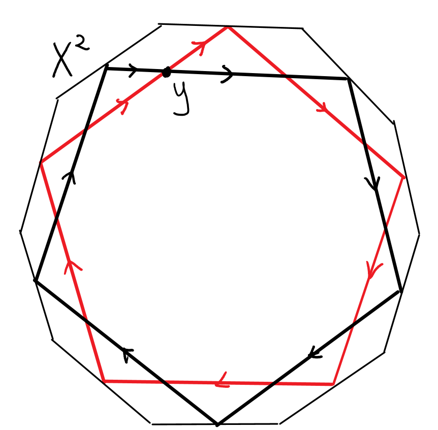
Figure 4.3: A regular decagon $\mathbf{X}^{2}$ with two periodic billiard trajectories, in black and red, starting and ending at a point $y\in\mathbf{X}^{2}$.

We can mimic most of the analysis from Section 2 by defining analogues of the parallel defect operator, studying their kernels, and adapting our notion of stability. We can define the index forms $Q_{\gamma_{i}}$ using the same formulas as in [Che22, Section 3.1]; they are non-negative definite because of the flat metric. We can adapt the proof of Lemma 2.1 to prove the following. Let $W$ be a vector field along $G$ that pulls back along the branched cover $\Gamma$ to a vector field $U+V$ along $(\phi_{1},\gamma_{1})$ and $(\phi_{2},\gamma_{2})$, where $U$ (resp. $V$) is the component in $T\mathcal{D}_{\mathrm{}}\mathbf{X}^{3}$ (resp. $T\mathcal{D}_{\mathrm{}}\mathbf{X}^{2}$). Let $U_{i}$ (resp. $V_{i}$) be the restriction of $U$ (resp. $V$) to $\phi_{i}$ (resp. $\gamma_{i}$) for $i\in\{1,2\}$. Then

$$Q_{G}(W)\geq\Big{(}Q_{\phi_{1}}(U_{1}^{\perp})+Q_{\phi_{2}}(U_{2}^{\perp})\Big{)}+\Big{(}Q_{\gamma_{1}}(V_{1}^{\perp})+Q_{\gamma_{2}}(V_{2}^{\perp})\Big{)},$$ (4.6)

where $U_{i}^{\perp}$ (resp. $V_{i}^{\perp}$) is the component of $U_{i}$ (resp. $V_{i}$) that is orthogonal to $\phi_{i}$ (resp. $\gamma_{i}$).

If $\phi_{1}$ and $\phi_{2}$ formed a stationary geodesic bouquet $F$, and $\gamma_{1}$ and $\gamma_{2}$ formed a stationary geodesic bouquet $F^{\prime}$, the strategy from Section 2 would be to demonstrate that $F$ and $F^{\prime}$ are stable, so that $Q_{G}(W)$ can only vanish if the right-hand side of the above inequality also vanishes, which would imply that $U$ and $V$ are tangent to $F$ and $F^{\prime}$ respectively, which would mean that $W$ is tangent to $G$. (The tangency of a vector field to a stationary geodesic bouquet is defined in [Che22, Section 2.1].) Even though we are not in this situation, we will still be able to show that if the right-hand side of the inequality vanishes, then $U_{i}$ (resp. $V_{i}$) must be tangent to $\phi_{i}$ (resp. $\gamma_{i}$) for $i\in\{1,2\}$. That will complete the proof of this proposition.

First we bound the index forms from below in a manner analogous to [Che22, Proposition 3.3]. In a sense we generalize the theory of parallel defect operators to billiard trajectories. We can define a linear operator $D_{\phi_{1}}:T_{x}\mathbf{X}^{3}\to T_{x}\mathbf{X}^{3}$ by $D_{\phi_{1}}=dR_{F_{k}}\dotsm dR_{F_{1}}\bar{\pi}_{0}-\bar{\pi}_{1}$, where $\alpha^{3}$ collides with the faces $F_{1},\dotsc,F_{k}$, and $\bar{\pi}_{t}$ is projection onto the orthogonal complement of $(\alpha^{3})^{\prime}(t)$. Therefore $\bar{\pi}_{t}$ is related to the projection $\pi_{t}:T_{\phi(t)}\mathcal{D}_{\mathrm{}}\mathbf{X}^{3}\to T_{\phi(t)}\mathcal{D}_{\mathrm{}}\mathbf{X}^{3}$ onto the component orthogonal to $\phi^{\prime}$ via $\bar{\pi}_{t}=dq_{\phi_{1}(t)}\pi_{t}dq_{\phi_{1}(t)}^{-1}$, where $q:\mathcal{D}_{\mathrm{}}\mathbf{X}^{3}\to\mathbf{X}^{3}$ is the canonical quotient map. Observe that $dq_{(x,0)}U_{1}(0)=dq_{(x,1)}U_{1}(1)=u$ for some $u\in T_{x}\mathbf{X}^{3}$, and $dq_{(y,0)}V_{1}(0)=dq_{(y,1)}V_{1}(1)=v$ for some $v\in T_{y}\mathbf{X}^{3}$; it may help to consider the following commutative diagram for all $i=1,2$ and $t\in\{0,1\}$, whose diagonal maps are obtained from the differentials of quotient maps, and where $\Gamma$ is the branched cover defined in Equation 2.1.

(4.7)

If $P:T_{(x,0)}\mathcal{D}_{\mathrm{}}\mathbf{X}^{3}\to T_{(x,1)}\mathcal{D}_{\mathrm{}}\mathbf{X}^{3}$ is the parallel transport map of $\phi_{1}$, then following the proof of [Che22, Proposition 3.3], we have

$$Q_{\phi_{1}}(U_{1}^{\perp}) =\int_{0}^{1}\left\lVert\nabla_{\phi_{1}^{\prime}}U_{1}^{\perp}\right\rVert^{2}\,dt$$ (4.8)

$$\geq\left\lVert P\pi_{0}U_{1}(0)-\pi_{1}U_{1}(1)\right\rVert^{2}$$ (4.9)

$$=\left\lVert P\pi_{0}dq_{(x,0)}^{-1}u-\pi_{1}dq_{(x,1)}^{-1}u\right\rVert^{2}$$ (4.10)

$$=\left\lVert dq_{(x,1)}P\pi_{0}dq_{(x,0)}^{-1}u-dq_{(x,1)}\pi_{1}dq_{(x,1)}^{-1}u\right\rVert^{2}$$ (4.11)

$$(\text{\cite[cite]{[\@@bibref{}{Cheng_StableGeodesicNets}{}{}, Lemma~{}4.2]}}) =\left\lVert dR_{F_{k}}\dotsm dR_{F_{1}}dq_{(x,0)}\pi_{0}dq_{(x,0)}^{-1}u-dq_{(x,1)}\pi_{1}dq_{(x,1)}^{-1}u\right\rVert^{2}$$ (4.12)

$$=\left\lVert dR_{F_{k}}\dotsm dR_{F_{1}}\bar{\pi}_{0}u-\bar{\pi}_{1}u\right\rVert^{2}$$ (4.13)

$$=\left\lVert D_{\phi_{1}}(u)\right\rVert^{2}.$$ (4.14)

Similarly we can define $D_{\phi_{2}}$, $D_{\gamma_{1}}$ and $D_{\gamma_{2}}$ and we have $Q_{\phi_{2}}(U_{2}^{\perp})\geq\left\lVert D_{\phi_{2}}(u)\right\rVert^{2}$ and similar lower bounds for $Q_{\gamma_{1}}$ and $Q_{\gamma_{2}}$.

From now on let us assume that $Q_{G}(W)=0$. Then $u\in\ker D_{\phi_{1}}\cap\ker D_{\phi_{2}}$ and $v\in\ker D_{\gamma_{1}}\cap\ker D_{\gamma_{2}}$. It suffices to show that $\ker D_{\phi_{1}}\cap\ker D_{\phi_{2}}=\{0\}$ and $\ker D_{\gamma_{1}}\cap\ker D_{\gamma_{2}}=\{0\}$, because then we would have $u=0$ and $v=0$. We can then follow the proof of [Che22, Corollary 3.4] to show that since $Q_{\phi_{1}}(U_{1}^{\perp})=0$, $U_{1}^{\perp}$ has to be parallel. But since $u=0$, $U_{1}^{\perp}$ must identically vanish, so $U_{1}$ must be tangent to $\phi_{1}$. The same argument shows that $U_{2}$ must be tangent to $\phi_{2}$ and each $V_{i}$ must be tangent to $\gamma_{i}$.

From the proof of Proposition 4.5, the parallel transport maps of $\alpha^{3}$ and $\beta^{3}$ are $\operatorname{diag}(-1,1,1)$ and $M=\left[\begin{smallmatrix}0&-1&0\\ 1&0&0\\ 0&0&-1\end{smallmatrix}\right]$ respectively. Thus the parallel transport map of $R\circ\beta^{3}$ is $RMR^{-1}=\left[\begin{smallmatrix}0&0&-1\\ 0&-1&0\\ 1&0&0\end{smallmatrix}\right]$. From this it can be computed that $\ker D_{\phi_{1}}$ is the $yz$-plane and $\ker D_{\phi_{2}}$ is the $x$-axis, so they do intersect only at the origin. For the periodic billiard trajectories in $\mathbf{X}^{2}$, the parallel transport map is the reflection that fixes the tangent vector at the basepoint by Lemma 4.1. In fact this implies that $\ker D_{\gamma_{1}}$ and $\ker D_{\gamma_{2}}$ are the lines tangent to the periodic billiard trajectories at the basepoint, which intersect only at the origin. Thus we are done. ∎

Finally we can combine all of our previous results into a proof of our main result, Theorem 1.1.

Proof of Theorem 1.1.

From Propositions 4.3, 4.5 and 4.6 we can derive the convex polytopes $\mathbf{X}^{3}$, $\mathbf{X}^{4}$, and $\mathbf{X}^{5}$ in dimensions 3, 4 and 5 whose doubles contain the stable figure-eights $G^{3}$, $G^{4}$ and $G^{5}$ respectively. For each $n\in\{3,4,5\}$ and $m\geq 0$ we will modify $G^{3}$ into slightly different versions $G^{3}_{1},\dotsc,G^{3}_{m}$ so that together with $G^{n}$ they are all pairwise non-singular. Once we accomplish that, Corollary 2.2 will guarantee that $G^{n}\oplus G^{3}_{1}\oplus\dotsb\oplus G^{3}_{m}$ is a stable figure-eight in the double of a convex polytope in dimension $3m+n$, as explained in Section 2.

We find the $G^{3}_{i}$ by doing the construction in Proposition 4.3 but using different, smaller values of $\delta$. Denote the resulting billiard trajectories by $\alpha^{3}_{\delta}$ and $\beta^{3}_{\delta}$, and the resulting height function on faces of $\mathbf{X}^{2}$ be $h_{\delta}:\mathcal{F}\to\mathbb{R}$. We will show that there exist constants $\mu_{i},\tau_{i}>0$ for $i\in\{1,2,3\}$ such that $\alpha^{3}_{\delta}$ collides at times $\mu_{1}-\tau_{1}\delta$, $\mu_{1}+\tau_{1}\delta$, $\mu_{2}-\tau_{2}\delta$, $\mu_{2}+\tau_{2}\delta$, $\mu_{3}-\tau_{3}\delta$, and $\mu_{3}+\tau_{3}\delta$. The same will be true of $\beta^{3}_{\delta}$. Then clearly there will be an infinite number of ways to choose $\delta$ to obtain all of the necessary $G^{3}_{i}$.

The heights of the horizontal segments of $\alpha^{3}_{\delta}$ and the values of $h_{\delta}(F_{1})$, $h_{\delta}(F_{2})$, and $h_{\delta}(F_{3})$ are all proportional to $\delta$. This implies that for any sufficiently small $\delta,\delta^{\prime}>0$, the part of $\alpha_{\delta}^{3}\cup\partial\mathbf{W}^{h_{\delta}}(F_{i})$ near each $F_{i}\times\mathbb{R}$ is homothetic to the part of $\alpha_{\delta^{\prime}}^{3}\cup\partial\mathbf{W}^{h_{\delta^{\prime}}}(F_{i})$ near $F_{i}\times\mathbb{R}$. This situation is illustrated in Figure 4.4, where we have drawn the unraveled versions of $\alpha_{\delta}^{3}$ and $\alpha_{\delta^{\prime}}^{3}$. We have also drawn how it relates to the unraveled version of $\alpha^{2}$ via the projection $\operatorname{pr}_{2}$. The existence of the constants $\mu_{i}$ and $\tau_{i}$ is then evident.

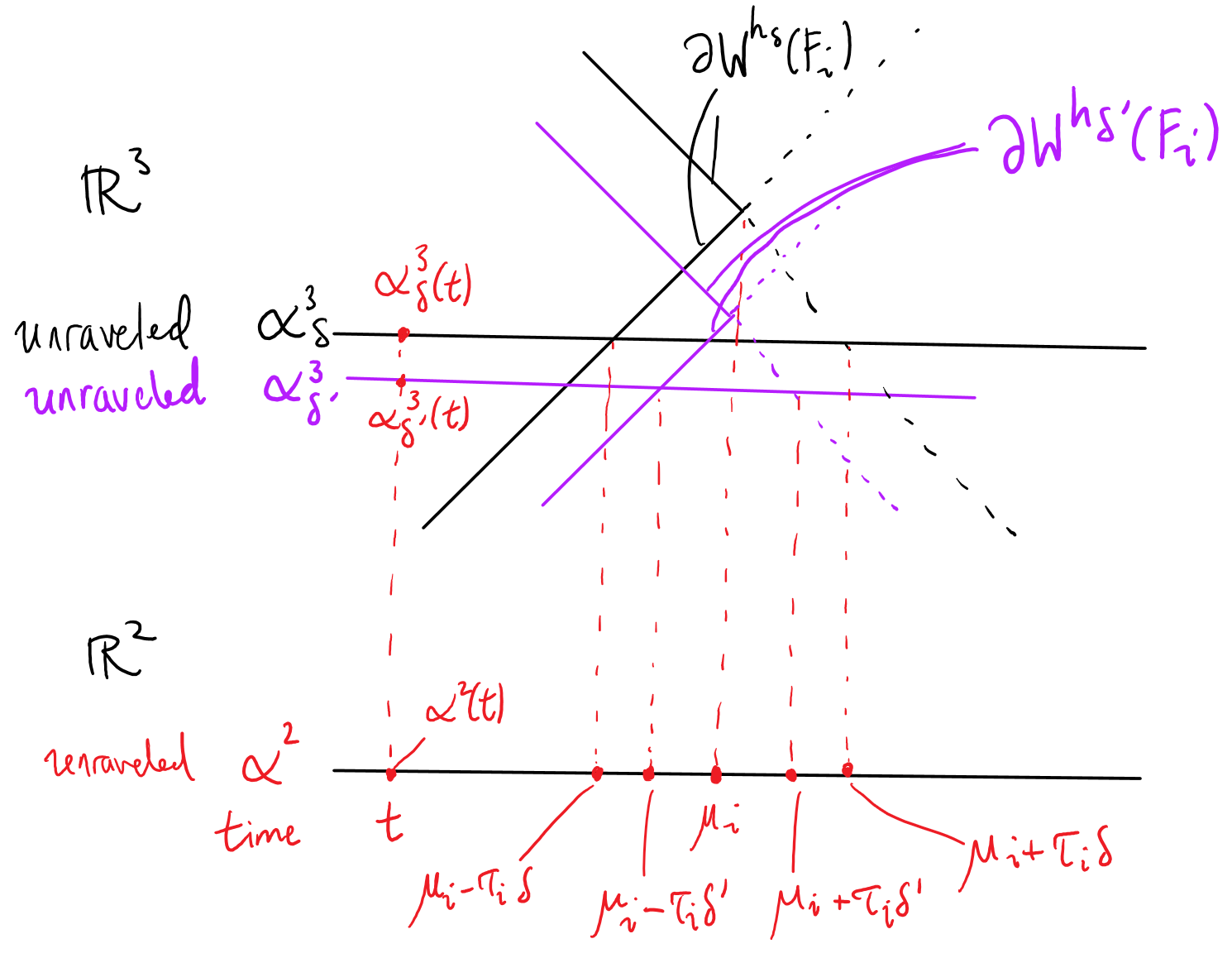
Figure 4.4: Using different values of $\delta$ produces homethetic configurations near collisions.

To complete the proof, it remains to apply [Che22, Propositions 4.7 and 4.8]. ∎

References

- [AA76] William K. Allard and Frederick J. Almgren. The structure of stationary one dimensional varifolds with positive density. Inventiones Mathematicae, 34(2):83–97, 1976.
- [AP20] Ian Adelstein and Franco Vargas Pallete. The length of the shortest closed geodesic on positively curved 2-spheres. arXiv preprint arXiv:2006.04849, pages 1–12, 2020.
- [Che22] Herng Yi Cheng. Stable geodesic nets in convex hypersurfaces, 2022. Submitted to the Journal für die reine und angewandte Mathematik.
- [HM96] Joel Hass and Frank Morgan. Geodesic nets on the 2-sphere. Proceedings of the American Mathematical Society, 124(12):3843–3850, 1996.
- [How85] Ralph Howard. The nonexistence of stable submanifolds, varifolds, and harmonic maps in sufficiently pinched simply connected Riemannian manifolds. Michigan Mathematical Journal, 32(3):321–334, 1985.
- [HW03] Ze-Jun Hu and Guo-Xin Wei. On the nonexistence of stable minimal submanifolds and the Lawson–Simons conjecture. In Colloquium Mathematicum, volume 96, pages 213–223. Instytut Matematyczny Polskiej Akademii Nauk, 2003.
- [Kob58] Shoshichi Kobayashi. Compact homogeneous hypersurfaces. Transactions of the American Mathematical Society, 88(1):137–143, 1958.
- [LJS73] H. Blaine Lawson Jr. and James Simons. On stable currents and their application to global problems in real and complex geometry. Annals of Mathematics, pages 427–450, 1973.
- [LS21] Yevgeny Liokumovich and Bruno Staffa. Generic density of geodesic nets, 2021.
- [NR07] Alexander Nabutovsky and Regina Rotman. Shapes of geodesic nets. Geometry & Topology, 11(2):1225–1254, 2007.
- [Pit74] Jon T. Pitts. Regularity and singularity of one dimensional stationary integral varifolds on manifolds arising from variational methods in the large. In Symposia Mathematica, volume 14, pages 465–472. Academic Press London-New York, 1974.
- [Rot11] Regina Rotman. Flowers on Riemannian manifolds. Mathematische Zeitschrift, 269(1-2):543–554, 2011.
- [SX00] Yi-Bing Shen and Hui-Qun Xu. On the nonexistence of stable minimal submanifolds in positively pinched Riemannian manifolds. In Geometry And Topology Of Submanifolds X, pages 274–283. World Scientific, 2000.
- [Syn36] John Lighton Synge. On the connectivity of spaces of positive curvature. The Quarterly Journal of Mathematics, os-7(1):316–320, 01 1936.
- [Zil76] Wolfgang Ziller. Closed geodesics on homogeneous spaces. Mathematische Zeitschrift, 152(1):67–88, 1976.