Enhancement of incoherent bremsstrahlung in proton-nucleus scattering in the $\Delta$-resonance energy region

Abstract

We investigate emission of the bremsstrahlung photons in the scattering of protons off nuclei at the $\Delta$-resonance energy region. Including properties of $\Delta$-resonance in the nucleus-target to the bremsstrahlung model, we find the following. (1) Ratio between incoherent emission and coherent emission is about $10^{6}$–$10^{7}$ for $p+\isotope[197]{Au}$ (without $\Delta$-resonance) at energy of proton beam $E_{\rm p}$ of 190 MeV, where the calculated full bremsstrahlung spectrum is in good agreement with experimental data. This confirms importance of incoherent processes in study of $\Delta$-resonances in this reaction, which have never been studied yet. We estimate coherent and incoherent contributions, electric and magnetic contributions, full bremsstrahlung spectra for the scattering of protons on the [12]C, [40]Ca, [208]Pb nuclei at $E_{\rm p}=800$ MeV, we find conditions for the most intensive bremsstrahlung emission. (2) Transition $p\,N\to\Delta^{+}N$ in the nucleus-target reinforces emission of bremsstrahlung photons in that reaction at $E_{\rm p}=800$ MeV. Difference between the spectra for normal nuclei and nuclei with included $\Delta$-resonance is larger for more light nuclei, but the spectra are larger for heavier nuclei. (3) Taking into account shortly lived state of $\Delta$-resonance, we find that the spectrum with $\Delta$-resonance in the nucleus-target is essentially larger in the high energy photon region than the spectrum without this $\Delta$-resonance (corresponding calculations for [12][Δ]C, [40][Δ]Ca, [208][Δ]Pb in comparison with [12]C, [40]Ca, [208]Pb are provided). Such an aspect is recommended for registration of $\Delta$-resonances in nuclei in possible future experiments.

I Introduction

Non-nucleon degrees of freedom in nuclei were often studied in nuclear physics Ahrens.1985.NPA ; Gaarde.1991.ARNPS ; Strokovskii.1993.PEPAN . Last years some attention has been focused on hadron excitation of $\Delta(1232)$-resonances in nuclear matter (for brevity, term $\Delta$-resonance in nuclei will be used in this paper) Mukhin.1995.PhysUsp ; Kondratyuk.1994.NPA . Proton, electron, photon and pion can be used as a probe to study such $\Delta$-resonances in nuclei. But, the most easy way to study $\Delta$-resonances in nuclei is based on analysis of scattering of beams of pions on nuclei and photoinduced reactions Nedorezov.2010.book . Last years the proton nucleus scattering has been used as a main reaction for this study, where $\Delta$-resonances are formed in result of virtual pion interaction with one nucleon of nucleus-target Igamkulov.2010.PEPAN . As it was studied in Ref. Gil_Oset.1998.PLB.v416 , coherent photon production in the proton-nucleus scattering is another similar reaction which can be used also for such a study. Interest to emission of photons is explained by that such photons can be measured and new information about physics of formation of $\Delta$-resonance in nuclear matter can be extracted.

However, there is another possibility to study $\Delta$-resonances in nuclei, that is to use analysis of bremsstrahlung photons which are also emitted during such complicated process of proton-nucleus scattering with formation of $\Delta$-resonances. Many effects, like dynamics of the nuclear process, interactions between nucleons, types of nuclear forces, structure of nuclei, quantum effects and anisotropy (deformations), etc. can be included in the model describing the bremsstrahlung emission (for example, see Refs. Maydanyuk.2003.PTP ; Maydanyuk.2006.EPJA ; Maydanyuk.2008.EPJA ; Maydanyuk.2008.MPLA for general properties of bremsstrahlung in $\alpha$ decay, Ref. Maydanyuk.2009.NPA for extraction of information about deformation of nuclei in the $\alpha$ decay from analysis of experimental bremsstrahlung data, Ref. Maydanyuk.2011.JPG for bremsstrahlung in the nuclear radioactivity with emission of protons, Ref. Maydanyuk.2010.PRC for bremsstrahlung in the spontaneous fission of [252]Cf, Ref. Maydanyuk.2011.JPCS for bremsstrahlung in the ternary fission of [252]Cf, Ref. Maydanyuk_Zhang_Zou.2018.PRC for bremsstrahlung in the pion-nucleus scattering from our research, there are many investigations from other researchers). Note perspectives on studying electromagnetic observables of light nuclei based on chiral effective field theory Pastore.2008.PRC (see also research Eden.1996.PRC for $pp$ bremsstrahlung). Experimental measurements of such photons and their analysis provide necessary information about these aspects, model suitability can be therefore verified. So, bremsstrahlung photons is an useful tool to investigate all above questions. This paper is devoted to study $\Delta$-resonances in nuclei by means of bremsstrahlung analysis.

In research  Gil_Oset.1998.PLB.v416 authors provided estimations of cross-sections, where coherent processes were included to the model and calculations. However, analysis of experimental study of bremsstrahlung in proton-nucleus scattering by TAPS collaboration Goethem.2002.PRL indicates that incoherent processes play an important role on the bremsstrahlung emission ($p+\isotope[197]{Au}$ at energy of proton beam of $E_{\rm p}=190$ MeV was studied). There are different reasons to conclude that incoherent emission is more intensive than coherent one. One of them is existence of so called “plateau” in the experimental data in Ref. Goethem.2002.PRL (in the middle part of spectrum). That plateau can be explained if to add incoherent contribution to the formalism. Without this incoherent contribution, the model has only coherent terms and gives spectrum with shape of logarithmic type (i.e., without plateau). In Ref. Maydanyuk_Zhang.2015.PRC ratio between incoherent and coherent contributions was extracted on the basis of analysis of experimental data Goethem.2002.PRL . It was concluded that incoherent bremsstrahlung is intensive (for heavy nuclei used in experiments).

In next research the unified formalism was constructed, which includes both incoherent and coherent contributions. That model allows to estimate ratios for different nuclei and energies of proton beam. From calculations of such ratios we concluded that incoherent contribution is larger essentially for heavy nuclei, than coherent one. Now we found that incoherent and coherent contributions have comparable values for light nuclei (like [4]He, etc.; those processes can be in stars).

After such an research and analysis, there is sense to remind researches Clayton.1992.PRC ; Clayton.1991.PhD . Measurements of bremsstrahlung photons in the proton-nucleus scattering are also presented in those works. Here one can find the spectra with plateou. However, accuracy of data Clayton.1992.PRC ; Clayton.1991.PhD is smaller than data Goethem.2002.PRL . So, before analysis described above, it was unclear about any incoherent emission. So, works Clayton.1992.PRC ; Clayton.1991.PhD could provide the first indications about important role of the incoherent bremsstrahlung in the proton-nucleus processes.

As it was shown in Refs. Maydanyuk_Zhang.2015.PRC , inclusion of relations between spin of the scattered proton and moments of nucleons of nucleus-target to the model allows to essentially improve agreement between theory and experimental data. Without such an inclusion it is impossible to explain presence of plateau in experimental data Goethem.2002.PRL . For the studied reaction incoherent bremsstrahlung contribution is on $10^{6}-10^{7}$ times larger than coherent contribution in the full bremsstrahlung.

As previously a detailed incoherent formalism of emission of bremsstrahlung photons during proton-nucleus scattering was constructed Maydanyuk_Zhang.2015.PRC ; Maydanyuk_Zhang_Zou.2016.PRC ; Liu_Maydanyuk_Zhang_Liu.2019.PRC.hypernuclei , in this paper we apply that model to a new situation where $\Delta$-resonance in nucleus-target can be produced. In particular, we will analyze role of the incoherent processes, and how physics can be changed after its inclusion to analysis.

Photons emitted from incoherent processes have been studied in many topics of nuclear and particle physics. In general, physical picture of the studied reaction becomes more complete, after inclusion of such a type of photons. For example, authors of Ref. Zhu.2015.PRC found not negligible role of incoherent photons in photoproduction of heavy quarks (charm, bottom) and heavy quarkonia [$J/\psi$, $\Upsilon(1S)$] in ultra-peripheral collisions of heavy nuclei Pb–Pb and proton-proton collisions at high energies (see also Refs. Zhu.2016.NPB ; Ma_Zhu.2018.PRD , review Baur.2002.PhysRep ). Incoherent photons have also an important place in study of interactions between dark matter and nuclear matter Bell_Dent.2020.PRD . Generally it is difficult to realize calculations of the spectra including the incoherent contribution. Researchers usually apply different approximations to calculate the coherent processes or incoherent ones Remington.1987.PRC . So, in our research we focus on construction of unified formalism (with corresponding calculations and analysis) with joint description of the coherent and incoherent bremsstrahlung emission. With detailed analysis, we find that the role of incoherent emission is important and the calculated spectra are changed essentially after taking this type of emission into account.

Important parameters in incoherent emission are magnetic moments of nucleons of nucleus and their spins. Spin of $\Delta$-resonance is 3/2, while spins of protons and neutrons of nucleus are 1/2. So, one can suppose that bremsstrahlung emission after inclusion of transition $NN\to\Delta N$ can be changed visibly. This is another motivation of our research in this paper. We would like to check this and to estimate how much is difference will be in emission of photons. Note that investigation in this paper of $\Delta$-resonances in nuclei on the basis of bremsstrahlung analysis (tested on existed experimental data for close processes) is performed at first time.

The paper is organized in the following way. In Sec. II a new model of the bremsstrahlung photons emitted during proton nucleus scattering is presented. In Sec. III we give the results of study for the scattering of protons off the [12]C, [40]Ca, [208]Pb nuclei at proton beam energy of 800 MeV with possible formation of $\Delta$-resonance. We summarize conclusions in Sec. IV. Not published previously details of the model and some useful new calculations are presented in Appendixes A–B.

II Model

II.1 Generalized Pauli equation for nucleons in the proton–nucleus system with $\Delta$-resonance and operator of emission of photons

Let us consider scattering of proton on nucleus in the laboratory frame, where nucleus is consisted on $A-1$ nucleons and one $\Delta$-resonance living short time. We write hamiltonian of such a system with inclusion of emission of photons as many-nucleon generalization of Pauli equation as (obtained from Eq. (1.3.6) in Ref. Ahiezer.1981 , p. 33; this formalism is along Refs. Maydanyuk.2012.PRC ; Maydanyuk_Zhang.2015.PRC ; Maydanyuk_Zhang_Zou.2016.PRC ; Maydanyuk_Zhang_Zou.2018.PRC ; Maydanyuk.2011.JPG , see reference therein)

$$\begin{array}[]{lcl}\vspace{1mm}\hat{H}&=&\biggl{\{}\displaystyle\frac{1}{2m_{p}}\Bigl{(}\hat{\mathbf{p}}_{p}-\displaystyle\frac{z_{p}e}{c}\mathbf{A}_{p}\Bigr{)}^{2}+z_{p}e\,A_{p,0}-\displaystyle\frac{z_{p}e\hbar}{2m_{p}c}\;\mbox{\boldmath$\sigma$}\cdot\mathbf{rot\,A}_{p}\biggr{\}}\;+\par\vspace{1mm}\displaystyle\sum_{j=1}^{A-1}\biggl{\{}\displaystyle\frac{1}{2m_{j}}\Bigl{(}\hat{\mathbf{p}}_{j}-\displaystyle\frac{z_{j}e}{c}\mathbf{A}_{j}\Bigr{)}^{2}+z_{j}e\,A_{j,0}-\displaystyle\frac{z_{j}e\hbar}{2m_{j}c}\;\mbox{\boldmath$\sigma$}\cdot\mathbf{rot\,A}_{j}\biggr{\}}\;+\\ &+&\biggl{\{}\displaystyle\frac{1}{2m_{\Delta}}\Bigl{(}\hat{\mathbf{p}}_{\Delta}-\displaystyle\frac{z_{\Delta}e}{c}\mathbf{A}_{\Delta}\Bigr{)}^{2}+z_{\Delta}e\,A_{\Delta,0}-f_{\Delta}\cdot\displaystyle\frac{z_{\Delta}e\hbar}{2m_{\Delta}c}\;\mbox{\boldmath$\sigma$}\cdot\mathbf{rot\,A}_{\Delta}\biggr{\}}+\par V(\mathbf{r}_{1}\ldots\mathbf{r}_{A-1},\mathbf{r}_{\Delta},\mathbf{r}_{\rm p}).\end{array}$$ (1)

Here, $m_{i}$ and $z_{i}$ are mass and electric charge of nucleon with number $i$, $\hat{\mathbf{p}}_{i}=-i\hbar\,\mathbf{d}/\mathbf{dr}_{i}$ is momentum operator for nucleon with number $i$, $V(\mathbf{r}_{1}\ldots\mathbf{r}_{A-1},\mathbf{r}_{\Delta},\mathbf{r}_{\rm p})$ is a general form of the potential of interactions between nucleons of nucleus, $\Delta$-resonance and the scattered proton, $\sigma$ are Pauli matrixes, $A_{i}=(\mathbf{A}_{i},A_{i,0})$ is a potential of electromagnetic field formed by moving nucleon with number $i$ or $\Delta$-resonance, $A$ in summation is mass number of the nucleus-target. Also we have introduced a new parameter $f_{\Delta}$, related with that Dirac equation is for fermion with spin 1/2, while $\Delta$-resonance has spin 3/2. For $\Delta$-resonance we use analog of Pauli equation with different term of spin (in this paper we assume $f_{\Delta}=3$, as spin of $\Delta$-resonance is 3 times larger than for nucleon).

We rewrite this hamiltonian (1) as

$$\begin{array}[]{lcl}\hat{H}=\hat{H}_{0}+\hat{H}_{\gamma},\end{array}$$ (2)

where

$$\begin{array}[]{lllll}\vspace{1mm}\hat{H}_{0}&=&\displaystyle\frac{1}{2m_{\rm p}}\,\hat{\mathbf{p}}_{\rm p}^{2}+\displaystyle\sum_{j=1}^{A-1}\displaystyle\frac{1}{2m_{j}}\,\hat{\mathbf{p}}_{j}^{2}+\displaystyle\frac{1}{2m_{\Delta}}\,\hat{\mathbf{p}}_{\Delta}^{2}+V(\mathbf{r}_{1}\ldots\mathbf{r}_{A-1},\mathbf{r}_{\Delta},\mathbf{r}_{\rm p}),\\ \vspace{1mm}\hat{H}_{\gamma}&=&\biggl{\{}-\displaystyle\frac{z_{\rm p}e}{m_{\rm p}c}\;\hat{\mathbf{p}}_{\rm p}\cdot\mathbf{A}_{\rm p}+\displaystyle\frac{z_{\rm p}^{2}e^{2}}{2m_{\rm p}c^{2}}\mathbf{A}_{\rm p}^{2}-\displaystyle\frac{z_{\rm p}e\hbar}{2m_{\rm p}c}\,\mbox{\boldmath$\sigma$}\cdot\mathbf{rotA}_{\rm p}+z_{\rm p}e\,A_{\rm p,0}\biggr{\}}\;+\\ &+&\displaystyle\sum_{j=1}^{A-1}\biggl{\{}-\displaystyle\frac{z_{j}e}{m_{j}c}\;\hat{\mathbf{p}}_{j}\cdot\mathbf{A}_{j}+\displaystyle\frac{z_{j}^{2}e^{2}}{2m_{j}c^{2}}\mathbf{A}_{j}^{2}-\displaystyle\frac{z_{j}e\hbar}{2m_{j}c}\,\mbox{\boldmath$\sigma$}\cdot\mathbf{rotA}_{j}+z_{j}e\,A_{j,0}\biggr{\}}\;+\\ &+&\biggl{\{}-\displaystyle\frac{z_{\Delta}e}{m_{\Delta}c}\;\hat{\mathbf{p}}_{\Delta}\cdot\mathbf{A}_{\Delta}+\displaystyle\frac{z_{\Delta}^{2}e^{2}}{2m_{\Delta}c^{2}}\mathbf{A}_{\Delta}^{2}-f_{\Delta}\cdot\displaystyle\frac{z_{\Delta}e\hbar}{2m_{\Delta}c}\,\mbox{\boldmath$\sigma$}\cdot\mathbf{rotA}_{\Delta}+z_{\Delta}e\,A_{\Delta,0}\biggr{\}}.\end{array}$$ (3)

Here, $\hat{H}_{0}$ is hamiltonian describing evolution of nucleons of nucleus and $\Delta$-resonance in the scattering of proton (without emission of photons), $\hat{H}_{\gamma}$ is operator describing emission of bremsstrahlung photons in this scattering.

To include magnetic moments of particles, we change Dirac’s magnetic moment $\mu_{i}^{\rm(Dir)}=z_{i}\,e\hbar/(2m_{i}c)$ for each particle with number $i$ as $\mu_{i}^{\rm(Dir)}\to\mu_{i}^{\rm(an)}\,\mu_{N}$, where $\mu_{N}=e\hbar/(2m_{\rm p}c)$ is nuclear magneton, $\mu_{\rm p}^{\rm(an)}=2.79284734462$ is anomalous magnetic moment for proton, $\mu_{\rm n}^{\rm(an)}=-1.91304273$ is anomalous magnetic moment for neutron $\mu_{j}$ are magnetic moments of protons or neutrons of nucleus (measured in units of nuclear magneton $\mu_{N}$, see Ref. RewPartPhys_PDG.2018 ). We neglect terms at $\mathbf{A}_{j}^{2}$ and $A_{j,0}$, and use Coulomb gauge.

Operator of emission (3) is transformed to

$$\begin{array}[]{llll}\hat{H}_{\gamma}&=&-\displaystyle\frac{z_{\rm p}e}{m_{\rm p}c}\;\hat{\mathbf{p}}_{\rm p}\cdot\mathbf{A}_{\rm p}-\mu_{N}\,\mu_{\rm p}\,\mbox{\boldmath$\sigma$}\cdot\hat{\mathbf{H}}_{\rm p}+\par\displaystyle\sum_{j=1}^{A}\biggl{\{}-\displaystyle\frac{z_{j}e}{m_{j}c}\;\hat{\mathbf{p}}_{j}\cdot\mathbf{A}_{j}-\mu_{N}\,\mu_{j}\,\mbox{\boldmath$\sigma$}\cdot\hat{\mathbf{H}}_{j}\biggr{\}},\end{array}$$ (4)

where

$$\hat{\mathbf{H}}=\mathbf{rot\>A}=\bigl{[}\curl{\mathbf{A}}\bigr{]}$$ (5)

and $\mu_{\Delta}=f_{\Delta}\cdot\mu_{p,\,n}$ ($f_{\Delta}=3$). This expression is many-nucleon generalization of operator of emission $\hat{W}$ in Eq. (4) in Ref. Maydanyuk.2012.PRC with included magnetic moments for nucleons and $\Delta$-resonance.

II.2 Formalism in space representation

Substituting the following definition for the potential of electromagnetic field:

$$\begin{array}[]{lcl}\mathbf{A}&=&\displaystyle\sum\limits_{\alpha=1,2}\sqrt{\displaystyle\frac{2\pi\hbar c^{2}}{w_{\rm ph}}}\;\mathbf{e}^{(\alpha),\,*}e^{-i\,\mathbf{k_{\rm ph}r}},\end{array}$$ (6)

we obtain:

$$\begin{array}[]{lcl}\hat{\mathbf{H}}&=&\bigl{[}\curl{\mathbf{A}}\bigr{]}=\sqrt{\displaystyle\frac{2\pi\hbar c^{2}}{w_{\rm ph}}}\,\displaystyle\sum\limits_{\alpha=1,2}\Bigl{\{}-i\,e^{-i\,\mathbf{k_{\rm ph}r}}\,\bigl{[}\mathbf{k_{\rm ph}}\times\mathbf{e}^{(\alpha),\,*}\bigr{]}+e^{-i\,\mathbf{k_{\rm ph}r}}\,\bigl{[}\curl{\mathbf{e}^{(\alpha),\,*}}\bigr{]}\Bigr{\}}.\end{array}$$ (7)

Here, $\mathbf{e}^{(1)}$ and $\mathbf{e}^{(2)}$ are two independent unit vectors of polarizations for photon [$\mathbf{e}^{(\alpha),*}=\mathbf{e}^{(\alpha)}$, $\alpha=1,2$], $\mathbf{k}_{\rm ph}$ is wave vector of the photon and $w_{\rm ph}=k_{\rm ph}c=\bigl{|}\mathbf{k}_{\rm ph}\bigr{|}c$. Vectors $\mathbf{e}^{(\alpha)}$ are perpendicular to $\mathbf{k}_{\rm ph}$ in Coulomb gauge, satisfy Eq. (8) in Ref. Liu_Maydanyuk_Zhang_Liu.2019.PRC.hypernuclei . One can develop formalism simpler in the system of units where $\hbar=1$ and $c=1$, but we shall write constants $\hbar$ and $c$ explicitly. Also we have properties:

$$\begin{array}[]{lclc}\Bigl{[}\mathbf{k}_{\rm ph}\times\mathbf{e}^{(1)}\Bigr{]}=k_{\rm ph}\,\mathbf{e}^{(2)},&\Bigl{[}\mathbf{k}_{\rm ph}\times\mathbf{e}^{(2)}\Bigr{]}=-\,k_{\rm ph}\,\mathbf{e}^{(1)},&\Bigl{[}\mathbf{k}_{\rm ph}\times\mathbf{e}^{(3)}\Bigr{]}=0,&\displaystyle\sum\limits_{\alpha=1,2,3}\Bigl{[}\mathbf{k}_{\rm ph}\times\mathbf{e}^{(\alpha)}\Bigr{]}=k_{\rm ph}\,(\mathbf{e}^{(2)}-\mathbf{e}^{(1)}).\end{array}$$ (8)

We substitute formulas (6) and (7) to formula (4) for operator of emission and obtain:

$$\begin{array}[]{lcl}\hat{H}_{\gamma}&=&\sqrt{\displaystyle\frac{2\pi\hbar c^{2}}{w_{\rm ph}}}\;\mu_{N}\,\displaystyle\sum\limits_{\alpha=1,2}e^{-i\,\mathbf{k_{\rm ph}r}_{K}}\,\biggl{\{}i\,2z_{\rm p}\,\mathbf{e}^{(\alpha)}\cdot\gradient_{\rm p}+\mu_{\rm p}\,\mbox{\boldmath$\sigma$}\cdot\Bigl{(}i\,\bigl{[}\mathbf{k_{\rm ph}}\times\mathbf{e}^{(\alpha)}\bigr{]}-\bigl{[}\gradient_{\rm p}\times\mathbf{e}^{(\alpha)}\bigr{]}\Bigr{)}\biggr{\}}\;+\\ &+&\sqrt{\displaystyle\frac{2\pi\hbar c^{2}}{w_{\rm ph}}}\;\mu_{N}\,\displaystyle\sum_{j=1}^{A}\displaystyle\sum\limits_{\alpha=1,2}e^{-i\,\mathbf{k_{\rm ph}r}_{j}}\;\biggl{\{}i\,\displaystyle\frac{2z_{j}m_{\rm p}}{m_{Aj}}\>\mathbf{e}^{(\alpha)}\cdot\gradient_{j}+\mu_{j}\,\mbox{\boldmath$\sigma$}\cdot\Bigl{(}i\,\bigl{[}\mathbf{k_{\rm ph}}\times\mathbf{e}^{(\alpha)}\bigr{]}-\bigl{[}\gradient_{j}\times\mathbf{e}^{(\alpha)}\bigr{]}\Bigr{)}\biggr{\}}.\end{array}$$ (9)

This expression coincides with operator of emission $\hat{W}$ in form (6) in Ref. Maydanyuk.2012.PRC in the limit case of problem of one nucleon with charge $Z_{\rm eff}$ in the external field [taking Eqs. (8), $\hbar=1$ into account]. We have included terms for $\Delta$-resonance to summation in Eq. (9) and further in this paper, for convenience.

II.3 Operator of emission with relative coordinates

We define coordinates of center-of-mass for the nucleus as $\mathbf{R}_{A}$, for the complete system as $\mathbf{R}$, relative coordinate $\mathbf{r}$ between the scattered proton and center-of-mass of nucleus-target, relative coordinates $\mbox{\boldmath$\rho$}_{Aj}$ of nucleons (and $\Delta$-resonance) of the nucleus concerning to its center-of-mass. Following to formalism in Ref. Maydanyuk.2012.PRC [see Eqs. (3), (4) and explanation in the text of that paper; also see Appendix A in Ref. Liu_Maydanyuk_Zhang_Liu.2019.PRC.hypernuclei ], we find new relative coordinate $\mathbf{r}=\mathbf{r}_{\rm p}-\mathbf{R}_{A}$, new relative coordinates $\mbox{\boldmath$\rho$}_{Aj}=\mathbf{r}_{Aj}-\mathbf{R}_{A}$ for nucleons for the nucleus. We calculate momentums $\hat{\mathbf{P}}$, $\hat{\mathbf{p}}$, $\mathbf{\tilde{p}}_{Aj}$ corresponding to independent variables $\mathbf{R}$, $\mathbf{r}$, $\mbox{\boldmath$\rho$}_{Aj}$ at $j=1\ldots A-1$ (defined like $\hat{\mathbf{p}}_{i}=-i\hbar\,\mathbf{d}/\mathbf{dr}_{i}$), and rewrite formalism above.

Following to formalism in Ref. Liu_Maydanyuk_Zhang_Liu.2019.PRC.hypernuclei , we calculate operator of emission of bremsstrahlung photons in the scattering of proton off nucleus in the laboratory frame as

$$\hat{H}_{\gamma}=\hat{H}_{P}+\hat{H}_{p}+\Delta\hat{H}_{\gamma E}+\Delta\hat{H}_{\gamma M}+\hat{H}_{k},$$ (11)

where operators $\hat{H}_{P}$, $\hat{H}_{p}$, $\hat{H}_{k}$ are calculated in Eqs. (16)–(19) in Ref. Liu_Maydanyuk_Zhang_Liu.2019.PRC.hypernuclei (at $m_{\alpha}\to m_{p}$ replacement) and (see solutions for $\Delta\hat{H}_{\gamma E}$, $\Delta\hat{H}_{\gamma M}$ in Appendix A in Ref. Maydanyuk_Zhang_Zou.2019.brem_alpha_nucleus.arxiv )

$$\begin{array}[]{lcl}\vspace{0.4mm}\Delta\hat{H}_{\gamma E}&=&-\,\sqrt{\displaystyle\frac{2\pi c^{2}}{\hbar w_{\rm ph}}}\>2\,\mu_{N}\,e^{-i\,\mathbf{k_{\rm ph}}\mathbf{R}}\,\displaystyle\sum\limits_{\alpha=1,2}\mathbf{e}^{(\alpha)}\;\times\\ &\times&\biggl{\{}e^{i\,c_{\rm p}\,\mathbf{k_{\rm ph}}\mathbf{r}}\,\displaystyle\sum_{j=1}^{A-1}\displaystyle\frac{z_{j}\,m_{\rm p}}{m_{Aj}}\,e^{-i\,\mathbf{k_{\rm ph}}\mbox{\boldmath$\rho$}_{Aj}}\,\mathbf{\tilde{p}}_{Aj}-\displaystyle\frac{m_{\rm p}}{m_{A}}\,e^{i\,c_{\rm p}\,\mathbf{k_{\rm ph}}\mathbf{r}}\,\displaystyle\sum_{j=1}^{A}z_{j}\,e^{-i\,\mathbf{k_{\rm ph}}\mbox{\boldmath$\rho$}_{Aj}}\,\displaystyle\sum_{k=1}^{A-1}\mathbf{\tilde{p}}_{Ak}\biggr{\}},\end{array}$$ (12)

$$\begin{array}[]{lll}\vspace{0.4mm}&\Delta\hat{H}_{\gamma M}=-\,i\,\sqrt{\displaystyle\frac{2\pi c^{2}}{\hbar w_{\rm ph}}}\>\mu_{N}\>e^{-i\,\mathbf{k_{\rm ph}}\mathbf{R}}\,\displaystyle\sum\limits_{\alpha=1,2}\;\times\\ \times&\biggl{\{}e^{i\,\mathbf{k_{\rm ph}}c_{\rm p}\,\mathbf{r}}\,\displaystyle\sum_{j=1}^{A-1}\mu_{j}\,e^{-i\,\mathbf{k_{\rm ph}}\mbox{\boldmath$\rho$}_{Aj}}\,\mbox{\boldmath$\sigma$}\cdot\bigl{[}\mathbf{\tilde{p}}_{Aj}\times\mathbf{e}^{(\alpha)}\bigr{]}-\par e^{i\,\mathbf{k_{\rm ph}}c_{\rm p}\,\mathbf{r}}\,\displaystyle\sum_{j=1}^{A}\mu_{j}\,\displaystyle\frac{m_{Aj}}{m_{A}}\,e^{-i\,\mathbf{k_{\rm ph}}\mbox{\boldmath$\rho$}_{Aj}}\,\displaystyle\sum_{k=1}^{A-1}\mbox{\boldmath$\sigma$}\cdot\bigl{[}\mathbf{\tilde{p}}_{Ak}\times\mathbf{e}^{(\alpha)}\bigr{]}\biggr{\}}.\end{array}$$ (13)

Here, new coefficients $c_{A}=\frac{m_{A}}{m_{A}+m_{\rm p}}$ and $c_{\rm p}=\frac{m_{\rm p}}{m_{A}+m_{\rm p}}$ are introduced, where $m_{\rm p}$ and $m_{A}$ are masses of proton scattered and nucleus-target, $m_{Aj}$ is mass of nucleon of nucleus with number $j$, and ($\mathbf{e}^{(\alpha)}$ are perpendicular to $\mathbf{k}_{\rm ph}$ in Coulomb gauge, satisfy Eq. (8) in Ref. Liu_Maydanyuk_Zhang_Liu.2019.PRC.hypernuclei . $A$ in summation is mass number of the nucleus-target.

II.4 Matrix elements of emission of bremsstrahlung photons

We define the wave function of the full nuclear system as $\Psi=\Phi(\mathbf{R})\cdot\Phi_{\rm p-nucl}(\mathbf{r})\cdot\psi_{\rm nucl}(\beta_{A})$ following the formalism in Ref. Maydanyuk_Zhang.2015.PRC for the proton-nucleus scattering [see Sect. II.B, Eqs. (10)–(13)], and we add description of many-nucleon structure of the nucleus as in Ref. Maydanyuk_Zhang_Zou.2016.PRC . Here, $\beta_{A}$ is the set of numbers $1\cdots A$ of nucleons of the nucleus, $\Phi(\mathbf{R})$ is the function describing motion of center-of-mass of the full nuclear system in laboratory frame, $\Phi_{\rm p-nucl}(\mathbf{r})$ is the function describing relative motion of the scattered proton concerning to nucleus (without description of internal relative motions of nucleons in the nucleus), $\psi_{\rm nucl}(\beta_{A})$ is the many-nucleon function of the nucleus, defined in Eq. (12) Ref. Maydanyuk_Zhang.2015.PRC on the basis of one-nucleon functions $\psi_{\lambda_{s}}(s)$, $\beta_{A}$ is the set of numbers $1\cdots A$ of nucleons of the nucleus. One-nucleon functions $\psi_{\lambda_{s}}(s)$ represent the multiplication of space and spin-isospin functions as $\psi_{\lambda_{s}}(s)=\varphi_{n_{s}}(\mathbf{r}_{s})\,\bigl{|}\,\sigma^{(s)}\tau^{(s)}\bigr{\rangle}$, where $\varphi_{n_{s}}$ is the space function of the nucleon with number $s$, $n_{s}$ is the number of state of the space function of the nucleon with number $s$, $\bigl{|}\,\sigma^{(s)}\tau^{(s)}\bigr{\rangle}$ is the spin-isospin function of the nucleon with number $s$.

We define the matrix element of emission, using the wave functions $\Psi_{i}$ and $\Psi_{f}$ of the full nuclear system in states before emission of photons ($i$-state) and after such emission ($f$-state), as

$$F=\langle\Psi_{f}|\,\hat{H}_{\gamma}|\,\Psi_{i}\rangle.$$ (14)

In this matrix element we should integrate over all independent variables i.e. space variables $\mathbf{R}$, $\mathbf{r}$, $\mbox{\boldmath$\rho$}_{Am}$. We should take into account space representation of all used moments $\hat{\mathbf{P}}$, $\hat{\mathbf{p}}$, $\mathbf{\tilde{p}}_{Am}$ (as $\hat{\mathbf{P}}=-i\hbar\,\mathbf{d/dR}$, $\hat{\mathbf{p}}=-i\hbar\,\mathbf{d/dr}$, $\mathbf{\tilde{p}}_{Am}=-i\hbar\,\mathbf{d/d}\mbox{\boldmath$\rho$}_{Am}$). Using formulas (11)–(13) for the operator of emission, we calculate [see Appendix LABEL:sec.app.short.2.7 for details, Eqs. (32), (64)–(LABEL:eq.app.short.2.12.8)]

$$\begin{array}[]{lll}\langle\Psi_{f}|\,\hat{H}_{\gamma}|\,\Psi_{i}\rangle\;\;=\;\;\sqrt{\displaystyle\frac{2\pi\,c^{2}}{\hbar w_{\rm ph}}}\,M_{\rm full},&M_{\rm full}=M_{P}+M_{p}^{(E)}+M_{p}^{(M)}+M_{k}+M_{\Delta E}+M_{\Delta M},\end{array}$$ (15)

where

$$\begin{array}[]{lll}\vspace{-0.2mm}M_{p}^{(E)}&=&2\,i\hbar\,(2\pi)^{3}\displaystyle\frac{m_{\rm p}}{\mu}\>\mu_{N}\displaystyle\sum\limits_{\alpha=1,2}\displaystyle\int\limits\Phi_{\rm p-nucl,f}^{*}(\mathbf{r})\;e^{-i\,\mathbf{k}_{\rm ph}\mathbf{r}}\cdot Z_{\rm eff}(\mathbf{k}_{\rm ph},\mathbf{r})\cdot\mathbf{e}^{(\alpha)}\,\mathbf{\displaystyle\frac{d}{dr}}\cdot\Phi_{\rm p-nucl,i}(\mathbf{r})\;\mathbf{dr},\\ M_{p}^{(M)}&=&-\,\hbar\,(2\pi)^{3}\displaystyle\frac{m_{\rm p}}{\mu}\>\mu_{N}\displaystyle\sum\limits_{\alpha=1,2}\displaystyle\int\limits\Phi_{\rm p-nucl,f}^{*}(\mathbf{r})\;e^{-i\,\mathbf{k}_{\rm ph}\mathbf{r}}\cdot\mathbf{M}_{\rm eff}(\mathbf{k}_{\rm ph},\mathbf{r})\cdot\Bigl{[}\mathbf{\displaystyle\frac{d}{dr}}\times\mathbf{e}^{(\alpha)}\Bigr{]}\cdot\Phi_{\rm p-nucl,i}(\mathbf{r})\;\mathbf{dr},\end{array}$$ (16)

$$\begin{array}[]{lllll}\vspace{-0.1mm}M_{P}&=&\displaystyle\frac{\hbar\,(2\pi)^{3}}{m_{A}+m_{p}}\,\mu_{N}\,\displaystyle\sum\limits_{\alpha=1,2}\displaystyle\int\limits\Phi_{\rm p-nucl,f}^{*}(\mathbf{r})\;\biggl{\{}2\,m_{\rm p}\;\Bigl{[}e^{-i\,c_{A}\,\mathbf{k_{\rm ph}}\mathbf{r}}F_{p,\,{\rm el}}+e^{i\,c_{p}\,\mathbf{k_{\rm ph}}\mathbf{r}}F_{A,\,{\rm el}}\Bigr{]}\,\mathbf{e}^{(\alpha)}\cdot\mathbf{K}_{i}\;+\\ &+&i\>\Bigl{[}e^{-i\,c_{A}\,\mathbf{k_{\rm ph}}\mathbf{r}}\,\mathbf{F}_{p,\,{\rm mag}}+e^{i\,c_{p}\,\mathbf{k_{\rm ph}}\mathbf{r}}\,\mathbf{F}_{A,\,{\rm mag}}\Bigr{]}\cdot\bigl{[}\mathbf{K}_{i}\crossproduct\mathbf{e}^{(\alpha)}\bigr{]}\biggr{\}}\cdot\Phi_{\rm p-nucl,i}(\mathbf{r})\;\mathbf{dr},\end{array}$$ (17)

$$\begin{array}[]{lcl}M_{k}&=&i\,\hbar\,(2\pi)^{3}\mu_{N}\,\displaystyle\sum\limits_{\alpha=1,2}\bigl{[}\mathbf{k_{\rm ph}}\crossproduct\mathbf{e}^{(\alpha)}\bigr{]}\displaystyle\int\limits\Phi_{\rm p-nucl,f}^{*}(\mathbf{r})\cdot\Bigl{\{}e^{-i\,c_{A}\,\mathbf{k_{\rm ph}}\mathbf{r}}\,\mathbf{D}_{p,\,{\rm k}}+e^{i\,c_{p}\,\mathbf{k_{\rm ph}}\mathbf{r}}\,\mathbf{D}_{A,\,{\rm k}}\Bigr{\}}\cdot\Phi_{\rm p-nucl,i}(\mathbf{r})\;\mathbf{dr},\end{array}$$ (18)

$$\begin{array}[]{lll}M_{\Delta E}&=&-\,(2\pi)^{3}\,2\,\mu_{N}\displaystyle\sum\limits_{\alpha=1,2}\mathbf{e}^{(\alpha)}\displaystyle\int\limits\Phi_{\rm p-nucl,f}^{*}(\mathbf{r})\;\biggl{\{}e^{i\,c_{p}\,\mathbf{k_{\rm ph}}\mathbf{r}}\,\mathbf{D}_{A1,\,{\rm el}}-\displaystyle\frac{m_{\rm p}}{m_{A}}\,e^{i\,c_{p}\,\mathbf{k_{\rm ph}}\mathbf{r}}\,\mathbf{D}_{A2,\,{\rm el}}\biggr{\}}\cdot\Phi_{\rm p-nucl,i}(\mathbf{r})\;\mathbf{dr},\end{array}$$ (19)

$$\begin{array}[]{lll}M_{\Delta M}&=&-\,i\,(2\pi)^{3}\,\mu_{N}\,\displaystyle\sum\limits_{\alpha=1,2}\displaystyle\int\limits\Phi_{\rm p-nucl,f}^{*}(\mathbf{r})\;\biggl{\{}e^{i\,c_{p}\,\mathbf{k_{\rm ph}}\mathbf{r}}\;D_{A1,\,{\rm mag}}(\mathbf{e}^{(\alpha)})-e^{i\,c_{p}\,\mathbf{k_{\rm ph}}\mathbf{r}}\;D_{A2,\,{\rm mag}}(\mathbf{e}^{(\alpha)})\biggr{\}}\cdot\Phi_{\rm p-nucl,i}(\mathbf{r})\;\mathbf{dr}\end{array}$$ (20)

and $\mathbf{K}_{i}=\mathbf{K}_{f}+\mathbf{k}_{\rm ph}$. Here, $\mu=m_{\rm p}m_{A}/(m_{\rm p}+m_{A})$ is reduced mass and the effective electric charge and magnetic moment are [see Eqs. (59), (60)]

$$\begin{array}[]{lll}\vspace{1.0mm}Z_{\rm eff}(\mathbf{k}_{\rm ph},\mathbf{r})=e^{i\,\mathbf{k_{\rm ph}}\mathbf{r}}\,\Bigl{[}e^{-i\,c_{A}\mathbf{k_{\rm ph}}\mathbf{r}}\,\displaystyle\frac{m_{A}}{m_{p}+m_{A}}\,F_{p,\,{\rm el}}-e^{i\,c_{p}\mathbf{k_{\rm ph}}\mathbf{r}}\,\displaystyle\frac{m_{p}}{m_{p}+m_{A}}\,F_{A,\,{\rm el}}\Bigr{]},\\ \mathbf{M}_{\rm eff}(\mathbf{k}_{\rm ph},\mathbf{r})=e^{i\,\mathbf{k_{\rm ph}}\mathbf{r}}\,\Bigl{[}e^{-i\,c_{A}\mathbf{k_{\rm ph}}\mathbf{r}}\,\displaystyle\frac{m_{A}}{m_{p}+m_{A}}\,\mathbf{F}_{p,\,{\rm mag}}-e^{i\,c_{p}\mathbf{k_{\rm ph}}\mathbf{r}}\,\displaystyle\frac{m_{p}}{m_{p}+m_{A}}\,\mathbf{F}_{A,\,{\rm mag}}\Bigr{]}.\end{array}$$ (21)

Here, $F_{{\rm p},\,{\rm el}}$, $F_{A,\,{\rm el}}$, $\mathbf{F}_{{\rm p},\,{\rm mag}}$, $\mathbf{F}_{A,\,{\rm mag}}$, $\mathbf{D}_{A1,\,{\rm el}}$, $\mathbf{D}_{A2,\,{\rm el}}$, $D_{A1,\,{\rm mag}}$, $D_{A2,\,{\rm mag}}$, $\mathbf{D}_{{\rm p},\,{\rm k}}$, $\mathbf{D}_{A,\,{\rm k}}$, $D_{{\rm p},P\,{\rm el}}$, $D_{A,P\,{\rm el}}$, $\mathbf{D}_{{\rm p},P\,{\rm mag}}$, $\mathbf{D}_{A,P\,{\rm mag}}$ are electric and magnetic form factors defined in Appendix A.2 [see Eqs. (47), (52), (52), (54), (56)].

II.5 Dipole approximation of effective electric charge and magnetic moment of nuclear system

After calculations, we obtain the matrix elements for the coherent bremsstrahlung [see Appendix B.1, Eqs.(79)]

$$\begin{array}[]{lll}\vspace{1.5mm}M_{p}^{(E,\,{\rm dip})}=i\hbar\,(2\pi)^{3}\displaystyle\frac{2\,\mu_{N}\,m_{\rm p}}{\mu}\;Z_{\rm eff}^{\rm(dip)}\;\displaystyle\sum\limits_{\alpha=1,2}\mathbf{e}^{(\alpha)}\cdot\mathbf{I}_{1},\\ M_{p}^{(M,\,{\rm dip})}=\hbar\,(2\pi)^{3}\,\displaystyle\frac{\mu_{N}}{\mu}\cdot\alpha_{M}\cdot(\mathbf{e}_{\rm x}+\mathbf{e}_{\rm z})\,\displaystyle\sum\limits_{\alpha=1,2}\Bigl{[}\mathbf{I}_{1}\times\mathbf{e}^{(\alpha)}\Bigr{]}\end{array}$$ (22)

and for incoherent bremsstrahlung [Appendixes B.2–B.3, Eqs. (88), (86), (91)]

$$\begin{array}[]{lll}\vspace{1.4mm}M_{\Delta E}=0,\\ \vspace{1.4mm}M_{\Delta M}=i\,\hbar\,(2\pi)^{3}\,\mu_{N}\,f_{1}\cdot|\mathbf{k}_{\rm ph}|\cdot Z_{\rm A}(\mathbf{k}_{\rm ph})\cdot I_{2},\\ M_{k}=-\,i\,\hbar\,(2\pi)^{3}\,\mu_{N}\cdot k_{\rm ph}\,z_{\rm p}\>\mu_{\rm p}\cdot I_{3}-\displaystyle\frac{\bar{\mu}_{\rm pn}}{f_{1}}\cdot M_{\Delta M}.\end{array}$$ (23)

Integrals are

$$\begin{array}[]{lllll}\vspace{0.5mm}\mathbf{I}_{1}=\biggl{\langle}\>\Phi_{\rm p-nucl,f}(\mathbf{r})\;\biggl{|}\,e^{-i\,\mathbf{k}_{\rm ph}\mathbf{r}}\;\mathbf{\displaystyle\frac{d}{dr}}\biggr{|}\>\Phi_{\rm p-nucl,i}(\mathbf{r})\>\biggr{\rangle}_{\mathbf{r}},\\ \vspace{0.5mm}I_{2}=\Bigl{\langle}\Phi_{\rm p-nucl,f}(\mathbf{r})\;\Bigl{|}\,e^{i\,c_{p}\,\mathbf{k_{\rm ph}}\mathbf{r}}\,\Bigr{|}\,\Phi_{\rm p-nucl,i}(\mathbf{r})\>\Bigr{\rangle}_{\mathbf{r}},\\ I_{3}=\Bigl{\langle}\Phi_{\rm p-nucl,f}(\mathbf{r})\;\Bigl{|}\,e^{-i\,c_{A}\,\mathbf{k_{\rm ph}}\mathbf{r}}\,\Bigr{|}\,\Phi_{\rm p-nucl,i}(\mathbf{r})\>\Bigr{\rangle}_{\mathbf{r}}.\end{array}$$ (24)

The effective electric charge and magnetic moment (21) are [see Eqs. (71), (80)]

$$\begin{array}[]{llll}Z_{\rm eff}^{\rm(dip)}(\mathbf{k}_{\rm ph})=\displaystyle\frac{m_{A}\,z_{\rm p}-m_{\rm p}\,Z_{\rm A}(\mathbf{k}_{\rm ph})}{m_{\rm p}+m_{A}},\\ \mathbf{M}_{\rm eff}^{\rm(dip)}(\mathbf{k}_{\rm ph})=\Bigl{[}z_{\rm p}\,m_{A}\,\mu_{\rm p}-Z_{\rm A}(\mathbf{k}_{\rm ph})\>m_{p}\,\bar{\mu}_{\rm pn}\Bigr{]}\cdot\displaystyle\frac{m_{p}}{m_{p}+m_{A}}\;(\mathbf{e}_{\rm x}+\mathbf{e}_{\rm z}),\end{array}$$ (25)

and we obtain

$$\begin{array}[]{lll}\alpha_{M}=\Bigl{[}Z_{\rm A}(\mathbf{k}_{\rm ph})\>m_{p}\,\bar{\mu}_{\rm pn}-z_{\rm p}\,m_{A}\,\mu_{\rm p}\Bigr{]}\cdot\displaystyle\frac{m_{p}}{m_{p}+m_{A}},&f_{1}=\displaystyle\frac{A-1}{2A}\>\bar{\mu}_{\rm pn}.\end{array}$$ (26)

Here, $\bar{\mu}_{\rm pn}=\mu_{\rm p}+\kappa\,\mu_{\rm n}$, $\kappa=(A-N)/N$, $A$ and $N$ are numbers of nucleons and neutrons in nucleus, $\mu_{\rm p}$ and $\mu_{\rm n}$ are magnetic moments of proton and neutron.

Calculation of integrals (24) is straightforward. In result, we obtain:

$$\begin{array}[]{lll}\vspace{1.5mm}M_{p}^{(E,\,{\rm dip})}&\simeq&-\,\hbar\,(2\pi)^{3}\,\displaystyle\frac{2\,\mu_{N}\,m_{\rm p}}{\mu}\;Z_{\rm eff}^{\rm(dip)}\cdot\displaystyle\frac{\sqrt{3}}{6}\cdot J_{1}(0,1,0),\\ \vspace{1.5mm}M_{p}^{(M,\,{\rm dip})}&\simeq&-\,i\,\hbar\,(2\pi)^{3}\,\displaystyle\frac{\mu_{N}\,\alpha_{M}}{\mu}\cdot\displaystyle\frac{\sqrt{3}}{6}\cdot J_{1}(0,1,0),\\ \vspace{1.5mm}M_{\Delta M}&\simeq&\hbar\,(2\pi)^{3}\,\mu_{N}\,f_{1}\,k_{\rm ph}\,Z_{\rm A}(\mathbf{k}_{\rm ph})\cdot\displaystyle\frac{\sqrt{3}}{2}\cdot\tilde{J}\,(-c_{p},0,1,1),\\ M_{k}&\simeq&-\,\hbar\,(2\pi)^{3}\,\mu_{N}\cdot k_{\rm ph}\,z_{\rm p}\>\mu_{\rm p}^{\rm(an)}\cdot\displaystyle\frac{\sqrt{3}}{2}\cdot\tilde{J}\,(c_{A},0,1,1)-\displaystyle\frac{\bar{\mu}_{\rm pn}^{\rm(an)}}{f_{1}}\cdot M_{\Delta M},\end{array}$$ (27)

where

$$\begin{array}[]{llllll}J_{1}(l_{i},l_{f},n)&=&\displaystyle\int\limits^{+\infty}_{0}\displaystyle\frac{dR_{i}(r,l_{i})}{dr}\>R^{*}_{f}(l_{f},r)\,j_{n}(k_{\rm ph}r)\;r^{2}dr,&\tilde{J}\,(c,l_{i},l_{f},n)&=&\displaystyle\int\limits^{+\infty}_{0}R_{i}(l_{i},r)\,R^{*}_{f}(l_{f},r)\,j_{n}(c\,k_{\rm ph}r)\;r^{2}dr.\end{array}$$ (28)

Here, $R_{i,f}$ is radial part of wave function $\Phi_{\rm p-nucl}(\mathbf{r})$ in $i$-state or $f$-state, $j_{n}(k_{\rm ph}r)$ is spherical Bessel function of order $n$.

We define cross-sections of the emitted bremsstrahlung photons on the basis of the full matrix element $p_{fi}$ in frameworks of formalism given in Refs. Maydanyuk_Zhang_Zou.2016.PRC ; Maydanyuk.2012.PRC ; Maydanyuk_Zhang.2015.PRC (see Eq. (22) in Ref. Maydanyuk_Zhang_Zou.2016.PRC , reference therein) and we do not repeat it in this paper. Finally, we obtain the bremsstrahlung cross-sections as

$$\begin{array}[]{llll}\displaystyle\frac{d\sigma}{dw_{\rm ph}}=\displaystyle\frac{e^{2}}{2\pi\,c^{5}}\>\displaystyle\frac{w_{\rm ph}\,E_{i}}{m_{\rm p}^{2}\,k_{i}}\>\bigl{|}p_{fi}\bigr{|}^{2},&\displaystyle\frac{d^{2}\sigma}{dw_{\rm ph}\,d\cos\theta}=\displaystyle\frac{e^{2}}{2\pi\,c^{5}}\>\displaystyle\frac{w_{\rm ph}\,E_{i}}{m_{\rm p}^{2}\,k_{i}}\>\bigl{\{}p_{fi}\displaystyle\frac{d\,p_{fi}^{*}}{d\,\cos\theta}+c.\,c.\bigr{\}},&M_{\rm full}=-\displaystyle\frac{e}{m_{\rm p}}\,p_{fi},\end{array}$$ (29)

where c. c. is complex conjugation. We calculate the different contributions of the emitted photons to the full bremsstrahlung spectrum. For estimation of the interesting contribution, we use the corresponding matrix element of emission. In this paper we calculate the matrix elements on the basis of wave functions with quantum numbers $l_{i}=0$, $l_{f}=1$ and $l_{\rm ph}=1$ [here, $l_{i}$ and $l_{f}$ are orbital quantum numbers of wave function $\Phi_{\rm p-nucl}(\mathbf{r})$ for states before emission of photon and after this emission, $l_{\rm ph}$ is orbital quantum number of photon in the multipole approach].

III Analysis

III.1 The spectra for $\Delta$-nuclei, coherent contributions VS incoherent ones

Previously, processes with emission of photons in the scattering of protons on the [12]C, [40]Ca, [208]Pb nuclei in the $\Delta$-resonance energy region were analyzed Gil_Oset.1998.PLB.v416 . So, we use these nuclei for analysis. To test our calculations of emission of bremsstrahlung photons, we choose the scattering of $p+\isotope[197]{Au}$ at proton beam energy of 190 MeV. Such a choice is explained by the following. We estimate that accuracy of measurements of bremsstrahlung photons and presented data are the highest for the nucleus [197]Au (see Ref. Goethem.2002.PRL ) in comparison with other experiments in measurements of bremsstrahlung in the proton nucleus scattering. Even, if to compare those data with other measurements of bremsstrahlung photons for other nuclear reactions ($\alpha$-decay, fission, $\alpha$-nucleus scattering, nucleus-nucleus scattering), data in Ref. Goethem.2002.PRL were obtained with the highest accuracy (those data provide reach information). So, those data is a good basis for analysis and tests of different models. By such a reason, calculations in this paper are compared with experimental data in Ref. Goethem.2002.PRL for the nucleus [197]Au (at energies of proton beam used in experiments). Those calculations are performed for test the model, before its next use in the paper.

One can note other experimental bremsstrahlung data for $p+\isotope[208]{Pb}$ at energy of proton beam of 140 MeV obtained by Edington and Rose in Ref. Edington.1966.NP , and for $p+\isotope[64]{Cu}$, $p+\isotope[107]{Ag}$ at energy of proton beam of 72 MeV obtained by Kwato Njock et al. in Ref. Kwato_Njock.1988.PLB . One can find some contradiction between those data and data in Ref. Goethem.2002.PRL . But, once again, accuracy of the data in Ref. Goethem.2002.PRL is higher, so we choose data in Ref. Goethem.2002.PRL for tests in the manuscript.

We calculate wave function of relative motion between proton and center-of-mass of nucleus numerically concerning to the proton-nucleus potential in form of $V(r)=v_{c}(r)+v_{N}(r)+v_{\rm so}(r)+v_{l}(r)$, where $v_{c}(r)$, $v_{N}(r)$, $v_{\rm so}(r)$, and $v_{l}(r)$ are Coulomb, nuclear, spin-orbital, and centrifugal components, respectively. Parameters of this potential are defined in Eqs. (46)–(47) in Ref. Maydanyuk_Zhang.2015.PRC . We calculate the bremsstrahlung cross-section by Eq. (29), where we include matrix elements of coherent emission $M_{p}^{(E,\,{\rm dip})}$, $M_{p}^{(M,\,{\rm dip})}$ in Eqs. (22), and matrix elements of incoherent emission $M_{\Delta M}$, $M_{k}$ in Eqs. (23).

Results of previous study of bremsstrahlung emission Maydanyuk_Zhang.2015.PRC ; Maydanyuk.2012.PRC ; Maydanyuk_Zhang_Zou.2016.PRC ; Liu_Maydanyuk_Zhang_Liu.2019.PRC.hypernuclei show that incoherent emission is essentially larger than coherent one. By such a reason, we start calculations for [197]Au, where experimental data exist. Results of such calculations with inclusion of coherent and incoherent contributions in comparison with experimental data are presented in Fig. 1 (a).

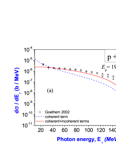
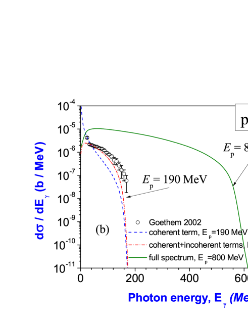
Figure 1: (Color online) Panel (a): The calculated bremsstrahlung spectra (with coherent and incoherent terms) in the scattering of protons off the [197]Au nuclei at energy of proton beam of $E_{\rm p}=190$ MeV in comparison with experimental data Goethem.2002.PRL [matrix elements are defined in Eqs. (22)–(23), $Z_{A}(k_{\rm ph})\simeq Z_{A}$ is electric charge of nucleus, we normalize each calculated spectrum on the second point of experimental data]. Here, experimental data given by open circles (Goethem 2002) are extracted from Ref. Goethem.2002.PRL , blue dashed line is coherent contribution defined by $M_{p}^{(E,\,{\rm dip})}$, red solid line is full spectrum with coherent and incoherent contributions defined by $M_{p}^{(E,\,{\rm dip})}$, $M_{p}^{(M,\,{\rm dip})}$, $M_{\Delta M}$ and $M_{k}$. Panel (b): New calculated spectrum of full bremsstrahlung for [197]Au at energy of proton beam of $E_{\rm p}=800$ MeV in comparison with the bremsstrahlung spectrum for the same reaction at energy of proton beam of $E_{\rm p}=190$ MeV shown in Fig. (a).

The calculated spectra are normalized on one point of these experimental data. This shows that bremsstrahlung model with the coherent and incoherent contributions provides the spectrum in good agreement with experimental data. Note that the first point in experimental data is not explained in satisfactory way by model with included incoherent bremsstrahlung contribution. Without the incoherent contribution, the calculated renormalized spectrum is in worse agreement with experimental data. Presence of such a point could indicate on existence of some unknown processes forming more intensive coherent bremsstrahlung emission at low energies of photons. That problem can motivate on next investigations and developments of the model or more precise measurements of emission of photons at low energies in possible future experiments. But, in current research we omit analysis of this problem.

We obtain

$$\begin{array}[]{lll}M_{p}^{(E,\,{\rm dip})}+M_{p}^{(M,\,{\rm dip})}=M_{p}^{(E,\,{\rm dip})}\cdot\Bigl{\{}1+i\displaystyle\frac{\alpha_{M}}{2\,m_{\rm p}\,Z_{\rm eff}^{\rm(dip)}}\Bigr{\}}.\end{array}$$ (30)

This formula shows role of magnetic emission on the basis of electric one in the full coherent emission of photons. From previous research we know, that increasing of energy of protons beam in nuclear scattering increases intensity of bremsstrahlung emission. Indeed, new calculations for the same scattering $p+\isotope[197]{Au}$ but at energy of protons beam of $E_{\rm p}=800$ MeV are presented in Fig. 1 (b), confirming this property of bremsstrahlung. Also from this figure one can see that difference in intensity of bremsstrahlung for these two cases is essential.

In Fig. 2 we show ratio between contributions of the full incoherent contribution to the full coherent contribution in the bremsstrahlung emission during this scattering process considered above at $E_{\rm p}=190$ MeV.

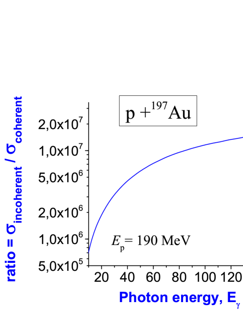
Figure 2: (Color online) Ratio between incoherent and coherent bremsstrahlung contributions in the scattering of protons off the [197]Au nuclei at energy of proton beam of $E_{\rm p}=190$ MeV [matrix elements are defined in Eqs. (22)–(23), $Z_{A}(k_{\rm ph})\simeq Z_{A}$ is electric charge of nucleus ]. In the coherent bremsstrahlung, the magnetic emission based on $M_{p}^{(M,\,{\rm dip})}$ is almost the same as electric emission based on $M_{p}^{(E,\,{\rm dip})}$: we obtain $\frac{\sigma_{\rm mag}^{\rm(coh)}}{\sigma_{\rm el}^{\rm(coh)}}=3.3213$ in the full energy region of photons. In the incoherent bremsstrahlung, role of background emission based on $M_{k}$ is a little larger than magnetic contribution based on $M_{\Delta M}$: we obtain $\frac{\sigma_{\rm background}^{\rm(incoh)}}{\sigma_{\rm mag}^{\rm(incoh)}}=4.04$ in the full energy region of photons.

From this result one can see that role of incoherent emission is essentially larger than coherent emission.

Let us analyze how much the bremsstrahlung spectra are different for different nuclei. Such calculations for the [12]C, [40]Ca, [197]Au, [208]Pb nuclei at energy of proton beam of $E_{\rm p}=800$ MeV are presented in Fig. 3.

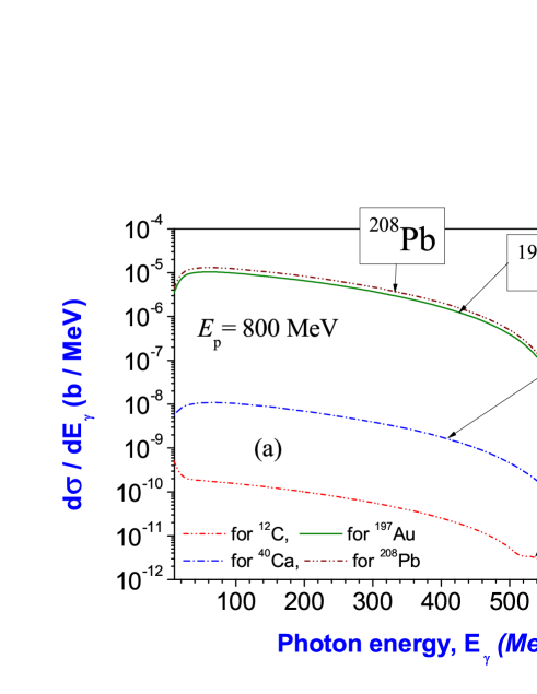
Figure 3: (Color online) The calculated full bremsstrahlung spectra in the scattering of protons off the [12]C, [40]Ca, [197]Au, [208]Pb nuclei at energy of proton beam of $E_{\rm p}=800$ MeV

From this figure one can conclude that probability of emission is larger for heavier nuclei, and difference between the spectra for light and heavy nuclei is essential.

Now let’s suppose possibility of formation of $\Delta$-resonance in the nucleus-target and emission of photons in the scattering, following to Ref. Gil_Oset.1998.PLB.v416 . One can estimate how much the bremsstrahlung emission is changed after inclusion of $\Delta$-resonance to the formalism. For that, one can suppose that such photons are emitted by protons in beam and the modified nucleus, where transition of one nucleon to $\Delta$-resonance takes place (we take transition $pN\to\Delta^{+}N$ in nucleus for analysis in this paper, while another case $nN\to\Delta^{0}N$ can be studied in analogous way).

The first question is in which nuclei are the most convenient to find larger difference between the spectra for normal nuclei and nuclei with included $\Delta$-resonance. Analyzing formalism, one can find that such difference can be from effective electric charge and magnetic moment of proton-nucleus system. Difference between such characteristics is larger for more light nuclei. However, probability of photons for more light nuclei is smaller (see Fig. 3). So, we have unclear situation in finding proper direction. In Fig. 4 we show calculations of the spectra for the [12]C, [40]Ca nuclei in comparison with the [12][Δ]C, [40][Δ]Ca nuclei.

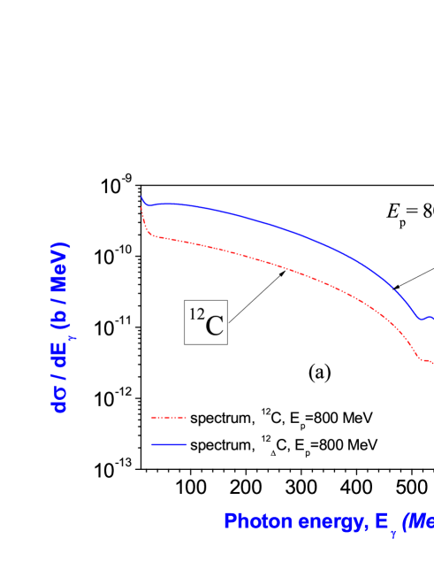
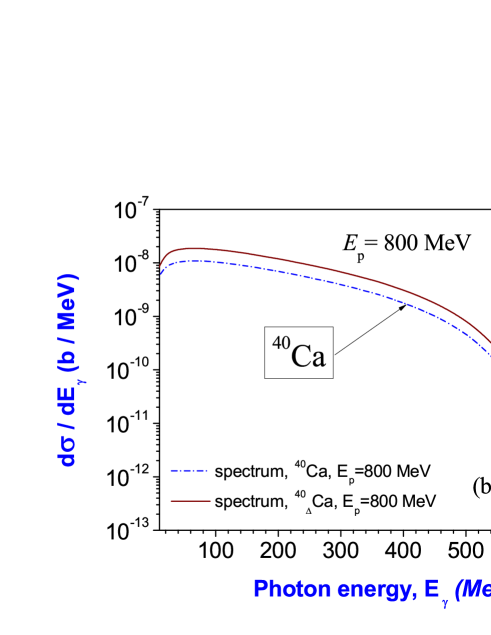
Figure 4: (Color online) The calculated full bremsstrahlung spectra in the scattering of protons off the [12]C, [12][Δ]C nuclei (a) and the [40]Ca, [40][Δ]Ca nuclei (b) at energy of proton beam of $E_{\rm p}=800$ MeV

From such results one can conclude that the bremsstrahlung emission after formation of $\Delta$-resonance from one of nucleons of nucleus is changed not much for light and heavy nuclei, in general.

III.2 Nuclei with highest enhancement of bremsstrahlung due to formation of $\Delta$-resonance

Now we will find nuclei, when transition from nucleon of nucleus to $\Delta$-resonance maximally reinforces the bremsstrahlung emission in the proton nucleus scattering. Parameters important in this task are mass of $\Delta$-resonance, its spin, magnetic moment. Change of mass of baryon in transition from nucleon to $\Delta$-resonances is not much sensitive in calculations of the bremsstrahlung probability, so we will ignore it for more clear understanding of the model. From analysis of the model above we find that the matrix elements $M_{\Delta M}$ and $M_{k}$ defined in Eqs. (23) give the largest contributions to the bremsstrahlung emission. On such a basis, from Eqs. (23) one can find that the most important parameter in this task is $\bar{\mu}_{\rm pn}$. One can see that the highest change of the probability of bremsstrahlung at transition from nucleon to $\Delta$-resonance is in case when $\bar{\mu}_{\rm pn}$ is minimal for normal nucleus. In particular, this is a condition when $\bar{\mu}_{\rm pn}$ is equal to zero for normal nucleus, and we find

$$\begin{array}[]{lll}\displaystyle\frac{Z}{N}=\displaystyle\frac{\mu_{\rm p}}{|\mu_{\rm n}|}=\displaystyle\frac{2.79284734}{1.91304273}=1.459898,\end{array}$$ (31)

where $Z$ and $N$ are numbers of protons and neutrons for the normal nucleus-target. From Eq. (31) one can find more simple condition $Z>N$. Note that unstable nuclei satisfy to this condition mainly which cannot be used as target. However, condition (31) indicates limit, which can be used in analysis to find the proper nucleus from stable isotopes. One can consider Eq. (31) as condition of the highest enhancement of the bremsstrahlung emission due to creation of $\Delta$-resonance in the nucleus-target.

For example, let us look at isotopes of Carbon. Nucleus [12]C does not satisfy to more simple condition as $Z/N=1$. But, unstable nuclear system [10]C satisfies to that condition, and even to condition (31) ($Z/N=1.5$ for [10]C). Results of calculations of the bremsstrahlung spectra for [10]C and [10][Δ]C are shown in Fig. 5.

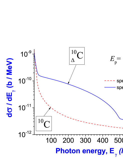
Figure 5: (Color online) The calculated bremsstrahlung spectra in the scattering of protons on [10]C and [10][Δ]C at energy of proton beam of $E_{\rm p}=800$ MeV. One can see that difference between the spectra for [10]C and [10][Δ]C is larger than difference between the spectra for [12]C and [12][Δ]C shown in Fig. 4 (a).

In this figure one can see that the spectrum for [10][Δ]C is larger than the spectrum for [10]C. Comparing with results in Fig. 4 (a), we see that the difference between the spectra for normal nucleus [10]C and $\Delta$-nucleus [10][Δ]C is larger than difference between the spectra for [12]C and [12][Δ]C.

III.3 Bremsstrahlung emission for shortly living $\Delta$-resonance in nucleus

Analyzed maximal enhancement of bremsstrahlung emission presented above is difficult to realize in experiments as condition $Z>N$ is not satisfied for stable nuclei. Moreover, $\Delta$-resonance is shortly living state of baryon (mean lifetime is about $5.58\cdot 10^{-24}$ sec). However, one can remind possibility of emission of bremsstrahlung photons during tunneling in $\alpha$ decay of heavy nuclei analyzed in Refs. Maydanyuk.2006.EPJA ; Maydanyuk.2008.EPJA ; Maydanyuk.2008.MPLA ; Maydanyuk.2009.NPA . As it was shown in Ref. Maydanyuk.2008.MPLA (see Fig. 4 in that paper for [214]Po and [226]Ra), exclusion of possibility of emission of photons from the external space region outside potential barrier of $\alpha$ decay does not decrease the full bremsstrahlung spectrum, but gives opposite effect. In particular, there is destructive interference between bremsstrahlung emission from tunneling region and bremsstrahlung emission from the external region outside barrier. In Fig. 6 (a) we reproduce such an effect for $\alpha$ decay of the [226]Ra nucleus.

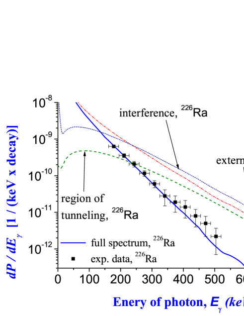
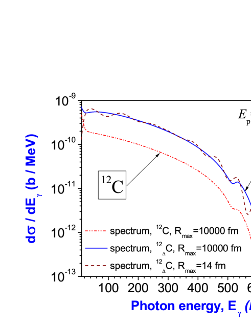
Figure 6: (Color online) Panel (a): The calculated bremsstrahlung contributions in $\alpha$ decay of the [226]Ra nucleus. Panel (b): The calculated bremsstrahlung spectra in the scattering of protons on the [12]C and [12][Δ]C nuclei at energy of proton beam of $E_{\rm p}=800$ MeV at different space region of integration. One can see that the spectrum for at $R_{\rm max}=14$ fm at high energy region (red dashed line) is larger than the spectra at full space region (brown solid line).

In this figure one can see that emission from the tunneling region (see green dashed line in that figure) is larger than the full bremsstrahlung emission (see blue solid line in that figure) at higher energies of photon. But the full bremsstrahlung emission is in good agreement with experimental data that confirms existence of such an effect of destructive interference. This picture is general for bremsstrahlung in the $\alpha$ decay of different nuclei.

This property can be used in our current research of study of $\Delta$-resonance in nuclei. $\Delta$-resonance is shortly lived baryon, so it is formed in nucleus-target only during propagation of the scattered proton (from beam) through the space region of this nucleus. So, we will take into account only this space region of proton-nucleus system in calculation of matrix elements of emission and we will estimate the bremsstrahlung spectra. Energy of proton in beam is much larger than barrier of the proton nucleus potential. However, in calculation of the bremsstrahlung matrix elements we use two wave functions of proton-nucleus scattering — these are wave functions in states before and after emission of photon. In particular, after emission of photon, energy of relative motion of proton concerning to nucleus is reduced on the energy of the photon emitted. So, at enough high energies of the emitted photons wave function in the final state reaches under-barrier energies with tunneling through the barrier. So, in high energy region of photons we have also phenomenon of destructive interference between contributions of emission from the tunneling region and from the external region outside barrier. In particular, on the basis of this logic one can suppose that the spectrum for the shorty lived $\Delta$-resonance in nucleus-target should be larger in the high energy photon region than spectrum of the full emission in the previous figures. Results of such calculations of the spectrum for [12][Δ]C in comparison with previous results are shown in Fig. 6 (b). In next Fig. 7 we present similar calculations of the spectra for the [40][Δ]Ca and [208][Δ]Pb nuclei.

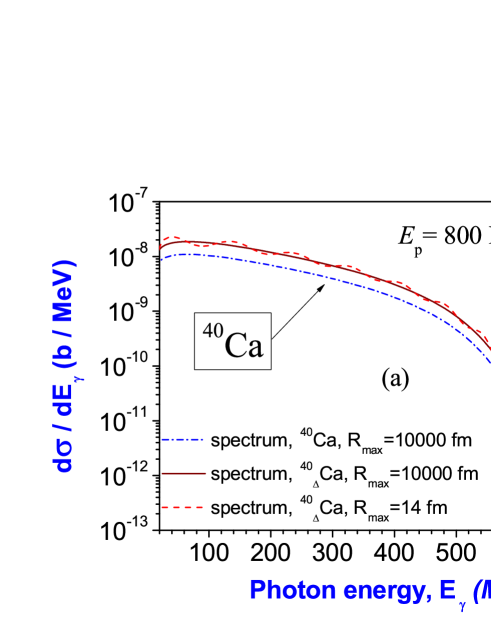
Figure 7: (Color online) The calculated bremsstrahlung spectra in the scattering of protons on the [40]Ca and [40][Δ]Ca nuclei (a) and the [208]Pb and [208][Δ]Pb nuclei (b) at energy of proton beam of $E_{\rm p}=800$ MeV at different space regions of integration. One can see that the spectrum for at $R_{\rm max}=14$ fm at high energy region is larger than the spectra at full space region.

Calculations in these figures confirm our logic above.

III.4 Correction of the spectra on the basis of difference in masses for nucleon and $\Delta$-resonance

The $\Delta$-resonance is nearly 300 MeV heavier than the nucleon. This mass difference is of the same order of magnitude as the photon and incoming-proton energies under study. One can analyze if to neglect this difference in masses is a good approximation.

Reduced mass of proton-nucleus system is a main parameter, which is changed after inclusion of such a correction (difference between masses for proton and $\Delta$-resonance). From previous study we conclude that relative motion of proton (in beam) and nucleus is the most important process forming the largest emission of photons. Here, reduced mass is important parameter (it is used in calculations of wave functions of relative motion for states before and after emission of photons, also in formulas for operator of emission of photons). One can consider two following cases.

• One of protons of nucleus is changed to $\Delta$ resonance. We obtain new reduced mass as $\mu^{\rm(cor,\,1)}=m_{p}\,m_{A}^{\rm(cor)}/(m_{\rm p}+m_{A}^{\rm(cor)})$, where $m_{A}^{\rm(cor)}=m_{\Delta}+(Z-1)m_{p}+(A-Z)\,m_{\rm n}$.

• Proton from beam is changed to $\Delta$ resonance. We obtain new reduced mass as $\mu^{\rm(cor,\,2)}=m_{\Delta}m_{A}/(m_{\Delta}+m_{A})$.

Here, $m_{\rm p}$, $m_{\rm n}$, $m_{\Delta}$ are masses of proton, neutron and $\Delta$-resonance, $m_{A}$ is mass of nucleus, $Z$ and $A$ are numbers of protons and nucleons in nucleus. Calculations of the bremsstrahlung spectra on the basis of these two corrected reduced masses are presented in the new Fig. 8 (a) for [12][Δ]Ca [for comparison, two old spectra from Fig. 4 (a) are used also].

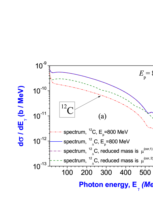
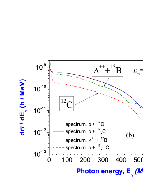
Figure 8: (Color online) The calculated full bremsstrahlung spectra in the scattering of protons off the [12]C, [12][Δ^+]C, [12][Δ^++]C nuclei (a) and in the scattering $\Delta^{++}+\isotope[12]{B}$ (b) at energy of beam of $E=800$ MeV. [Panel (a)]: Corrections of the spectra on the basis of taking into account difference between masses of $\Delta$-resonance and nucleon in calculations. [Panel (b)]: The new spectra at transition $pp\to\Delta^{++}n$ in the nuclear system (see text for explanation).

The spectrum for the first case almost coincides with old spectrum for [12][Δ]Ca [see the purple dash-dotted line in Fig. 8 (a)] (difference between two spectra is in 2-nd or 3-d digits). But, the spectrum for the second case is visibly different from the previous spectrum for [12][Δ]Ca [see the green dashed line in Fig. 8 (a)]. Difference between old spectra [in Fig. 4 (a)] is larger.

Another transition $pN\to\Delta+N$ is also possible in this problem, when the final nucleon can be different from the initial one (e.g. $pp\to\Delta^{++}n$). To analyze this transition, one can consider two following processes.

• Two protons of nucleus are changed to $\Delta^{++}$ resonance and neutron in this nucleus.

• Proton from beam is changed to $\Delta^{++}$ resonance, and one neutron of nucleus is changed to proton.

One could suppose that the second case gives essential changes of the bremsstrahlung spectrum. Interesting analysis can be obtained from such modifications of that reaction under study. Electric charge of the scattered fragment is increased almost twice! In result, effective electric charge $Z_{\rm eff}$ of the nuclear system is increased almost 4 times in dependence on the nucleus-target (i.e., $Z_{\rm eff}^{\rm(new)}=1.304065$ and $Z_{\rm eff}^{\rm(old)}=0.3039928$ for $p+\isotope[12]{C}$). This effective charge is included to the matrix element of coherent bremsstrahlung emission [see Eqs. (24)–(28)]. So, this contribution is increased almost 4 times. However, incoherent bremsstrahlung contribution is larger than coherent one. And this incoherent term does not include effective charge. So, summarized full spectrum is not deformed much. This situation is shown by new green dash-dotted line in new Fig. 8 (b). By simple words, one can suppose that magnetic field of nuclear system is more important that electric field in emission of photons.

The first process is calculated for $p+\isotope[12][\Delta^{++}]{C}$ at energy of beam $E_{\rm p}=800$ MeV and shown in Fig. 8 (b) by new brown dashed line. One can see that this spectrum is very close to blue solid line in this figure.

Also we add calculations of the bremsstrahlung spectra in dependence on mass of nucleus-target (where $\Delta$-resonance is included). Such calculations are presented in Fig. 9.

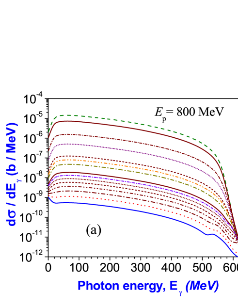
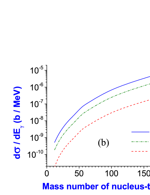
Figure 9: (Color online) The calculated full bremsstrahlung spectra in dependence on mass of nucleus-target (with included $\Delta$-resonance) in the scattering of protons at energy of proton beam of $E_{\rm p}=800$ MeV

One can see that the cross-section of bremsstrahlung emission is increased monotonously at increasing of mass of nucleus-target. Note that wave function of relative motion (for states before emission of photons and after such emission) is calculated on the basis of proton-nucleus potential, which is determined concerning to numbers of protons and neutrons in nucleus-target, according to Ref. Becchetti.1969.PR (that potential is also extrapolated for region of light nuclei). Dependence of the bremsstrahlung spectra on the numbers of protons and neutrons in the nucleus-target can be explained by the following reasons: (1) Calculations of proton-nucleus wave functions on the basis of such a potential, (2) Dependence of operator of emission of photon on the numbers of protons and neutrons in the nucleus-target.

IV Conclusions and perspective

In this paper we investigate emission of the bremsstrahlung photons in the scattering of protons off nuclei at the $\Delta$-resonance energy region. A special focus in this research is directed on question of how much the bremsstrahlung spectrum is changed after transition of one nucleon in nucleus to $\Delta$-resonance. For this research, we improve our previous bremsstrahlung formalism (see Ref. Maydanyuk_Zhang_Zou.2019.PRC.microscopy , reference therein), including new aspects for $\Delta$-resonance in nucleus-target. On such a basis we estimate the spectra of the bremsstrahlung photons and find the following.

• For start of analysis, we calculate the bremsstrahlung spectra in the scattering of protons on the [12]C, [40]Ca, [208]Pb nuclei at energy of proton beam $E_{\rm p}$ of 800 MeV (see Fig. 3). In these calculations we include coherent and incoherent bremsstrahlung contributions, we test this formalism and calculations for the [197]Au nucleus at $E_{\rm p}=190$ MeV on the experimental data Goethem.2002.PRL (see Fig. 1 (a)). We estimate that incoherent emission is essentially more intensive than coherent one (see Fig. 2, ratio between such contributions is about $10^{6}$–$10^{7}$ for $p+\isotope[197]{Au}$ at $E_{\rm p}=190$ MeV, this result is in agreement with results in Refs. Maydanyuk_Zhang.2015.PRC ; Maydanyuk_Zhang_Zou.2016.PRC ; Liu_Maydanyuk_Zhang_Liu.2019.PRC.hypernuclei ). This incoherent contribution is directly dependent on magnetic moments of nucleons of nucleus-target [see Eqs. (22), (23), (26)]. This confirms our supposition that inclusion of incoherent processes in study of $\Delta$-resonance in proton-nucleus scattering is important (as can change picture of the studied process). This aspect has never been studied before, so it is one of aims of this paper.

• We show that increasing of energy of protons beam in nuclear scattering increases intensity of bremsstrahlung emission [see Fig. 1 (b) for comparison, test with experimental data]. Bremsstrahlung emission is larger for heavier nuclei, difference between the spectra for light and heavy nuclei is essential (see Fig. 3 for [12]C, [40]Ca, [197]Au, [208]Pb, difference is about $10^{5}$ times between the spectra for [208]Pb and [12]C at $E_{\rm p}=800$ MeV).

• We analyze coherent and incoherent contributions, electric and magnetic contributions in the full bremsstrahlung for different nuclei and energies of proton beam [see Eqs. (22)–(23)]. In the coherent bremsstrahlung, the magnetic emission is almost the same as electric emission [$\sigma_{\rm mag}^{\rm(coh)}/\sigma_{\rm el}^{\rm(coh)}=3.3213$ for [197]Au at $E_{\rm p}=190$ MeV for 10–180 MeV of photons; see Eq. (30)]. In the incoherent bremsstrahlung, role of background emission based on $M_{k}$ is a little larger than magnetic contribution based on $M_{\Delta M}$ ($\sigma_{\rm background}^{\rm(incoh)}/\sigma_{\rm mag}^{\rm(incoh)}=4.04$ for [197]Au at $E_{\rm p}=190$ MeV for 10–180 MeV of photons). Ratio between incoherent emission and coherent emission is increased at increasing of energy of photon emitted (see Fig. 2, for [197]Au at $E_{\rm p}=190$ MeV).

• For inclusion of transition from proton of nucleus-target to $\Delta^{+}$-resonance ($p\,N\to\Delta^{+}N$) in the proton-nucleus scattering to the model, we use scheme of the coherent processes described in Ref. Gil_Oset.1998.PLB.v416 . We find that emission of bremsstrahlung photons in that reaction with one $\Delta$-resonance in nucleus-target is more intensive than for normal nucleus (see Fig. 4 for [12]C, [12][Δ]C and [40]Ca, [40][Δ]Ca at $E_{\rm p}=800$ MeV). This result is indication of reinforcement of bremsstrahlung in proton-nucleus scattering. We find that difference between the spectra for normal nuclei and nuclei with included $\Delta$-resonance is larger for more light nuclei, but the spectra are larger for heavier nuclei (see Fig. 4 for [12]C, [40]Ca in comparison with [12][Δ]C, [40][Δ]Ca).

• In order to find nuclei with maximal reinforcement of bremsstrahlung due to transition $p\,N\to\Delta^{+}N$, we performed analysis and obtained condition (23) determining ratio between protons and neutrons for the normal nucleus. On the example for [10][Δ^+]C, we show that difference between the spectra for [10]C and [10][Δ^+]C is larger essentially than difference between the spectra for [12]C and [12][Δ^+]C (see Fig. 5). However, stable nuclei (like [12]C, [40]Ca, [208]Pb) do not satisfy to that condition (23). As parameter $\bar{\mu}_{\rm pn}$ has the highest influence on reinforcement of bremsstrahlung of such a type, it confirms importance of incoherent processes in this research (i.e., there is no enhancement of bremsstrahlung due to transition $p\,N\to\Delta^{+}N$, if incoherent processes are not included to the model).

• We take into account that $\Delta$-resonance is shortly lived baryon, and it is formed in nucleus-target only during propagation of the scattered proton (from beam) through the space region of this nucleus. On such a basis, we calculate new bremsstrahlung spectra and find that the spectrum for the shorty lived $\Delta$-resonance in the nucleus-target should be larger in the high energy photon region than the spectrum without creation of $\Delta$-resonance in nucleus-target (see Figs. 6 (b), 7 for [12][Δ]C, [40][Δ]Ca, [208][Δ]Pb). This effect has the same origin as phenomenon of destructive interference between emission from tunneling region and external region investigated for bremsstrahlung in the $\alpha$ decay (see Fig. 6 (a) for [226]Ra, also Ref. Maydanyuk.2008.MPLA ).

If to compare the spectra for normal nuclei with the spectra for nuclei with the shortly lived $\Delta$-resonance, then one can see essential difference between these spectra at high energy region of photons. This property can be used for proposal for future experiments with measurements of photons, as tools to distinguish process of formation of $\Delta$-resonance in the nucleus-target.

Appendix A Matrix element of emission

In this Appendix we calculate the matrix element of emission. Substituting formulas (11)–(13) for operator of emission to (14), we obtain:

$$\langle\Psi_{f}|\,\hat{H}_{\gamma}|\,\Psi_{i}\rangle\;\;=\;\;\sqrt{\displaystyle\frac{2\pi\,c^{2}}{\hbar w_{\rm ph}}}\,\Bigl{\{}M_{P}+M_{p}+M_{k}+M_{\Delta E}+M_{\Delta M}\Bigr{\}},$$ (32)

where

$$\begin{array}[]{lcl}\vspace{1mm}M_{P}&=&\sqrt{\displaystyle\frac{\hbar w_{\rm ph}}{2\pi c^{2}}}\;\matrixelement{\Psi_{f}\,}{\hat{H}_{P}}{\,\Psi_{i}}\;=\\ &=&-\,\displaystyle\frac{1}{m_{A}+m_{\rm p}}\,\displaystyle\sum\limits_{\alpha=1,2}\biggl{\langle}\Psi_{f}\,\biggl{|}\,2\,\mu_{N}\,m_{\rm p}\;e^{-i\,\mathbf{k_{\rm ph}}\mathbf{R}}\biggl{\{}z_{\rm p}\,e^{-i\,c_{A}\,\mathbf{k_{\rm ph}}\mathbf{r}}+e^{i\,c_{\rm p}\,\mathbf{k_{\rm ph}}\mathbf{r}}\displaystyle\sum_{j=1}^{A}z_{j}\,e^{-i\,\mathbf{k_{\rm ph}}\mbox{\boldmath$\rho$}_{Aj}}\biggr{\}}\,\mathbf{e}^{(\alpha)}\cdot\hat{\mathbf{P}}+\\ &+&i\>\mu_{N}\,e^{-i\,\mathbf{k_{\rm ph}}\mathbf{R}}\,\biggl{\{}e^{-i\,c_{A}\,\mathbf{k_{\rm ph}}\mathbf{r}}\,\mu_{\rm p}\,m_{\rm p}\,\mbox{\boldmath$\sigma$}+e^{i\,c_{\rm p}\,\mathbf{k_{\rm ph}}\mathbf{r}}\,\displaystyle\sum_{j=1}^{A}\mu_{j}\,m_{Aj}\,e^{-i\,\mathbf{k_{\rm ph}}\mbox{\boldmath$\rho$}_{Aj}}\,\mbox{\boldmath$\sigma$}\biggr{\}}\,\cdot\bigl{[}\hat{\mathbf{P}}\crossproduct\mathbf{e}^{(\alpha)}\bigr{]}\,\biggr{|}\,\Psi_{i}\biggr{\rangle},\end{array}$$ (33)

$$\begin{array}[]{lcl}\vspace{1mm}M_{p}&=&\sqrt{\displaystyle\frac{\hbar w_{\rm ph}}{2\pi c^{2}}}\;\matrixelement{\Psi_{f}\,}{\hat{H}_{p}}{\,\Psi_{i}}\;=\\ &=&-\displaystyle\sum\limits_{\alpha=1,2}\biggl{\langle}\Psi_{f}\,\biggl{|}\,2\,\mu_{N}\,m_{\rm p}\,e^{-i\,\mathbf{k_{\rm ph}}\mathbf{R}}\biggl{\{}e^{-i\,c_{A}\mathbf{k_{\rm ph}}\mathbf{r}}\,\displaystyle\frac{z_{\rm p}}{m_{\rm p}}-e^{i\,c_{\rm p}\mathbf{k_{\rm ph}}\mathbf{r}}\,\displaystyle\frac{1}{m_{A}}\,\displaystyle\sum_{j=1}^{A}z_{j}\,e^{-i\,\mathbf{k_{\rm ph}}\mbox{\boldmath$\rho$}_{Aj}}\biggr{\}}\;\mathbf{e}^{(\alpha)}\cdot\hat{\mathbf{p}}\;+\\ &+&i\,\mu_{N}\,e^{-i\,\mathbf{k_{\rm ph}}\mathbf{R}}\biggl{\{}e^{-i\,c_{A}\mathbf{k_{\rm ph}}\mathbf{r}}\displaystyle\frac{1}{m_{\rm p}}\,\mu_{\rm p}\,m_{\rm p}\,\mbox{\boldmath$\sigma$}-e^{i\,c_{\rm p}\mathbf{k_{\rm ph}}\mathbf{r}}\displaystyle\frac{1}{m_{A}}\displaystyle\sum_{j=1}^{A}\mu_{j}\,m_{Aj}\;e^{-i\,\mathbf{k_{\rm ph}}\mbox{\boldmath$\rho$}_{Aj}}\,\mbox{\boldmath$\sigma$}\biggr{\}}\cdot\bigl{[}\hat{\mathbf{p}}\times\mathbf{e}^{(\alpha)}\bigr{]}\biggr{|}\,\Psi_{i}\,\biggr{\rangle},\end{array}$$ (34)

$$\begin{array}[]{lcl}\vspace{1mm}M_{k}&=&\sqrt{\displaystyle\frac{\hbar w_{\rm ph}}{2\pi c^{2}}}\;\matrixelement{\Psi_{f}\,}{\hat{H}_{k}}{\,\Psi_{i}}\;=\\ &=&i\,\hbar\,\mu_{N}\,\displaystyle\sum\limits_{\alpha=1,2}\biggl{\langle}\Psi_{f}\,\biggl{|}\,e^{-i\,\mathbf{k_{\rm ph}}\mathbf{R}}\biggl{\{}e^{-i\,c_{A}\,\mathbf{k_{\rm ph}}\mathbf{r}}\,\mu_{\rm p}\,\mbox{\boldmath$\sigma$}+e^{i\,c_{\rm p}\,\mathbf{k_{\rm ph}}\mathbf{r}}\,\displaystyle\sum_{j=1}^{A}\mu_{j}\,e^{-i\,\mathbf{k_{\rm ph}}\mbox{\boldmath$\rho$}_{Aj}}\,\mbox{\boldmath$\sigma$}\biggr{\}}\cdot\bigl{[}\mathbf{k_{\rm ph}}\crossproduct\mathbf{e}^{(\alpha)}\bigr{]}\biggr{|}\,\Psi_{i}\biggr{\rangle},\end{array}$$ (35)

$$\begin{array}[]{lcl}\vspace{0.1mm}M_{\Delta E}&=&\sqrt{\displaystyle\frac{\hbar w_{\rm ph}}{2\pi c^{2}}}\>\matrixelement{\Psi_{f}\,}{\hat{H}_{\gamma E}}{\,\Psi_{i}}=\par-\,\displaystyle\sum\limits_{\alpha=1,2}\mathbf{e}^{(\alpha)}\biggl{\langle}\Psi_{f}\,\biggl{|}\,2\,\mu_{N}\,e^{-i\,\mathbf{k_{\rm ph}}\mathbf{R}}\;\times\\ &\times&\biggl{\{}e^{i\,c_{\rm p}\,\mathbf{k_{\rm ph}}\mathbf{r}}\,\displaystyle\sum_{j=1}^{A-1}\displaystyle\frac{z_{j}m_{\rm p}}{m_{Aj}}\,e^{-i\,\mathbf{k_{\rm ph}}\mbox{\boldmath$\rho$}_{Aj}}\,\mathbf{\tilde{p}}_{Aj}-\par\par\displaystyle\frac{m_{\rm p}}{m_{A}}\,e^{i\,c_{\rm p}\,\mathbf{k_{\rm ph}}\mathbf{r}}\,\displaystyle\sum_{j=1}^{A}z_{j}\,e^{-i\,\mathbf{k_{\rm ph}}\mbox{\boldmath$\rho$}_{Aj}}\Bigl{(}\displaystyle\sum_{k=1}^{A-1}\mathbf{\tilde{p}}_{Ak}\Bigr{)}\,\biggr{\}}\biggr{|}\,\Psi_{i}\biggr{\rangle},\end{array}$$ (36)

$$\begin{array}[]{lll}\vspace{0.1mm}&M_{\Delta M}=\sqrt{\displaystyle\frac{\hbar w_{\rm ph}}{2\pi c^{2}}}\>\matrixelement{\Psi_{f}\,}{\hat{H}_{\gamma M}}{\,\Psi_{i}}\;=-\,i\,\mu_{N}\,\displaystyle\sum\limits_{\alpha=1,2}\biggl{\langle}\Psi_{f}\,\biggl{|}\,e^{-i\,\mathbf{k_{\rm ph}}\mathbf{R}}\;\times\\ \times&\biggl{\{}e^{i\,\mathbf{k_{\rm ph}}c_{\rm p}\,\mathbf{r}}\,\displaystyle\sum_{j=1}^{A-1}\mu_{j}\,e^{-i\,\mathbf{k_{\rm ph}}\mbox{\boldmath$\rho$}_{Aj}}\,\mbox{\boldmath$\sigma$}\cdot\bigl{[}\mathbf{\tilde{p}}_{Aj}\times\mathbf{e}^{(\alpha)}\bigr{]}-\par\par e^{i\,\mathbf{k_{\rm ph}}c_{\rm p}\,\mathbf{r}}\,\displaystyle\sum_{j=1}^{A}\mu_{j}\,\displaystyle\frac{m_{Aj}}{m_{A}}\,e^{-i\,\mathbf{k_{\rm ph}}\mbox{\boldmath$\rho$}_{Aj}}\,\displaystyle\sum_{k=1}^{A-1}\mbox{\boldmath$\sigma$}\cdot\bigl{[}\mathbf{\tilde{p}}_{Ak}\times\mathbf{e}^{(\alpha)}\bigr{]}\biggr{\}}\biggr{|}\,\Psi_{i}\biggr{\rangle}.\end{array}$$ (37)

A.1 Integration over space variable $\mathbf{R}$

In Sec. II.5 we defined the wave function of the full nuclear system as

$$\Psi=\Phi(\mathbf{R})\cdot\Phi_{\rm p-nucl}(\mathbf{r})\cdot\psi_{\rm nucl}(\beta_{A}).$$

Here, $\Phi(\mathbf{R})$ is wave function describing evolution of center of mass of the full nuclear system. We rewrite this function as

$$\begin{array}[]{lcl}\Psi=\Phi(\mathbf{R})\cdot F(\mathbf{r},\beta_{A},\beta_{\rm p}),&F(\mathbf{r},\beta_{A},\beta_{\rm p})=\Phi_{\rm p-nucl}(\mathbf{r})\cdot\psi_{\rm nucl}(\beta_{A}),\end{array}$$ (38)

We shall assume approximated form for the function $\Phi_{\bar{s}}$ before and after emission of photon as

$$\Phi_{\bar{s}}(\mathbf{R})=e^{-i\,\mathbf{K}_{\bar{s}}\cdot\mathbf{R}},$$ (39)

where $\bar{s}=i$ or $f$ (indexes $i$ and $f$ denote the initial state, i.e. the state before emission of photon, and the final state, i.e. the state after emission of photon), $\mathbf{K}_{s}$ is momentum of the total system. Let us calculate the matrix elements [starting from Eq. (34)]:

$$\begin{array}[]{lcl}\vspace{-0.1mm}M_{P}&=&\hbar\,(2\pi)^{3}\,\delta(\mathbf{K}_{f}-\mathbf{K}_{i}-\mathbf{k}_{\rm ph})\;\times\\ \vspace{-0.1mm}&\times&\displaystyle\frac{1}{m_{A}+m_{\rm p}}\,\displaystyle\sum\limits_{\alpha=1,2}\biggl{\langle}F_{f}\,\biggl{|}\,2\,\mu_{N}\,m_{\rm p}\;\biggl{\{}z_{\rm p}\,e^{-i\,c_{A}\,\mathbf{k_{\rm ph}}\mathbf{r}}+e^{i\,c_{\rm p}\,\mathbf{k_{\rm ph}}\mathbf{r}}\displaystyle\sum_{j=1}^{A}z_{j}\,e^{-i\,\mathbf{k_{\rm ph}}\mbox{\boldmath$\rho$}_{Aj}}\biggr{\}}\,\mathbf{e}^{(\alpha)}\cdot\mathbf{K}_{i}\;+\\ &+&i\,\mu_{N}\,\biggl{\{}e^{-i\,c_{A}\,\mathbf{k_{\rm ph}}\mathbf{r}}\,\mu_{\rm p}\,m_{\rm p}\,\mbox{\boldmath$\sigma$}+e^{i\,c_{\rm p}\,\mathbf{k_{\rm ph}}\mathbf{r}}\,\displaystyle\sum_{j=1}^{A}\mu_{j}\,m_{Aj}\,e^{-i\,\mathbf{k_{\rm ph}}\mbox{\boldmath$\rho$}_{Aj}}\,\mbox{\boldmath$\sigma$}\biggr{\}}\,\cdot\bigl{[}\mathbf{K}_{i}\crossproduct\mathbf{e}^{(\alpha)}\bigr{]}\,\biggr{|}\,F_{i}\biggr{\rangle}.\end{array}$$ (40)

$$\begin{array}[]{lll}\vspace{-0.1mm}&&M_{p}=-\,(2\pi)^{3}\delta(\mathbf{K}_{f}-\mathbf{K}_{i}-\mathbf{k}_{\rm ph})\;\displaystyle\sum\limits_{\alpha=1,2}\biggl{\langle}F_{f}\,\biggl{|}\,2\,\mu_{N}\,m_{\rm p}\,\Bigl{\{}e^{-i\,c_{A}\mathbf{k_{\rm ph}}\mathbf{r}}\,\displaystyle\frac{z_{\rm p}}{m_{\rm p}}-e^{i\,c_{\rm p}\mathbf{k_{\rm ph}}\mathbf{r}}\,\displaystyle\frac{1}{m_{A}}\,\displaystyle\sum_{j=1}^{A}z_{j}\,e^{-i\,\mathbf{k_{\rm ph}}\mbox{\boldmath$\rho$}_{Aj}}\Bigr{\}}\;\mathbf{e}^{(\alpha)}\cdot\hat{\mathbf{p}}\;+\\ &+&i\,\mu_{N}\,\Bigl{\{}\par e^{-i\,c_{A}\mathbf{k_{\rm ph}}\mathbf{r}}\,\mu_{\rm p}\,\mbox{\boldmath$\sigma$}-\par e^{i\,c_{\rm p}\mathbf{k_{\rm ph}}\mathbf{r}}\displaystyle\frac{1}{m_{A}}\displaystyle\sum_{j=1}^{A}\mu_{j}\,m_{Aj}\;e^{-i\,\mathbf{k_{\rm ph}}\mbox{\boldmath$\rho$}_{Aj}}\,\mbox{\boldmath$\sigma$}\Bigr{\}}\cdot\bigl{[}\hat{\mathbf{p}}\times\mathbf{e}^{(\alpha)}\bigr{]}\,\biggr{|}\,F_{i}\,\biggr{\rangle}.\end{array}$$ (41)

$$\begin{array}[]{lcl}\vspace{-0.1mm}M_{k}&=&(2\pi)^{3}\delta(\mathbf{K}_{f}-\mathbf{K}_{i}-\mathbf{k}_{\rm ph})\,\mu_{N}\;\times\\ \vspace{-0.1mm}&\times&i\,\hbar\,\displaystyle\sum\limits_{\alpha=1,2}\biggl{\langle}F_{f}\,\biggl{|}\,\biggl{\{}\par e^{-i\,c_{A}\,\mathbf{k_{\rm ph}}\mathbf{r}}\,\mu_{\rm p}\,\mbox{\boldmath$\sigma$}+\par e^{i\,c_{\rm p}\,\mathbf{k_{\rm ph}}\mathbf{r}}\,\displaystyle\sum_{j=1}^{A}\mu_{j}\,e^{-i\,\mathbf{k_{\rm ph}}\mbox{\boldmath$\rho$}_{Aj}}\,\mbox{\boldmath$\sigma$}\biggr{\}}\cdot\bigl{[}\mathbf{k_{\rm ph}}\crossproduct\mathbf{e}^{(\alpha)}\bigr{]}\biggr{|}\,F_{i}\biggr{\rangle},\end{array}$$ (42)

$$\begin{array}[]{lcl}\vspace{-0.1mm}M_{\Delta E}&=&-\,(2\pi)^{3}\delta(\mathbf{K}_{f}-\mathbf{K}_{i}-\mathbf{k}_{\rm ph})\;\times\\ \vspace{-0.1mm}&\times&2\,\mu_{N}\displaystyle\sum\limits_{\alpha=1,2}\mathbf{e}^{(\alpha)}\biggl{\langle}F_{f}\,\biggl{|}\,e^{i\,c_{\rm p}\,\mathbf{k_{\rm ph}}\mathbf{r}}\,\displaystyle\sum_{j=1}^{A-1}\displaystyle\frac{z_{j}m_{\rm p}}{m_{Aj}}\,e^{-i\,\mathbf{k_{\rm ph}}\mbox{\boldmath$\rho$}_{Aj}}\,\mathbf{\tilde{p}}_{Aj}-\par\displaystyle\frac{m_{\rm p}}{m_{A}}\,e^{i\,c_{\rm p}\,\mathbf{k_{\rm ph}}\mathbf{r}}\,\displaystyle\sum_{j=1}^{A}z_{j}\,e^{-i\,\mathbf{k_{\rm ph}}\mbox{\boldmath$\rho$}_{Aj}}\Bigl{(}\displaystyle\sum_{k=1}^{A-1}\mathbf{\tilde{p}}_{Ak}\Bigr{)}\,\biggr{|}\,F_{i}\biggr{\rangle},\end{array}$$ (43)

$$\begin{array}[]{lll}\vspace{0.2mm}&M_{\Delta M}=-\,i\,(2\pi)^{3}\,\delta(\mathbf{K}_{f}-\mathbf{K}_{i}-\mathbf{k}_{\rm ph})\,\mu_{N}\;\times\\ \times&\displaystyle\sum\limits_{\alpha=1,2}\biggl{\langle}F_{f}\,\biggl{|}\;e^{i\,\mathbf{k_{\rm ph}}c_{\rm p}\,\mathbf{r}}\,\displaystyle\sum_{j=1}^{A-1}\mu_{j}\,e^{-i\,\mathbf{k_{\rm ph}}\mbox{\boldmath$\rho$}_{Aj}}\,\mbox{\boldmath$\sigma$}\cdot\bigl{[}\mathbf{\tilde{p}}_{Aj}\times\mathbf{e}^{(\alpha)}\bigr{]}-\par e^{i\,\mathbf{k_{\rm ph}}c_{\rm p}\,\mathbf{r}}\,\displaystyle\sum_{j=1}^{A}\mu_{j}\,\displaystyle\frac{m_{Aj}}{m_{A}}\,e^{-i\,\mathbf{k_{\rm ph}}\mbox{\boldmath$\rho$}_{Aj}}\,\displaystyle\sum_{k=1}^{A-1}\mbox{\boldmath$\sigma$}\cdot\bigl{[}\mathbf{\tilde{p}}_{Ak}\times\mathbf{e}^{(\alpha)}\bigr{]}\biggr{|}\,F_{i}\biggr{\rangle},\end{array}$$ (44)

In these formulas we have integration over space variables $\mathbf{r}$, $\mbox{\boldmath$\rho$}_{Aj}$ ($j=1\ldots A-1$), and for proton-nucleus scattering for $M_{P}$ we have $\mathbf{K}_{i}\neq 0$ and obtain property:

$$\begin{array}[]{lcl}\hat{\mathbf{P}}\Psi_{i}=\hat{\mathbf{P}}\Phi_{i}(\mathbf{R})F_{i}=-\,\hbar\,\mathbf{K}_{i}\,\Phi_{\bar{s}}(\mathbf{R})F_{i},&\mathbf{K}_{i}\neq 0.\end{array}$$ (45)

A.2 Electric and magnetic form factors

A.2.1 Calculations of matrix element $M_{p}$

Substituting explicit formulation (38) for wave function $F(\mathbf{r},\beta_{A},\beta_{\rm p})$ to the obtained matrix element (41), we calculate it

$$\begin{array}[]{lll}\vspace{-0.1mm}M_{p}&=&i\hbar\,(2\pi)^{3}\delta(\mathbf{K}_{f}-\mathbf{K}_{i}-\mathbf{k}_{\rm ph})\cdot\displaystyle\sum\limits_{\alpha=1,2}\displaystyle\int\limits\Phi_{\rm p-nucl,f}^{*}(\mathbf{r})\;e^{i\,\mathbf{k}_{\rm ph}\mathbf{r}}\;\times\\ \vspace{0.5mm}&\times&\biggl{\{}2\,\mu_{N}\,m_{\rm p}\,\Bigl{[}e^{-i\,c_{A}\mathbf{k_{\rm ph}}\mathbf{r}}\,\displaystyle\frac{F_{{\rm p},\,{\rm el}}}{m_{\rm p}}-e^{i\,c_{\rm p}\mathbf{k_{\rm ph}}\mathbf{r}}\,\displaystyle\frac{F_{A,\,{\rm el}}}{m_{A}}\Bigr{]}\,e^{-i\,\mathbf{k}_{\rm ph}\mathbf{r}}\cdot\mathbf{e}^{(\alpha)}\,\mathbf{\displaystyle\frac{d}{dr}}\;+\\ &+&i\,\mu_{N}\,\Bigl{[}e^{-i\,c_{A}\mathbf{k_{\rm ph}}\mathbf{r}}\,\mathbf{F}_{{\rm p},\,{\rm mag}}-e^{i\,c_{\rm p}\mathbf{k_{\rm ph}}\mathbf{r}}\,\mathbf{F}_{A,\,{\rm mag}}\Bigr{]}\,e^{-i\,\mathbf{k}_{\rm ph}\mathbf{r}}\cdot\Bigl{[}\mathbf{\displaystyle\frac{d}{dr}}\times\mathbf{e}^{(\alpha)}\Bigr{]}\,\biggr{\}}\cdot\Phi_{\rm p-nucl,i}(\mathbf{r})\;\mathbf{dr}.\end{array}$$ (46)

Here, we define electric and magnetic form factors of the proton of scattering and nucleus as

$$\begin{array}[]{lll}\vspace{1mm}F_{{\rm p},\,{\rm el}}(\mathbf{k}_{\rm ph})&=&\Bigl{\langle}\psi_{{\rm p},f}(\beta_{\rm p})\,\Bigl{|}\,z_{\rm p}\,\Bigr{|}\,\psi_{{\rm p},i}(\beta_{\rm p})\Bigr{\rangle}\equiv z_{\rm p},\\ \vspace{1mm}F_{A,\,{\rm el}}(\mathbf{k}_{\rm ph})&=&\displaystyle\sum\limits_{m=1}^{A}\Bigl{\langle}\psi_{\rm nucl,f}(\beta_{A})\Bigl{|}\,z_{m}\,e^{-i\mathbf{k}_{\rm ph}\mbox{\boldmath$\rho$}_{Am}}\Bigr{|}\,\psi_{\rm nucl,i}(\beta_{A})\Bigr{\rangle},\\ \vspace{1mm}\mathbf{F}_{{\rm p},\,{\rm mag}}(\mathbf{k}_{\rm ph})&=&\Bigl{\langle}\psi_{\alpha,f}(\beta_{\alpha})\,\Bigl{|}\,\mu_{\rm p}\,\mbox{\boldmath$\sigma$}\Bigr{|}\psi_{\alpha,i}(\beta_{\alpha})\Bigr{\rangle},\\ \mathbf{F}_{A,\,{\rm mag}}(\mathbf{k}_{\rm ph})&=&\displaystyle\frac{1}{m_{A}}\displaystyle\sum_{j=1}^{A}\Bigl{\langle}\psi_{\rm nucl,f}(\beta_{A})\,\Bigl{|}\,\mu_{j}\,m_{Aj}\;e^{-i\,\mathbf{k_{\rm ph}}\mbox{\boldmath$\rho$}_{Aj}}\,\mbox{\boldmath$\sigma$}\Bigr{|}\psi_{\rm nucl,i}(\beta_{A})\Bigr{\rangle}\end{array}$$ (47)

and we take into account normalization condition for wave functions as

$$\begin{array}[]{lll}\Bigl{\langle}\psi_{\rm nucl,f}(\beta_{A})\Bigr{|}\,\psi_{\rm nucl,i}(\beta_{A})\Bigr{\rangle}=1,&\Bigl{\langle}\psi_{{\rm p},f}(\beta_{\rm p})\,\Bigl{|}\,\psi_{{\rm p},i}(\beta_{\rm p})\Bigr{\rangle}=1.\end{array}$$ (48)

A.2.2 Calculations for the matrix elements $M_{\Delta E}$ and $M_{\Delta M}$

For $M_{\Delta E}$ and $M_{\Delta M}$ we obtained solutions (43) and (44). Using logic in the previous subsection, we transform these solutions as

$$\begin{array}[]{lll}\vspace{-0.1mm}M_{\Delta E}&=&-\,(2\pi)^{3}\delta(\mathbf{K}_{f}-\mathbf{K}_{i}-\mathbf{k}_{\rm ph})\cdot 2\,\mu_{N}\displaystyle\sum\limits_{\alpha=1,2}\mathbf{e}^{(\alpha)}\displaystyle\int\limits\Phi_{\rm p-nucl,f}^{*}(\mathbf{r})\;\times\\ &\times&\biggl{\{}e^{i\,c_{\rm p}\,\mathbf{k_{\rm ph}}\mathbf{r}}\,\mathbf{D}_{A1,\,{\rm el}}-\displaystyle\frac{m_{\rm p}}{m_{A}}\,e^{i\,c_{\rm p}\,\mathbf{k_{\rm ph}}\mathbf{r}}\,\mathbf{D}_{A2,\,{\rm el}}\biggr{\}}\cdot\Phi_{\rm p-nucl,i}(\mathbf{r})\;\mathbf{dr},\end{array}$$ (49)

$$\begin{array}[]{lll}\vspace{-0.1mm}M_{\Delta M}&=&-\,i\,(2\pi)^{3}\delta(\mathbf{K}_{f}-\mathbf{K}_{i}-\mathbf{k}_{\rm ph})\cdot\mu_{N}\,\displaystyle\sum\limits_{\alpha=1,2}\displaystyle\int\limits\Phi_{\rm p-nucl,f}^{*}(\mathbf{r})\;\times\\ &\times&\biggl{\{}e^{i\,c_{\rm p}\,\mathbf{k_{\rm ph}}\mathbf{r}}\;D_{A1,\,{\rm mag}}(\mathbf{e}^{(\alpha)})-e^{i\,c_{\rm p}\,\mathbf{k_{\rm ph}}\mathbf{r}}\;D_{A2,\,{\rm mag}}(\mathbf{e}^{(\alpha)})\biggr{\}}\cdot\Phi_{\rm p-nucl,i}(\mathbf{r})\;\mathbf{dr},\end{array}$$ (50)

where

$$\begin{array}[]{lll}\vspace{1mm}\mathbf{D}_{A1,\,{\rm el}}=&\displaystyle\sum\limits_{i=1}^{A-1}\displaystyle\frac{z_{j}m_{\rm p}}{m_{Aj}}\,\Bigl{\langle}\psi_{A,f}(\beta_{A})\,\Bigl{|}\,e^{-i\mathbf{k}_{\rm ph}\mbox{\boldmath$\rho$}_{Aj}}\mathbf{\tilde{p}}_{Aj}\Bigr{|}\,\psi_{Aj}(\beta_{A})\Bigr{\rangle},\\ \mathbf{D}_{A2,\,{\rm el}}=&\displaystyle\sum\limits_{i=1}^{A}z_{j}\,\Bigl{\langle}\psi_{A,f}(\beta_{A})\,\Bigl{|}\,e^{-i\mathbf{k}_{\rm ph}\mbox{\boldmath$\rho$}_{Aj}}\Bigl{(}\displaystyle\sum_{k=1}^{A-1}\mathbf{\tilde{p}}_{Ak}\Bigr{)}\Bigr{|}\,\psi_{Aj}(\beta_{A})\Bigr{\rangle},\end{array}$$ (51)

$$\begin{array}[]{lll}\vspace{1mm}D_{A1,\,{\rm mag}}(\mathbf{e}^{(\alpha)})=&\displaystyle\sum\limits_{j=1}^{A-1}\mu_{j}\,\Bigl{\langle}\psi_{A,f}(\beta_{A})\,\Bigl{|}\,e^{-i\,\mathbf{k_{\rm ph}}\mbox{\boldmath$\rho$}_{Aj}}\;\mbox{\boldmath$\sigma$}\cdot\bigl{[}\mathbf{\tilde{p}}_{Aj}\times\mathbf{e}^{(\alpha)}\bigr{]}\Bigr{|}\,\psi_{Aj}(\beta_{A})\Bigr{\rangle},\\ D_{A2,\,{\rm mag}}(\mathbf{e}^{(\alpha)})=&\displaystyle\sum\limits_{j=1}^{A}\mu_{j}\,\displaystyle\frac{m_{Aj}}{m_{A}}\,\Bigl{\langle}\psi_{A,f}(\beta_{A})\,\Bigl{|}\,e^{-i\,\mathbf{k_{\rm ph}}\mbox{\boldmath$\rho$}_{Aj}}\;\mbox{\boldmath$\sigma$}\cdot\Bigl{[}\Bigl{(}\displaystyle\sum_{k=1}^{A-1}\mathbf{\tilde{p}}_{Ak}\Bigr{)}\times\mathbf{e}^{(\alpha)}\Bigr{]}\Bigr{|}\,\psi_{A,i}(\beta_{A})\Bigr{\rangle}.\end{array}$$ (52)

A.2.3 Calculations for the matrix elements $M_{k}$

For $M_{k}$ we obtained solution (42). Using logic in the previous subsection, we transform these solutions as

$$\begin{array}[]{lcl}\vspace{-0.1mm}M_{k}&=&i\,\hbar\,(2\pi)^{3}\delta(\mathbf{K}_{f}-\mathbf{K}_{i}-\mathbf{k}_{\rm ph})\cdot\mu_{N}\,\displaystyle\sum\limits_{\alpha=1,2}\bigl{[}\mathbf{k_{\rm ph}}\crossproduct\mathbf{e}^{(\alpha)}\bigr{]}\displaystyle\int\limits\Phi_{{\rm p-nucl,}f}^{*}(\mathbf{r})\;\times\\ \vspace{-0.1mm}&\times&\biggl{\{}e^{-i\,c_{A}\,\mathbf{k_{\rm ph}}\mathbf{r}}\,\mathbf{D}_{{\rm p},\,{\rm k}}+e^{i\,c_{\rm p}\,\mathbf{k_{\rm ph}}\mathbf{r}}\,\mathbf{D}_{A,\,{\rm k}}\biggr{\}}\cdot\Phi_{{\rm p-nucl,}i}(\mathbf{r})\;\mathbf{dr},\end{array}$$ (53)

where

$$\begin{array}[]{lll}\vspace{1mm}\mathbf{D}_{{\rm p},\,{\rm k}}=&\mu_{\rm p}\,\Bigl{\langle}\psi_{{\rm p},f}(\beta_{\rm p})\,\Bigl{|}\,\mbox{\boldmath$\sigma$}\Bigr{|}\,\psi_{{\rm p},i}(\beta_{\rm p})\Bigr{\rangle},\\ \mathbf{D}_{A,\,{\rm k}}=&\displaystyle\sum\limits_{j=1}^{A}\mu_{j}\,\Bigl{\langle}\psi_{A,f}(\beta_{A})\,\Bigl{|}\,e^{-i\,\mathbf{k_{\rm ph}}\mbox{\boldmath$\rho$}_{Aj}}\,\mbox{\boldmath$\sigma$}\Bigr{|}\,\psi_{A,j}(\beta_{A})\Bigr{\rangle}.\end{array}$$ (54)

A.2.4 Calculations for the matrix elements $M_{P}$

For $M_{P}$ we obtained solution (40). Using a logic in the previous subsection, we transform these solutions as

$$\begin{array}[]{lcl}\vspace{-0.1mm}M_{P}&=&\hbar\,(2\pi)^{3}\delta(\mathbf{K}_{f}-\mathbf{K}_{i}-\mathbf{k}_{\rm ph})\cdot\displaystyle\frac{1}{m_{A}+m_{\rm p}}\,\displaystyle\sum\limits_{\alpha=1,2}\displaystyle\int\limits\Phi_{{\rm p-nucl,}f}^{*}(\mathbf{r})\;\times\\ \vspace{-0.1mm}&\times&\biggl{\{}2\,\mu_{N}\,m_{\rm p}\;\Bigl{[}e^{-i\,c_{A}\,\mathbf{k_{\rm ph}}\mathbf{r}}F_{{\rm p},\,{\rm el}}+e^{i\,c_{\rm p}\,\mathbf{k_{\rm ph}}\mathbf{r}}F_{A,\,{\rm el}}\Bigr{]}\,\mathbf{e}^{(\alpha)}\cdot\mathbf{K}_{i}+\\ &+&i\,\mu_{N}\,\Bigl{[}m_{\rm p}\,e^{-i\,c_{A}\,\mathbf{k_{\rm ph}}\mathbf{r}}\,\mathbf{F}_{{\rm p},\,{\rm mag}}+m_{A}\,e^{i\,c_{\rm p}\,\mathbf{k_{\rm ph}}\mathbf{r}}\,\mathbf{F}_{A,\,{\rm mag}}\Bigr{]}\cdot\bigl{[}\mathbf{K}_{i}\crossproduct\mathbf{e}^{(\alpha)}\bigr{]}\biggr{\}}\cdot\Phi_{{\rm p-nucl,}i}(\mathbf{r})\;\mathbf{dr}.\end{array}$$ (55)

where

$$\begin{array}[]{lll}\vspace{1mm}D_{{\rm p},P\,{\rm el}}=&\Bigl{\langle}\psi_{{\rm p},f}(\beta_{\rm p})\,\Bigl{|}\,z_{\rm p}\,\Bigr{|}\,\psi_{{\rm p},i}(\beta_{\rm p})\Bigr{\rangle}\equiv z_{\rm p}=F_{{\rm p},\,{\rm el}},\\ \vspace{1mm}D_{A,P\,{\rm el}}=&\displaystyle\sum\limits_{m=1}^{A}\Bigl{\langle}\psi_{\rm nucl,f}(\beta_{A})\Bigl{|}\,z_{m}\,e^{-i\mathbf{k}_{\rm ph}\mbox{\boldmath$\rho$}_{Am}}\Bigr{|}\,\psi_{\rm nucl,i}(\beta_{A})\Bigr{\rangle}=F_{A,\,{\rm el}},\\ \vspace{1mm}\mathbf{D}_{{\rm p},P\,{\rm mag}}=&\Bigl{\langle}\psi_{\alpha,f}(\beta_{\alpha})\,\Bigl{|}\,\mu_{\rm p}\,\mbox{\boldmath$\sigma$}\Bigr{|}\psi_{\alpha,i}(\beta_{\alpha})\Bigr{\rangle}=\mathbf{F}_{{\rm p},\,{\rm mag}},\\ \mathbf{D}_{A,P\,{\rm mag}}=&\displaystyle\frac{1}{m_{A}}\displaystyle\sum_{j=1}^{A}\Bigl{\langle}\psi_{\rm nucl,f}(\beta_{A})\,\Bigl{|}\,\mu_{j}\,m_{Aj}\;e^{-i\,\mathbf{k_{\rm ph}}\mbox{\boldmath$\rho$}_{Aj}}\,\mbox{\boldmath$\sigma$}\Bigr{|}\psi_{\rm nucl,i}(\beta_{A})\Bigr{\rangle}=\mathbf{F}_{A,\,{\rm mag}}.\end{array}$$ (56)

A.3 Effective electric charge and effective magnetic moment of the full system

Let us consider the first two terms inside the first brackets in the matrix element $M_{p}$ in form (46). In the first approximation, electrical form factors tend to electric charges of proton and the nucleus. We write

$$\begin{array}[]{lll}e^{-i\,c_{A}\mathbf{k_{\rm ph}}\mathbf{r}}\,\displaystyle\frac{1}{m_{\rm p}}\,F_{{\rm p},\,{\rm el}}-e^{i\,c_{\rm p}\mathbf{k_{\rm ph}}\mathbf{r}}\,\displaystyle\frac{1}{m_{A}}\,F_{A,\,{\rm el}}=\par\displaystyle\frac{1}{\mu}\cdot\Bigl{[}e^{-i\,c_{A}\mathbf{k_{\rm ph}}\mathbf{r}}\,\displaystyle\frac{m_{A}}{m_{\rm p}+m_{A}}\,F_{{\rm p},\,{\rm el}}-e^{i\,c_{\rm p}\mathbf{k_{\rm ph}}\mathbf{r}}\,\displaystyle\frac{m_{\rm p}}{m_{\rm p}+m_{A}}\,F_{A,\,{\rm el}}\Bigr{]},\end{array}$$ (57)

where

$$\mu=\displaystyle\frac{m_{\rm p}\,m_{A}}{m_{\rm p}+m_{A}}$$ (58)

is reduced mass of system of the scattered proton and the nucleus. We introduce definitions of effective electric charge and effective magnetic moment of the full system as

$$\begin{array}[]{lll}Z_{\rm eff}(\mathbf{k}_{\rm ph},\mathbf{r})=e^{i\,\mathbf{k_{\rm ph}}\mathbf{r}}\,\Bigl{[}e^{-i\,c_{A}\mathbf{k_{\rm ph}}\mathbf{r}}\,\displaystyle\frac{m_{A}}{m_{\rm p}+m_{A}}\,F_{{\rm p},\,{\rm el}}-e^{i\,c_{\rm p}\mathbf{k_{\rm ph}}\mathbf{r}}\,\displaystyle\frac{m_{\rm p}}{m_{\rm p}+m_{A}}\,F_{A,\,{\rm el}}\Bigr{]},\end{array}$$ (59)

$$\begin{array}[]{lll}\textbf{M}_{\rm eff}(\mathbf{k}_{\rm ph},\mathbf{r})=e^{i\,\mathbf{k_{\rm ph}}\mathbf{r}}\,\displaystyle\frac{1}{m_{\rm p}}\Bigl{[}e^{-i\,c_{A}\mathbf{k_{\rm ph}}\mathbf{r}}\,\displaystyle\frac{m_{A}}{m_{\rm p}+m_{A}}\,m_{\rm p}\,\mathbf{F}_{{\rm p},\,{\rm mag}}-e^{i\,c_{\rm p}\mathbf{k_{\rm ph}}\mathbf{r}}\,\displaystyle\frac{m_{\rm p}}{m_{\rm p}+m_{A}}\,m_{A}\,\mathbf{F}_{A,\,{\rm mag}}\Bigr{]}.\end{array}$$ (60)

We rewrite expression (46) for $M_{p}$ via effective electric charge and magnetic moment in a compact form as

$$\begin{array}[]{lll}\vspace{-0.2mm}M_{p}&=&i\hbar\,(2\pi)^{3}\delta(\mathbf{K}_{f}-\mathbf{K}_{i}-\mathbf{k}_{\rm ph})\cdot\displaystyle\sum\limits_{\alpha=1,2}\displaystyle\int\limits\Phi_{\rm p-nucl,f}^{*}(\mathbf{r})\;e^{-i\,\mathbf{k}_{\rm ph}\mathbf{r}}\;\times\\ \vspace{0.3mm}&\times&\biggl{\{}2\,\mu_{N}\,m_{\rm p}\cdot\displaystyle\frac{1}{\mu}\,Z_{\rm eff}(\mathbf{k}_{\rm ph},\mathbf{r})\cdot\mathbf{e}^{(\alpha)}\,\mathbf{\displaystyle\frac{d}{dr}}+\par i\,\mu_{N}\cdot\displaystyle\frac{m_{\rm p}}{\mu}\,\mathbf{M}_{\rm eff}(\mathbf{k}_{\rm ph},\mathbf{r})\cdot\Bigl{[}\mathbf{\displaystyle\frac{d}{dr}}\times\mathbf{e}^{(\alpha)}\Bigr{]}\biggr{\}}\cdot\Phi_{\rm p-nucl,i}(\mathbf{r})\;\mathbf{dr}\;=\\ \vspace{-0.2mm}&=&i\hbar\,(2\pi)^{3}\>\displaystyle\frac{m_{\rm p}}{\mu}\,\mu_{N}\>\delta(\mathbf{K}_{f}-\mathbf{K}_{i}-\mathbf{k}_{\rm ph})\displaystyle\sum\limits_{\alpha=1,2}\displaystyle\int\limits\Phi_{\rm p-nucl,f}^{*}(\mathbf{r})\;e^{-i\,\mathbf{k}_{\rm ph}\mathbf{r}}\;\times\\ &\times&\biggl{\{}2\,Z_{\rm eff}(\mathbf{k}_{\rm ph},\mathbf{r})\cdot\mathbf{e}^{(\alpha)}\,\mathbf{\displaystyle\frac{d}{dr}}+\par i\,\mathbf{M}_{\rm eff}(\mathbf{k}_{\rm ph},\mathbf{r})\cdot\Bigl{[}\mathbf{\displaystyle\frac{d}{dr}}\times\mathbf{e}^{(\alpha)}\Bigr{]}\biggr{\}}\cdot\Phi_{\rm p-nucl,i}(\mathbf{r})\;\mathbf{dr}.\end{array}$$ (61)

We have obtained the final formula for the matrix element, where we have our new introduced effective electric charge and magnetic moment of the full nuclear system (of the proton of scattering and nucleus-target).

A.4 Integration over momentum $K_{f}$

We will determine cross-section of emission of photons, which does not depend on vector $\mathbf{K}_{f}$. All degrees of freedom, related with $\mathbf{K}_{f}$, should be removed and we integrate all matrix elements over vector $\mathbf{K}_{f}$. Taking into account property:

$$\begin{array}[]{lll}\displaystyle\int\delta(\mathbf{K}_{i}-\mathbf{K}_{f}-\mathbf{k})\;\mathbf{dK}_{f}=1,&\mathbf{K}_{i}=\mathbf{K}_{f}+\mathbf{k},\end{array}$$ (62)

we integrate each matrix element as

$$M_{s}\Rightarrow\displaystyle\int M_{s}(\mathbf{K}_{f})\;\mathbf{dK}_{f},$$ (63)

where $s$ is index indicating the matrix elements $M_{p}$, $M_{P}$, $M_{k}$, $M_{\Delta E}$ and $M_{\Delta M}$. In particular, from (61), (51), (53), (LABEL:eq.app.short.2.9.d.1), (56) we obtain:

$$\begin{array}[]{lll}\vspace{-0.2mm}M_{p}&=&i\hbar\,(2\pi)^{3}\>\displaystyle\frac{m_{\rm p}}{\mu}\,\mu_{N}\displaystyle\sum\limits_{\alpha=1,2}\displaystyle\int\limits\Phi_{\rm p-nucl,f}^{*}(\mathbf{r})\;e^{-i\,\mathbf{k}_{\rm ph}\mathbf{r}}\;\times\\ &\times&\biggl{\{}2\,Z_{\rm eff}(\mathbf{k}_{\rm ph},\mathbf{r})\cdot\mathbf{e}^{(\alpha)}\,\mathbf{\displaystyle\frac{d}{dr}}+\par i\,\mathbf{M}_{\rm eff}(\mathbf{k}_{\rm ph},\mathbf{r})\cdot\Bigl{[}\mathbf{\displaystyle\frac{d}{dr}}\times\mathbf{e}^{(\alpha)}\Bigr{]}\biggr{\}}\cdot\Phi_{\rm p-nucl,i}(\mathbf{r})\;\mathbf{dr}.\end{array}$$ (64)

$$\begin{array}[]{lcl}\vspace{-0.1mm}M_{P}&=&\displaystyle\frac{\hbar\,(2\pi)^{3}}{m_{A}+m_{\rm p}}\,\displaystyle\sum\limits_{\alpha=1,2}\displaystyle\int\limits\Phi_{\rm p-nucl,f}^{*}(\mathbf{r})\;\par\biggl{\{}2\,\mu_{N}\,m_{\rm p}\;\Bigl{[}e^{-i\,c_{A}\,\mathbf{k_{\rm ph}}\mathbf{r}}F_{{\rm p},P\,{\rm el}}+e^{i\,c_{\rm p}\,\mathbf{k_{\rm ph}}\mathbf{r}}F_{A,P\,{\rm el}}\Bigr{]}\,\mathbf{e}^{(\alpha)}\cdot\mathbf{K}_{i}+\\ &+&i\,\mu_{N}\,\Bigl{[}m_{\rm p}\,e^{-i\,c_{A}\,\mathbf{k_{\rm ph}}\mathbf{r}}\,\mathbf{F}_{{\rm p},P\,{\rm mag}}+m_{A}\,e^{i\,c_{\rm p}\,\mathbf{k_{\rm ph}}\mathbf{r}}\,\mathbf{F}_{A,P\,{\rm mag}}\Bigr{]}\,\cdot\bigl{[}\mathbf{K}_{i}\crossproduct\mathbf{e}^{(\alpha)}\bigr{]}\biggr{\}}\cdot\Phi_{\rm p-nucl,i}(\mathbf{r})\;\mathbf{dr},\end{array}$$ (65)

$$\begin{array}[]{lcl}M_{k}&=&i\,\hbar\,(2\pi)^{3}\cdot\mu_{N}\,\displaystyle\sum\limits_{\alpha=1,2}\bigl{[}\mathbf{k_{\rm ph}}\crossproduct\mathbf{e}^{(\alpha)}\bigr{]}\displaystyle\int\limits\Phi_{{\rm p-nucl,}f}^{*}(\mathbf{r})\;\biggl{\{}e^{-i\,c_{A}\,\mathbf{k_{\rm ph}}\mathbf{r}}\,\mathbf{D}_{{\rm p},\,{\rm k}}+e^{i\,c_{\rm p}\,\mathbf{k_{\rm ph}}\mathbf{r}}\,\mathbf{D}_{A,\,{\rm k}}\biggr{\}}\cdot\Phi_{{\rm p-nucl,}i}(\mathbf{r})\;\mathbf{dr},\end{array}$$ (66)

$$\begin{array}[]{lll}M_{\Delta E}&=&-\,(2\pi)^{3}2\,\mu_{N}\displaystyle\sum\limits_{\alpha=1,2}\mathbf{e}^{(\alpha)}\displaystyle\int\limits\Phi_{\rm p-nucl,f}^{*}(\mathbf{r})\;\biggl{\{}e^{i\,c_{\rm p}\,\mathbf{k_{\rm ph}}\mathbf{r}}\,\mathbf{D}_{A1,\,{\rm el}}-\displaystyle\frac{m_{\rm p}}{m_{A}}\,e^{i\,c_{\rm p}\,\mathbf{k_{\rm ph}}\mathbf{r}}\,\mathbf{D}_{A2,\,{\rm el}}\biggr{\}}\cdot\Phi_{\rm p-nucl,i}(\mathbf{r})\;\mathbf{dr},\end{array}$$ (67)

$$\begin{array}[]{lll}M_{\Delta M}&=&-\,i\,(2\pi)^{3}\cdot\mu_{N}\,\displaystyle\sum\limits_{\alpha=1,2}\displaystyle\int\limits\Phi_{\rm p-nucl,f}^{*}(\mathbf{r})\;\par\biggl{\{}e^{i\,c_{\rm p}\,\mathbf{k_{\rm ph}}\mathbf{r}}\;D_{A1,\,{\rm mag}}(\mathbf{e}^{(\alpha)})-e^{i\,c_{\rm p}\,\mathbf{k_{\rm ph}}\mathbf{r}}\;D_{A2,\,{\rm mag}}(\mathbf{e}^{(\alpha)})\biggr{\}}\cdot\Phi_{\rm p-nucl,i}(\mathbf{r})\;\mathbf{dr}.\end{array}$$ (68)

Appendix B Calculations of matrix elements

B.1 Matrix elements of coherent emission on the basis of $M_{p}$

Rewrite Eq. (LABEL:eq.app.2.12.3) as

$$M_{p}=M_{p}^{(E)}+M_{p}^{(M)},$$ (69)

where

$$\begin{array}[]{lll}\vspace{-0.2mm}M_{p}^{(E)}&=&i\hbar\,(2\pi)^{3}\,\displaystyle\frac{2\,\mu_{N}\,m_{\rm p}}{\mu}\;\displaystyle\sum\limits_{\alpha=1,2}\mathbf{e}^{(\alpha)}\biggl{\langle}\>\Phi_{\rm p-nucl,f}(\mathbf{r})\;\biggl{|}\,Z_{\rm eff}(\mathbf{k}_{\rm ph},\mathbf{r})\,e^{-i\,\mathbf{k}_{\rm ph}\mathbf{r}}\;\mathbf{\displaystyle\frac{d}{dr}}\biggr{|}\>\Phi_{\rm p-nucl,i}(\mathbf{r})\>\biggr{\rangle},\\ M_{p}^{(M)}&=&-\,\hbar\,(2\pi)^{3}\,\displaystyle\frac{\mu_{N}\,m_{\rm p}}{\mu}\;\displaystyle\sum\limits_{\alpha=1,2}\biggl{\langle}\>\Phi_{\rm p-nucl,f}(\mathbf{r})\;\biggl{|}\,\mathbf{M}_{\rm eff}(\mathbf{k}_{\rm ph},\mathbf{r})\cdot e^{-i\,\mathbf{k}_{\rm ph}\mathbf{r}}\cdot\Bigl{[}\mathbf{\displaystyle\frac{d}{dr}}\times\mathbf{e}^{(\alpha)}\Bigr{]}\biggr{|}\>\Phi_{\rm p-nucl,i}(\mathbf{r})\>\biggr{\rangle}.\end{array}$$ (70)

The effective electric charge (LABEL:eq.app.2.10.3)

$$\begin{array}[]{lll}Z_{\rm eff}(\mathbf{k}_{\rm ph},\mathbf{r})=e^{i\,\mathbf{k_{\rm ph}}\mathbf{r}}\,\Bigl{[}e^{-i\,c_{A}\mathbf{k_{\rm ph}}\mathbf{r}}\,\displaystyle\frac{m_{A}}{m_{\rm p}+m_{A}}\,F_{{\rm p},\,{\rm el}}-e^{i\,c_{\rm p}\mathbf{k_{\rm ph}}\mathbf{r}}\,\displaystyle\frac{m_{\rm p}}{m_{\rm p}+m_{A}}\,F_{A,\,{\rm el}}\Bigr{]}\end{array}$$

in the first approximation $\exp(i\mathbf{k_{\rm ph}}\mathbf{r})\to 1$ (we call it as dipole for the effective electric charge) is

$$Z_{\rm eff}^{\rm(dip)}(\mathbf{k}_{\rm ph})=\displaystyle\frac{m_{A}\,z_{\rm p}-m_{\rm p}\,Z_{\rm A}(\mathbf{k}_{\rm ph})}{m_{\rm p}+m_{A}}.$$ (71)

In this approximation the effective charge is independent on relative distance between proton and nucleus. We neglect relative displacements of nucleons of nucleus inside its space region, and form factor of nucleus is just summation of electric charges of nucleons of nucleus:

$$Z_{\rm A}(\mathbf{k}_{\rm ph})\to\Bigl{\langle}\psi_{\rm nucl,f}(\mbox{\boldmath$\rho$}_{A1}\ldots\mbox{\boldmath$\rho$}_{AA-1})\>\Bigl{|}\;\displaystyle\sum\limits_{j=1}^{A}z_{Aj}\>\Bigr{|}\>\psi_{\rm nucl,i}(\mbox{\boldmath$\rho$}_{A1}\ldots\mbox{\boldmath$\rho$}_{AA-1})\,\Bigr{\rangle}=\displaystyle\sum\limits_{j=1}^{A}\,z_{Aj}=z_{\rm A}$$ (72)

as functions $\psi_{\rm nucl,s}$ are normalized. We write

$$Z_{\rm eff}^{\rm(dip,0)}=\displaystyle\frac{m_{A}\,z_{\rm p}-m_{\rm p}\,z_{\rm A}}{m_{\rm p}+m_{A}},$$ (73)

$$\begin{array}[]{llll}M_{p}^{(E,\,{\rm dip},0)}=i\hbar\,(2\pi)^{3}\displaystyle\frac{2\,\mu_{N}\,m_{\rm p}}{\mu}\;Z_{\rm eff}^{\rm(dip,0)}\;\displaystyle\sum\limits_{\alpha=1,2}\mathbf{e}^{(\alpha)}\cdot\mathbf{I}_{1},&\mathbf{I}_{1}=\biggl{\langle}\>\Phi_{\rm p-nucl,f}(\mathbf{r})\;\biggl{|}\,e^{-i\,\mathbf{k}_{\rm ph}\mathbf{r}}\;\mathbf{\displaystyle\frac{d}{dr}}\biggr{|}\>\Phi_{\rm p-nucl,i}(\mathbf{r})\>\biggr{\rangle},\end{array}$$ (74)

where upper index “dip” denotes inclusion of approximations above.

The effective magnetic moment of system (LABEL:eq.app.2.10.4) in the first approximation $\exp(i\mathbf{k_{\rm ph}}\mathbf{r})\to 1$ (we call it as dipole in application to the effective magnetic moment) obtains a form

$$\begin{array}[]{lll}\mathbf{M}_{\rm eff}(\mathbf{k}_{\rm ph},\mathbf{r})=\displaystyle\frac{1}{m_{\rm p}}\displaystyle\frac{m_{\rm p}\,m_{A}}{m_{\rm p}+m_{A}}\,\Bigl{[}\mathbf{F}_{{\rm p},\,{\rm mag}}-\mathbf{F}_{A,\,{\rm mag}}\Bigr{]}=\par\displaystyle\frac{\mu}{m_{\rm p}}\,\Bigl{[}\mathbf{F}_{{\rm p},\,{\rm mag}}(\mathbf{k}_{\rm ph})-\mathbf{F}_{A,\,{\rm mag}}(\mathbf{k}_{\rm ph})\Bigr{]}.\end{array}$$ (75)

In such an approximation, the effective magnetic moment is not dependent on relative distance between proton and nucleus. Using Eq. (LABEL:eq.app.2.9.7) for form factor of nucleus $\mathbf{F}_{A,\,{\rm mag}}(\mathbf{k}_{\rm ph})$, we write

$$\begin{array}[]{lll}\vspace{1mm}\mathbf{F}_{{\rm p},\,{\rm mag}}&=&\Bigl{\langle}\psi_{{\rm p},f}(\beta_{\rm p})\,\Bigl{|}\,\mu_{\rm p}\,\mbox{\boldmath$\sigma$}\Bigr{|}\psi_{{\rm p},i}(\beta_{\rm p})\Bigr{\rangle}=\mathbf{M}_{\rm p},\\ \vspace{0.2mm}\mathbf{F}_{A,\,{\rm mag}}^{\rm(dip)}&=&\displaystyle\frac{1}{m_{A}}\displaystyle\sum_{j=1}^{A}\Bigl{\langle}\psi_{\rm nucl,f}(\beta_{A})\,\Bigl{|}\,\mu_{j}\,m_{Aj}\;e^{-i\,\mathbf{k_{\rm ph}}\mbox{\boldmath$\rho$}_{Aj}}\,\mbox{\boldmath$\sigma$}\Bigr{|}\psi_{\rm nucl,i}(\beta_{A})\Bigr{\rangle}\to\\ &\to&\displaystyle\frac{1}{m_{A}}\displaystyle\sum_{j=1}^{A}\Bigl{\langle}\psi_{\rm nucl,f}(\beta_{A})\,\Bigl{|}\,\mu_{j}\,m_{Aj}\,\mbox{\boldmath$\sigma$}\Bigr{|}\psi_{\rm nucl,i}(\beta_{A})\Bigr{\rangle}=\mathbf{M}_{A}.\end{array}$$ (76)

Here we introduced magnetic moment of nucleus $\mathbf{M}_{A}$ (without characteristics of the emitted photon). Write

$$\mathbf{M}_{\rm eff}^{\rm(dip,0)}=\displaystyle\frac{\mu}{m_{\rm p}}\,\Bigl{[}\mathbf{M}_{\rm p}-\mathbf{M}_{A}\Bigr{]},$$ (77)

$$\begin{array}[]{lll}M_{p}^{(M,\,{\rm dip},0)}&=&-\,\hbar\,(2\pi)^{3}\,\displaystyle\frac{\mu_{N}\,m_{\rm p}}{\mu}\;\mathbf{M}_{\rm eff}^{\rm(dip,0)}\displaystyle\sum\limits_{\alpha=1,2}\Bigl{[}\mathbf{I}_{1}\times\mathbf{e}^{(\alpha)}\Bigr{]}.\end{array}$$ (78)

Following to logic of calculation of the matrix element $\mathbf{D}_{A1,\,{\rm el}}(\mathbf{k}_{\rm ph})$ is given in Appendic C in Ref. Maydanyuk_Zhang.2015.PRC , we calculate

$$\begin{array}[]{lll}M_{p}^{(M,\,{\rm dip})}=\hbar\,(2\pi)^{3}\,\displaystyle\frac{\mu_{N}}{\mu}\cdot\alpha_{M}\cdot(\mathbf{e}_{\rm x}+\mathbf{e}_{\rm z})\,\displaystyle\sum\limits_{\alpha=1,2}\Bigl{[}\mathbf{I}_{1}\times\mathbf{e}^{(\alpha)}\Bigr{]},&\alpha_{M}=\Bigl{[}Z_{\rm A}(\mathbf{k}_{\rm ph})\>m_{p}\,\bar{\mu}_{\rm pn}-z_{\rm p}\,m_{A}\,\mu_{\rm p}\Bigr{]}\cdot\displaystyle\frac{m_{p}}{m_{p}+m_{A}}\end{array}$$ (79)

and

$$\begin{array}[]{lll}\vspace{0.7mm}\mathbf{M}_{\rm eff}(\mathbf{k}_{\rm ph},\mathbf{r})&=&e^{i\,\mathbf{k_{\rm ph}}\mathbf{r}}\,\Bigl{[}e^{-i\,c_{A}\mathbf{k_{\rm ph}}\mathbf{r}}\cdot m_{A}\,\mu_{\rm p}\cdot z_{\rm p}-e^{i\,c_{p}\mathbf{k_{\rm ph}}\mathbf{r}}\cdot m_{p}\,\bar{\mu}_{\rm pn}\cdot Z_{\rm A}(\mathbf{k}_{\rm ph})\Bigr{]}\cdot\displaystyle\frac{m_{p}}{m_{p}+m_{A}}\;(\mathbf{e}_{\rm x}+\mathbf{e}_{\rm z}),\\ \mathbf{M}_{\rm eff}^{\rm(dip)}(\mathbf{k}_{\rm ph})&=&\Bigl{[}z_{\rm p}\,m_{A}\,\mu_{\rm p}-Z_{\rm A}(\mathbf{k}_{\rm ph})\>m_{p}\,\bar{\mu}_{\rm pn}\Bigr{]}\cdot\displaystyle\frac{m_{p}}{m_{p}+m_{A}}\;(\mathbf{e}_{\rm x}+\mathbf{e}_{\rm z}).\end{array}$$ (80)

B.2 Matrix element of incoherent emission of magnetic type basing on $M_{\Delta M}$

We calculate the matrix element $M_{\Delta M}$ in Eq. (LABEL:eq.app.2.12.7). As functions $D_{A1,\,{\rm mag}}$, $D_{A2,\,{\rm mag}}$ do not depend on variable $\mathbf{r}$, we rewrite formula in Eq. (LABEL:eq.app.2.12.7) as multiplication of two independent integrals as

$$\begin{array}[]{lll}\vspace{1.0mm}M_{\Delta M}&=&-\,i\,(2\pi)^{3}\>\mu_{N}\displaystyle\sum\limits_{\alpha=1,2}\;\Bigl{\{}\Bigl{\langle}\Phi_{\rm p-nucl,f}(\mathbf{r})\;\Bigl{|}\,e^{i\,c_{\rm p}\,\mathbf{k_{\rm ph}}\mathbf{r}}\,\Bigr{|}\,\Phi_{\rm p-nucl,i}(\mathbf{r})\>\Bigr{\rangle}\,\Bigl{(}D_{A1,\,{\rm mag}}(\mathbf{e}^{(\alpha)})-D_{A2,\,{\rm mag}}(\mathbf{e}^{(\alpha)})\Bigr{)}\Bigr{\}}.\end{array}$$ (81)

After summation over spin states, for even number of spin states we obtain:

$$\begin{array}[]{lll}D_{A2,\,{\rm mag}}(\mathbf{e}^{(\alpha)})=0\end{array}$$ (82)

and the matrix element (81) is simplified as

$$\begin{array}[]{lll}\vspace{1.0mm}M_{\Delta M}&=&-\,i\,(2\pi)^{3}\>\mu_{N}\displaystyle\sum\limits_{\alpha=1,2}\;\Bigl{\{}\Bigl{\langle}\Phi_{\rm p-nucl,f}(\mathbf{r})\;\Bigl{|}\,e^{i\,c_{\rm p}\,\mathbf{k_{\rm ph}}\mathbf{r}}\,\Bigr{|}\,\Phi_{\rm p-nucl,i}(\mathbf{r})\>\Bigr{\rangle}\cdot D_{A1,\,{\rm mag}}(\mathbf{e}^{(\alpha)})\Bigr{\}}.\end{array}$$ (83)

We calculate summation in form factors for even-even nuclei

$$\begin{array}[]{lll}\displaystyle\sum\limits_{\alpha=1,2}D_{A1,\,{\rm mag}}(\mathbf{e}^{(\alpha)})&=&-\,\displaystyle\frac{\hbar\,(A-1)}{2\,A}\;\bar{\mu}_{\rm pn}\,k_{\rm ph}\cdot Z_{\rm A}(\mathbf{k}_{\rm ph}),\end{array}$$ (84)

where $\bar{\mu}_{\rm pn}=\mu_{\rm n}+\kappa\,\mu_{\rm n}$, $\kappa=(A-N)/N$, $A$ and $N$ are numbers of nucleons and neutrons in nucleus. Note solution:

$$\begin{array}[]{lll}\mathbf{D}_{A1,\,{\rm el}}=&\displaystyle\sum\limits_{j=1}^{A-1}\displaystyle\frac{z_{j}m_{\rm p}}{m_{Aj}}\,\Bigl{\langle}\psi_{A,f}(\beta_{A})\,\Bigl{|}\,e^{-i\mathbf{k}_{\rm ph}\mbox{\boldmath$\rho$}_{Aj}}\mathbf{\tilde{p}}_{Aj}\Bigr{|}\,\psi_{A,j}(\beta_{A})\Bigr{\rangle}=\displaystyle\frac{\hbar}{2}\;\displaystyle\frac{A-1}{A}\;\mathbf{k}_{\rm ph}\;Z_{\rm A}(\mathbf{k}_{\rm ph}).\end{array}$$ (85)

Using such a formulation, we find final solution for the matrix element (83) [assuming $\bar{s}_{k}=s_{k}$]:

$$\begin{array}[]{lll}M_{\Delta M}&=&i\,\hbar\,(2\pi)^{3}\,\mu_{N}\,f_{1}\cdot|\mathbf{k}_{\rm ph}|\cdot Z_{\rm A}(\mathbf{k}_{\rm ph})\cdot I_{2},\end{array}$$ (86)

where

$$\begin{array}[]{lll}I_{2}=\Bigl{\langle}\Phi_{\rm p-nucl,f}(\mathbf{r})\;\Bigl{|}\,e^{i\,c_{\rm p}\,\mathbf{k_{\rm ph}}\mathbf{r}}\,\Bigr{|}\,\Phi_{\rm p-nucl,i}(\mathbf{r})\>\Bigr{\rangle},&f_{1}=\displaystyle\frac{A-1}{2A}\>\bar{\mu}_{\rm pn}.\end{array}$$ (87)

In similar way, we obtain (taking orthogonality of vectors $\mathbf{e}^{(\alpha)}$ and $\mathbf{k}_{\rm ph}$ into account):

$$\begin{array}[]{llllllll}\mathbf{e}^{(\alpha)}\cdot\mathbf{D}_{A1,\,{\rm el}}=0,&\mathbf{e}^{(\alpha)}\cdot\mathbf{D}_{A2,\,{\rm el}}=0,&M_{\Delta E}=0.\end{array}$$ (88)

B.3 Matrix element of incoherent emission of magnetic type on the basis of $M_{k}$

We calculate the matrix element $M_{k}$ in Eq. (LABEL:eq.app.2.12.5). As functions $\mathbf{D}_{{\rm p},\,{\rm k}}$, $\mathbf{D}_{A,\,{\rm k}}$ do not depend on variable $\mathbf{r}$, we rewrite Eq. (LABEL:eq.app.2.12.5) as multiplication of two independent integrals as

$$\begin{array}[]{lcl}M_{k}&=&i\,\hbar\,(2\pi)^{3}\,\mu_{N}\,\displaystyle\sum\limits_{\alpha=1,2}\bigl{[}\mathbf{k_{\rm ph}}\crossproduct\mathbf{e}^{(\alpha)}\bigr{]}\;\times\\ &\times&\Bigl{\{}\mathbf{D}_{{\rm p},\,{\rm k}}\,\Bigl{\langle}\Phi_{\rm p-nucl,f}(\mathbf{r})\;\Bigl{|}\,e^{-i\,c_{A}\,\mathbf{k_{\rm ph}}\mathbf{r}}\;\Bigl{|}\,\Phi_{\rm p-nucl,i}(\mathbf{r})\;\Bigr{\rangle}+\par\mathbf{D}_{A,\,{\rm k}}\,\Bigl{\langle}\Phi_{\rm p-nucl,f}(\mathbf{r})\;\Bigl{|}\,e^{i\,c_{\rm p}\,\mathbf{k_{\rm ph}}\mathbf{r}}\;\Bigl{|}\,\Phi_{\rm p-nucl,i}(\mathbf{r})\;\Bigr{\rangle}\Bigr{\}}.\end{array}$$ (89)

Following formalism in Ref. Maydanyuk_Zhang.2015.PRC , we obtain:

$$\begin{array}[]{lll}\displaystyle\sum\limits_{\alpha=1,2}\bigl{[}\mathbf{k_{\rm ph}}\crossproduct\mathbf{e}^{(\alpha)}\bigr{]}\cdot\mathbf{D}_{A,\,{\rm k}}=-k_{\rm ph}\;\bar{\mu}_{\rm pn}\;Z_{\rm A}(\mathbf{k}_{\rm ph}),&\displaystyle\sum\limits_{\alpha=1,2}\bigl{[}\mathbf{k_{\rm ph}}\crossproduct\mathbf{e}^{(\alpha)}\bigr{]}\cdot\mathbf{D}_{p,\,{\rm k}}=-k_{\rm ph}\;\mu_{\rm p}\;z_{\rm p}.\end{array}$$ (90)

Taking these properties into account, from Eq. (89) we obtain for incoherent magnetic emission

$$\begin{array}[]{lcl}M_{k}&=&-\,i\,\hbar\,(2\pi)^{3}\,\mu_{N}\>k_{\rm ph}\>\mu_{\rm p}\>z_{\rm p}\cdot I_{3}-\displaystyle\frac{\bar{\mu}_{\rm pn}}{f_{1}}\cdot M_{\Delta M},\end{array}$$ (91)

where

$$\begin{array}[]{lll}I_{3}=\Bigl{\langle}\Phi_{\rm p-nucl,f}(\mathbf{r})\;\Bigl{|}\,e^{-i\,c_{A}\,\mathbf{k_{\rm ph}}\mathbf{r}}\;\Bigl{|}\,\Phi_{\rm p-nucl,i}(\mathbf{r})\;\Bigr{\rangle},&\displaystyle\frac{\bar{\mu}_{\rm pn}}{f_{1}}=\displaystyle\frac{2\,A}{A-1}.\end{array}$$ (92)

References

• (1) J. Ahrens, Nucl. Phys. A 446 (2), 229 (1985).
• (2) C. Gaarde, Ann. Rev. Nucl. Part. Sci. 41, 187 (1991).
• (3) E. A. Strokovskii, F. A. Gareev, and Yu. L. Ratis, Fiz. Elem. Chast. Atom. Yadra 24, 603 (1993).
• (4) K. N. Mukhin and O. O. Patarakin, $Delta$ isobar in nuclei (review of experimental data), Phys. Usp. 38, 803–844 (1995).
• (5) L. A. Kondratyuk, et al., Nucl. Phys. A579, 453–471 (1994).
• (6) V. G. Nedorezov and A. N. Mushkarenkov, Electromagnetic interactions of nuclei (MSU, Moscow, 2010), 121 p. [in Russian].
• (7) Z. A. Igamkulov, S. V. Afanasiev, R. N. Bekmirzaev, D. K. Dryablov, and D. M. Jomurodov, Estimation of cross section of a $\Delta$-resonance production in $pA$ collisions for internal target of Nuclotron (Rus), Phys. El. Part. At. Nucl., Lett. 7 (2), 200–208 (2010).
• (8) A. Gil and E. Oset, Coherent $\gamma$-production in $(p,p^{\prime})$ reactions in nuclei in the resonance $\Delta$-region, Phys. Lett. B 416, 257–262 (1998).
• (9) S. P. Maydanyuk, V. S. Olkhovsky, Does sub-barrier bremsstrahlung in $\alpha$-decay of ${}^{210}\mbox{Po}$ exist? Prog. Theor. Phys. 109 (2), 203–211 (2003); arXiv:nucl-th/0404090.
• (10) S. P. Maydanyuk and V. S. Olkhovsky, Angular analysis of bremsstrahlung in $\alpha$-decay, Europ. Phys. Journ. A28 (3), 283–294 (2006); nucl-th/0408022.
• (11) G. Giardina, G. Fazio, G. Mandaglio, M. Manganaro, S. P. Maydanyuk, V. S. Olkhovsky, N. V. Eremin, A. A. Paskhalov, D. A. Smirnov and C. Saccá, Bremsstrahlung emission during $\alpha$-decay of \isotope[226]Ra, Mod. Phys. Lett. A23 (31), 2651–2663 (2008); arXiv:0804.2640.
• (12) G. Giardina, G. Fazio, G. Mandaglio, M. Manganaro, C. Saccá, N. V. Eremin, A. A. Paskhalov, D. A. Smirnov, S. P. Maydanyuk, and V. S. Olkhovsky, Bremsstrahlung emission accompanying alpha-decay of \isotope[214]Po, Europ. Phys. Journ. A36 (1), 31–36 (2008).
• (13) S. P. Maydanyuk, V. S. Olkhovsky, G. Giardina, G. Fazio, G. Mandaglio, and M. Manganaro, Bremsstrahlung emission accompanying $\alpha$-decay of deformed nuclei, Nucl. Phys. A823 (1–4), 38–46 (2009).
• (14) S. P. Maydanyuk, Multipolar model of bremsstrahlung accompanying proton decay of nuclei, Jour. Phys. G38 (8), 085106 (2011), 1102.2067.
• (15) S. P. Maydanyuk, V. S. Olkhovsky, G. Mandaglio, M. Manganaro, G. Fazio and G. Giardina, Bremsstrahlung emission of high energy accompanying spontaneous of \isotope[252]Cf, Phys. Rev. C82, 014602 (2010).
• (16) S. P. Maydanyuk, V. S. Olkhovsky, G. Mandaglio, M. Manganaro, G. Fazio and G. Giardina, Bremsstrahlung emission of photons accompanying ternary fission of \isotope[252]Cf, Journ. Phys.: Conf. Ser. 282, 012016 (2011).
• (17) S. P. Maydanyuk, P.-M. Zhang, and L.-P. Zou, Manifestation of the important role of nuclear forces in the emission of photons in pion scattering off nuclei, Phys. Rev. C98, 054613 (2018); arXiv:1809.10403.
• (18) S. Pastore, R. Schiavilla, and J. L. Goity, Electromagnetic two-body currents of one- and two-pion range, Phys. Rev. C78, 064002 (2008).
• (19) J. A. Eden and M. F. Gari, Consistent meson-field-theoretical description of $pp$ bremsstrahlung, Phys. Rev. C53, 1102 (1996).
• (20) M. J. van Goethem, L. Aphecetche, J. C. S. Bacelar, H. Delagrange, J. Diaz, D. d’Enterria, M. Hoefman, R. Holzmann, H. Huisman, N. Kalantar-Nayestanaki, A. Kugler, H. Löhner, G. Martinez, J. G. Messchendorp, R. W. Ostendorf, S. Schadmand, R. H. Siemssen, R. S. Simon, Y. Schutz, R. Turrisi, M. Volkerts, V. Wagner, and H. W. Wilschut, Suppresion of soft nuclear bremsstrahlung in proton-nucleus collisions, Phys. Rev. Lett. 88, (12), 122302 (2002).
• (21) S. P. Maydanyuk and P.-M. Zhang, New approach to determine proton-nucleus interactions from experimental bremsstrahlung data, Phys. Rev. C 91, 024605 (2015); arXiv:1309.2784.
• (22) J. Clayton, W. Benenson, M. Cronqvist, R. Fox, D. Krofcheck, R. Pfaff, M. F. Mohar, C. Bloch, D. E. Fields, Phys. Rev. C45, 1815 (1992).
• (23) J. E. Clayton, High energy gamma ray production in proton induced reactions at energies of 104, 145, and 195 MeV, PhD thesis (Michigan State University, 1991).
• (24) S. P. Maydanyuk, P.-M. Zhang, and L.-P. Zou, New approach for obtaining information on the many-nucleon structure in $\alpha$ decay from accompanying bremsstrahlung emission, Phys. Rev. C93, 014617 (2016); arXiv:1505.01029.
• (25) X. Liu, S. P. Maydanyuk, P.-M. Zhang, and L. Liu, First investigation of hypernuclei in reactions via analysis of emitted bremsstrahlung photons, Phys. Rev. C 99, 064614 (2019); arXiv:1810.11942.
• (26) Jia-Qing Zhu, Zhi-Lei Ma, Chao-Yi Shi, and Yun-De Li, Inelastic heavy quark and quarkonium ultra-incoherent photoproduction in ultra-peripheral collisions, Phys. Rev. C92, 054907 (2015).
• (27) Jia-Qing Zhu and Yun-De Li, Inelastic electromagnetic production of $J/\psi$ in p-p ultra-peripheral collisions, Nucl. Phys. B904, 386–399 (2016).
• (28) Zhi-Lei Ma, and Jia-Qing Zhu, Photoproduction of dileptons and photons in $p-p$ collisions at the Large Hadron Collider energies, Phys. Rev. D97, 054030 (2018).
• (29) G. Baur, K. Hencken, CD. Trautmann, S. Sadovsky, Yu. Kharlov, Coherent $\gamma\gamma$ and $\gamma A$ intercations in very peripheral collisions at relativistic ion colliders, Phys. Rep. 364, 359–450 (2002).
• (30) N. F. Bell, J. B. Dent, J. L. Newstead, S. Sabharwal, T. J. Weiler, Migdal effect and photon bremsstrahlung in effective field theories of dark matter direct detection and coherent elastic neutrino-nucleus scattering, Phys. Rev. D101, 015012 (2020); arXiv:1905.00046 [hep-ph].
• (31) B. A. Remington, M. Blann, and G. F. Bertsch, $n-p$ bremsstrahlung interpretation of high energy gamma rays from heavy-ion collisions, Phys. Rev. C35, 1720 (1987).
• (32) A. I. Ahiezer and V. B. Berestetskii, Kvantovaya Elektrodinamika (Nauka, Moskva, 1981) p. 432 — [in Russian].
• (33) S. P. Maydanyuk, Model for bremsstrahlung emission accompanying interactions between protons and nuclei from low energies up to intermediate energies: Role of magnetic emission, Phys. Rev. C86, 014618 (2012); arXiv:1203.1498.
• (34) M. Tanabashi et al. (Particle Data Group), Review of Particle Physics, Phys. Rev. D 98, 030001 (2018); http: pdg.lbl.gov
• (35) N. N. Bogoliubov and D. V. Shirkov, Kvantovie polya (Quantum fields theory) (Nauka, Moskva, 1980), p. 320 [in Russian].
• (36) T. Papenbrock and G. F. Bertsch, Bremsstrahlung in $\alpha$ decay, Phys. Rev. Lett. 80, 4141–4144 (1998), nucl-th/9801044.
• (37) E. V. Tkalya, Bremsstrahlung in $\alpha$ decay and “interference of space regions”, Phys. Rev. C60, 054612 (1999).
• (38) L. D. Landau and E. M. Lifshitz, Kvantovaya Mehanika, kurs Teoreticheskoi Fiziki (Quantum mechanics, course of Theoretical Physics), Vol. 3 (Nauka, Mockva, 1989) p. 768 — [in Russian; eng. variant: Oxford, Uk, Pergamon, 1982].
• (39) S. P. Maydanyuk, P.-M. Zhang, L.-P. Zou, Search of inelastic mechanisms in nuclear scattering via analysis of bremsstrahlung emission, 33 p. arXiv:1907.07954.
• (40) J. Edington and B. Rose, Nucl. Phys. 89, 523 (1966).
• (41) M. Kwato Njock, M. Maurel, H. Nifenecker et al., Phys. Lett. B207, 269 (1988).
• (42) S. P. Maydanyuk, P.-M. Zhang, and S. V. Belchikov, Quantum design using a multiple internal reflections method in a study of fusion processes in the capture of alpha-particles by nuclei, Nucl. Phys. A 940, 89–118 (2015); arXiv:1504.00567.
• (43) S. P. Maydanyuk, P.-M. Zhang, and L.-P. Zou, New quasibound states of the compound nucleus in $\alpha$-particle capture by the nucleus, Phys. Rev. C96, 014602 (2017); arXiv:1711.07012.
• (44) F. D. Becchetti, Jr., and G. W. Greenlees, Nucleon-nucleus optical-model parameters, $A>40$, $E<50$ MeV, Phys. Rev. 182 (4), 1190–1209 (1969).
• (45) S. P. Maydanyuk, P.-M. Zhang, and L.-P. Zou, Nucleon microscopy in proton-nucleus scattering via analysis of bremsstrahlung emission, Phys. Rev. C 99, 064602 (2019); arXiv:1812.07180.