The importance of the way in which supernova energy is distributed around young stellar populations in simulations of galaxies

Abstract

Supernova (SN) feedback plays a crucial role in simulations of galaxy formation. Because blastwaves from individual SNe occur on scales that remain unresolved in modern cosmological simulations, SN feedback must be implemented as a subgrid model. Differences in the manner in which SN energy is coupled to the local interstellar medium and in which excessive radiative losses are prevented have resulted in a zoo of models used by different groups. However, the importance of the selection of resolution elements around young stellar particles for SN feedback has largely been overlooked. In this work, we examine various selection methods using the smoothed particle hydrodynamics code swift. We run a suite of isolated disk galaxy simulations of a Milky Way-mass galaxy and small cosmological volumes, all with the thermal stochastic SN feedback model used in the eagle simulations. We complement the original mass-weighted neighbour selection with a novel algorithm guaranteeing that the SN energy distribution is as close to isotropic as possible. Additionally, we consider algorithms where the energy is injected into the closest, least dense, or most dense neighbour. We show that different neighbour-selection strategies cause significant variations in star formation rates, gas densities, wind mass loading factors, and galaxy morphology. The isotropic method results in more efficient feedback than the conventional mass-weighted selection. We conclude that the manner in which the feedback energy is distributed among the resolution elements surrounding a feedback event is as important as changing the amount of energy by factors of a few.

1 Introduction

Supernova (SN) feedback plays a vital role in galaxy formation and evolution. Without SN feedback, star formation occurs on a free-fall time-scale in a run-away fashion and galaxies are produced with too large stellar masses, both of which contradict observations (e.g White & Frenk, 1991; Krumholz et al., 2012; Leroy et al., 2017). Conversely, the inclusion of SN feedback enables galaxies to self-regulate, form stars at an expected rate, and maintain realistic morphologies throughout cosmic time (e.g Schaye et al., 2015; Dubois et al., 2015; Pillepich et al., 2018; Hopkins et al., 2018b). SN feedback is crucial for enriching the interstellar medium (ISM) with metals (e.g. Aguirre et al., 2001; Wiersma et al., 2011) as well as maintaining the multiphase structure of the ISM (e.g. McKee & Ostriker, 1977).

SNe inject energy and momentum into the ISM on a scale of $\sim 10-10^{2}$ pc (e.g. Kim & Ostriker, 2015). Although such scales can be probed in idealised simulations of dwarf galaxies (e.g. Hu et al., 2017; Fielding et al., 2017; Gutcke et al., 2021), in large cosmological simulations they remain significantly below the current resolution limit, which in state-of-the-art cosmological simulations of representative volumes is typically $\sim 10^{2}-10^{3}$ pc (e.g. Schaye et al., 2015; Pillepich et al., 2018). In the latter case, the evolution of SN remnants cannot be accurately followed either in time or in space - instead, a subgrid model for SN feedback is adopted. Such subgrid models normally have one or several free parameters, which require calibration in order to produce a realistic galaxy population (e.g. Crain et al., 2015). Although at $\sim 10$ pc and higher resolution all ‘good’ SN subgrid models are expected to converge to the same answer (e.g. Smith et al., 2018), the degree of uncertainty as to which model is most suitable for simulations at much lower resolution remains very high (e.g. Rosdahl et al., 2017) and generally depends on the problem being studied.

In the classic and arguably simplest subgrid model for SN feedback implemented in a smoothed particle hydrodynamics (SPH) code, the canonical $10^{51}$ erg of energy per SN event is directly injected into the gas neighbours of the stellar particle in thermal form (Katz, 1992). At the resolution of cosmological simulations, this approach always leads to SN feedback that is too inefficient because the injected energy is smoothed over too much mass and is inevitably radiated away too quickly. The aforementioned failure of SN feedback has been known for several decades under the name ‘overcooling problem’ (e.g. Katz et al., 1996).

Alternatively, the energy from SNe can be injected into the gas elements in kinetic form (e.g Navarro & White, 1993; Kawata, 2001) where the desired amount of momentum from the SN blast is added to the gas by applying ‘a kick’ to the gas neighbours (usually in a direction away from the stellar particle). By kicking gas particles with sufficiently high velocities, one can reduce the energy losses due to overcooling: for higher kick velocities, a larger fraction of the injected (kinetic) energy will fuel galactic winds and less energy will be thermalised and subsequently lost to radiation. The kinetic model is often complemented by temporarily switching off hydrodynamic forces for the kicked particles (Springel & Hernquist, 2003; Oppenheimer & Davé, 2006), which can dramatically strengthen the feedback (Dalla Vecchia & Schaye, 2008), can improve convergence with resolution, and allows one to attain desired galaxy-scale wind mass loading factors by construction. The wind particles are recoupled to the hydrodynamics after they have escaped the dense, star-forming phase, which is estimated by the moment when their local density falls below a certain value or a maximum travel time has been reached (Springel & Hernquist, 2003; Vogelsberger et al., 2013). Drawbacks of decoupled winds are that they may implicitly use much more energy than is specified and that they cannot generate turbulence or blow bubbles in the ISM.

The second common approach to make SN feedback efficient is to keep injecting energy in thermal form but manually disable radiative cooling of the heated gas particles for a certain period of time (Stinson et al., 2006; Teyssier et al., 2013; Dubois et al., 2015). The use of such ‘delayed cooling’ models is sometimes justified by noting that some of the SN energy should in reality be attributed to (non-thermal) processes with (much) longer cooling time-scales that cannot be resolved in numerical simulations due to the lack of physics and resolution. Drawbacks of delayed cooling are that it tends to result in excessive amounts of gas with short cooling times, and hence may predict excessive emission and absorption by commonly observed species, and that there is no clear separation in scale between subgrid and resolved processes. Similar by nature are multi-phased medium SN models (e.g. Scannapieco et al., 2006; Keller et al., 2014). Briefly, in such models, the hot and cold ISM phases are traced separately; storing (part of) the SN energy in the hot, tenuous phase within a resolution element reduces the cooling losses. Drawbacks of this approach are that one requires a semi-analytic model of the multi-phase gas and that this model will even be active at resolved densities.

Another important class of SN subgrid models is that based on the evolution of the SN blast itself. It is well known that the blast momentum increases by more than an order of magnitude during the energy conserving phase (e.g. Kim & Ostriker, 2015). If this phase cannot be resolved, a boost to the momentum can be applied by hand to obtain the value expected from theory. Such models are called mechanical (Kimm & Cen, 2014; Hopkins et al., 2018a; Marinacci et al., 2019). A drawback is that such models do not correct for excessive cooling losses downstream, e.g. when different bubbles collide, and therefore tend to require higher resolution (or more energy) than alternative approaches.

Lastly, one can inject thermal SN energy stochastically (Dalla Vecchia & Schaye 2012, from henceforth DVS12). In this model, the amount of energy released per single SN feedback event is a free parameter, which allows one to reduce the radiation losses as much as needed by increasing the energy per feedback event. Such models are referred to as stochastic in the sense that for large energies per feedback event, the decision on whether a gas neighbour receives this energy or not is probabilistic. In particular, in the DVS12 model, a stellar particle heats its gas neighbours to a predefined temperature $\Delta T$ with the probability inversely proportional to $\Delta T$. The heating temperature $\Delta T$ is usually quite high, to overcome numerical overcooling: in the eagle simulation (Schaye et al., 2015), for example, it was set to $10^{7.5}$ K. The drawback is then that the wind may be overly hot and the bubbles too large, at least close to the resolution limit (e.g. Bahé et al., 2016).

The evolution of galaxies in numerical simulations is affected not only by the internal design choices of SN subgrid models discussed above, but also by the assumed delay between star formation and feedback (e.g. Keller & Kruijssen, 2020) and the degree of clustering of SNe (e.g. Sharma et al., 2014; Gentry et al., 2017), all of which are generally resolution dependent. Moreover, there is uncertainty in how gas elements that receive the feedback energy are selected, which can affect the densities at which the explosion energy is deposited; the environment where SNe go off largely determines the structure of the ISM (e.g. Gatto et al., 2015; Girichidis et al., 2016).

Generally, it is desirable for any SN feedback model to be statistically isotropic (e.g. Hopkins et al., 2018a; Hu, 2019). Failing to satisfy this requirement might generate unphysical shells sweeping up most of the ISM gas in disk galaxies and destroying their otherwise stable disks (Smith et al., 2018). In simulations with SPH codes, SN energy is often distributed proportionally to the kernel function of the stellar particle that does feedback, evaluated at the separation between the star and its gas neighbours (e.g. Scannapieco et al., 2006; Stinson et al., 2006, 2013). Such weighting schemes can be viewed as mass-weighted rather than isotropic; that is because solid angles with more gas particles (and hence more mass) on average collect more energy. Although extensive research has been done comparing different prescriptions for SN subgrid models (e.g. Schaye et al., 2010; Scannapieco et al., 2012; Rosdahl et al., 2017; Valentini et al., 2017; Smith et al., 2018; Gentry et al., 2020; Roca-Fàbrega et al., 2021), no systematic work exists on addressing the impact of choices of gas-element selection for SN feedback.

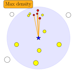
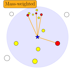
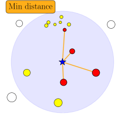
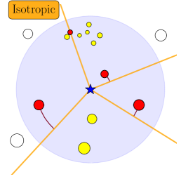
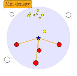
Figure 1: Five methods of gas-neighbour selection for energy injection in SN feedback, implemented in an SPH scheme. The shaded circular regions represent an SPH kernel of the stellar particle depicted by the blue star in the centre. Its gas neighbours are shown as yellow (and red) circles, whereas white circles represent gas particles outside the kernel. The size of the circles increases with decreasing density of the corresponding gas particles. We assume that the stellar particle does SN feedback by injecting four times a fixed amount of SN energy into its gas neighbours. The gas neighbours that receive this energy are coloured red (otherwise they remain yellow). Depending on the neighbour-selection method, different gas neighbours will be selected to receive the energy. We consider five cases: max_density, mass-weighted, min_distance, isotropic, and min_density (see text for details). The black arc lengths in the isotropic case (bottom left) are shown for clarity.

In this work, we quantify the importance of the way in which gas elements are selected for the injection of SN energy, and study how strongly galaxy properties are affected by the variations in gas-element-selection models. We run isolated disk galaxy simulations as well as simulations of small cosmological volumes. To the best of our knowledge, this is the first work focused on studying the effects of gas-neighbour selection. To minimize the number of free parameters, we keep the internal design of the SN feedback model fixed: in all our tests, we use the DVS12 thermal stochastic model with a fixed heating temperature and energy, and only vary the way in which gas elements are selected for SN feedback. In Section 2, we describe five algorithms – including the original one from DVS12 – of how gas particles can be chosen for receiving SN energy. In Section 3, we describe the numerical simulations used in this work. Finally, in Section 4, we present the results of the simulations, which is followed by the discussion (Section 5) and conclusions (Section 6).

2 Neighbour selection

In this section, we consider a common situation when modelling SN feedback where, in a given time-step, a star particle with $N_{\rm ngb}$ gas elements in its kernel does SN feedback by injecting energy into the surrounding gas in $N_{\rm inj}$ equal chucks, each of energy $\Delta E_{\rm inj}$. We introduce five neighbour-selection prescriptions whose purpose is to determine how the $N_{\rm inj}$ energy injections will be distributed among the $N_{\rm ngb}$ gas neighbours.

2.1 Mass-weighted method

In SPH, the most straightforward and most commonly used method for neighbour selection is to give all gas neighbours equal probabilities to be selected for SN energy injection. If there is a density gradient inside the stellar kernel, this implies that more gas neighbours will be selected for SN feedback from the denser region than from the other parts of the kernel’s volume. That is because the denser region is made up of a greater number of gas elements, which is a direct consequence of the fact that SPH is a Lagrangian method. As a result, most of the SN energy will be received by the denser gas, even though this denser gas may only comprise a small fraction of the kernel’s total volume.

From here on we will refer to this neighbour-selection method as the mass-weighted method. We also note that this is the method that was used by DVS12.

2.2 Isotropic method

To resolve the density bias outlined in §2.1, we now introduce a new neighbour-selection algorithm ensuring that the SN energy injections are statistically distributed isotropically as seen by the star.

Given a stellar particle with $N_{\rm ngb}$ gas neighbours that injects SN energy $N_{\rm inj}$ times, where each injection event is of energy $\Delta E_{\rm inj}$, we take the following steps:

1. We cast $N_{\rm rays}$ rays in different, randomly chosen (i.e. uniform probability in $\varphi$ and $\cos\theta$ in spherical coordinates) directions from the position of the star;

2. For each of the $N_{\rm rays}$ rays, we calculate great-circle distances on a unit sphere between the ray and each of the $N_{\rm ngb}$ gas neighbours by using the haversine formula

   $$\Omega_{ij}=2\arcsin\sqrt{\sin^{2}\left(\frac{\theta_{j}-\theta_{i}}{2}\right)+\cos(\theta_{i})\cos(\theta_{j})\sin^{2}\left(\frac{\varphi_{j}-\varphi_{i}}{2}\right)}\,,$$ (1)

   which uses the latitude and longitude coordinates of the ray $i$ and of the gas particle $j$ that are defined in the reference frame positioned at the stellar particle;

3. For each ray, we find the gas particle for which the arc length $\Omega_{ij}$ is minimum;

4. If the stellar particle does $N_{\rm inj}$ energy injections, where $N_{\rm inj}\leq N_{\rm rays}$, we randomly choose $N_{\rm inj}$ rays out of $N_{\rm rays}$ rays and inject the energy into the corresponding gas particles. If $N_{\rm inj}>N_{\rm rays}$, we increase $\Delta E_{\rm inj}$ by $N_{\rm inj}/N_{\rm rays}$ and inject the particles corresponding to all $N_{\rm rays}$ rays with the updated value of $\Delta E_{\rm inj}$.

2.3 Minimum distance method

Another plausible neighbour-selection model to consider is the minimum distance model (henceforth, min_distance), motivated by the idea that SN feedback needs to be as local as possible to the star. In this prescription, we sort gas neighbours according to their separations from the stellar particle. If a stellar particle has $N_{\rm inj}$ energy-injection events, then the $N_{\rm inj}$ closest gas particles will partake in the SN feedback.

Similar to the isotropic selection, the selection of the closest neighbour for SN feedback is expected to reduce the density bias seen in the mass-weighted method, albeit not always. If $N_{\rm inj}$ and $N_{\rm rays}$ are comparable to (or greater than) the number of particles in the stellar kernel, the min_distance method will turn into the mass-weighted method, while the isotropic method will remain isotropic regardless of the value of $N_{\rm inj}$.

2.4 Minimum and maximum density methods

Finally, we will examine two extreme models: minimum and maximum density (from here on, min_density and max_density). Although they are not physically motivated, in our work they will serve as an estimate of the maximum possible variation in galaxy properties due to the neighbour selection strategy. The implementation of these two density-based models is the same as in the min_distance model but in place of distance we sort gas neighbours according to their densities. In the min_density (max_density) method, if a stellar particle has $N_{\rm inj}$ energy-injection events, then the $N_{\rm inj}$ least (most) dense gas particles will receive the energy.

The five neighbour-selection algorithms that we have introduced in this section are illustrated in Figure 1. There we show five possible realisations of distributing four energy injections among the gas particles in the stellar kernel – one realisation for each neighbour-selection model. We note that in our simulations the probability of having a number of energy injections greater than one in a given time-step is much smaller than unity (see $\S$3.3.3 for more details), and in Figure 1 the value of four is chosen only to highlight the differences between the models.

3 Numerical simulations

3.1 Code and setup

To test the five neighbour-selection models described in $\S$2, we use the smoothed particle hydrodynamics astrophysical code swift (Schaller et al., 2016; Schaller et al., 2018), using the density-energy SPH scheme Sphenix (Borrow et al., 2021) to solve the hydrodynamical equations. The sphenix scheme is designed for cosmological simulations and has been demonstrated to perform well on various hydrodynamical tests on different scales (Borrow et al., 2021). We use the same SPH parameter values as in Borrow et al. (2021), including the quartic spline for the SPH kernel and the Courant–Friedrichs–Lewy parameter $C_{\rm CFL}=0.2$, which sets the time-steps of gas particles. Furthermore, we do not allow the ratio between time-steps of any two neighbouring gas particles to be greater than $4$. The target SPH smoothing length in our simulations is set to $1.2348$ times the local inter-particle separation, which corresponds to an expected weighted number of gas neighbours in the kernel $N_{\rm ngb}=64.91$ for a quartic-spline kernel.

3.2 Initial conditions

3.2.1 Isolated disk galaxy

The initial conditions for the distributions of gas and stars in the galaxy are taken from Springel et al. (2005). Our model for a Milky Way-mass galaxy comprises a dark matter halo with a Hernquist (1990) potential, a total mass $M_{200}=1.37\times 10^{12}\,\rm M_{\,\odot}$, concentration $c=9.0$ and spin parameter $\lambda=0.033$. The dark-matter halo is implemented as an analytic potential (for details see Nobels et al., in preparation) with virial velocity $v_{200}$ and radius $R_{200}$ equal to $163$ km s^-1 and $223$ kpc, respectively. In this halo, we place an exponential disk of stars and gas with the total mass of $M_{\rm disk}=0.04\,M_{200}=5.48\times 10^{10}\,\rm M_{\,\odot}$. The initial gas fraction in the disk is set to $30$ per cent and the gas initially has solar metallicity, $Z_{\odot}=0.0134$ (Asplund et al., 2009). The vertical distribution of the stellar disk has a constant scale height, which is equal to $10$ per cent of the radial scale length.

The gas particle mass at our fiducial resolution is $m_{\rm gas}=10^{5}$ $\rm M_{\odot}$, corresponding to a Plummer-equivalent gravitational softening length of $0.2$ kpc. To investigate the dependence of our results on resolution, we also ran simulations of the same galaxy at resolutions of $m_{\rm gas}=1.25\times 10^{4}$ $\rm M_{\odot}$ and $m_{\rm gas}=8\times 10^{5}$ $\rm M_{\odot}$. The former corresponds to a softening of $0.1$ kpc, and the latter to $0.4$ kpc.

In order to increase the stability of the disk in the first $\approx 0.1$ Gyr of the simulations, we assigned a distribution of stellar ages to the stellar particles present in the initial conditions assuming a constant star formation rate of $10\,\rm M_{\rm\odot}$ yr^-1, which is a typical value for a young, star-forming Milky Way-mass galaxy. In this process, we only considered stellar particles whose cylindrical radius (in the disk plane) is less than $10$ kpc from the disk centre.

Table 1: Numerical simulations used in this work. Column (1) contains the names of the simulations; (2) $N_{\rm part}$ is the number of SPH particles in the simulation (gas + stars); (3) $m_{\rm gas}$ is the initial gas-particle mass; (4) $m_{\rm dm}$ is the mass of dark-matter particles (only in cosmological simulations); (5) $\varepsilon_{\rm soft,gas}$ is the Plummer-equivalent gravitational softening length for baryons; column (6) indicates whether the simulation uses an equation of state (i.e. an effective pressure floor); column (7) shows the algorithm for neighbour selection in SN feedback used in the simulation.

Name	$N_{\rm part}$	$m_{\rm gas}$ [$\rm M_{\odot}$]	$m_{\rm dm}$ [$\rm M_{\odot}$]	$\varepsilon_{\rm soft,gas}$	EOS	SN feedback
IG_M5_isotropic	$82^{3}$	$10^{5}$	–	$0.2$ pkpc	No	Isotropic
IG_M5_mass_weighted	$82^{3}$	$10^{5}$	–	$0.2$ pkpc	No	Mass-weighted
IG_M5_min_distance	$82^{3}$	$10^{5}$	–	$0.2$ pkpc	No	Minimum distance
IG_M5_min_density	$82^{3}$	$10^{5}$	–	$0.2$ pkpc	No	Minimum density
IG_M5_max_density	$82^{3}$	$10^{5}$	–	$0.2$ pkpc	No	Maximum density
IG_M5_isotropic_eos	$82^{3}$	$10^{5}$	–	$0.2$ pkpc	Yes	Isotropic
IG_M5_mass_weighted_eos	$82^{3}$	$10^{5}$	–	$0.2$ pkpc	Yes	Mass-weighted
IG_M6_isotropic	$41^{3}$	$8\times 10^{5}$	–	$0.4$ pkpc	No	Isotropic
IG_M6_mass_weighted	$41^{3}$	$8\times 10^{5}$	–	$0.4$ pkpc	No	Mass-weighted
IG_M4_isotropic	$164^{3}$	$1.25\times 10^{4}$	–	$0.1$ pkpc	No	Isotropic
IG_M4_mass_weighted	$164^{3}$	$1.25\times 10^{4}$	–	$0.1$ pkpc	No	Mass-weighted
COS_M5_isotropic	$188^{3}$	$2.26\times 10^{5}$	$1.21\times 10^{6}$	min(0.89 ckpc, 0.35 pkpc)	No	Isotropic
COS_M5_mass_weighted	$188^{3}$	$2.26\times 10^{5}$	$1.21\times 10^{6}$	min(0.89 ckpc, 0.35 pkpc)	No	Mass-weighted
COS_M5_min_distance	$188^{3}$	$2.26\times 10^{5}$	$1.21\times 10^{6}$	min(0.89 ckpc, 0.35 pkpc)	No	Minimum distance
COS_M5_min_density	$188^{3}$	$2.26\times 10^{5}$	$1.21\times 10^{6}$	min(0.89 ckpc, 0.35 pkpc)	No	Minimum density
COS_M5_max_density	$188^{3}$	$2.26\times 10^{5}$	$1.21\times 10^{6}$	min(0.89 ckpc, 0.35 pkpc)	No	Maximum density

3.2.2 Cosmological simulations

We ran a set of cosmological simulations in a periodic comoving volume of size ($6.25$ comoving Mpc)³. The initial phases for this volume were taken from the public multiscale Gaussian white noise field Panphasia (Jenkins, 2013) and are described in Schaye et al. (2015) in Table B1. All cosmological simulations were started at redshift $z=127$. We use the Planck-13 cosmology (Planck Collaboration et al., 2014): $(\Omega_{\rm m,0},\Omega_{\rm\Lambda,0},\Omega_{\rm b,0},h,\sigma_{8},n_{\rm s})=(0.307,0.693,0.04825,0.6777,0.8288,0.9611)$, where $\Omega_{\rm m,0}$, $\Omega_{\rm b,0}$, and $\Omega_{\rm\Lambda,0}$ are the current density parameters of matter, baryons, and the dark energy, respectively; $h$ is the dimensionless Hubble constant; $\sigma_{8}$ is a linear $z=0$ rms value of Gaussian density fluctuations within $8$ $h^{-1}$Mpc spheres; and $n_{s}$ is the spectral index of primordial fluctuations.

The initial numbers of gas and dark matter particles are both equal to $188^{3}$. The gas-particle mass is $m_{\rm gas}=2.26\times 10^{5}\,\rm M_{\odot}$ and the dark-matter particle mass $m_{\rm dm}=(\Omega_{\rm m,0}/\Omega_{\rm b,0}-1)\,m_{\rm gas}=1.21\times 10^{6}\,\rm M_{\odot}$. The Plummer-equivalent gravitational softening length of baryons was set to the minimum of $0.89$ comoving kpc and $0.35$ proper kpc. The softening of dark matter was set to that of the baryons multiplied by $(\Omega_{\rm m,0}/\Omega_{\rm b,0})^{1/3}$. The simulations do not include supermassive black holes.

In this work, we only present results at $z=0$. To identify haloes in the $z=0$ snapshots, we used the publicly available structure finder VELOCIraptor (Cañas et al., 2019; Elahi et al., 2019).

3.3 Subgrid model for galaxy evolution

3.3.1 Cooling and heating

Radiative gas cooling and heating are modelled using pre-computed tables from Ploeckinger & Schaye (2020) generated with the photoionization code cloudy (Ferland et al., 2017). The model of Ploeckinger & Schaye (2020) assumes the gas to be in ionization equilibrium in the presence of a modified version of the redshift-dependent, ultraviolet/X-ray background of Faucher-Giguère (2020), cosmic rays, and a local interstellar radiation field. The interstellar radiation field, the dust-to-metals ratio and the shielding length all depend on the density and temperature of the gas.

In our fiducial model for the ISM in cosmological and isolated galaxy simulations, gas particles are allowed to cool down to temperatures as low as $10$ K. Additionally, as one of the variations, we consider a case with a constant Jeans mass pressure floor as in Schaye & Dalla Vecchia (2008), $P_{\rm eos}\propto\rho_{\rm gas}^{4/3}$, normalised to temperature $T=8\times 10^{3}\,\mathrm{K}$ at density $n_{\rm H}=0.1\,\mathrm{cm}^{-3}$. We include this variation to show that our results are not a mere consequence of the very high density gradients caused by the lack of pressure floor, and because it is common practice to include a pressure floor in simulations of galaxy formation at these resolutions.

3.3.2 Star formation

To decide whether a gas particle is star-forming or not, we use a temperature-density criterion. The cold ($T\ll 10^{4}$ K ) interstellar gas phase is expected to be unstable to star formation (e.g. Schaye, 2004). Therefore, we allow gas particles to be star-forming if their temperature $T<10^{3}$ K or their density, expressed in units of hydrogen particles per cubic cm, $n_{\rm H}$, exceeds $10^{2}\,\rm cm^{-3}$. The latter condition is essential for cosmological simulations at high redshifts where low-metallicity gas may not able to cool below $\sim 10^{4}$ K at resolved densities.

In our model, star formation occurs stochastically: if a gas particle satisfies the temperature-density criterion, its star formation rate, $\dot{m}_{\rm sf}$, is computed following the Schmidt (1959) law

$$\dot{m}_{\rm sf}=\varepsilon\frac{m_{\rm gas}}{t_{\rm ff}}\,,$$ (2)

where $t_{\rm ff}=[3\uppi/(32G\rho)]^{1/2}$ is the free-fall time and $\varepsilon=0.01$ is the efficiency of star formation per free fall time. We then compute the probability of this gas particle turning into a stellar particle by multiplying $\dot{m}_{\rm sf}$ by the particle’s current time-step and dividing by its mass $m_{\rm gas}$.

3.3.3 SN feedback

For SN (type-II) feedback, we adopt the thermal stochastic subgrid model of DVS12 and use it in combination with the original, mass-weighted method or one of the four new neighbour-selection methods from $\S$2.

In simulations of galaxies with mass resolution as in our work, stellar particles represent populations of stars with a certain age, metallicity and initial mass function (IMF) $\Phi(m)$. Given the stellar IMF, the total number of stars ending their lives as core-collapse SNe per unit stellar mass can be computed as

$$n_{\rm SN}=\int_{m_{\rm min}}^{m_{\rm max}}\,\Phi(m)\,\mathrm{d}m\,,$$ (3)

where $m_{\rm min}$ and $m_{\rm max}$ are the minimum and maximum mass of stars that die as core-collapse SNe, respectively. For the Chabrier (2003) IMF with the lower and upper mass limits of $m_{\rm min}=8\,\rm M_{\odot}$ and $m_{\rm max}=100\,\rm M_{\odot}$, this gives $n_{\rm SN}=1.18\times 10^{-2}\,\rm M^{-1}_{\odot}$. The SN energy budget per stellar particle of mass $m_{\rm*}$ can thus be written as

$$\frac{E_{\rm SN,tot}}{10^{51}\,\mathrm{erg}}=n_{\rm SN}\,f_{\rm E}\,\,m_{\rm*}=f_{\rm E}\,1.18\,\times 10^{2}\,\left(\frac{m_{\rm*}}{10^{4}\,\mathrm{M_{\odot}}}\right)\,,$$ (4)

where the free parameter $f_{\rm E}$ controls how much SN energy is liberated per single SN, in units of $10^{51}$ erg. DVS12 showed that in order to minimize the overcooling losses in SN thermal feedback, gas elements need to be heated to a temperature $T$ for which the cooling time-scale $t_{\rm c}$ (of the heated gas element) is roughly a factor of $10$ greater than the sound-crossing time-scale $t_{\rm s}$ (across the heated element). More precisely, they showed that assuming (i) the gas cooling rate is dominated by Brehmsstrahlung (ii) and the gas is fully ionized and has a primordial composition with the hydrogen mass fraction $X=0.752$, the ratio $f_{\rm t}\equiv t_{\rm c}/t_{\rm s}$ can be written in the form

$$f_{\rm t}\equiv\frac{t_{\rm c}}{t_{\rm s}}=68\left(\frac{n_{\rm H}}{1\,\rm cm^{-3}}\right)^{-2/3}\left(\frac{T}{10^{7.5}\,\rm K}\right)\left(\frac{m_{\rm ngb}}{10^{7}\,\rm M_{\odot}}\right)^{-1/3}\,,$$ (5)

where $n_{\rm H}$ is the (hydrogen) number density of the local gas and $m_{\rm ngb}$ is the total mass in the gas elements neighbouring the stellar particle (if the star has $N_{\rm ngb}$ gas neighbours, all of which are of mass $m_{\rm gas}$, then $m_{\rm ngb}=N_{\rm ngb}\,m_{\rm gas}$). The energy corresponding to a temperature increase $\Delta T$ of one such element (a particle or cell) of mass $m_{\rm gas}$ is

$$\Delta E_{\rm inj}(m_{\rm gas},\Delta T) =\frac{k_{\mathrm{B}}\Delta T}{(\gamma-1)}\frac{m_{\rm gas}}{\mu m_{\mathrm{p}}}$$

$$=1.3\times 10^{53}\,\mathrm{erg}\,\left(\frac{m_{\rm gas}}{10^{4}\,\rm M_{\odot}}\right)\left(\frac{\Delta T}{\mathrm{10^{7.5}\,K}}\right)\,,$$ (6)

where $\gamma=5/3$ is the ratio of specific heats for an ideal monatomic gas, $k_{\mathrm{B}}$ is the Boltzmann constant, $m_{\mathrm{p}}$ is the proton mass, and $\mu=0.6$ is the mean molecular weight of fully ionized gas. If a stellar particle injects its neighbours with energy $\Delta E_{\rm inj}$ and all gas elements have mass $m_{\rm gas}$, then on average this stellar particle will have

$$\langle N_{\rm inj,tot}\rangle(m_{*},f_{\rm E},m_{\rm gas},\Delta T) =\frac{E_{\rm SN,tot}(m_{*},f_{\rm E})\,}{\Delta E_{\rm inj}(m_{\rm gas},\Delta T)}$$

$$=0.91\,f_{\rm E}\,\,\left(\frac{m_{\rm*}}{m_{\rm gas}}\right)\,\left(\frac{\Delta T}{\mathrm{10^{7.5}\,K}}\right)^{-1},$$ (7)

energy injections over its lifetime. Based on equations (5) and (7), DVS12 concluded that the optimal heating temperature should be around $\Delta T=10^{7.5}$ K: making $\Delta T$ lower will decrease $f_{\rm t}$ resulting in a weaker SN feedback and stronger overcooling losses, while making $\Delta T$ significantly higher will cause undersampling of SNe feedback events (on average much less than one heating event per stellar particle).

The probability that a star particle of age $t_{j}$ heats a particular gas neighbour in a time interval from $t_{j}$ to $t_{j}+\Delta t_{j}$ can be written as

$$p_{\rm heat}(m_{\rm ngb},\Delta T,t_{j},\Delta t_{j})=\frac{\Delta E_{\mathrm{SN},j}(t_{j},\Delta t_{j})}{\Delta E_{\rm inj}(m_{\rm ngb},\Delta T)}\,,$$ (8)

where $\Delta E_{\mathrm{SN},j}$ is the SN energy released during the time interval of length $\Delta t_{j}$ and $\Delta E_{\rm inj}(m_{\rm ngb},\Delta T)$ is the energy needed to heat the total gas mass in the stellar kernel, $m_{\rm ngb}$, by a temperature $\Delta T$. The energy $\Delta E_{\mathrm{SN},j}$ is related to the total SN energy budget carried by the star particle $E_{\rm SN,tot}$ via

$$E_{\rm SN,tot}=10^{51}\,\mathrm{erg}\,f_{\rm E}\,\,m_{\rm*}\,\sum_{j}\,\int_{m_{\rm d}(t_{j}+\Delta t_{j})}^{m_{\rm d}(t_{j})}\,\Phi(m)\,\mathrm{d}m\equiv\sum_{j}\,\Delta E_{\mathrm{SN},j}\,,$$ (9)

where the function $m_{\rm d}(t)$ gives the mass of the star(s) dying as core-collapse SNe at age $t$ and in this work is computed using the metallicity-dependent stellar-lifetime tables from Portinari et al. (1998). The values of the function $m_{\rm d}(t)$ are limited to the range $m_{\rm min}\leq m_{\rm d}(t)<m_{\rm max}$, which is a consequence of the adopted IMF. As a result, the integral in the sum in equation (9) is non-zero only when the stellar age $t_{j}$ is roughly within $3\,\mathrm{Myr}\leq t_{j}<40\,\mathrm{Myr}$, where the two numbers are the (rounded) lifetimes of stars with initial masses of $m_{\rm max}$ and $m_{\rm min}$, respectively. The number of terms in the sum in equation (9) depends on the size of star particles’ time-steps.

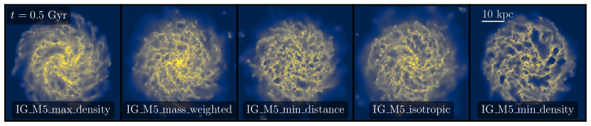
Figure 2: The distribution of gas in the isolated galaxy simulations with resolution $m_{\rm gas}=10^{5}\,\rm M_{\odot}$ shown face-on (top) and edge-on (bottom) at time $t=0.5$ Gyr, for five methods of selecting gas particles neighbouring young stellar particles for SN feedback. The colour indicates gas surface density. The efficiency of SN feedback – which differs solely due to the variations in the neighbour selection approach – increases from left to right. In the runs with more efficient SN feedback, the gas is more dispersed and the gas surface densities are on average lower.

Finally, to compute the number of thermal energy injection events $N_{\rm inj}$ in this time-step, the following algorithm is employed:

1. For a given stellar particle with available energy $\Delta E_{\mathrm{SN},j}$ and $N_{\rm ngb}$ gas neighbours comprising a total mass $m_{\rm ngb}$, the heating probability $p_{\rm heat}$ is calculated following equation (8) and $N_{\rm inj}$ is initialised with $0$;

2. For each gas neighbour out of $N_{\rm ngb}$, a random number is drawn from a uniform distribution $0\leq r<1$;

3. If the random number is smaller than $p_{\rm heat}$, then the value of $N_{\rm inj}$ is incremented by one.

After having computed $N_{\rm inj}$, we pass it to the neighbour-selection algorithm used in the simulation and follow the remaining steps as described in $\S$2 for the selected algorithm. We always use an SN energy fraction $f_{\rm E}=2.0$ , which corresponds to $2\times 10^{51}$ erg per SN, and the target heating temperature $\Delta T_{\rm SN}=10^{7.5}$ K. According to equation (7), with such parameters the expected number of thermal-injection events over the lifetime of a stellar particle is $\approx 1.8$ (and per time-step the expected number of events is $\ll 1$). We therefore use a maximum number of $N_{\rm rays}=5$ rays per stellar particle in order to never run out of rays even in the most unlikely scenarios. By running additional tests (not presented here), we verified that as long as the average number of heating events per time step per particle remains below or similar to one, our results also remain valid for a factor-of-a-few higher and lower values of $f_{\rm E}$ and $\Delta T_{\rm SN}$.

Besides heating gas to high temperatures, massive stars also enrich their surroundings with metals. In our simulations, the enrichment is done continuously following Wiersma et al. (2009) and Schaye et al. (2015).

For simplicity, we do not include SN type-Ia-related processes (energy feedback and metal enrichment), which would have negligible impact on our results.

3.3.4 Early stellar feedback

We use BPASS (Eldridge et al., 2017; Stanway & Eldridge, 2018) version 2.2.1 with a Chabrier (2003) initial mass function as stellar evolution model for all early feedback processes. The minimum and maximum stellar masses are $0.1\,\rm M_{\odot}$ and $100\,\rm M_{\odot}$, respectively. The early stellar-feedback processes we include in the simulations are stellar winds, radiation pressure and HII regions.

The implementation and effects of these three early feedback processes will be described in detail in Ploeckinger et al. (in preparation). Briefly, stellar winds inject cumulative momentum following the BPASS tables. This wind feedback is implemented as stochastic kicks of gas particles with a kick velocity of $50$ km s^-1. Radiation pressure is implemented in the same way as stellar winds and is based on the BPASS photon energy spectrum and the optical depth computed following Ploeckinger & Schaye (2020). Finally, young star particles stochastically ionize and heat neighbouring gas particles to $T=10^{4}$ K where the probability of becoming an HII region is a function of the gas density and BPASS ionising photon flux. Gas particles tagged as HII regions are not allowed to form stars.

3.4 Runs

All runs presented in this work are summarised in Table 1. Names of isolated galaxy runs and of cosmological runs begin with a prefix IG and COS, respectively. The name also indicates which neighbour selection model (from $\S$2) is used: isotropic, min_distance, mass-weighted, min_density, or max_density. If a run uses an effective pressure floor, we add the suffix _EOS to its name. The resolution of the isolated galaxy runs is indicated in the names via _M4, _M5, and _M6 corresponding to the gas-particle mass of $m_{\rm gas}=1.25\times 10^{4}\,\rm M_{\odot}$, $m_{\rm gas}=10^{5}\,\rm M_{\odot}$, and $m_{\rm gas}=8\times 10^{5}\,\rm M_{\odot}$, respectively. Finally, in the cosmological runs, _M5 stands for $m_{\rm gas}=2.26\times 10^{5}\,\rm M_{\odot}$, which is the only resolution we explore.

4 Results

4.1 Isolated galaxy simulations

We first show the results from the isolated galaxy simulations. Unless stated otherwise, all runs presented here have a particle mass of $m_{\rm gas}=10^{5}\,\rm M_{\odot}$ and do not use an effective pressure floor. We mainly focus on the three neighbour-selection methods: isotropic, min_distance, and mass-weighted. Additionally, we make use of the two more extreme methods, min_density and max_density. These two density-based methods together provide an estimate of the maximum variations in galaxy properties due to the neighbour selection for SN feedback.

4.1.1 Morphology

Figure 2 shows the distribution of gas in the isolated galaxy simulations at time $t=0.5$ Gyr, colour-coded by gas surface density. The five galaxies seen in the plot were evolved with our five neighbour-selection methods for SN feedback (from left to right, max_density, mass-weighted, min_distance, isotropic, min_density) and are shown face-on (top panels) and edge-on (bottom panels). The panels are arranged such that the runs with more efficient SN feedback (i.e. producing galaxies with less dense gas) – solely due to the differences in the neighbour-selection algorithms – are closer to the right of the plot. The neighbour-selection methods yielding more efficient SN feedback (min_distance, 3rd panel; isotropic, 4th panel; min_density, 5th panel) produce galaxies with more dispersed gas. In contrast, the gas in the galaxies evolved with less efficient methods (max_density, 1st panel; mass-weighted, 2nd panel) is more concentrated, with the gas surface densities in the centre and within spiral arms typically exceeding $10^{2}\,\rm M_{\odot}\,pc^{-2}$.

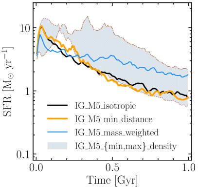
Figure 3: Star formation histories in the isolated galaxy simulations with resolution $m_{\rm gas}=10^{5}\,\rm M_{\odot}$ with isotropic (black), min_distance (orange) and mass-weighted (blue) neighbour-selection methods for SN feedback. The hatched grey area provides an estimate of the maximum variation in the star formation rate due to the neighbour-selection strategy: its boundaries are defined by the star formation rates in the runs with the most and least efficient SN feedback: IG_M5_min_density (dashed) and IG_M5_max_density (dash-dotted), respectively.

4.1.2 Star formation rates

Figure 3 displays the star formation histories for the isolated galaxy simulations with the three main neighbour-selection methods: isotropic (black), min_distance (orange), and mass-weighted (blue). For reference, we also show the runs with the two extreme models, min_density and max_density, shown as the upper and lower boundaries of the grey area. The star formation histories in IG_M5_min_density and IG_M5_max_density are further highlighted by the brown dashed and dash-dotted curves, respectively, to better distinguish the two runs. The star formation history in the IG_M5_max_density run initially ($t\lesssim 0.15$ Gyr) defines the lower boundary of the grey area, but at all later times ($t\gtrsim 0.15$ Gyr) it corresponds to the upper boundary. The opposite is true for the IG_M5_min_density run.

All three main runs experience an initial burst of star formation, which ends at $t\approx 0.15$ Gyr. The star formation rates in the isotropic and min_distance models are very much alike at all times and are systematically lower than in the mass-weighted model after the initial burst. At time $t=0.5$ Gyr, the ratio of the star formation rate in the mass-weighted model to that in the isotropic (or min_distance) is $\approx 2.0$, which increases to $\approx 2.5$ by $t=1.0$ Gyr. The stars in the IG_M5_mass_weighted run form at a higher rate because the mass-weighted method is biased towards heating gas at higher densities, where the injected SN energy dissipates faster, making the SN feedback less efficient at suppressing star formation.

Figure 4: The cumulative distribution of stellar birth gas densities (top panel) and SN feedback gas densities (bottom panel) recorded at times $0.4<t<0.6$ Gyr, in the isolated galaxy simulations with resolution $m_{\rm gas}=10^{5}\,\rm M_{\odot}$ with isotropic (black), min_distance (orange) and mass-weighted (blue) neighbour-selection methods for SN feedback. The hatched grey area is constructed in the same way as in Figure 3 (i.e. using the min_density and max_density methods). Both stellar birth densities and SN feedback densities are sensitive to the method of neighbour selection.

Comparing all five runs together, we find that star formation rates can differ by more than a factor of 5 depending on the method of neighbour selection. The max_density model is initially the most effective at suppressing star formation. That is because it targets the densest gas, where the majority of the stars form. This, however, only lasts while $t\lesssim 0.15$ Gyr after which the method becomes the least effective at preventing star formation. This is a consequence of the strongly enhanced radiative cooling losses in the densest gas where most of the SN energy is injected. The run IG_M5_min_density has the opposite behaviour: SN feedback in this run is least inefficient at suppressing the initial star formation ($t\lesssim 0.15$ Gyr), because SNe heat the least dense gas where not many stars form, but later it becomes most efficient owing to having the smallest radiative losses amongst the 5 considered runs.

4.1.3 Stellar birth densities and SN feedback densities

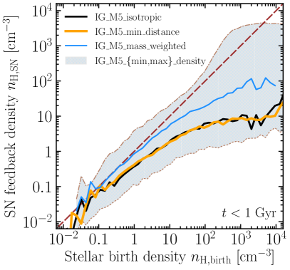
Figure 5: The median SN feedback densities versus stellar birth gas densities recorded at times $t<1$ Gyr, in the isolated galaxy simulations with resolution $m_{\rm gas}=10^{5}\,\rm M_{\odot}$ with isotropic (black), min_distance (orange) and mass-weighted (blue) neighbour-selection methods. The hatched grey area is constructed using the min_density and max_density methods. The diagonal dashed line gives the $x=y$ relation. At a fixed stellar birth density, the median SN feedback density can vary by more than two orders of magnitude depending on the method of neighbour selection.

In Figure 4, we display the cumulative distributions of stellar birth gas densities (top panel) and of SN feedback gas densities (bottom panel), which correspond, respectively, to the gas density at the time the star particle was formed and at the time the SN energy was injected. The stellar birth density distributions include all stars formed at times $0.4<t<0.6$ Gyr. For the SN gas density distributions, we used a tracer field carried by each gas particle in the simulation that would record the gas particle’s density when it was last heated by SNe; we then collected the data from all gas particles that were heated by SNe at times $0.4<t<0.6$ Gyr. The curves again show the results for the three main neighbour-selection methods, while the shaded region for min_density and max_density.

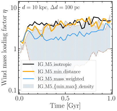
Figure 6: Gas wind mass loading factors at height $d=10\pm 0.1$ kpc above/below the galactic disk plotted versus time, in the isolated galaxy simulations with resolution $m_{\rm gas}=10^{5}\,\rm M_{\odot}$ with isotropic (black), min_distance (orange) and mass-weighted (blue) neighbour-selection methods. The hatched grey area is constructed using the min_density and max_density methods. The highest mass loading factors are attained in the min_density, isotropic and min_distance models, followed by the intermediate mass loading factors in mass-weighted, and the lowest in max_density.

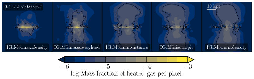
Figure 7: SN heated gas in the isolated galaxy simulations shown edge-on at $0.6$ Gyr. The colour scale indicates the mass fraction of the gas that was heated by SNe at times between $0.4$ and $0.6$ Gyr. Each panel corresponds to one of the five neighbour-selection methods for SN feedback. The black dashed contours are defined by the mass fraction of $5\times 10^{-6}$ and are shown to guide the eye. The efficiency of SN feedback and, hence, gas outflows – which differs solely due to variations in neighbour selection – increases from left to right.

Both stellar birth densities and SN feedback gas densities are sensitive to the neighbour selection, though the latter varies more significantly. In the isotropic and min_distance models, the gas turns into stars at nearly identical gas densities, which are lower than in the mass-weighted model by roughly a factor of 2. Similarly, the distributions of SN feedback gas densities look statistically identical for isotropic and min_distance and the SN densities are lower than for mass-weighted by approximately a factor of 4. The differences between min_density and max_density are more dramatic: the stellar birth densities vary by more than an order of magnitude and the feedback densities by more than two orders of magnitude.

Next, in Figure 5, we show how median SN feedback densities are correlated with stellar birth densities. For this, we made each star particle record not only the gas density at which it was born, but also the density of the gas particle it heated in its most recent SN event. Here we consider all stellar particles that had at least one SN feedback event by the end of the simulation (1 Gyr).

At low gas densities ($n_{\rm H}\lesssim 1\,\rm cm^{-3}$), the dynamical evolution of the gas is relatively slow and the density coherence length is relatively large, so that SNe go off in the ISM of roughly the same density as when the stars were formed. At higher gas densities ($n_{\rm H}\gtrsim 10\,\rm cm^{-3}$), the situation is different: the relation between stellar birth and SN feedback densities begins to flatten, which happens because high-density clumps are short-lived and/or compact. In this case, stellar particles form in clusters, which means that before a given stellar particle has its first SN thermal injection, the parent gas cloud can already be dispersed by an SN blast originated from another stellar particle. Alternatively, a star particle may move out of its birth cloud before injecting SN feedback, which will result in a lower gas density at the time of SN feedback.

The trends for the isotropic, min_distance, and mass-weighted methods converge for $n_{\rm H,birth}\lesssim 0.1\,\rm cm^{-3}$, which is a consequence of (i) little dynamical evolution of the gas between stellar-birth times and SN-feedback times, and (ii) the lack of steep density gradients at such low densities. However, at higher densities, the mass-weighted model begins to diverge from the isotropic and min_distance, which themselves again show a high degree of resemblance. At the stellar birth density of $n_{\rm H,birth}=10^{3}\,\rm cm^{-3}$, the median SN density in the isotropic and min_distance models is only $n_{\rm H,SN}\approx 10\,\rm cm^{-3}$, whereas in the mass-weighted it is $n_{\rm H,SN}\approx 10^{2}\,\rm cm^{-3}$. These SN densities are bracketed by the two more extreme models, which at $n_{\rm H,birth}=10^{3}\,\rm cm^{-3}$ have $n_{\rm H,SN}\approx 2\,\rm cm^{-3}$ (min_density) and $n_{\rm H,SN}\approx 3\times 10^{3}\,\rm cm^{-3}$ (max_density).

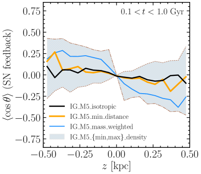
Figure 8: The average cosine of the angle between the vector from the star particle to the heated gas particle and the $z$ normal vector as a function of the height at which SN feedback occurred (see $\S$4.1.5 for details and equation 11 for the definition). If stars distributed the SN energy isotropically, then we would find $\langle\cos\theta\rangle=0$. A negative slope of $\langle\cos\theta\rangle$ with $z$ indicates a bias towards the disk. The results are shown for the isotropic (black), min_distance (orange) and mass-weighted (blue) methods. The hatched grey area is constructed using min_density and max_density. Only the gas particles that were last heated by SNe between $t=0.1$ and $1.0$ Gyr are considered. Among the five methods, isotropic gives the most isotropic distribution of the azimuthal angles, as expected.

4.1.4 Wind mass loading factors

Differences in the selection of gas neighbours also impact how effective SN feedback is at pushing gas out of the galaxy. To characterise the strength of gas outflows in isolated galaxies, we define the wind mass loading factor $\eta$ at time $t$ and at (absolute) height $d$ from the disk plane as

$$\eta(t,d,\Delta d)=\frac{1}{\dot{m}_{\rm sf,tot}}\sum_{|z_{i}\pm d|<\Delta d/2}\,\frac{m_{\mathrm{gas},i}\,|v_{z,i}|}{\Delta d}\,,$$ (10)

where $\dot{m}_{\rm sf,tot}$ is the galaxy total star formation rate at time $t$, $v_{z,i}$ is the velocity $z$ component of particle $i$, $m_{\mathrm{gas},i}$ is the mass of particle $i$, $z_{i}$ is the $z$ coordinate (height) of particle $i$ relative to the galactic disk, and the sum is computed over all outflowing (i.e. vertically moving away from the disk) gas particles whose heights are within $d\pm\Delta d/2$ from the disk (the disk plane extends in the $x$ and $y$ directions).

Figure 6 shows the temporal evolution of the mass loading factor computed at height $d=10$ kpc in a height window $\Delta d=0.1$ kpc, for the same runs as in the previous figures. It reveals that models with less (more) efficient SN feedback produce weaker (stronger) outflows, as expected. The isotropic (black curve) and min_distance (orange curve) models have a more-or-less constant mass loading factor $\eta\approx 4$. In the mass-weighted model (blue curve), the mass loading is systematically lower, $\eta\approx 2$. Furthermore, we see that in the isotropic and min_distance models, $\eta$ fluctuates around the grey area’s upper boundary, which corresponds to the IG_M5_min_density run. In other words, isotropic and min_distance methods generate galactic winds with the mass loading that is on average as high as in the run with the most efficient SN feedback. Conversely, in IG_M5_max_density, which defines the lower boundary of the grey area, SN feedback is so weak that $\eta\lesssim 1$ at all times.

To better understand the differences in $\eta$, we show in Figure 7 the galaxy edge-on at time $0.6$ Gyr, colour-coded by the mass fraction of the gas heated by SNe between $0.4$ and $0.6$ Gyr. Each panel corresponds to one of the five neighbour-selection models. The panels are arranged such that the efficiency of SN feedback (and, hence, the strength of outflows) increases from left to right. This plot is consistent with Figure 6, confirming that in runs with less (more) efficient SN feedback, the gas is less (more) outflowing. The two extreme cases are a galactic fountain-like outflow, operating at distances $|z|\lesssim 10$ kpc from the disk, in the leftmost panel (IG_M5_max_density); and the strong, stable wind, propagating beyond $|z|\approx 30$ kpc, in the rightmost panel (IG_M5_min_density).

4.1.5 Degree of isotropy of the SN feedback

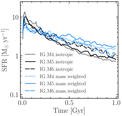
Figure 9: Star formation histories in the isolated galaxy simulations with the isotropic (black) and mass-weighted (blue) methods of neighbour selection shown at three resolutions: $m_{\rm gas}=1.25\times 10^{4}\,\rm M_{\odot}$ (M4, short-dashed), $m_{\rm gas}=10^{5}\,\rm M_{\odot}$ (M5, solid), and $m_{\rm gas}=8\times 10^{5}\,\rm M_{\odot}$ (M6, long-dashed). The differences in the star formation history between the isotropic and mass-weighted models increase with higher resolution. The isotropic and mass-weighted methods both show good convergence at our fiducial resolution M5, with the isotropic method being slightly better at times $t\gtrsim 0.5$ Gyr.

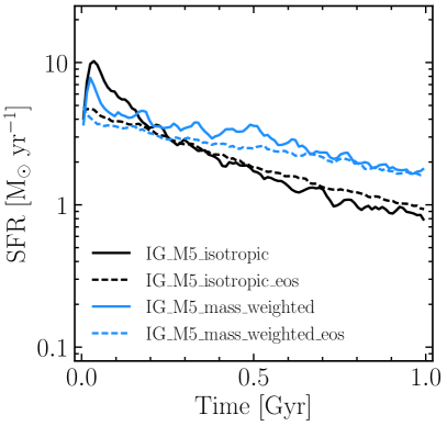
Figure 10: Star formation histories for the isolated galaxy simulations at resolution $m_{\rm gas}=10^{5}\,\rm M_{\odot}$ with the isotropic (black) and mass-weighted (blue) methods, with (dashed) and without (solid) the effective pressure floor. While the inclusion of a pressure floor slightly decreases the differences, the effect of the neighbour selection algorithm remains similar.

Our next step is to characterise the isotropy of the SN feedback. Because the galaxy has an exponentially declining density along the $z$ direction, the density gradients in this direction are particularly steep. We are interested in knowing how much better our isotropic model performs in distributing SN energy isotropically under such highly inhomogeneous conditions, compared to the other neighbour-selection algorithms.

Figure 8 shows the average cosine of the angle between the vector from the star particle to the heated gas particle and the $z$ normal vector, as a function of the height at which SN feedback events take place. More precisely, for a given $z-$coordinate bin with the two edges $z-\Delta z/2$ and $z+\Delta z/2$, the average cosine is computed as

$$\langle\cos\theta\rangle(z)=\frac{1}{N_{\rm tot}}\sum_{|\boldsymbol{r}_{\mathrm{star},i}\cdot\boldsymbol{n}_{z}-z|<\Delta z/2}\frac{(\boldsymbol{r}_{\mathrm{gas},i}-\boldsymbol{r}_{\mathrm{star},i})\cdot\boldsymbol{n}_{z}}{|\boldsymbol{r}_{\mathrm{gas},i}-\boldsymbol{r}_{\mathrm{star},i}|}\,$$ (11)

where $N_{\rm tot}$ is the number of particles satisfying the condition $|\boldsymbol{r}_{\mathrm{star},i}\cdot\boldsymbol{n}_{z}-z|<\Delta z/2$, $\boldsymbol{r}_{\mathrm{gas},i}$ is the coordinate of the $i^{\rm th}$ gas particle at the time when it was heated by SNe, $\boldsymbol{r}_{\mathrm{star},i}$ is the coordinate of the stellar particle that heated the $i^{\rm th}$ gas particle, also recorded at the time of the SN feedback event; and $\boldsymbol{n}_{z}$ is the unit vector pointing in the $z$ direction, perpendicular to the disk plane.

The results are shown for the isolated galaxy simulations with resolution $m_{\rm gas}=10^{5}\,\rm M_{\odot}$ with the isotropic (black), min_distance (orange) and mass-weighted (blue) neighbour-selection algorithms; and the grey shaded region is again defined using the IG_M5_min_density and IG_M5_max_density runs. We only consider those gas particles that were last heated by SNe between $t=0.1$ Gyr and $1.0$ Gyr; we do not include the initial evolutionary stage ($t<0.1$ Gyr) because the galaxy at such early times has a dearth of gas particles below and above the disk and because we have seen that this phase is strongly affected by the initial set-up.

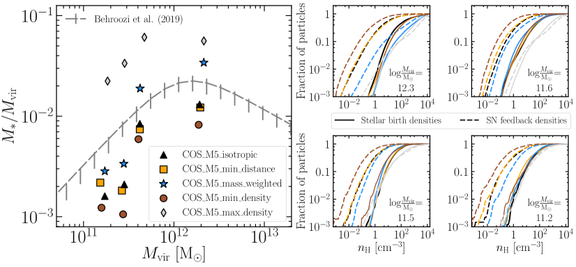
Figure 11: Left: Stellar-to-halo mass ratio versus halo mass shown for the four most massive central galaxies at $z=0$ in cosmological simulations of (6.25 cMpc)³ volume at a gas mass resolution $m_{\rm gas}=2.2\times 10^{5}\,\rm M_{\odot}$, with five different ways of selecting gas particles that receive SN energy (colour-coded). The relation from the empirical model of Behroozi et al. (2019) is shown for reference only. Right: Each smaller panel shows the cumulative distributions of stellar birth densities (solid) and SN feedback densities (dashed) for one of the four most massive galaxies from the left panel, for the same five methods of neighbour selection (colour-coding is the same as in the left panel). Consistently, the min_density (max_density) method yields the lowest (highest) stellar masses and the lowest (highest) feedback densities.

An ideal isotropic distribution would yield $\langle\cos\theta\rangle(z)=0.0$, while a negative slope with $z$ indicates a bias towards the disk. We see that among the three main runs, the isotropic model is closest to the ideal scenario, while the mass-weighted is farthest. The reason that the isotropic model also gives a slightly biased distribution is numeral sampling: if certain angular directions lack gas neighbours, there is no way that SN energy is injected there. In appendix A we show that the isotropic model approaches the ideal isotropic distribution even more closely with increasing resolution (and, hence, better sampling).

It should not be surprising that the distribution of the azimuthal angles in the min_distance model is also not too far off from $\langle\cos\theta\rangle(z)=0.0$. By always selecting the closest gas neighbour for SN heating, we reduce the impact of density gradients within the SPH kernel, and hence the bias towards excessively injecting SN energy at higher densities. This reduction in the bias increases the likelihood that the closest neighbour can exist in any angular direction (relative to the star particle), which makes the model look more isotropic. This is also partly the reason why in the previous plots, the differences between min_distance and isotropic were much smaller than between mass-weighted and isotropic. One of the statistics where min_distance does (by construction) stand out from both isotropic and mass-weighted is the distribution of distances between star particles and their heated gas neighbours (see appendix B).

4.1.6 Resolution effects

In Figure 9, we explore the impact of resolution on the variations in star formation rates caused by the differences in the adopted neighbour-selection algorithm. For clarity, we compare only the isotropic and mass-weighted models (the min_distance model is again nearly indistinguishable from isotropic). We vary the resolution in the simulations by increasing and decreasing the gas-particle mass by a factor of $8$ relative to its fiducial value of $m_{\rm gas}=10^{5}\,\rm M_{\odot}$.

The difference in the star formation histories between the isotropic and mass-weighted methods decreases with decreasing resolution and nearly disappears for $m_{\rm gas}=8\times 10^{5}\,\rm M_{\odot}$. This is a direct consequence of the overall smoother distribution of gas at the lower resolution. The isotropic and mass-weighted methods both exhibit good convergence at our fiducial resolution $m_{\rm gas}=10^{5}\,\rm M_{\odot}$ (relative to the higher, $m_{\rm gas}=1.25\times 10^{4}\,\rm M_{\odot}$ resolution), although the isotropic model converges slightly better at late times, $t\gtrsim 0.5$ Gyr.

4.1.7 Impact of an effective pressure floor

In Figure 10, we show the impact of including an effective pressure floor $P_{\rm eos}\propto\rho_{\rm gas}^{4/3}$, which is normalised at density $n_{\rm H}=0.1\,\mathrm{cm}^{-3}$ to a temperature $T=8\times 10^{3}\,\mathrm{K}$. We plot galaxy star formation rates versus time, with (dashed) and without (solid) the effective pressure floor for the isotropic (black) and mass-weighted (blue) neighbour-selection methods (4 runs in total).

The differences in galaxy star formation rates between the isotropic and mass-weighted models are similar in the two cases, though they are slightly smaller if the pressure floor is included. Compared to runs without a pressure floor, the two runs with the pressure floor have smoother star formation histories and lack an initial burst of star formation. All these differences are due to the pressure floor yielding a smoother gas distribution. By the end of the simulations, the star formation rate in the isotropic model is a factor of 2 lower than for the mass-weighted model, nearly independent of the presence or absence of the pressure floor.

4.2 Cosmological simulations

We complete our analysis with the results from (6.25 cMpc)³ cosmological volumes, at a gas mass resolution of $m_{\rm gas}=2.2\times 10^{5}\,\rm M_{\odot}$. In essence, these confirm that our findings from the isolated galaxy runs presented above also apply to cosmological simulations.

The left panel of Figure 11 displays stellar-to-halo mass ratios for the four most massive central galaxies at $z=0$ versus halo mass, for the cosmological simulations with five neighbour-selection methods: isotropic (black triangles), min_distance (orange squares), mass-weighted (blue stars), min_density (brown circles), and max_density (light-grey diamonds). For the halo masses we use the definition of the virial mass from Bryan & Norman (1998); our stellar masses are computed in 3D apertures of radius $30$ kpc. For reference, we also show the median $z=0$ stellar-to-halo mass ratio taken from the empirical model of Behroozi et al. (2019), with the error bars denoting the 16^th and 84^th percentiles.

Among the five runs, all galaxies – regardless of their halo mass – have the smallest (largest) stellar mass in the min_density (max_density) model, while the min_distance and isotropic methods yield very similar stellar masses. These results are consistent with those from our isolated galaxy runs. Furthermore, the stellar masses of all four galaxies in the mass-weighted model are higher than those in the isotropic and min_distance models by a factor of a few level, which is thus certainly not negligible. A similar shift in stellar masses is achieved by varying the SN energy budget by a factor of a few (see, e.g. Crain et al., 2015).

In the four right, smaller panels in the right-hand half of Figure 11, we show the cumulative distributions of stellar birth gas densities (solid) and SN feedback densities (dashed), in the four most massive galaxies from the left panel. The colour coding is the same as in the left panel. We see that the run with the min_density (max_density) algorithm, shown in brown (light-grey), has the lowest (highest) SN feedback densities in all four galaxies. As a result, SN feedback is most (least) effective in the simulation with the min_density (max_density) method and the galaxies in this model have the lowest (highest) star formation rates and, consequently, the lowest (highest) $z=0$ stellar masses. The feedback densities in the mass-weighted model are higher than those in min_distance and isotropic in all four galaxies. All these results are in line with our findings for the isolated galaxy runs (see Figure 4).

5 discussion

5.1 Comparison with previous work

As discussed in $\S$1, drastically different implementations of SN feedback are used by different research groups, including the so-called thermal, kinetic, decoupled, mechanical, stochastic, delayed-cooling and multi-phase subgrid models. Possibly because of the large differences in the internal design of the model, the effects of gas-neighbour selection in SN feedback have largely been overlooked so far. Only recently has this issue begun to receive some attention (Hopkins et al., 2018a; Smith et al., 2018; Hu, 2019).

Hopkins et al. (2018a) designed an algorithm to ensure statistical isotropy for their mechanical SN feedback model. In their algorithm, SN energy and momentum are distributed among gas elements neighbouring the stellar particle in proportion to the solid angles subtended by these elements, as seen by the star. The solid angles are estimated based on the effective surface areas shared by the star with its neighbours. Hopkins et al. (2018a) ran zoom-in simulations of a Milky Way-like galaxy at gas-mass resolution $m_{\rm gas}=7\times 10^{3}\,\rm M_{\odot}$ using the mesh-free, Lagrangian code gizmo (Hopkins, 2015) in its finite-mass mode; they compared the isotropic algorithm to a naive, grid-aligned one, typical for Cartesian grid-based codes. They found that in the latter case, the galaxy has a different morphology, with a disk that is significantly more compact, and attributed this effect to the removal of angular momentum from recycling material due to the (forced) grid alignment.

Smith et al. (2018) implemented a mechanical subgrid model for SN feedback alongside the Hopkins et al. (2018a) isotropic algorithm in the moving-mesh, quasi-Lagrangian code arepo (Springel, 2010) and ran simulations of an isolated galaxy with a total mass of $10^{10}\,\rm M_{\odot}$. They showed that at a resolution of $m_{\rm gas}=2\times 10^{3}\,\rm M_{\odot}$, choice of the SPH kernel weighting instead of the isotropic algorithm can result in unphysical shells propagating through the galaxy disk, sweeping up most of its gas mass. This is because if the SPH kernel weighting is used, most of the SN momentum is injected into the disk – the region where most of the gas neighbours are – rather than perpendicular to the disk.

Hu (2019) ran simulations of dwarf galaxies at much higher resolution ($m_{\rm gas}=\rm 1\,M_{\odot}$) and used a mechanical feedback model together with the healpix tessellation library (Górski et al., 2005), which makes the injection of SN energy and momentum isotropic. In Hu (2019), the $4\uppi$ solid angle was split into $12$ healpix pixels; within each pixel, they looked for $8$ gas particles in which SN energy and momentum would be injected, therefore guaranteeing that the distribution of SN energy and momentum is isotropic at the pixel level for all possible distributions of gas neighbours. They found that the type of the injection scheme – isotropic (with healpix) or naive (without healpix) – makes negligible difference for their dwarf galaxies. Such an outcome is not necessarily in conflict with our findings (and the results from the other works) because the Hu (2019) simulations had much higher resolution allowing the adiabatic phase of SN blastwaves to be fully resolved. Additionally, compared to the Milky Way-mass galaxy used in our work, in dwarf galaxies such as one used in Hu (2019), gradients in the gas density field are generally lower and the distribution of gas particles is generally smoother and more isotropic. Under such ‘less extreme’ conditions, we expect the effects of neighbour selection to be less significant than those found in our work for the Milky Way-mass galaxy. Indeed, we have run simulations of a dwarf galaxy (not shown here) with $M_{\rm 200}=1.37\times 10^{10}\,\rm M_{\odot}$, $c=14.0$, and $m_{\rm gas}=1.6\times 10^{3}\,\rm M_{\odot}$ for the five models of neighbour selection and found that the effects of neighbour selection are strongly suppressed.

We note that our isotropic algorithm is fundamentally different from those in Hopkins et al. (2018a) and Hu (2019) because our method is based on rays, not on surface areas, healpix pixels, or solid angles; and because it is used together with the stochastic subgrid model where gas neighbours are heated individually, not with the mechanical model where all gas neighbours partake in feedback events. We emphasize that the Hopkins et al. (2018a) and Hu (2019) isotropic algorithms are superior to ours when used together with SN subgrid models like the mechanical model, in which the feedback energy is distributed among many ($N\gg 1$) gas neighbours and in all angular directions. This is mainly because our isotropic method is designed for a different class of SN models – the models such as the Schaye & Dalla Vecchia (2008) kinetic model and the DVS12 thermal model where large amounts of energy are injected into one or a handful of gas neighbours. When applied to SN models distributing feedback energy among many neighbours, our method will be subject to substantial noise due to the stochastic sampling of angular directions by the finite number of rays.

Another potential weakness of our isotropic method is that it may fail when certain angular directions lack gas neighbours, which is not the case in Hu (2019). This potential problem can be seen in Figure 8 where our isotropic method is unable to produce a fully isotropic distribution of the feedback energies, $\langle\cos\theta\rangle(z)=0$, though it closely approaches it. The chance of lacking gas neighbours can be reduced by increasing the effective number of gas neighbours within the kernel or by adopting the neighbour finding strategy from Hopkins et al. (2018a) where a star particle is allowed to inject SN energy not only into the neighbours within its own kernel but also into those gas elements that are outside the stellar kernel but whose (larger) kernels contain the star particle. Both improvements will come, however, with a certain computational cost and at low resolution may cause the SN energy to be distributed over unphysically large distances.

5.2 Extension to other hydro solvers than SPH

So far all discussion and results in this work have been presented in the context of SPH. In principle, our isotropic, ray-based algorithm from $\S$2.2 can also be implemented in meshless codes like gizmo or moving-mesh codes like arepo. In the former, like in SPH solvers, the minimum arc length (equation 1) should be computed between the rays and gas particles residing in the stellar kernel. In the latter, the arc length should be computed between the rays and the mesh-generation points of the neighbouring gas cells. We expect the qualitative results of this work to apply equally to these two set-ups. We also expect our isotropic model to look ‘more isotropic’ than in this work if the average number of neighbouring gas elements is set to be greater than the value we use ($\approx 65$). That is because more neighbouring elements increases the probability of finding a particle close to the ray, resulting in a relatively better statistical isotropy of the model.

5.3 Extension to other subgrid feedback models

The neighbour-selection methods explored in this work can be used in combination with subgrid models for SN feedback other than the DVS12 thermal stochastic model. We expect the choice of the neighbour-selection algorithm to become less important if the subgrid model is less prone to radiative cooling losses. For example, in the subgrid models that inject SN energy in kinetic form and temporarily disable hydrodynamical forces acting on the kicked gas elements, the impact of the neighbour-selection strategy should be smaller than what we find here. This is because the kicked gas elements will freely escape from the ISM – without suffering any energy losses – regardless of the density of the gas they originate from. Conversely, in kinetic subgrid models for SN feedback where the kicked gas neighbours do lose energy to radiation and where the kick directions depend on the positions of the kicked gas particles with respect to the stars, the effect of neighbour selection may be even stronger than in our tests. This is because, depending on the adopted neighbour-selection method, not only the average densities of the kicked gas particles will differ, but also the paths that these particles will follow.

We emphasize that in the tests of Smith et al. (2018), it is the difference in the kick directions that dominates the changes in galaxy properties due to the injection scheme. In contrast, the effects of neighbour selection in our work are dominated by the differences in the densities at which SN energy is deposited. Because our SN feedback is thermal and stochastic, once a large amount of energy has been injected into a given gas neighbour, it will exert an isotropic pressure and the subsequent evolution of this energy will be governed by the hydro solver, which holds regardless of the neighbour selection method used in the simulation. We note also that for hydrodynamics schemes that do not smooth the gas density locally, changes in the method of neighbour selection may be more impactful than found for the density-energy SPH used in this work.

Finally, all neighbour-selection methods from $\S$2 can be applied not only to subgrid models for SN type-II feedback but also to subgrid models for SN type-Ia feedback; subgrid models for stellar early feedback including HII regions, radiation pressure and AGB winds; and subgrid models for active galactic nucleus feedback from supermassive black holes.

6 Conclusions

Although the role of supernova feedback in simulations of galaxy formation has been studied for many years, little attention has been given to the selection of the gas elements into which the SN energy is injected. In this work, we compared five methods of gas-element selection for SN feedback using isolated disk galaxy simulations as well as cosmological simulations. We focused on investigating the impact of the choice of the gas neighbours into which the SN energy is injected and kept all other aspects of the feedback model constant. We considered the (conventional) mass-weighted neighbour-selection method, a new isotropic method, and approaches where the SN energy is injected either into the closest, most dense, or least dense gas element. We kept the SN subgrid model itself fixed and used the stochastic thermal prescription from DVS12, who originally used mass weighting to select the gas particles to heat. Our main findings are as follows:

• In the presence of density gradients, the mass-weighted neighbour-selection algorithm used in DVS12 is biased towards heating gas at higher densities, which is due to the mass-weighted nature of SPH solvers. This bias is suppressed with our new algorithm, where the SN energy is distributed among gas elements as isotropically as the numerical resolution allows (Fig. 8).

• Using isolated galaxy simulations, we showed that changes in the way that gas neighbours are selected for SN feedback leads to significant variations in the galaxy star formation rates (Fig. 3), stellar birth densities (Fig. 4), and wind mass loading factors (Fig. 6). These variations are mostly driven by the efficiency of SN feedback: this depends on the densities at which the gas is heated by SNe, which in turn is sensitive to the neighbour-selection method (Fig. 5).

• The most (least) efficient SN feedback model is the one using the min_density (max_density) algorithm, where SNe heat the least (most) dense gas, which suffers the least (most) from radiative cooling losses. The three main models – isotropic, min_distance, and mass-weighted – are all bracketed by these two extreme cases. Among the main models, mass-weighted feedback is consistently less efficient than isotropic feedback, while min_distance feedback is similarly efficient (e.g. Fig. 3, 6).

• The differences in the galaxy properties caused by the usage of different neighbour-selection algorithms increase with increasing resolution. The mass-weighted and isotropic models both show good convergence at our fiducial resolution, with the isotropic method leading to a slightly better convergence at late times (Fig. 9).

• The above results are not sensitive to whether or not a pressure floor is used in the simulation. We confirmed that our results remain valid if we impose an equation of state, $P_{\rm eos}\propto\rho_{\rm gas}^{4/3}$, normalised to temperature $T=8\times 10^{3}\,\mathrm{K}$ at density $n_{\rm H}=0.1\,\mathrm{cm}^{-3}$ (Fig. 10).

• The results from the isolated galaxy simulations remain valid in cosmological simulations. In the cosmological simulations, the highest (lowest) $z=0$ galaxy stellar masses are reached with the max_density (min_density) methods, while the stellar masses in the isotropic and min_distance models are very similar and are consistently lower than those in mass-weighted by up to a factor of a few (Fig. 11).

• Our results are broadly in line with the findings of Hopkins et al. (2018a) and Smith et al. (2018) for higher-resolution simulations.

We conclude that the effects of isotropy in the SN feedback (and the choice of the element selection algorithm in general) are very important for simulations of galaxy formation and should be given at least equal consideration as other elements of the SN feedback model.

In closing, we note that if the locality of the SN feedback is important, the min_distance method can be the preferred option, especially in light of its nearly equally good isotropic character as the (explicitly) ‘isotropic’ method. However, in the test cases presented here the number of neighbours that receive SN energy is small. From additional experiments (not presented here) we found that, as expected, the differences between isotropic and min_distance increase when the number of energy-injection events per star particle per time-step increases, with isotropic yielding more efficient feedback than min_distance. Finally, we do not advocate using the min_density and max_density methods as these are extreme choices without a good physical motivation.

Data Availability

The swift simulation code, including the implementation of the neighbour-selection methods for SN feedback explored in this work, is publicly available at http://www.swiftsim.com. The data underlying this article will be shared on reasonable request to the corresponding author.

Appendix A Degree of isotropy as a function of resolution

In Figure 12 we show the average cosine of the azimuthal angle in SN feedback defined in equation (11), plotted against the height above the disk at which SN feedback events occur. The data is taken from the isolated galaxy simulations at three different resolutions, $m_{\rm gas}=1.25\times 10^{4}\,\rm M_{\odot}$ (short-dashed), $m_{\rm gas}=10^{5}\,\rm M_{\odot}$ (solid), and $m_{\rm gas}=8\times 10^{5}\,\rm M_{\odot}$ (long-dashed) for two neighbour-selection methods, isotropic (black) and mass-weighted (blue).

As expected, the isotropic model yields a more isotropic distribution than the mass-weighted model, at all three resolutions. Moreover, the higher the resolution, the closer the isotropic model is to the ideal isotropic distribution $\langle\cos\theta\rangle(z)=0$. This trend is caused by the better sampling of the gas density field with SPH particles when the resolution increases.

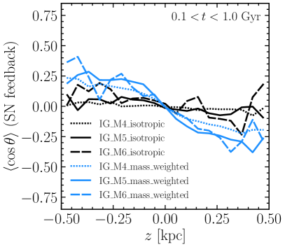
Figure 12: As Fig. 8 but for the isolated galaxy simulations with the isotropic (black) and mass-weighted (blue) neighbour selection at three different resolutions: $m_{\rm gas}=1.25\times 10^{4}\,\rm M_{\odot}$ (short-dashed), $m_{\rm gas}=10^{5}\,\rm M_{\odot}$ (solid), and $m_{\rm gas}=8\times 10^{5}\,\rm M_{\odot}$ (long-dashed). The isotropic model approaches the ideal isotropic distribution $\langle\cos\theta\rangle(z)=0$ with increasing resolution because of the better sampling of the gas density field.

Appendix B Distribution of distances between stars and their heated gas neighbours

In Figure 13 we show the probability density distribution of the distances between stellar particles and the gas neighbours they heated in their last supernova event, in the isolated galaxy simulations with resolution $m_{\rm gas}=10^{5}\,\rm M_{\odot}$ with isotropic (black), min_distance (orange) and mass-weighted (blue) neighbour-selection methods. The distances are normalised by the stellar particles SPH smoothing length at the moment of SN feedback. The SN events are selected from the time interval $0.1<t<1.0$ Gyr. For reference, we also show the probability density distribution of the form $f(x)\propto x^{2}$ (grey dashed).

We find that the probability density distributions for isotropic and mass-weighted are both very close to the shape $f(x)\propto x^{2}$. This is expected because the SPH kernel is of spherical shape so that the (average) number of gas neighbours increases as $r^{2}$ where $r$ is the distance from the kernel’s centre. The difference between mass-weighted and isotropic is only in how gas neighbours are selected based on their spherical angular coordinates. In contrast (but also as expected), the min_distance model heats gas particles at much smaller distances. The probability density distribution for min_distance peaks at the distance between stars and gas equal to $\approx 25$ per cent of the stars’ smoothing length, and goes to zero at distances exceeding $\approx 70$ per cent of the smoothing length.

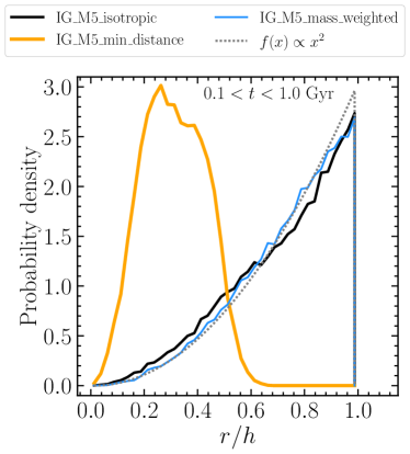
Figure 13: Probability density of the distances between stellar particles and the gas neighbours they heated in their last SN event, in units of the stellar particles’ SPH smoothing length at the moment of the feedback, in the isolated galaxy simulations with resolution $m_{\rm gas}=10^{5}\,\rm M_{\odot}$ with isotropic (black), min_distance (orange) and mass-weighted (blue) neighbour-selection methods. The SN events are selected from the time interval $0.1<t<1.0$ Gyr. The dashed grey curve gives the probability density for $f(x)\propto x^{2}$, corresponding to a radially unbiased distribution.

References

- Aguirre et al. (2001) Aguirre A., Hernquist L., Schaye J., Katz N., Weinberg D. H., Gardner J., 2001, ApJ, 561, 521
- Asplund et al. (2009) Asplund M., Grevesse N., Sauval A. J., Scott P., 2009, ARA&A, 47, 481
- Bahé et al. (2016) Bahé Y. M., et al., 2016, MNRAS, 456, 1115
- Behroozi et al. (2019) Behroozi P., Wechsler R. H., Hearin A. P., Conroy C., 2019, MNRAS, 488, 3143
- Benitez-Llambay (2015) Benitez-Llambay A., 2015, py-sphviewer: Py-SPHViewer v1.0.0, doi:10.5281/zenodo.21703, http://dx.doi.org/10.5281/zenodo.21703
- Borrow & Borrisov (2020) Borrow J., Borrisov A., 2020, Journal of Open Source Software, 5, 2430
- Borrow et al. (2021) Borrow J., Schaller M., Bower R. G., Schaye J., 2021, MNRAS,
- Bryan & Norman (1998) Bryan G. L., Norman M. L., 1998, ApJ, 495, 80
- Cañas et al. (2019) Cañas R., Elahi P. J., Welker C., del P Lagos C., Power C., Dubois Y., Pichon C., 2019, MNRAS, 482, 2039
- Chabrier (2003) Chabrier G., 2003, PASP, 115, 763
- Crain et al. (2015) Crain R. A., et al., 2015, MNRAS, 450, 1937
- Dalla Vecchia & Schaye (2008) Dalla Vecchia C., Schaye J., 2008, MNRAS, 387, 1431
- Dalla Vecchia & Schaye (2012) Dalla Vecchia C., Schaye J., 2012, MNRAS, 426, 140
- Dubois et al. (2015) Dubois Y., Volonteri M., Silk J., Devriendt J., Slyz A., Teyssier R., 2015, MNRAS, 452, 1502
- Elahi et al. (2019) Elahi P. J., Cañas R., Poulton R. J. J., Tobar R. J., Willis J. S., Lagos C. d. P., Power C., Robotham A. S. G., 2019, Publ. Astron. Soc. Australia, 36, e021
- Eldridge et al. (2017) Eldridge J. J., Stanway E. R., Xiao L., McClelland L. A. S., Taylor G., Ng M., Greis S. M. L., Bray J. C., 2017, Publ. Astron. Soc. Australia, 34, e058
- Faucher-Giguère (2020) Faucher-Giguère C.-A., 2020, MNRAS, 493, 1614
- Ferland et al. (2017) Ferland G. J., et al., 2017, Rev. Mex. Astron. Astrofis., 53, 385
- Fielding et al. (2017) Fielding D., Quataert E., Martizzi D., Faucher-Giguère C.-A., 2017, MNRAS, 470, L39
- Gatto et al. (2015) Gatto A., et al., 2015, MNRAS, 449, 1057
- Gentry et al. (2017) Gentry E. S., Krumholz M. R., Dekel A., Madau P., 2017, MNRAS, 465, 2471
- Gentry et al. (2020) Gentry E. S., Madau P., Krumholz M. R., 2020, MNRAS, 492, 1243
- Girichidis et al. (2016) Girichidis P., et al., 2016, MNRAS, 456, 3432
- Górski et al. (2005) Górski K. M., Hivon E., Banday A. J., Wandelt B. D., Hansen F. K., Reinecke M., Bartelmann M., 2005, ApJ, 622, 759
- Gutcke et al. (2021) Gutcke T. A., Pakmor R., Naab T., Springel V., 2021, MNRAS, 501, 5597
- Harris et al. (2020) Harris C. R., et al., 2020, Nature, 585, 357
- Hernquist (1990) Hernquist L., 1990, ApJ, 356, 359
- Hopkins (2015) Hopkins P. F., 2015, MNRAS, 450, 53
- Hopkins et al. (2018a) Hopkins P. F., et al., 2018a, MNRAS, 477, 1578
- Hopkins et al. (2018b) Hopkins P. F., et al., 2018b, MNRAS, 480, 800
- Hu (2019) Hu C.-Y., 2019, MNRAS, 483, 3363
- Hu et al. (2017) Hu C.-Y., Naab T., Glover S. C. O., Walch S., Clark P. C., 2017, MNRAS, 471, 2151
- Hunter (2007) Hunter J. D., 2007, Computing in Science and Engineering, 9, 90
- Jenkins (2013) Jenkins A., 2013, MNRAS, 434, 2094
- Katz (1992) Katz N., 1992, ApJ, 391, 502
- Katz et al. (1996) Katz N., Weinberg D. H., Hernquist L., 1996, ApJS, 105, 19
- Kawata (2001) Kawata D., 2001, ApJ, 558, 598
- Keller & Kruijssen (2020) Keller B. W., Kruijssen J. M. D., 2020, arXiv e-prints, p. arXiv:2004.03608
- Keller et al. (2014) Keller B. W., Wadsley J., Benincasa S. M., Couchman H. M. P., 2014, MNRAS, 442, 3013
- Kim & Ostriker (2015) Kim C.-G., Ostriker E. C., 2015, ApJ, 802, 99
- Kimm & Cen (2014) Kimm T., Cen R., 2014, ApJ, 788, 121
- Krumholz et al. (2012) Krumholz M. R., Dekel A., McKee C. F., 2012, ApJ, 745, 69
- Leroy et al. (2017) Leroy A. K., et al., 2017, ApJ, 846, 71
- Marinacci et al. (2019) Marinacci F., Sales L. V., Vogelsberger M., Torrey P., Springel V., 2019, MNRAS, 489, 4233
- McKee & Ostriker (1977) McKee C. F., Ostriker J. P., 1977, ApJ, 218, 148
- Navarro & White (1993) Navarro J. F., White S. D. M., 1993, MNRAS, 265, 271
- Oppenheimer & Davé (2006) Oppenheimer B. D., Davé R., 2006, MNRAS, 373, 1265
- Pillepich et al. (2018) Pillepich A., et al., 2018, MNRAS, 473, 4077
- Planck Collaboration et al. (2014) Planck Collaboration et al., 2014, A&A, 571, A22
- Ploeckinger & Schaye (2020) Ploeckinger S., Schaye J., 2020, MNRAS, 497, 4857
- Portinari et al. (1998) Portinari L., Chiosi C., Bressan A., 1998, A&A, 334, 505
- Roca-Fàbrega et al. (2021) Roca-Fàbrega S., et al., 2021, ApJ, 917, 64
- Rosdahl et al. (2017) Rosdahl J., Schaye J., Dubois Y., Kimm T., Teyssier R., 2017, MNRAS, 466, 11
- Scannapieco et al. (2006) Scannapieco C., Tissera P. B., White S. D. M., Springel V., 2006, MNRAS, 371, 1125
- Scannapieco et al. (2012) Scannapieco C., et al., 2012, MNRAS, 423, 1726
- Schaller et al. (2016) Schaller M., Gonnet P., Chalk A. B. G., Draper P. W., 2016, arXiv e-prints, p. arXiv:1606.02738
- Schaller et al. (2018) Schaller M., Gonnet P., Draper P. W., Chalk A. B. G., Bower R. G., Willis J., Hausammann L., 2018, SWIFT: SPH With Inter-dependent Fine-grained Tasking (ascl:1805.020)
- Schaye (2004) Schaye J., 2004, ApJ, 609, 667
- Schaye & Dalla Vecchia (2008) Schaye J., Dalla Vecchia C., 2008, MNRAS, 383, 1210
- Schaye et al. (2010) Schaye J., et al., 2010, MNRAS, 402, 1536
- Schaye et al. (2015) Schaye J., et al., 2015, MNRAS, 446, 521
- Schmidt (1959) Schmidt M., 1959, ApJ, 129, 243
- Sharma et al. (2014) Sharma P., Roy A., Nath B. B., Shchekinov Y., 2014, MNRAS, 443, 3463
- Smith et al. (2018) Smith M. C., Sijacki D., Shen S., 2018, MNRAS, 478, 302
- Springel (2010) Springel V., 2010, MNRAS, 401, 791
- Springel & Hernquist (2003) Springel V., Hernquist L., 2003, MNRAS, 339, 289
- Springel et al. (2005) Springel V., Di Matteo T., Hernquist L., 2005, MNRAS, 361, 776
- Stanway & Eldridge (2018) Stanway E. R., Eldridge J. J., 2018, MNRAS, 479, 75
- Stinson et al. (2006) Stinson G., Seth A., Katz N., Wadsley J., Governato F., Quinn T., 2006, MNRAS, 373, 1074
- Stinson et al. (2013) Stinson G. S., Brook C., Macciò A. V., Wadsley J., Quinn T. R., Couchman H. M. P., 2013, MNRAS, 428, 129
- Teyssier et al. (2013) Teyssier R., Pontzen A., Dubois Y., Read J. I., 2013, MNRAS, 429, 3068
- Valentini et al. (2017) Valentini M., Murante G., Borgani S., Monaco P., Bressan A., Beck A. M., 2017, MNRAS, 470, 3167
- Vogelsberger et al. (2013) Vogelsberger M., Genel S., Sijacki D., Torrey P., Springel V., Hernquist L., 2013, MNRAS, 436, 3031
- White & Frenk (1991) White S. D. M., Frenk C. S., 1991, ApJ, 379, 52
- Wiersma et al. (2009) Wiersma R. P. C., Schaye J., Theuns T., Dalla Vecchia C., Tornatore L., 2009, MNRAS, 399, 574
- Wiersma et al. (2011) Wiersma R. P. C., Schaye J., Theuns T., 2011, MNRAS, 415, 353