Dark Energy Survey Year 3 results: cosmological constraints from the analysis of cosmic shear in harmonic space

Abstract

We present cosmological constraints from the analysis of angular power spectra of cosmic shear maps based on data from the first three years of observations by the Dark Energy Survey (DES Y3). The shape catalog contains ellipticity measurements for over 100 million galaxies within a footprint of 4143 square degrees. Our measurements are based on the pseudo-$C_{\ell}$ method and offer a view complementary to that of the two-point correlation functions in real space, as the two estimators are known to compress and select Gaussian information in different ways, due to scale cuts. They may also be differently affected by systematic effects and theoretical uncertainties, such as baryons and intrinsic alignments (IA), making this analysis an important cross-check. In the context of $\Lambda$CDM, and using the same fiducial model as in the DES Y3 real space analysis, we find ${S_{8}\equiv\sigma_{8}\sqrt{\Omega_{\rm m}/0.3}=0.793^{+0.038}_{-0.025}}$, which further improves to ${S_{8}=0.784\pm 0.026}$ when including shear ratios. This constraint is within expected statistical fluctuations from the real space analysis, and in agreement with DES Y3 analyses of non-Gaussian statistics, but favors a slightly higher value of $S_{8}$, which reduces the tension with the Planck cosmic microwave background 2018 results from in the real space analysis to in this work. We explore less conservative IA models than the one adopted in our fiducial analysis, finding no clear preference for a more complex model. We also include small scales, using an increased Fourier mode cut-off up to $k_{\rm max}=$5\text{\,}\mathrm{\mathit{h}}\text{\,}{\mathrm{Mpc}}^{-1}$$, which allows to constrain baryonic feedback while leaving cosmological constraints essentially unchanged. Finally, we present an approximate reconstruction of the linear matter power spectrum at present time, which is found to be about 20% lower than predicted by Planck 2018, as reflected by the lower $S_{8}$ value.

1 Introduction

Gravitational lensing by the large-scale structure coherently distorts the apparent shapes of distant galaxies. The measured effect, cosmic shear, is sensitive to both the geometry of the Universe and the growth of structure, making it, in principle, a powerful tool for probing the origin of the accelerated expansion of the Universe and, consequently, the nature of dark energy. After the first detections two decades ago (Wittman et al., 2000; Kaiser et al., 2000; Van Waerbeke et al., 2000; Bacon et al., 2000), methodological advances in measurement algorithms were permitted by newly collected data, e.g. from the Deep Lens Survey (DLS, Wittman et al., 2002; Jee et al., 2013, 2016), the COSMOS survey (Scoville et al., 2007), the Canada-France-Hawaii Telescope Legacy Survey (CFHTLS, Semboloni et al., 2006) and Canada-France-Hawaii Telescope Lensing Survey (CFHTLenS, Joudaki et al., 2017) and the Sloan Digital Sky Survey (SDSS, Huff et al., 2014). These were fostered by community challenges (see, e.g., Heymans et al., 2006; Massey et al., 2007; Bridle et al., 2009; Kitching et al., 2012; Mandelbaum et al., 2014). Ongoing surveys, such as the Dark Energy Survey (DES, Flaugher, 2005), the ESO Kilo-Degree Survey (KiDS, de Jong et al., 2013; Kuijken et al., 2015), and the Hyper Suprime-Cam Subaru Strategic Program (HSC, Aihara et al., 2018a, b), have produced data sets capable of achieving cosmological constraints that are competitive with cosmic microwave background observations on the amplitude of structure, $\sigma_{8}$, and the density of matter, $\Omega_{\rm m}$, through the parameter combination $S_{8}\equiv\sigma_{8}\sqrt{\Omega_{\rm m}/0.3}$ (Troxel et al., 2018; Hikage et al., 2019; DES Collaboration, 2022; Hamana et al., 2020; Planck Collaboration et al., 2020; Asgari et al., 2021). These surveys are paving the way for the next generation of surveys, namely the Vera Rubin Observatory Legacy Survey of Space and Time (LSST, Ivezić et al., 2019), the ESA satellite Euclid (Laureijs et al., 2012), and NASA’s Nancy Grace Roman Space Telescope (Akeson et al., 2019), which will improve upon current observations in quality, area, depth and spectral coverage, in the hope of better determining the nature of dark energy. However, the level of precision needed to fully exploit the cosmological information contained in these future observations pushes the community to dissect every component of the analysis framework, from data collection to inference of cosmological parameters.

The two-point statistics of the cosmic shear field are most commonly used to extract cosmological information. While it is well known that the shear or convergence fields are, to some extent, non-Gaussian (Springel et al., 2006; Yang et al., 2011), i.e. that there is information in higher-order statistics (e.g. in peaks, Dietrich & Hartlap 2010; Martinet et al. 2018; Harnois-Déraps et al. 2021; Zürcher et al. 2021; Jeffrey et al. 2021a, or three-point functions, Takada & Jain 2003; Fu et al. 2014), the two-point functions remain the primary source of information, as they can be predicted by numerical integration of analytical models (Zuntz et al., 2015; Joudaki et al., 2017; Krause et al., 2021; Chisari et al., 2019) and efficiently measured (Jarvis, 2015). The shear two-point function can be characterized by its two components, $\xi_{+}(\theta)$ and $\xi_{-}(\theta)$, as a function of angular separation $\theta$, or by its Fourier (or harmonic) counterpart, the shear angular power spectrum, $C_{\ell}$, as a function of multipole $\ell$ (with an approximate mapping ${\ell\sim\pi/\theta}$). Both have been measured on recent data from the DES (DES Year 1, Troxel et al. 2018; Nicola et al. 2021; Camacho et al. 2021, and DES Year 3, Amon et al. 2022; Secco, Samuroff et al. 2022), KiDS (KiDS-450, Hildebrandt et al. 2017; Köhlinger et al. 2017, and KiDS-1000, Asgari et al. 2021; Loureiro et al. 2021) and HSC (Hikage et al., 2019; Hamana et al., 2020).

While, in principle, the two statistics summarize the same information, practical considerations require discarding some of the measurements for cosmological analyses via scale cuts. As a consequence, the information retained by the two statistics differs in practice, which introduces some statistical variance in cosmological constraints, on top of potential differences due to differential systematic effects. Indeed, constraints reported for the analyses of cosmic shear with KiDS-450 data showed a difference between the real- and harmonic-space analyses of $\Delta{S_{8}}=0.094$ (Hildebrandt et al., 2017; Köhlinger et al., 2017), and that of HSC Year 1 data a difference of $\Delta{\sigma_{8}}=0.28$ (Hikage et al., 2019; Hamana et al., 2020; Hamana et al., 2022), both corresponding to about $2\sigma$ discrepancies (see also fig. 11, discussed below). More recently, the comparison between three different estimators presented for KiDS-1000 data, on the other hand, showed excellent agreement (Asgari et al., 2021), including a newly developed pseudo-$C_{\ell}$ estimator in Loureiro et al. (2021). In a preparatory study (Doux et al., 2021), we quantified this effect for DES Y3 by means of simulations and showed (i) that the difference on the $S_{8}$ parameter is expected to fluctuate by about $\sigma(\Delta{S_{8}})\sim$0.02$$ for typical scale cuts, and (ii) that the observed difference is the result of the interplay between scale cuts and systematic effects, and how these impact each statistic.

In this work, we present measurements of (tomographic) cosmic shear power spectra measured from data based on the first three years of observations by the Dark Energy Survey (DES Y3), which we use to infer cosmological constraints on the $\Lambda$CDM model. We then extend our analysis and vary scale cuts to derive constraints on intrinsic alignments and baryonic feedback at small scales, the two largest astrophysical sources of uncertainty on cosmic shear studies (Chisari et al., 2018; Mandelbaum, 2018; Secco et al., 2022). Finally, we study the consistency of these constraints with those inferred from other DES Y3 weak lensing analyses, using two-point functions (Amon et al., 2022; Secco, Samuroff et al., 2022) and non-Gaussian statistics (Zürcher et al., 2022; Gatti et al., 2021b).

The paper is organized as follows: section 2 presents DES Y3 data; section 3 introduces the formalism relevant to the estimation of cosmic shear power spectra and the cosmological model, including systematic effects, intrinsic alignments and baryonic feedback; section 4 highlights the different tests we performed to validate both the measurement and modeling pipelines, some of which rely on simulations (Gaussian, $N$-body and hydrodynamical); section 5 details the three-step blinding procedure we adopted in this work; section 6 presents our main results, i.e. cosmological constraints inferred from the analysis of DES Y3 cosmic shear power spectra, and compares them to other weak lensing studies; and finally section 7 summarizes our results.

2 Dark Energy Survey Year 3 data

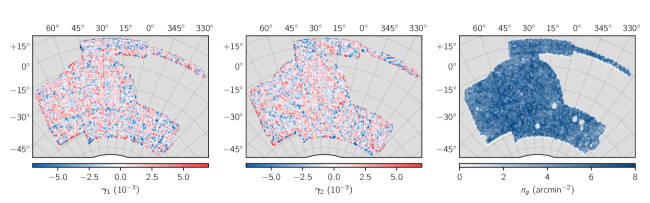
Figure 1: Maps of the two shear components, $\gamma_{1}$ and $\gamma_{2}$, and density, $n_{g}$, of the full DES Y3 weak lensing catalog.

The Dark Energy Survey The Dark Energy Survey Collaboration (DES, 2005) is a photometric imaging survey that covers around 5000 square degrees of the southern hemisphere in five optical and near-infrared bands ($grizY$). Its observations were carried out at the Cerro Tololo Inter-American Observatory (CTIO) in Chile, using the 570-megapixel DECam camera mounted on the Blanco telescope (Flaugher et al., 2015), during a six-year campaign (2013-2019). This work is based on data collected during the first three years (Y3) of observations, in particular the DES Y3 weak lensing shape catalog presented in Gatti, Sheldon et al. (2021c), which is a subsample of the Y3 Gold catalogue (Sevilla-Noarbe et al., 2021), and the inferred redshift distributions presented in Myles, Alarcon et al. (2021).

2.1 Shape catalog

Galaxy shape calibration biases are usually parameterized in terms of multiplicative and additive components. The DES Y3 shape measurements are based on the Metacalibration algorithm, which allows to self-calibrate most shear multiplicative biases, including selection effects, by measuring the response of the shape measurement pipeline to an artificial shear (Sheldon & Huff, 2017; Huff & Mandelbaum, 2017). The residual multiplicative biases, at the $23$% level, are dominated by shear-dependent detection and blending effects, and the correction was measured on a suite of realistic, DES-Y3-like image simulations presented in MacCrann et al., (2022).

The shape catalog was validated by a series of (null) tests presented in Gatti, Sheldon et al. (2021c) and found to be robust to both multiplicative and additive biases. The fiducial DES Y3 catalog used here comprises ellipticity measurements for $100\,204\,026$ galaxies, with inverse-variance weights based on signal-to-noise ratio and size. The effective area of the sample is $4143\text{\,}{\mathrm{deg}}^{2}$ (see Sevilla-Noarbe et al., 2021, for details), corresponding to an effective density of ${\bar{n}=$5.59\text{\,}\mathrm{g}\mathrm{a}\mathrm{l}\mathrm{/}\mathrm{a}\mathrm{r}\mathrm{c}\mathrm{m}\mathrm{i}\mathrm{n}\mathrm{{}^{2}}$}$. Figure 1 shows the two ellipticity components and the density of the entire sample. We will construct similar maps for each of the four tomographic bin (see next section) and use them to measure cosmic shear power spectra.

2.2 Redshift distributions

The DES Y3 shape catalogue was further divided into four tomographic bins, based on photometric redshifts inferred with the Sompz algorithm (phenotypic redshifts with self-organizing maps, Buchs et al., 2019). The DES Y3 implementation is detailed in Myles, Alarcon et al. (2021) and connects DES wide-field photometry to 1. deep-field observations (Hartley, Choi et al., 2022), using image injection with the Balrog software (Everett et al., 2022), and to 2. external spectroscopic and high-quality photometric samples, to calibrate redshifts. This Bayesian framework allows to consistently sample the posterior distribution of the four redshift distributions, while propagating calibration and sample uncertainties. Given an ensemble of realizations, uncertainties can be marginalized-over during sampling by means of the HyperRank method (Cordero, Harrison et al., 2022). The initial ensemble that was generated for DES Y3 was subsequently filtered using constraints on redshifts from cross-correlations with spectroscopic samples, as detailed in Gatti, Giannini et al. (2022). The residual uncertainty on the mean redshift of each tomographic bin is of order $\sigma_{\expectationvalue{z}}\sim 0.01$. Redshift distributions are shown in the upper panel of fig. 2, where, for each bin, the ensemble mean is represented by a solid line, and the ensemble dispersion is represented by the light bands. The lensing efficiency functions corresponding to the mean distributions at the fiducial cosmology are shown in the lower panel.

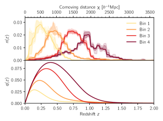
Figure 2: Redshift distributions (top) and corresponding lensing efficiency functions (bottom) for the four tomographic bins. The upper panel shows the mean (solid lines), $\pm 1\sigma$ and $\pm 2\sigma$ (light bands) percentiles of the ensemble of redshift distributions (Myles, Alarcon et al., 2021; Gatti, Giannini et al., 2022).

3 Methods

In this work, we aim at extracting cosmological constraints from the measurements of the angular auto- and cross-power spectra of the tomographic cosmic shear fields inferred from DES Y3 data. This section describes the estimation of angular spectra from data and the multivariate Gaussian likelihood model, including theoretical predictions for power spectra and their covariance matrix.

3.1 Angular power spectrum measurements

Cosmic shear is represented by a spin-2 field $\bm{\gamma}\equiv(\gamma_{1},\gamma_{2})$ on the sphere that describes, to linear order, the distortions of the ellipticities of background galaxies. A pixelized representation of the cosmic shear field can therefore be obtained by computing the weighted average of the observed ellipticities ${\mathbf{e}\equiv(e_{1},e_{2})}$ of galaxies within pixels on the sphere. For each pixel $p$ at angular position $\bm{\theta}_{p}$, we thus compute

$$\hat{\bm{\gamma}}\quantity(\bm{\theta}_{p})=\frac{\sum_{i\in p}w_{i}\mathbf{e}_{i}}{\sum_{i\in p}w_{i}},$$ (1)

where the sums run over galaxies, indexed by $i$ and with inverse-variance weight $w_{i}$, that fall into pixel $p$. The two components of the shear field estimated from the full DES Y3 weak lensing sample are represented in the left and middle panel of fig. 1. For the cosmological analysis, we compute maps of the two components of the shear field for each tomographic bin using the healpy software (Górski et al., 2005; Zonca et al., 2019) with a resolution of $N_{\rm side}=1024$, following the same procedure. Note that, prior to eq. 1, observed ellipticities were corrected for additive and multiplicative biases by subtracting the (weighted) mean ellipticity (as done in Gatti, Sheldon et al. 2021c) and dividing by the Metacalibration response, both of which were computed for each bin.

We now turn to the estimation of shear power spectra. For full-sky observations, the true shear field for redshift bin $a$, ${\bm{\gamma}^{a}\equiv(\gamma_{1}^{a},\gamma_{2}^{a})}$, can be decomposed on the basis of spherical harmonics as

$$\quantity(\gamma_{1}^{a}\pm i\gamma_{2}^{a})(\bm{\theta})=-\sum_{\ell m}\quantity[E_{\ell m}^{a}\pm iB_{\ell m}^{a}]{\,}_{\pm 2}Y_{\ell m}(\bm{\theta}),$$ (2)

where ${}_{s}Y_{\ell m}$ are the spin-weighted spherical harmonics (Hikage et al., 2011). Here, we have used the decomposition of the field into $E$- and $B$-modes, i.e. its curl-free and divergence-free components. The shear power spectra are then defined by the covariance matrix of the spherical harmonic coefficients,

$$\expectationvalue{E_{\ell m}^{a}E_{\ell^{\prime}m^{\prime}}^{b*}} =C_{\ell}^{EE}\quantity(\bm{\gamma}^{a},\bm{\gamma}^{b})\delta_{\ell\ell^{\prime}}\delta_{mm^{\prime}},$$ (3)

$$\expectationvalue{E_{\ell m}^{a}B_{\ell^{\prime}m^{\prime}}^{b*}} =C_{\ell}^{EB}\quantity(\bm{\gamma}^{a},\bm{\gamma}^{b})\delta_{\ell\ell^{\prime}}\delta_{mm^{\prime}},$$ (4)

$$\expectationvalue{B_{\ell m}^{a}B_{\ell^{\prime}m^{\prime}}^{b*}} =C_{\ell}^{BB}\quantity(\bm{\gamma}^{a},\bm{\gamma}^{b})\delta_{\ell\ell^{\prime}}\delta_{mm^{\prime}},$$ (5)

which can be estimated by

$$\hat{C}_{\ell}^{EE}\quantity(\bm{\gamma}^{a},\bm{\gamma}^{b}) =\frac{1}{2\ell+1}\sum_{m}E_{\ell m}^{a}E_{\ell m}^{b*},$$ (6)

$$\hat{C}_{\ell}^{EB}\quantity(\bm{\gamma}^{a},\bm{\gamma}^{b}) =\frac{1}{2\ell+1}\sum_{m}E_{\ell m}^{a}B_{\ell m}^{b*},$$ (7)

$$\hat{C}_{\ell}^{BB}\quantity(\bm{\gamma}^{a},\bm{\gamma}^{b}) =\frac{1}{2\ell+1}\sum_{m}B_{\ell m}^{a}B_{\ell m}^{b*}.$$ (8)

Gravitational lensing, to first order, does not create $B$-modes, therefore the cosmological signal is contained within $E$-mode power spectra, and $B$-modes can be used to detect potential systematic effects in the data, such as contamination by the point spread function (PSF, see sections 4.2 and A). However, a number of effects may generate small $B$-modes power spectra (small in comparison to to $E$-mode spectra), including second-order lensing effects (e.g. Krause & Hirata 2010), clustering of source galaxies (Schneider et al., 2002), and intrinsic alignments, as is the case with the model used in our fiducial analysis (TATT, including tidal alignment and tidal torquing mechanisms, from Blazek et al., 2019, see section 3.2.3). Therefore, we preserve both components of the field and introduce the vector notation

$$\mathbf{C}_{\ell}^{ab}\equiv\matrixquantity[C_{\ell}^{EE}\quantity(\bm{\gamma}^{a},\bm{\gamma}^{b})\\ C_{\ell}^{EB}\quantity(\bm{\gamma}^{a},\bm{\gamma}^{b})\\ C_{\ell}^{BB}\quantity(\bm{\gamma}^{a},\bm{\gamma}^{b})]$$ (9)

to denote the vectors made of the two components of the shear power spectra.

The formalism introduced so far is valid for a full-sky observations. In practice, however, the cosmic shear field is only sampled within the survey footprint, at the positions of galaxies. This induces a complicated sky window function, or mask, that correlates different multipoles and biases the estimators defined in eqs. 6 and 8. We therefore estimate angular power spectra with the so-called pseudo-$C_{\ell}$ or MASTER formalism (Hivon et al., 2002) using the NaMaster software (Alonso et al., 2019) to correct for the effect of the mask. We provide a summary of the method here and refer the reader to Hikage et al. (2011) for the development of the pseudo-$C_{\ell}$ formalism for cosmic shear, to Alonso et al. (2019) for the NaMaster implementation and to Nicola et al. (2021) and Camacho et al. (2021) for recent applications of the pseudo-$C_{\ell}$ formalism with NaMaster to DES Y1 and HSC cosmic shear data.

Let $W^{a}(\bm{\theta})$ be the mask for the shear field in bin $a$, which is zero outside the survey footprint, and let us define the masked shear field ${\tilde{\bm{\gamma}}^{a}(\bm{\theta})\equiv W^{a}(\bm{\theta})\bm{\gamma}^{a}(\bm{\theta})}$. Then the cross-power spectrum of the masked fields, i.e. the pseudo-spectrum of the fields, has an expectation value given by

$$\expectationvalue{\tilde{\mathbf{C}}_{\ell}^{ab}}=\sum_{\ell^{\prime}}\textbf{{M}}_{\ell\ell^{\prime}}^{ab}\mathbf{C}_{\ell}^{ab},$$ (10)

where $\textbf{{M}}_{\ell\ell^{\prime}}^{ab}$ is the mode-coupling (or mixing) matrix of the masks, computed analytically from their spherical harmonic coefficients (see, e.g., Alonso et al. 2019 for formulæ). This matrix describes how the mask correlates different multipoles, otherwise independent for full-sky observations, as well as leakages between $E$- and $B$-modes. While this equation may not be directly inverted due to the loss of information pertaining to masking, one can define an estimator for the binned power spectrum, defined as

$$\mathbf{C}_{L}^{ab}\equiv\sum_{\ell\in L}\omega_{L}^{\ell}\mathbf{C}_{\ell}^{ab},$$ (11)

where $\omega_{L}^{\ell}$ is a set of weights defined for multipoles $\ell$ in bandpower $L$ and normalized such that ${\sum_{\ell\in L}\omega_{L}^{\ell}=1}$. We also define the mean multipole of each bin as ${\bar{L}\equiv{\sum_{\ell\in L}\omega_{L}^{\ell}\ell}}$. The binned pseudo-spectrum $\tilde{\mathbf{C}}_{L}^{ab}$ is similarly defined from the unbinned pseudo-power spectrum $\tilde{\mathbf{C}}_{\ell}^{ab}$. The estimator for the binned power spectrum is then given by

$$\hat{\mathbf{C}}_{L}^{ab}=\sum_{L^{\prime}}\quantity(\textbf{{M}}^{ab})_{LL^{\prime}}^{-1}\tilde{\mathbf{C}}_{L^{\prime}}^{ab},$$ (12)

where the binned coupling matrix is

$$\textbf{{M}}^{ab}_{LL^{\prime}}\equiv\sum_{\ell\in L}\sum_{\ell^{\prime}\in L^{\prime}}\omega_{L}^{\ell}\textbf{{M}}_{\ell\ell^{\prime}}^{ab}.$$ (13)

The successive operations of masking, binning and decoupling described by eqs. 10, 11 and 12 are generally not permutable, such that the expectation value of the estimator in eq. 12 can differ from a naive binning of the theoretical prediction for $\mathbf{C}_{\ell}^{ab}$, as in eq. 11. Instead, the estimated shear power spectra must be compared to

$$\expectationvalue{\hat{\mathbf{C}}_{L}^{ab}}=\sum_{\ell}\mathcal{F}_{L\ell}^{ab}\mathbf{C}_{L}^{ab}$$ (14)

where the bandpower windows $\mathcal{F}_{L\ell}^{ab}$ are given by

$$\mathcal{F}_{L\ell}^{ab}=\sum_{L^{\prime}}\quantity(\textbf{{M}}^{ab})_{LL^{\prime}}^{-1}\sum_{\ell^{\prime}\in L^{\prime}}\omega_{L^{\prime}}^{\ell^{\prime}}\textbf{{M}}_{\ell^{\prime}\ell}^{ab}.$$ (15)

Throughout this work, we adopt an equal-weight binning scheme (i.e. $\omega_{\ell}=1$ if ${\ell\in L}$, $0$ otherwise) with 32 square-root-spaced bins defined between multipoles ${\ell_{\rm min}=8}$ and ${\ell_{\rm max}=2048}$ (shown by the colored bars in fig. 3). This choice ensures a good balance of signal-to-noise ratio across bandpowers $L$ while remaining flexible for scale cuts at both low and high multipoles, i.e. large and small scales (in comparison to linear and logarithmic bins that are too coarse for low and high multipoles respectively). We use weighted galaxy count maps as masks, using the weights computed by the Metacalibration algorithm. This is a close approximation to inverse-variance masks since the Metacalibration weights are themselves inverse-variance weights of ellipticity measurements (see Nicola et al., 2021). The exact bandpower windows $\mathcal{F}_{L\ell}^{ab}$ for these binning and masking schemes are compared to the naive binning (i.e. top-hat) windows in fig. 3. In particular, we observe that the exact windows extend beyond the top-hat ones, with some negative terms, especially for small multipoles below $\ell\lesssim 200$.

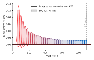
Figure 3: Bandpower window functions $\mathcal{F}_{L\ell}^{ab}$ from eq. 15. Each curve corresponds to one of the 32 bandpowers $L$ from $\ell_{\rm min}=8$ to ${\ell_{\rm max}=2N_{\rm side}=2048}$, which are equally spaced on a square-root scale throughout this work. The naive binning function is shown by the filled histogram behind.

We compute tomographic cosmic shear power spectra with NaMaster, given our binning and masking schemes, from the shear maps computed from eq. 2. These include a shape-noise component due to the intrinsic ellipticities of galaxies, which contributes an additive noise bias to the estimated auto-power spectra (whereas cross-spectra do not receive such contributions). For each tomographic bin, the noise power spectrum $N_{\ell}^{a}$ is flat for full-sky observations, and can be approximated by $N_{\ell}^{a}\approx\sigma_{e,a}^{2}/\bar{n}^{a}$, where $\sigma_{e,a}^{2}$ is the standard deviation of single-component (measured) ellipticity and $\bar{n}^{a}$ is the galaxy density in redshift bin $a$. We follow Nicola et al. (2021) and estimate the binned noise pseudo-power spectrum, which is constant, by

$$\tilde{\mathbf{N}}_{L}=\Omega_{\rm pix}\expectationvalue{\sum_{i\in p}w_{i}^{2}\frac{e_{1,i}^{2}+e_{2,i}^{2}}{2}}_{p},$$ (16)

where $\Omega_{\rm pix}$ is the pixel area in steradians (about $11.8\text{\,}\mathrm{a}\mathrm{r}\mathrm{c}\mathrm{m}\mathrm{i}\mathrm{n}\mathrm{{}^{2}}$ for ${N_{\rm side}=1024}$), and the expectation value is computed for all pixels, including those outside the survey footprint (where the value is zero). The binned noise power spectrum can then be computed with eq. 12 and subtracted from the estimated spectra. We note that this analytical estimation coincides with the expectation value of the auto-power spectra measured after applying random rotations to galaxies. Random rotations preserve the density of galaxies and the ellipticity distribution of the catalog and therefore properties of shape-noise (including its potential spatial variations), while canceling any spatial correlation (that is, both in the $E$- and $B$-modes). We also applied this procedure and verified that the result agrees with the analytical estimation, which has the advantage of being noiseless and is therefore preferred for our measurements.

We do not apply any purification of $E$- and $B$-modes (Lewis et al., 2001; Smith, 2006; Grain et al., 2009; Alonso et al., 2019) since the $B$-mode signal is largely subdominant and does not contain cosmological information, to first order. Moreover, this would require an apodization of the mask, that is speckled with empty pixels due to fluctuations in the density of source galaxies and small vetoed areas, and thus significantly decrease the effective survey area.

Finally, we correct for the effect of the pixelization of the shear fields into HealPix maps. As noted in Nicola et al. (2021), it depends on the density of galaxies, at fixed resolution: at low density, each pixel contains at most one galaxy and the map is sampling the shear field itself (but has many empty pixels), whereas at higher density, we are estimating the average of the shear field within each pixel. Here, for a resolution of $N_{\rm side}=1024$, we find that pixels with at least one galaxy contain on average $17.2$ to $17.5$ galaxies for all four tomographic bins, meaning that we are indeed sampling the averaged shear field (although a small fraction of pixels, especially on the footprint edges, have only one galaxy). This is then corrected for by dividing the pseudo-spectra $\tilde{\mathbf{C}}_{\ell}^{ab}$ by the (squared) HealPix pixel window function $F_{\ell}^{2}$, or equivalently, assigning weights $w_{L}^{\ell}=1/F_{\ell}^{2}$ for ${\ell\in L}$ for measurements (except for theoretical predictions). We test the effect of the resolution parameter in section C.1, and verify that it has negligible impact on cosmological constraints. In section 4, we validate these hypotheses and the measurement pipeline with Gaussian and $N$-body simulations.

The estimated shear power spectra for DES Y3 data are shown in fig. 4, along with the best-fit model for our fiducial $\Lambda$CDM results.

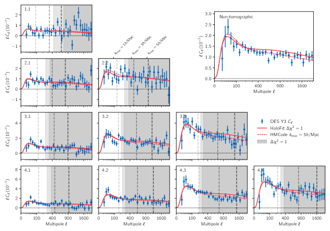
Figure 4: Cosmic shear power spectra measured from DES Y3 data. Each panel in the lower left triangle corresponds to a redshift bin pair indicated in the upper left corner. The measured $E$-mode component of the binned, noise-bias corrected power spectra is shown in blue with error bars from an analytic covariance matrix (see section 3.3). The gray shaded regions show scales that are not used in the fiducial analysis ($\Delta\chi^{2}=1$) where the effect of baryons is neglected, with extra points removed when combining with shear ratios shown in light gray (see section 3.5.1). The corresponding best-fit model within $\Lambda$CDM, discussed in section 6.1, is represented by red solid lines. The gray dashed lines show the scale cuts corresponding to $k_{\rm max}=$$135\text{\,}\mathrm{\mathit{h}}\text{\,}{\mathrm{Mpc}}^{-1}$ (see also section 3.5.2), and the corresponding best-fit model using HMCode and $k_{\rm max}=$5\text{\,}\mathrm{\mathit{h}}\text{\,}{\mathrm{Mpc}}^{-1}$$, discussed in section 6.3, is represented by red dashed lines. The upper right panel shows the measured non-tomographic shear power spectrum of DES Y3 data in blue, along with the theory expectation corresponding to the best-fit of the tomographic analysis, in red. For readability, all measurements and errors bars are scaled by the mean multipole $\bar{L}$ of each bandpower $L$, i.e. the data points show $\bar{L}\hat{\mathbf{C}}_{L}^{EE}$ and are compared to theoretical predictions of $\ell C_{\ell}$.

3.2 Modeling

In this section, we describe the theoretical model for the observed shear power spectra, including systematic uncertainties.

3.2.1 Theoretical background

Gravitational lensing deflects photons from straight trajectories and the deflection angle can be written as the gradient (on the sphere) of the lensing potential $\psi(\bm{\theta})$. In the Born approximation, the lensing potential up to comoving distance $\chi$ is given by the projection of the three-dimensional Newtonian gravitational potential $\Psi$ along the line of sight, such that

$$\psi(\bm{\theta},\chi)=2\int_{0}^{\chi}\differential{\chi^{\prime}}\frac{\chi-\chi^{\prime}}{\chi\chi^{\prime}}\Psi\quantity(\chi^{\prime}\bm{\theta},\chi^{\prime}),$$ (17)

where we assumed a flat Universe (Bartelmann, 2010). The Jacobian of the deflection angle can further be decomposed into its trace and trace-less parts, defining the spin-0 convergence field, $\kappa$, and the spin-2 shear field, $\bm{\gamma}$. Both fields can therefore be expressed in terms of second-order derivatives of the lensing potential. In the spherical harmonics representation, we have

$$\kappa =\frac{1}{4}\quantity(\eth\bar{\eth}+\bar{\eth}\eth)\psi=\frac{1}{2}\nabla_{\bm{\theta}}^{2}\psi,$$ (18)

$$\bm{\gamma} =\gamma_{1}+i\gamma_{2}=\frac{1}{2}\eth\eth\psi,$$ (19)

where $\eth$ and $\bar{\eth}$ are the raising and lowering operators of the spin-weighted spherical harmonics, ${}_{s}Y_{\ell m}$ (see Castro et al. 2005 for details and, e.g., Chang et al. 2018 for an application to curved-sky lensing mass maps). The Newtonian potential is related to the matter overdensity field $\delta$ via the Poisson equation,

$$\nabla^{2}\Psi=\frac{3\Omega_{\rm m}H_{0}^{2}}{2ac^{2}}\delta,$$ (20)

where $\Omega_{\rm m}$ is the matter density parameter, $H_{0}$ is the Hubble constant today and $a=1/(1+z)$ is the scale factor. Combining eqs. 17 and 18, we obtain

$$\kappa(\bm{\theta},\chi)=\frac{3\Omega_{\rm m}H_{0}^{2}}{2c^{2}}\int_{0}^{\chi}\frac{\differential{\chi^{\prime}}}{a(\chi^{\prime})}\frac{\chi-\chi^{\prime}}{\chi\chi^{\prime}}\delta\quantity(\chi^{\prime}\bm{\theta},\chi^{\prime}),$$ (21)

where we have added the radial component of the Laplacian of the potential, $\nabla_{\chi}^{2}\Psi$, that vanishes in the integration.

For a sample of galaxies, the observable convergence and shear fields are integrated over comoving distance and weighted by their redshift distribution $n_{a}(\chi)$, where $a$ denotes the bin index. In the Limber approximation (Limber, 1953; Kaiser, 1992, 1998; LoVerde & Afshordi, 2008), the convergence cross-power spectrum for bins $a$ and $b$ is

$$C^{\kappa_{a}\kappa_{b}}_{\ell}=\int\differential{\chi}\frac{q_{a}(\chi)q_{b}(\chi)}{\chi^{2}}P_{\rm NL}\quantity(k=\frac{\ell+1/2}{\chi},z(\chi)),$$ (22)

where the lensing efficiency is given by

$$q_{a}(\chi)=\frac{3\Omega_{\rm m}H_{0}^{2}}{2c^{2}}\frac{\chi}{a(\chi)}\int_{\chi}^{\chi_{H}}\differential{\chi^{\prime}}n_{a}(\chi^{\prime})\frac{\chi-\chi^{\prime}}{\chi^{\prime}},$$ (23)

where $\chi_{H}$ is the distance to the horizon (effectively, the comoving distance where the redshift distributions vanish). The lensing efficiency functions for DES Y3 galaxies are shown in the lower panel of fig. 2. Given eqs. 18 and 19, the cosmic shear $E$-mode power spectrum is given by

$$C^{ab}_{\ell}=T_{\ell}C^{\kappa_{a}\kappa_{b}}_{\ell},$$ (24)

where the prefactor, $T_{\ell}=(\ell+2)(\ell+1)\ell(\ell-1)/(\ell+1/2)^{4}$, is often replaced by 1, an excellent approximation for $\ell\gtrsim 10$ Kitching et al. (see 2017, for a complete discussion); Kilbinger et al. (see 2017, for a complete discussion). We verified that these two approximations are correct, given our binning scheme, with an error of at most 0.2% on the largest scales considered.

3.2.2 Non-linear power spectrum

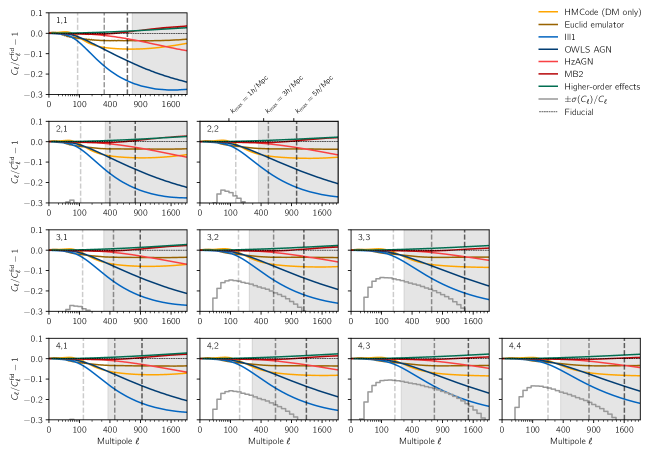
Figure 5: Residual shear power spectra with respect to the fiducial power spectra, $C_{\ell}^{\rm fid}$. The orange (HMCode) and brown (Euclid Emulator) curves show residuals for alternative prescription of the non-linear power spectrum (see section 3.2.2). The blue and red curves show the effect of baryons as predicted by

four hydrodynamical simulations (Illustris, OWLS AGN, Horizon AGN and MassiveBlack II). Higher-order lensing effects computed with CosmoLike are also shown, in green, to be small. The error bars are shown by the gray step-wise lines which represent $\pm\sigma(C_{\ell})/C_{\ell}$ on the same scale (only $-\sigma(C_{\ell})/C_{\ell}$ is visible). The gray shaded regions show scales that are not used in the fiducial analysis where the effect of baryons is neglected. The gray dashed lines show the scale cuts corresponding to $k_{\rm max}=$$135\text{\,}\mathrm{\mathit{h}}\text{\,}{\mathrm{Mpc}}^{-1}$ (see section 3.5.2).

Following the general methodology of the DES Y3 large-scale structure analysis set in Krause et al. (2021), for our fiducial model we compute the non-linear matter power spectrum $P_{\rm NL}(k,z)$ using the Boltzmann code CAMB (Lewis et al., 2000; Howlett et al., 2012) with the HaloFit extension to non-linear scales (Smith et al., 2003), with updates to dark energy and massive neutrinos from Takahashi et al. (2012). HaloFit is reported to be accurate at the 5% level for $k\leq$1\text{\,}\mathrm{\mathit{h}}\text{\,}{\mathrm{Mpc}}^{-1}$$, when compared to $N$-nody simulations, and degrading for smaller scales. However, Krause et al. (2021) showed that DES Y3 cosmic shear is insensitive to varying the prescription to model the small-scale power spectrum by substituting HaloFit for HMCode (with dark matter only), the Euclid Emulator, or the Mira-Titan Emulator (Mead et al., 2015; Euclid Collaboration et al., 2019; Lawrence et al., 2017). We show a comparison of some of these prescriptions in fig. 5 and we verify the robustness of our fiducial choice in in section 4.4.1.

3.2.3 Intrinsic alignments

Galaxies are extended objects and therefore subject to tidal forces. Their intrinsic shapes, or ellipticities, are consequently not fully random but rather tend to align with the tidal field of the gravitational potential and therefore each other (Hirata & Seljak, 2004; Bridle & King, 2007). As a consequence, the shear power spectrum estimated from galaxies receives additional contributions from the correlation of intrinsic shapes, $C_{\ell,{\rm I}{\rm I}}^{ab}$, and the cross-correlations of intrinsic shapes with the cosmological shear field, $C_{\ell,{\rm GI}}^{ab}$ and $C_{\ell,{\rm IG}}^{ab}$, such that the theoretical spectrum of the observed signal reads ${C_{\ell}^{ab}+C_{\ell,{\rm GI}}^{ab}+C_{\ell,{\rm IG}}^{ab}+C_{\ell,{\rm I}{\rm I}}^{ab}}$.

In this work, we follow the DES Y3 analysis of cosmic shear in real space (Krause et al., 2021; Amon et al., 2022; Secco, Samuroff et al., 2022) and use the so-called TATT framework (Blazek et al., 2019) as our fiducial choice to model these extra terms stemming from intrinsic alignments (IA). This model unified tidal alignment (TA) with tidal torquing (TT) mechanisms, proposed by Catelan et al. (2001); Crittenden et al. (2001); Mackey et al. (2002), thanks to a perturbative expansion of the intrinsic galaxy shape field in the density and tidal fields, up to second order in the tidal field. We refer the reader to Secco, Samuroff et al. (2022) for full details of the implementation and a justification of this choice. The TA and TT contributions are each modulated by an amplitude (respectively $A_{\rm TA}$ and $A_{\rm TT}$) and a redshift-dependence parameter (respectively $\alpha_{\rm TA}$ and $\alpha_{\rm TT}$), with an additional linear bias $b_{\rm TA}$ of sources contributing to the TA signal. The non-linear alignment model (NLA, Hirata & Seljak, 2004; Bridle & King, 2007), commonly used in cosmic shear analyses (Troxel et al., 2018; Asgari et al., 2021; Hamana et al., 2020; Hikage et al., 2019) is contained in the TATT framework and corresponds to the case $A_{\rm TT}=b_{\rm TA}=0$.

The TATT model also predicts a small, but non-zero $B$-mode power spectrum, when $b_{\rm TA}\neq 0$ or $A_{\rm TT}\neq 0$. In the main parts of the analysis, the $B$-mode spectrum is not used for cosmological analysis. Instead, it is demonstrated in section 4.2.1 that DES Y3 data is consistent with no $B$-modes, rejecting the hypothesis of a strong contamination of the signal by systematic effects that would source $B$-modes, such as leakage from the PSF, measured in section 4.2.2 and appendix A. This test thereby also excludes a detectable contribution of the IA $B$-mode signal, with the unlikely caveat that systematic effects and IA may cancel each other. In addition, the PSF test allows us to predict the contamination of $B$-mode spectra, which is found to be subdominant, by an order of magnitude, to the TATT-predicted $B$-mode signal for $A_{\rm TT}=1$, which is well within current $E$-mode constraints. Therefore, we will extend the cosmological analysis in section 6.2 and include $B$-mode measurements to improve constraints on the TATT parameters. To do so, we employ the same pseudo-$C_{\ell}$ formalism and extend the mode-coupling matrices in eqs. 10 and 14 to account for the $B$-mode component. Note that NaMaster computes both $E$ and $B$ components of the mixing matrices as well as the cross-terms accounting for leakages between the two components. The fiducial analysis simply discards those terms, as $B$-to-$E$ mode leakage is found to be negligible. However, $E$-to-$B$ mode leakage is found to significantly contribute to the $B$-mode signal, in comparison to the TATT-predicted $B$-mode signal (they are of comparable magnitude for $A_{\rm TT}$ of order unity). Therefore, the extended analysis including $B$-mode measurements uses consistent modeling of multipole coupling and $E$/$B$-mode leakage. The covariance matrix for the $B$-mode measurement as well as the cross-covariance between $E$- and $B$-mode measurements are computed from a set of $10\,000$ Gaussian simulations based on DES Y3 data, as detailed in section 4.1.1.

3.2.4 Effects of baryons

Astrophysical, baryonic processes redistribute matter within dark-matter halos and modify the matter power spectrum at small scales (Chisari et al., 2018; Schneider et al., 2019, 2020; Huang et al., 2021). Feedback mechanisms from active galactic nuclei and supernovæ heat up their environment and suppress clustering in the range $k\sim$$1\text{\,}\mathrm{\mathit{h}}\text{\,}{\mathrm{Mpc}}^{-1}10\text{\,}\mathrm{\mathit{h}}\text{\,}{\mathrm{Mpc}}^{-1}$, while cooling mechanisms enhance clustering on smaller scales. The complex physics involved in these mechanisms has been modeled in multiple hydrodynamical simulations (van Daalen et al., 2011; Dubois et al., 2014; Vogelsberger et al., 2014; Khandai et al., 2015). However the absolute and relative amplitudes of the various effects remain poorly understood and constitute a major source of uncertainty, at the level of tens of percent, on the matter power spectrum at scales $k\gtrsim$5\text{\,}\mathrm{\mathit{h}}\text{\,}{\mathrm{Mpc}}^{-1}$$, and on the shear power spectrum at multipoles as low as $\ell\gtrsim 100$, as shown on fig. 5 (see also Huang et al., 2019).

Our fiducial analysis follows the DES Y3 analysis and discards scales that are strongly affected by baryonic effects, as detailed in section 3.5.1. In general, the impact of baryons on the shear power spectrum can be computed by rescaling the matter power spectrum,

$$P_{\rm NL}(k,z)\rightarrow P_{\rm NL}(k,z)\frac{P_{\rm hydro}(k,z)}{P_{\rm DM}(k,z)},$$ (25)

where $P_{\rm hydro}(k,z)$ and $P_{\rm DM}(k,z)$ are the matter power spectra measured from hydrodynamical simulations, respectively with and without the effects of baryons. In particular, we will use four simulations, selected to provide a diverse range of scenarios: Illustris (Vogelsberger et al., 2014), OWLS AGN (van Daalen et al., 2011), Horizon AGN (Dubois et al., 2014) and MassiveBlack II (Khandai et al., 2015). We will use this approach to evaluate the impact of baryons, shown in fig. 5, and determine our fiducial set of scale cuts, in section 3.5.1.

We will later extend our analysis to smaller scales, which requires to model and marginalize over baryonic effects. To do so, we will use HMCode (Mead et al., 2015), instead of HaloFit, to simultaneously model the effects of non-linearities and baryonic feedback on the matter power spectrum. This adds one or two extra parameters, namely the minimum halo concentration $A_{\rm HM}$ and the halo bloating parameter $\eta_{\rm HM}$, which were shown to approximately follow the linear relation $\eta_{\rm HM}=1.03-0.11A_{\rm HM}$ for various simulations (see Mead et al., 2015). Although Mead et al. (2021) recently presented an updated version of HMCode with improved treatment of baryon-acoustic oscillation damping and massive neutrinos, we will only consider the 2015 version of the code, which was available at the onset of this work. We note that Tröster et al. (2021) found only a small impact of HMCode versions on cosmological constraints derived from cosmic shear and Sunyaev-Zeldovich effect cross-correlations.

3.2.5 Shear and redshift uncertainties

We include uncertainties on the shear calibration and redshift distributions following the DES Y3 real-space analysis (Krause et al., 2021; Amon et al., 2022; Secco, Samuroff et al., 2022).

In our fiducial model, uncertainties in redshift distributions are captured by allowing overall translations of the fiducial redshift distributions, shown in fig. 2, such that

$$n_{a}(z)\rightarrow n_{a}(z+\Delta z_{a}).$$ (26)

We parametrize the residual uncertainty in the shear calibration following a standard procedure which amounts to an overall rescaling of the shear signal in each redshift bin, such that

$$C_{\ell}^{ab}\rightarrow(1+m_{a})(1+m_{b})C_{\ell}^{ab}.$$ (27)

The four shear biases, $m_{a}$, are assumed to be redshift-independent within each bin. Both of these choices are approximations to the more sophisticated approaches developed over the course of the DES Y3 analysis.

For redshift uncertainties, the Sompz method provides a ensemble of redshift distributions encapsulating the full uncertainty (Myles, Alarcon et al., 2021), and not just that of the mean redshift. However, it was shown in Cordero, Harrison et al. (2022) and Amon et al. (2022) that the simpler parametrization of eq. 26 is sufficient for DES Y3, which we test in section C.1. For shear calibration, a new approach was developed alongside the image simulations presented in MacCrann et al., (2022). In short, it was shown that the redshift distribution of a sample, $n(z)$, corresponds to the response of the shear estimated from this sample to a cosmological shear signal, as a function of the redshift of the signal. In the presence of galaxy blending, the response is modified, which may be captured by an effective redshift distribution, $n_{\gamma}(z)$, normalized to $1+m$. Realistic simulations, that used the same pipelines as DES Y3 data for co-addition, detection and shear measurements, allowed to jointly estimate residual uncertainties in shear and redshift biases. These results were subsequently mapped onto the standard parametrization of eqs. 26 and 27, thus defining the priors over these parameters, as detailed in table 1. Extensive testing demonstrated that our fiducial approach is sufficiently accurate given the statistical uncertainties in DES Y3 (see MacCrann et al.,, 2022; Cordero, Harrison et al., 2022; Amon et al., 2022, for details).

3.2.6 Higher-order shear

Our modeling ignores higher-order contributions to the shear signal due to the magnification and clustering of the galaxy sample as well as the fact we can only access the reduced shear, given by $\gamma/(1-\kappa)$. These contributions are computed in Krause et al. (2021); Secco, Samuroff et al. (2022) and found to be below 5% for the scales used in this analysis, as shown by the orange curves in fig. 5. We verified that they have a negligible impact on cosmological constraints for DES Y3.

3.3 Likelihood and covariance

We assume cosmic shear spectrum measurements follow a multivariate Gaussian distribution with fixed covariance. The theoretical predictions detailed in the previous section are convolved with the bandpower windows, following eqs. 14 and 15.

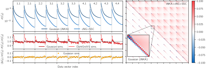
Figure 6: Features and validation of the analytical covariance matrix used in this work, computed with NaMaster and CosmoLike. Upper left: error bars given by the square-root of the diagonal of the Gaussian (dark blue) and non-Gaussian (light blue) contributions to the covariance matrix. Middle left: comparison of the error bars computed from Gaussian simulations (dark red) and DarkGridV1 simulations (light red) with the fiducial error bars. Lower left: residuals of the pseudo-$C_{\ell}$ measurements from the Gaussian simulations with respect to the input (binned) spectra. In all left panels, the horizontal axis corresponds to indices of the components stacked data vector. The corresponding redshift bin pairs are indicated at the top of the upper panel, with each block corresponding to multipoles in the range $82048$. Right: correlation matrix, with only the Gaussian contribution in the lower triangle, and both Gaussian and non-Gaussian contributions in the upper triangle (note the normalization in the range $-0.10.1$).

The covariance of $E$-mode shear power spectra is computed analytically as follows. It is decomposed as a sum of Gaussian and non-Gaussian contributions from the shear field. The Gaussian contribution is computed with NaMaster using the improved narrow-kernel approximation (iNKA) estimator developed in García-García et al. (2019) and optimized by Nicola et al. (2021). This estimator correctly accounts for mode-mixing pertaining to masking and binning, consistently with the pseudo-$C_{\ell}$ framework presented in section 3.1. It requires the mode-coupled pseudo-$C_{\ell}$ spectra, computed from the theoretical full-sky spectra convolved by the mixing matrix from eq. 10, and including noise bias for auto-spectra, computed from the data with eq. 16. These are then rescaled by the product of masks over all pixels Nicola et al. (for details, see 2021).

The non-Gaussian contribution is the sum of two terms: the connected four-point covariance (cNG) arising from the shear field trispectrum, and the so-called super-sample covariance (SSC), accounting for correlations of multipoles used in the analysis with super-survey modes. Both non-Gaussian terms are computed using the CosmoLike software (Eifler et al., 2014; Krause & Eifler, 2017), with formulae derived in Takada & Jain (2009); Schaan et al. (2014). These analytic expressions do not account for the exact survey geometry and only apply a scaling by the fraction of observed sky, $f_{\rm sky}$. Therefore, we interpolate these computations at all pairs of integer-valued multipoles and use the bandpower windows from eq. 15 to obtain an approximation of the non-Gaussian covariance terms for the binned power spectrum estimator described in the previous section. The non-Gaussian terms (cNG+SSC) are subdominant with respect to the Gaussian contribution (see the upper left panel of fig. 6) and this represents a good approximation to the extra covariance of different multipoles (i.e. off-diagonal terms), which becomes non-negligible only on the smallest scales.

Figure 6 illustrates properties of the fiducial covariance matrix, computed as explained above. First, as can be seen on the left panel, the non-Gaussian terms are largely subdominant in the computation of the error bars. Then, the right panel, showing the correlation matrix, reveals that multipole bins are largely uncorrelated in the Gaussian covariance, and only correlated at the 10% level at most due to the non-Gaussian contributions. Adjacent multipole bins are actually slightly anti-correlated due to mode coupling and decoupling, at the 6% level for the lowest bins to below 1% for the highest bins.

The covariance matrix of $B$-mode shear power spectra and the cross-covariance between $E$- and $B$-mode power spectra are computed from Gaussian simulations, presented in section 4.1.1, as the original NKA estimator was found to be unreliable for these spectra in García-García et al. (2019).

3.4 Parameters and priors

For our fiducial analysis, we vary six parameters of the $\Lambda$CDM model, namely the total matter density parameter $\Omega_{\rm m}$, the baryon density parameter $\Omega_{\rm b}$, the Hubble parameter $h$ (where ${H_{0}=$100\text{\,}\mathrm{\mathit{h}}\text{\,}\mathrm{km}\text{\,}{\mathrm{s}}^{-1}\text{\,}{\mathrm{Mpc}}^{-1}$}$), the amplitude of primordial curvature power spectrum $A_{\rm s}$ and the spectral index $n_{\rm s}$, and the neutrino physical density parameter $\Omega_{\nu}h^{2}$.

We also vary the five parameters of the intrinsic alignments model, TATT. When restricting to the NLA model, we fix ${A_{\rm TT}=\alpha_{\rm TT}=b_{\rm TA}=0}$. Our validation tests are carried out assuming the TATT model, but using the NLA best-fit values from Samuroff et al. (2019) based on DES Year 1 data, since this work found no strong preference for the more complex model.

In addition to the cosmological and astrophysical parameters described above, our analysis includes two nuisance parameters per redshift bin to account for uncertainties in shape calibration ($m_{a}$) and redshift distributions (${\Delta z_{a}}$), as described in section 3.2.5.

The full list of parameters for the baseline $\Lambda$CDM model with their priors is shown in table 1. Throughout this paper we assume the Planck 2018 (Planck Collaboration et al., 2020) best-fit cosmology derived from TT,TE,EE+lowE+lensing+BAO data as our fiducial parameter values.

In addition, we will consider alternative models that require extra varied parameters:

• When using HMCode to model small scales, we vary either $A_{\rm HM}$ only (using the relationship between $A_{\rm HM}$ and $\eta_{\rm HM}$ suggested in Mead et al., 2015), or both $A_{\rm HM}$ and $\eta_{\rm HM}$ parameters, applying uniform priors $A_{\rm HM}\sim\mathcal{U}(0,10)$ and $\eta_{\rm HM}\sim\mathcal{U}(0,2)$.

• When constraining the $w$CDM model, we vary the dark energy equation-of-state $w$, with a uniform prior in the range $[-2,-1/3]$.

Finally, we will, in some cases, include independent (geometric) information from measurements of ratios of galaxy-galaxy lensing two-point functions at small scales, as presented in Sánchez, Prat et al. (2021). Given an independent lens sample Porredon et al. (here, MagLim, presented in 2021), the ratios of tangential shear signals for two redshift bins of the source sample around the same galaxies from a common redshift bin of the lens sample depend largely on distances to these samples. Shear ratios (SR) can therefore be used to constrain uncertainties in the redshift distributions. We only exploit small-scale measurements, corresponding to scales of approximately $2\text{\,}{\mathrm{\mathit{h}}}^{-1}\text{\,}\mathrm{Mpc}6\text{\,}{\mathrm{\mathit{h}}}^{-1}\text{\,}\mathrm{Mpc}$, or $\ell_{\rm min}\sim$$3601200$ for redshift bins $14$, that are largely independent from the scales we use in this analysis (see fig. 4 and section 3.5). In these cases, we incorporate shear ratios at the likelihood level, using a Gaussian likelihood. The modeling of shear ratios necessitates extra parameters, namely the clustering biases and redshift distribution uncertainties for each of the three lens bins used here. Details about the shear-ratio likelihood and priors can be found in Sánchez, Prat et al. (2021).

Parameter	Symbol	Prior
Total matter density	$\Omega_{\rm m}$	$\mathcal{U}(0.1,0.9)$
Baryon density	$\Omega_{\rm b}$	$\mathcal{U}(0.03,0.07)$
Hubble parameter	$h$	$\mathcal{U}(0.55,0.91)$
Primordial spectrum amplitude	$A_{\rm s}\times 10^{9}$	$\mathcal{U}(0.5,5)$
Spectral index	$n_{\rm s}$	$\mathcal{U}(0.87,1.07)$
Physical neutrino density	$\Omega_{\nu}h^{2}$	$\mathcal{U}(0.0006,0.00644)$
IA amplitude (TA)	$A_{\rm TA}$	$\mathcal{U}(-5,5)$
IA redshift dependence (TA)	$\alpha_{\rm TA}$	$\mathcal{U}(-5,5)$
IA amplitude (TT)	$A_{\rm TT}$	$\mathcal{U}(-5,5)$
IA redshift dependence (TT)	$\alpha_{\rm TT}$	$\mathcal{U}(-5,5)$
IA linear bias (TA)	$b_{\rm TA}$	$\mathcal{U}(0,2)$
Photo-$z$ shift in bin 1	$\Delta z_{1}$	$\mathcal{N}(0,0.018)$
Photo-$z$ shift in bin 2	$\Delta z_{2}$	$\mathcal{N}(0,0.015)$
Photo-$z$ shift in bin 3	$\Delta z_{3}$	$\mathcal{N}(0,0.011)$
Photo-$z$ shift in bin 4	$\Delta z_{4}$	$\mathcal{N}(0,0.017)$
Shear bias in bin 1	$m_{1}$	$\mathcal{N}(-0.0063,0.0091)$
Shear bias in bin 2	$m_{2}$	$\mathcal{N}(-0.0198,0.0078)$
Shear bias in bin 3	$m_{3}$	$\mathcal{N}(-0.0241,0.0076)$
Shear bias in bin 4	$m_{4}$	$\mathcal{N}(-0.0369,0.0076)$

Table 1: Cosmological and nuisance parameters in the baseline $\Lambda$CDM model. Uniform distributions in the range $[a,b]$ are denoted $\mathcal{U}(a,b)$ and Gaussian distributions with mean $\mu$ and standard deviation $\sigma$ are denoted $\mathcal{N}(\mu,\sigma)$.

3.5 Scale cuts

3.5.1 Fiducial scale cuts ($\Delta\chi^{2}$)

As stated in section 3.2.4, baryonic feedback is a major source of uncertainty on the matter power spectrum at small scales. Therefore, we follow the DES Y3 methodology presented in Krause et al. (2021); Secco, Samuroff et al. (2022) and remove multipole bins that are significantly affected by baryonic effects.

To do so, we compare two synthetic, noiseless data vectors computed at the fiducial cosmology: one computed with the power spectrum from HaloFit, and one where the power spectrum has been rescaled by the ratio of the power spectra measured in OWLS simulations (van Daalen et al., 2011) with dark matter only and with AGN feedback, as in eq. 25. We then compute, using the fiducial covariance matrix, the $\chi^{2}$ distances between the two data vectors for each redshift bin pair and determine small-scale cuts by requiring that all $\chi^{2}$ distances be smaller than a threshold value $\Delta\chi^{2}/N_{\rm pair}$, where $N_{\rm pair}=10$ is the number of redshift bin pairs. We then follow the iterative procedure laid out in Secco, Samuroff et al. (2022) and choose the threshold value $\Delta\chi^{2}$ such that the bias due to baryons in the $(S_{8},\Omega_{\rm m})$ plane is less than . Specifically, we require that the maximum posterior point for the fiducial data vector lies within the two-dimensional confidence region of the marginal posterior for the contaminated data vector, as shown in fig. 7, using the same scale cuts being tested for both runs. We find $\Delta\chi^{2}=1$ allows to reach that goal and adopt the corresponding maximum multipoles as our fiducial scale cuts, as shown by the grayed area in figs. 4 and 5. This leaves 119 data points out of the 320 in total.

In comparison, the real-space analysis presented in Amon et al. (2022); Secco, Samuroff et al. (2022) uses scale cuts that account for the full analysis of DES Y3 lensing and clustering data (the so-called $3\times 2$pt analysis), including shear ratios. In order to make our analysis comparable, when using shear ratios, we will use slightly more conservative cuts, with $\Delta\chi^{2}=0.5$, similar to the real-space analysis, which results in similar biases in the $(S_{8},\Omega_{\rm m})$ plane of about . This removes between one and two additional data points for each bin pair, leaving a total of 102 data points. Finally, we keep bandpowers $L$ for which the mean multipole, $\bar{L}$, is below $\ell_{\rm max}$.

We note that these multipoles $\ell_{\rm max}$ are in the range $200400$ (except for bin $1,1$, which has larger error bars), corresponding to significantly larger angular scales than the cuts used in the HSC Y1 (Hikage et al., 2019) and KiDS-450 (Köhlinger et al., 2017) analyses, who used redshift-independent multipole cuts at ${\ell_{\rm max}=1900}$ and ${\ell_{\rm max}=1300}$, respectively. Both analyses tested these choices and extensively demonstrated the robustness of their final cosmological constraints. These varying approaches on scale cut choices, discussed in Doux et al. (2021), motivate us to consider alternative scale cuts in the next section.

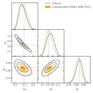
Figure 7: Validation of the $\Delta\chi^{2}<1$ scale cuts. We compare constraints from a noiseless data vector produced at the fiducial cosmology (dark blue) to those obtained from a contaminated data vector obtained by rescaling the matter power spectrum using eq. 25 with the OWLS AGN simulation, both using the fiducial model. The nested, filled regions show the , $1\sigma$ and $2\sigma$ contours, corresponding to roughly 24%, 68% and 95% confidence regions. The mean of the fiducial posterior, which is represented by the blue plus sign, lies within the contour of the contaminated posterior.

3.5.2 Alternative scale cuts ($k_{\rm max}$)

We consider a second kind of multipole cuts derived from approximate, small-scale cuts of three-dimensional Fourier modes, which is motivated by theoretical considerations. Namely, assuming that the model for the matter power spectrum is valid up to a certain wavenumber $k_{\rm max}$, we aim at discarding multipoles $\ell$ receiving significant contributions from smaller scales (i.e. for $k>k_{\rm max}$). To do so, we follow Doux et al. (2021) and rewrite eq. 22 as an integral over $k$-modes, using the change of variables $k=\ifrac{\quantity(\ell+1/2)}{\chi(z)}$. We then define the scale $k_{>\alpha}(\ell)$ at which the integral for $C_{\ell}$ reaches a fraction $\alpha<1$ of its total value, such that

$$\int_{-\infty}^{\ln k_{>\alpha}(\ell)}\differential{\ln k}{\derivative{C_{\ell}}{\ln k}}=\alpha C_{\ell}.$$ (28)

For a given choice of $\alpha$ and $k_{\rm max}$, we then obtain the small-scale multipoles cut by numerically solving for $\ell_{\rm max}$ such that ${k_{>\alpha}(\ell_{\rm max})=k_{\rm max}}$. Here, we set $\alpha=0.95$, such that scales at wavenumbers $k$ larger than $k_{>\alpha}(\ell)$ contribute 5% of the total signal. We will consider different values of $k_{\rm max}$ in the range $1\text{\,}\mathrm{\mathit{h}}\text{\,}{\mathrm{Mpc}}^{-1}5\text{\,}\mathrm{\mathit{h}}\text{\,}{\mathrm{Mpc}}^{-1}$.

Note that, in general, the validity of the model depends on redshift, as non-linearities increase at lower redshift. However, we will use the same $k_{\rm max}$ value for all ten redshift bin pairs, which in practice is limited by the low redshift bin. We show the cuts corresponding to ${k_{\rm max}=\text{$135\text{\,}\mathrm{\mathit{h}}\text{\,}{\mathrm{Mpc}}^{-1}$}}$ with dashed lines in figs. 4 and 5. These cuts leave $71156228$ data points, respectively. The highest multipole used in this work is $\ell_{\rm max}\approx 1600$ for redshift bin 4, for $k_{\rm max}=\text{$5\text{\,}\mathrm{\mathit{h}}\text{\,}{\mathrm{Mpc}}^{-1}$}$.

3.6 Sampling, parameter inference and tensions

Throughout this work, we assume a multivariate Gaussian likelihood, as detailed in section 3.3, to carry out a Bayesian analysis of our data. The theoretical calculations are performed with the CosmoSIS framework (Zuntz et al., 2015). We sample the posterior distributions using PolyChord (Handley et al., 2015), a sophisticated implementation of nested sampling, with 500 live points and a tolerance of 0.01 on the estimated evidence. We report parameter constraints through one-dimensional marginal summary statistics computed and plotted with GetDist (Lewis, 2019), as

$$\textrm{Parameter = 1D mean}_{-\textrm{lower 34\% bound}}^{+\textrm{upper 34\% bound}}\textrm{ (MAP value)},$$

where the maximum a posterior (MAP) is reported in parenthesis.

We will compute a number of metrics to characterize and interpret the inferred posterior distributions. For a number $N_{\rm param}$ of varied parameters, the number of parameters effectively constrained by the data is given by

$$N_{\rm eff}=N_{\rm param}-\Tr(\mathcal{C}_{\Pi}^{-1}\mathcal{C}_{p}),$$ (29)

where $\mathcal{C}_{\Pi}$ and $\mathcal{C}_{p}$ are the covariance matrices of the prior and posterior, approximated as Gaussian distributions, and $\Tr$ is the trace operator (Raveri & Hu, 2019). For a given posterior and its corresponding prior, we will also compute the Karhunen–Loève (KL) decomposition that measures the improvement of the posterior with respect to the prior (Raveri & Hu, 2019; Raveri et al., 2020). We can then project the observed improvement onto a set of modes, that we restrict to power laws in the cosmological parameters. Finally, we will characterize the level of disagreement between posterior distributions using the posterior shift probability, as described in Raveri & Doux (2021). This metric is based on the parameter difference distribution obtained by differenciating samples from two independent posteriors, and computing the volume with the isocontour of a null difference. To do so, we will use the tensiometer package (see previous references and Dacunha et al., 2021), which fully handles the non-Gaussian nature of the derived posteriors.

4 Validation

In this section, we present a number of tests of our analysis framework. In section 4.1, we introduce simulations that we use to verify that measured spectra are not significantly impacted by known systematic effects ($B$-modes and PSF leakage) in section 4.2, to validate the measurement pipeline and the covariance in section 4.3, and to test the accuracy of our theoretical model and its impact on cosmological parameter inferences in section 4.4.

4.1 Simulations

4.1.1 Gaussian simulations with DES Y3 data

In the following sections, we use a large number of Gaussian simulations to validate the cosmic shear power spectra measurements, obtain a covariance matrix for $B$-modes spectra and cross-spectra with the PSF ellipticities. To make them as close as possible to DES Y3 data, we use the actual positions and randomly rotated shapes of the galaxies in the DES Y3 catalog. This ensures that the masks and the noise power spectra are identical to those of the real data measurements.

The generation of a single simulation proceeds as follows. Given predictions for the shear $E$-mode spectra at the fiducial model, $C_{\ell}^{ab}$, we generate a full-sky realization of the four correlated shear fields at a resolution of $N_{\rm side}=1024$. To do so, we use the definition of the spectra, eq. 3, as the covariance of the spherical harmonic coefficients of the fields to sample four-dimensional vectors, $(E_{\ell m}^{1},E_{\ell m}^{2},E_{\ell m}^{3},E_{\ell m}^{4})$, for $0\leq\ell<3N_{\rm side}$, $-{\ell\leq m\leq+\ell}$, which are independent for different $(\ell,m)$. We then use the alm2map function of healpy (Zonca et al., 2019) in polarization mode, with $T_{\ell m}^{i}=B_{\ell m}^{i}=0$, to generate the four correlated, true (but pixelated) shear maps. The next step consists in sampling these fields. As explained above, we use the DES Y3 catalog of (mean- and response-corrected) ellipticities, to which we apply random rotations, and the positions of the galaxies as input. The random rotations are obtained by multiplying the complex ellipticities, $\mathbf{e}=e_{1}+ie_{2}$, by $e^{2i\theta}$, where $\theta$ is the random rotation angle. For a galaxy $i$ in redshift bin $a$, the ellipticity in the mock catalog is given by

$$\mathbf{e}_{i}^{\prime}=\frac{\bm{\gamma}_{i}^{a}+e^{2i\theta}\mathbf{e}_{i}}{1+e^{2i\theta}\bm{\gamma}_{i}^{a*}\mathbf{e}_{i}},$$ (30)

where $\bm{\gamma}_{i}^{a}$ is the value of the (complex) shear field corresponding to the $a$-th redshift bin at the position of galaxy $i$. This procedure is justified by the fact that the variance of the shear fields is about $10^{3}$ times smaller than the variance due to intrinsic shapes, $\sigma_{e}^{2}\sim 0.3^{2}$, such that the variance of the new ellipticities remains extremely close to that of the true ellipticities.

We then perform power spectra measurements on these mock catalogs with the same pipeline that is used on data, except that these spectra need not be corrected for the pixel window function. The mean residuals with respect to the expected ($E$-mode) power spectra computed with eq. 14 using mixing matrices are shown in the lower left panel of fig. 6 for $10\,000$ simulations, showing agreement within 5% of the error bars. We also find that the (small but non-zero) $B$-mode power spectra measured in these simulations are consistent, at the same level, with expectations from $E$-mode leakage computed using eq. 14.

Note that the real space analysis of DES Y3 lensing and clustering data (DES Collaboration, 2022) relied on log-normal simulations using Flask (Xavier et al., 2016) to partially validate the covariance, as detailed in Friedrich et al. (2021). However, those were mainly used to evaluate the effect of the survey geometry, which is already accounted for by NaMaster (Alonso et al., 2019), and need not be validated here. Therefore, we use simpler, Gaussian simulations to validate the measurement pipeline and obtain empirical covariance matrices (for $B$-mode and PSF tests). In order to validate the full covariance matrix, including the non-Gaussian contributions, we will rely on the DarkGridV1 suite of simulations (see section 4.1.2), which rely on full $N$-body simulations and are tailored for lensing studies.

4.1.2 DarkGridV1 suite of simulations

The DES Y3 analysis of the convergence peaks and power spectrum presented in Zürcher et al. (2022) relied on the DarkGridV1 suite of weak lensing simulations. They were obtained from fifty $N$-body, dark matter-only simulations produced using the PKDGrav3 code (Potter et al., 2017). Each of these consists of $768^{3}$ particles in a $900\text{\,}{\mathrm{\mathit{h}}}^{-1}\text{\,}\mathrm{Mpc}$ box, which is replicated $14^{3}$ times to reach a redshift of 3. Snapshots are assembled to produce density shells and the corresponding (true) convergence maps for the four DES Y3 redshift bins. These simulations are then populated with DES Y3 galaxies, in a way similar to what is done for Gaussian simulations (see section 4.1.1). This operation is repeated with a hundred noise realizations per simulation, thus producing $5000$ power spectra measurements.

We will use these measurements to compute an empirical covariance matrix that includes non-Gaussian contributions, and that can be compared to our analytic covariance matrix, thus providing a useful cross-check.

4.1.3 Buzzard v2.0 simulations

The Buzzard v2.0 simulations are a suite of simulated galaxy catalogs built on $N$-body simulations and designed to match important properties of DES Y3 data. These simulations were used to validate the configuration space analysis of galaxy lensing and galaxy clustering within the DES Y3 analysis and we refer the reader to DeRose et al. (2021) for greater details.

In brief, the lightcones were obtained by evolving particles initialized at redshift $z=50$ with an optimized version of the Gadget $N$-body code (Springel, 2005). The lensing fields (convergence, lensing, magnification) were computed by ray-tracing the simulations with the CalcLens code (Becker, 2013), over 160 lens planes in the redshift range ${0\leq z\leq 2.35}$, and with a resolution of $N_{\rm side}=8192$. The simulations were then populated with source galaxies so as to mimic the density, the ellipticity dispersion and photometric properties of the DES Y3 sample. The Sompz method was applied to these mock catalogs so as to divide them into four tomographic bins of approximately equal density, thus producing ensemble of redshift distributions that were validated against the known true redshift distributions (see Myles, Alarcon et al., 2021, for details).

We will use sixteen Buzzard simulations to perform an end-to-end validation of our measurement and inference pipelines in section 4.4.2. It is worth noting that these simulations do not incorporate the effects of massive neutrinos on the matter power spectrum, nor those imparted to intrinsic alignments. When analyzing these simulations, we will therefore fix the total mass of neutrinos to zero, and assume null fiducial values of the IA parameters (though they will be varied with the same flat priors).

4.2 Validation of power spectrum measurements

In this section, we study the potential contamination of the signal with two measurements. First, we verify that the $B$-mode component of the power spectra is consistent with the null hypothesis of no $B$-mode, as any cosmological or astrophysical source of $B$-mode is expected to be very small. Second, we estimate the contamination of the signal by the PSF, which, if incorrectly modeled, would leak into the estimated cosmic shear $E$-mode spectra, and therefore bias cosmology.

4.2.1 $B$-modes

As mentioned in section 3.1, gravitational lensing does not produce $B$-modes, to first order in the shear field and under the Born approximation, i.e. when the signal is integrated along the line of sight instead of following distorted photon trajectories. Second- and higher-order effects as well as source clustering and intrinsic alignments are expected to produce non-zero, but very small $B$-modes. However, the contamination of the ellipticities by various systematic effects, first and foremost by errors in the PSF model, are expected to produce much larger $B$-modes in practice. Indeed, the PSF does not possess the same symmetries as cosmological lensing, and its $E$- and $B$-mode spectra are almost identical. Therefore, any leakage due to a mis-estimation of the PSF could induce $B$-modes in galaxy ellipticities. As a consequence, measuring $B$-modes in the estimated shear maps and verifying that they are consistent with a non-detection (or pure shape-noise) constitutes a non-sufficient but nevertheless useful test of systematic effects (Becker & Rozo, 2016; Asgari et al., 2017; Asgari & Heymans, 2019; Asgari et al., 2019).

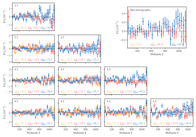
Figure 8: $EB$ and $BB$ cosmic shear power spectra measured with DES Y3 data for each pair of tomographic bins in the lower triangle, and the entire sample in the upper right panel (note that the $EB$ and $BE$ power spectra are different only for cross-redshift bin spectra). Error bars are computed from $10\,000$ Gaussian simulations using the DES Y3 catalog ellipticities and positions, as explained in section 4.1.1. We find a $\chi^{2}$ of $344.0$ for 320 degrees of freedom for tomographic $B$-mode power spectra, corresponding to a probability-to-exceed of 0.17. We find a $\chi^{2}$ of $535.4$ for 512 degrees of freedom for $EB$ tomographic cross-power spectra (counting all 16 independent bin pairs), corresponding to a probability-to-exceed of 0.23. Individual $\chi^{2}$ are reported for each redshift bin pairs in the corresponding panels. In the non-tomographic case, we find, for the $B$-mode power spectrum, a $\chi^{2}$ of $40.0$ for 32 degrees of freedom, corresponding to a probability-to-exceed of 0.16.

Figure 8 shows measurements of the tomographic $B$-mode power spectra in blue for DES Y3 data. We use $10\,000$ Gaussian simulations presented in section 4.1.1 to compute the covariance matrix (we have verified convergence) and obtain a total $\chi^{2}$, for the stacked data vector of $B$-mode spectra, of $344.0$ for 320 degrees of freedom, corresponding to a probability-to-exceed of 0.17. This is consistent with the null hypothesis of no $B$-modes. In addition, we show $EB$ cross-spectra in fig. 8 for completeness, finding a $\chi^{2}$ of $535.4$ for 512 degrees of freedom, and a probability-to-exceed of 0.23. We also show, for completeness, measurements of the non-tomographic $B$-mode power spectrum, already presented in Gatti, Sheldon et al. (2021c). In this case, we find a $\chi^{2}$ of $40.0$ for 32 degrees of freedom and a probability-to-exceed of 0.16. Note that Gatti, Sheldon et al. (2021c) also included a test where the galaxy sample was split in three bins, as a function of the PSF size at the positions of the galaxies, and found agreement with the hypothesis of no $B$-mode.

4.2.2 Point spread function

Jarvis et al. (2021) introduced the new software Piff to model the point spread function (PSF) of DES Y3 data, using interpolation in sky coordinates with improved astrometric solutions. Although the impact of the PSF on DES Y3 shapes and real-space shear two-point functions was already investigated in Gatti, Sheldon et al. (2021c) and Amon et al. (2022), we investigate PSF contamination in harmonic space as the leakage of PSF residuals might differ from those in real space. We do so by measuring $\rho$-statistics (Rowe, 2010) in harmonic space and estimate the potential level of contamination of the data vector.

Our detailed results are presented in appendix A. We conclude that we find no significant contamination and that the residual contamination has negligible impact on cosmological constraints.

4.3 Validation of the covariance matrix

We compare the fiducial covariance matrix to the covariances estimated from Gaussian simulations described in section 4.1.1 as well as the DarkGridV1 simulations described in section 4.1.2.

The middle left panel of fig. 6 shows the ratios of the square-root of the diagonals of those covariance matrices. When compared to the covariance estimated from Gaussian simulations, we find excellent agreement, at the 5% level across all scales and redshift bin pairs. Our fiducial, semi-analytical covariance predicts only slightly larger error bars, at the $23$% level. We also find very good agreement with the covariance matrix computed from DarkGridV1 simulations, with the fiducial covariance matrix showing smaller error bars, at the 15% level, for the largest scales only. For both sets of simulations, we also compared diagonals of the off-diagonal blocks (i.e. the terms $\operatorname{cov}(C_{\ell}^{ab},C_{\ell^{\prime}}^{cd})$ with $ab\neq cd$ but $\ell=\ell^{\prime}$) and found good agreement, up to the uncertainty due to the finite number of simulations. Finally, we verified that replacing the analytic covariance matrix by the DarkGridV1 covariance matrix has negligible impact on cosmological constraints inferred from the fiducial data vector (shifts below $0.1\sigma$), as shown in section C.1.

4.4 Validation of the robustness of the models

In this section, we demonstrate the robustness of our modeling using synthetic data in section 4.4.1, and using Buzzard simulations in section 4.4.2.

4.4.1 Validation with synthetic data

Our fiducial scale cuts, as explained in section 3.5.1, are constructed in such a way as to minimize the impact on cosmology from uncertainties in the small-scale matter power spectrum due to baryonic feedback, as shown in fig. 7.

We further test the robustness of our fiducial model, based on HaloFit, by testing other prescriptions for the non-linear matter power spectrum. To do so, we compare constraints, inferred with the same model, but for different synthetic data vectors computed 1. with HaloFit, 2. with HMCode with dark matter only (i.e. using $A_{\rm HM}=3.13$), and 3. with the Euclid Emulator (Euclid Collaboration et al., 2019). These data vectors are compared in fig. 5 and the constraints are shown in fig. 20, which shows that contours are shifted by less than in the $(S_{8},\Omega_{\rm m})$ plane.

We also aim at constraining the effect of baryonic feedback using alternative scale cuts based on a $k_{\rm max}$ cut-off in Fourier space, as explained in section 3.5.2. In order to validate the robustness of this alternative model, we follow a similar approach and consider predictions for the shear power spectra from four hydrodynamical simulations (Illustris, OWLS AGN, Horizon AGN and MassiveBlack II), as shown in fig. 5. We then build corresponding data vectors using HaloFit and a rescaling of the matter power spectrum, as in eq. 25. Next, we analyze those data vectors using 1. the true model considered here (i.e. HaloFit and rescaling), and then 2. HMCodewith one free parameter. We finally test whether the $(S_{8},\Omega_{\rm m})$ best-fit parameters for the true model are within the contours of the posterior assuming HMCode.

When varying only $A_{\rm HM}$, we do find that this test passes for $k_{\rm max}=\text{$135\text{\,}\mathrm{\mathit{h}}\text{\,}{\mathrm{Mpc}}^{-1}$}$ with biases of at most (and typically ), even though the inferred $A_{\rm HM}$ parameter largely varies across simulations (we find posterior means of $2.22.73.43.6$ for Illustris, OWLS AGN, Horizon AGN and MassiveBlack II, respectively). This means that biases introduced by HMCode, if any, are not worse than potential projection effects found when using the true model, all of which are found to be below the level of .

4.4.2 Validation with Buzzard simulations

In this section, we use Buzzard simulations (see section 4.1.3) to validate our measurement and analysis pipelines together. Precisely, we verify that 1. we are able to recover the true cosmology used when generating Buzzard simulations and 2. the model yields a reasonable fit to the measured shear spectra.

We start by measuring cosmic shear power spectra and verify that the mean measurement (not shown) is consistent with the theoretical prediction from our fiducial model at the Buzzard cosmology, using the true Buzzard redshift distributions, and with a covariance recomputed with these inputs.

We then run our inference pipeline on the mean data vector, first with the covariance corresponding to a single realization, and then with a covariance rescaled by a factor of $1/16$, to reflect the uncertainty on the average of the measurements. The first case is testing whether we can recover the true cosmology on average, while the second is a stringent test of the accuracy of the model, given that error bars are divided by $\sqrt{16}=4$ with respect to observations with the DES Y3 statistical power. For these tests, the priors on shear and redshift biases are centered at zero, with a standard deviation of 0.005.

The 68% and 95% confidence contours are shown in fig. 9 for both covariances, using the fiducial $\chi^{2}<1$ scale cuts. We only show the contours for the best constrained parameters ($\Omega_{\rm m}$, $\sigma_{8}$ and $S_{8}$) but we verified that the true cosmology is recovered in the full parameter space. We find that it is perfectly recovered in the first case and within $1\sigma$ contours in the second case, consistent with fluctuations on the mean Buzzard data vector. We find that the effective number of constrained parameters is $N_{\rm eff}\approx$7.8$$ in the first case, whereas, in the second case, we find $N_{\rm eff}\approx$9.6$$ (recall we fix the neutrino mass to zero for tests on Buzzard, so $N_{\rm param}=18$ here). In the second test, we find that $\chi^{2}=139.4$ at the best-fit parameters (maximum a posteriori) for $N=119$ data points, and $N-N_{\rm eff}$ degrees of freedom, such that the best-fit $\chi^{2}$ corresponds to a probability-to-exceed of $2.7$%. For $k_{\rm max}$ cuts, we also recover the input cosmology within error bars and find $\chi^{2}/(N-N_{\rm eff})$ of $98.4/61.7$, $191.6/146.1$ and $254.5/217.8$ respectively for $k_{\rm max}$ of $135\text{\,}\mathrm{\mathit{h}}\text{\,}{\mathrm{Mpc}}^{-1}$ (although note we will not use this combination of model and scale cuts on data). Together, these tests suggest that the accuracy of our fiducial model exceeds that required by the statistical power of DES Y3 data.

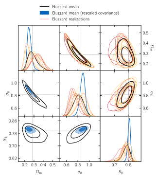
Figure 9: Validation of the analysis framework with Buzzard simulations. We show the one- and two-dimensional marginal posterior distributions corresponding to the mean Buzzard data vector with the data covariance (black) and the same covariance rescaled by a factor $1/16$ (blue). The posteriors obtained for each realization are shown in yellow to red.

We then run our inference pipeline on each realization to visualize the scatter in the posteriors due to statistical fluctuations. This exercise allows us to verify that the model does not feature catastrophic degeneracies that have the potential to bias the marginal posterior distributions over cosmological parameters, in particular in the $(S_{8},\Omega_{\rm m})$ plane. The contours are shown in fig. 9, along with the contours obtained from the mean Buzzard data vector. We also compute the $\chi^{2}$ at best fit for each realization and find that the distribution is perfectly consistent with a $\chi^{2}$ distribution with $N-N_{\rm eff}$ degrees of freedom, where we find $N_{\rm eff}\approx$7.8\pm 0.2$$ in these cases.

5 Blinding

We follow a blinding procedure, decided beforehand, that is meant to prevent confirmation and observer biases, as well as fine tuning of analysis choices based on cosmological information from the data itself. After performing sanity checks of our measurement and modeling pipelines that only drew from the data basic properties such as its footprint and noise properties, we proceeded to unblind our results in three successive stages as described below. It is worth noting, though, that as this work follows the real space analysis of Amon et al. (2022); Secco, Samuroff et al. (2022), the blinding procedure is meant to validate the components of the analysis that are different, such as the cosmic shear power spectrum measurements, the scale cuts, and the covariance matrix.

Stage 1. The shape catalog was blinded by a random rescaling of the measured conformal shears of galaxies, as detailed in Gatti, Sheldon et al. (2021c). This step preserves the statistical properties of systematic tests while shifting the inferred cosmology. A number of null tests were presented in Gatti, Sheldon et al. (2021c) to test for potential additive and multiplicative biases before deeming the catalog as science-ready and unblinding it. In the previous section section 4.2, we repeated two of these tests in harmonic space, namely the test of the presence of $B$-modes and the test of the contamination by the PSF.

Once all these tests had passed, we used the unblinded catalog to measure the shape noise power spectrum and compute the Gaussian contribution to the covariance matrix. We then repeated the systematic and validation tests, in particular those based on Gaussian simulations where shape noise is inferred from the data.

Stage 2. Using the updated covariance matrix, we proceeded to validate analysis choices with synthetic data. We first determined fiducial scale cuts based on the requirement that baryonic feedback effects do not bias cosmology at a level greater than , as detailed in section 3.5.1. We then verified that baryonic effects as predicted from a range of hydrodynamical simulations do not bias cosmology for alternative scale cuts, provided that HMCode (with a free baryonic amplitude parameter) is used instead of HaloFit, as detailed in section 4.4.1. Finally, we verified that effects that are not accounted for in the model do not bias cosmology, e.g. PSF residual contamination in appendix A, and higher-order lensing effects and uncertainties in the matter power spectrum using the $N$-body Buzzard simulations section 4.4.2.

Stage 3. Before unblinding the data vector and cosmological constraints, we performed a last series of sanity checks. In particular, we verified that the model is a good fit to the data by asserting that the $\chi^{2}$ statistic at the best-fit parameters corresponds to a probability-to-exceed above 1%. We found that the best-fit $\chi^{2}$ is 129.3 for 119 data points and $N_{\rm eff}\approx 5.6$ constrained parameters, corresponding to a probability-to-exceed of 14.6%. We also verified that the marginal posteriors of nuisance parameters were consistent with their priors. Finally, we performed two sets of internal consistency tests, in parameter space and in data space. For the tests in parameter space, we compared, with blinded axes, constraints for $(S_{8},\Omega_{\rm m})$ from the fiducial data vector with constraints from subsets of the data vector, first removing one redshift bin at a time, and then removing large or small angular scales, as detailed in items a and b of section C.1. The tests in data space, presented in section C.2, are based on the posterior predictive distribution (PPD), and follow the methodology presented in Doux et al. (2020). The PPD goodness-of-fit test yields a calibrated probability-to-exceed of 11.6%. These tests are detailed in appendix C, along with other post-unblinding internal consistency tests.

After this series of tests all passed, we plotted the data and compared it to the best-fit model, as shown in fig. 4, and finally unblinded the cosmological constraints, presented in the next section.

6 Cosmological constraints

This section presents our main results. We use measurements of cosmic shear power spectra from DES Y3 data to constrain the $\Lambda$CDM model in section 6.1. We then explore alternative analysis choices to constrain intrinsic alignments in section 6.2 and baryonic feedback in section 6.3. We compare our results to other weak lensing analyses of DES Y3 data in section 6.4, namely the comic shear two-point functions (Amon et al., 2022; Secco, Samuroff et al., 2022), convergence peaks and power spectra (Zürcher et al., 2022) and convergence second- and third-order moments (Gatti et al., 2021b), and to weak lensing analyses from the KiDS and HSC collaborations in section 6.5. Finally, as an illustrative exercise, we reconstruct the matter power spectrum from DES Y3 cosmic shear power spectra using the method of Tegmark & Zaldarriaga (2002) in section 6.6. A number of internal consistency tests are also presented in appendix C and the full posterior distribution is shown in appendix D.

Note that, for all the constraints that are presented in the following sections, we have recomputed the effective number of constrained parameters and verified that the $\chi^{2}$ statistic at best fit corresponds to a probability-to-exceed above 1%.

6.1 Constraints on $\Lambda$CDM

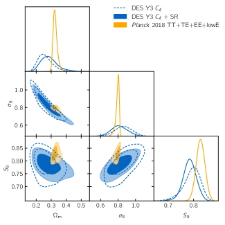
Figure 10: Cosmological constraints on the amplitude of structure $\sigma_{8}$, the total matter density $\Omega_{\rm m}$ and their combination ${S_{8}\equiv\sigma_{8}\sqrt{\Omega_{\rm m}/0.3}}$. The inner (outer) contours show 68% (95%) confidence regions. Constraints from DES Y3 cosmic shear power spectra with the two sets of fiducial scale cuts are shown in blue, with (solid) and without (dashed) shear ratios (Sánchez, Prat et al., 2021). Constraints obtained from Planck 2018 measurements of cosmic microwave background temperature and polarization anisotropies are shown in yellow (Planck Collaboration et al., 2020).

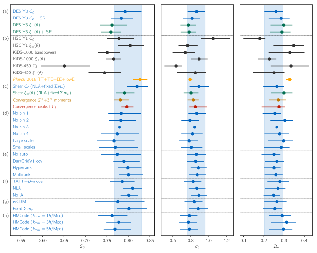
Figure 11: Comparison of one-dimensional marginal posterior distributions over the parameters $S_{8}\equiv\sigma_{8}(\Omega_{\rm m}/0.3)^{0.5}$, $\sigma_{8}$ and $\Omega_{\rm m}$, from DES Y3 data as well as other experiments, and consistency tests for this work (in blue). (a) Constraints obtained from the harmonic (this work) and real (Amon et al., 2022; Secco, Samuroff et al., 2022) space analyses of DES Y3 data are shown in blue and green (see also fig. 14), both with and without shear ratio information (SR, Sánchez, Prat et al., 2021). (b) Constraints from other weak lensing surveys, namely HSC Y1 (Hikage et al., 2019; Hamana et al., 2020), KiDS-1000 (Asgari et al., 2021) and KiDS-450 (Hildebrandt et al., 2017; Köhlinger et al., 2017) are shown in gray, and constraints from cosmic microwave background observations from Planck 2018 are shown in yellow (Planck Collaboration et al., 2020). (c) Constraints from four weak lensing analyses of DES Y3 data are compared, including the analysis of mass map moments (Gatti et al., 2021b) and peaks (Zürcher et al., 2022), and illustrating a high level of consistency (see also fig. 15). (d) Consistency tests where redshift bins are removed one at a time (first four) and where the data vector is split into its large- and small-scale data points (last two) (see also appendix C). (e) Various other consistency tests: removing auto power spectra, swapping the covariance matrix, and marginalizing over redshift distribution uncertainties with HyperRank and MultiRank (see also appendix C). (f) Modeling robustness test for intrinsic alignment (IA), including $B$-mode power spectra, or replacing TATT by NLA, or removing IA contributions altogether (see also section 6.2 fig. 12). (g) Other robustness test, freeing the dark energy equation-of-state $w$ or fixing the neutrino mass to $0.06\text{\,}\mathrm{eV}$. (h) Baryonic feedback tests where the matter power spectrum is computed with HMCode instead of HaloFit, and fiducial scale cuts are replaced with $k_{\rm max}=\text{$135\text{\,}\mathrm{\mathit{h}}\text{\,}{\mathrm{Mpc}}^{-1}$}$ scale cuts (see also section 6.3 and fig. 13).

We present here our constraints on $\Lambda$CDM assuming the fiducial model presented in section 3.2, that is, using HaloFit for the matter power spectrum and TATT for intrinsic alignments. Constraints are shown in blue in fig. 10 and compared to constraints from Planck 2018 measurements of cosmic microwave background temperature and polarization anisotropies (Planck 2018 TT+TE+EE+lowE, Planck Collaboration et al., 2020), in yellow. The one-dimensional marginal constraints are also shown in fig. 11 along with constraints for all variations of the analysis, and the full posterior is shown in fig. 25. Using only shear power spectra (i.e. no shear ratio information), we find

$$\Omega_{\rm m} =0.260^{+0.035}_{-0.057}\;(0.242), C_{\ell}$$ [ TATT]

$$\sigma_{8} =0.863\pm 0.096\;(0.902), C_{\ell}$$ [ TATT]

$$S_{8} =0.793^{+0.038}_{-0.025}\;(0.810), C_{\ell}$$ [ TATT]

where we report the mean, the 68% confidence intervals of the posterior, and the best-fit parameter values, i.e. the mode of the posterior, in parenthesis. The corresponding theoretical shear power spectra are shown in fig. 4, showing good agreement with data, consistent with the $\chi^{2}$ at best-fit of 129.3. The best constrained combination of parameters ${\sigma_{8}\quantity(\Omega_{\rm m}/0.3)^{\alpha}}$, inferred from a principal component analysis, is given by

$$\sigma_{8}\quantity(\Omega_{\rm m}/0.3)^{0.595} =0.781\pm 0.032\;(0.794). C_{\ell}$$ [ TATT]

We also compute the Karhunen–Loève (KL) decomposition to quantify the improvement of the posterior with respect to the prior using tensiometer (see section 3.6). We find that the KL mode that is best constrained by the data corresponds to ${\alpha={0.521}}$, which is remarkably close to the $S_{8}$ ($\alpha=0.5$) parameter theoretically inferred in Jain & Seljak (1997). A visualization of the KL decomposition is also given in appendix D.

We then include shear ratio information (Sánchez, Prat et al., 2021) to further reduce the uncertainty on $S_{8}$, as shown by the filled contours in fig. 10. We find this addition improves constraints on $S_{8}$ by about 18% and yields a more symmetric marginal posterior, with

$$S_{8} =0.784\pm 0.026\;(0.798), C_{\ell}$$ [+SR TATT]

$$\sigma_{8}\quantity(\Omega_{\rm m}/0.3)^{0.598} =0.783\pm 0.021\;(0.788). C_{\ell}$$ [+SR TATT]

This additional data noticeably removes part of the lower tail in $S_{8}$, which is due to a degeneracy with IA parameters, as will be seen in section 6.2, and also improves constraints on redshift distributions uncertainties by 10-30%. The volume of the two-dimensional marginal $(S_{8},\Omega_{\rm m})$ posterior, as approximated from the sample covariance, is reduced by about 20% when including shear ratios.

In comparison to constraints from Planck 2018, we find a lower amplitude of structure $S_{8}$. We estimate the tension with the parameter shift probability metric using the tensiometer package, which accounts for the non-Gaussianity of the posterior distributions (Raveri & Doux, 2021), and find tensions of about and with and without shear ratios, respectively.

Finally, we note that DES Y3 shear data alone is not able to constrain the dark energy equation-of-state $w$. We find that the evidence ratio between $w$CDM and $\Lambda$CDM is $R_{w/\Lambda}=$0.68\pm 0.18$$, which is inconclusive, based on the Jeffreys scale. We thus find no evidence of a departure from $\Lambda$CDM, consistent with Amon et al. (2022) and Secco, Samuroff et al. (2022).

6.2 Constraints on intrinsic alignments

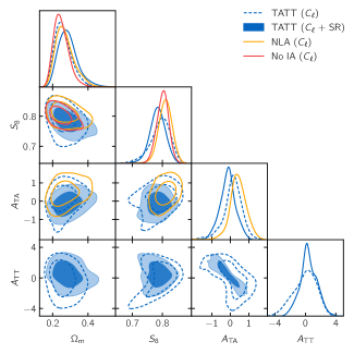
Figure 12: Constraints on cosmological and intrinsic alignment (IA) parameters from DES Y3 cosmic shear power spectra. The three colors refer to the assumed IA model: TATT in blue, NLA in orange and no IA in red. The filled blue contours include information from shear ratios while the dashed ones do not. Shear ratios are not included for the NLA and no IA models.

In this section, we focus on constraints on intrinsic alignments (IA) and explore the robustness of cosmological constraints with respect to the IA model.

The fiducial model, TATT, accounts for the possibility of tidal torquing and has five free parameters in the DES Y3 implementation (see table 1). Figure 12 shows constraints on the amplitude parameters for the tidal alignment and tidal torquing components. As stated in Blazek et al. (2019), the II component of the TATT model, which is found to dominate over the GI and IG components (see fig. 16 of Secco, Samuroff et al., 2022), receives contributions that are proportional to $A_{\rm TA}^{2}$, $A_{\rm TT}^{2}$ and $A_{\rm TA}A_{\rm TT}$. There is therefore a partial sign degeneracy between those parameters, which can be observed in the corresponding panel of fig. 12. We then find that including shear ratios significantly reduces the marginal $(A_{\rm TA},A_{\rm TT})$ posterior volume by a factor of about 3, which in turn improves cosmological constraints, as reported in the previous section. In this case, we obtain

$$A_{\rm TA} =-0.14\pm 0.43\;(-0.398), C_{\ell}$$ [+SR TATT]

$$A_{\rm TT} =0.4\pm 1.1\;(1.714). C_{\ell}$$ [+SR TATT]

These constraints alone do not exclude zero, potentially due to the aforementioned sign degeneracy. If we restrict the prior to $A_{\rm TA}>0$, we find ${A_{\rm TA}=0.30^{+0.12}_{-0.30}}$ and ${A_{\rm TT}=-0.69^{+0.83}_{-0.43}}$, with essentially unchanged cosmological constraints. We do not show constraints on the redshift tilt parameters $\alpha_{\rm TA}$ and $\alpha_{\rm TT}$, which are unconstrained by the data (which might be due to amplitude parameters being consistent with zero).

We also report constraints on the NLA model in fig. 12, a subset of TATT where $A_{\rm TT}=b_{\rm TA}=0$, which is not excluded by the data. We exclude shear ratio information here, so as to compare constraints obtained with shear power spectra alone (TATT constraints are shown by dashed lines in fig. 12). Because of the complex degeneracy between $S_{8}$ and $A_{\rm TT}$, visible in fig. 12, fixing the tidal torquing component to zero results in cosmological constraints that are improved by about 27% on $S_{8}$, and which are found to be consistent with the TATT case. Assuming the NLA model, we find

$$S_{8} =0.810\pm 0.023\;(0.834), C_{\ell}$$ [ NLA]

$$A_{\rm TA} =0.40\pm 0.51\;(0.701), \text{[$C_{\ell}$ NLA]},$$

i.e. a slightly larger value of $S_{8}$, albeit within uncertainties of the fiducial model. Finally, we note that removing IA contributions altogether further improves the constraint on $S_{8}$ by about 16%, yielding

$$S_{8} =0.801^{+0.021}_{-0.018}\;(0.836), \text{[$C_{\ell}$ no IA]},$$

also consistent with the NLA and TATT cases.

In terms of model selection, we find that going from no IA to NLA, and then from NLA to TATT improves fits by ${\Delta\chi^{2}=-0.3}$ and ${\Delta\chi^{2}=-1.1}$ respectively, while introducing two and three more parameters. The evidence ratios are given by ${R_{{\rm NLA}/{\rm TATT}}=$3.59\pm 0.93$}$, ${R_{{\rm noIA}/{\rm TATT}}=$17.5\pm 4.3$}$ and ${R_{{\rm noIA}/{\rm NLA}}=$4.88\pm 0.11$}$, marking a weak preference for NLA over TATT, but a substantial preference for no IA over TATT, according to the Jeffreys scale.

Cosmic shear analyses in harmonic space usually only exploit the $E$-mode part of the power spectrum. However, as detailed in section 3.2.3, tidal torquing generates a small $B$-mode signal, which may at least be constrained by our $B$-mode data. We validated our analysis pipeline by checking that (i) the $E$-to-$B$-mode leakage measured in our Gaussian simulations (see section 4.1.1) is consistent with expectations from mixing matrices, (ii) we do recover correct IA parameters, with tighter constraints, for synthetic data vectors for different values of the IA parameters (including non-zero $A_{\rm TT}$). We obtain constraints that are consistent for cosmological parameters inferred without $B$-mode data. However, they seem to strongly prefer non-zero $A_{\rm TT}$, and are not consistent across redshift bins. This preference is indeed entirely supported by bin pairs $3,3$ an $3,4$, that have the highest $\chi^{2}$ with respect to no $B$-mode, as shown in fig. 8. Including $B$-mode data and freeing TATT parameters, the $\chi^{2}$ for those bins are reduced by $13.5$ and $17.4$ respectively, while all other bin pairs are unaffected ($\chi^{2}$ changed by less than 1). Indeed, we find that removing bin 3 entirely makes the preference for non-zero $A_{\rm TT}$ disappear, with very small impact on the cosmology. We obtain very similar results when including shear ratios. We conclude from this experiment that DES Y3 data is not able to constrain the contribution of tidal torquing to the TATT model efficiently, leading to the model picking up potential flukes in the $B$-mode data, which has been verified to be globally consistent with no $B$-modes. Future data will place stronger constraints on $B$-modes and its potential cosmological sources.

6.3 Constraints on baryons

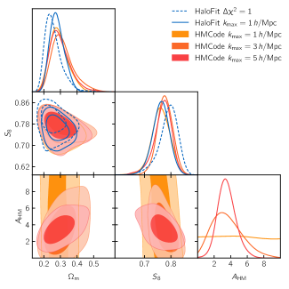
Figure 13: Constraints on cosmological and baryonic feedback parameters from DES Y3 cosmic shear power spectra. In blue, we show constraints for the fiducial model, i.e. using HaloFit. In orange to red, we show constraints using HMCode with one free parameter, while varying the $k_{\rm max}$ cut-off from 1 to  $5\text{\,}\mathrm{\mathit{h}}\text{\,}{\mathrm{Mpc}}^{-1}$ (see fig. 4). We also show, with dashed lines, the constraints for the fiducial HaloFit model and the $k_{\rm max}=$1\text{\,}\mathrm{\mathit{h}}\text{\,}{\mathrm{Mpc}}^{-1}$$ cut, which is even more conservative than our fiducial $\Delta\chi^{2}=1$ cut. Note that all constraints shown here use TATT to model intrinsic alignments and none include shear ratio information.

We now turn our attention towards baryonic feedback. Our fiducial analysis discards scales where baryonic feedback is expected to impact the shear power spectrum. However, we have shown in section 4.4.1 that HMCode provides a model that is both accurate and flexible enough for our analysis, for scale cuts with $k_{\rm max}$ in the range $1\text{\,}\mathrm{\mathit{h}}\text{\,}{\mathrm{Mpc}}^{-1}5\text{\,}\mathrm{\mathit{h}}\text{\,}{\mathrm{Mpc}}^{-1}$.

Figure 13 shows constraints obtained assuming HMCode with one free parameter, for varying scale cuts, as well as a comparison to the fiducial HaloFit model. We find cosmological constraints to be robust to the choice of $k_{\rm max}$, with deviations below . In particular, in fig. 13 we show contours for both models for $k_{\rm max}=$1\text{\,}\mathrm{\mathit{h}}\text{\,}{\mathrm{Mpc}}^{-1}$$, which is more conservative than our fiducial ${\Delta\chi^{2}=1}$ scale cut, and find very good agreement. We then find that extra data points included when raising $k_{\rm max}$ from $1\text{\,}\mathrm{\mathit{h}}\text{\,}{\mathrm{Mpc}}^{-1}5\text{\,}\mathrm{\mathit{h}}\text{\,}{\mathrm{Mpc}}^{-1}$ (71 to 228) do constrain the HMCode baryonic feedback parameter $A_{\rm HM}$, but have a relatively little impact on cosmological constraints, both in position and width. In other words, given our current error bars, cosmological information at small scales is partially lost by marginalizing over uncertainties in the baryonic feedback model. For the $k_{\rm max}=$5\text{\,}\mathrm{\mathit{h}}\text{\,}{\mathrm{Mpc}}^{-1}$$ cut, we find $\chi^{2}=235.2$ ($p=0.25$) at best-fit, and constraints given by

$$\Omega_{\rm m} =0.297^{+0.043}_{-0.071}\;(0.246), C_{\ell}$$ [ HMCode TATT]

$$S_{8} =0.769^{+0.037}_{-0.026}\;(0.762), C_{\ell}$$ [ HMCode TATT]

$$A_{\rm HM} =3.52^{+0.94}_{-1.2}\;(1.620). C_{\ell}$$ [ HMCode TATT]

This is in good agreement with cosmological constraints reported for the HaloFit model in section 6.1, although this model does favor slightly lower $S_{8}$ and $\sigma_{8}$ values, and a higher $\Omega_{\rm m}$ value, which happens to be closer to the Planck value, as seen in fig. 11. As a consequence, the tension with Planck rises to in this case. The corresponding best-fit model is represented by dashed lines in fig. 4, where we observe that, on large scales, i.e. for multipoles below the fiducial scale cuts, both models agree very well. However, on smaller scales, HMCode yields shear power spectra 10-20% lower, which, visually, seems to provide a better fit to data (again, those scales are excluded in the fiducial model).

When using HMCode with two free parameters, we find that the constraining power is entirely transferred to the second parameter, $\eta_{\rm HM}$, with very little impact on cosmological constraints. For ${k_{\rm max}=$5\text{\,}\mathrm{\mathit{h}}\text{\,}{\mathrm{Mpc}}^{-1}$}$, we find ${\eta_{\rm HM}=0.86^{+0.29}_{-0.35}}$ while $A_{\rm HM}$ is unconstrained.

The previous constraints are based on our fiducial IA model, TATT. However, we showed in the previous section that the NLA model seems favored by the data (using evidence ratios). If we use this model instead, as done in the KiDS-1000 analysis (Asgari et al., 2021), we find ${S_{8}=0.790\pm 0.024}$ and ${A_{\rm HM}=3.67^{+0.71}_{-0.92}}$, although we note immediately that we have not validated our scale cuts against this specific model and that these results should be interpreted with caution.

Our results do not allow exclusion of the dark matter only value of ${A_{\rm HM}=3.13}$ in either direction. In comparison to the hydrodynamical simulations we used in section 3.2.4 to validate the model, constraints from data are closer to Massive Black II, although the uncertainty from shear power spectra alone is too large to discriminate between baryonic feedback prescriptions. Figure 13 suggests that a better understanding of the effect of baryons on the distribution of matter will be an important task in order to be able to capture cosmological information at small scales. For the foreseeable future, this will likely require cross-correlating shear data with other probes that are sensitive to baryons, e.g. Compton-$y$ maps of the thermal Sunyaev-Zeldovich (SZ) effect with CMB maps (see, e.g., Pandey et al. 2021; Gatti et al. 2021a with DES Y3 data and Tröster et al. 2021 with KiDS-1000 data) or the kinetic SZ effect (Schaan et al., 2021; Amodeo et al., 2021). Another avenue is to exploit information from even smaller scales, e.g. using a principal component analysis to span a variety of scenarios from hydrodynamical simulations (see Huang et al. 2019 for the methodology and Huang et al. 2021 for an application to DES Y1 data) or a baryonification model (see Schneider & Teyssier 2015; Schneider et al. 2019, and Chen et al. in preparation for an application to DES Y3 data).

6.4 Consistency with other DES Y3 weak lensing analyses

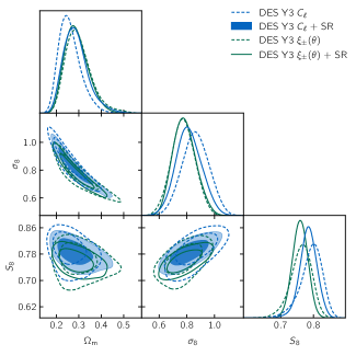
Figure 14: Comparison of cosmological constraints obtained from the analysis of cosmic shear two-point functions of DES Y3 data in real (in green, Amon et al., 2022; Secco, Samuroff et al., 2022) and harmonic space (in blue, this work). Solid contours indicate constraints that include shear ratio information Sánchez, Prat et al. (2021). We find ${\Delta S_{8}=0.025}$, with shear ratios, consistent with the expected statistical scatter ${\sigma(\Delta S_{8})\sim 0.02}$ predicted in Doux et al. (2021).

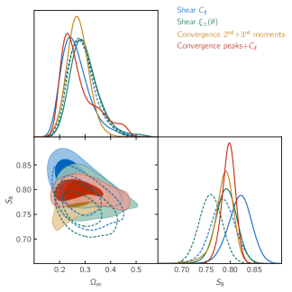
Figure 15: Comparison of cosmological constraints obtained from the analysis of DES Y3 lensing data using four different statistics: shear power spectra (this work, in blue), shear two-point functions (Amon et al., 2022; Secco, Samuroff et al., 2022, in green), convergence second and third order moments (Gatti et al., 2021b, in orange), and convergence peaks and power spectra (Zürcher et al., 2022, in red). For the first two, we have matched the modeling to that adopted for the analysis of non-Gaussian convergence statistics, namely restricting the intrinsic alignment model to NLA and fixing the total mass of neutrinos (see main text for a discussion of possible caveats). These constraints are shown by solid contours, whereas constraints obtained with the fiducial model are shown by the dashed contours, for reference. None of the constraints shown here include shear ratio information. Although the comparison requires some care, this figure highlights the overall consistency of DES Y3 lensing data and existing analyses.

In this section, we compare our results obtained from cosmic shear power spectra to other studies using DES Y3 lensing data, as detailed below. We first focus on the comparison with the real-space analysis of shear two-point functions presented in Amon et al. (2022); Secco, Samuroff et al. (2022). The study presented here is its harmonic space counterpart, in the sense that we follow a very similar methodology and use the same fiducial model. We then extend the comparison to studies that incorporate non-Gaussian information from the DES Y3 convergence (mass) map (Jeffrey, Gatti et al., 2021b), namely the analysis of peaks and power spectra from Zürcher et al. (2022), and the analysis of second and third order moments from Gatti et al. (2021b). Figures 14 and 15 show cosmological constraints obtained from those studies, which are found to be in very good agreement, illustrating the internal consistency of DES Y3 shear analyses. See also fig. 11 for a comparisom of all one-dimensional marginal constraints.

Real space two-point functions $\xi_{\pm}$. Figure 14 shows cosmological constraints obtained from two-point functions in real space (Amon et al., 2022; Secco, Samuroff et al., 2022) and in harmonic space (this work), both with and without including shear ratio information. We find that both studies yield very consistent cosmological constraints, with a preference for slightly higher $S_{8}$ from shear power spectra. However, the difference between the means of the posteriors is ${{\Delta S_{8}}=0.031}$ when excluding shear ratios, which is fairly consistent with the expected statistical scatter $\sigma(\Delta{S_{8}})\sim$0.02$$ predicted in Doux et al. (2021). The degeneracy directions are found to be slightly different, with $\alpha_{C_{\ell}}=0.595$ and $\alpha_{\xi_{\pm}}=0.552$ for harmonic and real space analyses, respectively. When including shear ratios, the difference narrows down to ${{\Delta S_{8}}=0.025}$ and the best constrained direction is almost identical, with $\alpha_{C_{\ell}}=0.598$ and $\alpha_{\xi_{\pm}}=0.586$. As a consequence of the higher value of $S_{8}$ found here, the tension with Planck is reduced from in (Amon et al., 2022; Secco, Samuroff et al., 2022) to in this work.

For IA parameters, we find an overall excellent agreement (not shown). Although the real-space analysis shows a weak preference for negative $A_{\rm TA}$ and positive $A_{\rm TT}$, we observe the same degeneracy between those parameters, with almost perfect overlap. The two parameters that describe redshift evolution are unconstrained in both cases, but the posteriors are also nearly identical. We also find that fixing the IA model to NLA results in a slightly higher value for $S_{8}$.

Non-Gaussian statistics from mass maps. Figure 15 presents cosmological constraints from all four lensing analyses. Due to difficulties in modeling non-Gaussian statistics, both analyses of moments and peaks (Gatti et al., 2021b; Zürcher et al., 2022) include IA contributions using a model based on NLA, and both fix the total mass of neutrinos to the minimum value of $0.06\text{\,}\mathrm{eV}$. In order to make the comparison more meaningful, we therefore re-analyze shear two-point functions and power spectra with these two changes, which tends to favor slightly higher values of $S_{8}$ (either change individually also goes in this direction). We warn the reader that (i) despite matching important modeling choices, there remain differences in the analysis in terms of priors, modeling pipeline technology (e.g. Zürcher et al. 2022 uses an emulator) and methodology, and (ii) the scale cuts used for two-point functions were not validated for this specific model, and should be interpreted with caution. Nevertheless, this figure illustrates the high level of consistency of these analyses – all of which followed a similar blinding procedure – and of DES Y3 lensing data.

6.5 Comparison with other lensing surveys

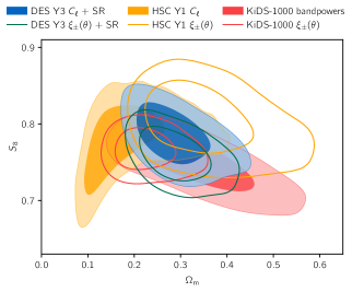
Figure 16: Comparison of cosmological constraints from the analysis of cosmic shear in harmonic (filled contours) and real space (contour lines) for DES Y3 (this work in blue, Amon et al. 2022; Secco, Samuroff et al. 2022 in green), HSC Y1 (Hikage et al., 2019; Hamana et al., 2020, in yellow) and KiDS-1000 (Asgari et al., 2021, in red). We note that these results rely on different analysis and modeling choices.

In the past two years, both the HSC and KiDS collaborations have presented cosmic shear analyses of their data in harmonic and real space. Figure 16 compares constraints obtained from DES Y3 data to those obtained from KiDS-1000 (Asgari et al., 2021) and HSC Y1 (Hikage et al., 2019; Hamana et al., 2020). Uni-dimensional marginal distributions are also shown in fig. 11. As shown in Doux et al. (2021) on simulations, statistical fluctuations are not expected to bias one estimator over the other and shift constraints in any specific direction, while unmodeled systematic effects might. We do not find any clear trend here.

Both KiDS-1000 and HSC analyses use NLA to model intrinsic alignments with fixed neutrino masses. However we decide to present constraints that were obtained from the fiducial models assumed by each collaboration for simplicity. We also note that the KiDS-1000 analysis uses a “bandpowers” estimator of shear power spectra that stems from an original measurement of two-point functions in real space with a thin spacing. A recent analysis (Loureiro et al., 2021) applying a pseudo-$C_{\ell}$ estimator found very similar constraints on $S_{8}=0.754^{+0.027}_{-0.029}$ between the bandpowers and pseudo-$C_{\ell}$ estimators, despite appreciable differences in the intrinsic alignment parameter, likely due to how the two estimator cut large-scale information. Ignoring potential correlations due to overlapping survey areas, we find our results to be in agreement at the levels with KiDS-1000 bandpowers and HSC Y1 $C_{\ell}$ analyses. Finally, we find good agreement on the IA parameter $A_{\rm TA}$ (not shown), although constraints remain broad for all three surveys.

6.6 Reconstruction of the matter power spectrum

In this section, we apply the method of Tegmark & Zaldarriaga (2002) to approximately reconstruct the linear matter power spectrum at present time, $P(k)$, from DES Y3 shear power spectra. We immediately note that this exercise is strongly model-dependent, in that it requires to assume a full cosmological model to relate shear power spectra to the matter power spectrum. Moreover, it presents subtleties in relating physical scales between the linear and non-linear power spectra, as discussed in Tegmark & Zaldarriaga (2002), and we will employ a simplified approach presented in the next paragraph. Nevertheless, assuming the Planck 2018 cosmology (Planck Collaboration et al., 2020), we may compare the power spectrum reconstructed from DES Y3 data to the expectation from Planck, which is relevant in the context of the $\sigma_{8}$ tension found in previous weak lensing surveys (Amon et al., 2022; Secco et al., 2022; Hikage et al., 2019; Hamana et al., 2020; Asgari et al., 2021), and that we also observe in fig. 10.

To do so, we recast eq. 22 as an integral over three-dimensional Fourier $k$-modes, using the change of variable ${k=(\ell+1/2)/\chi(z)}$. We then define a window matrix, W, such that the expected value of our data vector, $\expectationvalue{\hat{\mathbf{C}}_{L}}$, may be expressed as a function of the linear matter power spectrum at $z=0$, $P(k)$, computed in log-spaced $k$-bins of width $\Delta_{\ln k}$, $\mathbf{P}$, such that

$$\expectationvalue{\hat{\mathbf{C}}_{L}}\approx\textbf{{W}}\mathbf{P}.$$ (31)

This window matrix is given, for the element corresponding to $k$ and $C_{L}^{ab}$, and ignoring intrinsic alignments, by

$$\textbf{{W}}_{k,L,a,b}\approx k\Delta_{\ln k}(L+1/2)q_{a}(\chi)q_{b}(\chi)\frac{P_{\rm NL}\quantity(k,z(\chi))}{P_{\rm fid}(k)}$$ (32)

with $\chi=(L+1/2)/k$. Given the data covariance C, the reconstructed power spectrum has estimated value and covariance given by

$$\hat{\mathbf{P}} =\textbf{{S}}\textbf{{W}}^{\intercal}\textbf{{C}}^{-1}\hat{\mathbf{C}}_{L},$$ (33)

S $$=\quantity[\textbf{{W}}^{\intercal}\textbf{{C}}^{-1}\textbf{{W}}+\sigma^{-2}\textbf{{I}}]^{-1},$$ (34)

where we have included a regularization term, $\sigma$, which enables inverting eq. 31 at the price of accepting that certain $k$-modes may not be recovered from the data (the results have very low dependence on $\sigma$, if chosen large enough, in the range where the data is constraining). To ensure numerical stability, we use 20 bins in the range ${k\sim$1\text{\times}{10}^{-3}\text{\,}\mathrm{\mathit{h}}\text{\,}{\mathrm{Mpc}}^{-1}1\text{\times}{10}^{2}\text{\,}\mathrm{\mathit{h}}\text{\,}{\mathrm{Mpc}}^{-1}$}$, and subsequently rebin the estimated power spectrum within 10 bins for better visualization as well as to suppress the anticorrelation of adjacent bins. The simplification here comes from eq. 32, where the dependence on the linear matter power spectrum is made explicit by simply multiplying the numerator and denominator by $P_{\rm fid}(k)$, the power spectrum at redshift zero for the fiducial Planck 2018 cosmology. Our exercise therefore amounts to a reconstruction of the integrand over $\ln{k}$ with respect to what is expected from Planck, rather than a reconstruction of the linear matter power spectrum itself.

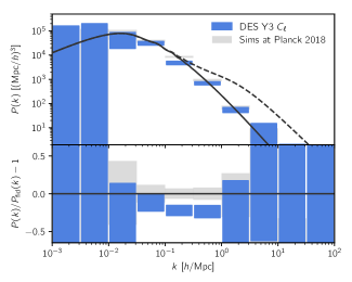
Figure 17: Matter power spectrum at redshift $z=0$ reconstructed from DES Y3 shear power spectra, using a simplified version of the method of Tegmark & Zaldarriaga (2002). The fiducial linear matter power spectrum, computed at Planck 2018 cosmology (Planck Collaboration et al., 2020), is shown by the solid, black line (the corresponding non-linear power spectrum is shown by the dashed, black line). The blue boxes, centered on ${(k,\hat{\mathbf{P}})}$ (see eq. 33) and of height given by the square-root of the diagonal of the covariance matrix S (see eq. 34), show the reconstructed power spectrum within log-spaced $k$ bins. In the background, we show in gray the result of the reconstruction for $1000$ simulated data vectors drawn from the likelihood at Planck cosmology; however, in this case, the height of the boxes represents the standard deviation of the results, offering a simple check for the covariance matrix. The reconstructed power spectrum is about 20% (or roughly ) lower than the fiducial one around $k\sim$0.3\text{\,}\mathrm{\mathit{h}}\text{\,}{\mathrm{Mpc}}^{-1}$$.

The result is shown in fig. 17. The lower panel shows the reconstructed, binned ratio of the power spectrum with respect to the prediction from Planck 2018 (in blue), compared to the results obtained from simulated DES Y3 data vectors generated by sampling the likelihood at the Planck 2018 cosmology (in gray). In the upper panel, we multiply these ratios by the fiducial linear power spectrum, shown in black. We find that the reconstructed spectrum is roughly 20% lower than the prediction in the range ${k\sim$0.03\text{\,}\mathrm{\mathit{h}}\text{\,}{\mathrm{Mpc}}^{-1}1\text{\,}\mathrm{\mathit{h}}\text{\,}{\mathrm{Mpc}}^{-1}$}$ that is constrained by DES Y3 data. In particular, the reconstruction is about low around $k\sim$0.3\text{\,}\mathrm{\mathit{h}}\text{\,}{\mathrm{Mpc}}^{-1}$$, which remains close to the linear regime.

7 Conclusions

In this work, we have used data from the first three years of observations by the Dark Energy Survey (DES Y3), including a catalog of over a hundred million galaxy shape measurements (Gatti, Sheldon et al., 2021c) split into four redshift bins (Myles, Alarcon et al., 2021), to measure tomographic cosmic shear power spectra. Our measurements over the DES Y3 footprint of $4143\text{\,}{\mathrm{deg}}^{2}$ are based on the pseudo-$C_{\ell}$ method, with a consistent spherical sky approach using the NaMaster software (Alonso et al., 2019). We generally followed the DES Y3 methodology laid out in Amon et al. (2022); Secco, Samuroff et al. (2022) and the modeling choices presented in Krause et al. (2021) to infer cosmological constraints, and found ${S_{8}\equiv\sigma_{8}\sqrt{\Omega_{\rm m}/0.3}=0.793^{+0.038}_{-0.025}\;(0.810)}$ using cosmic shear alone. We also included geometric information from small-scale galaxy-galaxy lensing ratios (Sánchez, Prat et al., 2021) to tighten the constraint to ${S_{8}=0.784\pm 0.026\;(0.798)}$.

Following Amon et al. (2022); Secco, Samuroff et al. (2022), we modeled intrinsic alignments with TATT (Blazek et al., 2019) that coherently includes tidal alignment (TA) and tidal torquing (TT) mechanisms. We found, as in Secco, Samuroff et al. (2022), that the data does not strongly favor this model over the simpler non-linear alignment (NLA) model, as the data does not seem to constrain the TT contribution efficiently (even when including $B$-modes in the analysis, which may be sourced by TT). In all cases, we find consistent cosmological constraints, although using NLA tightens constraints on $S_{8}$ by about 25%.

We include smaller scales that had been discarded in the fiducial analysis, switching from HaloFit to HMCode to model the non-linear matter power spectrum, thus including the effect of baryonic feedback, known to be a major source of uncertainty for cosmic shear at small scales (Chisari et al., 2018; Huang et al., 2019). We derived a set of scale cuts that approximately map to a cut-off $k_{\rm max}$ in Fourier modes. When raising $k_{\rm max}$ from $1\text{\,}\mathrm{\mathit{h}}\text{\,}{\mathrm{Mpc}}^{-1}$ to $5\text{\,}\mathrm{\mathit{h}}\text{\,}{\mathrm{Mpc}}^{-1}$, we found consistent cosmological constraints, while the extra statistical power appears to mainly constrain the baryonic feedback parameter, ${A_{\rm HM}=3.52^{+0.94}_{-1.2}\;(1.620)}$. This result does not rule out the dark matter-only case ($A_{\rm HM}=3.13$) nor the predictions from the hydrodynamical simulations we considered in this work. Given current error bars and theoretical uncertainties, it therefore remains difficult to extract small-scale cosmological information that is present in our cosmic shear data, thus highlighting the need to better understand the effect of baryonic processes on the clustering of matter, especially for future surveys (see, e.g. Martinelli et al., 2021).

This analysis complements other weak lensing analyses of DES Y3 data, namely the analysis of cosmic shear two-point correlation functions presented in Amon et al. (2022); Secco, Samuroff et al. (2022), convergence second- and third-order moments (Gatti et al., 2021b), and convergence peaks and power spectra (Zürcher et al., 2022), the latter two being based on maps from Jeffrey, Gatti et al. (2021b). With respect to the real-space two-point functions, we find very similar constraints, with a value of $S_{8}$ slightly higher by ${{\Delta S_{8}}=0.025}$ when including shear ratios, perfectly consistent with statistical fluctuations of order $\sigma(\Delta{S_{8}})\sim$0.02$$ predicted in Doux et al. (2021). The comparison of constraints from Gaussian and non-Gaussian statistics delivers an overall coherent picture, highlighting the cosmological information beyond two-point measurements and pointing towards the modeling improvements required for future analyses. This analysis thus provides an important consistency check of DES Y3 lensing data. It also demonstrates the feasibility of conducting a harmonic space analysis over a wide survey footprint, which could be combined with other estimators, such as the real-space correlation functions, into a joint analysis in the future. To do so, one would need to compute an accurate estimate of the cross-covariance of the different statistics considered, or to perform a simulation-based, likelihood-free analysis (see, e.g. Jeffrey et al., 2021a).

At last, we compared our results to those obtained by other weak lensing studies from the Hyper Suprime-Cam and Kilo-Degree Survey collaborations and found consistent constraints on cosmology. We also compared our results to constraints from observations of the cosmic microwave background. We found that the tension with Planck 2018 in $S_{8}$, computed with the parameter shift probability (Raveri et al., 2020; Raveri & Doux, 2021), is in this work, whereas it is in Amon et al. (2022); Secco, Samuroff et al. (2022). This shift is reflected in the inferred linear matter power spectrum, in excess by about 20% in the range ${k\sim$3\text{\times}{10}^{-2}\text{\,}\mathrm{\mathit{h}}\text{\,}{\mathrm{Mpc}}^{-1}1\text{\,}\mathrm{\mathit{h}}\text{\,}{\mathrm{Mpc}}^{-1}$}$ for Planck with respect to DES Y3. Future observations, such as the complete data from the six-year program of the DES and data from the next generation of surveys including LSST, Euclid and Roman, as well as methodological improvements will be necessary to determine whether this apparent tension is the sign of an incorrect treatment of systematic effects, or of new physics.

Data availability

A general description of DES data releases is available on the survey website at https://www.darkenergysurvey.org/the-des-project/data-access/. DES Y3 cosmological data has been partially released on the DES Data Management website hosted by the National Center for Supercomputing Applications at https://des.ncsa.illinois.edu/releases/y3a2. This includes Gold products, PSF modelling, Balrog catalogs, Deep Fields data and the Y3 galaxy catalogs, including the redshift distributions used in this analysis. The CosmoSIS software (Zuntz et al., 2015) is available at https://bitbucket.org/joezuntz/cosmosis/wiki/Home. The measurement code, used in this analysis to interface DES catalogs and NaMaster, can be obtained upon request to the corresponding author.

Appendix A Point spread function

This section presents the results of our tests for potential contamination of shear power spectra from the point spread function (PSF) and complements those presented in Jarvis et al. (2021); Gatti, Sheldon et al. (2021c).

We specifically focus on the additive biases due to PSF misestimation using $\rho$-statistics (Rowe, 2010) following the same diagnostics as Gatti, Sheldon et al. (2021c). We expect other contributions like the brighter-fatter effect, dependencies of the PSF model residuals on star and galaxy colors, and tangential shear around stars to be negligible, as discussed in Section 5 of Gatti, Sheldon et al. (2021c).

The estimated shear $\bm{\gamma^{\text{est}}}$ is decomposed as

$$\bm{\gamma^{\text{est}}}=\bm{\gamma}+\delta\bm{e}_{\text{PSF}}+\delta\bm{e}_{\text{noise}}$$ (35)

where $\bm{\gamma}$ represents the true shear, $\delta\bm{e}_{\text{noise}}$ denotes noise, and $\delta\bm{e}_{\text{PSF}}$ characterizes additive biases from PSF modeling errors. DES Y3 uses a sample of reserved stars that were not used to obtain the PSF model, and for which we can compare the modeled PSF ellipticity $\bm{e}_{\text{model}}$ to the measured ellipticity $\bm{e}_{*}$ (and similarly for PSF sizes, with $T_{\text{model}}$ and $T_{*}$). The PSF bias term can be further modeled as

$$\delta\bm{e}_{\text{PSF}}=\alpha\bm{p}+\beta\bm{q}+\eta\bm{w},$$ (36)

where $\bm{p}\equiv\bm{e}_{\text{model}}$, $\bm{q}\equiv\bm{e}_{\text{*}}-\bm{e}_{\text{model}}$, and $\bm{w}\equiv\bm{e}_{\text{*}}(T_{*}-T_{\text{model}})/T_{*}$. Under the assumption that the true shear signal $\bm{\gamma}$ does not correlate with modeling errors, the cross power spectra of galaxy shear and the PSF parameters $\bm{p}$, $\bm{q}$, and $\bm{w}$ read

$$\mathbf{C}_{\ell}\quantity(\bm{\gamma^{\text{est}}},\bm{p}) =\alpha\mathbf{C}_{\ell}\quantity(\bm{p},\bm{p})+\beta\mathbf{C}_{\ell}\quantity(\bm{q},\bm{p})+\eta\mathbf{C}_{\ell}\quantity(\bm{w},\bm{p}),$$ (37)

$$\mathbf{C}_{\ell}\quantity(\bm{\gamma^{\text{est}}},\bm{q}) =\alpha\mathbf{C}_{\ell}\quantity(\bm{p},\bm{q})+\beta\mathbf{C}_{\ell}\quantity(\bm{q},\bm{q})+\eta\mathbf{C}_{\ell}\quantity(\bm{w},\bm{q}),$$ (38)

$$\mathbf{C}_{\ell}\quantity(\bm{\gamma^{\text{est}}},\bm{w}) =\alpha\mathbf{C}_{\ell}\quantity(\bm{p},\bm{w})+\beta\mathbf{C}_{\ell}\quantity(\bm{q},\bm{w})+\eta\mathbf{C}_{\ell}\quantity(\bm{w},\bm{w}).$$ (39)

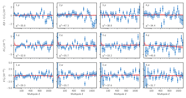
Figure 18: Cross-power spectra between galaxy shapes in the four redshift bins (from left to right) with PSF parameters $\bm{p}$, $\bm{q}$ and $\bm{w}$ (from top to bottom). The measurements are shown in blue, with error bars computed from $18\,000$ Gaussian simulations using the DES Y3 catalog ellipticities and positions, as explained in section 4.1.1. The model from eqs. 37, 38 and 39 at best-fit is shown by the red line, while the band shows the uncertainty. We find $\chi^{2}$ statistics with respect to the best fit between $29.3$ and $45.8$ ($29.3$ to $47.3$ for the null hypothesis) for 32 degrees of freedom, shown in the lower left corner for each panel, corresponding to a minimum probability-to-exceed of 0.04.

We first measured the cross power spectra of the shear and the PSF parameters $\bm{p}$, $\bm{q}$, and $\bm{w}$. We then repeated these measurements using 18,000 Gaussian simulations, as described in section 4.1.1, to obtain their covariance matrix. To calculate the cross power spectra between the PSF parameters (right-hand side of eqs. 37, 38 and 39), we split the catalog into two halves that we cross-correlate, which effectively cancels out the shot noise. We then find the best-fit scalar parameters $\alpha$, $\beta$, $\eta$ over all scales and three cross-spectra types for each tomographic redshift bin using Markov chain Monte-Carlo (MCMC) samples generated with the public software package emcee (Foreman-Mackey et al., 2013). This approach is adapted from the measurements performed in the real space analysis (Amon et al., 2022) using the same tomographic split, and the non-tomographic measurement from Jarvis et al. (2021).

	Bin 1	Bin 2	Bin 3	Bin 4
$\alpha$	$0.003_{-0.007}^{+0.007}$	$0.014_{-0.008}^{+0.008}$	$0.008_{-0.010}^{+0.010}$	$0.012_{-0.011}^{+0.011}$
$\beta$	$0.02_{-0.36}^{+0.36}$	$-0.07_{-0.38}^{+0.38}$	$0.16_{-0.38}^{+0.39}$	$-0.74_{-0.47}^{+0.46}$
$\eta$	$-5.4_{-4.4}^{+4.3}$	$0.4_{-4.8}^{+4.8}$	$1.6_{-5.0}^{+5.1}$	$-5.4_{-5.8}^{+5.9}$
$\chi^{2}$	$99.5$	$116.3$	$113.4$	$117.3$

Table 2: Values of the parameters $\alpha$, $\beta$ and $\eta$ for each redshift bin, estimated from fits to the cross-power spectra of galaxy and PSF shapes, according to equations 37, 38, 39 as well as the goodness-of-fit, $\chi^{2}$, for ${96-3}$ degrees of freedom.

We present the best-fit $\alpha$, $\beta$, $\eta$ values in Table 2. While $\alpha$ is consistent with the expected value of 0 and with real space results from Amon et al. (2022), $\beta$ and $\eta$ values are different. We associate the difference to the fact that the real space analysis uses much smaller scales, down to the sub-arcminute range, while our harmonic space analysis only captures features larger than a few arcminutes. The total goodness-of-fit on the stacked data vector of the shear and PSF cross spectra $\chi^{2}$ for $93$ degrees of freedom varies between 99.5 and 117.3 across redshift bins. As in the real space analysis, the $\chi^{2}$ values are rather large for all but the lowest redshift bin, with the probability-to-exceed being 0.045. Subsequently in fig. 18, we show the best-fit model to the cross power spectra for each redshift bin and report the $\chi^{2}$ values for each shear and PSF parameter cross spectrum separately.

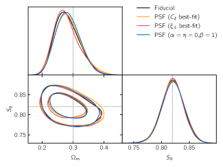
Figure 19: Impact of PSF contamination of the measured shear spectra on cosmological constraints. Fixing the values of the PSF model parameters ($\alpha$, $\beta$ and $\eta$) at the best-fit values inferred from power spectra (blue contours) or two-point functions (red), and at the expected values (orange), we contaminate a noiseless data vector using the model in eq. 36 and compare cosmological constraints to those obtained from the noiseless data vector (black).

Finally, we propagate the PSF bias in eq. 35 to compute the expected contamination of the shear power spectra using the model of eq. 36, in order to test its impact on cosmology. We do so using the best-fit values for the $\alpha$, $\beta$ and $\eta$ parameters from our analysis in harmonic space, the best-fit from the real space analysis in Amon et al. (2022) and the expected values $\alpha=\eta=0$ and $\beta=1$, consistent with non-tomographic results from Jarvis et al. (2021). Figure 19 shows that the impact on cosmological constraints is negligible.

Appendix B Validation on synthetic data

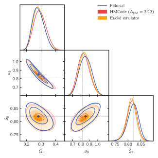
Figure 20: Test of the impact of the non-linear matter power spectrum on cosmological constraints. We analyze three synthetic data vectors with the fiducial model using HaloFit and fiducial scale cuts. Constraints obtained from the fiducial data vector are shown in blue, with the mean of the posterior shown by the blue cross. These constraints are compared to those obtained from data vectors computed with HMCode (red, $A_{\rm HM}=3.13$) and the Euclid Emulator (orange). The innermost contours (underlined in dashed lines) encompass the mean of the fiducial posterior.

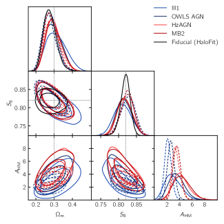
Figure 21: Validation of the baryonic feedback modeling with HMCode. The four colored posteriors are obtained from shear power spectra that include the effect of baryons as predicted by four hydrodynamical simulations (see fig. 5). Solid (dashed) lines were obtained using the scale cuts at $k_{\rm max}=$3\text{\,}\mathrm{\mathit{h}}\text{\,}{\mathrm{Mpc}}^{-1}$$ ($k_{\rm max}=$5\text{\,}\mathrm{\mathit{h}}\text{\,}{\mathrm{Mpc}}^{-1}$$). Despite preferring very different values of $A_{\rm HM}$ (the dark matter-only case corresponds to $A_{\rm HM}=3.13$), the cosmology is recovered in all cases. For comparison, the black contours show the posterior obtained from the fiducial data vector analyzed with HaloFit with the scale cuts at $k_{\rm max}=$3\text{\,}\mathrm{\mathit{h}}\text{\,}{\mathrm{Mpc}}^{-1}$$.

This section illustrates the validation of the modeling pipeline on synthetic data, as described in section 4.4.1. Figure 20 shows the impact of the choice for the non-linear matter power spectrum, whereas fig. 21 validates the use of HMCode to probe the small-scale portion of our measurements, based on its robustness to various baryonic feedback prescriptions from four different hydrodynamical simulations.

Appendix C Internal consistency

This section presents a number of tests in parameter (section C.1) and data space (section C.2) for the fiducial run, i.e. using our fiducial $\Lambda$CDM model and scale cuts, and excluding shear ratio information.

C.1 Robustness of cosmological constraints

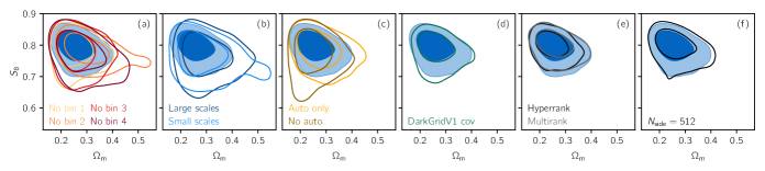
Figure 22: Robustness tests of cosmological constraints, comparing variations in analysis choices to the fiducial constraints in blue. We first repeat the analysis removing part of the data vector, according to (a) redshift bins, (b) scales, and (c) auto-power spectra. We then modify certain parts of the analysis, namely (d) the covariance matrix, (e) the methodology to marginalize over uncertainties in the redshift distributions, and (f) the measurement resolution. See section C.1 for details.

We first perform a series of tests, listed below, to assert the robustness of cosmological constraints presented in section 6.1. Figure 11 presents uni-dimensional marginal distributions for these tests in sections (d) and (e). We also show the two-dimensional marginal distributions in the $(S_{8},\Omega_{\rm m})$ plane in fig. 22, in the following order:

1. Redshift test. Many parts of the cosmological model (including intrinsic alignments) are redshift-dependent by construction, whereas systematic effects may differentially impact the four redshift bins. To test the robustness of the cosmological constraints to such effects, we therefore perform the analysis of cosmic shear power spectra removing one bin at a time (e.g., when removing bin 2, we remove the bin pairs 2,1, 2,2, 3,2 and 4,2 from the data vector), and show contours in fig. 22, panel (a). While contours widen, as expected, and some degeneracies with $A_{\rm TA}$ appear to create some tails in the posteriors, we find an overall excellent agreement, with no visible trend.

2. Large vs small scales. As discussed throughout the paper, the non-linear scales play a crucial role in this analysis, as they contain a significant amount of cosmological information, but are also the most difficult to model. Using our fiducial set of scale cuts, we split the data vector between large and small scales as follows: for each redshift bin pair, we find the multipole $\ell_{\rm thr}$, within the scale cuts ${\ell_{\rm min}\leq\ell\leq\ell_{\rm max}}$, that results in approximately equal signal-to-noise ratio $S/N$ on both sides, i.e. ${S/N_{\ell_{\rm min}\leq\ell\leq\ell_{\rm thr}}\approx S/N_{\ell_{\rm thr}\leq\ell\leq\ell_{\rm max}}}$. This procedure leaves us with 58 and 61 data points for large and small scales, respectively. We find that constraints using either only large scales or only small scales are very similar in width and in very good agreement with each other. The broadening of the posteriors seems related to partial degeneracies with intrinsic alignment parameters, in particular $A_{\rm TT}$. Nevertheless, they are in very good agreement with the constraints from the full analysis.

3. Auto-power spectra. The pseudo-$C_{\ell}$ estimator we use here requires the subtraction of the noise power spectrum, which is estimated analytically from the shape catalog here, following Nicola et al. (2021). In order to evaluate the potential impact of a misestimation, we analyze our data without auto-power spectra, i.e. removing bin pairs 1,1, 2,2, 3,3 and 4,4 from the data vector (No auto), and then using only those pairs (Auto only). We find constraints that are wider but consistent with the full analysis, with no clear indication for an issue with noise spectrum subtraction.

4. Covariance. As described in section 3.3, our covariance matrix is a hybrid matrix that uses NaMaster to evaluate the Gaussian contribution with the effects of the mask and binning properly accounted for, and CosmoLike to evaluate the non-Gaussian contribution, at the fiducial Planck 2018 cosmology. We have also used DarkGridV1 simulations (Zürcher et al., 2022) to obtain an empirical estimate of the covariance matrix, for comparison and validation of our analytic (and therefore noiseless) estimate. We test the impact of this choice by using the empirical covariance in our cosmological analysis, and find that our constraints are almost insensitive to this choice, showing the excellent agreement of the two covariance matrices.

5. HyperRank. Throughout this work, we have employed the fiducial approach over marginalizing over redshift distribution biases, $\Delta z_{a}$’s, in order to account for uncertainty in the redshift distributions. However, the DES Y3 redshift pipeline produced samples of the redshift distributions that can be properly marginalized over using either the MultiRank or HyperRank methods, by sampling, respectively, realizations themselves, or a set of hyperparameters used to rank and select realizations (for details, see Cordero, Harrison et al., 2022). We do so here and find cosmological constraints in excellent agreement with the fiducial analysis, with roughly 15% smaller uncertainty on $S_{8}$ for both techniques.

6. Resolution. As detailed in section 3.1, the pseudo-$C_{\ell}$ estimator is based on pixelized HealPix maps of the shear catalog. However, as discussed in Nicola et al. (2021), the effects of the pixelization of the shear field depend both on the density of galaxies and the chosen resolution. We used a resolution parameter of $N_{\rm side}=1024$, which allows us to probe multipoles up to $\ell\sim 2000$, while yielding a relatively complete mask, without too many empty pixels in the survey area, and with a mean number of galaxies per pixel of around $17.217.5$ for all four bins. This means that we are in the regime where the shear maps are that of the averaged shear field (as opposed to the sampled shear field) and that we may use standard HealPix window functions to correct for the smoothing that has taken place. In order to verify the impact on cosmological constraints, we repeat the measurements, including noise power spectrum and Gaussian covariance estimation, at $N_{\rm side}=512$. We do observe expected differences in the shear power spectra – almost negligible at large scales and growing up to about the size of the error bars at $\ell\sim 1024$, with no clear trend – but find negligible impact on cosmology.

C.2 Internal consistency of data with posterior predictive distributions

Test	Calibrated $p$-value
Goodness-of-fit	0.116
Bin 1 vs no bin 1	0.998
Bin 2 vs no bin 2	0.020
Bin 3 vs no bin 3	0.080
Bin 4 vs no bin 4	0.876
Small vs large scales	0.395
Large vs small scales	0.212

Table 3: Internal consistency tests using the posterior predictive distribution method from Doux et al. (2020). See section C.2 for details.

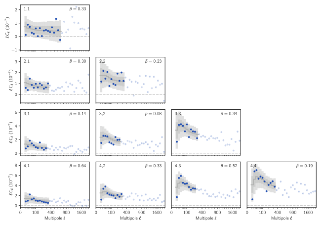
Figure 23: Goodness-of-fit test for the fiducial run using the posterior predictive distribution (PPD) methodology of Doux et al. (2020). The data is shown by the blue circles, which are filled for data points within fiducial scale cuts. The gray line shows the mean of the PPD realizations, whereas the gray bands show the and percentiles of the PPD. The calibrated $p$-value for each panel is shown in the upper right corner.

Bin 1 vs no bin 1
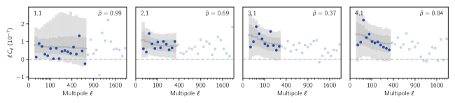
Bin 2 vs no bin 2
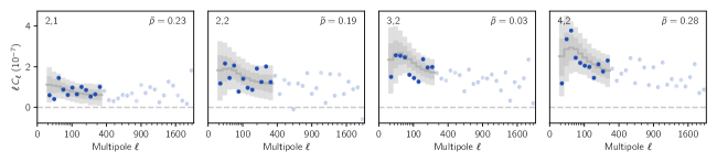
Bin 3 vs no bin 3
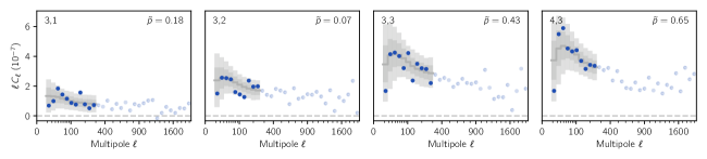
Bin 4 vs no bin 4

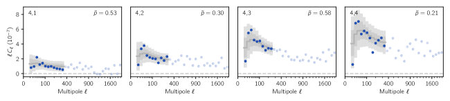
Figure 24: Internal consistency of the four redshift bins (removing one at a time) with the PPD in gray and data in blue. See fig. 23 for details.

We apply the methodology developed of Doux et al. (2020) based on the posterior predictive distribution (PPD) to test the internal consistency of our data. In a nutshell, the method uses a parameter posterior sample and compares simulated realizations of the data vector drawn from the likelihood at these parameter values to the observed data vector. The test is subsequently calibrated using simulated data vectors, to correct for posterior volume effects, as detailed in Doux et al. (2020).

We first perform a goodness-of-fit test, where the posterior sample comes from the fiducial run, and simulated realizations are independent of the observed data, and find a calibrated $p$-value of 11.6%. The PPD samples are shown in gray in fig. 23 along with the observed data in blue.

We then perform consistency tests of the type A vs B, i.e. where we divide the data in two disjoint parts $A$ and $B$, use $B$ to obtain a posterior sample, and generate from those samples realizations of $A$ to be compared to the real data, in a way that accounts for the correlation between $A$ and $B$. Specifically, we split the data according to redshift bins and scales, using the same splits as in item a and item b of the previous section. We illustrate the redshift consistency test in fig. 24 and summarize the results in table 3, finding no indication of inconsistency.

Appendix D Full posterior distribution

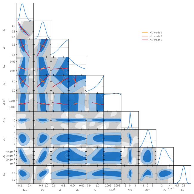
Figure 25: Posterior (in blue) and prior (in gray) distributions for the fiducial $\Lambda$CDM constraints from DES Y3 shear power spectra (without shear ratios) presented in section 6.1, showing cosmological and intrinsic alignment parameters (note that the ranges are adjusted to the posterior for readability). Although we sample over $A_{\rm s}$ with a flat prior, we apply the Karhunen–Loève (KL) decomposition (Raveri & Hu, 2019; Raveri et al., 2020; Raveri & Doux, 2021) in the space of $\quantity{\log\Omega_{\rm m},\log\sigma_{8},\log h,\log\Omega_{\rm b},\log n_{\rm s},\log\Omega_{\nu}h^{2}}$. The best constrained directions in this parameter space, corresponding to the first three modes of the KL decomposition, are represented in yellow, orange and red.

Figure 25 shows the prior and posterior distributions for the fiducial constraints presented in section 6.1 (without shear ratios). We also perform a Karhunen–Loève (KL) decomposition (Raveri & Hu, 2019; Raveri et al., 2020; Raveri & Doux, 2021; Dacunha et al., 2021) in order to determine the directions, in parameter space, that are best constrained by the data, as quantified by the improvement between the prior and the posterior. We use the tensiometer package and work in the space of $\quantity{\log\Omega_{\rm m},\log\sigma_{8},\log h,\log\Omega_{\rm b},\log n_{\rm s},\log\Omega_{\nu}h^{2}}$ in order to express the KL modes as power laws in the original parameters. We find that the three first KL modes are the following (the improvements are in parentheses):

$$\quantity(\frac{\Omega_{\rm m}}{0.255})^{0.521}\quantity(\frac{\sigma_{8}}{0.857}) =1.000\pm 0.116, (978.7\%)$$ (40)

$$\quantity(\frac{\Omega_{\rm m}}{0.255})\quantity(\frac{\sigma_{8}}{0.857})^{-1.219}\quantity(\frac{n_{\rm s}}{1.003})^{2.651} =1.000\pm 0.868, (202.5\%)$$ (41)

$$\quantity(\frac{\Omega_{\rm m}}{0.255})^{-0.149}\quantity(\frac{h}{0.774})\quantity(\frac{n_{\rm s}}{1.003})^{1.681} =1.000\pm 0.426. (77.3\%)$$ (42)

The first mode nearly matches the $S_{8}$ parameter, while subsequent modes, with much weaker improvements, include the Hubble constant $h$ and the tilt of the primordial power spectrum $n_{\rm s}$.

Affiliations

¹ Department of Physics and Astronomy, University of Pennsylvania, Philadelphia, PA 19104, USA
² Department of Physics, ETH Zurich, Wolfgang-Pauli-Strasse 16, CH-8093 Zurich, Switzerland
³ Department of Astronomy, University of California, Berkeley, 501 Campbell Hall, Berkeley, CA 94720, USA
⁴ Department of Astronomy/Steward Observatory, University of Arizona, 933 North Cherry Avenue, Tucson, AZ 85721-0065, USA
⁵ ICTP South American Institute for Fundamental Research
Instituto de Física Teórica, Universidade Estadual Paulista, São Paulo, Brazil
⁶ Laboratório Interinstitucional de e-Astronomia - LIneA, Rua Gal. José Cristino 77, Rio de Janeiro, RJ - 20921-400, Brazil
⁷ Kavli Institute for Particle Astrophysics & Cosmology, P. O. Box 2450, Stanford University, Stanford, CA 94305, USA
⁸ Instituto de Física Teórica, Universidade Estadual Paulista, São Paulo, Brazil
⁹ California Institute of Technology, 1200 East California Blvd, MC 249-17, Pasadena, CA 91125, USA
¹⁰ Kavli Institute for Cosmological Physics, University of Chicago, Chicago, IL 60637, USA
¹¹ Department of Physics, Northeastern University, Boston, MA 02115, USA
¹² Laboratory of Astrophysics, École Polytechnique Fédérale de Lausanne (EPFL), Observatoire de Sauverny, 1290 Versoix, Switzerland
¹³ Department of Astronomy and Astrophysics, University of Chicago, Chicago, IL 60637, USA
¹⁴ Institut d’Estudis Espacials de Catalunya (IEEC), 08034 Barcelona, Spain
¹⁵ Institute of Space Sciences (ICE, CSIC), Campus UAB, Carrer de Can Magrans, s/n, 08193 Barcelona, Spain
¹⁶ Department of Physics & Astronomy, University College London, Gower Street, London, WC1E 6BT, UK
¹⁷ Laboratoire de Physique de l’Ecole Normale Supérieure, ENS, Université PSL, CNRS, Sorbonne Université, Université de Paris, Paris, France
¹⁸ Department of Physics, Carnegie Mellon University, Pittsburgh, Pennsylvania 15312, USA
¹⁹ Argonne National Laboratory, 9700 South Cass Avenue, Lemont, IL 60439, USA
²⁰ Department of Physics, University of Michigan, Ann Arbor, MI 48109, USA
²¹ Institute for Astronomy, University of Hawai’i, 2680 Woodlawn Drive, Honolulu, HI 96822, USA
²² Physics Department, 2320 Chamberlin Hall, University of Wisconsin-Madison, 1150 University Avenue Madison, WI 53706-1390
²³ Instituto de Astrofisica de Canarias, E-38205 La Laguna, Tenerife, Spain
²⁴ Universidad de La Laguna, Dpto. Astrofísica, E-38206 La Laguna, Tenerife, Spain
²⁵ Center for Astrophysical Surveys, National Center for Supercomputing Applications, 1205 West Clark St., Urbana, IL 61801, USA
²⁶ Department of Astronomy, University of Illinois at Urbana-Champaign, 1002 W. Green Street, Urbana, IL 61801, USA
²⁷ Physics Department, William Jewell College, Liberty, MO, 64068
²⁸ Department of Physics, Duke University Durham, NC 27708, USA
²⁹ Jodrell Bank Center for Astrophysics, School of Physics and Astronomy, University of Manchester, Oxford Road, Manchester, M13 9PL, UK
³⁰ Lawrence Berkeley National Laboratory, 1 Cyclotron Road, Berkeley, CA 94720, USA
³¹ NSF AI Planning Institute for Physics of the Future, Carnegie Mellon University, Pittsburgh, PA 15213, USA
³² Fermi National Accelerator Laboratory, P. O. Box 500, Batavia, IL 60510, USA
³³ Jet Propulsion Laboratory, California Institute of Technology, 4800 Oak Grove Dr., Pasadena, CA 91109, USA
³⁴ Center for Cosmology and Astro-Particle Physics, The Ohio State University, Columbus, OH 43210, USA
³⁵ Department of Physics, The Ohio State University, Columbus, OH 43210, USA
³⁶ Santa Cruz Institute for Particle Physics, Santa Cruz, CA 95064, USA
³⁷ Kavli Institute for Cosmology, University of Cambridge, Madingley Road, Cambridge CB3 0HA, UK
³⁸ Institut de Física d’Altes Energies (IFAE), The Barcelona Institute of Science and Technology, Campus UAB, 08193 Bellaterra (Barcelona) Spain
³⁹ University Observatory, Faculty of Physics, Ludwig-Maximilians-Universität, Scheinerstr. 1, 81679 Munich, Germany
⁴⁰ Department of Physics, University of Oxford, Denys Wilkinson Building, Keble Road, Oxford OX1 3RH, UK
⁴¹ School of Physics and Astronomy, Cardiff University, CF24 3AA, UK
⁴² Department of Astronomy, University of Geneva, ch. d’Écogia 16, CH-1290 Versoix, Switzerland
⁴³ Department of Physics, University of Arizona, Tucson, AZ 85721, USA
⁴⁴ Department of Physics and Astronomy, Pevensey Building, University of Sussex, Brighton, BN1 9QH, UK
⁴⁵ Instituto de Astrofísica e Ciências do Espaço, Faculdade de Ciências, Universidade de Lisboa, 1769-016 Lisboa, Portugal
⁴⁶ Department of Applied Mathematics and Theoretical Physics, University of Cambridge, Cambridge CB3 0WA, UK
⁴⁷ Perimeter Institute for Theoretical Physics, 31 Caroline St. North, Waterloo, ON N2L 2Y5, Canada
⁴⁸ Department of Physics, Stanford University, 382 Via Pueblo Mall, Stanford, CA 94305, USA
⁴⁹ SLAC National Accelerator Laboratory, Menlo Park, CA 94025, USA
⁵⁰ Instituto de Física Gleb Wataghin, Universidade Estadual de Campinas, 13083-859, Campinas, SP, Brazil
⁵¹ Kavli Institute for the Physics and Mathematics of the Universe (WPI), UTIAS, The University of Tokyo, Kashiwa, Chiba 277-8583, Japan
⁵² Laboratoire de physique des 2 infinis Irène Joliot-Curie, CNRS Université Paris-Saclay, Bât. 100, Faculté des sciences, F-91405 Orsay Cedex, France
⁵³ Centro de Investigaciones Energéticas, Medioambientales y Tecnológicas (CIEMAT), Madrid, Spain
⁵⁴ Brookhaven National Laboratory, Bldg 510, Upton, NY 11973, USA
⁵⁵ Département de Physique Théorique and Center for Astroparticle Physics, Université de Genève, 24 quai Ernest Ansermet, CH-1211 Geneva, Switzerland
⁵⁶ Excellence Cluster Origins, Boltzmannstr. 2, 85748 Garching, Germany
⁵⁷ Max Planck Institute for Extraterrestrial Physics, Giessenbachstrasse, 85748 Garching, Germany
⁵⁸ Universitäts-Sternwarte, Fakultät für Physik, Ludwig-Maximilians Universität München, Scheinerstr. 1, 81679 München, Germany
⁵⁹ Institute for Astronomy, University of Edinburgh, Edinburgh EH9 3HJ, UK
⁶⁰ Cerro Tololo Inter-American Observatory, NSF’s National Optical-Infrared Astronomy Research Laboratory, Casilla 603, La Serena, Chile
⁶¹ Institute of Cosmology and Gravitation, University of Portsmouth, Portsmouth, PO1 3FX, UK
⁶² CNRS, UMR 7095, Institut d’Astrophysique de Paris, F-75014, Paris, France
⁶³ Sorbonne Universités, UPMC Univ Paris 06, UMR 7095, Institut d’Astrophysique de Paris, F-75014, Paris, France
⁶⁴ Astronomy Unit, Department of Physics, University of Trieste, via Tiepolo 11, I-34131 Trieste, Italy
⁶⁵ INAF-Osservatorio Astronomico di Trieste, via G. B. Tiepolo 11, I-34143 Trieste, Italy
⁶⁶ Institute for Fundamental Physics of the Universe, Via Beirut 2, 34014 Trieste, Italy
⁶⁷ Observatório Nacional, Rua Gal. José Cristino 77, Rio de Janeiro, RJ - 20921-400, Brazil
⁶⁸ Hamburger Sternwarte, Universität Hamburg, Gojenbergsweg 112, 21029 Hamburg, Germany
⁶⁹ Department of Physics, IIT Hyderabad, Kandi, Telangana 502285, India
⁷⁰ Institute of Theoretical Astrophysics, University of Oslo. P.O. Box 1029 Blindern, NO-0315 Oslo, Norway
⁷¹ Instituto de Fisica Teorica UAM/CSIC, Universidad Autonoma de Madrid, 28049 Madrid, Spain
⁷² Department of Astronomy, University of Michigan, Ann Arbor, MI 48109, USA
⁷³ Institute of Astronomy, University of Cambridge, Madingley Road, Cambridge CB3 0HA, UK
⁷⁴ School of Mathematics and Physics, University of Queensland, Brisbane, QLD 4072, Australia
⁷⁵ Center for Astrophysics $|$ Harvard & Smithsonian, 60 Garden Street, Cambridge, MA 02138, USA
⁷⁶ Australian Astronomical Optics, Macquarie University, North Ryde, NSW 2113, Australia
⁷⁷ Lowell Observatory, 1400 Mars Hill Rd, Flagstaff, AZ 86001, USA
⁷⁸ George P. and Cynthia Woods Mitchell Institute for Fundamental Physics and Astronomy, and Department of Physics and Astronomy, Texas A&M University, College Station, TX 77843, USA
⁷⁹ Institució Catalana de Recerca i Estudis Avançats, E-08010 Barcelona, Spain
⁸⁰ School of Physics and Astronomy, University of Southampton, Southampton, SO17 1BJ, UK
⁸¹ Computer Science and Mathematics Division, Oak Ridge National Laboratory, Oak Ridge, TN 37831

References

- Aihara et al. (2018a) Aihara H., et al., 2018a, PASJ, 70, S4
- Aihara et al. (2018b) Aihara H., et al., 2018b, PASJ, 70, S8
- Akeson et al. (2019) Akeson R., et al., 2019, arXiv e-prints, p. arXiv:1902.05569
- Alonso et al. (2019) Alonso D., Sanchez J., Slosar A., LSST Dark Energy Science Collaboration 2019, MNRAS, 484, 4127
- Amodeo et al. (2021) Amodeo S., et al., 2021, Phys. Rev. D, 103, 063514
- Amon et al. (2022) Amon A., et al., 2022, Phys. Rev. D, 105, 023514
- Asgari & Heymans (2019) Asgari M., Heymans C., 2019, MNRAS, 484, L59
- Asgari et al. (2017) Asgari M., Heymans C., Blake C., Harnois-Deraps J., Schneider P., Van Waerbeke L., 2017, MNRAS, 464, 1676
- Asgari et al. (2019) Asgari M., et al., 2019, A&A, 624, A134
- Asgari et al. (2021) Asgari M., et al., 2021, A&A, 645, A104
- Astropy Collaboration et al. (2013) Astropy Collaboration et al., 2013, A&A, 558, A33
- Astropy Collaboration et al. (2018) Astropy Collaboration et al., 2018, AJ, 156, 123
- Bacon et al. (2000) Bacon D. J., Refregier A. R., Ellis R. S., 2000, MNRAS, 318, 625
- Bartelmann (2010) Bartelmann M., 2010, Classical and Quantum Gravity, 27, 233001
- Becker (2013) Becker M. R., 2013, MNRAS, 435, 115
- Becker & Rozo (2016) Becker M. R., Rozo E., 2016, MNRAS, 457, 304
- Blazek et al. (2019) Blazek J. A., MacCrann N., Troxel M. A., Fang X., 2019, Phys. Rev. D, 100, 103506
- Bridle & King (2007) Bridle S., King L., 2007, New Journal of Physics, 9, 444
- Bridle et al. (2009) Bridle S., et al., 2009, Annals of Applied Statistics, 3, 6
- Buchs et al. (2019) Buchs R., et al., 2019, MNRAS, 489, 820
- Camacho et al. (2021) Camacho H., et al., 2021, arXiv e-prints, p. arXiv:2111.07203
- Castro et al. (2005) Castro P. G., Heavens A. F., Kitching T. D., 2005, Phys. Rev. D, 72, 023516
- Catelan et al. (2001) Catelan P., Kamionkowski M., Blandford R. D., 2001, MNRAS, 320, L7
- Chang et al. (2018) Chang C., et al., 2018, MNRAS, 475, 3165
- Chisari et al. (2018) Chisari N. E., et al., 2018, MNRAS, 480, 3962
- Chisari et al. (2019) Chisari N. E., et al., 2019, ApJS, 242, 2
- Cordero et al. (2022) Cordero J. P., Harrison I., et al., 2022, MNRAS, 511, 2170
- Crittenden et al. (2001) Crittenden R. G., Natarajan P., Pen U.-L., Theuns T., 2001, ApJ, 559, 552
- DES Collaboration (2022) DES Collaboration 2022, Phys. Rev. D, 105, 023520
- Dacunha et al. (2021) Dacunha T., Raveri M., Park M., Doux C., Jain B., 2021, arXiv e-prints, p. arXiv:2112.05737
- DeRose et al. (2021) DeRose J., et al., 2021, arXiv e-prints, p. arXiv:2105.13547
- Dietrich & Hartlap (2010) Dietrich J. P., Hartlap J., 2010, MNRAS, 402, 1049
- Doux et al. (2020) Doux C., et al., 2020, Mon. Not. Roy. Astron. Soc.
- Doux et al. (2021) Doux C., et al., 2021, MNRAS, 503, 3796
- Dubois et al. (2014) Dubois Y., et al., 2014, MNRAS, 444, 1453
- Eifler et al. (2014) Eifler T., Krause E., Schneider P., Honscheid K., 2014, MNRAS, 440, 1379
- Euclid Collaboration et al. (2019) Euclid Collaboration et al., 2019, MNRAS, 484, 5509
- Everett et al. (2022) Everett S., et al., 2022, ApJS, 258, 15
- Flaugher (2005) Flaugher B., 2005, International Journal of Modern Physics A, 20, 3121
- Flaugher et al. (2015) Flaugher B., et al., 2015, AJ, 150, 150
- Foreman-Mackey et al. (2013) Foreman-Mackey D., Hogg D. W., Lang D., Goodman J., 2013, PASP, 125, 306
- Friedrich et al. (2021) Friedrich O., et al., 2021, MNRAS, 508, 3125
- Fu et al. (2014) Fu L., et al., 2014, MNRAS, 441, 2725
- García-García et al. (2019) García-García C., Alonso D., Bellini E., 2019, J. Cosmology Astropart. Phys., 2019, 043
- Gatti et al. (2021a) Gatti M., et al., 2021a, arXiv e-prints, p. arXiv:2108.01600
- Gatti et al. (2021b) Gatti M., et al., 2021b, arXiv e-prints, p. arXiv:2110.10141
- Gatti et al. (2021c) Gatti M., Sheldon E., et al., 2021c, MNRAS, 504, 4312
- Gatti et al. (2022) Gatti M., Giannini G., et al., 2022, MNRAS, 510, 1223
- Górski et al. (2005) Górski K. M., Hivon E., Banday A. J., Wandelt B. D., Hansen F. K., Reinecke M., Bartelmann M., 2005, ApJ, 622, 759
- Grain et al. (2009) Grain J., Tristram M., Stompor R., 2009, Phys. Rev. D, 79, 123515
- Hamana et al. (2020) Hamana T., et al., 2020, PASJ, 72, 16
- Hamana et al. (2022) Hamana T., Hikage C., Oguri M., Shirasaki M., More S., 2022, arXiv e-prints, p. arXiv:2201.12698
- Handley et al. (2015) Handley W. J., Hobson M. P., Lasenby A. N., 2015, MNRAS, 450, L61
- Harnois-Déraps et al. (2021) Harnois-Déraps J., Martinet N., Castro T., Dolag K., Giblin B., Heymans C., Hildebrandt H., Xia Q., 2021, MNRAS, 506, 1623
- Harris et al. (2020) Harris C. R., et al., 2020, Nature, 585, 357
- Hartley et al. (2022) Hartley W. G., Choi A., et al., 2022, MNRAS, 509, 3547
- Heymans et al. (2006) Heymans C., et al., 2006, MNRAS, 368, 1323
- Hikage et al. (2011) Hikage C., Takada M., Hamana T., Spergel D., 2011, MNRAS, 412, 65
- Hikage et al. (2019) Hikage C., et al., 2019, PASJ, 71, 43
- Hildebrandt et al. (2017) Hildebrandt H., et al., 2017, MNRAS, 465, 1454
- Hirata & Seljak (2004) Hirata C. M., Seljak U., 2004, Phys. Rev. D, 70, 063526
- Hivon et al. (2002) Hivon E., Górski K. M., Netterfield C. B., Crill B. P., Prunet S., Hansen F., 2002, ApJ, 567, 2
- Howlett et al. (2012) Howlett C., Lewis A., Hall A., Challinor A., 2012, J. Cosmology Astropart. Phys., 2012, 027
- Huang et al. (2019) Huang H.-J., Eifler T., Mandelbaum R., Dodelson S., 2019, MNRAS, 488, 1652
- Huang et al. (2021) Huang H.-J., et al., 2021, MNRAS, 502, 6010
- Huff & Mandelbaum (2017) Huff E., Mandelbaum R., 2017, arXiv e-prints, p. arXiv:1702.02600
- Huff et al. (2014) Huff E. M., Eifler T., Hirata C. M., Mandelbaum R., Schlegel D., Seljak U., 2014, MNRAS, 440, 1322
- Hunter (2007) Hunter J. D., 2007, Computing in Science and Engineering, 9, 90
- Ivezić et al. (2019) Ivezić Ž., et al., 2019, ApJ, 873, 111
- Jain & Seljak (1997) Jain B., Seljak U., 1997, ApJ, 484, 560
- Jarvis (2015) Jarvis M., 2015, TreeCorr: Two-point correlation functions (ascl:1508.007)
- Jarvis et al. (2021) Jarvis M., et al., 2021, MNRAS, 501, 1282
- Jee et al. (2013) Jee M. J., Tyson J. A., Schneider M. D., Wittman D., Schmidt S., Hilbert S., 2013, ApJ, 765, 74
- Jee et al. (2016) Jee M. J., Tyson J. A., Hilbert S., Schneider M. D., Schmidt S., Wittman D., 2016, ApJ, 824, 77
- Jeffrey et al. (2021a) Jeffrey N., Alsing J., Lanusse F., 2021a, MNRAS, 501, 954
- Jeffrey et al. (2021b) Jeffrey N., Gatti M., et al., 2021b, MNRAS, 505, 4626
- Joudaki et al. (2017) Joudaki S., et al., 2017, MNRAS, 465, 2033
- Kaiser (1992) Kaiser N., 1992, ApJ, 388, 272
- Kaiser (1998) Kaiser N., 1998, ApJ, 498, 26
- Kaiser et al. (2000) Kaiser N., Wilson G., Luppino G. A., 2000, arXiv e-prints, pp astro–ph/0003338
- Khandai et al. (2015) Khandai N., Di Matteo T., Croft R., Wilkins S., Feng Y., Tucker E., DeGraf C., Liu M.-S., 2015, MNRAS, 450, 1349
- Kilbinger et al. (2017) Kilbinger M., et al., 2017, MNRAS, 472, 2126
- Kitching et al. (2012) Kitching T. D., et al., 2012, MNRAS, 423, 3163
- Kitching et al. (2017) Kitching T. D., Alsing J., Heavens A. F., Jimenez R., McEwen J. D., Verde L., 2017, MNRAS, 469, 2737
- Köhlinger et al. (2017) Köhlinger F., et al., 2017, MNRAS, 471, 4412
- Krause & Eifler (2017) Krause E., Eifler T., 2017, MNRAS, 470, 2100
- Krause & Hirata (2010) Krause E., Hirata C. M., 2010, A&A, 523, A28
- Krause et al. (2021) Krause E., et al., 2021, arXiv e-prints, p. arXiv:2105.13548
- Kuijken et al. (2015) Kuijken K., et al., 2015, MNRAS, 454, 3500
- Lam et al. (2021) Lam S. K., et al., 2021, numba/numba: Version 0.54.0, doi:10.5281/zenodo.5524874
- Laureijs et al. (2012) Laureijs R., et al., 2012, in Clampin M. C., Fazio G. G., MacEwen H. A., Oschmann Jacobus M. J., eds, Society of Photo-Optical Instrumentation Engineers (SPIE) Conference Series Vol. 8442, Space Telescopes and Instrumentation 2012: Optical, Infrared, and Millimeter Wave. p. 84420T, doi:10.1117/12.926496
- Lawrence et al. (2017) Lawrence E., et al., 2017, ApJ, 847, 50
- Lewis (2019) Lewis A., 2019, arXiv e-prints, p. arXiv:1910.13970
- Lewis et al. (2000) Lewis A., Challinor A., Lasenby A., 2000, ApJ, 538, 473
- Lewis et al. (2001) Lewis A., Challinor A., Turok N., 2001, Phys. Rev. D, 65, 023505
- Limber (1953) Limber D. N., 1953, ApJ, 117, 134
- LoVerde & Afshordi (2008) LoVerde M., Afshordi N., 2008, Phys. Rev. D, 78, 123506
- Loureiro et al. (2021) Loureiro A., et al., 2021, arXiv e-prints, p. arXiv:2110.06947
- MacCrann et al. (2022) MacCrann N., et al., 2022, MNRAS, 509, 3371
- Mackey et al. (2002) Mackey J., White M., Kamionkowski M., 2002, MNRAS, 332, 788
- Mandelbaum (2018) Mandelbaum R., 2018, ARA&A, 56, 393
- Mandelbaum et al. (2014) Mandelbaum R., et al., 2014, ApJS, 212, 5
- Martinelli et al. (2021) Martinelli M., et al., 2021, A&A, 649, A100
- Martinet et al. (2018) Martinet N., et al., 2018, MNRAS, 474, 712
- Massey et al. (2007) Massey R., et al., 2007, MNRAS, 376, 13
- Mead et al. (2015) Mead A. J., Peacock J. A., Heymans C., Joudaki S., Heavens A. F., 2015, MNRAS, 454, 1958
- Mead et al. (2021) Mead A. J., Brieden S., Tröster T., Heymans C., 2021, MNRAS, 502, 1401
- Myles et al. (2021) Myles J., Alarcon A., et al., 2021, MNRAS, 505, 4249
- Nicola et al. (2021) Nicola A., García-García C., Alonso D., Dunkley J., Ferreira P. G., Slosar A., Spergel D. N., 2021, J. Cosmology Astropart. Phys., 2021, 067
- Pandey et al. (2021) Pandey S., et al., 2021, arXiv e-prints, p. arXiv:2108.01601
- Planck Collaboration et al. (2020) Planck Collaboration et al., 2020, A&A, 641, A6
- Porredon et al. (2021) Porredon A., et al., 2021, Phys. Rev. D, 103, 043503
- Potter et al. (2017) Potter D., Stadel J., Teyssier R., 2017, Computational Astrophysics and Cosmology, 4, 2
- Raveri & Doux (2021) Raveri M., Doux C., 2021, Phys. Rev. D, 104, 043504
- Raveri & Hu (2019) Raveri M., Hu W., 2019, Phys. Rev. D, 99, 043506
- Raveri et al. (2020) Raveri M., Zacharegkas G., Hu W., 2020, Phys. Rev. D, 101, 103527
- Rowe (2010) Rowe B., 2010, MNRAS, 404, 350
- Samuroff et al. (2019) Samuroff S., et al., 2019, MNRAS, 489, 5453
- Sánchez et al. (2021) Sánchez C., Prat J., et al., 2021, arXiv e-prints, p. arXiv:2105.13542
- Schaan et al. (2014) Schaan E., Takada M., Spergel D. N., 2014, Phys. Rev. D, 90, 123523
- Schaan et al. (2021) Schaan E., et al., 2021, Phys. Rev. D, 103, 063513
- Schneider & Teyssier (2015) Schneider A., Teyssier R., 2015, J. Cosmology Astropart. Phys., 2015, 049
- Schneider et al. (2002) Schneider P., van Waerbeke L., Mellier Y., 2002, A&A, 389, 729
- Schneider et al. (2019) Schneider A., Teyssier R., Stadel J., Chisari N. E., Le Brun A. M. C., Amara A., Refregier A., 2019, J. Cosmology Astropart. Phys., 2019, 020
- Schneider et al. (2020) Schneider A., Stoira N., Refregier A., Weiss A. J., Knabenhans M., Stadel J., Teyssier R., 2020, J. Cosmology Astropart. Phys., 2020, 019
- Scoville et al. (2007) Scoville N., et al., 2007, ApJS, 172, 1
- Secco et al. (2022) Secco L. F., Samuroff S., et al., 2022, Phys. Rev. D, 105, 023515
- Semboloni et al. (2006) Semboloni E., et al., 2006, A&A, 452, 51
- Sevilla-Noarbe et al. (2021) Sevilla-Noarbe I., et al., 2021, ApJS, 254, 24
- Sheldon & Huff (2017) Sheldon E. S., Huff E. M., 2017, ApJ, 841, 24
- Smith (2006) Smith K. M., 2006, Phys. Rev. D, 74, 083002
- Smith et al. (2003) Smith R. E., et al., 2003, MNRAS, 341, 1311
- Springel (2005) Springel V., 2005, MNRAS, 364, 1105
- Springel et al. (2006) Springel V., Frenk C. S., White S. D. M., 2006, Nature, 440, 1137
- Takada & Jain (2003) Takada M., Jain B., 2003, MNRAS, 340, 580
- Takada & Jain (2009) Takada M., Jain B., 2009, MNRAS, 395, 2065
- Takahashi et al. (2012) Takahashi R., Sato M., Nishimichi T., Taruya A., Oguri M., 2012, ApJ, 761, 152
- Tegmark & Zaldarriaga (2002) Tegmark M., Zaldarriaga M., 2002, Phys. Rev. D, 66, 103508
- The Dark Energy Survey Collaboration (2005) The Dark Energy Survey Collaboration 2005, arXiv e-prints, pp astro–ph/0510346
- Tröster et al. (2021) Tröster T., et al., 2021, arXiv e-prints, p. arXiv:2109.04458
- Troxel et al. (2018) Troxel M. A., et al., 2018, Phys. Rev. D, 98, 043528
- Van Waerbeke et al. (2000) Van Waerbeke L., et al., 2000, A&A, 358, 30
- Virtanen et al. (2020) Virtanen P., et al., 2020, Nature Methods, 17, 261
- Vogelsberger et al. (2014) Vogelsberger M., et al., 2014, MNRAS, 444, 1518
- Wittman et al. (2000) Wittman D. M., Tyson J. A., Kirkman D., Dell’Antonio I., Bernstein G., 2000, Nature, 405, 143
- Wittman et al. (2002) Wittman D. M., et al., 2002, in Tyson J. A., Wolff S., eds, Society of Photo-Optical Instrumentation Engineers (SPIE) Conference Series Vol. 4836, Survey and Other Telescope Technologies and Discoveries. pp 73–82 (arXiv:astro-ph/0210118), doi:10.1117/12.457348
- Xavier et al. (2016) Xavier H. S., Abdalla F. B., Joachimi B., 2016, MNRAS, 459, 3693
- Yang et al. (2011) Yang X., Kratochvil J. M., Wang S., Lim E. A., Haiman Z., May M., 2011, Phys. Rev. D, 84, 043529
- Zonca et al. (2019) Zonca A., Singer L., Lenz D., Reinecke M., Rosset C., Hivon E., Gorski K., 2019, The Journal of Open Source Software, 4, 1298
- Zuntz et al. (2015) Zuntz J., et al., 2015, Astronomy and Computing, 12, 45
- Zürcher et al. (2021) Zürcher D., Fluri J., Sgier R., Kacprzak T., Refregier A., 2021, J. Cosmology Astropart. Phys., 2021, 028
- Zürcher et al. (2022) Zürcher D., et al., 2022, MNRAS,
- de Jong et al. (2013) de Jong J. T. A., et al., 2013, The Messenger, 154, 44
- van Daalen et al. (2011) van Daalen M. P., Schaye J., Booth C. M., Dalla Vecchia C., 2011, MNRAS, 415, 3649