The X-ray coronae in NuSTAR bright active galactic nuclei

Abstract

We present systematic and uniform analysis of NuSTAR data with 10–78 keV S/N $>$ 50, of a sample of 60 SWIFT BAT selected AGNs, 10 of which are radio-loud. We measure their high energy cutoff $E_{\rm cut}$ or coronal temperature $T_{\rm e}$ using three different spectral models to fit their NuSTAR spectra, and show a threshold in NuSTAR spectral S/N is essential for such measurements. High energy spectral breaks are detected in the majority of the sample, and for the rest strong constraints to $E_{\rm cut}$ or $T_{\rm e}$ are obtained. Strikingly, we find extraordinarily large $E_{\rm cut}$ lower limits ($>400$ keV, up to $>$ 800 keV) in 10 radio-quiet sources, whereas none in the radio-loud sample. Consequently and surprisingly, we find significantly larger mean $E_{\rm cut}$/$T_{\rm e}$ of radio-quiet sources compared with radio-loud ones. The reliability of these measurements are carefully inspected and verified with simulations. We find a strong positive correlation between $E_{\rm cut}$ and photon index $\Gamma$, which can not be attributed to the parameter degeneracy. The strong dependence of $E_{\rm cut}$ on $\Gamma$, which could fully account for the discrepancy of $E_{\rm cut}$ distribution between radio-loud and radio-quiet sources, indicates the X-ray coronae in AGNs with steeper hard X-ray spectra have on average higher temperature and thus smaller opacity. However, no prominent correlation is found between $E_{\rm cut}$ and $\lambda_{\rm edd}$. In the $l$–$\Theta$ diagram, we find a considerable fraction of sources lie beyond the boundaries of forbidden regions due to runaway pair production, posing (stronger) challenges to various (flat) coronal geometries.

1 Introduction

The generally accepted disc-corona paradigm illustrates that the powerful hard X-ray emission universally found in active galactic nuclei (AGNs) is produced in the so-called corona (e.g., Haardt & Maraschi, 1991, 1993). In this scenario the UV/optical photons from the accretion disk are upscattered to X-ray band through inverse Compton process by the hot electrons in the corona. However the physical nature of the corona remains yet unclear. Particular matters of concern, for instance, include the location and geometry of the corona (Fabian et al., 2009; Alston et al., 2020), the underlying mechanism for X-ray spectra variability in individual sources (e.g. Wu et al., 2020), potential interactions within the corona like pair-production (Fabian et al., 2015), and the relation between coronal and blackhole properties (Ricci et al., 2018; Hinkle & Mushotzky, 2021).

One of the most fundamental physical parameters of the corona is the temperature $kT_{\rm e}$. The typical X-ray spectrum produced by the inverse Compton scattering within the corona is a power-law continuum, with a high energy cutoff. Such a cutoff ($E_{\rm cut}$) is a direct indicator of the coronal temperature, with $E_{\rm cut}$ $\sim$ 2 $kT_{\rm e}$ or 3 $kT_{\rm e}$ for an optically thin or thick corona (Petrucci et al., 2001). The Nuclear Spectroscopic Telescope Array (NuSTAR; Harrison et al., 2013) is the first hard X-ray telescope with direct-imaging capability above 10 keV. With its broad spectral coverage of 3–78 keV, NuSTAR  has enabled the measurements (or lower limits) of $E_{\rm cut}$/$kT_{\rm e}$ in a number of AGNs (e.g., Ballantyne et al., 2014; Matt et al., 2015; Ursini et al., 2016; Kamraj et al., 2018; Tortosa et al., 2018; Molina et al., 2019; Rani et al., 2019; Panagiotou & Walter, 2020; Porquet et al., 2021; Hinkle & Mushotzky, 2021; Akylas & Georgantopoulos, 2021; Kamraj et al., 2022). Meanwhile, variations of $E_{\rm cut}$/$T_{\rm e}$ are also reported in a few individual sources (e.g., Keek & Ballantyne, 2016; Zhang et al., 2018; Kang et al., 2021).

However, even with NuSTAR spectra, the measurements of $E_{\rm cut}$/$kT_{\rm e}$ are highly challenging for most AGNs, primarily due to the limited spectral quality at the high energy end. In many sample studies, only poorly constrained lower limits could be obtained for the dominant fraction of sources in the samples (e.g. Ricci et al., 2018; Kamraj et al., 2018; Panagiotou & Walter, 2020; Kamraj et al., 2022), hindering further reliable statistical studies, e.g., to probe the dependence of $E_{\rm cut}$/$kT_{\rm e}$ on other physical parameters. Meanwhile, the $E_{\rm cut}$ measurements are often sensitive to the choice of spectral models. From this perspective, it is essential to perform uniform spectral fitting to a statistical sample with various models adopted.

Recently, we uniformly analyzed the NuSTAR spectra for a sample of 28 radio-loud AGNs (Kang et al., 2020). We found that $E_{\rm cut}$ could be ubiquitously (9 out 11) detected in radio AGNs with NuSTAR net counts above 10^4.5, and the ubiquitous detections of $E_{\rm cut}$ in FR II galaxies indicate their X-ray emission is dominated by the thermal corona, instead of the jet. While for sources with lower NuSTAR counts, only a minor fraction of $E_{\rm cut}$ detections (4 out of 17) were achieved. This motivates this work to perform systematic analyses of NuSTAR spectra of a sample of radio-quiet AGNs with sufficiently high signal to noise ratio of NuSTAR spectra (to avoid too many lower limits), and to statistically study the distribution of $E_{\rm cut}$/$kT_{\rm e}$, its dependence on other parameters, and the comparison with radio-loud AGNs.

The paper is organized as follows. In §2, we present the sample selection and data reduction. The spectral fitting process as well as the fitting results are shown in §3. Discussions are put in §4.

2 The Sample and Data Reduction

We match the 817 Seyfert galaxies in the 105-month BAT catalogue (Oh et al., 2018) with the archival NuSTAR observations (as of October 2020). We drop observations with exposure time $<$ 3 ks, or with total net counts (FPMA + FPMB) $<$ 3000, for which no valid $E_{\rm cut}$ measurement can be obtained. We exclude a few exposures contaminated by solar activity or other unknown issues (through visually checking the images). Furthermore, we exclude Compton-thick or heavily obscured sources (with n${}_{\rm H}>10^{23}cm^{-2}$ fitted with a simple neutral absorber model). Based on the spectral fitting introduced in §3, several observations with extremely hard spectra (photon index $\Gamma<$ 1.3) or poor fitting statistics ($\chi^{2}_{\nu}>$ 1.2), for which more complicated spectral models would be required, are also dropped. After these steps, 198 sources are kept, including 20 radio-loud sources and 178 radio-quiet sources.

Kang et al. (2020) presented a radio-loud sample of 28 sources with NuSTAR exposures, 20 of which are included in the sample described above, while the rest 8 sources are classified as “beamed AGN” in the BAT catalog (Oh et al., 2018). Among them, 3C 279 is later found to be a jet-dominated blazar (e.g., Blinov et al., 2021) and is excluded from this work. Besides, we drop NGC 1275 (3C 84) due to the strong contamination from the diffuse thermal emission of the Perseus cluster to its spectra (Rani et al., 2018).

For sources with multiple NuSTAR exposures observations, the ones with the most 3–78 keV net counts are adopted. Raw data are reduced using the NuSTAR Data Analysis Software within the latest version of HEASoft package (version 6.28), with calibration files CALDB version 20201101. These new versions of HEASoft and CALDB are applied to revise the recently noticed low-energy effective area issue of FPMA (Madsen et al., 2020), which may partly account for the different fitting results from previous literature. The standard pipeline nupipeline is used to generate the calibrated and cleaned event files. Following Kang et al. (2020, 2021), each source spectrum is extracted in a circular region with a radius of 60″ centered on each source using nuproduct, while the background spectrum is derived using NUSKYBGD (Wik et al., 2014), handling the spatially non-uniform background. As the last step, spectra are rebinned using grppha to achieve a minimum of 50 counts bin^-1.

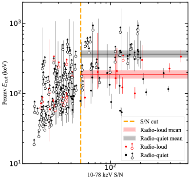
(a)

Figure 1: $E_{\rm cut}$ or lower limits from model $pexrav$ vs. 10–78 keV NuSTAR (FPMA) spectral S/N. A cut at 50 is adopted, sources below which are dropped. Mean values for radio-quiet and radio-loud samples are calculated using Kaplan-Meier estimator within ASURV in logarithm space (hereafter the same), and the shaded regions plot the 1$\sigma$ scatter of the mean derived through bootstrapping the corresponding sample (hereafter the same).

We note the $E_{\rm cut}$ measurement is profoundly affected by the quality of the spectra, particularly at the high energy band. In Fig. 1 we plot the best-fit $E_{\rm cut}$ (or lower limits, derived through fitting NuSTAR spectra with $pexrav$, see §3) for the 178 radio-quiet and 26 radio-loud AGNs, versus 10–78 keV S/N of NuSTAR FPMA net counts. Clearly the measurements of $E_{\rm cut}$ for sources with low 10–78 keV S/N are dominated by poorly constrained lower limits for both radio-loud and radio-quiet sources. The lower limits systematically and significantly increase with 10–78 keV S/N at S/N $<$ 50 and the increase saturates at S/N $>$ 50. This indicates a threshold in S/N is essential to derive effective constraints to $E_{\rm cut}$. Thus in this work we focus only on sources with 10–78 keV NuSTAR spectral S/N $>$ 50, including 50 radio-quiet and 10 radio-loud sources (see Tab. 1).

We notice some NuSTAR observations have joint exposures from other missions like XMM-Newton or Swift. Those data are not included in this work mainly because different photon indices have been found between the spectra of NuSTAR and other missions (e.g., Cappi et al., 2016; Middei et al., 2019; Ponti et al., 2018), which may lead to significantly biased $E_{\rm cut}$/$kT_{\rm e}$ measurements. Such discrepancy is likely caused by the imperfect inter-instrument calibration, while the fact that joint exposures are not completely simultaneous (different start/end time, different livetime distribution) can also play a part due to rapid spectral variations. Significant loss of the valuable NuSTAR exposure time would be unavoidable if we require perfect simultaneity between NuSTAR and exposures from other missions. Considering the $E_{\rm cut}$/$kT_{\rm e}$ measurement is sensitive to the photon index, and to avoid the potential bias due to the fact that only a fraction of the exposures have quasi-simultaneous observations from other various missions, here we perform uniform spectral fitting to NuSTAR spectra alone for the whole sample.

Table 1: Sample Details

Source	obsID	10–78 keV S/N	Log M	Log Lbol14-195keV	Log $\lambda_{\rm edd}$	Log L0.1-200keV	Compactness $l$
			$M_{\odot}$	erg/s		erg/s
Radio-quiet
Mrk 1148	60160028002	51	7.82	45.3	-0.64	44.8	161
Fairall 9	60001130003	111	8.30	45.3	-1.14	44.6	34
NGC 931	60101002002	111	7.29	44.5	-0.96	43.8	59
HB89 0241+622	60160125002	66	8.09	45.6	-0.60	44.6	62
NGC 1566	80301601002	162	5.74	42.5	-1.38	43.1	449
1H 0419-577	60101039002	129	8.07	45.7	-0.46	45.1	181
Ark 120	60001044004	125	8.07	45.1	-1.07	44.5	46
ESO 362-18	60201046002	97	7.42	44.1	-1.41	43.2	11
2MASX J05210136-2521450	60201022002	52	-	-	-	43.8	-
NGC 2110	60061061002	174	9.25	44.6	-2.79	44.2	1.5
MCG +08-11-011	60201027002	187	7.62	45.0	-0.76	44.3	78
MCG +04-22-042	60061092002	51	7.34	44.9	-0.56	44.2	147
Mrk 110	60201025002	213	7.29	45.1	-0.29	44.6	354
NGC 2992	90501623002	190	5.42	43.4	-0.14	43.7	3413
MCG-05-23-016	60001046008	380	5.86	44.4	0.40	43.7	1172
NGC 3227	60202002014	148	6.77	43.6	-1.33	42.9	22
NGC 3516	60002042004	58	7.39	44.5	-1.03	42.7	4.2
HE 1136-2304	80002031003	65	7.62	44.4	-1.40	43.8	26
NGC 3783	60101110002	123	7.37	44.6	-0.90	43.4	20
UGC 06728	60376007002	75	5.66	43.3	-0.51	44.7	21819
2MASX J11454045-1827149	60302002006	63	7.31	45.0	-0.42	44.3	181
NGC 3998	60201050002	63	8.93	42.8	-4.23	41.8	0.01
NGC 4051	60401009002	188	6.13	42.9	-1.34	41.8	8.2
Mrk 766	60001048002	98	6.82	43.8	-1.15	43.3	53
NGC 4593	60001149008	66	6.88	44.0	-1.05	43.2	38
WKK 1263	60160510002	58	8.25	44.7	-1.66	44.2	17
MCG-06-30-015	60001047003	185	5.82	43.8	-0.11	43.2	444
NGC 5273	60061350002	55	6.66	42.5	-2.26	42.3	7.9
4U 1344-60	60201041002	174	7.32	44.5	-0.95	43.7	48
IC 4329A	60001045002	341	7.84	45.1	-0.85	44.3	59
Mrk 279	60160562002	62	7.43	44.8	-0.75	44.2	119
NGC 5506	60061323002	158	5.62	44.1	0.37	43.3	794
NGC 5548	60002044006	123	7.72	44.6	-1.24	44.0	31
WKK 4438	60401022002	71	6.86	44.0	-0.98	43.2	39
Mrk 841	60101023002	51	7.81	45.0	-0.99	44.3	55
AX J1737.4-2907	60301010002	101	-	-	-	44.2	-
2MASXi J1802473-145454	60160680002	52	7.76	45.0	-0.92	44.4	79
ESO 141-G 055	60201042002	124	8.07	45.1	-1.06	44.4	39
2MASX J19373299-0613046	60101003002	77	6.56	43.6	-1.04	43.1	57
NGC 6814	60201028002	188	7.04	43.6	-1.58	42.9	12
Mrk 509	60101043002	228	8.05	45.3	-0.86	44.6	63
SWIFT J212745.6+565636	60402008004	124	7.20 (1)	-	-	43.7	51
NGC 7172	60061308002	127	8.45	44.3	-2.31	43.6	2.8
NGC 7314	60201031002	148	4.99	43.2	0.12	42.7	970
Mrk 915	60002060002	60	7.71	44.5	-1.33	43.7	18
MR 2251-178	60102025004	92	8.44	45.9	-0.66	45.3	126
NGC 7469	60101001014	72	6.96	44.5	-0.60	41.8	1.4
Mrk 926	60201029002	199	8.55	45.7	-1.01	45.0	56
NGC 4579	60201051002	64	7.80	-	-	42.2	0.43
M 81	60101049002	155	7.90	41.3	-4.72	41.1	0.03
Radio-loud
3C 109	60301011004	55	8.30 (2)	47.4	0.98	45.8	539
3C 111	60202061004	112	8.27	45.7	-0.67	44.9	82
3C 120	60001042003	207	7.74	45.3	-0.59	44.7	152
PicA	60101047002	74	7.60 (3)	44.9	-0.79	43.9	38
3C 273	10002020001	391	8.84	47.4	0.41	46.4	641
CentaurusA	60001081002	509	7.74 (4)	43.3	-2.61	42.7	1.6
3C 382	60001084002	133	8.19	45.7	-0.58	45.0	116
3C 390.3	60001082003	115	8.64	45.8	-0.99	45.1	50
4C 74.26	60001080006	131	9.60	46.1	-1.67	45.4	12
IGR J21247+5058	60301005002	175	7.63	44.9	-0.85	44.5	145

Note. — Sources are ordered by BAT ID. The 10–78 keV signal-to-noise ratios are calculated using FPMA spectra. The blackhole masses are from Koss et al. (2017), unless marked with a number referring to the following literature.(1) Malizia et al. (2008); (2) McLure et al. (2006); (3) Lewis & Eracleous (2006); (4) Cappellari et al. (2009) . Lbol_14-195keV is the bolometric luminosity estimated by the BAT 14–195 keV flux (Koss et al., 2017) and used for $\lambda_{\rm edd}$ calculation. L_0.1-200keV is the unabsorbed 0.1–200 keV luminosity, extrapolated using the best-fit results of $pexrav$ to NuSTAR spectra and adopting the redshifts from the 105-month BAT catalogue and $H_{0}=70$ km s^-1 Mpc^-1. The compactness parameter $l$ is derived from L_0.1-200keV.

3 Spectral Fitting

Spectral fitting is carried out within the 3–78 keV band using XSPEC (Arnaud, 1996). $\chi^{2}$ statistics is adopted and all the errors together with the upper/lower limits in this paper correspond to 90% confidence level with $\Delta\chi^{2}=2.71$, unless otherwise stated. The relative element abundance is set to the default in XSPEC, given by Anders & Grevesse (1989). For each observation, the spectra of FPMA and FPMB are jointly fitted with a cross-normalization (Madsen et al., 2015a).

In this paper we intend to perform uniform measurements of the $E_{\rm cut}$ / $T_{\rm e}$ for the radio-quiet and radio-loud samples and bring them into comparison. In order to guarantee such comparison is model-independent, various models are employed, including $pexrav$, $relxill$, and $relxillcp$.

$pexrav$ (Magdziarz & Zdziarski, 1995) is the model we used to fit the radio-loud sample in Kang et al. (2020), which fits the spectra with an exponentially cutoff power law plus a neutral reflection component, and is the most widely used model in $E_{\rm cut}$ measurement (e.g., Molina et al., 2019; Rani et al., 2019; Panagiotou & Walter, 2020; Baloković et al., 2020; Kang et al., 2021). For simplicity, the solar element abundance for the reflector and an inclination of cos$i$ = 0.45 are adopted, which are the default values of the model. We allow the photon index $\Gamma$, $E_{\rm cut}$ and the reflection scaling factor $R$ free to vary.

$relxill$ (García et al., 2014) also models the underlying continuum with a cutoff powerlaw, but convolves the reflection component with disc relativistic broadening effect. However, some parameters are hard to constrain even with these high-quality NuSTAR spectra and hence have to be frozen. The inner and outer radius of the accretion disk, $Rin$ and $Rout$, are fixed at 1 ISCO and 400 gravitational radii respectively as the default of the model. Besides we fix the blackhole spin $a=0.998$ and the inclination angle $i=30^{\circ}$. The accretion disk is presumed to be neutral and have the solar iron abundance, with the corresponding parameter $logxi$ and $Afe$ fixed at 0 and 1, respectively. We assume a disk with constant emissivity, setting the emissivity parameter $Index2$ tied with $Index1$. The free parameters include $Index1$, $\Gamma$, $E_{\rm cut}$ and the reflection fraction (with different definition from the $R$ in $pexrav$).

A Comptonization model, $relxillcp$, is also adopted to directly measure the coronal temperature $T_{\rm e}$. $relxillcp$ is a Comptonization version of $relxill$, replacing the cutoff power law with a nthcomp continuum. Other parameters are set in the same way as $relxill$.

Meanwhile, a common component $zphabs$ is added to all three models to represent the intrinsic photoelectric absorption, with the Galactic absorption ignored due to its inappreciable influence on NuSTAR spectra. As for the Fe K$\alpha$ lines, in $relxill$ and $relxillcp$ the continuum reflection component and the Fe K$\alpha$ line are jointly fitted, while a $zgauss$ is added to $pexrav$ to describe the Fe K$\alpha$ line. Since a relativistically broadened Fe K$\alpha$ line can not be well constrained in the majority of observations, we deal with the Gaussian component as follows. In the first place we fix the line at 6.4 keV in the rest frame and the line width at 19 eV (the mean Fe K$\alpha$ line width in AGNs measured with Chandra HETG, Shu et al., 2010) to model a neutral narrow Fe K$\alpha$ line. Then we allow the line width free to vary. If a variable line width prominently improves the fitting ($\Delta\chi^{2}>5$), the corresponding fitting results are adopted.

We summarize below the three models adopted in the XSPEC term and the corresponding free parameters.

• $zphabs*(pexrav+zgauss)$
  Free parameters include absorption column density $n_{\rm H}$, photon index $\Gamma$, high energy cutoff $E_{\rm cut}$ and the strength of the reflection component R.

• $zphabs*relxill$
  $n_{\rm H}$, $\Gamma$, $E_{\rm cut}$, emissivity parameter $Index1$ and the reflection fraction.

• $zphabs*relxillcp$
  Same as $relxill$, except that $E_{\rm cut}$ is replaced with $T_{\rm e}$.

The best-fitting results of the key parameters are shown in Tab. 2. In a few sources the spectral fitting yields very high lower limits of $E_{\rm cut}$, up to 2360 keV (see §4 for further discussion on reliability of such high lower limits of $E_{\rm cut}$). For the two sources with $E_{\rm cut}$ lower limits above 800 keV ($pexrav$ results; NGC 4051, $>$ 2360 keV; NGC 4593, $>$ 1420 keV), we manually and conservatively set their $E_{\rm cut}$ lower limits at 800 keV. Simply adopting their best-fit lower limits would further strengthen the results of this work.

Table 2: Spectral Fitting Results

Source	obsID	$\Gamma^{\rm pexrav}$	$R^{\rm pexrav}$	$E_{\rm cut}^{\rm pexrav}$	$\chi_{\rm pexrav}^{2}/dof$	$E_{\rm cut}^{\rm relxill}$	$\chi_{\rm relxill}^{2}/dof$	$T_{\rm e}^{\rm relxillcp}$	$\chi_{\rm relxillcp}^{2}/dof$
				keV		keV		keV
Radio-quiet
Mrk 1148	60160028002	$1.79_{-0.08}^{+0.13}$	$<0.45$	$113_{-47}^{+427}$	0.91	$>65$	0.92	$>18$	0.92
Fairall 9	60001130003	$1.96_{-0.03}^{+0.06}$	$0.71_{-0.17}^{+0.22}$	$>396$	0.91	$>400$	0.94	$>182$	0.96
NGC 931	60101002002	$1.88_{-0.06}^{+0.06}$	$0.70_{-0.19}^{+0.21}$	$>280$	0.85	$>293$	0.86	$>138$	0.86
HB89 0241+622	60160125002	$1.70_{-0.06}^{+0.06}$	$0.73_{-0.27}^{+0.33}$	$240_{-101}^{+489}$	0.97	$>158$	1.02	$>50$	1.02
NGC 1566	80301601002	$1.84_{-0.04}^{+0.05}$	$0.80_{-0.14}^{+0.15}$	$>434$	0.93	$>511$	0.93	$>173$	0.93
1H 0419-577	60101039002	$1.64_{-0.05}^{+0.06}$	$0.38_{-0.13}^{+0.15}$	$54_{-6}^{+8}$	0.99	$54_{-6}^{+8}$	0.99	$16_{-1}^{+1}$	1.00
Ark 120	60001044004	$1.98_{-0.03}^{+0.03}$	$0.58_{-0.12}^{+0.14}$	$>744$	1.06	$>414$	1.10	$>213$	1.12
ESO 362-18	60201046002	$1.57_{-0.08}^{+0.09}$	$0.58_{-0.22}^{+0.26}$	$133_{-40}^{+91}$	1.03	$135_{-33}^{+92}$	1.08	$>34$	1.09
2MASX J05210136-2521450	60201022002	$2.06_{-0.12}^{+0.15}$	$0.33_{-0.30}^{+0.74}$	$>111$	0.99	$>129$	1.00	$>49$	1.00
NGC 2110	60061061002	$1.67_{-0.03}^{+0.03}$	$<0.03$	$>327$	0.95	$>382$	0.96	$>217$	0.99
MCG +08-11-011	60201027002	$1.81_{-0.02}^{+0.04}$	$0.26_{-0.09}^{+0.10}$	$417_{-154}^{+688}$	1.03	$>302$	1.09	$>244$	1.10
MCG +04-22-042	60061092002	$1.95_{-0.09}^{+0.10}$	$0.59_{-0.33}^{+0.44}$	$>216$	0.87	$>167$	0.88	$>37$	0.88
Mrk 110	60201025002	$1.74_{-0.01}^{+0.01}$	$<0.04$	$160_{-24}^{+35}$	1.05	$159_{-32}^{+43}$	1.10	$57_{-18}^{+54}$	1.11
NGC 2992	90501623002	$1.68_{-0.04}^{+0.04}$	$0.08_{-0.07}^{+0.08}$	$395_{-152}^{+636}$	1.05	$>316$	1.15	$>260$	1.16
MCG -05-23-016	60001046008	$1.72_{-0.02}^{+0.02}$	$0.45_{-0.05}^{+0.05}$	$115_{-9}^{+11}$	1.10	$125_{-8}^{+10}$	1.19	$41_{-3}^{+3}$	1.24
NGC 3227	60202002014	$1.90_{-0.05}^{+0.05}$	$1.21_{-0.19}^{+0.22}$	$342_{-125}^{+417}$	1.01	$>251$	1.01	$>83$	1.01
NGC 3516	60002042004	$1.68_{-0.09}^{+0.09}$	$0.65_{-0.30}^{+0.39}$	$>476$	1.10	$>368$	1.17	$>114$	1.18
HE 1136-2304	80002031003	$1.69_{-0.10}^{+0.10}$	$<0.48$	$169_{-79}^{+871}$	1.00	$160_{-71}^{+573}$	1.00	$>21$	1.01
NGC 3783	60101110002	$1.94_{-0.07}^{+0.07}$	$1.58_{-0.28}^{+0.33}$	$>346$	1.05	$>432$	1.04	$>150$	1.05
UGC 06728	60376007002	$1.80_{-0.10}^{+0.10}$	$0.75_{-0.28}^{+0.33}$	$230_{-108}^{+933}$	1.01	$183_{-62}^{+452}$	1.01	$>26$	1.01
2MASX J11454045-1827149	60302002006	$1.79_{-0.08}^{+0.11}$	$0.43_{-0.27}^{+0.33}$	$109_{-38}^{+124}$	0.88	$105_{-33}^{+98}$	0.88	$29_{-10}^{+44}$	0.89
NGC 3998	60201050002	$1.96_{-0.07}^{+0.08}$	$<0.34$	$>219$	0.96	$>201$	0.97	$>47$	0.97
NGC 4051	60401009002	$2.05_{-0.03}^{+0.03}$	$2.04_{-0.20}^{+0.22}$	$>800$	1.04	$>800$	1.02	$>270$	1.05
Mrk 766	60001048002	$2.30_{-0.07}^{+0.07}$	$1.76_{-0.34}^{+0.40}$	$>200$	1.05	$>352$	1.05	$>157$	1.06
NGC 4593	60001149008	$1.83_{-0.05}^{+0.05}$	$0.63_{-0.21}^{+0.25}$	$>800$	0.99	$>577$	1.00	$>144$	1.02
WKK 1263	60160510002	$1.79_{-0.09}^{+0.09}$	$<0.50$	$>529$	0.86	$>374$	0.86	$>72$	0.87
MCG -06-30-015	60001047003	$2.29_{-0.04}^{+0.02}$	$1.83_{-0.20}^{+0.21}$	$>707$	1.07	$>720$	1.05	$>280$	1.07
NGC 5273	60061350002	$1.90_{-0.11}^{+0.11}$	$1.30_{-0.50}^{+0.66}$	$>467$	1.11	$>362$	1.11	$>85$	1.12
4U 1344-60	60201041002	$1.90_{-0.05}^{+0.05}$	$0.92_{-0.15}^{+0.17}$	$308_{-101}^{+265}$	1.11	$337_{-112}^{+204}$	1.12	$>104$	1.13
IC 4329A	60001045002	$1.72_{-0.02}^{+0.02}$	$0.32_{-0.05}^{+0.05}$	$195_{-27}^{+37}$	1.03	$215_{-33}^{+37}$	1.07	$71_{-15}^{+37}$	1.09
Mrk 279	60160562002	$1.90_{-0.04}^{+0.05}$	$0.19_{-0.17}^{+0.20}$	$>542$	1.01	$>231$	1.07	$>84$	1.07
NGC 5506	60061323002	$1.90_{-0.06}^{+0.05}$	$1.29_{-0.19}^{+0.22}$	$>424$	1.08	$>551$	1.06	$>211$	1.07
NGC 5548	60002044006	$1.69_{-0.06}^{+0.06}$	$0.62_{-0.17}^{+0.19}$	$128_{-30}^{+53}$	0.99	$126_{-28}^{+45}$	1.00	$36_{-8}^{+11}$	1.01
WKK 4438	60401022002	$2.00_{-0.05}^{+0.08}$	$1.11_{-0.33}^{+0.44}$	$>234$	0.92	$>263$	0.93	$>81$	0.94
Mrk 841	60101023002	$1.89_{-0.12}^{+0.06}$	$0.45_{-0.33}^{+0.45}$	$>176$	1.02	$>154$	1.02	$>44$	1.02
AX J1737.4-2907	60301010002	$1.79_{-0.08}^{+0.08}$	$0.94_{-0.25}^{+0.29}$	$75_{-14}^{+23}$	1.05	$112_{-36}^{+95}$	1.04	$35_{-14}^{+184}$	1.04
2MASXi J1802473-145454	60160680002	$1.76_{-0.08}^{+0.09}$	$<0.41$	$>128$	1.03	$>135$	1.08	$>53$	1.08
ESO 141- G 055	60201042002	$1.92_{-0.03}^{+0.03}$	$0.67_{-0.15}^{+0.17}$	$>351$	1.04	$>293$	1.05	$>125$	1.05
2MASX J19373299-0613046	60101003002	$2.45_{-0.11}^{+0.16}$	$2.01_{-0.65}^{+1.39}$	$>143$	0.99	$>217$	1.13	$>137$	1.14
NGC 6814	60201028002	$1.83_{-0.03}^{+0.04}$	$0.46_{-0.10}^{+0.11}$	$>311$	1.06	$371_{-108}^{+318}$	1.10	$>147$	1.11
Mrk 509	60101043002	$1.75_{-0.02}^{+0.02}$	$0.41_{-0.07}^{+0.08}$	$104_{-10}^{+13}$	1.06	$98_{-8}^{+13}$	1.08	$24_{-2}^{+2}$	1.12
SWIFT J212745.6+565636	60402008004	$2.10_{-0.04}^{+0.05}$	$1.77_{-0.33}^{+0.45}$	$56_{-6}^{+7}$	1.06	$63_{-8}^{+11}$	1.07	$21_{-3}^{+8}$	1.07
NGC 7172	60061308002	$1.84_{-0.06}^{+0.06}$	$0.68_{-0.17}^{+0.19}$	$385_{-174}^{+1239}$	1.05	$337_{-137}^{+523}$	1.05	$>54$	1.05
NGC 7314	60201031002	$2.06_{-0.05}^{+0.05}$	$1.18_{-0.19}^{+0.21}$	$>267$	1.05	$>346$	1.07	$>188$	1.07
Mrk 915	60002060002	$1.81_{-0.09}^{+0.10}$	$0.37_{-0.27}^{+0.34}$	$>378$	1.03	$>286$	1.05	$>69$	1.06
MR 2251-178	60102025004	$1.77_{-0.07}^{+0.07}$	$<0.25$	$195_{-75}^{+310}$	1.02	$>117$	1.01	$37_{-12}^{+97}$	1.01
NGC 7469	60101001014	$1.85_{-0.05}^{+0.08}$	$0.41_{-0.21}^{+0.30}$	$>262$	0.88	$>242$	0.89	$>77$	0.89
Mrk 926	60201029002	$1.73_{-0.02}^{+0.02}$	$<0.10$	$323_{-96}^{+241}$	1.05	$292_{-87}^{+178}$	1.11	$>83$	1.11
NGC 4579	60201051002	$1.88_{-0.08}^{+0.04}$	$<0.15$	$>230$	1.02	$>93$	1.08	$>49$	1.08
M 81	60101049002	$1.88_{-0.02}^{+0.02}$	$<0.05$	$358_{-135}^{+538}$	1.00	$225_{-85}^{+233}$	1.10	$>83$	1.11
Radio-loud
3C 109	60301011004	$1.64_{-0.08}^{+0.16}$	$0.32_{-0.24}^{+0.32}$	$87_{-24}^{+86}$	0.95	$88_{-25}^{+97}$	0.96	$30_{-11}^{+60}$	0.97
3C 111	60202061004	$1.70_{-0.04}^{+0.06}$	$<0.08$	$165_{-47}^{+202}$	1.07	$174_{-57}^{+166}$	1.10	$>35$	1.11
3C 120	60001042003	$1.86_{-0.03}^{+0.03}$	$0.40_{-0.08}^{+0.09}$	$300_{-85}^{+188}$	1.01	$289_{-80}^{+138}$	1.02	$>91$	1.02
PicA	60101047002	$1.72_{-0.04}^{+0.04}$	$<0.10$	$202_{-87}^{+527}$	0.98	$161_{-74}^{+754}$	1.00	$>29$	1.01
3C 273	10002020001	$1.62_{-0.01}^{+0.02}$	$0.05_{-0.03}^{+0.03}$	$226_{-26}^{+42}$	1.02	$>237$	1.03	$>79$	1.03
CentaurusA	60001081002	$1.75_{-0.01}^{+0.01}$	$<0.01$	$335_{-56}^{+85}$	1.00	$209_{-24}^{+34}$	1.04	$101_{-24}^{+85}$	1.08
3C 382	60001084002	$1.76_{-0.05}^{+0.04}$	$<0.13$	$>297$	0.95	$>268$	0.98	$>105$	0.98
3C 390.3	60001082003	$1.72_{-0.06}^{+0.06}$	$0.14_{-0.12}^{+0.14}$	$208_{-73}^{+232}$	0.98	$235_{-85}^{+267}$	1.00	$>46$	1.00
4C 74.26	60001080006	$1.80_{-0.04}^{+0.07}$	$0.66_{-0.15}^{+0.18}$	$121_{-22}^{+48}$	0.99	$165_{-42}^{+85}$	1.01	$62_{-23}^{+265}$	1.01
IGR J21247+5058	60301005002	$1.63_{-0.02}^{+0.04}$	$<0.11$	$100_{-15}^{+22}$	1.07	$102_{-16}^{+22}$	1.08	$26_{-3}^{+6}$	1.11

4 Discussion

The best-fit $E_{\rm cut}$ from $pexrav$ is presented in Fig. 1. We plot the $E_{\rm cut}$/$T_{\rm e}$ from the other two models versus 10–78 keV S/N in Fig. 2. Similar to Kang et al. (2020), we find the $E_{\rm cut}$ in this radio-loud sample can be well constrained as long as the spectra have enough S/N. With $pexrav$ we obtain $E_{\rm cut}$ measurements for 9 out 10 radio-loud sources with 10–78 keV S/N $>$ 50. The only radio-loud source without $E_{\rm cut}$ detection is 3C 382, for which $E_{\rm cut}$ detection was reported in another NuSTAR exposure with slightly less NuSTAR net counts than the one adopted in this work.

Table 3: The mean $E_{\rm cut}$/$T_{\rm e}$ of our RQ and RL samples. The last row presents the statistical significance of the difference in the mean value between two samples.

	$pexrav$ $E_{\rm cut}$	$relxill$ $E_{\rm cut}$	$relxillcp$ $T_{\rm e}$
RQ (keV)	$364^{+45}_{-40}$	$390^{+60}_{-52}$	$174^{+23}_{-20}$
RL (keV)	$187^{+27}_{-24}$	$188^{+26}_{-23}$	$72^{+13}_{-11}$
Significance ($\sigma$)	3.6	3.4	4.2

However, as shown in Fig. 1 and Fig. 2, the case is markedly different in the radio-quiet sample where only lower limits to $E_{\rm cut}$ could be obtained for 28 out of 50 sources ($pexrav$ results). In Fig. 1 & 2 we also plot the mean $E_{\rm cut}$/$T_{\rm e}$ of the radio-quiet and loud samples. We adopt the so-called survival statistics within the package ASURV (Feigelson & Nelson, 1985) to take the lower limits into account. We employ the Kaplan-Meier estimator to estimate the mean of $E_{\rm cut}$/$T_{\rm e}$ for the two samples. As the Kaplan-Meier estimator is exceedingly sensitive to the value of the maximums, the calculation is performed in the logarithm space to weaken the imbalance of statistical weights. Since the dispersion given by the Kaplan-Meier estimator could be underestimated, we conservatively bootstrap the corresponding samples to obtain the dispersion to the mean. As shown in Tab. 3, the mean of $E_{\rm cut}$/$T_{\rm e}$ of the radio-quiet sample is remarkably larger than that of the radio-loud one at a level above 3$\sigma$ for all three models.

We note 10 out of the 50 radio-quiet sources have considerably high $E_{\rm cut}$ lower limits ($>$ 400 keV in $pexrav$ model), while all $E_{\rm cut}$ measurements or lower limit from the radio-loud sample are below 400 keV. Note excluding these 10 large $E_{\rm cut}$ lower limits would yield a lower average $E_{\rm cut}$ for the radio-quiet sample (mean $pexrav$ $E_{\rm cut}$ = 248${}^{+26}_{-24}$ keV), and the difference between radio-quiet and radio-loud samples is no longer statistically significant. We therefore carefully further inspect these 10 individual sources in §4.1 (ordered from low to high by the $E_{\rm cut}$ lower limit) through comparing with results reported in literature.

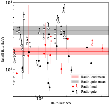
(a)

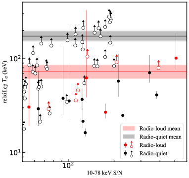
(b)

Figure 2: Similar to Fig. 1 but with $E_{\rm cut}$ (left) and $T_{\rm e}$ (right) derived from $relxill$ and $relxillcp$, respectively.

4.1 Notes on sources with extraordinarily high $E_{cut}$ lower limits

1. NGC 5506, Sy 1.9, $E_{\rm cut}$ $>$ 424 keV ($pexrav$, this work, hereafter the same for the rest 9 sources). Consistently, Matt et al. (2015) reported an $E_{\rm cut}$ = $720_{-190}^{+130}$ keV and a 3$\sigma$ lower limit of 350 keV; Sun et al. (2018) reported an $E_{\rm cut}$ = $500_{-240}^{+100}$ keV; Panagiotou & Walter (2020) reported a 1$\sigma$ lower limit of 8400 keV. The only exception came from Baloković et al. (2020), which reported an $E_{\rm cut}$ = 110 $\pm$ 10 keV with contemporaneous Swift/BAT data. Baloković et al. (2020) claimed in its appendix that the BAT spectrum shows a much smaller cutoff than the NuSTAR one. $E_{\rm cut}$ variation and background subtraction may have played a role.

2. NGC 1566, Sy 1.5, $E_{\rm cut}$ $>$ 434 keV. Akylas & Georgantopoulos (2021) reported an $E_{\rm cut}$ = $336_{-140}^{+646}$ keV, while Parker et al. (2019) reported an incompatible result of $E_{\rm cut}$ = $167\pm 3$ keV. A possible reason is that Parker et al. (2019) used quasi-simultaneous XMM-Newton data, which has a photon index $\Gamma_{\rm pn}\sim 1.43$, quite different from our result ($\Gamma\sim 1.84$). Besides, the reflection fraction $R_{relxill}$ is $\sim$ 0.09, smaller than that in this work ($R_{relxill}$ $\sim$ 0.25). The data are actually barely simultaneous, considering a start time offset of $\sim$ 10 ks and the fact that NuSTAR exposure is 57 ks while PN exposure is 100 ks. Meanwhile, the inter-instrument calibration issue and the pile-up effect in PN data may also have played a part here.

3. NGC 5273, Sy 1.5, $E_{\rm cut}$ $>$ 467 keV. Panagiotou & Walter (2020) reported a 1$\sigma$ lower limit of 1967 keV. Meanwhile, both Panagiotou & Walter (2020) and this work get $\Gamma\sim$ 1.9. Pahari et al. (2017) reported an $E_{\rm cut}$ = $143_{-40}^{+96}$ keV and $\Gamma\sim 1.8$. Note Pahari et al. (2017) employed the quasi-simultaneous Swift-XRT data (6.5 ks XRT exposure, while 21 ks of NuSTAR ) and adopted a quite complex model, which may explain the discrepancy. Akylas & Georgantopoulos (2021) reported an $E_{\rm cut}$ = $115_{-37}^{+95}$ keV, $\Gamma\sim 1.6$ and $R_{pexmon}\sim 0.74$. The reason behind the discrepancy between Akylas & Georgantopoulos (2021) and our result (both fitting only NuSTAR spectra) remains unclear and we can not reproduce their result following the same process with the same model of them (the same for NGC 3516 and Ark 120 below).

4. NGC 3516, Sy 1.2, $E_{\rm cut}$ $>$ 476 keV. Panagiotou & Walter (2020) reported a 1$\sigma$ lower limit of 4940 keV. Akylas & Georgantopoulos (2021) reported an inconsistent $E_{\rm cut}$ = $89_{-48}^{+24}$ keV and a $R_{pexmon}\sim 1.29$.

5. WKK 1263 (IGR J12415-5750), Sy 1.5, $E_{\rm cut}$ $>$ 530 keV. Kamraj et al. (2018), Panagiotou & Walter (2020) and Akylas & Georgantopoulos (2021) reported lower limits of 224 keV, 1826 keV and 282 keV respectively, and all three works derive $\Gamma$ $\sim$ 1.8, similar to our results. Molina et al. (2019) reported an $E_{\rm cut}$ = $123_{-47}^{+54}$ keV, $\Gamma\sim 1.6$ and a similar $R_{pexrav}<0.23$. The involvement of the quasi-simultaneous Swift-XRT data (5.7 ks XRT exposure, while 16 ks of NuSTAR ) in Molina et al. (2019) may account for such discrepancy.

6. Mrk 279, Sy 1.5, $E_{\rm cut}$ $>$ 542 keV. Not reported elsewhere.

7. MCG-06-30-015, Sy 1.9, $E_{\rm cut}$ $>$ 707 keV. Panagiotou & Walter (2020) reported a 1$\sigma$ lower limit of 12000 keV.

8. Ark 120, Sy 1, $E_{\rm cut}$ $>$ 744 keV. Consistently, Panagiotou & Walter (2020) reported a 1$\sigma$ lower limit of 1631 keV; Hinkle & Mushotzky (2021) reported an $E_{\rm cut}$ = $506_{-200}^{+814}$ keV; Nandi et al. (2021) reported an $T_{\rm e}$ = $222_{-107}^{+105}$ keV; Marinucci et al. (2019) reported an $T_{\rm e}$ = $155_{-55}^{+350}$ keV. The only statistically inconsistent result comes from Akylas & Georgantopoulos (2021) which reported an $E_{\rm cut}$ = $233_{-67}^{+147}$ keV.

9. NGC 4593, Sy 1, $E_{\rm cut}$ $>$ 800 keV. Zhang et al. (2018), Panagiotou & Walter (2020) and Akylas & Georgantopoulos (2021) reported an $E_{\rm cut}$ lower limits of 450 keV, 6972 keV and 220 keV respectively. Ursini et al. (2016) reported an $E_{\rm cut}$ = $470_{-150}^{+430}$ keV.

10. NGC 4051, Sy 1.5, $E_{\rm cut}$ $>$ 800 keV. Akylas & Georgantopoulos (2021) reported an $E_{\rm cut}$ lower limits of 846 keV.

In general, our large lower limits to $E_{\rm cut}$ are consistent with most of those from the literature. Discrepancies do exist in some sources, mostly due to the inclusion of the data from other missions in some literature studies. In this work, the $E_{\rm cut}$/$T_{\rm e}$ of the radio-loud and radio-quiet sample are measured with solely NuSTAR spectra, uniformly processed and analyzed. We therefore anticipate the comparison between two samples in this work is unbiased, though the specific measurement of $E_{\rm cut}$ in individual sources could be altered if including quasi-simultaneous observations or using a more complex model. The spectra and the best-fit data-to-model residuals of these ten sources (as shown in the Appendix) have been visually examined and no clear systematical residuals could be identified.

4.2 The reliability of large $E_{\rm cut}$

The large $E_{\rm cut}$ lower limits reported in this work, and the generally consistent results from literature studies, appear to contradict our intuition as such large $E_{\rm cut}$ lower limits are far beyond the NuSTAR spectral coverage (3–78 keV). For instance, the correcting factor of an 800 keV exponential cutoff to a single power law is only $\approx e^{-0.1}$ (around 10%) at 78 keV , making the measurements of large $E_{\rm cut}$ only possible in a few brightest sources with sufficiently high NuSTAR spectral S/N at high energy end. However, as García et al. (2015) pointed out, the reflection component, which is sensitive to the spectral shape of the hardest coronal radiation, may assist the measurements of high $E_{\rm cut}$ with NuSTAR spectra . Based on the $relxill$ model, they showed that $E_{\rm cut}$ can be constrained at as high as 1 MeV for bright sources. Below we also demonstrate the effect of the reflection component in model $pexrav$ with spectral simulations. Using the NuSTAR spectra of NGC 4051 as input, with $E_{\rm cut}$ set at $10^{6}$ keV and other parameters at the best-fit values, we generate artificial spectra assuming different $R$ in $pexrav$ using $fakeit$. Fitting the artificial spectra following the same process we apply on the real spectra, we successfully constrain the $E_{\rm cut}$ lower limit to be above 800 keV in 0.2%, 23% and 40% of the mock spectra, for $R=$ 0, 1 and 2, respectively. This clearly shows that large $E_{\rm cut}$ can be better constrained in spectra with stronger reflection component.

We also check up other factors which may affect the reliability of the high $E_{\rm cut}$ lower limits. The NuSTAR images have been visually double-checked and confirmed to be normal. Moreover, using the traditional method of background subtraction instead of employing the NUSKYBGD, i.e., extracting the background within a region close to the source, would not alter the main results here.

In Fig. 3 we plot $E_{\rm cut}$ versus the 50–78 keV S/N and $E_{\rm cut}$ versus the 50–78 keV background fraction for our sample. Although in a considerable fraction (32%) of our sources, their NuSTAR spectra appear background dominated at $>$ 50 keV (i.e., with 50–78 keV background fraction $>$ 50%), in all but one sources the net 50–78 keV (FPMA) S/N are $>$ 3. This indicates our spectral fitting results are unlikely biased by poor spectral quality or high background level at high energies. From Fig. 3 we also see that $E_{cut}$ lower limits increase with 50–78 keV S/N, and decrease with 50–78 keV background fraction. In other words, these high $E_{cut}$ lower limits ($>$ 400 keV) can only be obtained at relatively higher 50–78 keV S/N and lower 50–78 keV background fraction. This confirms these high $E_{cut}$ lower limits are not due to strong background or poor spectral quality at highest energies.

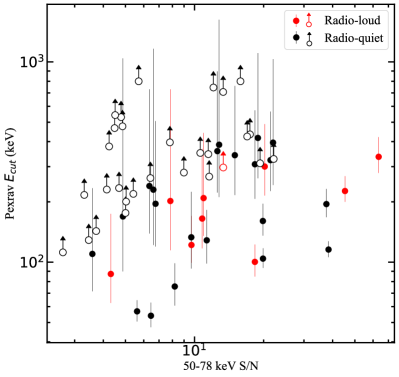
(a)

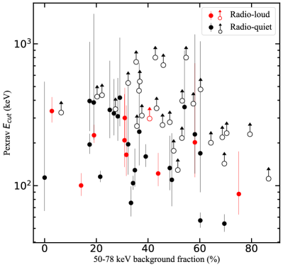
(b)

Figure 3: $pexrav$ $E_{\rm cut}$ versus 50–78 keV (FPMA) S/N and background fraction. The S/N would be elevated by a factor of $\sqrt{2}$ if considering both FPMA an FPMB, but the background fraction would remain unchanged.

Beside, we note complex parameter degeneracy may exist between $E_{\rm cut}$ and other parameters (e.g., Hinkle & Mushotzky, 2021). We hence review the fitting results in individual sources using two parameter contours, among which six sources with $E_{\rm cut}$ lower limits $>$ 400 keV but controversial $E_{\rm cut}$  detections reported in literature are presented in Fig. 4. For these six sources, the degeneracies between $E_{\rm cut}$, $\Gamma$ and $R$ are found to be weak, with a 2$\sigma$ $E_{\rm cut}$ lower limit $\sim$ 300 keV obtained even using two parameter confidence contours. In addition we also demonstrate how the low $E_{\rm cut}$ detections reported in literature (see §4.1) deteriorate the spectral fitting in the lower panel for each source of Fig. 4. We conclude our results are robust in the sense of fitting statistics. See §4.3 and §4.4 for further discussion on the effect of parameter degeneracy.

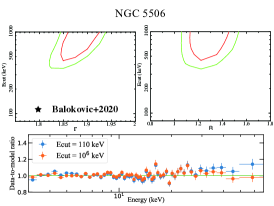
(a)

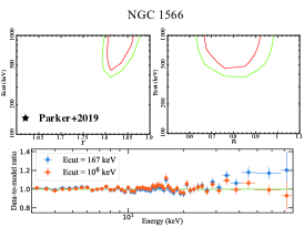
(b)

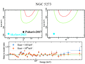
(c)

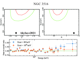
(d)

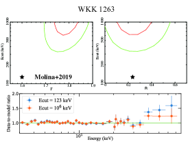
(e)

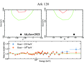
(f)

Figure 4: Upper panel: the $\Gamma$ – $E_{\rm cut}$ and $R$ – $E_{\rm cut}$ contours (with confidence levels of 1$\sigma$ and 2$\sigma$ plotted, corresponding to $\Delta\chi^{2}=$ 2.3 and 4.21) of six sources with $E_{\rm cut}$ lower limits $>$ 400 keV but with statistically inconsistent low $E_{\rm cut}$ detections reported in literature. We mark the reported small $E_{\rm cut}$ detections, together with powerlaw index $\Gamma$ and $pexrav$/$pexmon$ reflection parameter $R$ (when available) from literature for comparison. Lower panel: the data-to-model ratios of the best-fitting results with $E_{\rm cut}$ fixed at $10^{6}$ keV and at the reported low values from literature (see §4.1) respectively. For better illustration, the data have been rebinned and only the FPMA spectra are plotted.

Finally, the three models we adopted in this work ensure the main results are model independent. As shown in Tab. 2, the $E_{\rm cut}$ measurements of $pexrav$ generally agree with those of $relxill$, particularly for those sources with large $E_{\rm cut}$ lower limits. As for the Comptonization model, $T_{\rm e}$ is often harder to be constrained (more lower limits, less detections) than the $E_{\rm cut}$, and the lower limits to $T_{\rm e}$ are smaller than 1/3 $E_{\rm cut}$ (Petrucci et al., 2001) in some sources. This is likely because the e-folded power law produces a smoother break (thus extending to lower energy range and could be better constrained in case of large $T_{\rm e}$/$E_{\rm cut}$ ) than Comptonization models (Zdziarski et al., 2003; Fabian et al., 2015). However, the overall results from the three models are accordant, i.e., sources with extremely large $E_{\rm cut}$ lower limits do have relatively high $T_{\rm e}$, especially compared with radio-loud sources (see next section). We hence rule out the possibility that the large $E_{\rm cut}$/$T_{\rm e}$ lower limits we obtained are due to unknown faults of certain models.

4.3 The difference between radio-quiet and loud samples

We have shown that our radio-quiet sample has considerably larger mean $T_{\rm e}$/$E_{\rm cut}$ compared with the radio-loud one. To explore the statistical reliability of the difference, we need to explore various biases behind the $E_{\rm cut}$ measurements which might be significant here. The first is the complex degeneracies between the spectral parameters; although we have shown above an example that the degeneracies appear weak in individual sources, we need to quantitatively explore whether such effects could be responsible for the different $E_{\rm cut}$ between two samples. The second fact is the radio-loud sample is known to have prominently flatter spectra and weaker reflection component than the radio-quiet one (see Fig. 6); while flatter spectra imply relatively more photons at high energy end, facilitating the $E_{\rm cut}$ measurement, the weaker reflection could contrarily make it hard to constrain high $E_{\rm cut}$. The measurements of $E_{\rm cut}$ also rely on the spectral S/N as shown in Fig. 1, the effect of which could vary from source to source. Last but might be most important, the Kaplan-Meier estimator itself can be sensitive to the size of the sample, the fraction of the censored data (lower limits), and the extremely large lower limits. As shown in Fig. 1 and especially in the right panel of Fig. 2, the mean values, even calculated in the logarithm space, are severely biased towards those large lower limits.

To address the overall complicated biases, we employ the $fakeit$ within XSPEC to create simulated spectra for each source using the best-fit results from $pexrav$ but manually assigning a set of $E_{\rm cut}$ as input. We repeat the spectral fitting to the mock spectra and then the measurement of mean $E_{\rm cut}$ for the mock samples with the Kaplan-Meier estimator, to examine whether our overall procedures could well recover the input $E_{\rm cut}$ or produce artificial different mean $E_{\rm cut}$ between two samples. As shown in Fig. 5, while the simulations do could recover the input $E_{\rm cut}$ in case of low $E_{\rm cut}$ values, high input $E_{\rm cut}$ values (400 keV and above) are clearly underestimated, because the limited bandwidth of NuSTAR, and because we have manually fixed the larger $E_{\rm cut}$ lower limit to 800 keV. Since a considerably fraction of radio-quiet sources have rather large intrinsic $E_{\rm cut}$ while none of radio-loud sources does, this indicates we may have underestimated the mean $E_{\rm cut}$ for our real radio-quiet sample, further strengthening the difference between two samples we have observed. However, no statistical difference is found between the mock radio-loud and radio-quiet samples. We therefore conclude the biases aforementioned put together are unable to account for the difference in the $E_{\rm cut}$ distribution between two samples.

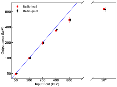
(a)

Figure 5: Output mean $E_{\rm cut}$ (in unit of keV) from the mock samples. Note the output mean $E_{\rm cut}$ saturates at $\sim$ 800 keV, partially because we manually set larger $E_{\rm cut}$ lower limits yielded from spectral fitting to 800 keV.

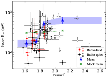
(a)

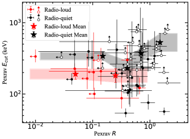
(b)

Figure 6: Upper: $E_{\rm cut}$ versus $\Gamma$. We over-plot the mean $E_{\rm cut}$ within several bins of $\Gamma$ for all sources as we find no difference in the mean $E_{\rm cut}$ between radio-quiet and radio-loud sources at given $\Gamma$. Meanwhile, the output mean $E_{\rm cut}$ versus output $\Gamma$ derived from the mock spectra of the sample (with input $E_{\rm cut}$ = 400 keV) is over-plotted as green crosses. Lower: $E_{\rm cut}$ versus $R$.

The larger average $E_{\rm cut}$ in radio-quiet sources is however surprising, as we would anticipate larger observed $E_{\rm cut}$ in the radio-loud sample due to potential jet contamination (Madsen et al., 2015b) or the stronger Doppler boosting of an outflowing corona in radio AGNs (e.g. Beloborodov, 1999; Liu et al., 2014; Kang et al., 2020), even if two populations have the same intrinsic coronal temperature. The key underlying reason might be the different $\Gamma$ distribution of the two samples. In Fig. 6 we plot $E_{\rm cut}$ versus $\Gamma$ and the reflection strength $R$ from $pexrav$ for the two samples. We find that $E_{\rm cut}$ is positively correlated with $\Gamma$ and those large $E_{\rm cut}$ lower limits are mainly detected in sources with steep spectra. Besides, we find no difference in $E_{\rm cut}$ between two populations at comparable $\Gamma$. Therefore, the difference in $E_{\rm cut}$ between two populations could dominantly be attributed to the fact that $E_{\rm cut}$ correlates with photon index $\Gamma$ while the radio-loud sample is dominated by sources with flat spectra. Meanwhile, $E_{\rm cut}$ exhibits no clear correlation with $R$, while RQ AGNs do show larger $E_{\rm cut}$ compared with RL ones at given $R$, which could be attributed to the effect of $\Gamma$. We note that Kang et al. (2020) found the $E_{\rm cut}$ distribution of their radio-loud sample is indistinguishable from that of a radio-quiet sample from Rani et al. (2019). This is likely because the sample of Rani et al. (2019) is incomplete, which only collected from literature sources with well-constrained $E_{\rm cut}$ and most lower limits were excluded. In fact, if we drop lower limits from our samples in this work, we would find no difference either in mean $E_{\rm cut}$ between two populations. Meanwhile, Gilli et al. (2007) has shown an average $E_{\rm cut}$ of above 300 keV can saturate the X-ray Background at 100 keV. The fact that large $E_{\rm cut}$ mainly exist in steeper spectra also renders our large mean value of $E_{\rm cut}$ in radio-quiet AGNs compatible with Gilli et al. (2007), as sources with steep X-ray spectra make little contribution to the high energy X-ray background even with a large $E_{\rm cut}$.

4.4 The underlying mechanisms

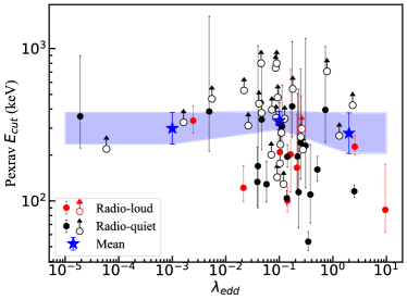
(a)

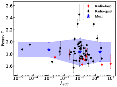
(b)

Figure 7: $E_{\rm cut}$ – $\lambda_{\rm edd}$ and $\Gamma$ – $\lambda_{\rm edd}$ for our samples. $\lambda_{edd}$ is derived using the black hole mass from literature and up-scaled BAT 14–195 keV luminosity (see Tab. 1).

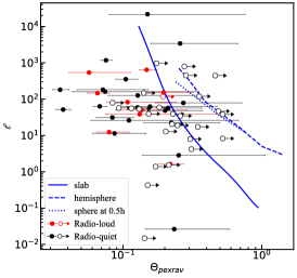
(a)

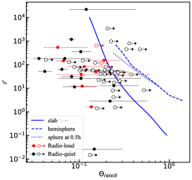
(b)

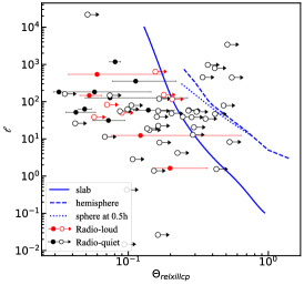
(c)

Figure 8: The compactness–temperature ($l$–$\Theta$) diagrams, with $\Theta$ derived from three spectral models.

Tentative positive correlation between $E_{\rm cut}$ and $\Gamma$ has been reported in other studies with NuSTAR (e.g. Kamraj et al., 2018; Molina et al., 2019; Hinkle & Mushotzky, 2021), and previously with BeppoSAX data (e.g. Petrucci et al., 2001), however not as pronounced as we have found, likely because of smaller sample size or the domination by poorly constrained lower limits. For instance, the sample in Kamraj et al. (2018) consists of 46 sources, whereas $E_{\rm cut}$ can be well constrained in only two of them. The samples in Molina et al. (2019) and Hinkle & Mushotzky (2021) consist of 18 and 33 sources respectively, considerably smaller than the one presented in this work; meanwhile, the inclusion of XRT and XMM-Newton data in those two works may have disturbed the measurements of $E_{\rm cut}$ and $\Gamma$ as already discussed above.

The tentative $E_{\rm cut}$ – $\Gamma$ correlation reported in literature had often been attributed to the parameter degeneracy between $E_{\rm cut}$ and $\Gamma$. In this work, the correlation between $E_{\rm cut}$ and $\Gamma$ is rather strong, and $\Gamma$ is well constrained thanks to the high-quality NuSTAR spectra. We thus expect the effect of such degeneracy to be insignificant. We perform simulations to quantify such effect in our sample. Utilizing an $E_{\rm cut}$ =400 keV as input and other best-fit spectral parameters from $pexrav$, we simulate mock spectra for each source. We then examine the correlation between the output $E_{\rm cut}$ and output $\Gamma$ for the mock sample. As shown Fig. 6, while the parameter degeneracy does yield a weak artificial correlation between the output $E_{\rm cut}$ and $\Gamma$, it is much weaker and negligible compared with the observed one.

The positive correlation between $E_{\rm cut}$ and $\Gamma$ found in this work indicates sources with steeper X-ray spectra tend to hold hotter coronae. Subsequently, to produce the steeper spectra, the hotter coronae need to have lower opacity. The negative link between coronal temperature and opacity could partly be attributed to the fact that the cooling is more efficient in coronae with higher opacity, i.e., sustainable hotter coronae are only possible with lower opacity. However, while lower opacity could lead to steeper spectra, higher temperature alters the spectral slope towards an opposite direction. While it is yet unclear what drives the positive $E_{\rm cut}$ – $\Gamma$ correlation reported in this work, it is intriguing to compare it with how $E_{\rm cut}$ varies with $\Gamma$ in individual AGNs. $E_{\rm cut}$ variabilities detected in several individual AGNs show a common trend that when an individual source brightens in X-ray flux, its power law spectrum gets softer and $E_{\rm cut}$ increases, also revealing a positive $E_{\rm cut}$ – $\Gamma$ correlation (hotter-when-softer/brighter, e.g. Zhang et al., 2018; Kang et al., 2021). However, the similarity between the two types of positive $E_{\rm cut}$ – $\Gamma$ correlation (intrinsic: in individual AGNs, versus global: in a large sample of AGNs) does not necessarily imply common underlying mechanisms. This is because, while the intrinsic $E_{\rm cut}$ – $\Gamma$ correlation, which could be accompanied with dynamical/geometrical changes of the coronae such as inflation/contraction (Wu et al., 2020), reflects variations in the inner most region of individual AGNs, the global $E_{\rm cut}$ – $\Gamma$ correlation we find in a sample of AGNs shall mainly reflect the differences in their physical properties, including SMBH mass, accretion rate and other unknown parameters. Kang et al. (2021) also found a tentative trend that $E_{\rm cut}$ reversely decreases with $\Gamma$ at $\Gamma$ $>$ 2.05 in one individual source, yielding a $\Lambda$ shape in the $E_{\rm cut}$ – $\Gamma$ diagram. Such trend however is not seen in the global $E_{\rm cut}$ – $\Gamma$ relation.

The positive global $E_{\rm cut}$ – $\Gamma$ correlation also implies a potential positive correlation between $E_{\rm cut}$ and Eddington ratio $\lambda_{edd}$, as sources with higher accretion rate tend to have steeper spectra (e.g. Shemmer et al., 2006; Risaliti et al., 2009; Yang et al., 2015). However, we find no significant correlation between $\lambda_{edd}$ and $\Gamma$, or between $\lambda_{edd}$ and $E_{\rm cut}$ in our sample (see Fig. 7), consistent with the results of Molina et al. (2019), Hinkle & Mushotzky (2021) and Kamraj et al. (2022). This is likely because the uncertainties in the measurements of $\lambda_{edd}$ are large, or the $E_{\rm cut}$ – $\Gamma$ correlation we find is not driven by Eddington ratio. However, our results disagree with Ricci et al. (2018), which claimed a negative correlation between $E_{\rm cut}$ and $\lambda_{edd}$ based on SWIFT BAT spectra. But note a dominant fraction (144 out of 212) of the $E_{\rm cut}$ measurements reported in Ricci et al. (2018) are lower limits.

We note a couple of individual local sources with high Eddington ratios ( $>$ 1) have been reported with NuSTAR spectra to have low $E_{\rm cut}$/$T_{\rm e}$ in literature (e.g., Ark 564, IRAS 04416+1215, Kara et al., 2017; Tortosa et al., 2022), seeming to suggest lower coronal temperature at higher Eddington ratio. While the NuSTAR spectral quality of Ark 564 is rather high (10–78 keV FPMA S/N = 88), it is not in the 105-month SWIFT/BAT catalog, thus not included in this work. The NuSTAR spectral quality of IRAS 04416+1215 (with 10–78 keV S/N of 10) is much poorer compared with the sample presented in this work, and our independent fitting to its NuSTAR spectra alone could only yield poorly constrained lower limits to its $E_{\rm cut}$ or $T_{\rm e}$. Utilizing XMM-Newton and NuSTAR data, low $E_{\rm cut}$/$T_{\rm e}$ is also detected in a high-redshift source with Eddington ratio $>$ 1 (PG 1247+267, Lanzuisi et al., 2016). However, its NuSTAR spectra also have poor S/N ($\sim$ 20 in the rest frame 10–78 keV). Meanwhile, simply collecting positive detections of $E_{\rm cut}$/$T_{\rm e}$ from literature could suffer significant publication bias.

We finally plot the samples on the well-known compactness–temperature ($l$–$\Theta$) diagram. Fabian et al. (2015) has shown that, the AGN coronae locate near the boundary of the forbidden region in the $l$–$\Theta$ diagram, suggesting the coronal temperature is governed and limited by runaway pair production. Following Fabian et al. (2015), we calculate the compactness, $l=4\pi(m_{p}/m_{e})(r_{g}/r)(L/L_{\rm edd})$, and dimensionless temperature, $\Theta=kT_{e}/m_{e}c^{2}$. We assume a $r=10$ $r_{g}$, adopt the unabsorbed 0.1–200 keV primary continuum luminosity extrapolated by the best-fit $pexrav$ model to NuSTAR spectra (listed in Table 1), and calculate $L_{\rm edd}$ using the SMBH mass in Table 1. For $pexrav$ and $relxill$, the $T_{\rm e}$ is approximated by $E_{\rm cut}$/3 (Petrucci et al., 2001), while for $relxillcp$ the measured $T_{\rm e}$ is directly used. The $l$–$\Theta$ diagrams of the three models are shown in Fig. 8, with the boundaries of runaway pair production of the three geometries (Stern et al., 1995; Svensson, 1996) over-plotted. Apparently, the sources in this work have a wider $\Theta$ range compared with that of Fabian et al. (2015), likely because of the large sample size of this work. On the one hand, there are many sources lying clearly to the left of the slab pair line, particularly sources in the upper left corner in the $l$–$\Theta$ diagram. They appear to support the existence of hybrid plasma in the coronae as hybrid plasma would shift the pair line to the left and the shift is more prominent in the top of the line (see Fig. 6 in Fabian et al., 2017). On the other hand, both the directly measured and conservatively estimated $T_{\rm e}$ (1/3 $E_{\rm cut}$ here, while 1/2 in Fabian et al. 2015) of a considerable fraction of sources lie beyond (to the right of) the slab pair line, consistent with Kamraj et al. (2022), favoring the sphere or hemisphere geometry. Considering the $E_{\rm cut}$ – $\Gamma$ relation shown above, it is implied that the coronal geometry might be spectral slope dependent, i.e., flatter shape for harder spectra, and rounder for softer spectra. Furthermore there are several sources with lower limits of $\Theta$ lying even beyond the boundaries of all three geometries, which suggests their coronae could be more extended than 10 $r_{g}$ we have assumed.

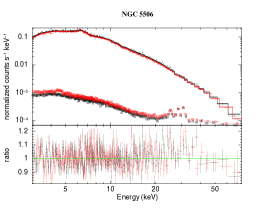
(a)

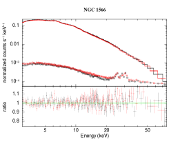
(b)

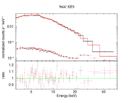
(c)

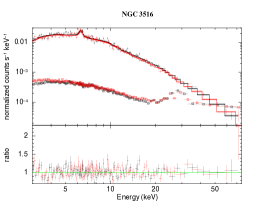
(d)

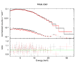
(e)

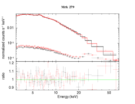
(f)

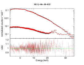
(g)

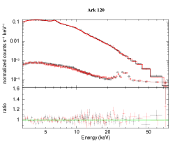
(h)

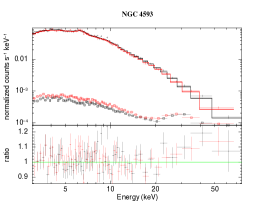
(i)

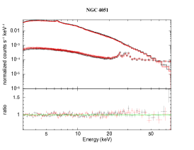
(j)

Figure 9: NuSTAR source and background spectra (estimated by NUSKYBGD), the best-fit models and the data-to-model residual ($pexrav$) ratios of the 10 sources with large $E_{\rm cut}$ lower limits ($>$ 400 keV), ordered from low to high by the $E_{\rm cut}$ lower limit). Note in only a few of them, e.g., NGC 3516 and NGC 4051, the spectra appear background dominated (i.e., the background fluxes larger than source fluxes) at above 50 keV. Spectra from both FPMA (black) and FPMB (red) modules are given and further rebinned for visualization purposes.

References

- Akylas & Georgantopoulos (2021) Akylas, A., & Georgantopoulos, I. 2021, arXiv e-prints, arXiv:2108.11337. https://arxiv.org/abs/2108.11337
- Alston et al. (2020) Alston, W. N., Fabian, A. C., Kara, E., et al. 2020, Nature Astronomy, 2, doi: 10.1038/s41550-019-1002-x
- Anders & Grevesse (1989) Anders, E., & Grevesse, N. 1989, Geochimica et Cosmochimica Acta, 53, 197 , doi: 10.1016/0016-7037(89)90286-X
- Arnaud (1996) Arnaud, K. A. 1996, in Astronomical Society of the Pacific Conference Series, Vol. 101, Astronomical Data Analysis Software and Systems V, ed. G. H. Jacoby & J. Barnes, 17
- Ballantyne et al. (2014) Ballantyne, D. R., Bollenbacher, J. M., Brenneman, L. W., et al. 2014, The Astrophysical Journal, 794, 62, doi: 10.1088/0004-637x/794/1/62
- Baloković et al. (2020) Baloković, M., Harrison, F. A., Madejski, G., et al. 2020, ApJ, 905, 41, doi: 10.3847/1538-4357/abc342
- Beloborodov (1999) Beloborodov, A. M. 1999, ApJ, 510, L123, doi: 10.1086/311810
- Blinov et al. (2021) Blinov, D., Jorstad, S. G., Larionov, V. M., et al. 2021, MNRAS, 505, 4616, doi: 10.1093/mnras/stab1484
- Cappellari et al. (2009) Cappellari, M., Neumayer, N., Reunanen, J., et al. 2009, MNRAS, 394, 660, doi: 10.1111/j.1365-2966.2008.14377.x
- Cappi et al. (2016) Cappi, M., De Marco, B., Ponti, G., et al. 2016, A&A, 592, A27, doi: 10.1051/0004-6361/201628464
- Fabian et al. (2017) Fabian, A. C., Lohfink, A., Belmont, R., Malzac, J., & Coppi, P. 2017, MNRAS, 467, 2566, doi: 10.1093/mnras/stx221
- Fabian et al. (2015) Fabian, A. C., Lohfink, A., Kara, E., et al. 2015, MNRAS, 451, 4375, doi: 10.1093/mnras/stv1218
- Fabian et al. (2009) Fabian, A. C., Zoghbi, A., Ross, R. R., et al. 2009, Nature, 459, 540, doi: 10.1038/nature08007
- Feigelson & Nelson (1985) Feigelson, E. D., & Nelson, P. I. 1985, ApJ, 293, 192, doi: 10.1086/163225
- García et al. (2014) García, J., Dauser, T., Lohfink, A., et al. 2014, ApJ, 782, 76, doi: 10.1088/0004-637X/782/2/76
- García et al. (2015) García, J. A., Dauser, T., Steiner, J. F., et al. 2015, ApJ, 808, L37, doi: 10.1088/2041-8205/808/2/L37
- Gilli et al. (2007) Gilli, R., Comastri, A., & Hasinger, G. 2007, A&A, 463, 79, doi: 10.1051/0004-6361:20066334
- Haardt & Maraschi (1991) Haardt, F., & Maraschi, L. 1991, ApJ, 380, L51, doi: 10.1086/186171
- Haardt & Maraschi (1993) —. 1993, ApJ, 413, 507, doi: 10.1086/173020
- Harrison et al. (2013) Harrison, F. A., Craig, W. W., Christensen, F. E., et al. 2013, The Astrophysical Journal, 770, 103, doi: 10.1088/0004-637x/770/2/103
- Hinkle & Mushotzky (2021) Hinkle, J. T., & Mushotzky, R. 2021, MNRAS, 506, 4960, doi: 10.1093/mnras/stab1976
- Kamraj et al. (2018) Kamraj, N., Harrison, F. A., Baloković, M., Lohfink, A., & Brightman, M. 2018, The Astrophysical Journal, 866, 124, doi: 10.3847/1538-4357/aadd0d
- Kamraj et al. (2022) Kamraj, N., Brightman, M., Harrison, F. A., et al. 2022, arXiv e-prints, arXiv:2202.00895. https://arxiv.org/abs/2202.00895
- Kang et al. (2020) Kang, J., Wang, J., & Kang, W. 2020, ApJ, 901, 111, doi: 10.3847/1538-4357/abadf5
- Kang et al. (2021) Kang, J.-L., Wang, J.-X., & Kang, W.-Y. 2021, MNRAS, 502, 80, doi: 10.1093/mnras/stab039
- Kara et al. (2017) Kara, E., García, J. A., Lohfink, A., et al. 2017, MNRAS, 468, 3489, doi: 10.1093/mnras/stx792
- Keek & Ballantyne (2016) Keek, L., & Ballantyne, D. R. 2016, MNRAS, 456, 2722, doi: 10.1093/mnras/stv2882
- Koss et al. (2017) Koss, M., Trakhtenbrot, B., Ricci, C., et al. 2017, ApJ, 850, 74, doi: 10.3847/1538-4357/aa8ec9
- Lanzuisi et al. (2016) Lanzuisi, G., Perna, M., Comastri, A., et al. 2016, A&A, 590, A77, doi: 10.1051/0004-6361/201628325
- Lewis & Eracleous (2006) Lewis, K. T., & Eracleous, M. 2006, ApJ, 642, 711, doi: 10.1086/501419
- Liu et al. (2014) Liu, T., Wang, J.-X., Yang, H., Zhu, F.-F., & Zhou, Y.-Y. 2014, ApJ, 783, 106, doi: 10.1088/0004-637X/783/2/106
- Madsen et al. (2020) Madsen, K. K., Grefenstette, B. W., Pike, S., et al. 2020, arXiv e-prints, arXiv:2005.00569. https://arxiv.org/abs/2005.00569
- Madsen et al. (2015a) Madsen, K. K., Harrison, F. A., Markwardt, C. B., et al. 2015a, ApJS, 220, 8, doi: 10.1088/0067-0049/220/1/8
- Madsen et al. (2015b) Madsen, K. K., Fürst, F., Walton, D. J., et al. 2015b, ApJ, 812, 14, doi: 10.1088/0004-637X/812/1/14