On Semialgebraic Range Reporting

Abstract

Semialgebraic range searching, arguably the most general version of range searching, is a fundamental problem in computational geometry. In the problem, we are to preprocess a set of points in $\mathbb{R}^{D}$ such that the subset of points inside a semialgebraic region described by a constant number of polynomial inequalities of degree $\Delta$ can be found efficiently.

Relatively recently, several major advances were made on this problem. Using algebraic techniques, “near-linear space” data structures [6, 18] with almost optimal query time of $Q(n)=O(n^{1-1/D+o(1)})$ were obtained. For “fast query” data structures (i.e., when $Q(n)=n^{o(1)}$), it was conjectured that a similar improvement is possible, i.e., it is possible to achieve space $S(n)=O(n^{D+o(1)})$. The conjecture was refuted very recently by Afshani and Cheng [3]. In the plane, i.e., $D=2$, they proved that $S(n)=\Omega(n^{\Delta+1-o(1)}/Q(n)^{(\Delta+3)\Delta/2})$ which shows $\Omega(n^{\Delta+1-o(1)})$ space is needed for $Q(n)=n^{o(1)}$. While this refutes the conjecture, it still leaves a number of unresolved issues: the lower bound only works in 2D and for fast queries, and neither the exponent of $n$ or $Q(n)$ seem to be tight even for $D=2$, as the best known upper bounds have $S(n)=O(n^{\boldsymbol{m}+o(1)}/Q(n)^{(\boldsymbol{m}-1)D/(D-1)})$ where $\boldsymbol{m}=\binom{D+\Delta}{D}-1=\Omega(\Delta^{D})$ is the maximum number of parameters to define a monic degree-$\Delta$ $D$-variate polynomial, for any constant dimension $D$ and degree $\Delta$.

In this paper, we resolve two of the issues: we prove a lower bound in $D$-dimensions, for constant $D$, and show that when the query time is $n^{o(1)}+O(k)$, the space usage is $\Omega(n^{\boldsymbol{m}-o(1)})$, which almost matches the $\tilde{O}(n^{\boldsymbol{m}})$ upper bound and essentially closes the problem for the fast-query case, as far as the exponent of $n$ is considered in the pointer machine model. When considering the exponent of $Q(n)$, we show that the analysis in [3] is tight for $D=2$, by presenting matching upper bounds for uniform random point sets. This shows either the existing upper bounds can be improved or to obtain better lower bounds a new fundamentally different input set needs to be constructed.

1 Introduction

In the classical semialgebraic range searching problem, we are to preprocess a set of $n$ points in $\mathbb{R}^{D}$ such that the subset of points inside a semialgebraic region, described by a constant number of polynomial inequalities of degree $\Delta$ can be found efficiently. Recently, two major advances were made on this problem. First, in 2019, Agarwal et al. [5] showed for polylogarithmic query time, it is possible to build a data structure of size $\tilde{O}(n^{\beta})$ space, where $\beta$ is the number of parameters needed to specify a query polynomial. For example, for $D=2$, a query polynomial is in the form of $\sum_{i+j\leq\Delta}a_{ij}x^{i}y^{j}\leq 0$ where $a_{ij}$’s are specified at the query time, and when $\Delta=4$, $\beta$ can be as large as $14$ (technically, there are 15 coefficients but one coefficient can always be normalized to be 1). In this case, a major conjecture was that if this space bound could be improved to $\tilde{O}(n^{D})$ (e.g., for $\Delta=4$, from $\tilde{O}(n^{14})$ to $\tilde{O}(n^{2})$). Very recently, Afshani and Cheng [3] refuted this conjecture by showing a $\overset{\scriptscriptstyle o}{\Omega}(n^{\Delta+1})$ lower bound. However, there are two major limitations of their lower bound. First, their lower bound only works in $\mathbb{R}^{2}$, while the upper bound in [5] holds for all dimensions. Second, their lower bound only works for queries of form $y-\sum_{i=0}^{\Delta}x^{i}\leq 0$ and thus their lower bound does not give a satisfactory answer to the problem in the general case. For example, for $D=2,\Delta=4$, they show a $\overset{\scriptscriptstyle o}{\Omega}(n^{5})$ lower bound whereas the current best upper bound is $\tilde{O}(n^{14})$. In general, their space lower bound is at most $\overset{\scriptscriptstyle o}{\Omega}(n^{\Delta+1})$ while the upper bound of [5] can be $\tilde{O}(n^{\Theta(\Delta^{2})})$, which leaves an unsolved wide gap, even for $D=2$. Another problem brought by [5] is the space-time tradeoff. When restricted to queries of the form $y-\sum_{i=0}^{\Delta}x^{i}\leq 0$, the current upper bound tradeoff is $S(n)=\tilde{O}(n^{\Delta+1}/Q(n)^{2\Delta})$ [18, 5] while the lower bound in [3] is $S(n)=\overset{\scriptscriptstyle o}{\Omega}(n^{\Delta+1}/Q(n)^{(\Delta+3)\Delta/2})$. Even for $\Delta=2$, we observe a discrepancy between an $S(n)=\tilde{O}(n^{3}/Q(n)^{4})$ upper and an $S(n)=\overset{\scriptscriptstyle o}{\Omega}(n^{3}/Q(n)^{5})$ lower bound.

Here, we make progress in both lower and upper bound directions. We give a general lower bound in $D$ dimensions that is tight for all possible values of $\beta$. Our lower bound attains the maximum possible $\beta$ value $\boldsymbol{m}_{D,\Delta}=\binom{D+\Delta}{D}-1$, e.g., $\overset{\scriptscriptstyle o}{\Omega}(n^{14})$ for $D=2,\Delta=4$. Thus, our lower bounds almost completely settle the general case of the problem for the fast-query case, as far as the exponent of $n$ is concerned. This improvement is quite non-trivial and requires significant new insights that are not avaiable in [3]. For the upper bound, we present a matching space-time tradeoff for the two problems studied in [3] for uniform random point sets. This shows their lower bound analysis is tight. Since for most range searching problems, a uniform random input instance is the hardest one, our results show that current upper bound based on the classical method might not be optimal. We develop a set of new ideas for our results which we believe are important for further investigation of this problem.

1.1 Background

In range searching, the input is a set of points in $\mathbb{R}^{D}$ for a fixed constant $D$. The goal is to build a structure such that for a query range, we can report or find the points in the range efficiently. This is a fundamental problem in computational geometry with many practical uses in e.g., databases and GIS systems. For more information, see surveys by Agarwal [14] or Matoušek [17]. We focus on a fundamental case of the problem where the ranges are semialgebraic sets of constant complexity which are defined by intersection/union/complementation of $O(1)$ polynomial inequalities of constant degree at most $\Delta$ in $\mathbb{R}^{D}$.

The study of this problem dates back to at least 35 years ago [19]. A linear space and $O(n^{1-1/D+o(1)})$ query time structure is given by Agarwal, Matoušek, and Sharir [6], due to the recent “polynomial method” breakthrough [15]. However, it is not entirely clear what happens to the “fast-query” case: if we insist on polylogarithmic query time, what is the smallest possible space usage? Early on, some believed that the number of parameters plays an important role and thus $\tilde{O}(n^{\beta})$ space could be a reasonable conjecture [17], but such a data structure was not found until 2019 [5]. However, after the “polynomial method” revolution, and specifically after the breakthrough result of Agarwal, Matoušek and Sharir [6], it could also be reasonably conjectured that $\tilde{O}(n^{D})$ could also be the right bound. However, this was refuted recently by Afshani and Cheng [3] who showed that in 2D, and for polynomials for the form $y-\sum_{i=0}^{\Delta}x^{i}\leq 0$, there exists an $\overset{\scriptscriptstyle o}{\Omega}(n^{\Delta+1})$ space lower bound for data structures with query time $\overset{\scriptscriptstyle o}{O}(1)$. However, this lower bound does not go far enough, even in 2D, where a semialgebraic range can be specified by bivariate monic polynomial inequalities of form $\sum_{i,j:i+j\leq\Delta}a_{ij}x^{i}y^{j}\leq 0$ with $a_{\Delta 0}=-1$. In this case, $\beta$ can be as large as $\boldsymbol{m}_{2,\Delta}=\binom{\Delta+2}{2}-1=\Theta(\Delta^{2})$, and much larger than $\Delta+1$ even for moderate $\Delta$ (e.g., for $\Delta=4$, “5” versus “14”, for $\Delta=5$, “6” versus “20” and so on). Another main weakness is that their lower bound is only in 2D, but the upper bound [5] works in arbitrary dimensions.

The correct upper bound tradeoff seems to be even more mysterious. Typically, the tradeoff is obtained by combining the linear space and the polylogarithmic query time solutions. For simplex range searching (i.e., when $\Delta=1$), the tradeoff is $S(n)=\tilde{O}(n^{D}/Q(n)^{D})$ [16], which is a natural looking bound and it is also known to be optimal. The tradeoff bound becomes very mysterious for semialgebraic range searching. For example, for $D=2$ and when restricted to queries of the form $y-\sum_{i=0}^{\Delta}x^{i}\leq 0$, combining the existing solutions yields the bound $S(n)=\tilde{O}(n^{\Delta+1}/Q(n)^{2\Delta})$ whereas the known lower bound [3] is $S(n)=\overset{\scriptscriptstyle o}{\Omega}(n^{\Delta+1}/Q(n)^{(\Delta+3)\Delta/2})$. One possible reason for this gap is that the lower bound construction is based on a uniform random point set, while in practice, the input can be pathological. But in general the uniform random point set assumption is not too restrictive for range searching problems. Almost all known lower bounds rely on this assumption: e.g., half-space range searching [9, 7, 8], orthogonal range searching [11, 12, 2], simplex range searching [10, 13, 1].

1.2 Our Results

Our results consist of two parts. First, we study a problem that we call “the general polynomial slab range reporting”. Formally, let $P(X)$ be a monic $D$-variate polynomial of degree at most $\Delta$, a general polynomial slab is defined to be the region between $P(X)=0$ and $P(X)=w$ for some parameter $w$ specified at the query time. Unlike [3], our construction can reach the maximum possible parameter number $\boldsymbol{m}_{D,\Delta}$. For simplicity, we use $\boldsymbol{m}$ instead of $\boldsymbol{m}_{D,\Delta}$ when the context is clear. We give a space-time tradeoff lower bound of $S(n)=\overset{\scriptscriptstyle o}{\Omega}(n^{\boldsymbol{m}}/Q(n)^{\Theta((\Delta^{2}+D\Delta)\boldsymbol{m}}))$, which is (almost) tight when $Q(n)=n^{o(1)}$.

For the second part, we present data structures that match the lower bounds studied in the work by Afshani and Cheng [3]. We show that their lower bounds for 2D polynomial slabs and 2D annuli are tight for uniform random point sets. Our bound shows that current tradeoff given by the classical method of combining extreme solutions [18, 5] might not be tight. We shred some lights on the upper bound tradeoff and develop some ideas which could be used to tackle the problem. Our results are summarized in Table 1.

Table 1: Our Results (marked by ^∗). Our upper bounds are for uniform random point sets.

Query Types	Lower Bound	Upper Bound
General Polynomial Slabs $\left(\boldsymbol{m}=\boldsymbol{m}_{D,\Delta}=\binom{D+\Delta}{D}-1\right)$	$S(n)=\overset{\scriptscriptstyle o}{\Omega}\left(\frac{n^{\boldsymbol{m}}}{Q(n)^{\Theta(\boldsymbol{m})}}\right)^{*}$	$S(n)=\tilde{O}\left(\frac{n^{\boldsymbol{m}}}{Q(n)^{\Theta(\boldsymbol{m})}}\right)$ [18, 5]
When $\boldsymbol{Q(n)=\overset{\scriptscriptstyle o}{O}(1)}$	$\boldsymbol{S(n)=\overset{\scriptscriptstyle o}{\Omega}\left(n^{\boldsymbol{m}}\right)^{*}}$	$\boldsymbol{S(n)=\tilde{O}\left(n^{\boldsymbol{m}}\right)}$ [18, 5]
2D Semialgebraic Sets $\left(\boldsymbol{m}=\boldsymbol{m}_{2,\Delta}=\binom{2+\Delta}{2}-1\right)$	$S(n)=\overset{\scriptscriptstyle o}{\Omega}\left(\frac{n^{\boldsymbol{m}}}{Q(n)^{\boldsymbol{m}+\boldsymbol{m}^{2}(\boldsymbol{m}-1)-1}}\right)^{*}$	$S(n)=\tilde{O}\left(\frac{n^{\boldsymbol{m}}}{Q(n)^{2\boldsymbol{m}-2}}\right)$ [18, 5] $\boldsymbol{S(n)=\tilde{O}\left(\frac{n^{\boldsymbol{m}}}{Q(n)^{3\boldsymbol{m}-4}}\right)^{*}}$
2D Polynomial Slabs	$\boldsymbol{S(n)=\overset{\scriptscriptstyle o}{\Omega}\left(\frac{n^{\Delta+1}}{Q(n)^{(\Delta+3)\Delta/2}}\right)}$ [3]	$S(n)=\tilde{O}\left(\frac{n^{\Delta+1}}{Q(n)^{2\Delta}}\right)$ [18, 5] $\boldsymbol{S(n)=\tilde{O}\left(\frac{n^{\Delta+1}}{Q(n)^{(\Delta+3)\Delta/2}}\right)^{*}}$
2D Annuli	$\boldsymbol{S(n)=\overset{\scriptscriptstyle o}{\Omega}\left(\frac{n^{3}}{Q(n)^{5}}\right)}$ [3]	$S(n)=\tilde{O}\left(\frac{n^{3}}{Q(n)^{4}}\right)$ [18, 5] $\boldsymbol{S(n)=\tilde{O}\left(\frac{n^{3}}{Q(n)^{5}}\right)^{*}}$

1.3 Technical Contributions

Compared to the previous lower bound in [3], we need to wrestle with many complications that stem from the algebraic geometry nature of the problem. In Section 3, we cover them in greater detail, but briefly speaking, the technical heart of the results in [3] is that “two univariate polynomials $P_{1}(x)$ and $P_{2}(x)$ that have sufficiently different leading coefficients, cannot pass close to each other for too long. However, this claim is not true for even bivariate polynomials, since $P_{1}(x,y)$ and $P_{2}(x,y)$ could have infinitely many roots in common and thus we can have $P_{1}(x,y)-P_{2}(x,y)=0$ in an unbounded region of $\mathbb{R}^{2}$. Overcoming this requires significant innovations.

2 Preliminaries

In this section, we introduce some tools we will use in this paper. We will mainly use the lower bound tools used in [3]. For more detailed introduction, we refer the readers to [3].

2.1 A Geometric Lower Bound Framework

We present a lower bound framework in the pointer machine model of computation. It is a streamlined version of the framework by Chazelle [11] and Chazelle and Rosenberg [13]. In essence, this is an encapsulation of the way the framework is used in [3].

In a nutshell, in the pointer machine model, the memory is represented as a directed graph where each node can store one point and it has two pointers to two other nodes. Given a query, starting from a special “root” node, the algorithm explores a subgraph that contains all the input points to report. The size of the explored subgraph is the query time.

Intuitively, for range reporting, to answer a query fast, we need to store its output points close to each other. If each query range contains many points to report and two ranges share very few points, some points must be stored multiple times, thus the total space usage must be big. We present the framework, and refer the readers to the Appendix A for the proof.

theoremrrfw Suppose the $D$-dimensional geometric range reporting problems admit an $S(n)$ space $Q(n)+O(k)$ query time data structure, where $n$ is the input size and $k$ is the output size. Let $\mu^{D}(\cdot)$ denote the $D$-dimensional Lebesgue measure. Assume we can find $m=n^{c}$ ranges $\mathscr{R}_{1},\mathscr{R}_{2},\cdots,\mathscr{R}_{m}$ in a $D$-dimensional cube $\boldsymbol{C}^{D}$ of side length $|l|$ for some constant $c$ such that (i) $\forall i=1,2,\cdots,m,\mu^{D}(\mathscr{R}_{i}\cap\boldsymbol{C}^{D})\geq 4c|l|^{D}Q(n)/n$; and (ii) $\mu^{D}(\mathscr{R}_{i}\cap\mathscr{R}_{j})=O(|l|^{D}/(n2^{\sqrt{\log n}}))$ for all $i\neq j$. Then, we have $S(n)=\overset{\scriptscriptstyle o}{\Omega}(mQ(n))$.

2.2 A Lemma for Polynomials

Given a univariate polynomial and some positive value $w$, the following lemma from [3] upper bounds the length of the interval within which the absolute value of the polynomial is no more than $w$. We will use this lemma as a building block for some of our proofs.

Lemma 2.1 (Afshani and Cheng [3]).

Given a degree-$\Delta$ univariate polynomial $P(x)=\sum_{i=0}^{\Delta}a_{i}x^{i}$ where $|a_{\Delta}|>0$ and $\Delta>0$. Let $w$ be any positive value. If $|P(x)|\leq w$ for all $x\in[x_{0},x_{0}+t]$ for some parameter $x_{0}$, then $t=O((w/|a_{\Delta}|)^{1/\Delta})$.

2.3 Useful Properties about Matrices

In this section, we recall some useful properties about matrices. We first recall some properties of the determinant of matrices. One important property is that the determinant is mutilinear:

Lemma 2.2.

Let $A=\begin{bmatrix}\mathbf{a}_{1}&\cdots&\mathbf{a}_{n}\end{bmatrix}$ be a $n\times n$ matrix where $\mathbf{a}_{i}$’s are vectors in $\mathbb{R}^{n}$. Suppose $\mathbf{a}_{j}=r\cdot\mathbf{w}+\mathbf{v}$ for some $r\in\mathbb{R}$ and $\mathbf{w},\mathbf{v}\in\mathbb{R}^{n}$, then the determinant of $A$, denoted $\det(A)$, is

$$\det(A) =\det\left(\begin{bmatrix}\mathbf{a}_{1}&\cdots&\mathbf{a}_{j-1}&\mathbf{a}_{j}&\mathbf{a}_{j+1}&\cdots&\mathbf{a}_{n}\end{bmatrix}\right)$$

$$=r\cdot\det\left(\begin{bmatrix}\mathbf{a}_{1}&\cdots&\mathbf{a}_{j-1}&\mathbf{w}&\mathbf{a}_{j+1}&\cdots&\mathbf{a}_{n}\end{bmatrix}\right)+\det\left(\begin{bmatrix}\mathbf{a}_{1}&\cdots&\mathbf{a}_{j-1}&\mathbf{v}&\mathbf{a}_{j+1}&\cdots&\mathbf{a}_{n}\end{bmatrix}\right).$$

One of the special types of matrices we will use is the Vandermonde matrix which is a square matrix where the terms in each row form a geometric series, i.e., $V_{ij}=x_{i}^{j-1}$ for all indices $i$ and $j$. The determinant of such a matrix is $\det(V)=\prod_{1\leq i<j\leq n}(x_{j}-x_{i}).$

Given an $n$-tuple $\lambda=(\lambda_{1},\lambda_{2},\cdots,\lambda_{n})$ where $\lambda_{1}\geq\lambda_{2}\geq\cdots\geq\lambda_{n}\geq 0$, we can define a generalized Vandermonde matrix $V^{*}$ defined by $\lambda$, where $V^{*}_{ij}=x_{i}^{\lambda_{n-j+1}+j-1}$. The determinant of $V^{*}$ is known to be the product of the determinant of the induced Vandermonde matrix $V_{V^{*}}$ with $V_{ij}=x_{i}^{j-1}$ and the Schur polynomial $s_{\lambda}(x_{1},x_{2},\cdots,x_{n})=\sum_{T}x_{1}^{t_{1}}\cdots x_{n}^{t_{n}}$, where the summation is over all semistandard Young tableaux [20] $T$ of shape $\lambda$. The exponents $t_{1},t_{2},\cdots,t_{n}$ are all nonnegative numbers. The following lemma bounds the determinant of a generalized Vandermonde matrix.

Lemma 2.3.

Let $V^{*}$ be a generalized Vandermonde matrix defined by $\lambda=(\lambda_{1},\lambda_{2},\cdots,\lambda_{n})$ where $\lambda_{1}\geq\lambda_{2}\geq\cdots\geq\lambda_{n}\geq 0$. If $n,\lambda_{1}=\Theta(1)$, and for all $i$, $x_{i}=\Theta(1)$, then $\det(V^{*})=\Theta(\det(V_{V^{*}}))$, where $V_{V^{*}}$ is the induced Vandermonde matrix with $V_{ij}=x_{i}^{j-1}$.

3 Lower Bound for Range Reporting with General Polynomial Slabs

In this section, we prove our main lower bound for general polynomial slabs.

Definition 3.1.

A general polynomial slab in $\mathbb{R}^{D}$ is a triple $(P,a,b)$ where $P\in\mathbb{R}[X]$ is a degree-$\Delta$ $D$-variate polynomial and $a,b$ are two real numbers such that $a<b$. A general polynomial slab is defined as $\{X\in\mathbb{R}^{D}:a\leq P(X)\leq b\}$. Note that due to rescaling, we can assume that the polynomial is monic.

Before presenting our results, we first describe the technical challenges of this problem. We explain why the construction used in [3] cannot be generalized in an obvious way and give some intuition behind our lower bound construction.

3.1 Technical Challenges

Our goal is a lower bound of the form $\overset{\scriptscriptstyle o}{\Omega}(n^{\boldsymbol{m}}/Q(n)^{\Theta(\boldsymbol{m})})$. To illustrate the challenges, consider the case $D=2$ and the unit square $\boldsymbol{U}=\boldsymbol{U}^{2}=[0,1]\times[0,1]$. To use Theorem 2.1, we need to generate about $\overset{\scriptscriptstyle o}{\Omega}(n^{\boldsymbol{m}})$ polynomial slabs such that each slab should have width approximately $\Omega(Q(n)/n)$, and any two slabs should intersect with area approximately $O(1/n)$. Intuitively, this means two slabs cannot intersect over an interval of length $\Omega(1/Q(n))$.

In Lemma 2.1, for univariate polynomials, the observation behind their construction is that when the leading coefficients of two polynomials differ by a large number, the length of the interval in which two polynomials are close to each other is small. However, when we consider general bivariate polynomials in $\mathbb{R}^{2}$, this observation is no longer true. For example, consider $P_{1}(x,y)=(x+1)(1000x^{2}+y)$ and $P_{2}(x,y)=(x+1)(x^{2}+1000y)$. The leading coefficients are $1000$ and $1$ respectively, but since $P_{1},P_{2}$ have a common factor $(x+1)$, their zero sets have a common line. Thus any slab of width $Q(n)/n$ generated for these two polynomial will have infinite intersection area, which is too large to be useful.

At first glance, it might seem that this problem can be fixed by picking the polynomials randomly, e.g., each coefficient is picked independently and uniformly from the interval $[0,1]$, as a random polynomial in two or more variables is irreducible with probability $1$. Unfortunately, this does not work either but for some very nontrivial reasons. To see this, consider picking coefficients uniformly at random from range $[0,1]$ for bivariate polynomials $P(x,y)=\sum_{i+j\leq\Delta}a_{ij}x^{i}y^{j}$. The probability of pick a polynomial with $0\leq a_{0j}\leq\frac{1}{n}$ for all $a_{0j}$ is $\frac{1}{n^{\Delta+1}}$. For such polynomials, $0\leq P(0,y)\leq\frac{\Delta+1}{n}$ for $y\in[0,1]$. Suppose we sampled two such polynomials, then the two slabs generated using them will contain $x=0$ for $y\in[0,1]$, meaning, the two slabs will have too large of an area ($\Omega(Q(n)/n)$) in common, so we cannot have that. Unfortunately, if we sample more than $n^{\Delta+1}$ polynomials, this will happen with probability close to one, and there seems to be no easy fix. A deeper insight into the issue is given below.

Map a polynomial $\sum_{i+j\leq\Delta}a_{ij}x^{i}y^{j}$ to the point $(a_{00},a_{01},\cdots,a_{\Delta 0})$ in $\mathbb{R}^{\boldsymbol{m}}$. The above randomized construction corresponds to picking a random point from the unit cube $\boldsymbol{U}$ in $\mathbb{R}^{\boldsymbol{m}}$. Now consider the subset $\Gamma$ of $\mathbb{R}^{\boldsymbol{m}}$ that corresponds to reducible polynomials. The issue is that $\Gamma$ intersects $\boldsymbol{U}$ and thus we will sample polynomials that are close to reducible polynomials, e.g., a sampled polynomial with $a_{0j}=0\in[0,\frac{1}{n}]$ is close to the reducible polynomial with $a_{0j}=0$. Pick a large enough sample and two points will lie close to the same reducible polynomial and thus they will produce a “large” overlap in the construction. Our main insight is that there exists a point $\mathbf{p}$ in $\boldsymbol{U}$ that has a “fixed” (i.e., constant) distance to $\Gamma$; thus, we can consider a neighborhood around $\mathbf{p}$ and sample our polynomials from there. However, more technical challenges need to be overcome to even make this idea work but it turns out, we can simply pick our polynomials from a grid constructed in the small enough neighborhood of some such point $\mathbf{p}$ in $\mathbb{R}^{\boldsymbol{m}}$.

3.2 A Geometric Lemma

In this section, we show a geometric lemma which we will use to establish our lower bound. In a nutshell, given two monic $D$-variate polynomials $P_{1},P_{2}$ and a point $p=(p_{2},p_{3},\cdots,p_{D})\in\mathbb{R}^{D-1}$ in the $(D-1)$-dimensional subspace perpendicular to the $X_{1}$-axis, we define the distance between $Z(P_{1})$ and $Z(P_{2})$ along the $X_{1}$-axis at point $p$ to be $|a-b|$, where $(a,p_{2},\cdots,p_{D})\in Z(P_{1})$ and $(b,p_{2},\cdots,p_{D})\in Z(P_{2})$. In general, this distance is not well-defined as there could be multiple $a$ and $b$’s satisfying the definition. But we can show that for a specific set of polynomials, $a,b$ can be made unique and thus the distance is well-defined. For $P_{1},P_{2}$ with “sufficiently different” coefficients, we present a lemma which upper bounds the $(D-1)$-measure of the set of points $p$ at which the distance between $Z(P_{1})$ and $Z(P_{2})$ is “small”. Intuitively, this can be viewed as a generalization of Lemma 2.1. We first prove the lemma in 2D for bivariate polynomials, and then extend the result to higher dimensions.

First, we define the notations we will use for general $D$-variate polynomials.

Definition 3.2.

Let $I^{D}\subseteq\{(i_{1},i_{2},\cdots,i_{D})\in\mathbb{N}^{D}\}$, $D\geq 1$, be a set of $D$-tuples where each tuple consists of nonnegative integers. We call $I^{D}$ an index set (of dimension $D$). Let $X^{D}=(X_{1},X_{2},\cdots,X_{D})$ be a $D$-tuple of indeterminates. When the context is clear, we use $X$ for simplicity. Given an index set $I^{D}$, we define

$$P(X)=\sum_{i\in I^{D}}A_{i}X^{i},$$

where $A_{i}\in\mathbb{R}$ is the coefficient of $X^{i}$ and $X^{i}=X_{1}^{i_{1}}X_{2}^{i_{2}}\cdots X_{D}^{i_{D}}$, to be a $D$-variate polynomial. For any $i\in I^{D}$, we define $\sigma(i)=\sum_{j=1}^{D}i_{j}$. Let $\Delta$ be the maximum $\sigma(i)$ with $A_{i}\neq 0$, and we say $P$ is a degree-$\Delta$ polynomial. Given a $D$-tuple $T$, we use $T_{:j}$ to denote a $j$-tuple by taking only the first $j$ components of $T$. Also, we use notation $T_{j}$ to specify the $j$-th component of $T$. Conversely, given a $(D-1)$-tuple $t$ and a value $v$, we define $t\oplus v$ to be the $D$-tuple formed by appending $v$ to the end of $t$.

We will consider polynomials of form

$$P(X)=X_{1}-X_{2}^{\Delta}+\sum_{i\in I^{D}}A_{i}X^{i},$$

where $0\leq A_{ij}=O(\epsilon)=o(1)$ for all $\sigma(i)\leq\Delta$ except that $A_{i}=0$ for $i=(0,\Delta,0,\cdots,0)$. Intuitively, these are monic polynomials packed closely in the neighborhood of $P(X)=X_{1}-X_{2}^{D}$. For simplicity, we call them “packed” polynomials. We will prove a property for packed polynomials that are “sufficiently distant”. More precisely,

Definition 3.3.

Given two distinct packed degree-$\Delta$ $D$-variate polynomials $P_{1},P_{2}$, we say $P_{1},P_{2}$ are “distant” if each coefficient of $P_{1}-P_{2}$ has absolute value at least $\xi_{D}=\delta\tau^{\mathcal{B}}(\eta\tau)^{(D-2)\Delta}>0$ if not zero for parameters $\delta,\eta,\tau>0$ and $\eta\tau=O((1/\epsilon)^{1/\mathcal{B}})$, where $\mathcal{B}=\binom{\boldsymbol{b}}{2}$ and $\boldsymbol{b}=\boldsymbol{m}_{2,\Delta}$ is the maximum number of coefficients needed to define a monic degree-$\Delta$ bivariate polynomial.

We will use the following simple geometric observation. See Appendix B for the proof. observationfunc Let $P$ be a packed $D$-variate polynomial and $a=(a_{1},a_{2},\cdots,a_{D})\in Z(P)$. If $a_{i}\in[1,2]$ for all $i=2,3,\cdots,D$, then there exists a unique $a_{1}$ such that $0<a_{1}=O(1)$.

With this observation, we can define the distance between the zero sets of two polynomials along the $X_{1}$-axis at a point in $[1,2]^{D-1}$ of the subspace perpendicular to the $X_{1}$ axis.

Definition 3.4.

Given two packed polynomials $P_{1},P_{2}$ and a point $p=(p_{2},p_{3},\cdots,p_{D})\in[1,2]^{D-1}$, we define the distance between $Z(P_{1})$ and $Z(P_{2})$ at point $p$, denoted by $\pi(Z(P_{1}),Z(P_{2}),p)$, to be $|a-b|$ s.t. $a,b>0$, and $(a,p_{2},p_{3},\cdots,P_{D})\in Z(P_{1})$ and $(b,p_{2},p_{3},\cdots,P_{D})\in Z(P_{2})$.

Now we show a generalization of Lemma 2.1 to distant bivariate polynomials in 2D.

Lemma 3.5.

Let $P_{1},P_{2}$ be two distinct distant bivariate polynomials. Let $I=\{y:\pi(Z(P_{1}),Z(P_{2}),y)=O(w)\land y\in[1,2]\}$, where $w=\delta/\eta^{\mathcal{B}}=o(1)$. Then $|I|=O(\frac{1}{\eta\tau})$.

Proof 3.6.

We prove it by contradiction. The idea is that if the claim does not hold, then we can “tweak” the coefficients of $P_{2}$ by a small amount such that the tweaked polynomial and $P_{1}$ have $\boldsymbol{b}$ common roots. Next, we show this implies that the tweaked polynomial is equivalent to $P_{1}$. Finally we reach a contradiction by noting that by assumption at least one of the coefficients of $P_{1}$ and $P_{2}$ is not close. Let $P_{1}(x,y)=x-y^{\Delta}+\sum_{i=0}^{\Delta}\sum_{j=0}^{\Delta-i}a_{ij}x^{i}y^{j}$ and $P_{2}(x,y)=x-y^{\Delta}+\sum_{i=0}^{\Delta}\sum_{j=0}^{\Delta-i}b_{ij}x^{i}y^{j}$ where by definition all $a_{ij}$’s and $b_{ij}$’s are $O(\epsilon)$. Suppose for the sake of contradiction that $|I|=\omega(\frac{1}{\eta\tau})$. We pick $\boldsymbol{b}$ values $y_{1},y_{2},\cdots,y_{\boldsymbol{b}}$ in $I$ s.t. $|y_{i}-y_{j}|\geq|I|/\boldsymbol{b}$ for all $i\neq j$. Let $x_{1},x_{2},\cdots,x_{\boldsymbol{b}}$ be the corresponding values s.t. $(x_{k},y_{k})\in Z(P_{1})$ in the first quadrant, i.e., $P_{1}(x_{k},y_{k})=0$ for $k=1,2,\cdots,\boldsymbol{b}$. Note that

$$P_{1}(x_{k},y_{k})=0\equiv x_{k}-y_{k}^{\Delta}+\sum_{i=0}^{\Delta}\sum_{j=0}^{\Delta-i}a_{ij}x_{k}^{i}y_{k}^{j}=0\implies x_{k}=y_{k}^{\Delta}-O(\epsilon),$$

since $a_{ij}=O(\epsilon)$ and $x_{k},y_{k}=O(1)$ by Observation 3.3. Since $\pi(Z(P_{1}),Z(P_{2}),y_{k})=O(w)$ for all $y_{k}\in I$, let $(x_{k}+\Delta x_{k},y_{k})$ be the points on $Z(P_{2})$, we have $P_{2}(x_{k}+\Delta x_{k},y_{k})=P_{2}(x_{k},y_{k})+\Theta(\Delta x_{k})=0$. Since $|\Delta x_{k}|=O(w)$, $P_{2}(x_{k},y_{k})=\boldsymbol{\gamma}_{k}$ for some $|\boldsymbol{\gamma}_{k}|=O(w)$. We would like to show that we can “tweak” every coefficient $b_{ij}$ of $P_{2}(x,y)$ by some value $\mathbf{d}_{ij}$, to turn $P_{2}$ into a polynomial $Q$ s.t. $Q(x_{k},y_{k})=0,\forall k=1,2,\cdots,\boldsymbol{b}$. If so, for every pair $(x_{k},y_{k})$,

$$Q(x_{k},y_{k}) =x_{k}-y_{k}^{\Delta}+\sum_{i=0}^{\Delta}\sum_{j=0}^{\Delta-i}(b_{ij}+\mathbf{d}_{ij})x_{k}^{i}y_{k}^{j}$$

$$=P_{2}(x_{k},y_{k})+\sum_{i=0}^{\Delta}\sum_{j=0}^{\Delta-i}\mathbf{d}_{ij}x_{k}^{i}y_{k}^{j}$$

$$=\boldsymbol{\gamma}_{k}+\sum_{i=0}^{\Delta}\sum_{j=0}^{\Delta-i}\mathbf{d}_{ij}(y_{k}^{\Delta}-O(\epsilon))^{i}y_{k}^{j}$$

$$=\boldsymbol{\gamma}_{k}+\sum_{i=0}^{\Delta}\sum_{j=0}^{\Delta-i}\mathbf{d}_{ij}(y_{k}^{i\Delta}-O(\epsilon))y_{k}^{j},$$

where the last equality follows from $\epsilon=o(1)$ and $1\leq y_{k}\leq 2$. So to find $\mathbf{d}_{ij}$’s and to be able to tweak $P_{2}(x,y)$, we need to solve the following linear system

$$\begin{bmatrix}1&y_{1}&y_{1}^{2}&\cdots&y_{1}^{\Delta-1}&y_{1}^{\Delta}-O(\epsilon)&\cdots&y_{1}^{\Delta^{2}}-O(\epsilon)\\ 1&y_{2}&y_{2}^{2}&\cdots&y_{2}^{\Delta-1}&y_{2}^{\Delta}-O(\epsilon)&\cdots&y_{2}^{\Delta^{2}}-O(\epsilon)\\ \vdots&\vdots&\vdots&\ddots&\vdots&\vdots&\ddots&\vdots\\ 1&y_{\boldsymbol{b}}&y_{\boldsymbol{b}}^{2}&\cdots&y_{\boldsymbol{b}}^{\Delta-1}&y_{\boldsymbol{b}}^{\Delta}-O(\epsilon)&\cdots&y_{\boldsymbol{b}}^{\Delta^{2}}-O(\epsilon)\\ \end{bmatrix}\cdot\begin{bmatrix}\mathbf{d}_{00}\\ \mathbf{d}_{01}\\ \vdots\\ \mathbf{d}_{\Delta 0}\end{bmatrix}=\begin{bmatrix}-\boldsymbol{\gamma}_{1}\\ -\boldsymbol{\gamma}_{2}\\ \vdots\\ -\boldsymbol{\gamma}_{\boldsymbol{b}}\end{bmatrix},$$

where the exponents of $y_{k}$ are generated by $i\Delta+j$ for $i,j\in\{0,1,2,\cdots,\Delta\}$, $j\neq\Delta$, and $i+j\leq\Delta$. Let us call the above linear system $A\cdot\mathbf{d}=\boldsymbol{\gamma}$.

By Lemma 2.2, $\det(A)=\det(A^{*})+\sum_{l=1}^{\Theta(1)}\det(A_{l})$, where $A^{*}$ is a generalized Vandermonde matrix defined by an $\boldsymbol{b}$-tuple $\lambda=(\Delta^{2}-\boldsymbol{b},\dots,0)$, and each $A_{l}$ is a matrix with some columns being $O(\epsilon)$. Since $\boldsymbol{b}=\binom{2+\Delta}{2}-1$ is $\Theta(1)$, by Lemma 2.3, we can bound $\det(A^{*})$ by $\Theta(\det(V_{A^{*}}))$, where $V_{A^{*}}$ is the induced Vandermonde matrix. Since $|y_{i}-y_{j}|=\Omega(|I|)$ for $i\neq j$, $\det(V_{A^{*}})=\prod_{1\leq i<j\leq\boldsymbol{b}}(y_{j}-y_{i}))=\Omega(|I|^{\mathcal{B}})$. On the other hand, for every matrix $A_{l}$, there is at least one column where the magnitude of all the entries is $O(\epsilon)$. Since all other entries are bounded by $O(1)$, by the Leibniz formula for determinants, $|\det(A_{l})|=O(\epsilon)=O((\frac{1}{\eta\tau})^{\mathcal{B}})$. Since $|I|^{\mathcal{B}}=\omega((\frac{1}{\eta\tau})^{\mathcal{B}})$, we can bound $|\det(A)|=\Omega(|I|^{\mathcal{B}})$ and in particular $|\det(A)|\neq 0$ and thus the above system has a solution and the polynomial $Q$ exists. Furthermore, we can compute $\mathbf{d}=A^{-1}\boldsymbol{\gamma}=\frac{1}{\det(A)}C\cdot\boldsymbol{\gamma}$, where $C$ is the cofactor matrix of $A$. Since all entries of $A$ are bounded by $O(1)$, then the entries of $C$, being cofactors of $A$, are also bounded by $O(1)$. Since $|\boldsymbol{\gamma}_{k}|=O(w)$ and $|I|=\omega(\frac{1}{\eta\tau})$, for every $k=1,2,\cdots,\boldsymbol{b}$, we have $|\mathbf{d}_{ij}|=O(w/|I|^{\mathcal{B}})=o(w(\eta\tau)^{\mathcal{B}})=o(\delta\tau^{\mathcal{B}})$.

However, since both $Z(P_{1})$ and $Z(Q)$ pass through these $\boldsymbol{b}$ points, both $P_{1}$ and $Q$ should satisfy $A\cdot\mathbf{c}_{1}=0$ and $A\cdot\mathbf{c}_{2}=0$, where $\mathbf{c}_{1},\mathbf{c}_{2}$ are their coefficient vectors respectively. But since $\det(A)\neq 0$, $\mathbf{c}_{1}=\mathbf{c}_{2}$, meaning, $P_{1}\equiv Q$. This means for every $i,j=0,1,\cdots,\Delta$, where $j\neq\Delta$ and $i+j\leq\Delta$, $|a_{ij}-b_{ij}|=\mathbf{d}_{ij}=o(\delta\tau^{\mathcal{B}})$. However, by assumption, if two polynomials are not equal, then there exists at least one $c_{ij}$ such that they differ by at least $\delta\tau^{\mathcal{B}}$, a contradiction. So $|I|=O(\frac{1}{\eta\tau})$.

We now generalize Lemma 3.5 to higher dimensions.

Lemma 3.7.

Let $P_{1},P_{2}$ be two distinct distant $D$-variate polynomials. Let $S=\{X:\pi(Z(P_{1}),Z(P_{2}),X)=O(w)\land X\in[1,2]^{D-1}\}$, where $w=\delta/\eta^{\mathcal{B}}=o(1)$. Then $\mu^{D-1}(S)=O(\frac{1}{\eta\tau})$.

Proof 3.8.

We prove the lemma by induction. The base case when $D=2$ is Lemma 3.5. Now suppose the lemma holds for dimension $D-1$, we prove it for dimension $D$. Observe that we can rewrite a $D$-variate polynomial $P(X)=X_{1}-X_{2}^{\Delta}+\sum_{i\in I^{D}}A_{i}X^{i}$ as $P(X)=X_{1}-X_{2}^{\Delta}+\sum_{j\in I_{:D-1}^{D}}(f_{j}(X_{D}))X_{:D-1}^{j},$ where $f_{j}(X_{D})=\sum_{k=0}^{\Delta-\sigma(j)}A_{j\oplus k}X_{D}^{k}.$ Consider two distinct distant $D$-variate polynomials $P(X)=X_{1}-X_{2}^{\Delta}+\sum_{i\in I^{D}}A_{i}X^{i}$ and $Q(X)=X_{1}-X_{2}^{\Delta}+\sum_{i\in I^{D}}B_{i}X^{i}$. Let $f_{j},g_{j}$ be the corresponding coefficients for $X_{:D-1}^{j}$. Note that there exists some $j$ such that $f_{j}\not\equiv g_{j}$ because $P_{1},P_{2}$ are distinct. Let $h_{j}(X_{D})=f_{j}(X_{D})-g_{j}(X_{D})$ and observe that $h_{j}$ is a univariate polynomial in $X_{D}$. We show that the interval length of $X_{D}$ in which $|h_{j}(X_{D})|<\xi_{D-1}$ is upper bounded by $O(\frac{1}{\eta\tau})$ for any $h_{j}(X_{D})\not\equiv 0$. Pick any $h_{j}(X_{D})\not\equiv 0$ and note that this means there exists at least one coefficient of $h_{j}(X_{D})$ that is nonzero. By assumption, each coefficient of $h_{j}(X_{D})$ has absolute value at least $\xi_{D}$ if not zero. If the constant term is the only nonzero term, then the interval length of $X_{D}$ in which $|h_{j}(X_{D})|<\xi_{D-1}$ is 0, since $|h_{j}(X_{D})|\geq\xi_{D}>\xi_{D-1}$ by definition. Otherwise by Lemma 2.1, the interval length $|r|$ for $X_{D}$ in which $|h_{j}(X_{D})|<\xi_{D-1}$ is upper bounded by

$$|r|=O\left(\left(\frac{\xi_{D-1}}{\xi_{D}}\right)^{1/\Delta}\right)=O\left(\left(\frac{1}{(\eta\tau)^{\Delta}}\right)^{1/\Delta}\right)=O\left(\frac{1}{\eta\tau}\right).$$

Since the total number of different $j$’s is $\Theta(1)$, the total number of $h_{j}(X_{D})$ is then $\Theta(1)$. So the total interval length for $X_{D}$ within which there is some nonzero $h_{j}(X_{D})$ with $|h_{j}(X_{D})|<\delta\tau_{D-1}$ is upper bounded by $\Theta(1)\cdot O(\frac{1}{\eta\tau})=O(\frac{1}{\eta\tau})$. Since we are in a unit hypercube, we can simply upper bound $\mu^{D-1}(S)$ by $O(\frac{1}{\eta\tau})\cdot\Theta(1)=O(\frac{1}{\eta\tau})$. Otherwise, by the inductive hypothesis, the $(D-2)$-measure of $S$ in $[1,2]^{D-2}$ is upper bounded by $O(\frac{1}{\eta\tau})$. Integrating over all $X_{D}$, $\mu^{D-1}(S)$ is bounded by $O(\frac{1}{\eta\tau})$ in this case as well.

3.3 Lower Bound for General Polynomial Slabs

Now we are ready to present our lower bound construction. We will use a set $\mathcal{S}$ of $D$-variate polynomials in $\mathbb{R}[X]$ of form:

$$P(X)=X_{1}-X_{2}^{\Delta}+\sum_{i\in I^{D}}A_{i}X^{i},$$

where $X$ is a $D$-tuple of indeterminates, $I^{D}$ is an index set containing all $D$-tuples $i$ satisfying $\sigma(i)\leq\Delta$, and each $A_{i}\in\{k\xi_{D}:k=\lfloor\frac{\epsilon}{2\xi_{D}}\rfloor,\lfloor\frac{\epsilon}{2\xi_{D}}\rfloor+1,\cdots,\lfloor\frac{\epsilon}{\xi_{D}}\rfloor\}$ for some $\xi_{D}=\delta\tau^{\mathcal{B}}(\eta\tau)^{(D-2)\Delta}$ to be set later, except for one special coefficient: we set $A_{i}=0$ for $i=(0,\Delta,0,\cdots,0)$. Note that every pair of the polynomials in $\mathcal{S}$ is distant. A general polynomial slab is defined to be a triple $(P,0,w)$ where $P\in\mathcal{S}$ and $w$ is a parameter to be set later. We need $w=o(\epsilon)$ and $\epsilon=o(1)$.

We consider a unit cube $\boldsymbol{U}^{D}=\prod_{i=1}^{D}[1,2]\subseteq\mathbb{R}^{D}$ and use Framework 2.1. Recall that to use Framework 2.1, we need to lower bound the intersection $D$-measure of each slab we generated and $\boldsymbol{U}^{D}$, and upper bound the intersection $D$-measure of two slabs.

Given a slab $(P,0,w)$ in our construction, first note that both $P$ and $P-w$ are packed polynomials. We define the width of $(P,0,w)$ to be the distance between $Z(P)$ and $Z(P-w)$ along the $X_{1}$-axis. The following lemma shows that the width of each slab we generate will be $\Theta(w)$ in $\boldsymbol{U}^{D}$. See Appendix C for the proof.

lemmaslabwidth Let $P_{1}\in\mathcal{S}$ and $P_{2}=P_{1}-r$ for any $0\leq r=O(w)$. Then $\pi(Z(P_{1}),Z(P_{2}),X)=\Theta(r)$ for any $X\in[1,2]^{D-1}$.

The following simple lemma bounds the $(D-1)$-measure of the projection of the intersection of the zero set of any polynomial in our construction and $\boldsymbol{U}^{D}$ on the $(D-1)$-dimensional subspace perpendicular to $X_{1}$-axis. See Appendix D for the proof.

lemmabase Let $P\in\mathcal{S}$. The projection of $Z(P)\cap\boldsymbol{U}^{D}$ on the $(D-1)$-dimensional space perpendicular to the $X_{1}$-axis has $(D-1)$-measure $\Theta(1)$.

Combining Lemma 3.3 and Lemma 3.3, we easily bound the intersection $D$-measure of any slab in our construction and $\boldsymbol{U}^{D}$.

Corollary 3.9.

Any slab in our construction intersects $\boldsymbol{U}^{D}$ with $D$-measure $\Theta(w)$.

Combining Lemma 3.3 and Lemma 3.7, we easily bound the intersection $D$-measure of two slabs in our construction in $\boldsymbol{U}^{D}$.

Corollary 3.10.

Any two slabs in our construction intersect with $D$-measure $O(\frac{w}{\eta\tau})$ in $\boldsymbol{U}^{D}$.

Since there are at most $\boldsymbol{m}=\binom{D+\Delta}{D}-1$ parameters for a degree-$\Delta$ $D$-variate monic polynomial, the number of polynomial slabs we generated is then

$$\Theta\left(\left(\frac{\epsilon}{\xi_{D}}\right)^{\boldsymbol{m}}\right)=\Theta\left(\left(\frac{n}{Q(n)^{1+2\mathcal{B}+(D-2)\Delta}2^{((D-2)\Delta+2\mathcal{B})\sqrt{\log n}}}\right)^{\boldsymbol{m}}\right)=O(n^{\boldsymbol{m}}),$$

by setting $\delta=wQ(n)^{\mathcal{B}}$, $\eta=Q(n)$, $\tau=2^{\sqrt{logn}}$, $\epsilon=\frac{1}{Q(n)^{\mathcal{B}}2^{\mathcal{B}\sqrt{\log n}}}$, and $w=c_{w}Q(n)/n$ for a sufficiently large constant $c_{w}$. We pick $c_{w}$ s.t. each slab intersects $\boldsymbol{U}^{D}$ with $D$-measure, by Corollary 3.9, $\Omega(w)\geq 4\boldsymbol{m}Q(n)/n$. By Corollary 3.10 the $D$-measure of the intersection of two slabs is upper bounded by $O(\frac{w}{Q(n)2^{\sqrt{\log n}}})=O(\frac{1}{n2^{\sqrt{\log n}}})$. By Theorem 2.1, we get the lower bound $S(n)=\overset{\scriptscriptstyle o}{\Omega}\left(n^{\boldsymbol{m}}/Q(n)^{\boldsymbol{m}+2\boldsymbol{m}\mathcal{B}+\boldsymbol{m}(D-2)\Delta-1}\right).$ Thus we get the following result.

Theorem 3.11.

Let $\mathcal{P}$ be a set of $n$ points in $\mathbb{R}^{D}$, where $D\geq 2$ is an integer. Let $\mathcal{R}$ be the set of all $D$-dimensional generalized polynomial slabs $\{(P,0,w):\deg(P)=\Delta\geq 2,w>0\}$ where $P\in\mathbb{R}[X_{1},X_{2},\cdots,X_{D}]$ is a monic degree-$\Delta$ polynomial. Let $\boldsymbol{b}$ (resp. $\boldsymbol{m}$) be the maximum number of parameters needed to specify a moinc degree-$\Delta$ bivariate (resp. $D$-variate) polynomial. Then any data structure for $\mathcal{P}$ that can answer generalized polynomial slab reporting queries from $\mathcal{R}$ with query time $Q(n)+O(k)$, where $k$ is the output size, must use $S(n)=\overset{\scriptscriptstyle o}{\Omega}\left(\frac{n^{\boldsymbol{m}}}{Q(n)^{\boldsymbol{m}+2\boldsymbol{m}\mathcal{B}+\boldsymbol{m}(D-2)\Delta-1}}\right)$ space, where and $\mathcal{B}=\binom{\boldsymbol{b}}{2}$.

4 Data Structures for Uniform Random Point Sets

In this section, we present data structures for an input point set $\mathcal{P}$ uniformly randomly distributed in a unit square $\boldsymbol{U}=[0,1]\times[0,1]$ for semialgebraic range reporting queries in $\mathbb{R}^{2}$. Our hope is that some of these ideas can be generalized to build more efficient data structures for general point sets. To this end, we show two approaches based on two different assumptions: one assumes the query curve has bounded curvature, and the other assumes bounded derivatives. We show that for any degree-$\Delta$ bivariate polynomial inequality, we can build a data structure with space-time tradeoff $S(n)=\tilde{O}(n^{\boldsymbol{m}}/Q(n)^{3\boldsymbol{m}-4})$, which is optimal for $\boldsymbol{m}=3$ [3]. When the query curve has bounded derivatives for the first $\Delta$ orders within $\boldsymbol{U}$, this bound sharpens to $\tilde{O}(n^{\boldsymbol{m}}/Q(n)^{((2\boldsymbol{m}-\Delta)(\Delta+1)-2)/2})$, which matches the lower bound in [3] for polynomial slabs generated by inequalities of form $y-\sum_{i\leq\Delta}a_{i}x^{i}\geq 0$. Since any polynomial can be factorized into a product of $O(1)$ irreducible polynomials, and we can show that any irreducible polynomial has bounded curvature (See Appendix E for details), we can express the original range by a semialgebraic set consisting of $O(1)$ irreducible polynomials. We mention that both data structures can be made multilevel, then by the standard result of multilevel data structures, see e.g., [16] or [4], it suffices for us to focus on one irreducible polynomial inequality. So the curvature-based approach works for all semialgebraic sets. For both approaches, the main ideas are similar: we first partition $\boldsymbol{U}$ into a $Q(n)\times Q(n)$ grid $G$, and then build a set of slabs in each cell of $G$ to cover the boundary $\partial\mathscr{R}$ of a query range $\mathscr{R}$. The boundaries of each slab consist of the zero sets of lower degree polynomials. We build a data structure to answer degree-$\Delta$ polynomial inequality queries inside each slab, then use the boundaries of slabs to express the remaining parts of $\mathscr{R}$. This lowers the degree of query polynomials, and then we can use fast-query data structures to handle the remaining parts. We assume our data structure can perform common algebraic operations in $O(1)$ time, e.g., compute roots, compute derivatives, etc.

4.1 A Curvature-based Approach

The main observation we use is that when the total absolute curvature of $\partial\mathscr{R}$ is small, the curve behaves like a line, and so we can cover it using mostly “thin” slabs, and a few “thick” slabs when the curvature is big. See Figure 1 for an example. We use the curvature as a “budget”: thin slabs have few points in them so we can afford to store them in a “fast” data structure and the overhead will be small. Doing the same with the thick slabs will blow up the space too much so instead we store them in “slower” but “smaller” data structures. The crucial observation here is that for any given query, we only need to use a few “thick” slabs so the slower query time will be absorbed in the overall query time.

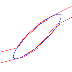
Figure 1: Cover an Ellipse with Slabs of Different Widths

The high-level idea is to build a two-level data structure. For the bottom-level, we build a multilevel simplex range reporting data structure [16] with query time $\tilde{O}(1)+O(k)$ and space $S(n)=\tilde{O}(n^{2})$. For the upper-level, for each cell $C$ in $G$ and a parameter $\alpha=2^{i}/Q(n)$, for $i=0,\cdots,\lfloor\log Q(n)\rfloor$, we generate a series of parallel disjoint slabs of width $\alpha/Q(n)$ such that they together cover $C$. Then we rotate these slabs by angle $\gamma=j/Q(n)$, for $j=1,2,\cdots,\lfloor 2\pi Q(n)\rfloor$. For each slab we generated during this process, we collect all the points in it and build a $\tilde{O}(Q(n)\alpha)+O(k)$ query time and $\tilde{O}((n/(Q(n)\alpha))^{\boldsymbol{m}})$ space data structure by linearization [19] to $\mathbb{R}^{\boldsymbol{m}}$ and using simplex range reporting [16].

The following lemma shows we can efficiently report the points close to $\partial\mathscr{R}$ using slabs we constructed. For the proof of this lemma, we refer the readers to Appendix F. lemmacellslabcover We can cut $\partial\mathscr{R}$ into a set $\mathcal{S}$ of $O(Q(n))$ sub-curves such that for each sub-curve $\sigma$, we can find a set $S_{\sigma}$ of slabs that together cover $\sigma$. Let $P_{\sigma}$ be the subset of the input that lies inside the query and inside the slabs, i.e., $P_{\sigma}=\mathscr{R}\cap\mathcal{P}\cap(\cup_{s\in S_{\sigma}}s)$. $P_{\sigma}$ can be reported in time $Q(n)\tilde{O}(\kappa_{\sigma}+1/Q(n))+O(|P_{\sigma}|)$, where $\kappa_{\sigma}$ is the total absolute curvature of $\sigma$. Furthermore, for any two distinct $\sigma_{1},\sigma_{2}\in\mathcal{S}$, $s_{1}\cap s_{2}=\emptyset$ for all $s_{1}\in S_{\sigma_{1}},s_{2}\in S_{\sigma_{2}}$.

With Lemma 1, we can bound the total query time for points close to $\partial\mathscr{R}$ by $\sum_{\sigma}Q(n)\tilde{O}(\kappa_{\sigma}+1/Q(n))+O(t_{\sigma})=\tilde{O}(Q(n))+O(t_{1}),$ where $t_{1}$ is the output size. An important observation is that after covering $\partial\mathscr{R}$, we can express the remaining regions by the boundaries of the slabs used and $G$, which are linear inequalities and so we can use simplex range reporting. Lemma 1 characterizes the remaining regions. See Appendix G for the proof. lemmalinregion There are $O(Q(n))$ remaining regions and each region can be expressed using $O(1)$ linear inequalities. These regions can be found in time $O(Q(n))$. With Lemma 1, the query time for the remaining regions is $\tilde{O}(Q(n))+O(t_{2})$, where $t_{2}$ is the number of points in the remaining regions. Then the total query time is easily computed to be bounded by $\tilde{O}(Q(n))+O(k)$, where $k=t_{1}+t_{2}$.

To bound the space usage for the top-level data structure, note that we have $Q(n)^{2}$ cells, for each $\alpha$, we generate $\Theta(\frac{1/Q(n)}{\alpha/Q(n)})=\Theta(1/\alpha)$ slabs for each of the $\Theta(Q(n))$ angles. Since points are distributed uniformly at random, the expected number of points in a slab of width $\alpha/Q(n)$ in a cell $C$ is $O(n\cdot\frac{1}{Q(n)}\cdot\frac{\alpha}{Q(n)})$. So the space usage for the top-level data structure is

$$S(n)=\sum_{\alpha}Q(n)^{2}\cdot\Theta\left(\frac{1}{\alpha}\right)\cdot\Theta(Q(n))\cdot\tilde{O}\left(\frac{O\left(n\cdot\frac{1}{Q(n)}\cdot\frac{\alpha}{Q(n)}\right)}{Q(n)\alpha}\right)^{\boldsymbol{m}}=\tilde{O}\left(\frac{n^{\boldsymbol{m}}}{Q(n)^{3\boldsymbol{m}-4}}\right).$$

On the other hand, we know that the space usage for the bottom-level data structure is $\tilde{O}(n^{2})$. So the total space usage is bounded by $\tilde{O}(\frac{n^{\boldsymbol{m}}}{Q(n)^{3\boldsymbol{m}-4}})$ for $\boldsymbol{m}\geq 3$.

We therefore obtain the following theorem.

Theorem 4.1.

Let $\mathcal{R}$ be the set of semialgebraic ranges formed by degree-$\Delta$ bivariate polynomials. Suppose we have a polynomial factorization black box that can factorize polynomials into the product of irreducible polynomials in time $O(1)$, then for any $\log^{O(1)}n\leq Q(n)\leq n^{\epsilon}$ for some constant $\epsilon$, and a set $\mathcal{P}$ of $n$ points distributed uniformly randomly in $\boldsymbol{U}=[0,1]\times[0,1]$, we can build a data structure of space $\tilde{O}(n^{\boldsymbol{m}}/Q(n)^{3\boldsymbol{m}-4})$ such that for any $\mathscr{R}\in\mathcal{R}$, we can report $\mathscr{R}\cap\mathcal{P}$ in time $\tilde{O}(Q(n))+O(k)$ in expectation, where $\boldsymbol{m}\geq 3$ is the number of parameters needed to define a degree-$\Delta$ bivariate polynomial and $k$ is the output size.

4.2 A Derivative-based Approach

If we assume that the derivative of $\partial\mathscr{R}$ is $O(1)$, the previous curvature-based approach can be easily adapted to get a derivative-based data structure. See Appendix H for details. We can even do better by using slabs whose boundaries are the zero set of higher degree polynomials instead of linear polynomials. Using Taylor’s theorem, we show that we can cover the boundary of the query using “thin” slabs of lower degree polynomials, similar to the approach above. The full details are presented in Appendix I.

Theorem 4.2.

Let $\mathcal{R}$ be the set of semialgebraic ranges formed by degree-$\Delta$ bivariate polynomials with bounded derivatives up to the $\Delta$-th order. For any $\log^{O(1)}n\leq Q(n)\leq n^{\epsilon}$ for some constant $\epsilon$, and a set $\mathcal{P}$ of $n$ points distributed uniformly randomly in $\boldsymbol{U}=[0,1]\times[0,1]$, we can build a data structure which uses space $\tilde{O}(n^{\boldsymbol{m}}/Q(n)^{((2\boldsymbol{m}-\Delta)(\Delta+1)-2)/2})$ s.t. for any $\mathscr{R}\in\mathcal{R}$, we can report $\mathcal{P}\cap\mathscr{R}$ in time $\tilde{O}(Q(n))+O(k)$ in expectation, where $\boldsymbol{m}$ is the number of parameters needed to define a degree-$\Delta$ bivariate polynomial and $k$ is the output size.

Remark 4.3.

We remark that our data structure can also be adapted to support semialgebraic range searching queries in the semigroup model.

5 Conclusion and Open Problems

In this paper, we essentially closed the gap between the lower and upper bounds of general semialgebraic range reporting in the fast-query case at least as far as the exponent of $n$ is concerned. We show that for general polynomial slab queries defined by $D$-variate polynomials of degree at most $\Delta$ in $\mathbb{R}^{D}$ any data structure with query time $n^{o(1)}+O(k)$ must use at least $S(n)=\overset{\scriptscriptstyle o}{\Omega}(n^{\boldsymbol{m}})$ space, where $\boldsymbol{m}=\binom{D+\Delta}{D}-1$ is the maximum possible parameters needed to define a query. This matches current upper bound (up to an $n^{o(1)}$ factor).

We also studied the space-time tradeoff and showed an upper bound that matches the lower bounds in [3] for uniform random point sets.

The remaining big open problem here is proving a tight bound for the exponent of $Q(n)$ in the space-time tradeoff. There is a large gap between the exponents in our lower bound versus the general upper bound. Our results show that current upper bound might not be tight. On the other hand, our lower bound seems to be suboptimal when the query time is $n^{\Omega(1)}+O(k)$. Both problems seem quite challenging, and probably require new tools.

Appendix A Proof of Theorem 2.1

*

First we present the original lower bound framework by Chazelle [11] and Chazelle and Rosenberg [13].

Theorem A.1.

Suppose the $D$-dimensional geometric range reporting problems admit an $S(n)$ space $Q(n)+O(k)$ query time data structure, where $n$ is the input size and $k$ is the output size. Assume we can find $m$ subsets $q_{1},q_{2},\cdots,q_{m}\subset\mathcal{S}$ for some input point set $\mathcal{S}$, where each $q_{i},i=1,\cdots,m$ is the output of some query and they satisfy the following two conditions: (i) for all $i=1,\cdots,m$, $|q_{i}|\geq Q(n)$; and (ii) $|q_{i_{1}}\cap q_{i_{2}}\cap\cdots q_{i_{\alpha}}|\leq c$ for some value $c\geq 2$. Then, we have $S(n)=\Omega(\frac{\sum_{i+1}^{m}|q_{i}|}{\alpha 2^{O(c)}})=\Omega(\frac{mQ(n)}{\alpha 2^{O(c)}})$.

A common way to use this framework is through a “volume” argument, i.e., we generate a set of geometric ranges in a hypercube and then show that they satisfy the following two properties:

• Each range intersects the hypercube with large Lebesgue measure;

• The Lebesgue measure of the intersection of any $k$ ranges is small.

Then if we sample $n$ points uniformly at random in the hypercube, we obtain $\mathcal{S}$ in thm:chazellefw in expectation. However, we generally want to show a lower bound for the worst case, then we need a way to derandomize to turn the result to a worst-case lower bound. We now introduce some derandomization techniques, which are direct generalizations of the $2$D version of the derandomization lemmas in [3]. Given a $D$-dimensional hypercube $\boldsymbol{C}^{D}$ of side length $|l|$ and a set of ranges. The first lemma shows that when each range intersects $\boldsymbol{C}^{D}$ with large $D$-dimensional Lebesgue measure (For simplicity, we will call such a measure $D$-measure and denoted by $\mu^{D}(\cdot)$.) and the number of ranges is not too big, then with high probability, each range will contain many points.

Lemma A.2.

Let $\boldsymbol{C}^{D}$ be a hypercube of side length $|l|$ in $\mathbb{R}^{D}$. Let $\mathcal{R}$ be a set of ranges in $\boldsymbol{C}^{D}$ satisfying two following conditions: (i) the $D$-measure of the intersection of any range $\mathscr{R}\in\mathcal{R}$ and $\boldsymbol{C}^{D}$ is at least $c|l|^{D}t/n$ for some constant $c\geq 4k$ and a parameter $t\geq\log n$ for some value $k\geq 2$; (ii) the total number of ranges is bounded by $O(n^{k+1})$. Now if we sample a set $\mathcal{P}$ of $n$ points uniformly at random in $\boldsymbol{C}^{D}$, then with probability $>1/2$, $|\mathcal{P}\cap\mathscr{R}|\geq t$ for all $\mathscr{R}\in\mathcal{R}$.

Proof A.3.

We pick $n$ points in $\boldsymbol{C}^{D}$ uniformly at random. Let $X_{ij}$ be the indicator random variable with

$$X_{ij}=\begin{cases}1,\textrm{point $i$ is in range $j$},\\ 0,\textrm{otherwise.}\end{cases}$$

Since $\mu^{D}(\mathscr{R})\geq c|l|^{D}t/n$ for every $\mathscr{R}\in\mathcal{R}$, the expected number of points in each range is at least $ct$. Consider an arbitrary range, let $X_{j}=\sum_{i=1}^{n}X_{ij}$, then by Chernoff’s bound

$$\Pr \left[X_{j}<\left(1-\frac{c-1}{c}\right)ct\right]<e^{-\frac{\left(\frac{c-1}{c}\right)^{2}ct}{2}}$$

$$\implies\Pr [X_{j}<t]<e^{-\frac{(c-1)^{2}t}{2c}}<\frac{1}{n^{\frac{(c-1)^{2}}{2c}}}\leq\frac{1}{n^{2k-1+1/(8k)}},$$

where the second last inequality follows from $t\geq\log n$ and the last inequality follows from $c\geq 4k$. Since the total number of ranges $O(n^{k+1})$, by the union bound, for $k\geq 2$ and a sufficiently large $n$, with probability $>\frac{1}{2}$, $|\mathcal{P}\cap\mathscr{R}|\geq t$ for all $\mathscr{R}\in\mathcal{R}$.

The second lemma tells a different story: when the $D$-measure of the intersection of any $k$ ranges is small, and the number of intersection is not too big, then with high probability, each intersection has very few points.

Lemma A.4.

Let $\boldsymbol{C}^{D}$ be a hypercube of side length $|l|$ in $\mathbb{R}^{D}$. Let $\mathcal{R}$ be a set of ranges in $\boldsymbol{C}^{D}$ satisfying the following two conditions: (i) the $D$-measure of the intersection of any $t\geq 2$ distinct ranges $\mathscr{R}_{1},\mathscr{R}_{2},\cdots,\mathscr{R}_{t}\in\mathcal{R}$ is bounded by $O(|l|^{D}/(n2^{\sqrt{\log n}}))$; (ii) the total number of intersections is bounded by $O(n^{2k})$ for $k\geq 1$. Now if we sample a set $\mathcal{P}$ of $n$ points uniformly at random in $\boldsymbol{C}^{D}$, then with probability $>1/2$, $|\mathscr{R}_{1}\cap\mathscr{R}_{2}\cap\cdots\cap\mathscr{R}_{t}\cap\mathcal{P}|<3k\sqrt{\log n}$ for all distinct ranges $\mathscr{R}_{1},\mathscr{R}_{2},\cdots,\mathscr{R}_{t}\in\mathcal{R}$.

Proof A.5.

We consider the intersection $\rho\in\boldsymbol{C}^{D}$ of any $t$ ranges and let $A=\mu^{D}(\rho)$. Let $X$ be an indicator random variable with

$$X_{i}=\begin{cases}1,\textrm{the $i$-th point is inside $\rho$},\\ 0,\textrm{otherwise.}\end{cases}$$

Let $X=\sum_{i=1}^{n}X_{i}$. Clearly, $\mathbb{E}[X]=\frac{An}{|l|^{D}}$. By Chernoff’s bound,

$$\Pr\left[X\geq(1+\delta)\frac{An}{|l|^{D}}\right]<\left(\frac{e^{\delta}}{(1+\delta)^{1+\delta}}\right)^{\frac{An}{|l|^{D}}},$$

for any $\delta>0$. Let $\tau=(1+\delta)\frac{An}{|l|^{D}}$, then

$$\Pr[X\geq\tau]<\frac{e^{\delta\frac{An}{|l|^{D}}}}{(1+\delta)^{\tau}}<\frac{e^{\tau}}{(1+\delta)^{\tau}}=\left(\frac{eAn}{|l|^{D}\tau}\right)^{\tau}.$$

Let $\tau=3k\sqrt{\log n}$, since $A\leq c|l|^{D}/(n2^{\sqrt{\log n}})$ for some constant $c$, we have

$$\Pr\left[X\geq 3k\sqrt{\log n}\right]<\left(\frac{ce}{2^{\sqrt{\log n}}3k\sqrt{\log n}}\right)^{3k\sqrt{\log n}}<\frac{(ce)^{3k\sqrt{\log n}}}{n^{3k}}.$$

Since the total number of intersections is bounded by $O(n^{2k})$, the number of cells in the arrangement is also bounded by $O(n^{2k})$ and thus by the union bound, for sufficiently large $n$, with probability $>\frac{1}{2}$, the number of points in every intersection region is less than $3k\sqrt{\log n}$.

We now prove Theorem 2.1.

Proof A.6.

We sample a set $\mathcal{P}$ of $n$ points uniformly at random in $\boldsymbol{C}^{D}$. Since each range $\mathscr{R}_{i}$ has $\mu^{D}(\mathscr{R}_{i})\geq 4c|l|^{D}Q(n)/n$, and the number of ranges is $m=n^{c}$, then by Lemma A.2, with probability more than $1/2$, $|\mathcal{P}\cap\mathscr{R}_{i}|\geq Q(n)$ for all $i=1,2,\cdots,m$. Since the intersection of any two ranges is upper bounded by $O(|l|^{D}/(n2^{\sqrt{\log n}}))$ and the total number of intersections is $O(m^{2})=O(n^{2c})$, then by Lemma A.4, with probability more than $1/2$, $|\mathscr{R}_{i}\cap\mathscr{R}_{j}\cap\mathcal{P}|=O(\sqrt{\log n})$ for distinct ranges $\mathscr{R}_{i},\mathscr{R}_{j}$. By the union bound, there is a point set such that both conditions in Theorem A.1 are satisfied, then we obtain a lower bound of

$$S(n)=\Omega\left(\frac{mQ(n)}{2\cdot 2^{O(\sqrt{\log n})}}\right)=\overset{\scriptscriptstyle o}{\Omega}(mQ(n)).$$

Appendix B Proof of Observation 3.3

*

Proof B.1.

We only need to show that there exists only one solution to equation $0=a_{1}-a_{2}^{\Delta}+f(a_{1})$ when $a_{1}>0$ and the solution has value $O(1)$, where $f(a_{1})$ is a polynomial in $a_{1}$ with nonnegative coefficients. Since $1\leq a_{2}\leq 2$, it easily follows.

Appendix C Proof of Lemma 3.3

*

Proof C.1.

Pick any point $p=(p_{1},p_{2},\cdots,p_{D})\in Z(P_{1})$, and $p^{\prime}=(p_{1}^{\prime},p_{2},\cdots,p_{D})\in Z(P_{2})$ such that $p_{i}\in[1,2]$ for all $i=2,3,\cdots,D$, and $p_{1}^{\prime}=p_{1}+\gamma$. Clearly, $0<\gamma<1$ because $0\leq r=O(w)=o(1)$. By definition

$$P_{2}(p^{\prime})=p_{1}+\gamma+p_{2}^{D}+\left(\sum_{i}A_{i}(p_{1}+\gamma)^{i_{1}}p_{2}^{i_{2}}p_{3}^{i_{3}}\cdots p_{D}^{i_{D}}\right)-r=P_{1}(p)+\Theta(\gamma)-r=0.$$

So $\gamma=\Theta(r)$, meaning, $\pi(Z(P_{1}),Z(P_{2}),p)=\Theta(r)$ for $X\in[1,2]^{D-1}$.

Appendix D Proof of Lemma 3.3

*

We first bound the length of the $y$-interval within which a packed bivariate can intersect $\boldsymbol{U}^{2}$.

Lemma D.1.

Let $P$ be a packed bivariate polynomial. Then $\sigma=Z(P)$ is fully contained in $\boldsymbol{U}^{2}$ for some $y$-interval of length $\Theta(1)$.

Proof D.2.

We show that $\sigma$ is sandwiched by curves $\sigma_{l}:x-y^{\Delta}+c\epsilon=0$ for some sufficiently large constant $c$ and $\sigma_{r}:x-y^{\Delta}=0$ in $\boldsymbol{U}^{2}$. We intersect $\sigma_{l},\sigma,\sigma_{r}$ with line $y=y_{*}$ for $y_{*}\in[1,2]$ and denote the intersections to be $(x_{l},y_{*}),(x_{m},y_{*}),(x_{r},y_{*})$ respectively. Since $\sigma$ is of form $x-y^{\Delta}+\sum_{i=0}^{\Delta}\sum_{j=0}^{\Delta-i}c_{ij}x^{i}y^{j}=0$, $x_{m}=y_{*}^{\Delta}-O(\epsilon)$ because $0\leq c_{ij}=O(\epsilon)$ and $0<x=O(1)$ when $y_{*}\in[1,2]$ by Observation 3.3. So for sufficiently large $c$, $x_{l}\leq x_{m}\leq x_{r}$. It is elementary to compute that $\sigma_{l}$ and $\sigma_{r}$ intersect $x=1$ at point $(1,\sqrt[\Delta]{1+c\epsilon}),(1,1)$ respectively, and intersect $x=2$ at point $(2,\sqrt[\Delta]{2+c\epsilon}),(2,\sqrt[\Delta]{2})$ respectively in the first quadrant. So the intersection of $\sigma$ with $x=1$ (resp. $x=2$) has $y$-value between $1$ and $\sqrt[\Delta]{1+c\epsilon}$ (resp. $\sqrt[\Delta]{2}$ and $\sqrt[\Delta]{2+c\epsilon}$). So the projection of $\sigma\cap\boldsymbol{U}^{2}$ onto the $y$-axis has length at least $\sqrt[\Delta]{2}-\sqrt[\Delta]{1+c\epsilon}$. Since $\epsilon=o(1)$, the lemma holds.

Now we prove Lemma 3.3.

Proof D.3.

We intersect $Z(P)$ with $X_{i}=a_{i}\in[1,2]$ for $i=3,4,\cdots,D$. The resulting polynomial will be a packed bivariate polynomial. By Lemma D.1, we know the intersection of the zero set of this bivariate polynomial and $\boldsymbol{U}^{2}$ has $1$-measure $\Theta(1)$ in the $X_{2}$-axis. Integrating over all $X_{i}$ for $i=3,4,\cdots,5$, $Z(P)$ intersects $\boldsymbol{U}^{D}$ with $(D-1)$-measure $\Theta(1)$ in the subspace perpendicular to the $X_{1}$-axis.

Appendix E Total Absolute Curvature of the Zero Set of Irreducible Polynomials

In this section, we prove the following lemma.

Lemma E.1.

Let $P$ be an irreducible bivariate polynomial of constant degree. Then $Z(P)$ has total absolute curvature $O(1)$.

We first show for any value $v\in\mathbb{R}\cup\{\pm\infty\}$, the number of points on $Z(P)$ whose derivative achieves this value is $O(1)$.

We will use Bézout’s Thoerem.

Theorem E.2 (Bézout’s Theorem).

Given $2$ polynomials $P(x,y)$ and $Q(x,y)$ of degree $\Delta_{p}$ and $\Delta_{q}$ respectively, either the number of common zeroes of $P$ and $Q$ is at most $\Delta_{p}\cdot\Delta_{q}$ or they have a common factor.

Now we show any irreducible polynomial has $O(1)$ points achieving the same derivative.

Lemma E.3.

Let $P(x,y)$ be an irreducible bivariate polynomial of degree $\Delta>1$. Then the number of points on $Z(P(x,y))$ which have a fixed derivative $c$ is bounded by $O(\Delta^{2})$.

Proof E.4.

For simplicity, we first rotate $P(x,y)$ such that the fixed derivative is $0$. Let us denote the new polynomial with $Q(x,y)$ and it is easy to see that $Q$ is also irreducible since if $Q$ could be written as $Q(x,y)=R(x,y)S(x,y)$, then $P(x,y)$ would also have a similar decomposition.

By differentiating $Q$, we get that $\frac{\differential y}{\differential x}=-\frac{Q_{x}(x,y)}{Q_{y}(x,y)}=0$, and thus $Q_{x}(x,y)=0$. As a result, any point $(x,y)$ with derivative 0, lies on the zero set of $Q$ and $Q_{x}$.

Both $Q$ and $Q_{x}$ have degree $O(\Delta)$ and since $Q$ is irreducible and degree of $Q_{x}$ is at least one, they cannot have a common factor. By Bézout’s Theorem, this implies that they have $O(\Delta^{2})$ common zeroes.

We now prove Lemma E.1. More specifically, we prove the following:

Lemma E.5.

Consier a smooth curve $C$ such that for any value $v$, there are at most $k$ points $p$ on $C$ such that the tangent line at $p$ has slope $v$. Then $C$ has total absolute curvature $O(k^{2})$.

Proof E.6.

We parametrize $P(x,y)=0$ by its arc length $s$ over an interval $I$ and then consider the function $\alpha:\mathbb{R}\rightarrow\mathbb{R}$ be a function that maps the arc length of the curve to the angle of the curve. Note that $\alpha(s)$ is allowed to increase beyond $2\pi$. Let $\alpha_{1}$ and $\alpha_{2}$ be the infimum and surpremum of $\alpha(s)$ over $s\in I$. Note that we must have $\alpha_{2}-\alpha_{1}\leq k2\pi$ as otherwise we can find more then $k$ points with the same slope on $C$. $\alpha^{\prime}(s)$ determines the curvature of the curve at point $s$ and its total curvature is

$$\int_{I}|\alpha^{\prime}(s)|ds\leq 2\pi k^{2}$$

where the inequality follows from the observation that the equation $\alpha(s)=v$ for every $v$ has at most $k$ solutions and thus the total change in $\alpha(s)$ is bounded by $k\cdot|\alpha_{2}-\alpha_{1}|\leq 2\pi k^{2}$.

Lemma E.1 then follows easily by Lemma E.3 and E.5.

Appendix F Proof of Lemma 1

*

Now suppose we have a sub-curve $\sigma\subset\partial\mathscr{R}$ in $C$ that contains no singular points (points with undefined derivatives) except for possible the two boundaries, if the total absolute curvature is between $0$ and $\pi/4$, then we can efficiently find $O(1)$ slabs to cover it as shown in the following lemma.

Lemma F.1.

Let $\sigma$ be any differentiable sub-curve in a cell $C$ with total absolute curvature $\kappa_{\sigma}$ such that $0\leq\kappa_{\sigma}\leq\pi/4$. We can find a set of $O(1)$ slabs of width $O(\kappa_{\sigma}/Q(n)+1/Q(n)^{2})$ that together cover $\sigma$ and these slabs can be found in time $\tilde{O}(1)$.

Proof F.2.

Let $p$ and $q$ be the end points of the curve $\sigma$. Consider the point $r$ furthest away from the line $pq$ on the curve. See Figure 2 for an example. Observe that we can use the mean value theorem between $p$ and $r$ and also between $r$ and $q$. This yields that the sum of the angles $\angle rpq+\angle rqp$ is at most the total absolute curvature of $\sigma$. Since $p,q$ are in $C$, $|\overline{pq}|=O(1/Q(n))$ and since $\angle rpq,\angle rqp\leq\kappa_{\sigma}\leq\pi/4$, it follows that the distance between the line tangent to $r$ and $\overline{pq}$ is $O(\kappa_{\sigma}/Q(n))$. Finally, notice that in our construction, we have created slabs of orientation $i/Q(n)$ for every integer $i$. As a result, we can cover $\sigma$ with $O(1)$ slabs of width $O(\kappa_{\sigma}/Q(n)+1/Q(n)^{2})$. To find the slabs, we can use any of the previous techniques in semialgebraic range searching since the input size (i.e., the number of slabs) in our construction is $Q(n)^{O(1)}$.

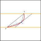
Figure 2: Covering a Sub-curve Using Slabs

We now show how to decompose $\partial\mathscr{R}$. Observe that $\partial\mathscr{R}$ intersects $O(Q(n))$ cells in $G$ because otherwise $\partial\mathscr{R}$ will have $\omega(1)$ tangents, which contradicts Bézout’s theorem. We cut $\partial\mathscr{R}$ using these $O(Q(n))$ cells to get $\mathcal{S}$.

Let $\sigma\subset\partial\mathscr{R}$ be the sub-curve in a cell $C\in G$. To find slabs to cover $\sigma$, we refine $\sigma$ to be smaller pieces of curves to use Lemma F.1. We simply cut $\sigma$ into pieces such that each piece has total absolute curvature $\leq\pi/4$ and contains no singular points. Recall that the singular points of the zero set of a bivariate polynomial is a point where both partial derivatives are $0$. By Bézout’s theorem, there are $O(1)$ singular points. Since the total curvature of $\partial\mathscr{R}$ is $O(1)$, we will get $O(1)$ refined sub-curves. This part is easy with the assumption of our model of computation and so we omit the details about how to cut $\sigma$.

Now for each (refined) sub-curve $\sigma_{r}$, by Lemma F.1 we can find $O(1)$ slabs to cover it. We report points close to $\sigma_{r}$ as follows. First we sort the slabs in some order. Let $s$ be a slab we find for $\sigma_{r}$. When we examine $s$, we use the data structure built in $s$ to find the points in $\mathscr{R}$. The query time will be $Q(n)\tilde{O}(\kappa_{\sigma_{r}}+1/Q(n))+O(k)$ by Lemma F.1. Before reporting the point, we check if the point has been reported in slabs we have examined before. This is because the slabs we found may intersect. But since we have $O(1)$ refined sub-curves for $\sigma$ and each refined sub-curve requires $O(1)$ slabs to cover, it takes only $O(1)$ time to check for duplicates. Summing up the query cost for all refined sub-curves for $\sigma$, the total query time is $Q(n)\tilde{O}(\kappa_{\sigma}+1/Q(n))+O(t_{\sigma})$. Since cells in $G$ are disjoint and each slab is built only for a specific cell, the slabs we find for two distinct sub-curves will have zero intersection. This proves Lemma 1.

Appendix G Proof of Lemma 1

*

There are two types of remaining regions. First, cells fully contained in $\mathscr{R}$ but do not intersect $\partial\mathscr{R}$. Second, the regions in a cell intersected by $\partial\mathscr{R}$ but not covered by slabs.

We first handle the first type. For any two adjacent vertical lines $l_{1},l_{2}$ in the grid $G$, we find all the cells between them intersected by $\partial\mathscr{R}$ in decreasing order with respect to their $y$-coordinates. For two consecutive cells $C_{1},C_{2}$ we find, all the cells between $C_{1},C_{2}$ must be all contained or all not contained in $\mathscr{R}$ because otherwise $C_{1},C_{2}$ are not adjacent. We then express the union of cells in between $C_{1},C_{2}$ using four linear inequalities. By this, we can find all the cells intersecting $\partial\mathscr{R}$ and all the chunks of cells fully contained in $\mathscr{R}$ between $l_{1},l_{2}$. We do this for every consecutive pair of vertical lines. The number of chunks is linear to the number of cells intersecting $\partial\mathscr{R}$ which is $O(Q(n))$ by Bézout’s theorem, so we have $O(Q(n))$ chunks as well. See Figure 3 (a) for an example.

For the second type, observe that each such region is defined by the boundaries of $C$ (and/or) the outermost boundaries of slabs we used to cover sub-curves. Since by the analysis of Lemma 1, the sub-curve in a cell $C$ requires only $O(1)$ slabs to cover. The outmost boundaries of these $O(1)$ slabs form a subdivision of complexity $O(1)$. Since each face in the subdivision is either fully contained in $\mathscr{R}$ or not contained in $\mathscr{R}$, it suffices to check an arbitrary point in the face. We omit the details here. In one cell, we have $O(1)$ remaining regions (faces in the subdivision) and it takes $O(1)$ time to find it. Since $\partial\mathscr{R}$ intersects $O(Q(n))$ regions, there are $O(Q(n))$ regions in total and it takes $O(Q(n))$ time to find them. See Figure 3 (b) for an example. This proves Lemma 1.

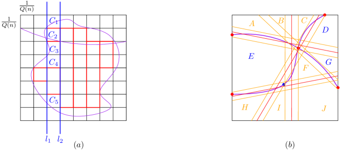
Figure 3: To Answer a Query: $(a)$: Finding cells fully contained in $\partial\mathscr{R}$. We have a chunk of zero cell between pairs $(C_{1},C_{2})$, $(C_{2},C_{3})$, and $(C_{3},C_{4})$, and a chunk of two cells between $C_{4},C_{5}$. $(b)$: Covering a sub-curve $\sigma$ in a cell. Red dots are singular points of $\partial\mathscr{R}$ and its intersections with $C$. The blue dots is used to make sure each refined sub-curve has total absolute curvature $\leq\pi/4$. We use slabs (denoted by orange/red line segments) to cover the boundaries of $\sigma$. There are $10$ regions in the subdivision formed by the outmost boundaries of slabs. Three of them $(D,E,G)$ are fully contained in $\mathscr{R}$.

Appendix H An $S(n)=\tilde{O}(n^{\boldsymbol{m}}-Q(n)^{3\boldsymbol{m}-4})$ Derivative-based Data Structure

The data structure is similar to the curvature-based one. We also build a two-level data structure. For each cell $C$, we “guess” $Q(n)$ first derivatives $\alpha_{1}=-c,-c+t,-c+2t,\cdots,c$, for $t=2c/Q(n)$. For each guess $\alpha_{1}$, we generate a series of disjoint parallel slabs of (vertical) width $w_{v}=1/Q(n)^{2}$ each that together cover $C$ such that the boundary of each slab has derivative $\alpha_{1}$. Since $|\alpha_{1}|=O(1)$, the angle $\gamma$ between any slab and the $x$-axis is also $O(1)$, so the width of each slab is $w=w_{v}\cdot\cos\gamma=\Theta(w_{v})$. Therefore the total number of slabs we generate for each $\alpha_{1}$ in a cell is $\frac{\Theta(1/Q(n))}{\Theta(w_{v})}=O(Q(n))$. For each $s$, we collect the points in it and build an $\tilde{O}(1)+O(k)$ query time and $\tilde{O}(n^{\boldsymbol{m}})$ space data structure. This is our top-level data structure. For the bottom-level data structure, we still use a multilevel simplex range reporting data structure with $\tilde{O}(n^{2})$ space and $\tilde{O}(1)+O(k)$ query time.

The space usage for the top level data structure is easily bounded to be

$$S_{1}(n)=\tilde{O}\left(Q(n)^{2}\cdot\frac{2c}{2c/Q(n)}\cdot O(Q(n))\cdot\left(\frac{1}{Q(n)^{2}}\cdot\frac{1}{Q(n)}\cdot n\right)^{\boldsymbol{m}}\right)=\tilde{O}\left(\frac{n^{\boldsymbol{m}}}{Q(n)^{3\boldsymbol{m}-4}}\right).$$

Since the bottom level data structure takes up $\tilde{O}(n^{2})$ space. The total space usage is $\tilde{O}(\frac{n^{\boldsymbol{m}}}{Q(n)^{3\boldsymbol{m}-4}})$ for $\boldsymbol{m}\geq 3$.

For the query answering, we prove a lemma similar to Lemma F.1.

Lemma H.1.

In our construction, if some differentiable sub-curve $\sigma$ is contained in $C$, then we can find $O(1)$ slabs that cover $\sigma$. The time needed to find all these slabs is $\tilde{O}(1)$.

Proof H.2.

Let $(p_{x},p_{x}),(q_{x},q_{y})$ be the left and right endpoints of $\sigma$ and $\frac{\differential y}{\differential x}(p_{x},p_{y})=\alpha_{1}^{*}$. Let $f(x)$ be the implicit function defined by $\sigma$ in between $(p_{x},p_{y})$ and $(q_{x},q_{y})$. Let $g(x)=\alpha_{1}(x-p_{x})+p_{y}$ be the line passing through $(p_{x},p_{y})$ with slope $\alpha_{1}$. Define the vertical distance between $f(x)$ and $g(x)$ in $[p_{x},q_{x}]$ to be $d(x)=f(x)-g(x).$ Since we guess $\alpha_{1}=\frac{\differential y}{\differential x}(p_{x},p_{y})$ with step size $2\pi/Q(n)$,

$$d(x) =f(x)-(\alpha_{1}(x-p_{x})+p_{y})$$

$$\leq f(x)-((\alpha_{1}^{*}\pm 2c/Q(n))(x-p_{x})+p_{y})$$

$$=(f(x)-\alpha_{1}^{*}(x-p_{x})-p_{y})\pm 2c/Q(n)(x-p_{x})$$

$$=\frac{f^{(2)}(\xi)}{2!}(x-p_{x})^{2}\pm 2c/Q(n)(x-p_{x}),$$

for some constant $\xi$ between $p_{x}$ and $x$, where the last equality follows from Taylor’s theorem. Since $x\in[p_{x},q_{x}]$ and $|q_{x}-p_{x}|\leq 1/Q(n)$ as they are in $C$ and all the derivatives are bounded, $|d(x)|=O(1/Q(n)^{2})$. Since each slab has vertical width $w_{v}=1/Q(n)^{2}$, we only need $O(1)$ slabs to cover $\sigma$.

To find these slabs, by a similar analysis as in Lemma F.1, since there are only $Q(n)^{O(1)}$ slabs in total, we can build a simple $Q(n)^{O(1)}$ size searching data structure to find the $O(1)$ slabs in time $\tilde{O}(1)$.

Having Lemma H.1 in hand, the query process is essentially the same as the one for the curvature-based solution and the analysis is also the same by replacing Lemma F.1 by Lemma H.1. We omit the deials and present the following theorem.

Theorem H.3.

Let $\mathcal{R}$ be the set of semialgebraic ranges formed by degree-$\Delta$ bivariate polynomials with bounded derivatives up to the $\Delta$-th order. For any $\log^{O(1)}n\leq Q(n)\leq n^{\epsilon}$ for some constant $\epsilon$, and a set $\mathcal{P}$ of $n$ points distributed uniformly randomly in $\boldsymbol{U}=[0,1]\times[0,1]$, we can build a data structure of space $\tilde{O}(n^{\boldsymbol{m}}/Q(n)^{3\boldsymbol{m}-4})$ such that for any $\mathscr{R}\in\mathcal{R}$, we can report $\mathscr{R}\cap\mathcal{P}$ in time $\tilde{O}(Q(n))+O(k)$ in expectation, where $\boldsymbol{m}$ is the number of parameters needed to define a degree-$\Delta$ bivariate polynomial and $k$ is the output size.

Remark H.4.

Note that we actually only need bounded derivatives up to the second order in Theorem H.3.

Appendix I An $S(n)=\tilde{O}(n^{\boldsymbol{m}}/Q(n)^{((2\boldsymbol{m}-\Delta)(\Delta+1)-2)/2})$ Derivative-based Data Structure

Now we improve the results in Appendix H. The main idea is to use slabs formed by higher degree polynomial equalities. These slabs work as finer and finer approximations to the boundaries of query ranges. We first define some notations.

Definition I.1.

Let $I_{x}=[x_{l},x_{r}]$ be an interval in the $x$-axis. Let $U(x)$ and $L(x)$ be two degree-$i$ polynomials in $x$ such that $\forall x\in I_{x},U(x)>L(x)$. We say that the region enclosed by $U(x)$, $L(x)$, $x=x_{l}$ and $x=x_{r}$ is an $i$-slab $s$. We also say the $x$-range of $s$ is $[x_{l},x_{r}]$. Furthermore, if for all $x\in I_{x}$, $U(x)-L(x)=w$, we say $s$ is a uniform slab with width $w$.

In our application, $L(x),U(x)$ will be two degree-$i$ polynomial functions that differ only in their constant terms. It is not hard to see that in this case, all the slabs are in fact uniform.

In a nutshell, our data structure $\Psi_{\Delta}$ for degree-$\Delta$ polynomial inequalities is still a two-level data structure. The top-level structure is similar to that we described in Appendix H but instead of using $1$-slabs, we use $(\Delta-1)$-slabs. These $(\Delta-1)$-slabs will have width $1/Q(n)^{\Delta}$ and we build data structures of size $\tilde{O}(n^{\boldsymbol{m}_{2,\Delta}})$ for the points in each slab that can answer semialgebraic queries defined by degree-$\Delta$ polynomial inequalities in $\tilde{O}(1)+O(k)$ time. The second part is a data structure built for the entire input points and it can answer degree-$(\Delta-1)$ polynomial inequality queries in time $\tilde{O}(1)+O(k)$ with space usage $\tilde{O}(n^{\boldsymbol{m}_{2,\Delta-1}})$. The overall idea of our data structure is the following: given $\mathscr{R}$, we use $(\Delta-1)$-slabs to cover its boundary. Then the remaining parts will be defined by degree-$(\Delta-1)$ polynomial inequalities. So we can use the bottom-level data structure to solve them.

Now we describe the details. We first describe how to generate $i$-slabs for $i=1,2,\cdots,\Delta-1$. The base $1$-slabs are what we have described in Appendix H. Now assume we already have an $(i-1)$-slab $s_{i-1}$, we generate $i$-slabs as follows. Let the $x$-range of $s_{i-1}$ be $[x_{l},x_{r}]$. Let $\alpha_{j}^{l}=\frac{\differential^{j}y}{\differential x^{j}}(x_{l})$ for $j=1,2,\cdots,i-1$ be the $j$-th order derivatives of $L(x)$ of $s_{i-1}$ at $x=x_{l}$. Now to construct $L(x)$ of an $i$-slab $s_{i}$, we make $Q(n)$ finer guesses for each $\frac{\differential^{j}y}{\differential x^{j}}(x_{l})$. Specifically, $\frac{\differential^{j}y}{\differential x^{j}}(x_{l})=\alpha_{j}^{l},\alpha_{j}^{l}+\frac{2c}{Q(n)^{i-j+1}},\alpha_{j}^{l}+2\cdot\frac{2c}{Q(n)^{i-j+1}},\cdots,\alpha_{j}^{l}+\frac{2c}{Q(n)^{i-j}}$, for $j=1,2,\cdots,i-1$, and $\frac{\differential^{i}y}{\differential x^{i}}(x_{l})=-c+\frac{2c}{Q(n)},-c+2\cdot\frac{2c}{Q(n)},\cdots,c$. We then place “anchor” points evenly spaced with distance $1/Q(n)^{i+1}$ on the left boundary of $s_{i-1}$. Every two degree-$i$ polynomials passing through adjacent anchor points having the same $\frac{\differential^{j}y}{\differential x^{j}}(x_{l})$ for $j=1,2,\cdots,i$ defines an $i$ slab. If any two degree-$i$ polynomials $P(x),Q(x)$ have the same $k$-th derivatives for all $k=1,2,\cdots,i$ at two points $(x_{l},y_{1})$, $(x_{l},y_{2})$, it is elementary to show that for all $x$, $|P(x)-Q(x)|=|y_{1}-y_{2}|$. So every $i$-slab is uniform and its width is $1/Q(n)^{i+1}$.

To build $\Psi_{\Delta}$, we first build $1$-slabs as we did in Appendix H, and then repeatedly applying the process described in the previous paragraph to get degree-$(\Delta-1)$ slabs. Then we build the $\tilde{O}(n^{\boldsymbol{m}_{2,\Delta}})$ space data structure in each slab as the top-level data structure, and then build the $\tilde{O}(n^{\boldsymbol{m}_{2,\Delta-1}})$ space data structure for all input points as the bottom-level data structure.

Now we bound the space usage. By the above procedure, for each $(i-1)$-slab, $i\geq 3$ we generate $Q(n)^{i-2}$ guesses for derivatives for the first $i-2$ derivatives, and $Q(n)$ guesses for the $(i-1)$-th derivative. We have $\frac{1/Q(n)^{i-1}}{1/Q(n)^{i}}=Q(n)$ anchor points for the lower boundaries of slabs to pass through. So in total, we generate $Q(n)^{i-2}\cdot Q(n)\cdot Q(n)=Q(n)^{i}$ many $(i-1)$-slabs in an $(i-2)$-slab. We know from Appendix H that the number of $1$-slabs is upper bounded by $O(Q(n)^{4})$. Since we only build fast-query data structures in $(i-1)$-slabs, the total space usage of all the structures built on $(i-1)$-slabs is then bounded by

$$S_{1}(n) =O\left(Q(n)^{4}\cdot\left(\prod_{j=3}^{i}Q(n)^{j}\cdot\right)\cdot\left(\frac{1}{Q(n)^{i}}\cdot\frac{1}{Q(n)}\cdot n\right)^{\boldsymbol{m}_{2,i}}\right)$$

$$=O\left(Q(n)^{(i+1)i/2+1}\cdot\frac{n^{\boldsymbol{m}_{2,i}}}{Q(n)^{\boldsymbol{m}_{2,i}(i+1)}}\right)$$

$$=O\left(\frac{n^{\boldsymbol{m}_{2,i}}}{Q(n)^{((2\boldsymbol{m}_{2,i}-i)(i+1)-2)/2}}\right).$$

As mentioned before, the space usage of the bottom-level data structure for $\Psi_{i}$ is $\tilde{O}(n^{\boldsymbol{m}_{2,i-1}})$. Then for query time $Q(n)=n^{\epsilon}$ where $\epsilon$ is some small constant, the space usage of our entire data structure $\Psi_{i}$ is bounded by $\tilde{O}(n^{\boldsymbol{m}_{2,i}}/Q(n)^{((2\boldsymbol{m}_{2,i}-i)(i+1)-2)/2})$.

For query answering, we first show the following lemma, which is a generalization of Lemma H.1. The proof idea is similar to Lemma H.1, the only difference is now we consider a Taylor polynomial of degree-$(\Delta-1)$ instead of $1$.

Lemma I.2.

In our construction, if some differentiable sub-curve $\sigma$ is contained in some cell $C$, then we can find up to $O(1)$ $(\Delta-1)$-slabs to cover $\sigma$. The time needed to find these slabs is $\tilde{O}(1)$.

Proof I.3.

Let $(p_{x},p_{y}),(q_{x},q_{y})$ be the left and right endpoints of $\sigma$ and $\frac{\differential^{i}y}{\differential x^{i}}(p_{x},p_{y})=\alpha_{i}^{*}$ for $i=1,2,\cdots,\Delta-1$. Let $f(x)$ be the implicit function defined by $\sigma$ in $[p_{x},q_{x}]$ and let $g(x)$ be a degree-$\Delta$ polynomial whose first $\Delta$ derivatives agree with those of $f(x)$ at point $(p_{x},p_{y})$. By Taylor’s theorem, the vertical distance between $f(x)$ and $g(x)$ is easily calculated to be bounded by $O(1/Q(n)^{\Delta+1})$ in $[p_{x},q_{x}]$. Next we bound the vertical distance between $g(x)$ and the best fitting polynomial in our construction. Let $(a,b)$ be the intersection of $g(x)$ with the line containing the left boundary of $C$. Let $h(x)=\sum_{i=1}^{\Delta-1}\frac{\alpha_{i}}{i!}(x-a)^{i}+b$ be a degree-$(\Delta-1)$ polynomial passing through $(a,b)$ with $i$-th order derivative being $\alpha_{i}$ at $x=a$. We define the vertical distance between $g(x)$ and $h(x)$ in this range to be $d(x)=g(x)-h(x).$

Since we guess $\alpha_{i}=\frac{\differential^{i}y}{\differential x^{i}}$ at $x=a$ with step size $2c/Q(n)^{\Delta-i}$ in our construction,

$$d(x) =g(x)-\left(\sum_{i=1}^{\Delta-1}\frac{\alpha_{i}}{i!}(x-a)^{i}+b\right)$$

$$\leq g(x)-\left(\sum_{i=1}^{\Delta-1}\left(\frac{\alpha_{i}^{*}\pm 2c/Q(n)^{\Delta-i}}{i!}\right)(x-a)^{i}+b\right)$$

$$=\left(g(x)-\left(\sum_{i=1}^{\Delta-1}\frac{\alpha_{i}^{*}}{i!}(x-a)^{i}+b\right)\right)\pm\sum_{i=1}^{\Delta-1}\frac{2c/Q(n)^{\Delta-i}}{i!}(x-a)^{i}$$

$$=\frac{g^{(\Delta)}(\xi)}{\Delta!}(x-a)^{\Delta}\pm\sum_{i=1}^{\Delta-1}\frac{2c/Q(n)^{\Delta-i}}{i!}(x-a)^{i}$$

for some constant $\xi$ between $a$ and $x$, where the last equality follows from Taylor’s theorem. Since $x\in[a,q_{x}]$ and $|q_{x}-a|\leq 1/Q(n)$ and all the derivatives of $g(x)$ are bounded in $\boldsymbol{U}$, $|d(x)|=O(1/Q(n)^{\Delta})$. Then the distance between $f(x)$ and $h(x)$ is bounded by $O(1/Q(n)^{\Delta+1})+|d(x)|=O(1/Q(n)^{\Delta})$ in $[p_{x},q_{x}]$. Since each $(\Delta-1)$-slab has width $1/Q(n)^{\Delta}$, so it takes $O(1)$ $(\Delta-1)$-slabs to cover $\sigma$. To find these slabs, by a similar analysis as in Lemma F.1, since there are only $Q(n)^{O(1)}$ slabs in total, we can build a simple $Q(n)^{O(1)}$ size searching data structure to find the $O(1)$ slabs in time $\tilde{O}(1)$.

With Lemma I.2 in hand, the query algorithm is essentially the same as the data structure described in Appendix F except for one minor difference: here when we answer query in some cell, we find $(\Delta-1)$-slabs and use the fast query data structure in it. But now since the boundaries of slabs are degree-$(\Delta-1)$ polynomials, we need to handle ranges defined by $(\Delta-1)$ polynomial inequalities instead of linear inequalities. This can be handled by our bottom-level data structure. By a similar analysis as in Appendix F, we can find $O(Q(n))$ $(\Delta-1)$-slabs to cover $\partial\mathscr{R}$. We can then report all the points close to $\partial\mathscr{R}$ in time $\tilde{O}(Q(n))+O(k)$. The remaining regions of $\mathscr{R}$ are defined by $O(Q(n))$ boundaries of the slabs we used and $G$ by a similar analysis as in Appendix G. We use the bottom-level data structure for this part and again we need $\tilde{O}(Q(n))+O(k)$ time to report the points. In total, the query time is bounded by $\tilde{O}(Q(n))+O(k)$. This proves Theorem 4.2.

Specifically, for polynomial inequalities of form $y+\sum_{a_{i}}x^{i}\leq 0$ or $x+\sum_{a_{i}}y^{i}\leq 0$, where $a_{i}\in\mathbb{R}$ and $0\leq i\leq\Delta$ is an integer, we have:

Theorem I.4.

For Semialgebraic range $\mathscr{R}$ formed by polynomial inequalities of form $y+\sum_{a_{i}}x^{i}\leq 0$ or $x+\sum_{a_{i}}y^{i}\leq 0$, where $a_{i}\in\mathbb{R}$ and $0\leq i\leq\Delta$ is an integer, and any $\log^{O(1)}n\leq Q(n)\leq n^{\epsilon}$ for some constant $\epsilon$, if the $n$ input points are distributed uniformly randomly in a unit square $\boldsymbol{U}=[0,1]\times[0,1]$, we can build a data structure of space $\tilde{O}(n^{\Delta+1}/Q(n)^{(\Delta+3)\Delta/2})$ that answers range reporting queries with $\mathscr{R}$ in time $\tilde{O}(Q(n))+O(k)$ in expectation, where $k$ is the number of points to report.

References

- [1] Peyman Afshani. Improved pointer machine and I/O lower bounds for simplex range reporting and related problems. In Proceedings of the Twenty-Eighth Annual Symposium on Computational Geometry, SoCG ’12, page 339–346, New York, NY, USA, 2012. Association for Computing Machinery. \hrefhttps://doi.org/10.1145/2261250.2261301 \pathdoi:10.1145/2261250.2261301.
- [2] Peyman Afshani. A new lower bound for semigroup orthogonal range searching. In 35th International Symposium on Computational Geometry, volume 129 of LIPIcs. Leibniz Int. Proc. Inform., pages Art. No. 3, 14. Schloss Dagstuhl. Leibniz-Zent. Inform., Wadern, 2019.
- [3] Peyman Afshani and Pingan Cheng. Lower Bounds for Semialgebraic Range Searching and Stabbing Problems. In Kevin Buchin and Éric Colin de Verdière, editors, 37th International Symposium on Computational Geometry (SoCG 2021), volume 189 of Leibniz International Proceedings in Informatics (LIPIcs), pages 8:1–8:15, Dagstuhl, Germany, 2021. Schloss Dagstuhl – Leibniz-Zentrum für Informatik. URL: \urlhttps://drops.dagstuhl.de/opus/volltexte/2021/13807, \hrefhttps://doi.org/10.4230/LIPIcs.SoCG.2021.8 \pathdoi:10.4230/LIPIcs.SoCG.2021.8.
- [4] Pankaj K. Agarwal. Simplex range searching and its variants: a review. In A journey through discrete mathematics, pages 1–30. Springer, Cham, 2017.
- [5] Pankaj K. Agarwal, Boris Aronov, Esther Ezra, and Joshua Zahl. Efficient algorithm for generalized polynomial partitioning and its applications. SIAM J. Comput., 50(2):760–787, 2021. \hrefhttps://doi.org/10.1137/19M1268550 \pathdoi:10.1137/19M1268550.
- [6] Pankaj K. Agarwal, Jiří Matoušek, and Micha Sharir. On range searching with semialgebraic sets. II. SIAM J. Comput., 42(6):2039–2062, 2013. \hrefhttps://doi.org/10.1137/120890855 \pathdoi:10.1137/120890855.
- [7] Sunil Arya, Theocharis Malamatos, and David M. Mount. On the importance of idempotence. In STOC’06: Proceedings of the 38th Annual ACM Symposium on Theory of Computing, pages 564–573. ACM, New York, 2006. \hrefhttps://doi.org/10.1145/1132516.1132598 \pathdoi:10.1145/1132516.1132598.
- [8] Sunil Arya, David M. Mount, and Jian Xia. Tight lower bounds for halfspace range searching. Discrete Comput. Geom., 47(4):711–730, 2012. \hrefhttps://doi.org/10.1007/s00454-012-9412-x \pathdoi:10.1007/s00454-012-9412-x.
- [9] Hervé Brönnimann, Bernard Chazelle, and János Pach. How hard is half-space range searching? Discrete Comput. Geom., 10(2):143–155, 1993. \hrefhttps://doi.org/10.1007/BF02573971 \pathdoi:10.1007/BF02573971.
- [10] Bernard Chazelle. Lower bounds on the complexity of polytope range searching. J. Amer. Math. Soc., 2(4):637–666, 1989. \hrefhttps://doi.org/10.2307/1990891 \pathdoi:10.2307/1990891.
- [11] Bernard Chazelle. Lower bounds for orthogonal range searching. I. The reporting case. J. Assoc. Comput. Mach., 37(2):200–212, 1990. \hrefhttps://doi.org/10.1145/77600.77614 \pathdoi:10.1145/77600.77614.
- [12] Bernard Chazelle. Lower bounds for orthogonal range searching. II. The arithmetic model. J. Assoc. Comput. Mach., 37(3):439–463, 1990. \hrefhttps://doi.org/10.1145/79147.79149 \pathdoi:10.1145/79147.79149.
- [13] Bernard Chazelle and Burton Rosenberg. Simplex range reporting on a pointer machine. Comput. Geom., 5(5):237–247, 1996. \hrefhttps://doi.org/10.1016/0925-7721(95)00002-X \pathdoi:10.1016/0925-7721(95)00002-X.
- [14] Jacob E. Goodman, Joseph O’Rourke, and Csaba D. Tóth, editors. Handbook of discrete and computational geometry. Discrete Mathematics and its Applications (Boca Raton). CRC Press, Boca Raton, FL, 2018. Third edition of [ MR1730156].
- [15] Larry Guth and Nets Hawk Katz. On the Erdős distinct distances problem in the plane. Ann. of Math. (2), 181(1):155–190, 2015. \hrefhttps://doi.org/10.4007/annals.2015.181.1.2 \pathdoi:10.4007/annals.2015.181.1.2.
- [16] Jiří Matoušek. Range searching with efficient hierarchical cuttings. Discrete Comput. Geom., 10(2):157–182, 1993. \hrefhttps://doi.org/10.1007/BF02573972 \pathdoi:10.1007/BF02573972.
- [17] Jiří Matoušek. Geometric range searching. ACM Comput. Surv., 26(4):421–461, 1994. \hrefhttps://doi.org/10.1145/197405.197408 \pathdoi:10.1145/197405.197408.
- [18] Jiří Matoušek and Zuzana Patáková. Multilevel polynomial partitions and simplified range searching. Discrete Comput. Geom., 54(1):22–41, 2015. \hrefhttps://doi.org/10.1007/s00454-015-9701-2 \pathdoi:10.1007/s00454-015-9701-2.
- [19] Andrew Chi-Chih Yao and F. Frances Yao. A general approach to d-dimensional geometric queries (extended abstract). In Robert Sedgewick, editor, Proceedings of the 17th Annual ACM Symposium on Theory of Computing, May 6-8, 1985, Providence, Rhode Island, USA, pages 163–168. ACM, 1985. \hrefhttps://doi.org/10.1145/22145.22163 \pathdoi:10.1145/22145.22163.
- [20] A. Young. On Quantitative Substitutional Analysis. Proc. Lond. Math. Soc., 33:97–146, 1901. \hrefhttps://doi.org/10.1112/plms/s1-33.1.97 \pathdoi:10.1112/plms/s1-33.1.97.