Optimal Aggregation Strategies for Social Learning over Graphs

Abstract

Adaptive social learning is a useful tool for studying distributed decision-making problems over graphs. This paper investigates the effect of combination policies on the performance of adaptive social learning strategies. Using large-deviation analysis, it first derives a bound on the steady-state error probability and characterizes the optimal selection for the Perron eigenvectors of the combination policies. It subsequently studies the effect of the combination policy on the transient behavior of the learning strategy by estimating the adaptation time in the low signal-to-noise ratio regime. In the process, it is discovered that, interestingly, the influence of the combination policy on the transient behavior is insignificant, and thus it is more critical to employ policies that enhance the steady-state performance. The theoretical conclusions are illustrated by means of computer simulations.

I Introduction

Social learning is a distributed inference process over graphs where agents work collaboratively to identify the true state of nature from a set of admissible hypotheses [2]. In each step, agents update their beliefs locally using streaming private observations, and then combine their beliefs with information received from neighbors using a combination policy. There exist several useful variations of social learning algorithms, including those based on linear updates [3, 4, 5], log-linear updates [6, 7, 8, 9, 10] and the min-rule [11]. All these variants provide asymptotic learning guarantees under stationary environments where the underlying state is fixed. One useful feature of these learning procedures is the unanimity of the learning rules [2], which ensures that the effective weights assigned to each piece of independent observation are of the same order of magnitude. Consequently, the information from historical observations are stored in a uniform way, which means that more evidence in favor of the underlying state is collected over time. The cumulative evidence for a particular state can, however, hinder learning in face of a changing true state. The agents’ stubbornness towards state changes during the learning process, which was observed in [12], makes it imperative to develop new algorithmic variants for social learning in non-stationary environments.

Motivated by this observation, the work [12] proposed an adaptive social learning (ASL) algorithm, which, different from previous non-adaptive implementations [3, 4, 5, 6, 7, 8, 9, 10, 11], introduced a step-size parameter $\delta$ to control the amount of weighting given to recent observations in relation to past observations. Under this weighting mechanism, the agents become more sensitive to information contained in recent observations, and better equipped to track drifts in the statistical properties of the data. In particular, it was shown in [12] that the parameter $\delta$ controls a fundamental trade-off between the steady-state learning ability of an algorithm and its adaptation ability. It was found that in the slow adaptation regime (i.e., with small $\delta$), the steady-state error probability decays exponentially with ${1}/{\delta}$. Moreover, the decaying rate (also called error exponent) was observed to be affected by the eigenvector centrality of the agents, which is a function of the graph topology and the combination policy employed by the social learning strategy. In this work, we would like to investigate more deeply the role of the combination policy on the behavior of adaptive social learning methods, as well as clarify optimal choices for the policy for faster transient behavior and lower steady-state error probability.

Related works: In the field of social learning, the effect of combination policies on the learning performance of some non-adaptive algorithms has been considered in previous studies [13, 14]. However, since the error probability converges to zero almost surely in the non-adaptive scenario, the role of the combination policy was only examined in the transient phase (i.e., only its effect on the speed of learning is studied). The main conclusion from these works is that an agent with better signal structure (in the sense of uniform informativeness [13]) should be placed in a more centralized position in the network. In contrast to the non-adaptive scenario, the steady-state error probability is non-zero and dependent on the combination policy in the adaptive social learning scenario. Therefore, both the transient and steady-state behavior need to be examined under different choices for the combination policy.

Another line of investigation relevant to our work is the field of distributed detection over multi-agent networks (see [15, 16, 17, 18] for a brief review). Different from the social learning problem where agents may receive signals generated from distinct likelihoods, the distributed detection framework often assumes that the agent’s observations are independent and identically distributed (i.i.d.). Two classical distributed detection strategies in the literature are: the consensus-based strategy that uses a decaying step-size [19, 20, 21] and the diffusion-based strategy that employs a constant step-size [22, 23, 24]. It was demonstrated in [22] that the diffusion-based detection strategy achieves a better adaptation ability than the consensus-based counterpart. The learning performance of both strategies, namely, the learning speed and the steady-state error probability, were shown to be dependent on the combination policy employed by the network [19, 20, 22, 23, 21].

Contributions: Using techniques introduced in [12], our first contribution is to extend the learning performance of the ASL strategy to a more general scenario [7, 8, 9, 10] where the distribution of local observations received by an agent, namely the signal model, may differ from the distributions known to this agent conditional on any possible hypothesis, namely the likelihood model. Under this general scenario, we first derive a bound on the error exponent for the steady-state learning performance, and then construct the optimal centrality vector (i.e., Perron eigenvector of the combination matrix [25]) that attains the upper bound of the error exponent (if it is achievable for the given social learning task). Our results for the i.i.d. case answer some of the questions posed earlier in [23] regarding the optimal choice of the combination policy. We also examine the effect of combination policies on the transient performance measured by the adaptation time. We show that in the low signal-to-noise ratio (SNR) regime, combination policies play a minor role in influencing the adaptation time. This indicates that, if the hypotheses are hard to distinguish, then it is sufficient to rely on a combination policy with better steady-state learning performance.

II Problem setting

II-A Background

Network model: We consider a collection of $N$ agents, denoted by $\mathcal{N}=\{1,2,\dots,N\}$, working collectively to agree on a hypothesis that best explains the streaming and dispersed observations received by the group. The communication network among agents is modeled as a directed graph, which is assumed to be strongly connected. An example of a strongly connected network is shown in Fig. 1.

Assumption 1 (Strong connectivity of network).

The underlying graph of the network is strongly connected. That is, there exist paths between any two distinct agents in both directions, and at least one agent has a self-loop [25]. ∎

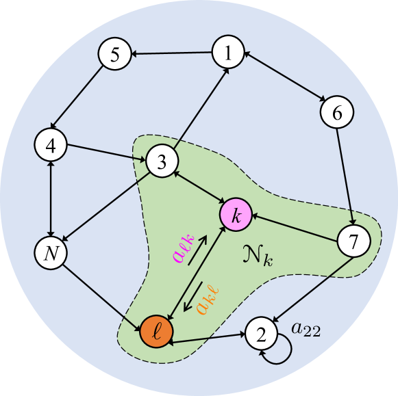
Figure 1: A strongly connected network consisting of $N$ agents. The neighborhood of agent $k$ is marked by the area highlighted in green.

The combination policy among agents is described by the matrix $A=[a_{\ell k}]$, where $a_{\ell k}$ is the weight that agent $k$ places on the information received from the neighboring agent $\ell$. We assume that the agents adopt a left-stochastic combination policy. Let $\mathcal{N}_{k}$ be the set of neighbors of agent $k$, then the combination matrix $A$ satisfies

$$A^{\top}\mathbbm{1}=\mathbbm{1},\quad a_{\ell k}>0,\;\;\forall\ell\in\mathcal{N}_{k},$$ (1)

and $a_{\ell k}=0$ for $\ell\notin\mathcal{N}_{k}$, where $\mathbbm{1}$ denotes the $N$-dimensional vector of all ones. The strong connectivity of the graph ensures that the combination matrix $A$ is primitive. According to the Perron-Frobenius theorem [25, 28], matrix $A$ has a single eigenvalue at $1$ and all other eigenvalues will be strictly inside the unit circle. Therefore, the second largest-magnitude eigenvalue of $A$ is strictly smaller than $1$. Moreover, the Perron eigenvector $\pi$ of matrix $A$ can be normalized to have strictly positive entries. That is,

$$A\pi=\pi,\quad\mathbbm{1}^{\top}\pi=1,\quad\pi_{k}>0,\;\;\forall k\in\mathcal{N}.$$ (2)

Observation model: At each time instant $i$, each agent $k$ receives a private signal $\bm{\xi}_{k,i}$ belonging to a certain space $\mathcal{X}_{k}$. Note that we are utilizing boldface notation to emphasize that $\bm{\xi}_{k,i}$ is random. The private signals of every agent, which are assumed to be statistically independent over time and space given a fixed true state of nature, are realizations of a random variable following an unknown distribution $f_{k}$:

$$\bm{\xi}_{k,i}\sim f_{k},\quad\forall k\in\mathcal{N}.$$ (3)

The joint observation profile at time instant $i$ generated by the network is denoted by $\bm{\xi}_{i}=(\bm{\xi}_{1,i},\bm{\xi}_{2,i},\dots,\bm{\xi}_{N,i})$, which is an i.i.d. sequence on the space $\mathcal{X}=\mathcal{X}_{1}\times\mathcal{X}_{2}\times\dots\times\mathcal{X}_{N}$ and distributed as $f=\prod_{k=1}^{N}f_{k}$ under the independence assumption of the private signals. Moreover, each agent $k$ has a family of local likelihood models $\{L_{k}(\cdot|\theta)\}$ parameterized by the hypothesis $\theta\in\Theta=\{\theta_{1},\theta_{2},\dots,\theta_{H}\}$. Among the given $H$ hypotheses, there is one true state of nature $\theta^{\star}\in\Theta$, referred to as the global truth for the network. Without loss of generality, we assume $\theta^{\star}=\theta_{1}$. In addition, we assume that $\{L_{k}(\cdot|\theta)\}$ has the same support as $f_{k}$, namely, $\mathcal{X}_{k}$. The likelihood of a signal ${\xi}$ received by agent $k$ conditioned on hypothesis $\theta$ is denoted by

$$L_{k}({\xi}|\theta),\quad\forall{\xi}\in\mathcal{X}_{k}.$$ (4)

Depending on whether the signal space $\mathcal{X}_{k}$ is continuous or discrete, the signal model $f_{k}$ and the likelihood models $\{L_{k}(\cdot|\theta)\}$ can be respectively probability density functions (pdfs) or probability mass functions (pmfs).

We consider a general learning scenario where the signal model $f_{k}$ may not match exactly any of the $H$ local likelihood models $L_{k}(\cdot|\theta)$. This is more general than many existing works (e.g., [3, 4, 5, 6, 11, 12, 14, 13]), where $f_{k}$ is taken as the likelihood model of the true hypothesis. That is, the signal $\bm{\xi}_{k,i}$ is a sample drawn according to the likelihood model $L_{k}(\cdot|\theta_{1})$:

$$\bm{\xi}_{k,i}\sim L_{k}(\cdot|\theta_{1}),\quad\forall k\in\mathcal{N}.$$ (5)

Since in this case all agents possess knowledge of the true signal model, we refer to scenario (5) as the accurate signal model scenario. In contrast, scenario (3) is referred to as the general signal model scenario. The Kullback-Leiber (KL) divergence [29] between $f_{k}$ and $L_{k}(\cdot|\theta)$, denoted by $D_{\textnormal{KL}}(f_{k}\|L_{k}(\cdot|\theta))$, is a useful measure of the “distance” between relevant distributions. Without loss of generality, we assume the following regularity condition on KL divergences [3, 4, 5, 6, 7, 8, 9, 10, 11, 12, 14, 13].

Assumption 2 (Finiteness of KL divergences).

For each hypothesis $\theta\in\Theta$ and for each agent $k\in\mathcal{N}$, $D_{\textnormal{KL}}(f_{k}\|L_{k}(\cdot|\theta))$ is finite. ∎

Two hypotheses $\theta_{m}$ and $\theta_{n}$ are said to be observationally equivalent from the perspective of agent $k$ if $D_{\textnormal{KL}}(f_{k}\|L_{k}(\cdot|\theta_{m}))=D_{\textnormal{KL}}(f_{k}\|L_{k}(\cdot|\theta_{n}))$. The optimal hypothesis set for agent $k$ (also called the local truth) is defined as the collection of hypotheses with the minimum KL divergence:

$$\Theta_{k}^{\star}\triangleq\operatorname*{argmin}_{\theta\in\Theta}D_{\textnormal{KL}}(f_{k}\|L_{k}(\cdot|\theta)).$$ (6)

Due to the non-negativeness of KL divergences, it is clear that in the accurate signal model scenario, the global truth $\theta_{1}$ is also a local truth for all agents, i.e., $\theta_{1}\in\Theta_{k}^{\star},\forall k\in\mathcal{N}$. However, in the general signal model scenario, some agents may fail to recognize the global truth due to the model discrepancy between $f_{k}$ and $L_{k}(\cdot|\theta_{1})$. We denote the sets of agents whose local truth agrees or collides with the global truth as $\mathcal{N}_{A}$ and $\overline{\mathcal{N}}_{A}$ respectively, such that $\mathcal{N}=\mathcal{N}_{A}\cup\overline{\mathcal{N}}_{A}$. The goal of all agents is to learn the global truth by cooperation with their neighbors. We note that we are not going to discuss the multi-task decision-making problem where different groups of agents in the network try to identify different hypotheses. The interested readers are referred to [24].

The optimal hypothesis set for the group $\mathcal{N}_{A}$ is defined as the common hypotheses shared by all agents $k\in\mathcal{N}_{A}$:

$$\Theta^{\star}=\bigcap_{k\in\mathcal{N}_{A}}{\Theta_{k}^{\star}}.$$ (7)

We impose the following identifiability assumption of the global truth on the group $\mathcal{N}_{A}$.

Assumption 3 (Identifiability).

Hypothesis $\theta_{1}$ is the unique optimal hypothesis for the group $\mathcal{N}_{A}$, i.e., $\Theta^{\star}=\left\{\theta_{1}\right\}$. ∎

For the accurate signal model (4)–(5), we have $\mathcal{N}_{A}=\mathcal{N}$, and thus Assumption 3 becomes the standard global identifiability assumption, namely, $\{\theta_{1}\}=\cap_{k=1}^{N}\Theta_{k}^{\star}$, as considered in [3, 4, 5, 6, 11, 12, 14, 13].

II-B Adaptive social learning strategy

We first introduce the basic framework of social learning.

Motivating example [7]: Consider a distributed source localization problem, where a network of $N$ agents receives noisy measurements of the distance to the source. Specifically, the private signal $\bm{\xi}_{k,i}$ received by agent $k$ at time instant $i$ is expressed as

$$\bm{\xi}_{k,i}={\sf d}_{k,i}+\bm{n}_{k,i}$$ (8)

where ${\sf d}_{k,i}$ denotes the distance between agent $k$ and the target measured at time instant $i$, and $\bm{n}_{k,i}$ is some zero-mean Gaussian noise. In the stationary environment where the target is assumed to be static, ${\sf d}_{k,i}$ is a constant for each agent $k$. The geographic region is partitioned into a collection of $H$ disjoint areas, and the hypothesis space $\Theta$ include all these possible locations. Each agent $k$ constructs likelihood functions $\{L_{k}(\cdot|\theta)\}$ based on its sensor model. In principle, each agent could estimate its distance to the target from its local observations. However, their information is not enough to arrive at the coordinates for the target, since each agent can only conclude that the target lies on a circle of radius ${\sf d}_{k,i}$ around it. To achieve the goal of source localization, the agents would need to cooperate with each other.

In social learning solutions, each agent $k$ holds a local belief vector $\bm{\mu}_{k,i}$ that represents a pmf over the set of hypotheses $\Theta$. Each component $\bm{\mu}_{k,i}(\theta)$ indicates the confidence of agent $k$ at time instant $i$ that $\theta$ is the true state of nature. In the context of source localization, $\bm{\mu}_{k,i}(\theta)$ denotes the agent $k$’s estimate of the probability that the target is located in area $\theta$. The belief vector is updated through the continuous flow of information in the network through an adaptation step and a combination step. More specifically, at each time instant $i$, agent $k$ receives a new signal $\bm{\xi}_{k,i}$ and uses it to compute an intermediate belief vector $\bm{\psi}_{k,i}$. In the non-adaptive learning scenario, the Bayes rule is employed, which computes $\bm{\psi}_{k,i}$ according to

$$\bm{\psi}_{k,i}(\theta)=\dfrac{\bm{\mu}_{k,i-1}(\theta)L_{k}(\bm{\xi}_{k,i}|\theta)}{\sum_{\theta^{\prime}\in\Theta}\bm{\mu}_{k,i-1}(\theta^{\prime})L_{k}(\bm{\xi}_{k,i}|\theta^{\prime})}$$ (9)

for each $\theta\in\Theta$. Eq. (9) describes how the agents refine their estimates of the target’s location with the latest measurement in the source localization example. After this adaptation step, agent $k$ aggregates the intermediate beliefs of its neighbors following a certain pooling protocol in order to update the local belief vector $\bm{\mu}_{k,i}$. Different protocols for belief aggregation lead to various social learning algorithms in the literature [3, 4, 5, 6, 7, 8, 9, 10, 11]. Examples of useful pooling rules appear in [30]. Next, we describe one fusion rule in the context of non-stationary environments.

First, we note that the ASL algorithm introduced in [12] is an important variant of social learning developed for non-stationary conditions. Within the previous distributed source localization example, the target might move to another location at some time instant $i_{0}$ and consequently, the distance ${\sf d}_{k,i}$ in (8) becomes a different value after $i\geq i_{0}$. It is necessary for the network to quickly track the new location of the target in practice. Adaptation is a desirable feature of distributed learning strategies [28, 25]. To improve the adaptation ability, a modified adaptive update (compared with (9)) is proposed in the ASL algorithm, where the weights assigned to the past and new information for constructing the intermediate belief are controlled through a small positive parameter $\delta$:

$$\bm{\psi}_{k,i}(\theta)=\dfrac{\bm{\mu}_{k,i-1}^{1-\delta}(\theta)L_{k}^{\delta}(\bm{\xi}_{k,i}|\theta)}{\sum_{\theta^{\prime}\in\Theta}\bm{\mu}_{k,i-1}^{1-\delta}(\theta^{\prime})L_{k}^{\delta}(\bm{\xi}_{k,i}|\theta^{\prime})}.$$ (10)

The motivation for this adaptation formula has been elaborated from different perspectives in [12]. In particular, we can get (10) as the solution to the following optimization problem:

$$\bm{\psi}_{k,i}=\operatorname*{argmin}_{p\in\Delta_{\theta}}\Big{\{}(1-\delta)D_{\textnormal{KL}}(p\|\bm{\mu}_{k,i-1})+\delta D_{\textnormal{KL}}(p\|\bm{\mu}_{k,i}^{\sf lik})\Big{\}}$$ (11)

where $\Delta_{\theta}$ is the set of all pmfs on the hypothesis set $\Theta$, and $\bm{\mu}_{k,i}^{\sf lik}$ is the likelihood pmf involving the new observation $\bm{\xi}_{k,i}$:

$$\bm{\mu}_{k,i}^{\sf lik}(\theta)=\frac{L_{k}(\bm{\xi}_{k,i}|\theta)}{\sum_{\theta^{\prime}\in\Theta}L_{k}(\bm{\xi}_{k,i}|\theta^{\prime})},\quad\forall\theta\in\Theta.$$ (12)

The first and second KL divergences in (11) describe respectively the consistency between the intermediate belief and the past information (captured by $\bm{\mu}_{k,i-1}$), and the consistency between the intermediate belief and the new information (represented by $\bm{\mu}_{k,i}^{\sf lik}$). The trade-off between these two consistency costs is adjusted through the parameter $\delta$. Following (10), the belief aggregation step employs the log-linear rule, which generates the local belief vector $\bm{\mu}_{k,i}$ as follows:

$$\bm{\mu}_{k,i}(\theta)=\dfrac{\exp{\sum_{\ell\in\mathcal{N}_{k}}a_{\ell k}\log{\bm{\psi}_{\ell,i}(\theta)}}}{\sum_{\theta^{\prime}\in\Theta}\exp{\sum_{\ell\in\mathcal{N}_{k}}a_{\ell k}\log{\bm{\psi}_{\ell,i}(\theta^{\prime})}}}$$ (13)

for each $\theta\in\Theta$. This pooling rule (13) can be obtained as the solution to the following optimization problem:

$$\bm{\mu}_{k,i}=\operatorname*{argmin}_{p\in\Delta_{\theta}}\Bigg{\{}\sum_{\ell=1}^{N}a_{\ell k}D_{\textnormal{KL}}(p\|\bm{\psi}_{\ell,i})\Bigg{\}}.$$ (14)

Since its inception, the ASL algorithm has been applied to different tasks, such as discovering influencers in opinion formation over online social networks [31] and solving image classification problems involving heterogeneous classifiers [32].

To avoid trivial cases, we assume that for all agents, the initial belief on each hypothesis $\theta\in\Theta$ is non-zero, i.e., $\bm{\mu}_{k,0}(\theta)>0,\forall k\in\mathcal{N}$. This is because if $\bm{\mu}_{\ell,0}(\theta)=0$ for some $\ell\in\mathcal{N}$ and $\theta\in\Theta$, then from (10) and (13), we have $\bm{\mu}_{k,N-1}(\theta)=0$ for all agents due to Assumption 1. Hence, hypothesis $\theta$ will end up being excluded from the social learning process.

Assumption 4 (Positive initial belief).

For each hypothesis $\theta\in\Theta$ and for each agent $k\in\mathcal{N}$, the initial belief $\bm{\mu}_{k,0}(\theta)$ is positive. ∎

Under Assumptions 1–4, we discuss the steady-state learning performance of the ASL strategy for the general signal model (3)–(4).

II-C Steady-state learning performance

We start by introducing the log-belief ratios $\bm{\nu}_{k,i}(\theta)$ and $\bm{\lambda}_{k,i}(\theta)$ for all $k\in\mathcal{N}$ and $\theta\in\Theta$:

$$\bm{\nu}_{k,i}(\theta)\triangleq\log\frac{\bm{\psi}_{k,i}(\theta_{1})}{\bm{\psi}_{k,i}(\theta)},\quad\bm{\lambda}_{k,i}(\theta)\triangleq\log{\frac{\bm{\mu}_{k,i}(\theta_{1})}{\bm{\mu}_{k,i}(\theta)}}.$$ (15)

Each agent makes a decision about the underlying state based on its belief. One natural option is to select the hypothesis that maximizes the belief. For each agent $k\in\mathcal{N}$, the instantaneous error probability of social learning at time instant $i$ is defined as

$$p_{k,i}\triangleq\mathbb{P}\Big{[}\operatorname*{argmax}_{\theta\in\Theta}\bm{\mu}_{k,i}(\theta)\neq\theta_{1}\Big{]}=\mathbb{P}\Big{[}\exists\theta\neq\theta_{1}:\bm{\lambda}_{k,i}(\theta)\leq 0\Big{]}.$$ (16)

We also introduce the log-likelihood ratio $\bm{x}_{k,i}(\theta)$ for all $k\in\mathcal{N}$ and $\theta\in\Theta$:

$$\bm{x}_{k,i}(\theta)\triangleq\log{\frac{L_{k}(\bm{\xi}_{k,i}|\theta_{1})}{L_{k}(\bm{\xi}_{k,i}|\theta)}}.$$ (17)

Using the variables $\bm{\nu}_{k,i}(\theta)$, $\bm{\lambda}_{k,i}(\theta)$ and $\bm{x}_{k,i}(\theta)$ in the logarithmic domain, the ASL algorithm represented by (10) and (13) can be rewritten as a two-step linear recursion:

$$\begin{cases}\bm{\nu}_{k,i}(\theta)=(1-\delta)\bm{\lambda}_{k,i-1}(\theta)+\delta\bm{x}_{k,i}(\theta)\\[3.0pt] \bm{\lambda}_{k,i}(\theta)=\sum\limits_{\ell\in\mathcal{N}_{k}}a_{\ell k}\bm{\nu}_{\ell,i}(\theta)\end{cases}$$ (18)

which has the form of a standard diffusion learning rule [25, 28]. Iterating the recursion in (18), we obtain

$$\bm{\lambda}_{k,i}(\theta)= \;(1-\delta)^{i}\sum_{\ell=1}^{N}[A^{i}]_{\ell k}\bm{\lambda}_{\ell,0}(\theta)$$

$$+\delta\sum_{m=0}^{i-1}\sum_{\ell=1}^{N}(1-\delta)^{m}[A^{m+1}]_{\ell k}\bm{x}_{\ell,i-m}(\theta).$$ (19)

The first term in (19) involves the initial belief vector and it decays as $i$ grows. In order to evaluate the steady-state learning performance, it suffices to focus on the second term:

$$\widehat{\bm{\lambda}}_{k,i}(\theta)\triangleq\delta\sum_{m=0}^{i-1}\sum_{\ell=1}^{N}(1-\delta)^{m}[A^{m+1}]_{\ell k}\bm{x}_{\ell,i-m}(\theta).$$ (20)

Given that the random variables $\bm{x}_{k,i}(\theta)$ are i.i.d. across time, and that our analysis concerns only the distribution of partial sums associated with these terms, it is useful to introduce the following random variable:

$$\widetilde{\bm{\lambda}}_{k,i}(\theta)\triangleq\delta\sum_{m=0}^{i-1}\sum_{\ell=1}^{N}(1-\delta)^{m}[A^{m+1}]_{\ell k}\bm{x}_{\ell,m+1}(\theta)$$ (21)

where the summation in (20) is taken in reversed order. By repeating the same arguments used in [22, 23, 12], we can show that $\widehat{\bm{\lambda}}_{k,i}(\theta)$ and $\widetilde{\bm{\lambda}}_{k,i}(\theta)$ share the same distribution. Formally,

$$\widehat{\bm{\lambda}}_{k,i}(\theta)\overset{\textnormal{d}}{=}\widetilde{\bm{\lambda}}_{k,i}(\theta)$$ (22)

where the symbol $\overset{\textnormal{d}}{=}$ denotes equality in distribution. Furthermore, the random variable $\widetilde{\bm{\lambda}}_{k,i}(\theta)$ converges almost surely as $i\to\infty$ under Assumptions 1–2. Therefore, there exists a steady-state random variable termed as steady-state log-belief ratio:

$$\widetilde{\bm{\lambda}}_{k,\infty}(\theta)\triangleq\delta\sum_{m=0}^{\infty}\sum_{\ell=1}^{N}(1-\delta)^{m}[A^{m+1}]_{\ell k}\bm{x}_{\ell,m+1}(\theta)$$ (23)

such that

$$\widehat{\bm{\lambda}}_{k,i}(\theta)\overset{i\to\infty}{\rightsquigarrow}\widetilde{\bm{\lambda}}_{k,\infty}(\theta)$$ (24)

where the symbol $\rightsquigarrow$ means convergence in distribution. In view of (16), the relation in (24) allows us to define the steady-state error probability for each agent $k$ as:

$$p_{k}\triangleq\mathbb{P}\big{[}\exists\theta\neq\theta_{1}:\widetilde{\bm{\lambda}}_{k,\infty}(\theta)\leq 0\big{]}.$$ (25)

Using similar analytical tools to the ones employed in [12], we can prove that for small $\delta$, the steady-state error probability $p_{k}$ obeys a Large Deviations Principle (LDP) [33, 34] for some error exponent that is related to the combination policy. For the benefit of the reader, we recall here that a process $\bm{y}_{\delta}$ is said to obey an LDP if the following limit exists [33, 34]:

$$\underset{\delta\to 0}{\lim\;}\delta\ln\mathbb{P}\big{[}\bm{y}_{\delta}\in\Gamma\big{]}=-\underset{\gamma\in\Gamma}{\inf}I(\gamma)\triangleq-I_{\Gamma}$$ (26)

for some $I(\gamma)$ that is called the rate function, where $\Gamma$ is an arbitrary set. Equivalently,

$$\mathbb{P}\left[\bm{y}_{\delta}\in\Gamma\right]\doteq e^{-(1/\delta)I_{\Gamma}}$$ (27)

where the symbol $\doteq$ denotes equality to the leading order in the exponent as $\delta$ goes to zero. For the social learning problem, the leading-order exponent $I_{\Gamma}$ corresponding to the error probability is also referred to as error exponent.

For our subsequent analysis on the error exponent, we also need to introduce the network average log-likelihood ratio for all $\theta\in\Theta$:

$$\bm{x}_{{\sf ave},i}(\pi,\theta)\triangleq\sum_{k=1}^{N}{\pi_{k}\bm{x}_{k,i}(\theta)}.$$ (28)

We note that the combination policy, which is the main subject of interest in this work, plays a key role in weighting the network average quantity defined above. Let $\mathbb{E}$ and $\mathbb{P}$ denote the expectation and probability operators relative to the joint signal model $f$, respectively. The expectation of $\bm{x}_{k,i}(\theta)$ is given by

$$d_{k}(\theta)\triangleq\mathbb{E}\left[{\bm{x}}_{k,i}(\theta)\right]=D_{\textnormal{KL}}({f_{k}}\|L_{k}(\cdot|\theta))-D_{\textnormal{KL}}({f_{k}}\|L_{k}(\cdot|\theta_{1})).$$ (29)

Assumption 2 ensures that $d_{k}(\theta)$ is finite, i.e., $\absolutevalue{d_{k}(\theta)}<\infty$ for all $k\in\mathcal{N}$ and for all $\theta\in\Theta$. By definition (6), we know that if $d_{k}(\theta)\geq 0$ for all $\theta\neq\theta_{1}$, then the global truth $\theta_{1}$ is also a local truth for agent $k$, i.e., $\theta_{1}\in\Theta_{k}^{\star}$. Otherwise, it conflicts with the local truth at agent $k$, i.e., $\theta_{1}\notin\Theta_{k}^{\star}$. From (28), the expectation of $\bm{x}_{{\sf ave},i}(\pi,\theta)$ can be written as

$${\sf m_{ave}}(\pi,\theta)\triangleq\mathbb{E}\left[\bm{x}_{{\sf ave},i}(\pi,\theta)\right]=\sum_{k=1}^{N}{\pi_{k}d_{k}(\theta)}.$$ (30)

Let $\Lambda_{k}(t;\theta)$ and $\Lambda_{\sf ave}(t;\pi,\theta)$ denote the Logarithmic Moment Generating Functions (LMGFs) of variables $\bm{x}_{k,i}(\theta)$ and $\bm{x}_{{\sf ave},i}(\pi,\theta)$, respectively:

$$\Lambda_{k}(t;\theta)\triangleq\log\mathbb{E}\Big{[}e^{t\bm{x}_{k,i}(\theta)}\Big{]},$$ (31)

$$\Lambda_{\sf ave}(t;\pi,\theta)\triangleq\log\mathbb{E}\Big{[}e^{t\bm{x}_{{\sf ave},i}(\pi,\theta)}\Big{]}=\sum_{k=1}^{N}\Lambda_{k}(\pi_{k}t;\theta).$$ (32)

We note that since the random variables $\bm{x}_{k,i}(\theta)$ are i.i.d. across time, $\Lambda_{k}(t;\theta)$ and $\Lambda_{\sf ave}(t;\pi,\theta)$ are independent of time. For this reason, the subscript $i$ pertaining to the time instant is not required. One fundamental property of LMGFs states that $\Lambda_{k}(t;\theta)$ is an alternative representation for the probability distribution of $\bm{x}_{k,i}(\theta)$. Hence, it captures the informativeness of agent $k$ on learning the global truth $\theta_{1}$.

In the following theorem, we extend two important results on the steady-state learning performance in the small-$\delta$ regime to the general signal model; these results were previously established, albeit only for the accurate signal model in [12].

Theorem 1 (Steady-state learning performance).

Under Assumptions 1–4 for the general signal model (3)–(4), we consider a combination policy with Perron eigenvector $\pi$. In the small-$\delta$ regime, the steady-state log-belief ratio $\widetilde{\bm{\lambda}}_{k,\infty}(\theta)$ converges to ${\sf m_{ave}}(\pi,\theta)$ in probability as $\delta$ approaches 0:

$$\widetilde{\bm{\lambda}}_{k,\infty}(\theta)\xrightarrow{\delta\to 0}{\sf m_{ave}}(\pi,\theta)\quad\textnormal{in probability}$$ (33)

for all $\theta\in\Theta$. Therefore, if the Perron eigenvector $\pi$ satisfies

$${\sf m_{ave}}(\pi,\theta)>0,\quad\forall\theta\neq\theta_{1},$$ (34)

we have:

1. Consistency of learning: The steady-state error probability $p_{k}$ converges to 0 as $\delta$ goes to 0 by definition (25). This means that all agents learn the global truth successfully.

2. Error exponent: Assume $\Lambda_{k}(t;\theta)<\infty,\forall t\in\mathbb{R}$ for all $k\in\mathcal{N}$ and $\theta\neq\theta_{1}$. The steady-state error probability $p_{k}$ obeys an LDP with rate $\frac{1}{\delta}$ and error exponent $\Phi(\pi)$, i.e.,

   $$p_{k}\doteq e^{-\Phi(\pi)/\delta},$$ (35)

   where

   $$\Phi(\pi)\triangleq\min_{\theta\neq\theta_{1}}\Phi(\pi,\theta).$$ (36)

   The $\theta$-related error exponent $\Phi(\pi,\theta)$ is given by

   $$\Phi(\pi,\theta)\triangleq-\inf_{t\in\mathbb{R}}\phi(t;\pi,\theta)$$ (37)

   with

   $$\phi(t;\pi,\theta)\triangleq\int_{0}^{t}\frac{\Lambda_{\sf ave}(\tau;\pi,\theta)}{\tau}d\tau.$$ (38)

Proof.

The performance analysis on the ASL strategy for the accurate signal model (4)–(5) has been established in [12]. From the analysis there, the steady-state learning performance is determined by the statistical properties of the log-likelihood ratio involving the true hypothesis and an alternative one. We note that there are some differences in notation between [12] and this work. For instance, the $H$ hypotheses are numbered from $0$ to $H-1$, and the true state is denoted by $\theta_{0}$ in [12]. Using the notation introduced in this paper, the key condition to the proof in [12] is that the log-likelihood ratio $\bm{x}_{k,i}(\theta)$ has a finite mean for all $k\in\mathcal{N}$ and $\theta\in\Theta$ (see Lemma 1 in [12]). That is,

$$\mathbb{E}\big{[}\bm{x}_{k,i}(\theta)\big{]}\triangleq\mathbb{E}_{L_{k}(\cdot|\theta_{1})}\big{[}\bm{x}_{k,i}(\theta)\big{]}<\infty,$$ (39)

which is ensured by the assumption of finite KL divergences (i.e., Assumption 1 in [12]). The only difference in the analysis for a general signal model (3)–(4) is that, we need to examine the statistical properties of $\bm{x}_{k,i}(\theta)$ conditioned on a general model $f_{k}$ which might be different from the likelihood model $L_{k}(\cdot|\theta_{1})$. However, under Assumption 2, we have $\mathbb{E}[\bm{x}_{k,i}(\theta)]<\infty$ as shown in (29). Therefore, the finite-mean condition (39) continues to hold for the general signal model:

$$\mathbb{E}\big{[}\bm{x}_{k,i}(\theta)\big{]}\triangleq\mathbb{E}_{f_{k}}\big{[}\bm{x}_{k,i}(\theta)\big{]}<\infty.$$ (40)

Consequently, Theorem 1 is established by repeating the proof of the steady-state learning performance developed in [12] by substituting the expectation w.r.t. $L_{k}(\cdot|\theta_{1})$ by that w.r.t. $f_{k}$. ∎

III Maximizing error exponent

In this section, we discuss the effect of combination policies on the steady-state learning accuracy of the ASL strategy. From Theorem 1, the error exponent $\Phi(\pi)$ plays a crucial role in the steady-state error probability. According to (36)–(38), $\Phi(\pi)$ is influenced by the Perron eigenvector of the combination policy through the LMGF $\Lambda_{\sf ave}(t;\pi,\theta)$ defined in (32). A Perron eigenvector that delivers a larger error exponent is beneficial for reducing the steady-state error probability in the slow adaptation regime. To find the best Perron eigenvectors that provide the largest error exponent for the given learning task, we formulate the following optimization problem:

$$\max_{\pi}\;\Phi(\pi)$$ (41)

s.t. $$\mathbbm{1}^{\top}\pi=1,\;\pi_{k}>0,\quad\forall k\in\mathcal{N},$$ (42)

$${\sf m_{ave}}(\pi,\theta)>0,\qquad\;\forall\theta\neq\theta_{1}.$$ (43)

Here, constraints (42) and (43) are imposed to guarantee the strong connectivity of the network and the successful learning of the global truth according to Theorem 1. We denote the set of all feasible solutions to the optimization problem (41)–(43) by $\Pi$:

$$\Pi=\left\{\pi:\pi\text{ satisfies }\eqref{eq: constraint 1}\text{ and }\eqref{eq: constraint 2}\right\}.$$ (44)

It is clear from (36)–(38) that the design of $\pi$ relates to the individual LMGFs $\Lambda_{k}(t;\theta)$, which measure the ability of every agent $k$ to learn the global truth $\theta_{1}$, namely, its level of informativeness. Before solving the optimization problem above, we first provide some useful definitions and preliminary results for the subsequent analysis.

III-A Preliminary definitions

We classify the $N$ agents into different groups according to their informativeness. Agents in different groups play different roles in the learning performance. For each wrong hypothesis $\theta\neq\theta_{1}$, we denote the sets $\mathcal{N}^{{U}}(\theta)$, $\mathcal{N}^{{I}}(\theta)$, and $\mathcal{N}^{{C}}(\theta)$ as the collections of uninformative agents, informative agents and conflicting agents with respect to $\theta$, respectively:

$$\mathcal{N}^{{U}}(\theta)\triangleq \left\{k\in\mathcal{N}:\Lambda_{k}(t;\theta)\equiv 0\right\},$$ (45)

$$\mathcal{N}^{{I}}(\theta)\triangleq \left\{k\in\mathcal{N}:\Lambda_{k}(t;\theta)\not\equiv 0,d_{k}(\theta)>0\right\},$$ (46)

$$\mathcal{N}^{{C}}(\theta)\triangleq \left\{k\in\mathcal{N}:\Lambda_{k}(t;\theta)\not\equiv 0,d_{k}(\theta)\leq 0\right\},$$ (47)

where the symbol $\equiv$ denotes that $\Lambda_{k}(t;\theta)=0$ for all $t\in\mathbb{R}$, and the symbol $\not\equiv$ means that $\Lambda_{k}(t;\theta)\neq 0$ for some $t\in\mathbb{R}$. According to the definitions above, an agent $k$ is $\theta$-uninformative if the likelihoods conditioned on hypotheses $\theta_{1}$ and $\theta$ are the same for all local observations (i.e., $L_{k}(\cdot|\theta)=L_{k}(\cdot|\theta_{1})$ almost everywhere), and is $\theta$-informative if hypothesis $\theta_{1}$ is more consistent with its local observations than hypothesis $\theta$. It is $\theta$-conflicting if its information associated to hypothesis $\theta$ is detrimental for learning the global truth $\theta_{1}$. This point will be self-evident later when we discuss the bounds of error exponents. Moreover, it is clear that if $k\in\overline{\mathcal{N}}_{A}$ (i.e., $\theta_{1}\not\in\Theta_{k}^{\star}$), then agent $k$ must be a conflicting agent for some hypothesis $\theta$. Another observation is that definition (45) of a $\theta$-uninformative agent $k$ requires a more stringent condition (i.e., $\Lambda_{k}(t;\theta)\equiv 0$) than the observational equivalence of $\theta_{1}$ and $\theta$ from the perspective of agent $k$ (i.e., $d_{k}(\theta)=0$). In particular, due to the non-negativeness of KL divergence, $\Lambda_{k}(t;\theta)\equiv 0$ implies that $d_{k}(\theta)=0$ under the accurate signal model (4)–(5). We provide the following example to illustrate the aforementioned sets of agents.

Example: Consider a network of 4 sensor agents tasked with a binary detection problem. In practice, the likelihood models are usually constructed from a finite number of samples collected under the corresponding hypothesis. Assume that the signal model is $f_{k}={\sf N}(0,1)$ for all agents, where ${\sf N}(a,b)$ denotes the Gaussian pdf with mean $a$ and variance $b$. Due to the limited number of samples, the likelihood models might be inaccurate and thus differ from the underlying signal model. Let us consider a group of unit-variance Gaussian likelihood models: $L_{k}(\cdot|\theta_{1})={\sf N}(0.1,1)$ for all $k$, and

$$L_{1}(\cdot|\theta_{2})={\sf N}(-0.1,1), L_{2}(\cdot|\theta_{2})={\sf N}(0.2,1),$$ (48)

$$L_{3}(\cdot|\theta_{2})={\sf N}(0,1), L_{4}(\cdot|\theta_{2})={\sf N}(0.1,1).$$ (49)

Under the ASL protocol, the expectations $d_{k}(\theta_{2})$ are given by $d_{1}(\theta_{2})=d_{4}(\theta_{2})=0$, $d_{2}(\theta_{2})=0.03$ and $d_{3}(\theta_{2})=-0.01$. The LMGFs $\Lambda_{k}(t;\theta_{2})$ for all $k\in\mathcal{N}$ are presented in Fig. 2. According to definitions (45)–(47), we have $\mathcal{N}^{U}(\theta_{2})=\{4\}$, $\mathcal{N}^{I}(\theta_{2})=\{2\}$ and $\mathcal{N}^{C}(\theta_{2})=\{1,3\}$. Therefore, the learning performance of this network will be affected by the eigenvector centrality of different types of agents. ∎

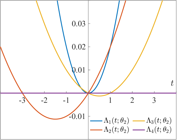
Figure 2: LMGFs $\Lambda_{k}(t;\theta_{2})$ for $k\in\mathcal{N}$ in the example.

Next, we introduce two important quantities related to the learning performance in the non-cooperative scenario, where the ASL algorithm update (18) at agent $k$ becomes

$$\bm{\lambda}^{\sf nc}_{k,i}(\theta)=\bm{\nu}^{\sf nc}_{k,i}(\theta)=(1-\delta)\bm{\lambda}^{\sf nc}_{k,i-1}(\theta)+\delta\bm{x}_{k,i}(\theta).$$ (50)

Here and in the following, we use the superscript ‘$\sf nc$’ for variables associated with the non-cooperative scenario. Similar to (23) in the social learning setting, we introduce the steady-state log-belief ratio for agent $k$:

$$\widetilde{\bm{\lambda}}_{k,\infty}^{\sf nc}(\theta)\triangleq\delta\sum_{m=0}^{\infty}(1-\delta)^{m}\bm{x}_{k,m+1}(\theta).$$ (51)

Accordingly, we define the $\theta$-related steady-state error probability as

$$p_{k}^{\sf nc}(\theta)\triangleq\mathbb{P}[\widetilde{\bm{\lambda}}_{k,\infty}^{\sf nc}(\theta)\leq 0].$$ (52)

Let $\Phi_{k}^{\sf nc}(\theta)$ denote the $\theta$-related error exponent for agent $k$ in this single-agent setup for each $\theta\neq\theta_{1}$:

$$p_{k}^{\sf nc}(\theta)\doteq e^{-\Phi_{k}^{\sf nc}(\theta)/\delta}.$$ (53)

It is clear that $\Phi_{k}^{\sf nc}(\theta)\geq 0$ for all $k\in\mathcal{N}$. Similar to (38), we define the function $\phi_{k}^{\sf nc}(t;\theta)$:

$$\phi_{k}^{\sf nc}(t;\theta)\triangleq\int_{0}^{t}\frac{\Lambda_{k}(\tau;\theta)}{\tau}d\tau.$$ (54)

Let $t_{k}^{\sf nc}(\theta)\leq 0$ be the critical value to attain $\Phi_{k}^{\sf nc}(\theta)$ for each agent $k\in\mathcal{N}$:

$$\Phi_{k}^{\sf nc}(\theta)=-\phi_{k}^{\sf nc}(t_{k}^{\sf nc}(\theta);\theta).$$ (55)

We will show that $t_{k}^{\sf nc}(\theta)$ is essential to characterize the optimal solution of the error exponent maximization problem (41)–(43). The value of $t_{k}^{\sf nc}(\theta)$ for agent $k$ in different groups $\mathcal{N}^{I}(\theta)$, $\mathcal{N}^{U}(\theta)$ and $\mathcal{N}^{C}(\theta)$ is derived as follows.

For each $\theta$-informative agent $k\in\mathcal{N}^{{I}}(\theta)$, $\Phi_{k}^{\sf nc}(\theta)$ can be expressed as

$$\Phi_{k}^{\sf nc}(\theta)=-\inf_{t\in\mathbb{R}}\phi_{k}^{\sf nc}(t;\theta)$$ (56)

by using the results from Theorem 1. With the properties of $\Lambda_{k}(t;\theta)$ and $\phi_{k}^{\sf nc}(t;\theta)$ established in Lemma 1 (Appendix A), we have $\Phi_{k}^{\sf nc}(\theta)>0$. The existence and uniqueness of $t_{k}^{\sf nc}(\theta)$ for each $\theta$-informative agent is proved in Appendix B. If agent $k$ is $\theta$-uninformative, we have $\Lambda_{k}(t;\theta)\equiv 0$ from (45). Hence, we obtain $\Phi_{k}^{\sf nc}(\theta)=0$ and $t_{k}^{\sf nc}(\theta)$ can be any non-positive value. We assume $t_{k}^{\sf nc}(\theta)=-C$ for simplicity, where $C$ is an arbitrary positive constant that can be dependent on $k$ and $\theta$. In addition, if agent $k$ is $\theta$-conflicting, then as $\delta$ approaches 0, it rejects hypothesis $\theta_{1}$ (if $d_{k}(\theta)<0$) or cannot distinguish between hypotheses $\theta_{1}$ and $\theta$ (if $d_{k}(\theta)=0$) with probability $1$ in steady state. From (53), $\Phi_{k}^{\sf nc}(\theta)=0$ is obtained in this case. Moreover, according to Lemma 1 in Appendix A, the following condition holds for any $\theta$-conflicting agent $k$:

$$\phi_{k}^{\sf nc}(t;\theta)>0,\quad\forall t<0,$$ (57)

which yields $t_{k}^{\sf nc}(\theta)=0$ in (55). Based on the above analysis, we obtain

$$t_{k}^{\sf nc}(\theta):\begin{cases}<0,&\text{if }k\in\mathcal{N}^{I}(\theta),\\ =-C,&\text{if }k\in\mathcal{N}^{U}(\theta),\\ =0,&\text{if }k\in\mathcal{N}^{C}(\theta).\end{cases}$$ (58)

Consider the previous example with LMGFs shown in Fig. 2. We have $t_{2}^{\sf nc}(\theta_{2})=-3$ and $t_{1}^{\sf nc}(\theta_{2})=t_{3}^{\sf nc}(\theta_{2})=0$. Since agent $4$ is $\theta_{2}$-uninformative, $t_{4}^{\sf nc}(\theta_{2})$ can take arbitrary value $-C$.

III-B General results

Let $\Phi_{{\sum}}^{\sf nc}(\theta)$ denote the sum of individual $\Phi_{k}^{\sf nc}(\theta)$ in the non-cooperative scenario:

$$\Phi_{\sum}^{\sf nc}(\theta)\triangleq\sum_{k=1}^{N}\Phi_{k}^{\sf nc}(\theta).$$ (59)

Then, we can derive the following bound for the error exponent $\Phi(\pi)$ for any feasible Perron eigenvector $\pi\in\Pi$.

Theorem 2 (Benefit of cooperation).

For any Perron eigenvector $\pi\in\Pi$, the $\theta$-related error exponent $\Phi(\pi,\theta)$ defined in (37) is bounded by

$$\min_{k\in\mathcal{N}}\Phi^{\sf nc}_{k}(\theta)\leq\Phi(\pi,\theta)\leq\Phi_{\sum}^{\sf nc}(\theta),\quad\forall\theta\neq\theta_{1}.$$ (60)

Correspondingly, the error exponent $\Phi(\pi)$ of the steady-state error probability is bounded by

$$\min_{\theta\neq\theta_{1}}\min_{k\in\mathcal{N}}\Phi^{\sf nc}_{k}(\theta)\leq\Phi(\pi)\leq\min_{\theta\neq\theta_{1}}\Phi_{\sum}^{\sf nc}(\theta).$$ (61)

Proof.

See Appendix B. ∎

Theorem 2 shows that the error exponent under adaptive social learning is no less than the worst error exponent in the single-agent setup. Therefore, the cooperation among agents is always beneficial for the agent that has the worst learning performance in the non-cooperative scenario. In addition, the best error exponent that can be achieved by the ASL strategy is given by the minimum aggregated quantity $\Phi_{\sum}^{\sf nc}(\theta)$ among all wrong hypotheses $\theta\neq\theta_{1}$. Since the centralized solution of the adaptive social learning problem is equivalent to a fully connected network, (61) applies to the centralized case as well. Furthermore, the upper bound in (61) satisfies

$$\min_{\theta\neq\theta_{1}}{\Phi}^{\sf nc}_{\sum}(\theta)\triangleq\min_{\theta\neq\theta_{1}}\sum_{k=1}^{N}{\Phi}^{\sf nc}_{k}(\theta)\geq\sum_{k=1}^{N}\min_{\theta\neq\theta_{1}}{\Phi}^{\sf nc}_{k}(\theta),$$ (62)

which reveals that the cooperation among agents enables each agent in the network to obtain an error exponent that could be even larger than the sum of individual error exponents in the non-cooperative scenario. However, the achievability of the upper bound in (61) is related to the specific setting of learning tasks. For instance, the existence of some conflicting agents may lead to a smaller error exponent. We will describe next when this upper bound is achievable and how to reach this upper bound with proper combination policies.

Let $\theta^{\dagger}$ be the wrong hypothesis corresponding to the upper bound in (61):

$$\theta^{\dagger}\triangleq\operatorname*{argmin}_{\theta\neq\theta_{1}}\Phi_{\sum}^{\sf nc}(\theta).$$ (63)

From Theorem 2, we have $\Phi(\pi)\leq\Phi_{\sum}^{\sf nc}(\theta^{\dagger})$ for all Perron eigenvectors $\pi\in\Pi$. Therefore, any Perron eigenvector $\pi\in\Pi$ that gives $\Phi(\pi)=\Phi_{\sum}^{\sf nc}(\theta^{\dagger})$ must be an optimal solution to the optimization problem in (41)–(43). In view of constraint (43), ${\sf m_{ave}}(\pi,\theta^{\dagger})>0$ for any $\pi\in\Pi$. Then, we have

$$\Phi(\pi,\theta^{\dagger})\overset{\eqref{eq: rate function}}{=}-\inf_{t\in\mathbb{R}}\phi(t;\pi,\theta^{\dagger})=-\phi(t^{\ast}_{\pi};\pi,\theta^{\dagger})$$ (64)

for some $t^{\ast}_{\pi}<0$ due to properties v) and vi) in Lemma 1. By definitions (32), (38), and (54), the following inequality holds:

$$\Phi(\pi,\theta^{\dagger}) =-\sum_{k\in\mathcal{N}^{C}(\theta^{\dagger})}{\phi_{k}^{\sf nc}(\pi_{k}t^{\ast}_{\pi};\theta)}-\sum_{k\notin\mathcal{N}^{C}(\theta^{\dagger})}\phi_{k}^{\sf nc}(\pi_{k}t^{\ast}_{\pi};\theta)$$

$${\leq}-\sum_{k\notin\mathcal{N}^{C}(\theta^{\dagger})}\phi_{k}^{\sf nc}(\pi_{k}t^{\ast}_{\pi};\theta)\overset{\eqref{eq: error exponent individually}}{\leq}\Phi_{\sum}^{\sf nc}(\theta^{\dagger}).$$ (65)

Due to the constraint $\pi_{k}>0,\forall k\in\mathcal{N}$ in (42), the first inequality in (65) becomes equality if and only if $\mathcal{N}^{C}(\theta^{\dagger})=\emptyset$. Hence, the upper bound in (61) cannot be attained if there are some $\theta^{\dagger}$-conflicting agents in the network. Eqs. (57) and (65) illustrate our definition (47) of the $\theta$-conflicting agents. In the following, we discuss the design of optimal Perron eigenvectors for the cases $\mathcal{N}^{C}(\theta^{\dagger})=\emptyset$ and $\mathcal{N}^{C}(\theta^{\dagger})\neq\emptyset$, respectively.

III-B1 Case 1: $\mathcal{N}^{C}(\theta^{\dagger})=\emptyset$

In this case, the quantity $t_{k}^{\sf nc}(\theta^{\dagger})$ defined in (58) is negative for all $k\in\mathcal{N}$. With this property, we construct the following candidate Perron eigenvector $\pi^{\dagger}$:

$$\pi_{k}^{\dagger}=\frac{t_{k}^{\sf nc}(\theta^{\dagger})}{\sum_{\ell=1}^{N}t_{\ell}^{\sf nc}(\theta^{\dagger})},\quad\forall k\in\mathcal{N}.$$ (66)

It is easy to see that $\mathbbm{1}^{\top}\pi^{\dagger}=1$ and $\pi^{\dagger}_{k}>0,\forall k\in\mathcal{N}$. Under Perron eigenvector $\pi^{\dagger}$, the $\theta^{\dagger}$-related error exponent $\Phi(\pi^{\dagger},\theta^{\dagger})$ equals to the upper bound in (61):

$$\Phi_{\sum}^{\sf nc}(\theta^{\dagger})\overset{\eqref{eq: bound of each error exponent}}{\geq}\Phi(\pi^{\dagger},\theta^{\dagger}) {=}-\inf_{t\in\mathbb{R}}\phi(t;\pi^{\dagger},\theta^{\dagger})$$

$$\geq-\phi\left({\sum\limits_{k=1}^{N}t_{k}^{\sf nc}({\theta^{\dagger}})};\pi^{\dagger},\theta^{\dagger}\right)$$

$${=}-\sum_{k=1}^{N}\phi_{k}^{\sf nc}({t_{k}^{\sf nc}(\theta^{\dagger})};\theta^{\dagger})$$

$${=}\sum_{k=1}^{N}\Phi_{k}^{\sf nc}(\theta^{\dagger})\triangleq\Phi_{\sum}^{\sf nc}(\theta^{\dagger})$$ (67)

where in (a) we used the definitions given in (32), (38), (54), and (66). From Theorem 1, the error exponent $\Phi(\pi^{\dagger})$ under Perron eigenvector $\pi^{\dagger}$ is determined by the minimum $\theta$-related error exponent $\Phi(\pi^{\dagger},\theta)$. If $\pi^{\dagger}$ is feasible for the truth learning (i.e., $\pi^{\dagger}\in\Pi$) and satisfies $\Phi(\pi^{\dagger},\theta^{\dagger})\leq\Phi(\pi^{\dagger},\theta)$, $\forall\theta\neq\theta_{1}$, then we have

$$\Phi(\pi^{\dagger})\triangleq\min_{\theta\neq\theta_{1}}\Phi(\pi^{\dagger},\theta)=\Phi(\pi^{\dagger},\theta^{\dagger})\overset{\eqref{eq: pi_dagger for the upper bound-case 1}}{=}\Phi_{\sum}^{\sf nc}(\theta^{\dagger}),$$ (68)

which proves that $\pi^{\dagger}$ is an optimal solution. Let $\Pi_{1}$ denote the following set of Perron eigenvectors:

$$\Pi_{1}=\Big{\{}\pi\in\Pi:\Phi(\pi,\theta^{\dagger})\leq\Phi(\pi,\theta),\forall\theta\neq\theta_{1}\Big{\}}.$$ (69)

In the following theorem, we formally establish the achievability of the upper bound in (61) for the error exponent maximization problem in (41)–(43), and characterize the optimal Perron eigenvectors corresponding to this upper bound.

Theorem 3a (Optimal Perron eigenvector).

Consider $\mathcal{N}^{C}(\theta^{\dagger})=\emptyset$. Let $\Phi^{\star}$ be the maximum error exponent in the optimization problem (41)–(43) and $\Pi^{\star}$ be the set of optimal Perron eigenvectors. Define

$$\Pi_{2}= \Big{\{}\pi:\pi_{k}=\alpha\pi_{k}^{\dagger},\forall k\notin\mathcal{N}^{U}(\theta^{\dagger}),\forall\alpha>0\Big{\}},$$ (70)

$$\Pi^{\dagger}= \Pi_{1}\cap\Pi_{2}.$$ (71)

If $\Pi^{\dagger}\neq\emptyset$, then the upper bound of the error exponent can be achieved for the given learning task, i.e., $\Phi^{\star}=\Phi_{\sum}^{\sf nc}(\theta^{\dagger})$, and the corresponding optimal set is given by $\Pi^{\star}=\Pi^{\dagger}$. Otherwise, we have $\Phi^{\star}<\Phi_{\sum}^{\sf nc}(\theta^{\dagger})$.

Proof.

see Appendix C-A. ∎

Theorem 3a asserts that if the upper bound of the error exponent is achievable for the given learning task, the optimal Perron eigenvectors can be derived with $t_{k}^{\sf nc}(\theta^{\dagger})$ following (66). Since $t_{k}^{\sf nc}(\theta^{\dagger})$ is unique for all $k\in\mathcal{N}^{I}(\theta^{\dagger})$, we have $\Pi_{2}=\{\pi^{\dagger}\}$ if $\mathcal{N}^{{U}}(\theta^{\dagger})=\emptyset$. In this circumstance, $\Pi^{\dagger}$ is either a singleton, i.e., $\Pi^{\dagger}=\{\pi^{\dagger}\}$, or an empty set. The definition of $\Pi_{2}$ in (70) reveals a basic feature of the optimal Perron eigenvectors: the centralities of $\theta^{\dagger}$-informative agents should be distributed in a proportional manner that depends on the values of $t_{k}^{\sf nc}(\theta^{\dagger})$. For example, let us consider a learning task with $N=3$, $\mathcal{N}^{I}(\theta^{\dagger})=\{1,2\}$, $\mathcal{N}^{U}(\theta^{\dagger})=\{3\}$ and $t_{1}^{\sf nc}(\theta^{\dagger})=2t_{2}^{\sf nc}(\theta^{\dagger})$. Assume $\Pi^{\dagger}\neq\emptyset$ for the given learning task, then the conditions $\pi^{\star}_{1}=2\pi^{\star}_{2}$ and $\pi^{\star}_{3}=1-3\pi_{2}^{\star}$ must be satisfied for any optimal solution $\pi^{\star}\in\Pi^{\star}$. This implies that the optimality of a Perron eigenvector requires keeping a balance among the information from the $\theta^{\dagger}$-informative agents.

III-B2 Case 2: $\mathcal{N}^{C}(\theta^{\dagger})\neq\emptyset$

From (65), we already know that the upper bound of the error exponent cannot be attained in this case. Since $\phi(t;\pi,\theta)$ defined in (38) is a weighted quantity of the individual $\phi_{k}^{\sf nc}(t;\theta)$, in principle, we would set $\pi_{k}=0$ for all $k\in\mathcal{N}^{C}(\theta^{\dagger})$ to improve the learning accuracy. However, a zero centrality of an agent means that the information from this agent cannot spread over the network, which violates the assumption of the strongly connected communication network (Assumption 1). Therefore, only combination policies that deliver an error exponent close to the upper bound can be pursued. For a small $\epsilon>0$, we say that a Perron eigenvector $\pi$ is $\epsilon$-optimal if the difference between the corresponding error exponent $\Phi(\pi)$ and the upper bound in (61) is not larger than $\epsilon$:

$$\Phi(\pi)\geq\Phi_{\sum}^{\sf nc}(\theta^{\dagger})-\epsilon.$$ (72)

Next, we proceed to derive the $\epsilon$-optimal Perron eigenvectors. Let $\absolutevalue{\mathcal{N}^{C}(\theta^{\dagger})}$ be the number of $\theta^{\dagger}$-conflicting agents, then for any given $\epsilon>0$, we define $t_{\epsilon}$ as

$$t_{\epsilon}=\inf\Bigg{\{}t<0:\phi_{k}^{\sf nc}(t;\theta^{\dagger})\leq\frac{\epsilon}{\absolutevalue{\mathcal{N}^{C}(\theta^{\dagger})}},\forall k\in\mathcal{N}^{C}(\theta^{\dagger})\Bigg{\}}.$$ (73)

This yields

$$0<\sum_{k\in\mathcal{N}^{C}(\theta^{\dagger})}\phi_{k}^{\sf nc}(t_{\epsilon};\theta^{\dagger})\leq\epsilon.$$ (74)

In view of (57), $\phi_{k}^{\sf nc}(t;\theta^{\dagger})>0,\forall t<0$ for all $\theta^{\dagger}$-conflicting agents. By definition (54), $t_{\epsilon}$ converges to 0 as $\epsilon$ approaches 0. Furthermore, we define

$$\widetilde{t}_{k}^{\sf nc}(\epsilon)=\begin{cases}t_{k}^{\sf nc}(\theta^{\dagger}),&\text{if }k\notin\mathcal{N}^{C}(\theta^{\dagger}),\\ t_{\epsilon},&\text{if }k\in\mathcal{N}^{C}(\theta^{\dagger}),\end{cases}$$ (75)

then $\widetilde{t}_{k}^{\sf nc}(\epsilon)<0$ for all $k\in\mathcal{N}$. Similar to (66), we construct the following candidate Perron eigenvector $\pi^{\dagger}(\epsilon)$ using $\widetilde{t}_{k}^{\sf nc}(\epsilon)$:

$$\pi_{k}^{\dagger}(\epsilon)=\frac{\widetilde{t}_{k}^{\sf nc}(\epsilon)}{\sum_{\ell=1}^{N}\widetilde{t}_{\ell}^{\sf nc}(\epsilon)},\quad\forall k\in\mathcal{N}.$$ (76)

Following the same analytical steps employed in the case $\mathcal{N}^{C}({\theta^{\dagger}})=\emptyset$, we can prove that the $\theta^{\dagger}$-related error exponent under Perron eigenvector $\pi^{\dagger}({\epsilon})$ satisfies

$$\Phi(\pi^{\dagger}(\epsilon),\theta^{\dagger})\geq\Phi_{\sum}^{\sf nc}(\theta^{\dagger})-\epsilon.$$ (77)

Hence, $\pi^{\dagger}(\epsilon)$ is an $\epsilon$-optimal Perron eigenvector if it satisfies the conditions given by set $\Pi_{1}$ in (69). Likewise, we can establish the following theorem for the $\epsilon$-optimal Perron eigenvectors.

Theorem 3b ($\epsilon$-optimal Perron eigenvector).

Consider $\mathcal{N}^{C}(\theta^{\dagger})\neq\emptyset$. For a given small $\epsilon>0$, we define the sets:

$$\Pi_{2}(\epsilon) =\Big{\{}\pi:\pi_{k}=\alpha\pi_{k}^{\dagger}(\epsilon),\forall k\notin\mathcal{N}^{U}(\theta^{\dagger}),\forall\alpha>0\Big{\}},$$ (78)

$$\Pi^{\dagger}_{\epsilon} =\Pi_{1}\cap\Pi_{2}(\epsilon).$$ (79)

If $\Pi^{\dagger}_{\epsilon}\neq\emptyset$, then any Perron eigenvector $\pi\in\Pi_{\epsilon}^{\dagger}$ is $\epsilon$-optimal.

Proof.

See Appendix C-B. ∎

Theorems 3a and 3b describe the optimal Perron eigenvectors of combination policies that deliver error exponents which are, respectively, equal to the upper bound or close enough to it. To illustrate our conclusions in this part, we will discuss next some interesting cases within the framework of adaptive social learning.

III-C Interesting cases

In the following, we consider three learning cases:

1. Distributed detection: The local likelihood models are identical for all agents and the local observations ${\bm{\xi}}_{k,i}$ are i.i.d., which is often assumed in the distributed detection problem [19, 20, 22, 23].

2. Social learning with accurate signal model: The local likelihood models are accurate, i.e., $f_{k}=L_{k}(\cdot|\theta_{1})$ for all agents, which is often considered in the social learning literature (e.g., [3, 4, 5, 6, 11, 12, 14, 13]).

3. Social learning under Gaussian noises: The shift-in-mean Gaussian model [22] with zero-mean Gaussian noises is considered to test the impact of noises on the optimal Perron eigenvector.

Corollary 1 (Distributed detection).

If $\{f_{k},L_{k}(\cdot|\theta)\}$ are identical for all agents, then the uniform Perron eigenvector $\frac{1}{N}\mathbbm{1}$ is the unique optimal solution to the error exponent optimization problem. The corresponding optimal error exponent has an $N$-fold improvement in comparison to that in the non-cooperative scenario, i.e., ${\Phi}^{\star}=\Phi_{\sum}^{\sf nc}(\theta^{\dagger})=N{\Phi}_{k}^{\sf nc}(\theta^{\dagger})$.

Proof.

Since all agents have the same signal and likelihood models, ${\sf m_{ave}}(\pi,\theta)=d_{k}(\theta),\forall\theta\in\Theta$ holds for any Perron eigenvector $\pi$. In view of Assumption 3, we have $d_{k}(\theta)>0$ for all $k\in\mathcal{N}$ and thus $\mathcal{N}^{I}(\theta)=\mathcal{N},\forall\theta\neq\theta_{1}$. Moreover, it is clear that $\Phi_{k}^{\sf nc}(\theta)$ and $t_{k}^{\sf nc}(\theta)$ will be identical for all agents. Then, the candidate Perron eigenvector $\pi^{\dagger}$ is given by $\pi^{\dagger}=\frac{1}{N}\mathbbm{1}$ according to (66). Since $\mathcal{N}^{U}(\theta^{\dagger})=\emptyset$, $\Pi_{2}$ is a singleton with $\Pi_{2}=\{\frac{1}{N}\mathbbm{1}\}$. Moreover, it is easy to derive $\Phi(\frac{1}{N}\mathbbm{1},\theta)=N\Phi_{k}^{\sf nc}(\theta)$ for all $\theta\neq\theta_{1}$. By the definition of $\theta^{\dagger}$, we know $\Phi(\frac{1}{N}\mathbbm{1},\theta^{\dagger})<\Phi(\frac{1}{N}\mathbbm{1},\theta),\forall\theta\neq\theta_{1}$ and thus $\frac{1}{N}\mathbbm{1}$ belongs to set $\Pi_{1}$. This guarantees that the set $\Pi^{\dagger}$ in (71) is not empty with $\Pi^{\dagger}=\{\frac{1}{N}\mathbbm{1}\}$. The claim follows thereby. ∎

We note that Corollary 1 actually answers the question posed in [23], regarding the optimal combination policy. In the simulation part of [23], the authors had provided an important intuitive answer for this question with a “first-order analysis”. They claimed that doubly-stochastic combination matrices may be preferred, while this statement remains to be theoretically proved. Our results now establish formally that their intuition about this non-trivial problem was correct.

Corollary 2 (Social learning with accurate signal model).

Assume the accurate signal model (4)–(5), then the upper bound of the error exponent can be achieved by the uniform Perron eigenvector. That is, $\Phi^{\star}=\Phi_{\sum}^{\sf nc}(\theta^{\dagger})$ and $\frac{1}{N}\mathbbm{1}\in\Pi^{\star}$.

Proof.

When $f_{k}=L_{k}(\cdot|\theta_{1})$ for all agents $k\in\mathcal{N}$, the expectation $d_{k}(\theta)$ becomes the KL divergence between $L_{k}(\cdot|\theta_{1})$ and $L_{k}(\cdot|\theta)$. For any wrong hypothesis $\theta\neq\theta_{1}$, due to the non-negativeness of KL divergences, either $d_{k}(\theta)>0$ or $\Lambda_{k}(t;\theta)\equiv 0$ for all $k\in\mathcal{N}$. This yields $\mathcal{N}^{{C}}(\theta)=\emptyset$. Under Assumption 3, we obtain

$${\sf m_{ave}}(\pi,\theta)>0,\quad\forall\theta\neq\theta_{1},$$ (80)

for any Perron eigenvector $\pi$. In addition, from property ii) in Lemma 1, we have

$$t_{k}^{\sf nc}(\theta)=-1,\quad\forall k\in\mathcal{N}^{{I}}(\theta),$$ (81)

for all $\theta\neq\theta_{1}$. Although different $\theta$-informative agents may possess distinct likelihood models, which would endow those agents with different learning abilities when working in a non-cooperative way, we still obtain an identical $t_{k}^{\sf nc}(\theta)$ for all $\theta$-informative agents. Hence, it is clear that the uniform Perron eigenvector $\frac{1}{N}\mathbbm{1}$ belongs to $\Pi_{2}$.

An important consequence of (81) is that for any hypothesis $\theta\neq\theta_{1}$, the uniform Perron eigenvector $\frac{1}{N}\mathbbm{1}$ corresponds to the upper bound of the $\theta$-related error exponent $\Phi(\pi,\theta)$ given in Theorem 2. That is,

$$\Phi(\frac{1}{N}\mathbbm{1},\theta)=\Phi_{\sum}^{\sf nc}(\theta),\quad\forall\theta\neq\theta_{1}.$$ (82)

Then by the definition of $\theta^{\dagger}$ in (63), we obtain $\Phi(\frac{1}{N}\mathbbm{1},\theta^{\dagger})<\Phi(\frac{1}{N}\mathbbm{1},\theta)$ for all $\theta\neq\theta_{1}$. Moreover, since ${\sf m_{ave}}(\pi,\theta)>0$ in (80), we know that $\frac{1}{N}\mathbbm{1}\in\Pi_{1}$. Therefore, $\Pi^{\dagger}$ is not empty and $\frac{1}{N}\mathbbm{1}\in\Pi^{\dagger}$ is an optimal solution to the error exponent maximization problem. ∎

Since the uniform Perron eigenvector corresponds to a doubly-stochastic combination policy, we can conclude from Corollary 2 that any doubly-stochastic combination policy will be optimal for the social learning tasks with accurate signal model (4)–(5). Importantly, this result is in contrast to the analogous results in the context of distributed optimization [25, 28], when the agents have access to data of varying quality. This is because, in the adaptive social learning problem, the agents want to learn an optimal decision from the received data, rather than a specific parameter. From (36), the performance of learning is determined by the distribution of $\bm{x}_{{\sf ave},i}(\theta)$, which captures the information of local observations across the network. When the signal model is accurate, the log-likelihood ratio $\bm{x}_{k,i}(\theta)$ provides the full information of each piece of independent observation $\bm{\xi}_{k,i}$ for the decision-making task. Therefore, the optimality of a uniform Perron eigenvector is expected. The conclusion here has been demonstrated in the conference version [1] of this paper.

Corollary 3 (Social learning under Gaussian noises).

Consider the canonical shift-in-mean Gaussian problem [22] where the local likelihood models of each agent $k$ are given by a family of Gaussian distributions with different means:

$$L_{k}(\cdot|\theta)={\sf N}({\sf m}_{k}(\theta),\sigma_{k}^{2}),\quad\forall\theta\in\Theta.$$ (83)

Assume that the measurements $\bm{\xi}_{k,i}$ are corrupted by some noise $\bm{n}_{k,i}$ following a zero-mean Gaussian model ${\sf N}(0,\upsilon^{2}_{k})$, and define the ratio between $\upsilon_{k}^{2}$ and $\sigma_{k}^{2}$ as the noise level $\varepsilon_{k}$ at agent $k$:

$$\varepsilon_{k}\triangleq\frac{\upsilon_{k}^{2}}{\sigma_{k}^{2}}.$$ (84)

An optimal Perron eigenvector $\pi^{\star}\in\Pi^{\star}$ for this learning task (83) is given by

$$\pi^{\star}_{k}=\frac{(1+\varepsilon_{k})^{-1}}{\sum_{\ell=1}^{N}(1+\varepsilon_{\ell})^{-1}},\quad\forall k\in\mathcal{N}.$$ (85)

If all agents are $\theta^{\dagger}$-informative, then $\pi^{\star}$ is unique, i.e., $\Pi^{\star}=\{\pi^{\star}\}$. The corresponding maximum error exponent $\Phi^{\star}$ is given by

$${\Phi}^{\star}=\Phi_{\sum}^{\sf nc}(\theta^{\dagger})\triangleq\min_{\theta\neq\theta_{1}}\sum_{k=1}^{N}\frac{\left({\sf m}_{k}(\theta_{1})-{\sf m}_{k}(\theta)\right)^{2}}{4\sigma_{k}^{2}(1+\varepsilon_{k})}.$$ (86)

Proof.

See Appendix D. ∎

In this noisy environment, the log-likelihood ratio $\bm{x}_{k,i}(\theta)$ is calculated based on a perturbed signal. From (85), the optimal centrality of agents is determined by the quality of their observations. To obtain better steady-state learning performance, an agent with a lower noise level should be placed in a more centralized position such that it receives more effective attentions from other agents. Moreover, $\pi^{\star}=\frac{1}{N}\mathbbm{1}$ is obtained in the noiseless environment, which is consistent with Corollary 2. An adverse impact of the noisy observations on the steady-state learning performance is captured by (86).

III-D Practical aspects on the design of combination policies

In this section, we discuss some practical issues related to designing the combination policy in real-world systems. As demonstrated in Sections III-A and III-B, developing an optimal combination policy relies on first finding an optimal Perron eigenvector $\pi^{\star}$ and then constructing the combination matrix with the given Perron eigenvector $\pi^{\star}$. Therefore, one critical aspect concerns learning the optimal Perron eigenvector $\pi^{\star}$.

In Section III-C, we discussed some interesting cases where the explicit expression for $\pi^{\star}$ is obtained. Nevertheless, a closed form for $\pi^{\star}$ is not available in general cases. According to Theorem 3a, $\pi^{\star}$ is defined by the critical value $t_{k}^{\sf nc}(\theta)$ associated with each agent $k$. From (55), $t_{k}^{\sf nc}(\theta)$ is determined by solving an equation involving the LMGF $\Lambda_{k}(t;\theta)$. By definition (31), $\Lambda_{k}(t;\theta)$ is characterized by the signal model $f_{k}$, which is unknown to the agents in practice. This raises the question of how to estimate $t_{k}^{\sf nc}(\theta)$ in social learning.

III-D1 Estimation of $t_{k}^{\sf nc}(\theta)$

According to (58), the critical value $t_{k}^{\sf nc}(\theta)$ for $k\notin\mathcal{N}^{I}(\theta)$ can be obtained once we know the type (i.e., uninformative, informative, or conflicting) of agent $k$ for hypothesis $\theta$. It is more demanding to derive the critical value for a $\theta$-informative agent. According to definition (119) given in Appendix B, $t_{k}^{\sf nc}(\theta)$ is found by solving the following equation for each $\theta$-informative agent $k$:

$$\Lambda_{k}(t;\theta)=0,\quad t<0.$$ (87)

Therefore, the evaluation of $t_{k}^{\sf nc}(\theta)$ depends on our approximation of the LMGF. Since $\Lambda_{k}(t;\theta)$ is the logarithm of the MGF, it is more convinient to estimate the MGF directly. Let $M_{k}(t;\theta)$ denote the MGF of variable $\bm{x}_{k,i}(\theta)$:

$$M_{k}(t;\theta)\triangleq\mathbb{E}[e^{t\bm{x}_{k,i}(\theta)}].$$ (88)

Eq. (87) is equivalent to solving (assume that the signal space $\mathcal{X}_{k}$ is continuous):

$$M_{k}(t;\theta)=\int_{\xi\in\mathcal{X}_{k}}f_{k}(\xi)\left[\frac{L_{k}(\xi|\theta_{1})}{L_{k}(\xi|\theta)}\right]^{t}d\xi=1.$$ (89)

In the following, we propose two methods for MGF approximation within different settings.

i) Data-based MGF approximation: Since the signal model $f_{k}$ is unknown, a direct approach for MGF approximation is to estimate $M_{k}(t;\theta)$ from empirical data. Consider a finite set of $S$ realizations $\{{x}_{k,m}\}_{m=1}^{S}$, the estimator of $M_{k}(t;\theta)$ is constructed as

$$\widehat{M}_{k}^{(S)}(t;\theta)\triangleq\frac{1}{S}\sum_{m=1}^{S}e^{t{x}_{k,m}(\theta)}.$$ (90)

Due to the assumption of $\Lambda_{k}(t;\theta)<\infty$ in Theorem 1, according to the law of large numbers, we know that $\widehat{M}_{k}^{(S)}(t;\theta)$ converges pointwise to $M_{k}(t;\theta)$ as the sample size $S$ increases. The convergence rate of this estimate is discussed in [35]. In the context of social learning where the observations arrive in a streaming manner, the estimator in (90) can be updated by the following recursion:

$$\widehat{M}_{k}^{(i)}(t;\theta)=\frac{1}{i}e^{t\bm{x}_{k,i}(\theta)}+\frac{i-1}{i}\widehat{M}_{k}^{(i-1)}(t;\theta)$$ (91)

where $\widehat{M}_{k}^{(i)}(t;\theta)$ denotes the agent $k$’s estimation of $M_{k}(t;\theta)$ at time instant $i$, i.e., after collecting $i$ observations. Therefore, in addition to performing the ASL protocol (18), the agents also run an MGF estimation (91) at each time instant. One issue in the MGF approximation is that $M_{k}(t;\theta)$ is a function of the continuous variable $t$. Consequently, we need to discretize the estimated quantity over variable $t$, which introduces an unavoidable discretization error. Since the ultimate goal is to obtain a good estimate for $t_{k}^{\sf nc}(\theta)$, the properties of $t_{k}^{\sf nc}(\theta)$ can be helpful for the discretization design. From Lemma 1 in Appendix A, we know that $t_{k}^{\sf nc}(\theta)$ lies in the region where $M_{k}(t;\theta)$ is decreasing. This suggests that agent $k$ can choose a finer discretization of $t$ around the region where its estimator $\widehat{M}_{k}^{(i)}(t;\theta)$ decreases with $t$ and takes values close to 1. After enough observations, it can focus on this critical region. When the random variable $\bm{x}_{k,i}(\theta)$ is bounded, the estimator in (91) converges quickly for any $t$ [35]. Even if $\bm{x}_{k,i}(\theta)$ is unbounded, this estimator can be useful for finding $t_{k}^{\sf nc}(\theta)$ as only a small region of $t$ needs to be considered. For ease of reference, the approach being discussed where agents first evaluate their MGF using estimator (91) and then approximate $t_{k}^{\sf nc}(\theta)$ as the solution of (89) involving the estimated MGF, will be referred to as the direct estimation method.

ii) Model-based MGF approximation: If the statistical models (i.e., the signal model $f_{k}$ and likelihood models $\{L_{k}(\cdot|\theta)\}$) belong to the same exponential family, then $t_{k}^{\sf nc}(\theta)$ can be approximated by estimating the natural parameter of the signal model $f_{k}$. Similar ideas were employed in [36] for approximating numerically the critical value (i.e., Chernoff point) that determines the Chernoff information associated with the Bayesian decision rule in binary hypothesis testing problems. An exponential family $\mathcal{F}_{E}$ with natural parameter $\beta$ is a set of distributions of the form [37]:

$$p_{\beta}(\xi)=\exp(\beta^{\top}T(\xi)-F(\beta)+K(\xi))$$ (92)

for $\beta$ belonging to the natural parameter space

$$\mathcal{B}=\left\{\beta\in\mathbb{R}^{D}\mid\int p_{\beta}(\xi)d\xi=1\right\}$$ (93)

where $D$ is the dimension of $\mathcal{B}$, namely, the order of the family $\mathcal{F}_{E}$. The term $T(\xi)$ is a sufficient statistic, and the map $K(\xi):\mathcal{X}_{k}\mapsto\mathbb{R}$ is an auxiliary function. Function $F(\beta)$ characterizes the family and is known as a partition function or the log-normalizer in the literature. With $\int p_{\beta}(\xi)d\xi=1$, it follows that

$$F(\beta)=\log\int\exp(\beta^{\top}T(\xi)+K(\xi))d\xi.$$ (94)

Suppose that $f_{k}$ and $\{L_{k}(\cdot|\theta)\}$ belong to the same exponential family with $f_{k}=p_{\beta^{\ast}}$ and

$$L_{k}(\cdot|\theta_{h})=p_{\beta_{h}},\quad\forall h=1,2,\dots,H.$$ (95)

Then, (89) can be rewritten as

$$\quad\;M_{k}(t;\theta)=\int_{\xi\in\mathcal{X}_{k}}p_{\beta^{\ast}}(\xi)\left[\frac{p_{\beta_{1}}(\xi)}{p_{\beta}(\xi)}\right]^{t}d\xi$$

$$=\int_{\xi\in\mathcal{X}_{k}}\exp({\beta^{\ast}}^{\top}T(\xi)-F(\beta^{\ast})+K(\xi))$$

$$\quad\times\Big{[}\exp((\beta_{1}-\beta)^{\top}T(\xi)-F(\beta_{1})+F(\beta))\Big{]}^{t}d\xi$$

$$=\exp(-F(\beta^{\ast})-tF(\beta_{1})+tF(\beta))$$

$$\quad\times\int_{\xi\in\mathcal{X}_{k}}\exp((\beta^{\ast}+t(\beta_{1}-\beta))^{\top}T(\xi)+K(\xi))d\xi$$

$$\overset{\text{(a)}}{=}\exp(-F(\beta^{\ast})-tF(\beta_{1})+tF(\beta)+F(\beta^{\ast}+t(\beta_{1}-\beta)))$$

$$=1$$ (96)

where in (a) we used the definition of $F(\beta)$ in (94). Therefore, $t_{k}^{\sf nc}(\theta)$ can be found by solving the following equation:

$$F(\beta^{\ast}+t(\beta_{1}-\beta))-F(\beta^{\ast})-t(F(\beta_{1})-F(\beta))=0.$$ (97)

Since the likelihood models are available to the agents, $\beta$ and $\beta_{1}$ are known parameters in (97). If we can estimate the natural parameter $\beta^{\ast}$ corresponding to the signal model $f_{k}$ with $\widehat{\beta}^{\ast}$, then $t_{k}^{\sf nc}(\theta)$ can be approximated by solving

$$F(\widehat{\beta}^{\ast}+t(\beta_{1}-\beta))-F(\widehat{\beta}^{\ast})-t(F(\beta_{1})-F(\beta))=0.$$ (98)

This method will be referred to as the indirect estimation method, since we approximate $t_{k}^{\sf nc}(\theta)$ by an implicit function instead of evaluating the possible value pointwise. Compared with the direct estimation method, the indirect approach only requires to estimate the natural parameter of the signal model, which is more straightforward in practice. Next, we provide the example of Gaussian distributions to explain the quantities in (98).

Gaussian Example: Consider the Gaussian distributions ${\sf N}({\sf m},\sigma^{2})$ with the general formula:

$$f(\xi,{\sf m},\sigma^{2})=\frac{1}{\sqrt{2\pi\sigma^{2}}}\exp\left(-\frac{(\xi-{\sf m})^{2}}{2\sigma^{2}}\right).$$ (99)

It is easy to verify that Gaussian distributions belong to the exponential family with

$$T(\xi)=\begin{bmatrix}\xi\\ \xi^{2}\end{bmatrix},\quad\beta=\begin{bmatrix}\beta(1)\\ \beta(2)\end{bmatrix}=\begin{bmatrix}\frac{{\sf m}}{\sigma^{2}}\\ -\frac{1}{2\sigma^{2}}\end{bmatrix},\quad K(\xi)=0,$$ (100)

and

$$F(\beta) =\frac{{\sf m}^{2}}{2\sigma^{2}}+\log\sqrt{2\pi\sigma^{2}}$$

$$=-\frac{\beta(1)^{2}}{4\beta(2)}-\frac{1}{2}\log(-\beta(2))+\frac{1}{2}\log\pi.$$ (101)

For the social learning with statistical models (95) described by Gaussian distributions, the critical equation (97) can be expressed explicitly by using (101). Particularly, if the likelihood models share the same variance, i.e., $\beta_{1}(2)=\beta(2)$, as seen in the shift-in-mean Gaussian models (83), Eq. (97) is simplified as

$$\frac{\beta^{\ast}(1)^{2}-(\beta^{\ast}(1)+t(\beta_{1}(1)-\beta(1))^{2}}{4\beta^{\ast}(2)}+t\frac{\beta_{1}(1)^{2}-\beta(1)^{2}}{4\beta_{1}(2)}=0$$ (102)

In this case, the expression for $t_{k}^{\sf nc}(\theta)$ admits a closed form:

$$t_{k}^{\sf nc}(\theta)=\frac{\beta^{\ast}(2)(\beta_{1}(1)+\beta(1))-2\beta_{1}(2)\beta^{\ast}(1)}{\beta_{1}(2)(\beta_{1}(1)-\beta(1))}.$$ (103)

Therefore, once we have obtained an estimate $\widehat{\beta}^{\ast}$ of the natural parameter $\beta^{\ast}$, an approximate $t_{k}^{\sf nc}(\theta)$ can be derived explicitly.

Given a prescribed Perron eigenvector, the next question is how to construct the combination policy for the given Perron eigenvector. In the following, we comment on some useful results pertaining to this problem.

III-D2 Construction of combination policies

First, our objective is to design the combination weights of a left-stochastic matrix $A$ that generates a specified Perron eigenvector $\pi$ for the given communication network. Therefore, there are two constraints in the design: i) the required Perron eigenvector and ii) the fixed directed graph. If we relax the second constraint and assume that the structure of the communication network can be freely designed, then this combination policy construction problem can be cast into a special case of the canonical partially described inverse eigenvalue problem (PDIEP), which we describe next.

The PDIEP is one kind of the general IEP that involves the reconstruction of a matrix for the given spectral data, i.e., the partial or complete information of eigenvalues or eigenvectors [38]. In PDIEPs, the spectral constraint consists of only one or few eigenpairs (i.e., the pair of an eigenvalue and the corresponding eigenvector). In the traditional approach to solving PDIEPs, both analytical and numerical methods have conventionally been tailored to address specific structured matrices, including Jacobi, Toeplitz, or quadratic pencils. From [38], there is a lack of general systematic studies for PDIEPs in the literature. Further investigation on PDIEPs for most other matrix structures are still needed.

There are two fundamental questions associated with any PDIEP (and indeed, any IEP): the theory of solvability and the practice of computability. The solvability concerns determining the condition under which a PDIEP has a solution. Provided that the given spectral data is feasible, the computability involves developing numerical methods to construct a desirable matrix. According to the conclusion drawn in [38], both questions are difficult and challenging, and complete answers are yet to find. Some important attempts have been made in [39, 40, 41] to numerically solve PDIEPs for the particular structured matrices, such as Jacobi, Toeplitz, and quadratic pencil.

Returning to our problem of combination policy construction, we know that constraint i) is a special case of the spectral constraint for PDIEPs. This suggests that without constraint ii), one solution to our problem could be first designing a suitable matrix structure within the solvability theory of PDIEPs, and then resorting to the numerical methods proposed in [39, 40, 41] to find a desirable combination policy. However, if the topology of the communication network is predetermined and constraint ii) must be satisfied, we cannot directly apply the results from [39, 40, 41]. This is because constraint ii) defines a generic and specific matrix structure for the PDIEP, which remains an open question in the literature according to [38].

Overall, as we described above, constructing a combination policy with the prescribed Perron eigenvector for a given directed graph is a challenging task. Nonetheless, one exception to this is when the graph is undirected and the agents all have self-loops. In this scenario, we can employ a particular rule to generate a desired combination policy $A$ for any given Perron eigenvector $\pi$, which complies with the predetermined network topology [42]:

$$a_{\ell k}=\begin{cases}0,&\text{if }\ell\notin\mathcal{N}_{k},\\ \pi_{\ell},&\text{if }\ell\in\mathcal{N}_{k}\setminus\{k\},\\ 1-\sum_{m\in\mathcal{N}_{k}\setminus\{k\}}a_{mk},&\text{if }\ell=k.\end{cases}$$ (104)

It is worth noting that the existence of a self-loop means that the agent will use its local observations for the belief updating in (13), which is a common assumption in distributed learning over graphs. Therefore, if possible, we can always assume the network structure to be undirected and utilize rule (104) for the combination policy design in the implementation of adaptive social learning.

IV Minimizing adaptation time

Section III derived the optimal Perron eigenvectors for combination policies that minimize the steady-state error probability. In this section, we investigate the effect of combination policies on the adaptation time of social learning (i.e., on the transient learning performance). The adaptation time is defined as the critical time instant $i$ after which the instantaneous error probability is decaying with an error exponent $(1-\omega)\Phi(\pi)$ for some small $\omega>0$ [12]:

$$p_{k,i}\leq e^{-\frac{1}{\delta}[(1-\omega)\Phi(\pi)+\cal{O}(\delta)]},\quad\forall k\in\mathcal{N},$$ (105)

where the notation $\cal{O}(\delta)$ signifies that the ratio $\cal{O}(\delta)/\delta$ stays bounded as $\delta\to 0$. To avoid confusion, we note that in expression (105), the parameter $\omega$ is free and can be designed by the user. Basically, $\omega$ describes the user’s perception of the transient period, i.e., the moment from which the learning process has entered into the steady-state region. A smaller $\omega$ requires that the instantaneous error probability of each agent is dominated by a larger error exponent when the the steady-state region is reached, which entails a larger adaptation time. Since the error exponent $\Phi(\pi)$ is associated with the slow adaptation regime, we note that the following discussion on the adaptation time are also within this regime. In order to avoid some redundancy, this dependence will not be emphasized in the remainder of this part.

Due to the term $\mathcal{O}(\delta)$ in definition (105), there exist different approximations for the adaptation time that satisfy (105). One approximation for the adaptation time, denoted by $\sf{T_{ASL}}(\pi,\omega)$, is provided in [12]. Consider the unfavorable case such as the uniform initial belief condition, the expression of $\sf{T_{ASL}}(\pi,\omega)$ is given by

$${\sf T_{ASL}}(\pi,\omega)\triangleq\frac{1}{\log(1-\delta)^{-1}}\log\frac{{\sf K}_{1}(\pi)}{\omega\Phi(\pi)}$$ (106)

for all $\omega<\frac{{\sf K}_{1}(\pi)}{\Phi(\pi)}$, where

$${\sf K}_{1}(\pi)\triangleq\max_{\theta\neq\theta_{1}}\absolutevalue{t_{\theta}^{\star}(\pi)}{\sf m_{ave}(\pi,\theta)}$$ (107)

with $t_{\theta}^{\star}(\pi)$ defined by the forthcoming (122). For our purpose of comparing different combination policies in this work, an approximation that decouples the influence of the combination policy from other factors would be preferred. However, this is generally unattainable due to the difficulty in calculating the instantaneous error probability of each agent and the intricate relation between the error exponent and the Perron eigenvector embedded in the LMGF $\Lambda_{\sf ave}(t;\pi,\theta)$. In the following, we examine the learning tasks in the low SNR regime where the error probabilities need not be too small [22] and $\Lambda_{\sf ave}(t;\pi,\theta)$ can be approximated by a second-order polynomial for $t\in[t^{\star}_{\theta}(\pi),0]$. That is,

$$\Lambda_{\sf ave}(t;\pi,\theta)=\sum_{n=1}^{\infty}\frac{\kappa_{n}(\pi,\theta)t^{n}}{n!}\approx\kappa_{1}(\pi,\theta)t+\frac{\kappa_{2}(\pi,\theta)}{2}t^{2}$$ (108)

with $\kappa_{1}(\pi,\theta)={\sf m_{ave}}(\pi,\theta)$ and $\kappa_{2}(\pi,\theta)={\sf c_{ave}}(\pi,\theta)$. Here, ${\sf c_{ave}}(\pi,\theta)$ is the variance of $\bm{x}_{{\sf ave},i}(\pi,\theta)$:

$${\sf c_{ave}}(\pi,\theta)\triangleq\mathbb{E}\left[(\bm{x}_{{\sf ave},i}(\pi,\theta)-{\sf m_{ave}}(\pi,\theta))^{2}\right]=\sum_{k=1}^{N}{\pi^{2}_{k}\rho_{k}(\theta)},$$ (109)

where $\rho_{k}(\theta)$ denotes the variance of $\bm{x}_{k,i}(\theta)$:

$$\rho_{k}(\theta)\triangleq\mathbb{E}\left[(\bm{x}_{k,i}(\theta)-d_{k}(\theta))^{2}\right].$$ (110)

Since the parabolic approximation of an LMGF is actually a Gaussian approximation, the approximation in (108) becomes an equality if, and only if, the log-likelihood ratio $\bm{x}_{{\sf ave},i}(\pi,\theta)$ follows a Gaussian distribution (e.g., in the canonical shift-in-mean Gaussian problems discussed in Section III-C). For non-Gaussian cases, (108) will be a valid approximation only for learning tasks in the low SNR regime [22]. The exact definition of the low SNR regime depends on the specific learning setup, but it generally includes the scenarios where the hypotheses are close to each other, i.e., when the learning task is difficult. For instance, this regime is related to detecting weak signals in the framework of locally optimum detection [43, 44]. In the low SNR regime, we can derive an explicit approximation result for the adaptation time of the ASL strategy.

Theorem 4 (Adaptation time for the low SNR regime).

Suppose the uniform initial belief condition $\bm{\lambda}_{k,0}(\theta)=0,\forall k\in\mathcal{N},\forall\theta\in\Theta$, and the low SNR regime. The adaptation time of the ASL strategy can be approximated by ${\sf T_{adap}}(\omega)$ expressed as

$${\sf T_{adap}(\omega)\triangleq}\dfrac{\log(1-\sqrt{1-\omega})}{\log(1-\delta)}$$ (111)

for any combination policy $\pi\in\Pi$.

Proof.

See Appendix E. ∎

Theorem 4 indicates that when the hypotheses are hard to distinguish, the combination policy does not play an important role in the adaptation time of the ASL strategy. Instead, it is the step-size $\delta$ that plays the dominant role in the time of adaptation, which is consistent with the analysis in [12]. This result also differs from the analogous results for non-adaptive social learning found in [13, 14], where the importance of the combination policy in the transient learning performance is highlighted. Theorem 4 ensures that choosing a combination policy with better steady-state learning performance, as suggested by optimizing the error exponent in Theorems 3a–3b, does not negatively impact the transient learning performance in the low SNR regime. Furthermore, ${\sf T_{adap}}(\omega)$ depends only on $\omega$ and $\delta$ in (111), so it is applicable for all learning models that admit the parabolic approximation in (108).

Recalling the definition of adaptation time in (105), an identical adaptation time means that at any time instant $i$, the instantaneous error probability $p_{k,i}$ corresponding to a larger error exponent $\Phi(\pi)$ has a smaller upper bound. Hence, combining the conclusions from Theorems 3a, 3b, and 4 for the learning tasks in the low SNR regime, we can expect that when the learning step-size $\delta$ is small, both the steady-state and the instantaneous error probability of an adaptive social learning process will be reduced by employing a combination policy corresponding to a larger error exponent. This point will be further illustrated in the simulations.

As a final remark, we would like to make some comments on the influence of combination policies in the high SNR regime. It is important to note that there is no uniform definition for a low or high SNR regime within social learning tasks. However, the accuracy of the Gaussian approximation (108) is a key factor in distinguishing these regimes. It turns out that the error probability in the low SNR regime does not need to be too small, and its evolution can be simulated by an affordable number of Monte Carlo runs. In the high SNR regime, the hypotheses are more distinguishable and accordingly, the error probability decreases too rapidly to be captured by inexpensive simulations. To examine the effect of combination policies on the adaptation time in the high SNR regime, we can refer to the approximation $\sf T_{ASL}(\pi,\omega)$ provided in (106). Although the influence of the combination policy is intertwined with that of the agent’s signal structure in $\sf T_{ASL}(\pi,\omega)$, a finer analysis presented in [12] reveals that the step-size $\delta$ still maintains a dominant role in the adaptation time. One exception is the favorable case where the agent’s initial belief is already biased towards the true hypothesis. In this case, the adaptation time is essentially determined by the mixing rate of agent’s beliefs, which is related to the second largest-magnitude eigenvalue of combination policy $A$.

V Computer Simulations

In this section, we present simulation results to illustrate our findings. We consider both the learning task with accurate signal model (i.e., Case 2 in Section III-C) and that with the noisy shift-in-mean Gaussian model (i.e., Case 3 in Section III-C). For these two tasks, we can see from (80) and (149) that the consistency condition in (34) holds for all Perron eigenvectors in (2). Moreover, according to (82) and (154), the optimal Perron eigenvectors provided in Corollaries 2 and 3 are independent of the choice of the global truth. This means that they are optimal in the non-stationary environment with time-varying true states. We will furthermore examine the influence of the combination policy on both the learning and adaptation abilities of the ASL strategy.

V-A Social learning with accurate signal model

In this part, we consider an Erdös-Rényi random network [26] of 10 agents where each edge is generated with probability 0.5. The undirected graph of the resulting network is shown in the left panel of Fig. 3. We also assume that all agents have self-loops (not shown in Fig. 3). The agents in the network will perform the ASL protocol (10) and (13) with three hypotheses $\{\theta_{1},\theta_{2},\theta_{3}\}$. We consider a family of Laplace likelihood functions with scale parameter 1 for all agents:

$$F_{h}({\xi})\triangleq 0.5\exp{-\absolutevalue{\xi-0.1h}},\quad\forall\xi\in\mathcal{X}_{k}$$ (112)

with $h\in\{0,1,2\}$. The local likelihood models of each agent are shown in the right panel of Fig. 3.

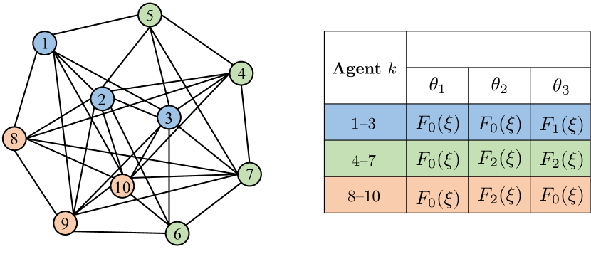
Figure 3: The undirected graph of the network (left) and the local likelihood models of each agent (right).

According to Corollary 2, the uniform Perron eigenvector is an optimal solution to the error exponent maximization problem (41)–(43). To compare the performance of the ASL strategy under different combination policies, we employ 5 left-stochastic combination matrices $A_{1}$–$A_{5}$ and 5 doubly-stochastic combination matrices $A_{6}$–$A_{10}$. These matrices are generated by an iterative method based on the given network topology. For each matrix $A_{i}$, the iterative method starts by generating an initial matrix $A_{0}$ that conforms to the network topology, i.e., $[A_{0}]_{\ell k}>0$ if $\ell\in\mathcal{N}_{k}$ and $[A_{0}]_{\ell k}=0$ otherwise. A left-stochastic combination matrix $A_{i}$ is then constructed by normalizing each column of $A_{0}$. If $A_{i}$ should be doubly-stochastic, then row and column normalization is performed alternatively until convergence. All the combination matrices $A_{1}$–$A_{10}$ are checked to have a positive Perron eigenvector for truth learning.

First, we study the influence of combination policies on the error exponent. To evaluate the steady-state error probability, we consider a stationary environment where the true hypothesis is selected as $\theta_{1}$. We further assume that all agents hold a uniform initial belief. Table I lists the $\theta$-related error exponents $\Phi(\pi,\theta)$ and their approximation $\widehat{\Phi}(\pi,\theta)$ based on (108) (see expression in (163)). It is observed that for all 10 combination matrices, the error exponent in this learning task is determined by the wrong hypothesis $\theta_{3}$. Moreover, the doubly-stochastic matrices deliver a larger error exponent than all left-stochastic ones. Therefore, we can expect that as $\delta\to 0$, the steady-state error probability vanishes to zero with a larger decaying rate when the doubly-stochastic combination policy is employed.

TABLE I: $\Phi(\pi,\theta)$ and $\widehat{\Phi}(\pi,\theta)$ for different combination matrices

Matrix $A$	$\Phi(\pi,\theta_{2})$	$\widehat{\Phi}(\pi,\theta_{2})$	$\Phi(\pi,\theta_{3})$	$\widehat{\Phi}(\pi,\theta_{3})$
$A_{1}$	$0.0578$	$0.0582$	$0.0392$	$0.0394$
$A_{2}$	$0.0464$	$0.0467$	$0.0377$	$0.0379$
$A_{3}$	$0.0536$	$0.0539$	$0.0360$	$0.0362$
$A_{4}$	$0.0567$	$0.0571$	$0.0329$	$0.0331$
$A_{5}$	$0.0543$	$0.0546$	$0.0352$	$0.0354$
$A_{6}$–$A_{10}$	$0.0656$	$0.0660$	$0.0447$	$0.0450$

In Fig. 4, the steady-state error probability averaged across agents, is presented for 10 combination polices and different step-sizes. For each step-size, we select the terminal time as 3000 and run 1000000 Monte Carlo simulations to obtain the average results. It can be observed that the doubly-stochastic combination matrices $A_{6}$–$A_{10}$ lead to a similar steady-state error probability that is smaller than those corresponding to left-stochastic combination matrices $A_{1}$–$A_{5}$. In Fig. 5, we provide the steady-state error probability of 4 agents. Despite the slight differences for different agents, the advantage of doubly-stochastic combination matrices becomes more pronounced as $\delta$ decreases. This is consistent with our conclusion in Corollary 2.

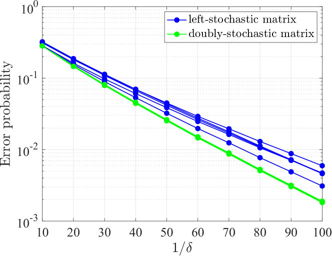
Figure 4: Average steady-state error probability.

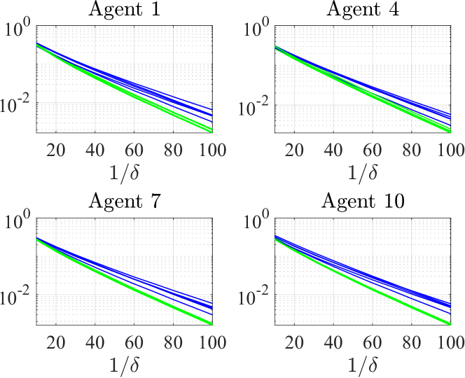
Figure 5: Steady-state error probability of 4 agents. Blue (green) lines denote left (doubly)-stochastic matrices.

Next, we study the effect of combination policies on the adaptation time. Here, we consider a non-stationary environment where the true state changes from $\theta_{1}$ to $\theta_{2}$ at $i=1000$ and from $\theta_{2}$ to $\theta_{3}$ at $i=2000$. Under a small step-size $\delta=0.01$ and a uniform initial belief condition, the transient dynamics of the average instantaneous error probability over $i\in[0,3000]$ is depicted in Fig. 6. An important observation is that, in the non-stationary environment, the adaptation time related to different combination matrices is very close to each other. To derive a quantitative comparison, we calculate the simulated adaptation time when the true state is $\theta_{1}$. Let $p_{{\sf ave},i}$ and $p_{\sf ave}$ denote the average instantaneous error probability at time instant $i$ and the average steady-state error probability, respectively. According to the definition of adaptation time in (105), we record the time instant $i_{0}$ after which the average instantaneous error probability $p_{{\sf ave},i}$ satisfies

$$\log{p_{{\sf ave},i}}\leq(1-\omega)\log{p_{\sf ave}},\quad i\geq i_{0}.$$ (113)

The simulated adaptation time calculated by (113) and its approximation ${\sf T_{adap}}(\omega)$ under different values of $\omega$ is presented in Fig. 7. We also include the approximation $\sf T_{ASL}(\pi,\omega)$ (106) provided in [12]. It is clear that the difference in adaptation time for all considered combination matrices is almost negligible irrespective of $\omega$ in our simulations. Consequently, as observed in Fig. 6, the doubly-stochastic combination policies contribute to a smaller instantaneous error probability during the learning process. This provides a solid foundation for employing a doubly-stochastic combination policy in this learning task. Moreover, we see from Fig. 7 that both approximations ${\sf T_{adap}}(\omega)$ and ${\sf T_{ASL}}(\pi,\omega)$ provide an upper bound on the simulated adaptation time. Compared with ${\sf T_{ASL}}(\pi,\omega)$, which applies to all learning tasks, ${\sf T_{adap}}(\omega)$ discussed for the low SNR regime defines a better bound and illuminates the minor role of combination policies.

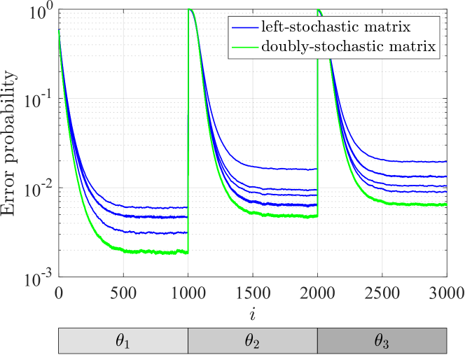
Figure 6: Average instantaneous error probability with $\delta=0.01$. The variation of the true state is depicted in the bottom panel.

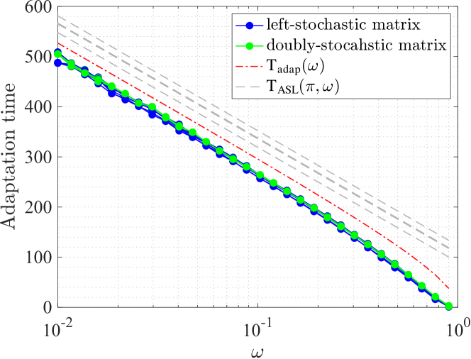
Figure 7: Adaptation time under different combination matrices.

V-B Social learning with noisy shift-in-mean Gaussian model

In this part, we illustrate the learning performance of the ASL strategy (Theorem 1) and the optimal Perron eigenvector $\pi^{\star}$ given by (85) for the noisy shift-in-mean Gaussian model (83). As discussed in Section III-D2, it is not always possible to construct a combination policy with the predefined Perron eigenvector for a given network topology. To avoid this inconvenience, we consider an undirected network (shown in Fig. 3) by adding more edges to the Erdös-Rényi random network considered in Section V-A. Since we have assumed previously that each agent has a self-loop, the construction rule in (104) can be employed to generate a combination policy with any prescribed Perron eigenvector $\pi$ for this undirected network. We also consider a social learning protocol with three hypotheses. The parameters of the considered noisy shift-in-mean Gaussian model are listed in Table II.

TABLE II: Parameters of the noisy shift-in-mean Gaussian model

Agent $k$	${\sf m}_{k}(\theta_{1})$	${\sf m}_{k}(\theta_{2})$	${\sf m}_{k}(\theta_{3})$	$\sigma_{k}^{2}$	$\varepsilon_{k}$	$t_{k}^{\sf nc}(\theta)$
1–3	0	$0.1$	$0.1$	$1$	$1$	$-0.5,-0.5$
4–7	$0.2$	$0$	$0.2$	$2$	$0.1$	$-0.9091,-C$
8–10	$0.3$	$0.3$	$0$	$3$	$0.001$	$-C,-0.9990$

First, we show the learning behavior of the ASL strategy in this task when the true hypothesis is $\theta_{1}$. We consider the uniform averaging rule $a_{\ell k}={1}/{\absolutevalue{\mathcal{N}_{k}}},\forall\ell\in\mathcal{N}_{k}$ where $\absolutevalue{\mathcal{N}_{k}}$ is the cardinality of set $\mathcal{N}_{k}$. Let $\pi^{\sf u}$ be the Perron eigenvector corresponding to the uniform averaging rule, we can derive ${\sf m_{ave}}(\pi^{\sf u},\theta_{2})=0.0052$ and ${\sf m_{ave}}(\pi^{\sf u},\theta_{3})=0.0064$ based on Table II. With $\delta=0.002$ and a uniform initial belief, the time evolution of log-belief ratios $\bm{\lambda}_{k,i}(\theta)$ in one realization is shown in Fig. 8. We can see that for this small step-size, the steady-state log-belief ratios of each agent concentrate around the expectation values ${\sf m_{ave}}(\pi^{\sf u},\theta)$. This shows the consistency of learning with the ASL strategy for the noisy shift-in-mean Gaussian model, as predicted by Theorem 1. Furthermore, we evaluate the estimation performance of the two methods proposed in Section III-D1 on the quantity $t_{k}^{\sf nc}(\theta)$, whose value can be calculated by using (150). The theoretical values of $t_{k}^{\sf nc}(\theta)$ are listed in Table II. We note that under the given parameter configuration, there are no conflicting agents in the network. For one realization, we plot the estimates of $t_{k}^{\sf nc}(\theta)$ for each agent within the first $10000$ observations in Fig. 9. Under the considered noisy shift-in-mean Gaussian model, the estimate of $t_{k}^{\sf nc}(\theta)$ in the indirect estimation method admits a closed-form expression (103). It is clear from Fig. 9 that the indirect estimation method is more efficient than the direct one in our simulations. Since $\bm{x}_{k,i}(\theta)$ is unbounded in Gaussian models, a substantial number of observations will be needed to obtain a good approximation with the direct estimation method.

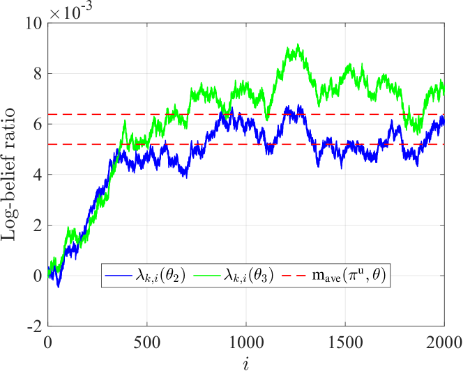
Figure 8: Evolution of log-belief ratios of each agent in one realization.

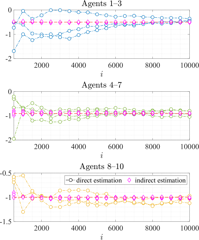
Figure 9: Estimation of $t_{k}^{\sf nc}(\theta)$ after every 500 observations with the direct and indirect estimation methods. The dotted red lines represent the theoretical values of $t_{k}^{\sf nc}(\theta)$. The discretization step-size is 0.01 in the direct estimation method. Curves related to the $\theta$-uninformative agents are removed for clarity.

Next, we consider the effect of combination policies on the error exponent in this noisy learning environment. According to Corollary 3, the maximum error exponent can be achieved by the Perron eigenvector $\pi^{\star}$ in (85). Based on the parameter setting in Table II, we obtain $\pi_{k}^{\star}=0.0615$ for agents 1–3, $\pi_{k}^{\star}=0.1118$ for agents 4–7, and $\pi_{k}^{\star}=0.1228$ for agents 8–10. A left-stochastic combination matrix with Perron eigenvector $\pi^{\star}$ is constructed by following rule (104) and is denoted by $A^{\star}$. For comparison, we introduce another 5 left-stochastic matrices $A_{1}$–$A_{5}$ with different Perron eigenvectors and 5 doubly-stochastic matrices $A_{6}$–$A_{10}$. All 11 combination matrices have a positive Perron eigenvector. With a uniform initial belief, the steady-state error probability of the network and 4 agents for different small step-sizes are presented in Figs. 10 and 11. For each step-size, the terminal time is 3000 and the number of Monte Carlo simulations is $1000000$. It is seen that the combination matrix $A^{\star}$ with Perron eigenvector $\pi^{\star}$ leads to a larger error exponent than that of all other combination policies in comparison. This is consistent with Corollary 3.

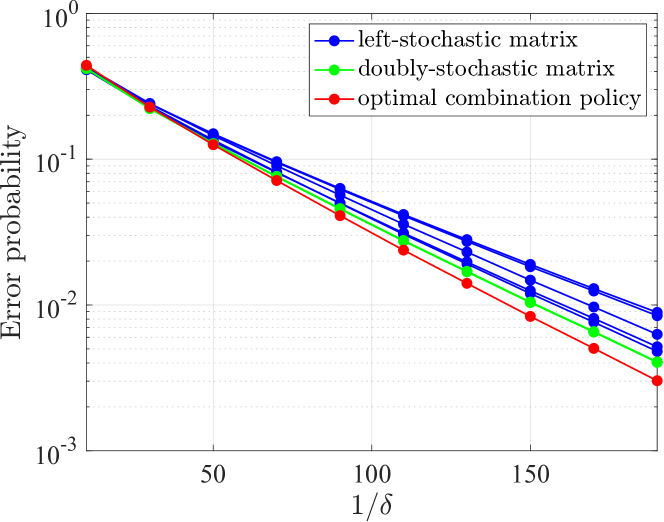
Figure 10: Average steady-state error probability.

Figure 11: Steady-state error probability of each agent. The curve labels are the same as Fig. 10.

Then, we compare the adaptation time of the ASL strategy under different combination policies. From (146), the parabolic approximation (108) holds for the noisy shift-in-mean Gaussian model. We expect that ${\sf T_{adap}}(\omega)$ in Theorem 4 will be a reasonable approximation of the adaptation time in the slow adaptation regime. With $\delta=0.01$ and different $\omega$, we calculate the simulated adaptation time for each combination matrix based on (113) and then compare them with the approximated values $\sf T_{ASL}(\pi,\omega)$ and ${\sf T_{adap}}(\omega)$ given by (106) and (111) respectively. Corresponding results are presented in Fig. 12. It is shown that the effect of combination policies on the adaptation time of the ASL strategy is not significant under the given step-size. The difference between the simulated adaptation time and the theoretical one in (111) comes from the sub-exponential term $\mathcal{O}(\delta)$ in (105). Similar to the observation in Fig. 7, ${\sf T_{adap}}(\omega)$ provides a better characterization of the adaptation time than $\sf T_{ASL}(\pi,\omega)$ for this learning task. Fig. 13 presents the time evolution of the instantaneous error probability in a non-stationary environment, where the true state changes from $\theta_{1}$ to $\theta_{2}$ and from $\theta_{2}$ to $\theta_{3}$ at $i=1000$ and $2000$, respectively. Similar to Fig. 6, the curve related to the optimal combination matrix $A^{\star}$ is lower than all other curves during the whole learning process. Therefore, it is beneficial to employ a combination policy with the best Perron eigenvector for the steady-state learning performance.

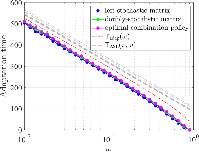
Figure 12: Adaptation time under different combination matrices.

Finally, we examine the case where the optimal combination policy changes with the true state of nature. To simulate this scenario, we assume that the noise level in the private signals is dependent on the underlying state. Specifically, we consider $\varepsilon_{k}=0.1$ (or $0.001$) for agents 1–3, $\varepsilon_{k}=0.001$ (or 1) for agents 4–7, and $\varepsilon_{k}=1$ (or 0.1) for agents 8–10 when the true state is $\theta_{2}$ (or $\theta_{3}$). Based on (85), we compute an optimal Perron eigenvector associated with each hypothesis, which is then used to design the combination policy according to (104). The three resulting optimal combination matrices are denoted by $A_{1}^{\star}$, $A_{2}^{\star}$ and $A_{3}^{\star}$. We study a non-stationary environment similar to Fig. 13, where the true hypothesis changes from $\theta_{1}$ to $\theta_{2}$ at $i=1000$ and then to $\theta_{3}$ at $i=2000$. The evolution of the instantaneous error probabilities associated with $A_{1}^{\star}$–$A_{3}^{\star}$ is presented in Fig. 14. Since the optimization problem (41)–(43) is formulated to maximize the error exponent, the optimal combination policy pertaining the underlying state will deliver a smaller steady-state error probability in the small-$\delta$ regime. On the other hand, we note that our analysis of the adaptation time does not depend on the true hypothesis. Therefore, the conclusion from Theorem 4 is still valid, which implies that the optimal combination policy for the steady-state learning performance does not harm the transient behavior. This is in line with our observations in Fig. 14.

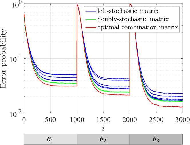
Figure 13: Average instantaneous error probability with $\delta=0.01$. The variation of the true state is depicted in the bottom panel.

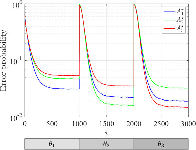
Figure 14: Average instantaneous error probability with $\delta=0.01$. The noise level changes with the variation of the true state depicted in the bottom panel.

VI Concluding Remarks

Combination policies play an important role in the behavior of social learning strategies. In this work, we discussed the effect of combination policies on two key performance metrics: the error exponent (i.e., steady-state learning ability) and the adaptation time (i.e., transient learning behavior) in the slow adaptation regime. For a general signal model, we characterized the performance limits of the error exponent and provided the set of optimal Perron eigenvectors. Moreover, we showed that the difference of the adaptation time under different combination policies is almost negligible if the hypotheses are close to each other. Our findings reveal the important relation between the learning performance of the ASL strategy and the combination policy among agents, which can be useful for the network design of many inference problems.

Several useful extensions and generalizations are possible. One extension refers to the online learning of the optimal combination policy. From Theorems 3a and 3b, we know that the optimal combination policy depends on the critical value $t_{k}^{\sf nc}(\theta)$ that is determined by the LMGF of the log-likelihood ratio variable $\bm{x}_{k,i}(\theta)$. Therefore, full knowledge of the agents’ signal models are needed to construct the optimal combination policy. This raises the question of how to learn the combination policy in an online manner, where the agents infer the underlying truth and estimate $t_{k}^{\sf nc}(\theta)$ with their observations in the same time. This online setting is especially important in the non-stationary environment where the optimal combination policy changes with the true state of nature as shown in Fig. 14.

Another useful generalization concerns the compact space of hypotheses. In this work, we consider a finite number of hypotheses. It will be worthwhile to investigate the cases where the hypothesis is characterized by a continuous parameter. A good reference along these lines for the non-adaptive social learning is [45]. Using the similar variational interpretation of the adaptation step (10), it is straightforward to generalize the ASL algorithm (18) to the continuous space. However, new analytical approaches need to be developed for the performance analysis.

Appendix A Useful properties for the proofs

For the forthcoming proofs, we need some useful properties of the LMGFs $\Lambda_{k}(t;\theta)$ and functions $\phi_{k}^{\sf nc}(t;\theta)$ under the general signal model (3)–(4) as listed in Lemma 1. Similar properties for the accurate signal model (4)–(5) can be found in [12, 33, 34, 22]. The first and second derivatives of a function $f(t)$ will be denoted by $f^{\prime}(t)$ and $f^{\prime\prime}(t)$, respectively.

Lemma 1 (Useful properties).

For each wrong hypothesis $\theta\neq\theta_{1}$, the following properties associated with the LMGF $\Lambda_{k}(t;\theta)$ and function $\phi_{k}^{\sf nc}(t;\theta)$ hold for all agents $k\notin\mathcal{N}^{U}(\theta)$:

1. $\Lambda_{k}(t;\theta)$ is infinitely differentiable in $\mathbb{R}$. Also, it is strictly convex for all $t\in\mathbb{R}$.

2. $\Lambda_{k}(t;\theta)$ has a zero-point at $t=0$. If $d_{k}(\theta)=0$, this zero-point is unique, i.e., $\Lambda_{k}(t;\theta)>0$ for all $t\neq 0$; If $d_{k}(\theta)<0$, $\Lambda_{k}(t;\theta)$ has a positive zero-point $t_{0}$, i.e., $\exists t_{0}>0$ such that $\Lambda_{k}(t_{0};\theta)=0$; If $d_{k}(\theta)>0$, $\Lambda_{k}(t;\theta)$ has a negative zero-point $t_{0}$. In particular, if $f_{k}=L_{k}(\cdot|\theta_{1})$, we have

   $$t_{0}=-1.$$ (114)

3. The function $\frac{\Lambda_{k}(t;\theta)}{t}$ is continuous for all $t\in\mathbb{R}$, with

   $$\underset{t\to 0}{\lim}\frac{\Lambda_{k}(t;\theta)}{t}=\Lambda^{\prime}_{k}(0;\theta)=d_{k}(\theta).$$ (115)

4. $\phi_{k}^{\sf nc}(t;\theta)$ is strictly convex for all $t\in\mathbb{R}$.

Furthermore, the following properties in regard to the LMGF $\Lambda_{\sf ave}(t;\pi,\theta)$ and function $\phi(t;\pi,\theta)$ hold for all feasible Perron eigenvectors $\pi\in\Pi$:

1. $\Lambda_{\sf ave}(t;\pi,\theta)$ and $\phi(t;\pi,\theta)$ are strictly convex for all $t\in\mathbb{R}$.

2. $\Lambda_{\sf ave}(t;\pi,\theta)$ has a negative zero-point.

Proof.

The strict convexity of the LMGF $\Lambda_{k}(t;\theta)$ in property i) is the basis of the subsequent properties ii)–vi). We assume that $\bm{x}_{k,i}(\theta)$ is non-degenerate under the general signal model (3)–(4). Property i) is established by using Cauchy–Schwarz inequality, and the proof can be found in [22, 33, 34].

Since ${\Lambda}_{k}(0;\theta)=0$ and ${\Lambda}_{k}^{\prime}(0;\theta)=d_{k}(\theta)$ for all $k$ and $\theta$, $t=0$ is a zero-point of ${\Lambda}_{k}(t;\theta)$ for all $k$ and $\theta$. Furthermore, the first-order condition of the strictly convex function $\Lambda_{k}(t;\theta)$ gives us

$$\Lambda_{k}(t;\theta)>d_{k}(\theta)t.$$ (116)

Obviously, ${\Lambda}_{k}(t;\theta)>0$ for all $t\neq 0$ when $d_{k}(\theta)=0$. Since the signal and likelihood models share the same support, we have $\lim_{t\to\pm\infty}\Lambda_{k}(t;\theta)=\infty$. If $d_{k}(\theta)\neq 0$, then there exists a unique non-zero zero-point $t_{0}\neq 0$ such that $\Lambda_{k}(t_{0};\theta)=0$. If $d_{k}(\theta)<0$, we have $\Lambda_{k}(t;\theta)\geq d_{k}(\theta)t>0$ for all $t<0$ according to (116). Hence, $\Lambda_{k}(t;\theta)$ has a positive zero-point in this case. Likewise, ${\Lambda}_{k}(t;\theta)$ has a negative zero-point $t_{0}$ for the case of $d_{k}(\theta)>0$. If $f_{k}=L_{k}(\cdot|\theta_{1})$, we obtain $\Lambda_{k}(-1;\theta)=0$, and thus $t_{0}=-1$ is the unique negative zero-point of $\Lambda_{k}(t;\theta)$ as demonstrated in [12].

Property iii) can be proved by applying L’Hôpital’s rule to the continuous function $\Lambda_{k}(t;\theta)$ at $t=0$ [22]. This property further ensures that the function $\phi_{k}^{\sf nc}(t;\theta)$ defined in (54) is well-posed. The second-order derivative of $\phi_{k}^{\sf nc}(t;\theta)$ satisfies

$$\left[{\phi_{k}^{\sf nc}}(t;\theta)\right]^{\prime\prime}\triangleq\;\frac{d}{dt}\frac{\Lambda_{k}(t;\theta)}{t}{=}\;\frac{\Lambda^{\prime}_{k}(t;\theta)t-\Lambda_{k}(t;\theta)}{t^{2}}>0$$ (117)

due to the first-order condition of the strictly convex function $\Lambda_{k}(t;\theta)$. Property iv) follows (117).

Under the independence assumption of local observations over space, the strict convexity of individual LMGF $\Lambda_{k}(t;\theta)$ for all agents $k\notin\mathcal{N}^{U}(\theta)$ (property i)) ensures that $\Lambda_{\sf ave}(t;\pi,\theta)$ is also a strictly convex function for $t\in\mathbb{R}$. The strict convexity of $\phi(t;\pi,\theta)$ can be established in the same way as (117). Property vi) is guaranteed by the consistency condition (34), i.e., ${\sf m_{ave}}(\pi,\theta)>0$ for all $\theta\neq\theta_{1}$. Similar to the proof of property ii), we can prove property vi) using the strict convexity of $\Lambda_{\sf ave}(t;\pi,\theta)$ established in property v). ∎

Appendix B Proof of Theorem 2

First, we show that for each $\theta$-informative agent $k\in\mathcal{N}^{I}(\theta)$, $t_{k}^{\sf nc}(\theta)$ defined in (55) corresponds to a negative zero-point of $\Lambda_{k}(t;\theta)$. According to property iv) in Lemma 1, $\phi_{k}^{\sf nc}(t;\theta)$ is a strictly convex function for $t\in\mathbb{R}$. Therefore, the infimum of $\phi_{k}^{\sf nc}(t;\theta)$ is achieved at its unique stationary point:

$$[\phi_{k}^{\sf nc}(t;\theta)]^{\prime}=\frac{\Lambda_{k}(t;\theta)}{t}=0.$$ (118)

From definition (46), we have $d_{k}(\theta)>0$ for all $k\in\mathcal{N}^{I}(\theta)$. Property iii) shows that the stationary point in (118) corresponds to the negative zero-point of $\Lambda_{k}(t;\theta)$, whose existence and uniqueness are guaranteed by property ii) in Lemma 1. Therefore, $t_{k}^{\sf nc}(\theta)$ is given by

$$t_{k}^{\sf nc}(\theta)=\left\{t\neq 0:{\Lambda}_{k}(t;\theta)=0\right\}<0.$$ (119)

Next, we prove the bound of the error exponent established in Theorem 2. Based on the definition of $t_{k}^{\sf nc}(\theta)$ in (58), we have $t_{k}^{\sf nc}(\theta)\leq 0$ and

$$\Lambda_{k}(t;\theta)\leq 0,\quad\forall t\in[t_{k}^{\sf nc}(\theta),0],$$ (120)

for all agents $k\in\mathcal{N}$. Moreover, $\Phi_{k}^{\sf nc}(\theta)=0$ holds for each $k\notin\mathcal{N}^{I}(\theta)$. This yields

$$\Phi_{\sum}^{\sf nc}(\theta)\triangleq\sum_{k=1}^{N}\Phi_{k}^{\sf nc}(\theta)=\sum_{k\in\mathcal{N}^{I}(\theta)}\Phi_{k}^{\sf nc}(\theta),\quad\forall\theta\neq\theta_{1}.$$ (121)

For any Perron eigenvector $\pi\in\Pi$, we have ${\sf m_{ave}}(\pi,\theta)>0$, $\forall\theta\neq\theta_{1}$ from (43). Due to properties v) and vi) in Lemma 1, the infimum of $\phi(t;\pi,\theta)$ is achieved at its unique stationary point that corresponds to the negative zero-point of $\Lambda_{\sf ave}(t;\pi,\theta)$. Let $t_{\theta}^{\star}(\pi)$ be the critical value corresponding to the $\theta$-related error exponent $\Phi(\pi,\theta)$ in (37), i.e., $\Phi(\pi,\theta)=-\phi(t_{\theta}^{\star}(\pi);\pi,\theta)$. Then, $t_{\theta}^{\star}(\pi)$ is the unique non-zero solution to $\Lambda_{\sf ave}(t;\pi,\theta)=0$:

$$t_{\theta}^{\star}(\pi)=\{t\neq 0:\Lambda_{\sf ave}(t;\pi,\theta)=0\}<0.$$ (122)

Therefore,

$${\Phi}(\pi,\theta) \triangleq-\inf\limits_{t\in\mathbb{R}}{\phi}(t;\pi,\theta)\overset{\eqref{eq: t_theta(pi)}}{=}-\inf_{t<0}\phi(t;\pi,\theta)$$

$$\overset{\textnormal{(a)}}{=}-\inf_{t<0}\sum_{k=1}^{N}{\phi}^{\sf nc}_{k}(\pi_{k}t;\theta)\leq\sum_{k=1}^{N}-\inf_{t<0}{\phi}^{\sf nc}_{k}(\pi_{k}t;\theta)$$

$$\overset{\textnormal{(b)}}{=}\sum_{k\in\mathcal{N}^{I}(\theta)}-\inf_{t<0}{\phi}^{\sf nc}_{k}(t;\theta)=\sum_{k\in\mathcal{N}^{I}(\theta)}{\Phi}^{\sf nc}_{k}(\theta)$$

$$\overset{\eqref{eq: sum of error exponnet of informative agents}}{=}{\Phi}_{\sum}^{\sf nc}(\theta).$$ (123)

where (a) is due to the definitions given in (32), (38), and (54), and (b) comes from (45) and (57). Since the error exponent $\Phi(\pi)$ is determined by the minimum ${\Phi}(\pi,\theta)$ among all wrong hypotheses $\theta\neq\theta_{1}$, we can derive from (123) that

$${\Phi}(\pi)=\min_{\theta\neq\theta_{1}}{\Phi}(\pi,\theta){\leq}\min_{\theta\neq\theta_{1}}{\Phi}_{\sum}^{\sf nc}(\theta).$$ (124)

This implies that each aggregated quantity ${\Phi}_{\sum}^{\sf nc}(\theta)$ is an upper bound of the error exponent $\Phi(\pi)$ for all feasible combination policies. On the other hand, for a given Perron eigenvector $\pi\in\Pi$, we can define the following quantities:

$$k_{\sf m}^{\theta}=\operatorname*{argmax}_{k\in\mathcal{N}}\frac{t_{k}^{\sf nc}(\theta)}{\pi_{k}},\quad t_{\sf m}^{\theta}=\max_{k\in\mathcal{N}}\frac{t_{k}^{\sf nc}(\theta)}{\pi_{k}}.$$ (125)

This yields $\pi_{k_{\sf m}^{\theta}}t_{\sf m}^{\theta}=t_{k_{\sf m}^{\theta}}^{\sf nc}(\theta)$ and $\Phi_{k_{\sf m}^{\theta}}^{\sf nc}(\theta)=-\phi_{k_{\sf m}^{\theta}}^{\sf nc}(\pi_{k_{\sf m}^{\theta}}t_{\sf m}^{\theta};\theta)$. Since $t_{k}^{\sf nc}(\theta)\leq 0,\forall k\in\mathcal{N}$ by definition (58), (125) gives

$$t_{k}^{\sf nc}(\theta)\leq\pi_{k}t_{\sf m}^{\theta}\leq 0,\quad\forall k\in\mathcal{N}.$$ (126)

Then, for each $\theta\neq\theta_{1}$, we have

$${\Phi}(\pi,\theta) \triangleq-\inf\limits_{t\in\mathbb{R}}{\phi}(t;\pi,\theta)\geq-{\phi}(t_{\sf m}^{\theta};\pi,\theta)$$

$${=}-{\phi}^{\sf nc}_{k_{\sf m}^{\theta}}(\pi_{k_{\sf m}^{\theta}}t_{\sf m}^{\theta};\theta)-\sum_{\ell\neq k_{\sf m}^{\theta}}{\phi}^{\sf nc}_{\ell}(\pi_{\ell}t_{\sf m}^{\theta};\theta)$$

$${\geq}{\Phi}^{\sf nc}_{k_{\sf m}^{\theta}}(\theta)\geq\min_{k\in\mathcal{N}}{\Phi}_{k}^{\sf nc}(\theta)$$ (127)

where the inequality (a) comes from (120) and (126):

$${\phi}^{\sf nc}_{\ell}(\pi_{\ell}t_{\sf m}^{\theta};\theta)\triangleq\int_{0}^{\pi_{\ell}t_{\sf m}^{\theta}}\frac{{\Lambda}_{\ell}(\tau;\theta)}{\tau}d\tau\leq 0,\quad\forall\ell\neq k_{\sf m}^{\theta}.$$ (128)

Therefore, the error exponent ${\Phi}(\pi)$ is lower bounded by

$${\Phi}(\pi)=\min_{\theta\neq\theta_{1}}{\Phi}(\pi,\theta){\geq}\min_{\theta\neq\theta_{1}}\min_{k\in\mathcal{N}}{\Phi}_{k}^{\sf nc}(\theta).$$ (129)

The bounds for $\Phi(\pi,\theta)$ and $\Phi(\pi)$ are established using (123), (124), (127) and (129).

Appendix C Proof of Theorems 3a and 3b

C-A Proof of Theorem 3a

In this case, we need to prove that $\Pi^{\dagger}\neq\emptyset$ is a sufficient and necessary condition for achieving the upper bound $\Phi_{\sum}^{\sf nc}(\theta^{\dagger})$, and that the set of optimal Perron eigenvectors is given by $\Pi^{\star}=\Pi^{\dagger}$ when $\Phi^{\star}=\Phi_{\sum}^{\sf nc}(\theta^{\dagger})$. First, we show that $\Pi^{\dagger}\neq\emptyset$ is a sufficient condition for delivering $\Phi^{\star}=\Phi_{\sum}^{\sf nc}(\theta^{\dagger})$. From Theorem 2, ${\Phi}_{\sum}^{\sf nc}(\theta^{\dagger})$ is an upper bound of the error exponent, and thus $\Phi^{\star}\leq\Phi_{\sum}^{\sf nc}(\theta^{\dagger})$. Consider any Perron eigenvector $\pi\in\Pi^{\dagger}$, by definition of $\Pi_{1}$ in (69), we have $\Phi(\pi,\theta^{\dagger})\leq\Phi(\pi,\theta)$, $\forall\theta\neq\theta_{1}$. This means that the error exponent under $\pi$ is determined by hypothesis $\theta^{\dagger}$, i.e., $\Phi(\pi)=\Phi(\pi,\theta^{\dagger})$. According to definition (45), we have $\Lambda_{k}(t;\theta^{\dagger})\equiv 0$ for all agents $k\in\mathcal{N}^{{U}}(\theta^{\dagger})$. This implies that the centrality of the $\theta^{\dagger}$-uninformative agents has no impact on the value of $\Phi(\pi,\theta^{\dagger})$. Recalling the definitions of $t_{k}^{\sf nc}(\theta^{\dagger})$ in (58) and denoting $t_{\sum}^{\sf nc}=\sum_{k=1}^{N}t_{k}^{\sf nc}(\theta^{\dagger})$, we have

$$\Phi(\pi,\theta^{\dagger}) \triangleq-\inf_{t\in\mathbb{R}}{\phi(t;\pi,\theta^{\dagger})}=-\inf_{t\in\mathbb{R}}\sum_{k\notin\mathcal{N}^{U}(\theta^{\dagger})}\phi^{\sf nc}_{k}(\pi_{k}t;\theta^{\dagger})$$

$$\overset{\text{(a)}}{\geq}-\sum_{k\notin\mathcal{N}^{U}(\theta^{\dagger})}\phi^{\sf nc}_{k}(\pi_{k}\frac{t_{\sum}^{\sf nc}}{\alpha};\theta^{\dagger})$$

$${=}-\sum_{k\notin\mathcal{N}^{U}(\theta^{\dagger})}{\phi^{\sf nc}_{k}(t_{k}^{\sf nc}(\theta^{\dagger});\theta^{\dagger})}=-\phi({t_{\sum}^{\sf nc}};\pi^{\dagger},\theta^{\dagger})$$ (130)

where (a) follows by letting $t={t_{\sum}^{\sf nc}}/{\alpha}$. From (67), we obtain $\Phi(\pi^{\dagger},\theta^{\dagger})=-\phi({t_{\sum}^{\sf nc}};\pi^{\dagger},\theta^{\dagger})={\Phi}_{\sum}^{\sf nc}(\theta^{\dagger})$. Then, the optimality of $\pi$ for the error exponent maximization problem (41)–(43) is established by

$$\Phi_{\sum}^{\sf nc}(\theta^{\dagger})\overset{\eqref{eq: bound of error exponent}}{\geq}\Phi^{\star}\geq\Phi(\pi)\overset{\eqref{eq: optimal set-case 1}}{=}\Phi(\pi,\theta^{\dagger})\overset{\eqref{eq: optimality of pi}}{\geq}\Phi_{\sum}^{\sf nc}(\theta^{\dagger}).$$ (131)

This implies that if $\Pi^{\dagger}$ is nonempty, any Perron eigenvector $\pi\in\Pi^{\dagger}$ will deliver an error exponent $\Phi_{\sum}^{\sf nc}(\theta^{\dagger})$. Therefore, the largest error exponent for the optimization problem (41)–(43) is $\Pi^{\star}=\Phi_{\sum}^{\sf nc}(\theta^{\dagger})$.

Next, we show that in this case (i.e., $\Pi^{\dagger}\neq\emptyset$), the set $\Pi^{\star}$ of optimal Perron eigenvectors is given by (71). We noted that in (131), we have shown that any Perron eigenvector $\pi\in\Pi^{\dagger}$ is an optimal solution to the error exponent maximization problem (41)–(43). Therefore, $\Pi^{\dagger}$ is contained in the optimal set $\Pi^{\star}$. That is,

$$\Pi^{\dagger}\subseteq\Pi^{\star}.$$ (132)

It remains to establish the condition in the other direction: $\Pi^{\star}\subseteq\Pi^{\dagger}$. To this end, we analyze the necessary conditions for an optimal Perron eigenvector. Since $\Pi$ is the set of all feasible solutions to the optimization problem (41)–(43), we have $\Pi^{\star}\subseteq\Pi$. By the definition of $\theta^{\dagger}$ in (63), the upper bound $\Phi^{\star}=\Phi_{\sum}^{\sf nc}(\theta^{\dagger})$ can be attained if and only if the error exponent $\Phi(\pi)$ is determined by hypothesis $\theta^{\dagger}$. Therefore, the following inequality

$$\Phi(\pi,\theta^{\dagger})\leq\Phi(\pi,\theta),\quad\forall\theta\neq\theta_{1},$$ (133)

needs to be satisfied for any Perron eigenvector $\pi\in\Pi^{\star}$. Hence, we obtain a necessary condition:

$$\Pi^{\star}\subseteq\Pi_{1}\triangleq\left\{\pi\in\Pi:\Phi(\pi,\theta^{\dagger})\leq\Phi(\pi,\theta),\forall\theta\neq\theta_{1}\right\}.$$ (134)

We next prove that the following proportional relation among all $\theta^{\dagger}$-informative agents, as captured by $\pi^{\dagger}$ in (66):

$$\pi_{k}t_{\ell}^{\sf nc}(\theta^{\dagger})=\pi_{\ell}t_{k}^{\sf nc}(\theta^{\dagger}),\quad\forall k,\ell\in\mathcal{N}^{{I}}(\theta^{\dagger}),$$ (135)

must be satisfied for reaching the upper bound $\Phi_{\sum}^{\sf nc}(\theta^{\dagger})$. For any Perron eigenvector $\pi$ that violates (135), there must exist two $\theta^{\dagger}$-informative agents $m$ and $n$ such that

$$\pi_{m}t_{n}^{\sf nc}(\theta^{\dagger})\neq\pi_{n}t_{m}^{\sf nc}(\theta^{\dagger}).$$ (136)

Then, for any $t\neq 0$, the two equations $\pi_{m}t=t_{m}^{\sf nc}(\theta^{\dagger})$ and $\pi_{n}t=t_{n}^{\sf nc}(\theta^{\dagger})$ cannot be both satisfied. Under Assumption 3, there is at least one $\theta^{\dagger}$-informative agent in the network. Recalling the definition of $t_{\theta}^{\star}(\pi)$ in (122), we obtain $t_{\theta^{\dagger}}^{\star}(\pi)<0$ for any Perron eigenvector $\pi\in\Pi$ in this case. Hence, at least one of the following two conditions is true:

$$\pi_{m}t_{\theta^{\dagger}}^{\star}(\pi)\neq t_{m}^{\sf nc}(\theta^{\dagger})\text{ or }\pi_{n}t_{\theta^{\dagger}}^{\star}(\pi)\neq t_{n}^{\sf nc}(\theta^{\dagger}).$$ (137)

Assume that $\pi_{m}t_{\theta^{\dagger}}^{\star}(\pi)\neq t_{m}^{\sf nc}(\theta^{\dagger})$ is satisfied, then

$$\Phi_{m}^{\sf nc}(\theta^{\dagger}) {=}-\phi_{m}^{\sf nc}(t_{m}^{\sf nc}(\theta^{\dagger});\theta^{\dagger})\overset{\eqref{eq: error exponent individually}}{=}-\inf_{t\in\mathbb{R}}\phi_{m}^{\sf nc}(t;\theta^{\dagger})$$

$${>}-\phi_{m}^{\sf nc}(\pi_{m}t_{\theta^{\dagger}}^{\star}(\pi);\theta^{\dagger}),$$ (138)

where (a) is due to the strict convexity of $\phi_{m}^{\sf nc}(t;\theta)$ provided by property iv) in Lemma 1. Since

$$\Phi(\pi,\theta^{\dagger}) \triangleq-\phi(t_{\theta^{\dagger}}^{\star}(\pi);\pi,\theta^{\dagger})$$

$$=-\sum_{k\neq m}{\phi^{\sf nc}_{k}(\pi_{k}t_{\theta^{\dagger}}^{\star}(\pi);\theta^{\dagger})}-{\phi^{\sf nc}_{m}(\pi_{m}t_{\theta^{\dagger}}^{\star}(\pi);\theta^{\dagger})}$$

$${\leq}\sum_{k\neq m}\Phi_{k}^{\sf nc}(\theta^{\dagger})-\phi_{m}^{\sf nc}(\pi_{m}t_{\theta^{\dagger}}^{\star}(\pi);\theta^{\dagger})$$

$${<}\sum_{k\in\mathcal{N}}\Phi_{k}^{\sf nc}(\theta^{\dagger})\triangleq\Phi_{\sum}^{\sf nc}(\theta^{\dagger}),$$ (139)

we obtain $\Phi(\pi)\leq\Phi(\pi,\theta^{\dagger})<\Phi^{\star}$, which implies that $\pi\notin\Pi^{\star}$. Therefore, the proportional relation (135) among $\theta^{\dagger}$-informative agents is necessary for the optimality of a Perron eigenvector. Let $\Pi_{I}$ be the collection of all Perron eigenvectors that satisfy (135):

$$\Pi_{I}=\left\{\pi:\pi_{k}t_{\ell}^{\sf nc}(\theta^{\dagger})=\pi_{\ell}t_{k}^{\sf nc}(\theta^{\dagger}),\forall k,\ell\in\mathcal{N}^{{I}}(\theta^{\dagger})\right\},$$ (140)

then the following condition holds:

$$\Pi^{\star}\subseteq\Pi_{I}.$$ (141)

In view of the definition of $\pi^{\dagger}$ in (66), $\Pi_{I}$ can be rewritten as

$$\Pi_{I}=\left\{\pi:\pi_{k}=\alpha\pi_{k}^{\dagger},\forall k\in\mathcal{N}^{{I}}(\theta^{\dagger}),\forall\alpha>0\right\}\triangleq\Pi_{2}.$$ (142)

Combining the necessary conditions (134) and (141) yields

$$\Pi^{\star}\subseteq\left\{\Pi_{1}\cap\Pi_{2}\right\}\triangleq\Pi^{\dagger}.$$ (143)

Together with (132), (143) gives $\Pi^{\star}=\Pi^{\dagger}$. This proves that if $\Pi^{\dagger}\neq\emptyset$, the optimization problem (41)–(43) has the solution: $\Phi^{\star}=\Phi_{\sum}^{\sf nc}(\theta^{\dagger})$, and $\Pi^{\star}=\Pi^{\dagger}$. Furthermore, if $\Pi^{\dagger}=\emptyset$, there is no Perron eigenvector $\pi\in\Pi$ that satisfies both necessary conditions (134) and (141). Therefore, the upper bound of the error exponent is not achievable for the given learning task. This completes the proof of Theorem 3a.

C-B Proof of Theorem 3b

In this case, we need to prove that if $\Pi_{\epsilon}^{\dagger}$ is not empty, any Perron eigenvector $\pi\in\Pi_{\epsilon}^{\dagger}$ is $\epsilon$-optimal. In other words, $\Pi_{\epsilon}^{\dagger}\neq\emptyset$ is a sufficient condition for deriving an $\epsilon$-optimal Perron eigenvector. This can be established by repeating our analysis in (130) and (131).

Appendix D Proof of Corollary 3

In this noisy environment, each agent $k$ will receive a noisy private signal at each time instant $i$, which is denoted by $\widehat{\bm{\xi}}_{k,i}$:

$$\widehat{\bm{\xi}}_{k,i}=\bm{\xi}_{k,i}+\bm{n}_{k,i}.$$ (144)

With the shift-in-mean Gaussian model (83), the log-likelihood ratio ${\bm{x}}_{k,i}(\theta)$ of the noisy observation $\widehat{\bm{\xi}}_{k,i}$ is given by

$${\bm{x}}_{k,i}(\theta) \triangleq\log\frac{L_{k}(\widehat{\bm{\xi}}_{k,i}|\theta_{1})}{L_{k}(\widehat{\bm{\xi}}_{k,i}|\theta)}$$ (145)

$$=\frac{{\sf m}_{k}(\theta_{1})-{\sf m}_{k}(\theta)}{\sigma_{k}^{2}}\Big{(}{\widehat{\bm{\xi}}}_{k,i}-\frac{{\sf m}_{k}(\theta)+{\sf m}_{k}(\theta_{1})}{2}\Big{)}$$

$$\overset{\eqref{eq: noisy observations}}{} {=}\frac{{\sf m}_{k}(\theta_{1})-{\sf m}_{k}(\theta)}{\sigma_{k}^{2}}\Big{(}\bm{\xi}_{k,i}+\bm{n}_{k,i}-\frac{{\sf m}_{k}(\theta)+{\sf m}_{k}(\theta_{1})}{2}\Big{)}.$$

The random variable ${\bm{x}}_{k,i}(\theta)$ follows a Gaussian distribution:

$${\bm{x}}_{k,i}(\theta)\sim{\sf N}(a_{k}(\theta),b_{k}^{2}(\theta))$$ (146)

with

$$\begin{cases}a_{k}(\theta)=\frac{({\sf m}_{k}(\theta_{1})-{\sf m}_{k}(\theta))^{2}}{2\sigma^{2}_{k}},\\ b_{k}^{2}(\theta)=\frac{({\sf m}_{k}(\theta_{1})-{\sf m}_{k}(\theta))^{2}}{\sigma_{k}^{2}}\left(1+\varepsilon_{k}\right).\end{cases}$$ (147)

It is straightforward to see that $d_{k}(\theta)=a_{k}(\theta)\geq 0$. Since the LMGF of a Gaussian random variable $\bm{y}\sim{\sf N}(a,b)$ is given by $at+bt^{2}/2$, (146) yields

$${\Lambda}_{k}(t;\theta)=a_{k}(\theta)t+\frac{b_{k}^{2}(\theta)}{2}t^{2}.$$ (148)

From (147), we know that $\Lambda_{k}(t;\theta)\equiv 0$ if $a_{k}(\theta)=0$. This implies $\mathcal{N}^{{C}}(\theta)=\emptyset$ according to definition (47). Furthermore, the consistency condition (34) is not impacted by the Gaussian noises. That is,

$${\sf m_{ave}}(\pi,\theta)>0,\quad\forall\theta\neq\theta_{1},$$ (149)

for all Perron eigenvector $\pi$. For any wrong hypothesis $\theta\neq\theta_{1}$, the quantities $t_{k}^{\sf nc}(\theta)$ and $\Phi_{k}^{\sf nc}(\theta)$ of each $\theta$-informative agent $k$ now admit an explicit expression:

$$t_{k}^{\sf nc}(\theta) =-\frac{2a_{k}(\theta)}{b_{k}^{2}(\theta)}=-\frac{1}{1+\varepsilon_{k}},$$ (150)

$${\Phi}_{k}^{\sf nc}(\theta) =\frac{a_{k}(\theta)^{2}}{b_{k}^{2}(\theta)}=\frac{\left({\sf m}_{k}(\theta_{1})-{\sf m}_{k}(\theta)\right)^{2}}{4\sigma_{k}^{2}(1+\varepsilon_{k})}.$$ (151)

It can be observed from (150) that $t_{k}^{\sf nc}(\theta)$ is determined only by the noise level $\varepsilon_{k}$, and thus it is identical for all hypothesis $\theta\neq\theta_{1}$. Moreover, according to (58), the critical value $t_{k}^{\sf nc}(\theta)$ associated with a $\theta$-uninformative agent $k$ can be set to any value. Assume that $t_{k}^{\sf nc}(\theta)=-1/(1+\varepsilon_{k})$ (i.e., following the same expression as (150)) for each $\theta$-uninformative agent $k\in\mathcal{N}^{U}(\theta)$, then from (66), we obtain

$$\pi_{k}^{\dagger} =\frac{\left(1+\varepsilon_{k}\right)^{-1}}{\sum_{\ell=1}^{N}\left(1+\varepsilon_{\ell}\right)^{-1}},$$ (152)

$${\Phi}^{\sf nc}(\theta^{\dagger}) =\min_{\theta\neq\theta_{1}}\sum_{k=1}^{N}\frac{\left({\sf m}_{k}(\theta_{1})-{\sf m}_{k}(\theta)\right)^{2}}{4\sigma_{k}^{2}(1+\varepsilon_{k})}.$$ (153)

It is noted that based on above definitions, the critical value $t_{k}^{\sf nc}(\theta)$ does not depend on the associated hypothesis $\theta$. This means that the Perron eigenvector $\pi^{\dagger}$ is feasible to reach the upper bound $\Phi_{\sum}^{\sf nc}(\theta)$ corresponding to any wrong hypothesis $\theta$. That is, by repeating the same arguments used in (67), we have

$$\Phi(\pi^{\dagger},\theta)=\Phi_{\sum}^{\sf nc}(\theta),\quad\forall\theta\neq\theta_{1}.$$ (154)

By definition (63), we obtain $\Phi(\pi^{\dagger},\theta^{\dagger})<\Phi(\pi^{\dagger},\theta)$, $\forall\theta\neq\theta_{1}$, and thus $\pi^{\dagger}\in\Pi_{1}$. Since $\pi^{\dagger}$ is always an element of set $\Pi_{2}$, we have $\Pi^{\dagger}\neq\emptyset$ and $\pi^{\dagger}\in\Pi^{\dagger}$. Therefore, $\pi^{\star}=\pi^{\dagger}$ is an optimal solution to the the error exponent maximization problem (41)–(43), with $\Phi^{\star}=\Phi_{\sum}^{\sf nc}(\theta^{\dagger})$ given by (153).

Appendix E Proof of Theorem 4

Under the uniform initial belief condition (i.e., $\bm{\lambda}_{k,0}(\theta)=0$ for all $k\in\mathcal{N}$ and $\theta\in\Theta$), we can obtain from (19) that

$$\bm{\lambda}_{k,i}(\theta) =\delta\sum_{m=0}^{i-1}\sum_{\ell=1}^{N}(1-\delta)^{m}[A^{m+1}]_{\ell k}\bm{x}_{\ell,i-m}(\theta)$$

$$=\widehat{\bm{\lambda}}_{k,i}(\theta)\overset{\text{d}}{=}\widetilde{\bm{\lambda}}_{k,i}(\theta)$$ (155)

where $\widehat{\bm{\lambda}}_{k,i}(\theta)$ and $\widetilde{\bm{\lambda}}_{k,i}(\theta)$ are respectively defined in (20) and (21), and the equality in distribution is due to (22). According to (16), the instantaneous error probability of agent $k$ at time instant $i$ associated with $\theta\neq\theta_{1}$ is given by

$$\mathbb{P}\left[\bm{\lambda}_{k,i}(\theta)\leq 0\right] =\mathbb{P}\left[\widetilde{\bm{\lambda}}_{k,i}(\theta)\leq 0\right]$$

$${=}\;\mathbb{P}\left[\frac{t_{\theta}^{\star}(\pi)}{\delta}\widetilde{\bm{\lambda}}_{k,i}(\theta)\geq 0\right]$$

$${\leq}\mathbb{E}\left[\exp(\frac{t_{\theta}^{\star}(\pi)}{\delta}\widetilde{\bm{\lambda}}_{k,i}(\theta))\right],$$ (156)

where (a) is due to $t_{\theta}^{\star}(\pi)<0$ from (122) and (b) follows by applying Markov’s inequality. Denoting the LMGF of $\widetilde{\bm{\lambda}}_{k,i}(\theta)$ as

$$\Lambda_{k,i}(t;\theta)\triangleq\log\mathbb{E}\left[e^{t\widetilde{\bm{\lambda}}_{k,i}(\theta)}\right],$$ (157)

the independence assumption of the local observations over time and space gives

$$\Lambda_{k,i}(t;\theta)=\sum_{m=0}^{i-1}\sum_{\ell=1}^{N}\Lambda_{\ell}\left(\delta(1-\delta)^{m}[A^{m+1}]_{\ell k}t;\theta\right).$$ (158)

Let $b_{i}=[A^{i+1}]_{\ell k}$ and using Eqs. (85) and (86) from [23], we have

$$\Lambda_{k,i}(t;\theta) {=}\sum_{\ell=1}^{N}\sum_{m=0}^{i-1}\Lambda_{\ell}\left(\delta(1-\delta)^{m}[A^{m+1}]_{\ell k}t;\theta\right)$$

$$=\sum_{\ell=1}^{N}\frac{1}{\delta}\left[\int_{\delta(1-\delta)^{i}t}^{\delta t}\frac{\Lambda_{\ell}(\pi_{\ell}\tau;\theta)}{\tau}d\tau+\mathcal{O}(\delta)\right]$$

$$=\frac{1}{\delta}\left[\int_{\delta(1-\delta)^{i}t}^{\delta t}\frac{\Lambda_{\sf ave}(\tau;\pi,\theta)}{\tau}d\tau+\mathcal{O}(\delta)\right].$$ (159)

Let $t=t_{\theta}^{\star}(\pi)/\delta$, we obtain the following expression:

$$\Lambda_{k,i}\left(\frac{t_{\theta}^{\star}(\pi)}{\delta};\theta\right)=\frac{1}{\delta}\Bigg{[}\int_{(1-\delta)^{i}t_{\theta}^{\star}(\pi)}^{t^{\star}_{\theta}(\pi)}\frac{\Lambda_{\sf ave}(\tau;\pi,\theta)}{\tau}d\tau+\mathcal{O}(\delta)\Bigg{]}.$$ (160)

Applying the parabolic approximation (108) in the low SNR regime, we have

$$\frac{\Lambda_{\sf ave}(t;\pi,\theta)}{t}\approx\kappa_{1}(\pi,\theta)+\frac{\kappa_{2}(\pi,\theta)}{2}t$$ (161)

for $t\in[t^{\star}_{\theta}(\pi),0]$. Therefore, we can approximate $t^{\star}_{\theta}(\pi)$ and $\Phi(\pi,\theta)$ as

$$\widehat{t^{\star}_{\theta}}(\pi) \triangleq-\frac{2\kappa_{1}(\pi,\theta)}{\kappa_{2}(\pi,\theta)}=-\frac{2{\sf m_{ave}}(\pi,\theta)}{{\sf c_{ave}(\pi,\theta)}},$$ (162)

$$\widehat{\Phi}(\pi,\theta) \triangleq-\frac{\kappa_{1}(\pi,\theta)^{2}}{\kappa_{2}(\pi,\theta)}=-\frac{{\sf m}_{\sf ave}(\pi,\theta)^{2}}{{\sf c_{ave}(\pi,\theta)}}.$$ (163)

With the expressions of $\widehat{t^{\star}_{\theta}}(\pi)$ and $\widehat{\Phi}(\pi,\theta)$, an approximation for (160) is obtained:

$$\quad\;\Lambda_{k,i}\left(\frac{t_{\theta}^{\star}(\pi)}{\delta};\theta\right)$$

$$\approx\frac{1}{\delta}\left[\int_{(1-\delta)^{i}\widehat{t_{\theta}^{\star}}(\pi)}^{\widehat{t^{\star}_{\theta}}(\pi)}\left\{\kappa_{1}(\pi,\theta)+\frac{\kappa_{2}(\pi,\theta)}{2}\tau\right\}d\tau+\mathcal{O}(\delta)\right]$$

$$=-\frac{1}{\delta}\left\{\left[1-(1-\delta)^{i}\right]^{2}\widehat{\Phi}(\pi,\theta)+\mathcal{O}(\delta)\right\}$$

$$\approx-\frac{1}{\delta}\Bigg{\{}\underbrace{\left[1-(1-\delta)^{i}\right]^{2}}_{\text{denoted as }\eta(\delta,i)}\Phi(\pi,\theta)+\mathcal{O}(\delta)\Bigg{\}}.$$ (164)

Combining (156) and (164), the instantaneous error probability of agent $k$ at time instant $i$ associated with $\theta\neq\theta_{1}$ is upper bounded by

$$\mathbb{P}\left[\bm{\lambda}_{k,i}(\theta)\leq 0\right] \leq\exp\left[\Lambda_{k,i}\left(\frac{t_{\theta}^{\star}(\pi)}{\delta};\theta\right)\right]$$

$$\approx\exp\left\{-\frac{1}{\delta}\big{[}\eta(\delta,i)\Phi(\pi,\theta)+\mathcal{O}(\delta)\big{]}\right\}.$$ (165)

For a given small $\omega>0$ in (105), we let $\eta(\delta,i)\geq 1-\omega$ and then obtain

$$i\geq\dfrac{\log(1-\sqrt{1-\omega})}{\log(1-\delta)}.$$ (166)

The right-hand side of (166) is exactly the definition of ${\sf T_{adap}}(\omega)$ given in Theorem 4. Using Boole’s inequality, the instantaneous error probability $p_{k,i}$ satisfies

$$p_{k,i} =\mathbb{P}\Bigg{[}\bigcup_{\theta\neq\theta_{1}}{\bm{\lambda}}_{k,i}(\theta)\leq 0\Bigg{]}$$

$$\leq\sum_{\theta\neq\theta_{1}}\mathbb{P}\left[{\bm{\lambda}}_{k,i}(\theta)\leq 0\right]$$

$${\approx}\sum_{\theta\neq\theta_{1}}\exp\left\{-\frac{1}{\delta}\left[\eta(\delta,i)\Phi(\pi,\theta)+\mathcal{O}(\delta)\right]\right\}$$

$${\leq}\sum_{\theta\neq\theta_{1}}{e^{-\frac{1}{\delta}\big{[}(1-\omega)\Phi(\pi,\theta)+\mathcal{O}(\delta)\big{]}}}$$

$$\doteq e^{-\frac{1}{\delta}\big{[}(1-\omega)\Phi(\pi)+\mathcal{O}(\delta)\big{]}}$$ (167)

for $i\geq{\sf T_{adap}}(\omega)$, which shows that the condition in (105) is satisfied. Hence, ${\sf T_{adap}}(\omega)$ provides a reasonable estimate for the adaptation time of the ASL strategy in the low SNR regime.

References

• [1] P. Hu, V. Bordignon, S. Vlaski, and A. H. Sayed, “Optimal combination policies for adaptive social learning,” in Proc. IEEE ICASSP, Singapore, May 2022, pp. 1–5.
• [2] P. Molavi, A. Tahbaz-Salehi, and A. Jadbabaie, “A theory of non-Bayesian social learning,” Econometrica, vol. 86, no. 2, pp. 445–490, 2018.
• [3] A. Jadbabaie, P. Molavi, A. Sandroni, and A. Tahbaz-Salehi, “Non-Bayesian social learning,” Games and Economic Behavior, vol. 76, no. 1, pp. 210–225, 2012.
• [4] X. Zhao and A. H. Sayed, “Learning over social networks via diffusion adaptation,” in Proc. Asilomar Conference on Signals, Systems and Computers, Pacific Grove, USA, 2012, pp. 709–713.
• [5] H. Salami, B. Ying, and A. H. Sayed, “Social learning over weakly connected graphs,” IEEE Transactions on Signal and Information Processing over Networks, vol. 3, no. 2, pp. 222–238, 2017.
• [6] A. Lalitha, T. Javidi, and A. D. Sarwate, “Social learning and distributed hypothesis testing,” IEEE Transactions on Information Theory, vol. 64, no. 9, pp. 6161–6179, 2018.
• [7] A. Nedic, A. Olshevsky, and C. A. Uribe, “Fast convergence rates for distributed non-Bayesian learning,” IEEE Transactions on Automatic Control, vol. 62, no. 11, pp. 5538–5553, 2017.
• [8] J. Z. Hare, C. A. Uribe, L. Kaplan, and A. Jadbabaie, “A general framework for distributed inference with uncertain models,” IEEE Transactions on Signal and Information Processing over Networks, vol. 7, pp. 392–405, 2021.
• [9] V. Matta, V. Bordignon, A. Santos, and A. H. Sayed, “Interplay between topology and social learning over weak graphs,” IEEE Open Journal of Signal Processing, vol. 1, pp. 99–119, 2020.
• [10] C.-X. Shi and G.-H. Yang, “Distributed learning over networks: Effect of using historical observations,” IEEE Transactions on Automatic Control, vol. 65, no. 12, pp. 5503–5509, 2020.
• [11] A. Mitra, J. A. Richards, and S. Sundaram, “A new approach to distributed hypothesis testing and non-Bayesian learning: Improved learning rate and byzantine-resilience,” IEEE Transactions on Automatic Control, vol. 66, no. 9, pp. 4084–4100, 2021.
• [12] V. Bordignon, V. Matta, and A. H. Sayed, “Adaptive social learning,” IEEE Transactions on Information Theory, vol. 67, no. 9, pp. 6053–6081, 2021.
• [13] A. Jadbabaie, P. Molavi, and A. Tahbaz-Salehi, “Information heterogeneity and the speed of learning in social networks,” Columbia Business School Research Paper, no. 13-28, 2013.
• [14] S. Shahrampour, A. Rakhlin, and A. Jadbabaie, “Distributed detection: Finite-time analysis and impact of network topology,” IEEE Transactions on Automatic Control, vol. 61, no. 11, pp. 3256–3268, 2016.
• [15] R. Viswanathan and P. Varshney, “Distributed detection with multiple sensors: Part I–Fundamentals,” Proceedings of the IEEE, vol. 85, no. 1, pp. 54–63, 1997.
• [16] R. Blum, S. Kassam, and H. Poor, “Distributed detection with multiple sensors: Part II–Advanced topics,” Proceedings of the IEEE, vol. 85, no. 1, pp. 64–79, 1997.
• [17] J.-F. Chamberland and V. Veeravalli, “Decentralized detection in sensor networks,” IEEE Transactions on Signal Processing, vol. 51, no. 2, pp. 407–416, 2003.
• [18] V. Matta and A. H. Sayed, “Estimation and detection over adaptive networks,” in Cooperative and Graph Signal Processing, P. M. Djurić and C. Richard, Eds.   Amsterdam, The Netherlands: Elsevier, 2018, pp. 69–106.
• [19] D. Bajovic, D. Jakovetic, J. Xavier, B. Sinopoli, and J. M. F. Moura, “Distributed detection via Gaussian running consensus: Large deviations asymptotic analysis,” IEEE Transactions on Signal Processing, vol. 59, no. 9, pp. 4381–4396, 2011.
• [20] D. Bajovic, D. Jakovetic, J. M. F. Moura, J. Xavier, and B. Sinopoli, “Large deviations performance of consensus+innovations distributed detection with non-Gaussian observations,” IEEE Transactions on Signal Processing, vol. 60, no. 11, pp. 5987–6002, 2012.
• [21] D. Bajovic, J. M. F. Moura, J. Xavier, and B. Sinopoli, “Distributed inference over directed networks: Performance limits and optimal design,” IEEE Transactions on Signal Processing, vol. 64, no. 13, pp. 3308–3323, 2016.
• [22] V. Matta, P. Braca, S. Marano, and A. H. Sayed, “Diffusion-based adaptive distributed detection: Steady-state performance in the slow adaptation regime,” IEEE Transactions on Information Theory, vol. 62, no. 8, pp. 4710–4732, 2016.
• [23] ——, “Distributed detection over adaptive networks: Refined asymptotics and the role of connectivity,” IEEE Transactions on Signal and Information Processing over Networks, vol. 2, no. 4, pp. 442–460, 2016.
• [24] S. Marano and A. H. Sayed, “Decision learning and adaptation over multi-task networks,” IEEE Transactions on Signal Processing, vol. 69, pp. 2873–2887, 2021.
• [25] A. H. Sayed, “Adaptation, learning, and optimization over networks,” Foundations and Trends in Machine Learning, vol. 7, no. 4-5, pp. 311–801, 2014.
• [26] M. Newman, Networks.   Oxford University Press, 2018.
• [27] T. G. Lewis, Network Science: Theory and Applications.   John Wiley & Sons, 2011.
• [28] A. H. Sayed, “Adaptive networks,” Proceedings of the IEEE, vol. 102, no. 4, pp. 460–497, 2014.
• [29] T. M. Cover and J. A. Thomas, Elements of Information Theory.   Hoboken, NJ, USA: Wiley, 1991.
• [30] G. Koliander, Y. El-Laham, P. M. Djurić, and F. Hlawatsch, “Fusion of probability density functions,” Proceedings of the IEEE, vol. 110, no. 4, pp. 404–453, 2022.
• [31] V. Shumovskaia, M. Kayaalp, M. Cemri, and A. H. Sayed, “Discovering influencers in opinion formation over social graphs,” IEEE Open Journal of Signal Processing, pp. 1–20, 2023.
• [32] V. Bordignon, S. Vlaski, V. Matta, and A. H. Sayed, “Learning from heterogeneous data based on social interactions over graphs,” IEEE Transactions on Information Theory, vol. 69, no. 5, pp. 3347–3371, 2023.
• [33] A. Dembo and O. Zeitouni, Large Deviations Techniques and Applications.   Springer, 1998.
• [34] F. Den Hollander, Large Deviations.   American Mathematical Society, 2008.
• [35] C. M. Rohwer, F. Angeletti, and H. Touchette, “Convergence of large-deviation estimators,” Physical Review E, vol. 92, no. 5, p. 052104, 2015.
• [36] F. Nielsen, “An information-geometric characterization of Chernoff information,” IEEE Signal Processing Letters, vol. 20, no. 3, pp. 269–272, 2013.
• [37] A. H. Sayed, Inference and Learning from Data.   Cambridge University Press, 2022.
• [38] M. Chu and G. Golub, Inverse Eigenvalue Problems: Theory, Algorithms, and Applications.   Oxford University Press, June 2005.
• [39] C. F. Borges, R. Frezza, and W. B. Gragg, “Some inverse eigenproblems for Jacobi and arrow matrices,” Numerical Linear Algebra with Applications, vol. 2, no. 3, pp. 195–203, 1995.
• [40] M. T. Chu and M. A. Erbrecht, “Symmetric Toeplitz matrices with two prescribed eigenpairs,” SIAM Journal on Matrix Analysis and Applications, vol. 15, no. 2, pp. 623–635, 1994.
• [41] S.-L. J. Hu and H. Li, “A systematic linear space approach to solving partially described inverse eigenvalue problems,” Inverse Problems, vol. 24, no. 3, p. 035014, 2008.
• [42] S. Vlaski, L. Vandenberghe, and A. H. Sayed, “Regularized diffusion adaptation via conjugate smoothing,” IEEE Transactions on Automatic Control, vol. 67, no. 5, pp. 2343–2358, 2022.
• [43] P. Braca, S. Marano, V. Matta, and P. Willett, “Asymptotic optimality of running consensus in testing binary hypotheses,” IEEE Transactions on Signal Processing, vol. 58, no. 2, pp. 814–825, 2009.
• [44] S. A. Kassam, Signal Detection in Non-Gaussian Noise.   Springer, 1987.
• [45] C. A. Uribe, A. Olshevsky, and A. Nedić, “Nonasymptotic concentration rates in cooperative learning—Part II: Inference on compact hypothesis sets,” IEEE Transactions on Control of Network Systems, vol. 9, no. 3, pp. 1141–1153, 2022.