KEK-TH-2400

Motoi Endo^(a,b,c), Koichi Hamaguchi^(c,d), Sho Iwamoto^(e), Shin-ichi Kawada^(f), Teppei Kitahara^(g,h), Takeo Moroi^(c,d) and Taikan Suehara⁽ⁱ⁾

^(a) KEK Theory Center, IPNS, KEK, Tsukuba, Ibaraki 305–0801, Japan
^(b) The Graduate University of Advanced Studies (Sokendai), Tsukuba, Ibaraki 305–0801, Japan
^(c) Kavli IPMU (WPI), UTIAS, The University of Tokyo, Kashiwa, Chiba 277–8583, Japan
^(d) Department of Physics, The University of Tokyo, Bunkyo-ku, Tokyo 113–0033, Japan
^(e) ELTE E”otv”os Lor’and University, P’azm’any P’eter s’et’any 1/A, Budapest H-1117, Hungary
^(f) IPNS, KEK, Tsukuba, Ibaraki 305–0801, Japan
^(g) Institute for Advanced Research, Nagoya University, Nagoya 464–8601, Japan
^(h) Kobayashi-Maskawa Institute for the Origin of Particles and the Universe, Nagoya University, Nagoya 464–8602, Japan
⁽ⁱ⁾ Department of Physics, Kyushu University, Fukuoka 819–0395, Japan

1 Introduction

The Fermilab experiment of measuring the muon anomalous magnetic moment (muon $g-2$) confirmed the long-standing discrepancy between its measured value at the Brookhaven experiment [1, 2, 3, 4] and the Standard Model (SM) prediction [5],

$${a_{\mu}^{\mathrm{\text{BNL}+\text{FNAL}}}} =\left(11\,659\,206.1\pm 4.1\right)\times 10^{-10}\,,$$ (1)

$${a_{\mu}^{\mathrm{\text{SM}}}} =\left(11\,659\,181.0\pm 4.3\right)\times 10^{-10}\,,$$ (2)

which amounts to a discrepancy at the $4.2\sigma$ level:

$$\Delta a_{\mu}\equiv{a_{\mu}^{\mathrm{\text{BNL}+\text{FNAL}}}}-{a_{\mu}^{\mathrm{\text{SM}}}}=\left(25.1\pm 5.9\right)\times 10^{-10}\,,$$ (3)

where $a_{\mu}\equiv(g_{\mu}-2)/2$ with $g_{\mu}$ being the muon magnetic moment. This discrepancy may be a hint for physics beyond the SM. Noting that $\Delta a_{\mu}$ is as large as the SM electroweak contribution to ${a_{\mu}}$, new particles with a mass at the electroweak scale may be the source of this discrepancy.

Low-energy supersymmetry (SUSY) is one of such solutions [7, 8, 9]. It predicts new particles (SUSY particles) that interact with muons and photons, yielding extra contribution to $a_{\mu}$, which we call ${a_{\mu}^{\mathrm{SUSY}}}$. If their masses are at the sub-TeV scale, ${a_{\mu}^{\mathrm{SUSY}}}$ can be sizable enough to solve the discrepancy. This feature does not harm other benefits of SUSY. In particular, with the thermal freeze-out mechanism, the lightest SUSY particle (LSP) can account for dark matter, with a relic density consistent with the observed value. For example, Ref. [6] pointed out that there exist parameter spaces of the minimal supersymmetric Standard Model (MSSM) in which the muon $g-2$ anomaly is well explained, the LSP becomes the dark matter candidate with the observed relic density, and the latest constraints from collider experiments and dark matter direct detections are avoided.

As the SUSY solution to the muon $g-2$ anomaly requires some SUSY particles to be relatively light, those particles are important targets of future collider experiments. More interestingly, by determining the properties of the SUSY particles, the SUSY contribution ${a_{\mu}^{\mathrm{SUSY}}}$ can be reconstructed to confirm that the anomaly truly originates in SUSY particles [10]. For this purpose, masses and coupling constants of the SUSY particles should be precisely measured.

The International Linear Collider (ILC) is an ideal facility to perform such measurements. Although the SUSY contribution ${a_{\mu}^{\mathrm{SUSY}}}$ comes from various diagrams, we focus on the so-called Bino-smuon diagram (Fig. 1); we denote its contribution by $a_{\mu}^{(\tilde{B})}$. In the parameter space with a large Higgsino mass parameter $\mu\gg 1\,\mathrm{TeV}$, it tends to dominate the SUSY contribution ${a_{\mu}^{\mathrm{SUSY}}}$. The four benchmark points in Ref. [6], BLR1–4, are such examples; Binos $\tilde{B}$ and smuons $\tilde{\mu}_{\mathrm{L,R}}$ are as light as 100–$200\,\mathrm{GeV}$ and $\mu\gg 1\,\mathrm{TeV}$, which realizes ${a_{\mu}^{\mathrm{SUSY}}}\simeq a_{\mu}^{(\tilde{B})}\simeq\Delta a_{\mu}$. In addition, staus $\tilde{\tau}_{\mathrm{1,2}}$ and tau-sneutrinos $\tilde{\nu}_{\tau}$ have masses smaller than $250\,\mathrm{GeV}$ and coannihilation yields the correct dark matter relic abundance. These particles are thus within the reach of the ILC with center-of-mass energy $\sqrt{s}=500\,\mathrm{GeV}$, and we can reconstruct $a_{\mu}^{(\tilde{B})}$ by measuring their properties.

For the reconstruction of $a_{\mu}^{(\tilde{B})}$, it is necessary to know (i) masses of smuons, (ii) Bino (i.e., the lightest neutralino) mass, (iii) lepton-slepton-Bino couplings, and (iv) left-right mixing of the smuons $m_{\tilde{\mu}\mathrm{LR}}^{2}$ (cf. Eq. (5)) as depicted in Fig. 1. Among them, (i)–(iii) can be precisely determined by using the smuon and selectron production processes, as summarized in Ref. [10]. On the contrary, the determination of the left-right mixing of the smuons is highly non-trivial. Information about the smuon left-right mixing is difficult to obtain from the smuon production processes at the ILC because $m_{\tilde{\mu}\mathrm{LR}}^{2}$ is proportional to the muon mass and is tiny relative to the squared smuon masses.

In Ref. [10], it has been proposed to rely on a SUSY relation to determine $m_{\tilde{\mu}\mathrm{LR}}^{2}$. In the parameter region of our interest, i.e., if the Higgsino mass $\mu$ is much larger than the slepton trilinear couplings (the $A_{l}$ parameters), the left-right mixings of the sleptons are approximated by $m_{\tilde{l}\mathrm{LR}}^{2}\simeq-m_{l}\mu\tan\beta$ with $l=e$, $\mu$, and $\tau$ and $\tan\beta$ being the ratio of the vacuum expectation values of up- and down-type Higgs bosons. Then, $m_{\tilde{\mu}\mathrm{LR}}^{2}$ can be related to $m_{\tilde{\tau}\mathrm{LR}}^{2}$ as

$$m_{\tilde{\mu}{LR}}^{2}=\frac{m_{\mu}}{m_{\tau}}m_{\tilde{\tau}{LR}}^{2}\,.$$ (4)

The left-right mixing of the staus is an order of magnitude larger than that of the smuons and hence is easier to measure at the ILC. This provides a strong motivation to study stau properties at the ILC in connection with the muon $g-2$ anomaly. The ILC’s potential to determine the stau properties in the parameter region motivated by the muon $g-2$ anomaly, however, is not yet well understood.

Figure 1: The Bino-smuon loop diagram contributing to ${a_{\mu}^{\mathrm{SUSY}}}$.

Motivated by the possibility to reconstruct the SUSY contribution to the muon $g-2$, we investigate the prospect of measuring stau properties at the ILC. We pay particular attention to the parameter region suggested by the muon $g-2$ anomaly. We perform a detailed Monte Carlo (MC) analysis to see the accuracy of the ILC measurements of the stau mass and mixing parameters. We also qualitatively discuss the implication of the stau study for the reconstruction of ${a_{\mu}^{\mathrm{SUSY}}}$.

This work is organized as follows. In Section 2, we explain our basic strategy to study the stau properties at the ILC. In Section 3, we show the results of our MC analysis. Implication of the stau study to the muon $g-2$ anomaly is discussed in Section 4. The results are summarized in Section 5.

2 Stau Study at the ILC: Basic Strategy

Let us begin with our strategy for the determination of the stau property at the ILC, in particular the stau left-right parameter $m_{\tilde{\tau}\mathrm{LR}}^{2}$, which is used in the reconstruction of ${a_{\mu}^{\mathrm{(\tilde{B})}}}$ in Sec. 4.

The stau mass eigenstates are denoted as $\tilde{\tau}_{1}$ and $\tilde{\tau}_{2}$ (with their masses $m_{\tilde{\tau}_{1}}$ and $m_{\tilde{\tau}_{2}}$), while the gauge eigenstates as $\tilde{\tau}_{L}$ and $\tilde{\tau}_{R}$ (where $\tilde{\tau}_{L}$ is embedded in $SU(2)_{L}$ doublet while $\tilde{\tau}_{R}$ is $SU(2)_{L}$ singlet). The mass matrix in the gauge eigenbasis is denoted as

$$\mathcal{L}\supset-\begin{pmatrix}\tilde{\tau}_{L}^{\ast}&\tilde{\tau}_{R}^{\ast}\end{pmatrix}\mathcal{M}_{\tilde{\tau}}^{2}\begin{pmatrix}\tilde{\tau}_{L}\\ \tilde{\tau}_{R}\end{pmatrix}\quad\text{with}\quad\mathcal{M}_{\tilde{\tau}}^{2}=\begin{pmatrix}m_{\tilde{\tau}LL}^{2}&m_{\tilde{\tau}{LR}}^{2}\\ m_{\tilde{\tau}{LR}}^{2}&m_{\tilde{\tau}RR}^{2}\end{pmatrix}\,.$$ (5)

Here, we assume that CP violation in the MSSM sector is negligible so that $m_{\tilde{\tau}{LR}}^{2}$ can be taken to be real. With diagonalizing the stau mass matrix, the mass and gauge eigenstates are related by using the stau mixing angle $\theta_{\tilde{\tau}}$ as

$$\begin{pmatrix}\tilde{\tau}_{1}\\ \tilde{\tau}_{2}\end{pmatrix}=\begin{pmatrix}\cos\theta_{\tilde{\tau}}&\sin\theta_{\tilde{\tau}}\\ -\sin\theta_{\tilde{\tau}}&\cos\theta_{\tilde{\tau}}\end{pmatrix}\begin{pmatrix}\tilde{\tau}_{L}\\ \tilde{\tau}_{R}\end{pmatrix}\equiv U_{\tilde{\tau}}\begin{pmatrix}\tilde{\tau}_{L}\\ \tilde{\tau}_{R}\end{pmatrix}\,,$$ (6)

where $m_{\tilde{\tau}_{1}}<m_{\tilde{\tau}_{2}}$ and $0\leq\theta_{\tilde{\tau}}<\pi$.

In the smuon sector, we obtain similar relations in relating the mass and gauge eigenstates; the above argument is applicable to the smuons with replacing $\tilde{\tau}\rightarrow\tilde{\mu}$. (In the smuon sector, we also take $m_{\tilde{\mu}_{1}}<m_{\tilde{\mu}_{2}}$ and $0\leq\theta_{\tilde{\mu}}<\pi$.)

Our primary purpose is to determine $m_{\tilde{\tau}{LR}}^{2}$, which is related to the mass and mixing parameters of the staus as

$$m_{\tilde{\tau}{LR}}^{2}=\frac{1}{2}\left(m_{\tilde{\tau}_{1}}^{2}-m_{\tilde{\tau}_{2}}^{2}\right)\sin 2\theta_{\tilde{\tau}}\,.$$ (7)

For this purpose, we use the stau pair-production processes

$$e^{+}e^{-}\rightarrow\tilde{\tau}_{i}^{*}\tilde{\tau}_{j}~{}~{}~{}(i,j=1,2)\,.$$ (8)

Their cross sections are given by [11, 12]

$$\begin{split}\sigma(e^{+}e^{-}\to\tilde{\tau}_{i}^{\ast}\tilde{\tau}_{j})&=\frac{8\pi\alpha^{2}}{3s}\beta_{\mathrm{f}}^{3}\bigg{[}c_{ij}^{2}\frac{\Delta_{Z}^{2}}{\sin^{4}2\theta_{W}}(\mathcal{P}_{-+}L^{2}+\mathcal{P}_{+-}R^{2})\\ &\qquad+\delta_{ij}\frac{1}{16}(\mathcal{P}_{-+}+\mathcal{P}_{+-})+\delta_{ij}c_{ij}\frac{\Delta_{Z}}{2\sin^{2}2\theta_{W}}(\mathcal{P}_{-+}L+\mathcal{P}_{+-}R)\bigg{]}\,,\end{split}$$ (9)

where

$$\beta_{\mathrm{f}}^{2}=\left[1-\frac{(m_{\tilde{\tau}_{i}}+m_{\tilde{\tau}_{j}})^{2}}{s}\right]\left[1-\frac{(m_{\tilde{\tau}_{i}}-m_{\tilde{\tau}_{j}})^{2}}{s}\right]\,,$$ (10)

$$\Delta_{Z}=\frac{s}{s-m_{Z}^{2}}\,,$$ (11)

$$c_{11/22}=\frac{1}{2}\left[L+R\pm(L-R)\cos 2\theta_{\tilde{\tau}}\right]\,,$$ (12)

$$c_{12}=c_{21}=\frac{1}{2}(L-R)\sin 2\theta_{\tilde{\tau}}\,,$$ (13)

$$L=-\frac{1}{2}+\sin^{2}\theta_{W}\,,$$ (14)

$$R=\sin^{2}\theta_{W}\,.$$ (15)

The beam polarizations are parameterized as $\mathcal{P}_{\mp\pm}=(1\mp P_{e^{-}})(1\pm P_{e^{+}})$, where $P_{e}=\pm 1$ corresponds to particles fully-polarized with the helicity $\pm 1$. As one can see, the cross sections are sensitive to the beam polarizations and the stau mixing angle $\theta_{\tilde{\tau}}$ as well as the stau masses. Physics of the stau sector is closely discussed in Refs. [13, 14, 15].

Other important observables are the endpoints of the energy distributions of the decay products of staus. At the benchmark point of our choice, the staus decay as

$$\tilde{\tau}_{i}\rightarrow\tau\tilde{B}$$ (16)

and the tau decays leptonically or hadronically. At the ILC, we can identify the visible decay products of $\tau$ and measure their energy. Considering the stau with its energy $E_{\tilde{\tau}_{i}}$, the energy of the visible decay products, $E_{\tau}$, is bounded from above as

$$E_{\tau}<E_{+}(\tilde{\tau}_{i})\equiv\frac{m_{\tilde{\tau}_{i}}^{2}-m_{\tilde{\chi}^{0}_{1}}^{2}}{2m_{\tilde{\tau}_{i}}^{2}}\left(E_{\tilde{\tau}_{i}}+\sqrt{E_{\tilde{\tau}_{i}}^{2}-m_{\tilde{\tau}_{i}}^{2}}\right)\,,$$ (17)

where $m_{\tilde{\chi}^{0}_{1}}$ is the lightest neutralino mass. (In discussing the endpoints, the $\tau$ lepton mass can be ignored with good accuracy.) The endpoints of the energy distributions of the decay products of the staus provide information about the stau masses.

In the next section, we will discuss how accurately we can measure the endpoints and the stau production cross section at the ILC. Then, we combine the information about the endpoints and the cross sections to determine the stau masses.

3 Reconstruction of Stau Properties

Table 1: The benchmark mass spectrum for this study (the BLR1 benchmark point of Ref. [6]). The mass parameters are in units of GeV.

$m_{\tilde{e}_{\mathrm{1}}}$	$m_{\tilde{e}_{\mathrm{2}}}$	$m_{\tilde{\mu}_{1}}$	$m_{\tilde{\mu}_{2}}$	$m_{\tilde{\tau}_{1}}$	$m_{\tilde{\tau}_{2}}$	$m_{\tilde{\chi}^{0}_{1}}$	$\cos\theta_{\tilde{\mu}}$		$\cos\theta_{\tilde{\tau}}$
155.8	156.7	154.0	158.5	113.2	189.8	99.3	0.631		0.703
$m_{\rm L}$	$m_{\rm R}$	$M_{1}$	$\mu$	$\tan\beta$	$\Omega_{\rm DM}h^{2}$	${a_{\mu}^{\mathrm{SUSY}}}$		$a_{\mu}^{(\tilde{B})}$
150.0	150.0	100.0	1323	4.94	0.120	$27.1\!\times\!10^{-10}$		$27.5\!\times\!10^{-10}$

We investigate the “BLR1 benchmark point” of Ref. [6] for the analysis. The mass spectrum of this point is shown in Table 1. This spectrum is obtained by assuming the universality of the SUSY breaking slepton masses: $m_{\tilde{L}_{1}}=m_{\tilde{L}_{2}}=m_{\tilde{L}_{3}}\equiv m_{\rm L}$ and $m_{\tilde{E}_{1}}=m_{\tilde{E}_{2}}=m_{\tilde{E}_{3}}\equiv m_{\rm R}$, where $m_{\tilde{L}_{i}}$ and $m_{\tilde{R}_{i}}$ are soft SUSY breaking mass parameters of the left- and right-handed sleptons in the $i$-th generation, respectively. Furthermore, $m_{\rm L}=m_{\rm R}$ is set; because of this relation, the slepton mixing angles become close to $\pi/4$ (or $3\pi/4$) in the BLR1 benchmark point. Superparticles other than the sleptons, the Bino, and the Higgsinos are assumed to be decoupled. The trilinear couplings of sleptons are set to be zero.

At this benchmark point, the muon $g-2$ anomaly can be explained at the 1$\sigma$ level with the correct dark matter relic abundance. Note that the value of ${a_{\mu}^{\mathrm{SUSY}}}$ in Table 1 also includes the Higgsino contributions, while $a_{\mu}^{(\tilde{B})}$ includes only the Bino-smuon contribution. They are calculated with the exact formula given in Ref. [20]. It includes two-loop photonic contributions, which has a large logarithmic factor and can be sizable [21, 20]. The constraints from the LHC Run 2 data, the dark matter direct detection, and the vacuum meta-stability condition are also satisfied [6].

We generated SUSY event samples at $\sqrt{s}=500\,\mathrm{GeV}$ using WHIZARD 2.8.5 [22] and stored in the mini-DST data format [23]. Tau dacays are processed with TAUOLA 2.7 [24]. The detector simulation is performed with DELPHES 3.5.0 [25] using the ILC generic detector card [26]. We included all $2f$, $4f$, $5f$, $6f$ and Higgs event samples of the SM background fully simulated in the International Large Detector (ILD) [27] and two-photon scattering process ($\gamma\gamma\to$ two fermions) simulated with the SGV fast detector simulator [28]. For the full simulation samples, the PandoraPFA algorithm[29] is used to reconstruct particles from tracks and calorimeter clusters, which are used as input for the tau reconstruction. For tau reconstruction, we use the TaJetClustering processor [30], which clusters particles in the narrow angles consistent with tau mass as tau candidates and removes jet-like non-isolated particles. We use two different beam polarizations: $P_{e^{-}}=-80{\%}$, $P_{e^{+}}=+30{\%}$ and $P_{e^{-}}=+80{\%}$, $P_{e^{+}}=-30{\%}$, which are denoted as eLpR and eRpL, respectively. Based on the ILC running scenario [31, 32], we assume a total integrated luminosity ${\cal L}$ of $1.6\,\mathrm{ab^{-1}}$ for each of eLpR and eRpL beam polarizations, with which the expected number of SUSY events without any cuts is $\mathcal{O}(10^{5}\text{--}10^{6})$ while the SM background events is $\mathcal{O}(10^{9})$.

3.1 Event Selection

In this work, we consider the following stau pair-production events,

$$e^{+}e^{-}\to\tilde{\tau}_{i}^{\ast}\tilde{\tau}_{j}\to\tau^{+}\tau^{-}+2\tilde{B}~{}~{}~{}(i,j=1,2)\,,$$ (18)

which have two oppositely-charged taus and large missing momentum with little other activity. We apply the following preselections:

• Require exactly two reconstructed taus with opposite charge.

• Remove events with one or more isolated electrons or muons in the event. We only select hadronic tau decays to mainly suppress leptonic background including $\tilde{e}\tilde{e}$ and $\tilde{\mu}\tilde{\mu}$ processes.

• Require two reconstructed taus to have, in total, at least one photon or at least three charged particles. This cut is to further reject events from $\tilde{e}\tilde{e}$ and $\tilde{\mu}\tilde{\mu}$ processes.

• Remove events with large non-tau activity. Events are removed if they contain two or more tracks, or six or more neutral particles, that are not included in the tau candidate jets. This efficiently removes most of semi-leptonic and hadronic SM backgrounds, while leptonic events with pileup of low energy $\gamma\gamma\to$ hadrons are still accepted.

These preselections efficiently remove non-tau background, but numerous tau backgrounds such as $\gamma\gamma\to\tau\tau$, $e^{+}e^{-}\to\tau\tau$ and $e^{+}e^{-}\to W^{+}W^{-}\to\tau\nu\tau\nu$ remain, requiring strong kinematic cuts for signal selection. Significant amount of $\tilde{e}\tilde{e}$ and $\tilde{\mu}\tilde{\mu}$ SUSY background still remains, which is due to mis-identification of electrons and muons. The lepton identification criteria can be further optimized after reproducing SUSY events with the full detector simulation.

We apply the following kinematic cuts to further reduce backgrounds:

• Cut 1: $\theta_{\mathrm{acop}}/\pi>0.05$

• Cut 2: $20<E_{\mathrm{vis}}<300$ GeV

• Cut 3: $M_{\mathrm{inv}}>200$ GeV

• Cut 4: $|\cos\theta_{\mathrm{miss}}|<0.9$

• Cut 5: missing $P_{t}>20$ GeV

• Cut 6: $|\cos\theta_{\tau^{\pm}}|<0.9$

where $\theta_{\mathrm{acop}}$ is the acoplanarity angle between two reconstructed taus, $E_{\mathrm{vis}}$ is the visible energy of an event, $M_{\mathrm{inv}}$ is the missing mass of an event, $\theta_{\mathrm{miss}}$ is the polar angle of missing momentum, and $\theta_{\tau^{\pm}}$ is the polar angle of $\tau^{\pm}$. Tables 3 and 3 show the cut tables for the eLpR and eRpL beam polarizations, respectively. For both beam configurations, $\mathcal{O}(10^{3}\text{--}10^{4})$ stau signal and $\mathcal{O}(10^{4})$ background events remain after all the selection cuts. As one can see from the tables, the SM background in the eLpR beam polarization is enhanced by the weak-boson exchanging processes (e.g., $e^{+}e^{-}\to W^{+}W^{-}\to\tau\nu\tau\nu$). On the other hand, the SUSY background is amplified in the eRpL one by the $t$-channel Bino-exchange process $e^{+}e^{-}\to\tilde{e}^{\ast}_{\rm R}\tilde{e}_{\rm R}$.

Table 2: The cut table for the eLpR beam polarization. An integrated luminosity ${\cal L}=1.6\,\mathrm{ab^{-1}}$ is assumed. $\tilde{\tau}_{1}\tilde{\tau}_{2}$ stands for $\tilde{\tau}_{1}^{\ast}\tilde{\tau}_{2}+\tilde{\tau}_{2}^{\ast}\tilde{\tau}_{1}$ events. The $\gamma\gamma\to 2f$ events are not included in the “SM bkg” but in a separate column.

	$\tilde{\tau}_{1}\tilde{\tau}_{1}$	$\tilde{\tau}_{2}\tilde{\tau}_{2}$	$\tilde{\tau}_{1}\tilde{\tau}_{2}$	SUSY bkg	SM bkg	$\gamma\gamma\to 2f$
no cuts	$1.488\!\times\!10^{5}$	$4.647\!\times\!10^{4}$	$2.621\!\times\!10^{4}$	$5.539\!\times\!10^{5}$	$8.770\!\times\!10^{7}$	$4.283\!\times\!10^{9}$
preselection	$2.157\!\times\!10^{4}$	$1.340\!\times\!10^{4}$	5176	4653	$1.209\!\times\!10^{5}$	$3.047\!\times\!10^{7}$
cut 1	$1.703\!\times\!10^{4}$	$1.230\!\times\!10^{4}$	4536	4284	$4.131\!\times\!10^{4}$	$1.310\!\times\!10^{7}$
cut 2	$1.608\!\times\!10^{4}$	$1.229\!\times\!10^{4}$	4499	4284	$2.585\!\times\!10^{4}$	$7.058\!\times\!10^{6}$
cut 3	$1.608\!\times\!10^{4}$	$1.229\!\times\!10^{4}$	4499	4284	$2.080\!\times\!10^{4}$	$6.069\!\times\!10^{6}$
cut 4	$1.475\!\times\!10^{4}$	$1.141\!\times\!10^{4}$	4141	3882	$1.368\!\times\!10^{4}$	$5.963\!\times\!10^{5}$
cut 5	4798	$1.091\!\times\!10^{4}$	3675	3760	$1.151\!\times\!10^{4}$	2788
cut 6	4456	9457	3397	2961	7681	1764

Table 3: The cut table for the eRpL beam polarization. An integrated luminosity ${\cal L}=1.6\,\mathrm{ab^{-1}}$ is assumed.

	$\tilde{\tau}_{1}\tilde{\tau}_{1}$	$\tilde{\tau}_{2}\tilde{\tau}_{2}$	$\tilde{\tau}_{1}\tilde{\tau}_{2}$	SUSY bkg	SM bkg	$\gamma\gamma\to 2f$
no cuts	$1.386\!\times\!10^{5}$	$4.211\!\times\!10^{4}$	$2.075\!\times\!10^{4}$	$1.286\!\times\!10^{6}$	$4.727\!\times\!10^{7}$	$4.283\!\times\!10^{9}$
preselection	$2.004\!\times\!10^{4}$	$1.213\!\times\!10^{4}$	4128	$1.380\!\times\!10^{4}$	$7.292\!\times\!10^{4}$	$3.047\!\times\!10^{7}$
cut 1	$1.581\!\times\!10^{4}$	$1.113\!\times\!10^{4}$	3616	$1.268\!\times\!10^{4}$	$1.916\!\times\!10^{4}$	$1.310\!\times\!10^{7}$
cut 2	$1.493\!\times\!10^{4}$	$1.112\!\times\!10^{4}$	3584	$1.268\!\times\!10^{4}$	8032	$7.058\!\times\!10^{6}$
cut 3	$1.493\!\times\!10^{4}$	$1.112\!\times\!10^{4}$	3584	$1.268\!\times\!10^{4}$	4954	$6.069\!\times\!10^{6}$
cut 4	$1.369\!\times\!10^{4}$	$1.032\!\times\!10^{4}$	3301	$1.154\!\times\!10^{4}$	2119	$5.963\!\times\!10^{5}$
cut 5	4396	9868	2930	$1.117\!\times\!10^{4}$	1439	2788
cut 6	4091	8564	2706	8940	1001	1764

We further assume that the background events from $\gamma\gamma\to 2f$ processes can be greatly reduced by BeamCal information [14]. As the number of those events is already subdominant after the six cuts, we will simply omit the $\gamma\gamma\to 2f$ background in the further analysis.

3.2 Measurements of the Cross Sections and Endpoints

After the selection cuts, each event has two reconstructed taus. Our analysis uses the reconstructed energy of the more energetic $\tau$, which we denote by $E_{\tau}$. The distribution of $E_{\tau}$ is shown in Figs. 3 and 5 for the eLpR and eRpL beam configurations, respectively. From the plots, we extract endpoints and number of events, which are necessary to reconstruct stau masses $m_{\tilde{\tau}_{1}}$, $m_{\tilde{\tau}_{2}}$ and the mixing angle $\theta_{\tilde{\tau}}$. We assume that the masses of $\tilde{e}$ and $\tilde{\mu}$ are obtained by similar but independent analyses. Since the endpoints in association with two staus are well separated from those associated to $\tilde{e}$ and $\tilde{\mu}$ in the present case, they are not affected by the SUSY background so much. Note that, throughout our analysis, we include only the statistical uncertainty. No systematic uncertainty, including one coming from the MC statistics, is assigned for simplicity.

3.2.1 Measurements with eLpR Polarization

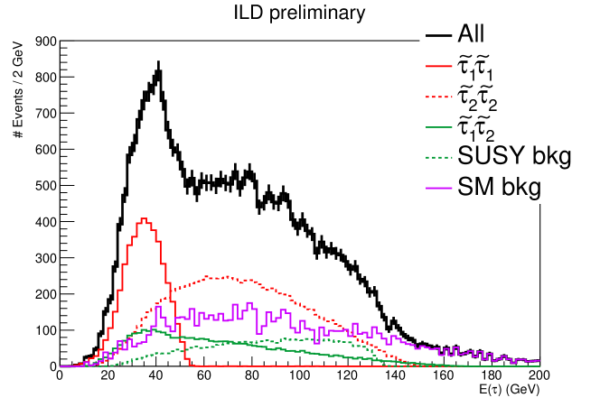
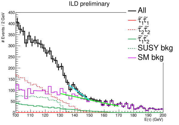
Figure 2: The reconstructed higher $\tau$ energy distribution in an event after applying all selection cuts for eLpR beam polarization. The vertical error bars correspond to the expected statistical uncertainty in the actual running.

(a) $\tilde{\tau}_{2}\tilde{\tau}_{2}$ endpoint fit

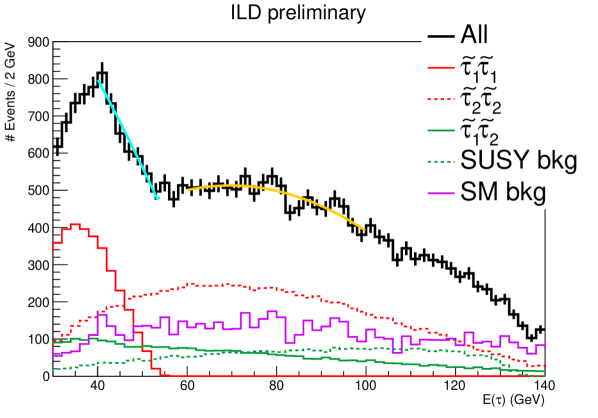
(b) $\tilde{\tau}_{1}\tilde{\tau}_{1}$ endpoint fit

Figure 3: Zoomed regions of Fig. 3. (a) The $\tilde{\tau}_{2}\tilde{\tau}_{2}$ endpoint region. The light green and cyan lines correspond to the SM background fit and the fit of all the events, respectively. (b) The $\tilde{\tau}_{1}\tilde{\tau}_{1}$ endpoint region. The cyan (yellow) line is the fit result of all the events for the $E_{\tau}$ range of 40–$54\,\mathrm{GeV}$ (60–$100\,\mathrm{GeV}$). See text for details of the fittings.

Let us begin with the eLpR beam configuration. We first extract the endpoint $E_{+}(\tilde{\tau}_{2})$ from the pair-production process $e^{+}e^{-}\rightarrow\tilde{\tau}_{2}^{*}\tilde{\tau}_{2}$. In Fig. 3 (a), we show the energy distribution of $E_{\tau}$ as well as the results of the fits in the signal and background regions. In the present case, the effect of the SUSY backgrounds is expected to be small because, at $E_{\tau}\sim E_{+}(\tilde{\tau}_{2})$, the SUSY event is dominated by the $\tilde{\tau}_{2}^{*}\tilde{\tau}_{2}$ pair-production event. On the contrary, the SM background is substantial. We assume that, at the time of the ILC operation, the SM background for the extraction of $E_{+}(\tilde{\tau}_{2})$ will be well understood by combining the side-band data and the MC analysis and that the endpoint can be determined by comparing the real data with the SM background. In the present analysis, the would-be-known SM background is estimated from the MC result shown in Fig. 3 (a); we use the SM background distribution given by the straight line determined from our MC data in the range of 130–170 GeV (the light green line). We then perform fitting for all the events using an additional straight line on the SM fit in the range of 136–150 GeV (the cyan line). We can extract the endpoint as the crossover of these lines. Then, we obtain

$$E_{+}(\tilde{\tau}_{2})=149.5\pm 1.7\,\mathrm{GeV}\,,$$ (19)

consistent with the theoretical endpoint value 149.9 GeV.

The $\tilde{\tau}_{1}$ endpoint is also extracted as shown in Fig. 3 (b). We first fit the distribution of all the events using a second-order polynomial in the range of 60–100 GeV (the yellow line) for the estimation of the background. Here we do not assume that the contributions from the $\tilde{\tau}_{1}\tilde{\tau}_{2}$ and $\tilde{\tau}_{2}\tilde{\tau}_{2}$ processes are known, since they depend on the yet-unknown stau mixing parameter. This treatment allows to regard this procedure as a data-driven estimation of the background. We then in the range 40–54 GeV perform a fit (the cyan line) by a linear function stacked on the extrapolation of the aforementioned second-order polynomial fit function. The obtained endpoint for $\tilde{\tau}_{1}$ is

$$E_{+}(\tilde{\tau}_{1})=53.31\pm 0.55\,\mathrm{GeV}\,,$$ (20)

which is smaller than the theoretical endpoint 54.5 GeV.

For extracting the stau cross section, we use the number of events in the energy range $60\,\mathrm{GeV}<E_{\tau}<150\,\mathrm{GeV}$. For an integrated luminosity ${\cal L}=1.6\,\mathrm{ab^{-1}}$ for eLpR beam polarization, the expected number of signal and background events in this range are found to be

$$N_{22} =6413\,,$$ (21)

$$N_{12} =1705\,,$$ (22)

$$N_{\text{SM}} =4873\,,$$ (23)

$$N_{\text{SUSY}} =2365\,,$$ (24)

where $N_{22}$, $N_{12}$, $N_{\text{SM}}$, and $N_{\text{SUSY}}$ are the numbers of events of $\tilde{\tau}_{2}\tilde{\tau}_{2}$ production, $\tilde{\tau}_{1}\tilde{\tau}_{2}$ production, SM background, and SUSY background, respectively.

3.2.2 Measurements with eRpL Polarization

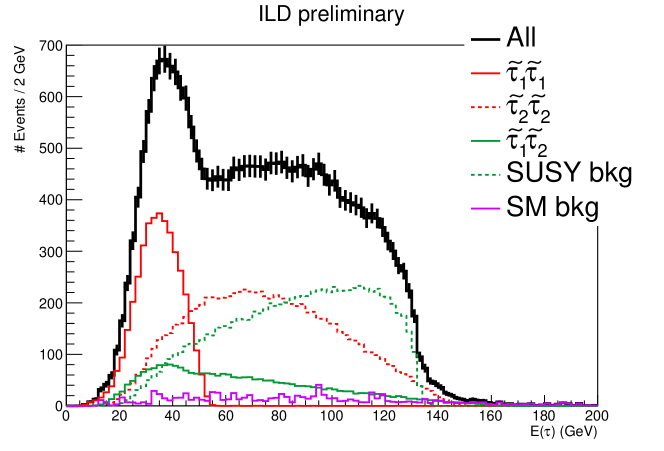
Figure 4: The reconstructed higher $\tau$ energy distribution in an event after applying all selection cuts for eRpL beam polarization. The vertical error bars correspond to the expected statistical uncertainty in the actual running.

(a) $\tilde{\tau}_{2}\tilde{\tau}_{2}$ endpoint fit

(b) $\tilde{\tau}_{1}\tilde{\tau}_{1}$ endpoint fit

Figure 5: Zoomed regions of Fig. 5. (a) The $\tilde{\tau}_{2}\tilde{\tau}_{2}$ endpoint region. The light green and cyan lines correspond to the SM background fit and the fit of all the events, respectively. (b) The $\tilde{\tau}_{1}\tilde{\tau}_{1}$ endpoint region. The cyan (yellow) line is the fit result of all the events for the $E_{\tau}$ range of 40–$54\,\mathrm{GeV}$ (60–$100\,\mathrm{GeV}$). See text for details of the fittings.

We repeat the aforementioned analysis for the eRpL beam configuration. The resulting $E_{\tau}$ distribution is shown in Fig. 5. As displayed in Fig. 5, the $\tilde{\tau}_{2}$ endpoint is obtained as

$$E_{+}(\tilde{\tau}_{2})=150.4\pm 1.2\,\mathrm{GeV}\,,$$ (25)

which is consistent with the theoretical endpoint value 149.9 GeV, and the $\tilde{\tau}_{1}$ endpoint is

$$E_{+}(\tilde{\tau}_{1})=53.17\pm 0.67\,\mathrm{GeV}\,,$$ (26)

which is slightly smaller than the theoretical endpoint 54.5 GeV.

For an integrated luminosity ${\cal L}=1.6\,\mathrm{ab^{-1}}$ for eRpL beam polarization, the expected number of signal and background events in the range $60\,\mathrm{GeV}<E_{\tau}<150\,\mathrm{GeV}$ are found to be

$$N_{22} =5803\,,$$ (27)

$$N_{12} =1354\,,$$ (28)

$$N_{\text{SM}} =595.2\,,$$ (29)

$$N_{\text{SUSY}} =7215\,.$$ (30)

3.3 Fit of Stau Masses and Mixing Angle

In this section, we fit the stau masses and the mixing angle from the values of the endpoints and the expected number of signal events simultaneously. We define the following $\chi^{2}$ variable:

$$\chi^{2}_{\mathrm{tot}}(m_{\tilde{\tau}_{1}},m_{\tilde{\tau}_{2}},\cos\theta_{\tilde{\tau}},m_{\tilde{\chi}_{1}^{0}})=\chi^{2}_{m_{\tilde{\chi}_{1}^{0}}}+\sum_{\text{pol.}}\left[\chi^{2}_{E_{+}(\tilde{\tau}_{1})}+\chi^{2}_{E_{+}(\tilde{\tau}_{2})}+\chi^{2}_{N(\tilde{\tau})}\right]\,,$$ (31)

where the polarization (pol.) sum runs over the eLpR and eRpL polarization configurations and $\chi^{2}_{\mathcal{O}}$ for each observable $\mathcal{O}$ is given by

$$\chi^{2}_{\mathcal{O}}\equiv\frac{(\mathcal{O}^{\rm th}-\mathcal{O}^{\rm exp})^{2}}{\sigma_{\mathcal{O}}^{2}}$$ (32)

with $\mathcal{O}^{\rm th}$ and $\mathcal{O}^{\rm exp}$ being theoretically predicted and experimentally observed values, respectively, and $\sigma_{\mathcal{O}}^{2}$ being the variance. Here, $\chi^{2}_{m_{\tilde{\chi}_{1}^{0}}}$ and $\chi^{2}_{N(\tilde{\tau})}$ are for the LSP mass and the number of the stau events, respectively. We neglect the correlation among different observables. Using the $\chi^{2}$ variable, the probability distribution function (PDF) is defined as ${\cal P}\propto e^{-\chi^{2}_{\mathrm{tot}}/2}$.

For the calculation of $\chi^{2}_{m_{\tilde{\chi}_{1}^{0}}}$, we use $m_{\tilde{\chi}^{0}_{1}}^{\rm exp}=99.3\,\mathrm{GeV}$ and $\sigma_{m_{\tilde{\chi}^{0}_{1}}}=0.1\,\mathrm{GeV}$, where the former comes from the true value in the model point (see Table 1) and the latter, associated to an endpoint search in the process $e^{+}e^{-}\to\tilde{\mu}^{+}\tilde{\mu}^{-}/\tilde{e}^{+}\tilde{e}^{-}$, is adopted from Refs. [33, 10]. Theoretical values of the endpoints for $\chi^{2}_{E_{+}(\tilde{\tau}_{1})}$ and $\chi^{2}_{E_{+}(\tilde{\tau}_{2})}$ are given by Eq. (17) with $E_{\tilde{\tau}_{i}}=\sqrt{s}/2$, while $E_{+}(\tilde{\tau}_{i})^{\rm exp}$’s are taken from Eqs. (20) and (26) for $i=1$ and Eqs. (19) and (25) for $i=2$.

For the calculation of $\chi^{2}_{N(\tilde{\tau})}$, we utilize the number of events, Eqs. (21)–(24) and Eqs. (27)–(30) for eLpR and eRpL polarization configurations, respectively. There, we imposed an additional cut, $60\,\mathrm{GeV}<E_{\tau}<150\,\mathrm{GeV}$, to collect $\tilde{\tau}_{1}\tilde{\tau}_{2}$ and $\tilde{\tau}_{2}\tilde{\tau}_{2}$ events. This cut eliminates $\tilde{\tau}_{1}\tilde{\tau}_{1}$ events and makes the number of events more sensitive to the stau mixing angle. We construct $\chi^{2}_{N(\tilde{\tau})}$ with

$$N(\tilde{\tau})^{\rm th} =\mathcal{L}\left[2\epsilon_{12}\,\sigma(e^{+}e^{-}\to\tilde{\tau}_{1}^{\ast}\tilde{\tau}_{2})+\epsilon_{22}\,\sigma(e^{+}e^{-}\to\tilde{\tau}_{2}^{\ast}\tilde{\tau}_{2})\right]\,,$$ (33)

$$N(\tilde{\tau})^{\rm exp} =N_{\rm total}-N_{\rm bkg}\,,$$ (34)

$$\sigma_{N(\tilde{\tau})} =\sqrt{N_{\rm total}+N_{\rm bkg}}\,.$$ (35)

Here, we first evaluate the signal efficiencies ($\epsilon_{12}$ and $\epsilon_{22}$) by comparing the MC result in the range of $60\,\mathrm{GeV}<E_{\tau}<150\,\mathrm{GeV}$ with the theoretical cross section in Eq. (9). It is assumed that the signal efficiencies are insensitive to the stau mixing angle and masses. The number of total events in the range of $60\,\mathrm{GeV}<E_{\tau}<150\,\mathrm{GeV}$ is $N_{\rm total}$, which will be given by experiment, and we use $N_{\rm total}=N_{\rm signal}+N_{\rm bkg}$ and $N_{\rm signal}=N_{12}+N_{22}$. The number of background events, $N_{\rm bkg}=N_{\text{SUSY}}+N_{\text{SM}}$, will be determined by the MC analysis.

Note that $\chi^{2}_{N(\tilde{\tau})}$ has a twofold ambiguity with regard to the stau mixing angle $\theta_{\tilde{\tau}}$. Since the slepton pair-production cross section in Eq. (9) is invariant under $\theta_{\tilde{l}}\leftrightarrow(\pi-\theta_{\tilde{l}})$, we cannot resolve this degeneracy. This degeneracy corresponds to the sign of the $\mu$ parameter. The sign of the muon $g-2$ anomaly implies $\mu M_{1}>0$. Therefore, this degeneracy also corresponds to the sign of $M_{1}$. In our fitting, we assumed $\mu>0$ with $M_{1}>0$.

Using the PDF, ${\cal P}\propto e^{-\chi^{2}_{\mathrm{tot}}/2}$, we obtain

$$m_{\tilde{\tau}_{1}} =112.8\pm 0.2\,\mathrm{GeV}\,,$$ (36)

$$m_{\tilde{\tau}_{2}} =189.9_{-0.7}^{+0.8}\,\mathrm{GeV}\,,$$ (37)

$$\cos\theta_{\tilde{\tau}} =0.703\pm 0.010\,,$$ (38)

with $68\%$ probability ranges. Here, we require that both edges of the uncertainty have the same value of the PDF. From Eq. (7), the stau left-right mixing parameter is given by

$$-m_{\tilde{\tau}{LR}}^{2}=\left(1.17\pm 0.01\right)\times 10^{4}\,\mathrm{GeV}{}^{2}\,.$$ (39)

Then the smuon left-right mixing parameter can be reconstructed from Eq. (4) as

$$-m_{\tilde{\mu}{LR}}^{2}=693_{-8}^{+9}\,\mathrm{GeV}{}^{2}\,.$$ (40)

All the fitted values and the corresponding theoretical values at the benchmark point are summarized in Table 4.

Table 4: Fitting summary for the stau parameters with $\sqrt{s}=500\,\mathrm{GeV}$ and ${\cal L}=1.6\,\mathrm{ab^{-1}}$. The mass parameters are in units of GeV and the left-right mixing parameter is in units of GeV².

	$m_{\tilde{\tau}_{1}}$	$m_{\tilde{\tau}_{2}}$	$\cos\theta_{\tilde{\tau}}$	$-m_{\tilde{\tau}{LR}}^{2}$
Theoretical value	113.2	189.8	0.703	11606
Fit result	$112.8\pm 0.2$	$189.9_{-0.7}^{+0.8}$	$0.703\pm 0.010$	$\left(1.17\pm 0.01\right)\!\times\!10^{4}$

4 Reconstruction of the Muon $g-2$

In this section, we study an implication of the determinations of stau parameters, in particular $m_{\tilde{\tau}{LR}}^{2}$, for the muon $g-2$ anomaly. We discuss how accurately the SUSY contribution to ${a_{\mu}}$ is determined using the ILC measurements at our benchmark point. It is assumed that all the charged sleptons and the lightest neutralino (as the LSP) are within the kinematical reach of the ILC and that no other superparticles, in particular charginos, are discovered. In such a case, the neutralino can be considered as the Bino-dominated one. Furthermore, in the absence of the chargino discovery, we may expect that the SUSY contribution to the muon $g-2$ is dominated by the Bino-smuon loop contribution $a_{\mu}^{(\tilde{B})}$.

We can reconstruct $a_{\mu}^{(\tilde{B})}$ once the following quantities are known:

• Smuon mass eigenvalues: $m_{\tilde{\mu}_{1}}$ and $m_{\tilde{\mu}_{2}}$,

• Smuon left-right mixing parameter: $m_{\tilde{\mu}{LR}}^{2}$,

• The lightest neutralino mass: $m_{\tilde{\chi}^{0}_{1}}$.

At the ILC, the smuon masses can be measured from the smuon pair-production processes, and the lightest neutralino mass can be done from the selectron production processes in addition to the smuon ones. As for the smuon left-right mixing parameter $m_{\tilde{\mu}{LR}}^{2}$, as we have discussed, the stau study at the ILC can be used for its determination. It is obtained from the stau left-right mixing parameter (see Eq. (4)). Once $m_{\tilde{\mu}{LR}}^{2}$ and the smuon masses are known, the smuon mixing angle $\theta_{\tilde{\mu}}$ is determined from the relation,

$$\sin 2\theta_{\tilde{\mu}}=\frac{2m_{\tilde{\mu}{LR}}^{2}}{m_{\tilde{\mu}_{1}}^{2}-m_{\tilde{\mu}_{2}}^{2}}=\frac{m_{\mu}}{m_{\tau}}\frac{m_{\tilde{\tau}_{2}}^{2}-m_{\tilde{\tau}_{1}}^{2}}{m_{\tilde{\mu}_{2}}^{2}-m_{\tilde{\mu}_{1}}^{2}}\sin 2\theta_{\tilde{\tau}}\,,$$ (41)

with which the smuon mixing matrix $U_{\tilde{\mu}}$ is obtained.

With the above mentioned parameters, the Bino-smuon contribution to ${a_{\mu}^{\mathrm{SUSY}}}$ can be calculated. At the one-loop level, it is given by

$$a_{\mu}^{(\tilde{B},{\rm\ 1\mathchar 45\relax loop})}= \frac{1}{16\pi^{2}}\sum_{A=1,2}\frac{m_{\mu}^{2}}{m_{\tilde{\mu}_{A}}^{2}}\left\{-\frac{1}{12}\left[(\hat{N}^{\mu_{L}}_{A})^{2}+(\hat{N}^{\mu_{R}}_{A})^{2}\right]F^{N}_{1}\left(\frac{m_{\tilde{\chi}^{0}_{1}}^{2}}{m_{\tilde{\mu}_{A}}^{2}}\right)\right.$$

$$\qquad\qquad\qquad\quad~{}~{}\left.-\frac{m_{\tilde{\chi}^{0}_{1}}}{3m_{\mu}}\hat{N}^{\mu_{L}}_{A}\hat{N}^{\mu_{R}}_{A}F^{N}_{2}\left(\frac{m_{\tilde{\chi}^{0}_{1}}^{2}}{m_{\tilde{\mu}_{A}}^{2}}\right)\right\}\,,$$ (42)

where

$$\hat{N}^{\mu_{L}}_{A}=\frac{1}{\sqrt{2}}g_{Y}(U_{\tilde{\mu}})_{A1}\,,\qquad\hat{N}^{\mu_{R}}_{A}=-\sqrt{2}g_{Y}(U_{\tilde{\mu}})_{A2}\,,$$ (43)

with $g_{Y}$ being the U(1)_Y gauge coupling constant, and the loop functions are defined as

$$F^{N}_{1}(x) =\frac{2}{(1-x)^{4}}\left(1-6x+3x^{2}+2x^{3}-6x^{2}\ln x\right)\,,$$ (44)

$$F^{N}_{2}(x) =\frac{3}{(1-x)^{3}}\left(1-x^{2}+2x\ln x\right)\,.$$ (45)

In our analysis, we include the photonic correction to evaluate $a_{\mu}^{(\tilde{B})}$ as

$$a_{\mu}^{(\tilde{B})}=a_{\mu}^{(\tilde{B},{\rm\ 1\mathchar 45\relax loop})}+a_{\mu}^{(\tilde{B},{\rm\ photonic})},$$ (46)

where $a_{\mu}^{(\tilde{B},{\rm\ photonic})}$ is the two-loop photonic contribution [20].

The stau study of the ILC can give crucial information for the reconstruction of $a_{\mu}^{(\tilde{B})}$ through the determination of $m_{\tilde{\mu}{LR}}^{2}$. To understand the impact of the stau study, let us estimate the uncertainty related to $m_{\tilde{\mu}{LR}}^{2}$ in the reconstructed value of $a_{\mu}^{(\tilde{B})}$. Including only the uncertainty in Eq. (40), we obtain

$$\left.a_{\mu}^{(\tilde{B})}\right|_{m_{\tilde{\mu}{LR}}^{2}}=(27.6\pm 0.3)\times 10^{-10}\quad[\pm 1\%]\,.$$ (47)

With including all the uncertainties, $a_{\mu}^{(\tilde{B})}$ is reconstructed as

$$a_{\mu}^{(\tilde{B})}=(27.5\pm 0.4)\times 10^{-10}\quad[\pm 1\%]\,,$$ (48)

where the uncertainties on $m_{\tilde{\mu}_{1}}$, $m_{\tilde{\mu}_{2}}$, and $m_{\tilde{\chi}^{0}_{1}}$ are taken to be $0.2\,\mathrm{GeV}$, $0.2\,\mathrm{GeV}$, and $0.1\,\mathrm{GeV}$, respectively [10]. At the benchmark point of our choice, the uncertainty in the reconstructed value of $a_{\mu}^{(\tilde{B})}$ is dominated by the one related to the smuon left-right mixing parameter $m_{\tilde{\mu}{LR}}^{2}$. It is concluded that the stau study at the ILC can help reconstructing $a_{\mu}^{(\tilde{B})}$ at the $1\%$ accuracy. Improvements of the measurements of the stau parameters can reduce the uncertainty, which may become possible with an ILC operation with higher luminosity or larger beam energy.

5 Summary

The Fermilab experiment result confirmed the long-standing muon $g-2$ anomaly. If the muon $g-2$ anomaly mainly comes from the Bino contribution in SUSY models, $\Delta a_{\mu}\simeq{a_{\mu}^{\mathrm{SUSY}}}\simeq a_{\mu}^{(\tilde{B})}$, and if all the sleptons and the lightest neutralino are within the kinematical reach, the ILC will be able to measure the MSSM parameters which are necessary to estimate $a_{\mu}^{(\tilde{B})}$. In this work, we have investigated the measurements of the stau masses and mixing at the ILC, which are essential ingredients to determine the $a_{\mu}^{(\tilde{B})}$. We have also discussed their implication for the $a_{\mu}^{(\tilde{B})}$ reconstruction. We have shown that, at our benchmark point, the SUSY contribution to the muon $g-2$ can be reconstructed with the accuracy of $\sim 1\%$ at the ILC with $\sqrt{s}=500$ GeV and an integrated luminosity ${\cal L}=1.6\,\mathrm{ab^{-1}}$.

References

- [1] Muon g-2 Collaboration, “Measurement of the positive muon anomalous magnetic moment to 0.7 ppm,” Phys. Rev. Lett. 89 (2002) 101804 [hep-ex/0208001].
- [2] Muon g-2 Collaboration, “Measurement of the negative muon anomalous magnetic moment to 0.7 ppm,” Phys. Rev. Lett. 92 (2004) 161802 [hep-ex/0401008].
- [3] Muon g-2 Collaboration, “Final Report of the Muon E821 Anomalous Magnetic Moment Measurement at BNL,” Phys. Rev. D73 (2006) 072003 [hep-ex/0602035].
- [4] Muon g-2 Collaboration, “Measurement of the Positive Muon Anomalous Magnetic Moment to 0.46 ppm,” Phys. Rev. Lett. 126 (2021) 141801 [arXiv:2104.03281].
- [5] T. Aoyama et al., “The anomalous magnetic moment of the muon in the Standard Model,” Phys. Rept. 887 (2020) 1–166 [arXiv:2006.04822].
- [6] M. Endo, K. Hamaguchi, S. Iwamoto, and T. Kitahara, “Supersymmetric interpretation of the muon anomaly,” JHEP 07 (2021) 075 [arXiv:2104.03217].
- [7] J. L. Lopez, D. V. Nanopoulos, and X. Wang, “Large in SU(5) U(1) Supergravity Models,” Phys. Rev. D49 (1994) 366–372 [hep-ph/9308336].
- [8] U. Chattopadhyay and P. Nath, “Probing Supergravity Grand Unification in the Brookhaven Experiment,” Phys. Rev. D53 (1996) 1648–1657 [hep-ph/9507386].
- [9] T. Moroi, “The Muon anomalous magnetic dipole moment in the minimal supersymmetric standard model,” Phys. Rev. D53 (1996) 6565–6575 [hep-ph/9512396] [Erratum ibid. D56 (1997) 4424].
- [10] M. Endo, K. Hamaguchi, S. Iwamoto, T. Kitahara, and T. Moroi, “Reconstructing Supersymmetric Contribution to Muon Anomalous Magnetic Dipole Moment at ILC,” Phys. Lett. B 728 (2014) 274–281 [arXiv:1310.4496].
- [11] M. M. Nojiri, “Polarization of lepton from scalar decay as a probe of neutralino mixing,” Phys. Rev. D 51 (1995) 6281–6291 [hep-ph/9412374].
- [12] E. Boos, et al., “Polarization in sfermion decays: Determining tan beta and trilinear couplings,” Eur. Phys. J. C 30 (2003) 395–407 [hep-ph/0303110].
- [13] M. M. Nojiri, K. Fujii, and T. Tsukamoto, “Confronting the minimal supersymmetric standard model with the study of scalar leptons at future linear e+ e- colliders,” Phys. Rev. D 54 (1996) 6756–6776 [hep-ph/9606370].
- [14] P. Bechtle, M. Berggren, J. List, P. Schade, and O. Stempel, “Prospects for the study of the -system in SPS1a’ at the ILC,” Phys. Rev. D 82 (2010) 055016 [arXiv:0908.0876].
- [15] M. Berggren, et al., “Non-simplified SUSY: -coannihilation at LHC and ILC,” Eur. Phys. J. C 76 (2016) 183 [arXiv:1508.04383].
- [16] S. Marchetti, S. Mertens, U. Nierste, and D. Stockinger, “Tan(beta)-enhanced supersymmetric corrections to the anomalous magnetic moment of the muon,” Phys. Rev. D 79 (2009) 013010 [arXiv:0808.1530].
- [17] J. Girrbach, S. Mertens, U. Nierste, and S. Wiesenfeldt, “Lepton flavour violation in the MSSM,” JHEP 05 (2010) 026 [arXiv:0910.2663].
- [18] T. Kitahara and T. Yoshinaga, “Stau with Large Mass Difference and Enhancement of the Higgs to Diphoton Decay Rate in the MSSM,” JHEP 05 (2013) 035 [arXiv:1303.0461].
- [19] M. Endo, K. Hamaguchi, T. Kitahara, and T. Yoshinaga, “Probing Bino contribution to muon ,” JHEP 11 (2013) 013 [arXiv:1309.3065].
- [20] P. von Weitershausen, M. Schafer, H. Stockinger-Kim, and D. Stockinger, “Photonic SUSY Two-Loop Corrections to the Muon Magnetic Moment,” Phys. Rev. D 81 (2010) 093004 [arXiv:1003.5820].
- [21] G. Degrassi and G. F. Giudice, “QED logarithms in the electroweak corrections to the muon anomalous magnetic moment,” Phys. Rev. D 58 (1998) 053007 [hep-ph/9803384].
- [22] W. Kilian, T. Ohl, and J. Reuter, “WHIZARD: Simulating Multi-Particle Processes at LHC and ILC,” Eur. Phys. J. C 71 (2011) 1742 [arXiv:0708.4233].
- [23] Shin-ichi Kawada, “The mini-DST: a high-level LCIO format.” arXiv:2105.08622.
- [24] M. Chrzaszcz, T. Przedzinski, Z. Was, and J. Zaremba, “TAUOLA of lepton decays—framework for hadronic currents, matrix elements and anomalous decays,” Comput. Phys. Commun. 232 (2018) 220–236 [arXiv:1609.04617].
- [25] DELPHES 3 Collaboration, “DELPHES 3, A modular framework for fast simulation of a generic collider experiment,” JHEP 02 (2014) 057 [arXiv:1307.6346].
- [26] “ILCDelphes.” https://github.com/iLCSoft/ILCDelphes.
- [27] The ILD Concept Group, “International Large Detector: Interim Design Report.” arXiv:2003.01116.
- [28] M. Berggren, “SGV 3.0 - a fast detector simulation,” in International Workshop on Future Linear Colliders (LCWS11). 2012. arXiv:1203.0217. Available at https://svnsrv.desy.de/public/sgv/trunk/.
- [29] J. S. Marshall and M. A. Thomson, “Pandora Particle Flow Algorithm,” in Proceedings, International Conference on Calorimetry for the High Energy Frontier (CHEF 2013): Paris, France, April 22–25, 2013, pp. 305–315. 2013. arXiv:1308.4537.
- [30] “TauFinder.” https://github.com/iLCSoft/MarlinReco/tree/master/Analysis/TauFinder.
- [31] T. Barklow, et al., “ILC Operating Scenarios.” arXiv:1506.07830.
- [32] LCC Physics Working Group, “Physics Case for the 250 GeV Stage of the International Linear Collider.” arXiv:1710.07621.
- [33] H.-U. Martyn, “Detection of sleptons at a linear collider in models with small slepton-neutralino mass differences,” in International Conference on Linear Colliders (LCWS 04). 2004. hep-ph/0408226.