COP: Control & Observability-aware Planning

Abstract

In this research, we aim to answer the question: How to combine Closed-Loop State and Input Sensitivity-based with Observability-aware trajectory planning? These possibly opposite optimization objectives can be used to improve trajectory control tracking and, at the same time, estimation performance.

Our proposed novel Control & Observability-aware Planning (COP) framework is the first that uses these possibly opposing objectives in a Single-Objective Optimization Problem (SOOP) based on the Augmented Weighted Tchebycheff method to perform the balancing of them and generation of Bézier curve-based trajectories. Statistically relevant simulations for a 3D quadrotor unmanned aerial vehicle (UAV) case study produce results that support our claims and show the negative correlation between both objectives. We were able to reduce the positional mean integral error norm as well as the estimation uncertainty with the same trajectory to comparable levels of the trajectories optimized with individual objectives.

I Introduction

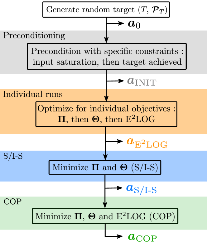
Figure 1: Graphic overview of the multi-step Single-Objective Optimization Problem (SOOP) solved with Control & Observability-aware Planning (COP), $\bm{a}_{i}$ being the resulting trajectory coefficients after each operation.

I-A Motivation & Related Work

Motion planning algorithms are a crucial component of autonomous task execution for an UAV or robots in general.

I-A1 Trajectory Generation

A common approach is to generate a series of way-points in discrete time intervals - a so-called trajectory. These trajectories are often 4D flat outputs (3D position and yaw orientation) of the UAV with their subsequent derivatives. These generation methods often let the UAV move from point A to point B with additional goals and constraints, e.g., reducing flight time or energy consumption. Examples of such generation methods based on continuous-space models can be found in [1, 2, 3, 4], acting on different levels of abstraction and even taking probabilities into account. [5, 6, 7, 8] create a discrete map of the task-space, a so-called sampling-based method, to apply search algorithms to find a path from A to B. With the increase of computational power, learning-based approaches attracted attention in recent years. [9, 10, 11] use machine learning for trajectory generation with reduced calculation times.

All previously mentioned approaches do not consider model and state uncertainties to ensure robust trajectory tracking or accurate state/parameter estimation.

I-A2 Estimation-aware Trajectories

State estimation with proper system modeling [12] relies on the design of sufficiently informative system input for accurate and fast estimate convergence. The works in [13, 14, 15, 16, 17, 18, 19] show that taking the estimation or parametric uncertainty into account drastically improves system parameter estimation results while allowing task execution. In this work we will use the Expanded Empirical Local Observability Gramian (E²LOG) [14]. These informative trajectories might show poor robustness against uncertainties in the robot model for the tracking controller that executes them [20, 21].

I-A3 Control-aware Trajectories

To address this issue, the notion of Closed-Loop State and Input Sensitivities (S/I-S) has been recently introduced in [22, 23] as a suitable metric to be optimized. Minimizing the norm of the S/I-S generates a trajectory whose tracking results are minimally sensitive to model uncertainties of the robot states and inputs. This is important as it increases the robustness and accuracy of the trajectory tracking and improves the repeatability of the control inputs when the model parameters vary. The S/I-S, however, needs knowledge of the actual robot state and nominal values of the model parameters, which may not be directly available but can be provided by state estimation.

I-A4 Link & Combination

Therefore, a link between observability-related metrics and S/I-S metrics exists, since the evaluation of S/I-S needs a good knowledge of states and parameters, and the tracking of maximally observable trajectories benefits from increased robustness in the trajectory execution. That fact motivates our study on how to combine both methods in a unified trajectory optimization problem taking into account that these two objectives can conflict among themselves, as seen in Sec. IV.

I-B Contributions

This paper proposes Control & Observability-aware Planning (COP) as a way to balance two possibly contradicting optimization problems, namely $(i)$ generating trajectories whose execution is minimally sensitive to model uncertainties and $(ii)$ generating trajectories that can be sufficiently informative for accurate state estimation. We present a method to address these problems by leveraging previous contributions to the topics of observability-aware and minimally-sensitive trajectory planning, combining them in the formulation and resolution of a Single-Objective Optimization Problem (SOOP) based on the Augmented Weighted Tchebycheff method. In a case study, considering the state estimation and robust trajectory tracking for a 3D quadrotor UAV, we discuss the statistical results of a realistic simulation campaign that shows the potential of the proposed contribution.

II Preliminaries

II-A Quadrotor model

Let us consider a frame $\mathcal{M}$ as the quadrotor body frame, attached to its center of mass (CoM), with its z-axis $\bm{z}_{M}$ aligned with the thrust of the four rotors. The state vector $\mathbf{x}$ of this system consists of its linear position $\bm{r}=(x,\,y,\,z)$ and velocity $\bm{v}=(v_{x},\,v_{y},\,v_{z})$, both expressed in the world frame $\mathcal{W}$. It also includes the body orientation expressed through the unit length quaternion $\bm{q}=(q_{w},\,q_{x},\,q_{y},\,q_{z})$ (Tait–Bryan angle definition with yaw first (312-sequence)) as well as its angular velocity $\bm{\omega}=(\omega_{x},\,\omega_{y},\,\omega_{z})$, expressed in the body frame $\mathcal{M}$, therefore $\mathbf{x}=\left[\bm{r}^{\mathsf{T}},\bm{v}^{\mathsf{T}},\bm{q}^{\mathsf{T}},\bm{\omega}^{\mathsf{T}}\right]^{\mathsf{T}}\in\mathbb{R}^{13}$.

As the quadrotor’s orientation is expressed by the Hamiltonian quaternion $\bm{q}$, we recall that $\bm{z}_{M}=\mathbf{R}(\bm{q})\bm{z}_{W}=\bm{q}^{-1}\otimes\bm{z}_{W}\otimes\bm{q}$, where $\otimes$ is the quaternion product. $\mathbf{R}(\bm{q})$ is the rotation matrix as a function of the quaternion $\mathbf{q}$.

It is possible to link the squared rotor speeds of the quadrotor (control inputs) $\mathbf{u}=\left[\omega_{1}^{2}\ \omega_{2}^{2}\ \omega_{3}^{2}\ \omega_{4}^{2}\right]^{\mathsf{T}}$ to $[f,\,\bm{\tau}^{\mathsf{T}}]^{\mathsf{T}}$, the total effective thrust and torque. These are related by the allocation matrix $\bm{S}$, $[f,\,\bm{\tau}^{\mathsf{T}}]^{\mathsf{T}}=\bm{S}\mathbf{u}$ (e.g., [24] Eq. (8)), which includes the rotor thrust force coefficient $k_{f}$, the drag moment coefficient $k_{m}$, and the arm length $\ell$ from the center of mass to each motor/rotor group.

With these definitions, compared to [22], the quadrotor dynamical model is

$$\dot{\mathbf{x}}=\left\{\begin{aligned} \bm{\dot{r}}_{W}&=\bm{v}_{W}\\ \bm{\dot{v}}_{W}&=-g\bm{z}_{W}+\tfrac{f}{m}\bm{z}_{M}\\ \bm{\dot{q}}&=\tfrac{1}{2}\bm{q}\otimes\omega_{M}\\ \bm{\dot{\omega}}_{M}&=\bm{J}^{-1}(\bm{\tau}-\bm{\omega}_{M}\times(\bm{J}\bm{\omega}_{M}))\end{aligned}\right.$$ (1)

where $m$ and $\bm{J}$ are the quadrotor’s mass and its inertia matrix, respectively. $g$ is the Earth’s gravitational pull. The allocation matrix $\bm{S}$ implies that the dynamics are also effected by the parameters $k_{f}$, $k_{m}$ and $\ell$. The quantities $k_{f}$ and $k_{m}$ are aerodynamic parameters that depend on the rotors characteristics and the aerodynamic interaction with the environment (e.g., presence of wind, ground effects). Therefore, an accurate value for these parameters can be hard to obtain, and we thus consider $\mathbf{p}=\left[k_{f}\ k_{m}\right]^{T}\in\mathbb{R}^{2}$ as the uncertain parameters of the dynamical model.

II-B Tracking controller

With the dynamic model detailed in the previous subsection, we can now present the controller that has been used in this work. The chosen control task is to let the system output $\bm{y}(\mathbf{x})=\left[x\ y\ z\ \varphi\right]^{\mathsf{T}}\in\mathbb{R}^{4}$ track a desired motion $\bm{r}_{d}(\bm{a},\ t)\in\mathbb{R}^{4}$, where $\varphi$ is the yaw (or heading) angle of the quadrotor. The DFL (Dynamic Feedback Linearization) controller with an integral term used in previous works [23, 22] is not robust against parameter uncertainties and is not capable of considering input constraints. Therefore, we chose to use a different controller, namely the so-called Lee controller [20], which performs slightly worse in an ideal case compared to the DFL, but it is much less complex to implement and tune.

Although we implemented the same structure of the controller as in [20], we added some minor changes in order to match the dynamics of the quadrotor in 3D (especially the use of the quaternion $\mathbf{q}$). In particular we consider attitude and angular velocity errors defined as

$$\bm{e}_{\bm{q}}=\dfrac{1}{2}\left(\bm{R}_{d}^{\mathsf{T}}\bm{R}(\bm{q})-\bm{R}(\bm{q})^{\mathsf{T}}\bm{R}_{d}\right)^{\vee}\text{ and }\bm{e}_{\bm{\omega}}=\bm{w}.$$ (2)

The resulting control inputs are then

$$f=\left(-\bm{k}_{r}\bm{e_{r}}-\bm{k}_{v}\bm{e_{v}}-\bm{k}_{i}\bm{\xi}+m(g\bm{z}_{w}+\ddot{\bm{r}}_{d})\right)\cdot\bm{R}(\bm{q})\bm{z}_{w},$$ (3)

$$\bm{\tau}=-\bm{k}_{q}\bm{e_{q}}-\bm{k}_{\omega}\bm{e_{\omega}},$$ (4)

where $\bm{e}_{r}$ and $\bm{e}_{v}$ are the position and velocity errors, and $\bm{\xi}=\left[\xi_{x}\ \xi_{y}\ \xi_{z}\right]^{\mathsf{T}}$ is the position integrator, and $\bm{k}_{r}$, $\bm{k}_{v}$, $\bm{k}_{i}$, $\bm{k}_{q}$, $\bm{k}_{\omega}$ are suitable control gains. We then compute $\bm{u}$ via the inverse of the allocation matrix, $\mathbf{u}=\bm{S}^{-1}[f,\,\bm{\tau}^{\mathsf{T}}]^{\mathsf{T}}$.

II-C Curve representation

The controller is designed to let the quadrotor follow a reference trajectory $\bm{r}_{d}(\bm{a},\ t)$, where $\bm{a}$ is the parameter vector for the chosen class of curve. In [23] ‘plain polynomials’ were used, with the drawback of introducing possible numerical instability during the optimization. Due to this reason, we switched in [22] to the use of Bézier curve representation, as they are more stable from a numerical point of view.

This work goes one step further by implementing piecewise Beziér curves for the trajectory representation to avoid the use of a single high degree Beziér curve as in [22]. An aditional abstraction happens on the parameter vector $\bm{a}$, which now contains way-points (with velocity, acceleration, and even higher order constraints) instead of the control points themselves. These way-points define the curve at the start, end, and in between curve pieces.

Let $\mathcal{B}_{i\in\llbracket 1,\,n\rrbracket}$, with $n\geqslant 1$ number of pieces, be the Bézier curve of degree $d\geqslant 2$ shaping the trajectory ($\mathcal{C}^{d-1}$ continuity). In total, there are $n+1$ way-points $(t_{i},\,\bm{\mathcal{P}}_{i})$, where $t_{i}$ is the time associated to the point $\bm{\mathcal{P}}_{i}\in\mathbb{R}^{n_{\text{dim}}\times n_{\text{jc}}}$, with $n_{\text{dim}}$ the number of dimensions of the trajectory (e.g., $x$, $y$, $z$, and yaw angle), and $n_{\text{jc}}$ the number of joining conditions (e.g., $n_{\text{jc}}=1$ for position only, which means every Bézier curve piece is a straight line segment). The degree $d$ of the Bézier curve, the number of joining conditions $n_{\text{jc}}$ and the number of control points $n_{c}$ are linked by $d=2n_{\text{jc}}-1=n_{c}-1$. With these conditions and the way-points as constraints, one can formulate a linear system of equations that solves for the control points of each Bezièr curve piece.

III Control & Observability-aware Planning

III-A Objectives for Trajectory Optimization

A trajectory $\bm{r}_{d}(\bm{a},t)$ parameterized by the coefficient vector $\bm{a}$, Sec. II-C, can be optimized for different goals by changing its shape. We represent this goal by the so-called utility function $U(\bm{a})$ which, in our case, is a scalar cost to be minimized subject to constraints

$$\underset{\bm{a}}{\text{minimize}} U(\bm{a}),$$ (5)

subject to $$\bm{a}\in\mathcal{A},$$

$$\text{equ. \& inequ. constraints},$$

with $\mathcal{A}$ as the feasible set for the parameter vector.

III-A1 State Sensitivity Metric

The state sensitivity metric as minimization objective was introduced in [25] and is based on a generic robot model $\dot{\mathbf{x}}=\mathbf{f}(\mathbf{x},\,\mathbf{u},\,\mathbf{p})$, where $\mathbf{x}\in\mathbb{R}^{n_{x}}$ is the state vector, $\mathbf{u}\in\mathbb{R}^{n_{u}}$ is the control input vector, and $\mathbf{p}\in\mathbb{R}^{n_{p}}$ the vector of system parameters (which are assumed uncertain). This is combined with a tracking control law $\dot{\bm{\xi}}=\mathbf{g}(\bm{\xi},\,\mathbf{x},\,\bm{r}_{d}(\mathbf{a},\,t),\,\mathbf{p}_{c})$ and $\mathbf{u}=\mathbf{c}(\bm{\xi},\,\mathbf{x},\,\bm{r}_{d}(\mathbf{a},\,t),\,\mathbf{p}_{c})$, where $\bm{\xi}\in\mathbb{R}^{n_{\xi}}$ are the internal controller states (e.g., an integrator), $\mathbf{p}_{c}$ a nominal value for the parameters $\mathbf{p}$, and $\bm{r}_{d}(\mathbf{a},\,t)$ a desired trajectory. The state sensitivity matrix for the closed-loop system (i.e., considering both the robot and chosen control) is defined as

$$\left.\mathbf{\Pi}(t)=\dfrac{\partial\mathbf{x}(t)}{\partial\mathbf{p}}\right|_{\mathbf{p}=\mathbf{p}_{c}}\in\mathbb{R}^{n_{x}\times n_{p}}$$ (6)

representing the variation of the states $\mathbf{x}$ in relation to variations in the parameter vector $\mathbf{p}$, evaluated on the nominal value $\mathbf{p}_{c}$. We refer the reader to [25] for further details.

The integral of the matrix norm of the state sensitivity over the whole trajectory (duration $T$) can be used to reduce the influence of parameter uncertainty on the states.

$$U(\bm{a})=F_{\Pi}(\bm{a})=\int_{0}^{T}||\bm{\Pi}(t)||\,\mathrm{dt}$$ (7)

III-A2 Input Sensitivity Metric

As natural evolution, [22] added to the state sensitivity metric the so-called input sensitivity metric which is defined as

$$\left.\bm{\Theta}(t)=\dfrac{\partial\mathbf{u}(t)}{\partial\mathbf{p}}\right|_{\mathbf{p}=\mathbf{p}_{c}}\in\mathbb{R}^{n_{u}\times n_{p}}$$ (8)

and, similarly to Eq. (6), maps how variations of the parameter vector $\mathbf{p}$ result in variations of the control inputs. The integral of its matrix norm, again, gives us the objective function Eq. (9) which can be used to reshape the trajectory to be less sensitive in its control inputs against parameter uncertainties. Details on the derivations can be found in [22].

$$U(\bm{a})=F_{\Theta}(\bm{a})=\int_{0}^{T}||\bm{\Theta}(t)||\,\mathrm{dt}$$ (9)

Note that it is not possible to compute $\bm{\Pi}(t)$ in closed-form. However, it is possible to obtain a closed-form expression of its dynamics, and other quantities, e.g., $\bm{\Theta}(t)$, can be derived from it. The evolution of ${\mathbf{\Pi}}(t)$ (consequently $\bm{\Theta}(t)$ too) over a time interval $T$ of interest then can be obtained by numerically integrating over time [25, 22]. One of the main hypotheses/key aspects in [25, 22] is to consider that the whole state of the system is known during the tracking of the desired trajectory.

III-A3 Observability Metric

Online state estimation is one way of making the state $\mathbf{x}$ and parameters $\mathbf{p}$ available at run-time [26, 27, 12].

How well such estimates perform depends on the accuracy of the system model and sensors used, but control inputs given to the robot are equally important. The E²LOG [14, 13] works on the idea of the quality of observability, proposed in [28, 29], which evaluates it over a whole trajectory $\bm{r}_{d}(\mathbf{a},\,t)$ with a duration $T$. It uses a $n$-th order Taylor expansion to approximate the Jacobian matrix which models the sensitivity of the measurements with respect to the control inputs, the state and its changes on a small time horizon $H$ ($\widetilde{\mathbf{W}}_{t_{0},H}(\mathbf{a})$ in [14]). Summing all these quality measure segments along the trajectory $\bm{r}_{d}(\mathbf{a},\,t)$ gives us

$$\widetilde{\mathbf{W}}_{\mathcal{O}}(\mathbf{a})=\sum_{k=0}^{N}\widetilde{\mathbf{W}}_{k\Delta t,\Delta t}(\mathbf{a})\in\mathbb{R}^{n_{x}\times n_{x}}$$ (10)

with $\Delta t=\tfrac{T}{N}$ and $N$ the number of trajectory segments.

The objective is to improve the least sensitive state (or combination of states) through the smallest eigenvalue of $\widetilde{\mathbf{W}}_{\mathcal{O}}(\mathbf{a})$. Adding a minus to the smallest eigenvalue makes it usable in a minimization problem as objective function

$$U(\bm{a})=F_{\text{E${}^{2}$LOG}}(\bm{a})=-\sigma_{\min}(\widetilde{\mathbf{W}}_{\mathcal{O}}(\mathbf{a})).$$ (11)

The result is a trajectory with optimum observability properties, improving the states’ convergence by lowering the uncertainty and increasing the overall accuracy.

The estimator in [12] is the base for the derivation of the observability-aware trajectory optimization in our quadrotor UAV case study, Sec. IV.

III-B Multi-Objective Optimization Problem

The problem presented in this work is an example of a Multi-Objective Optimization Problem (MOOP) trying to optimize for different objectives with constraints.

III-B1 Pareto Optimality

Ideally, one would try to find the non-dominated set in the entire feasible set $\mathcal{A}$ for the parameter vector $\bm{a}$, a so-called Pareto optimal set or Pareto front [30, 31, 32, 33, 34, 35]. The term non-dominated or optimal means that the current set does not improve one objective while worsening another. We compute only one point in the Pareto optimal set due to the complexity of the objective functions and the resulting computation times, see Sec. IV-B4.

In [22], Linear Scalarization Problem (LSP) was chosen as a method because it achieved good results in balancing the S/I-S of a 2D quadrotor. LSP combines objective functions to a single cost through a linear weighting of each objective. This is only a feasible option if the Pareto front is convex. To be more specific, in the case of concave Pareto fronts, LSP tends to converge towards extrema solutions, an optimal solution for only one of the objectives. Evenly distributed weights do not produce an evenly distributed representation of the Pareto optimal set. The addition of the observability-awareness through the E²LOG as a third objective is the natural evolution of the approach, however, non-convexity (concavity) is possible with this addition.

III-B2 Augmented Weighted Tchebycheff Method

To solve this issue, we balance the objectives through their distance between the objective value $F_{i}(\bm{a})$ and an aspiration point $F_{i}^{O}$, compared to [22]. This aspiration point $F_{i}^{O}$ is the individual objective’s minimal value from Eq. (5) - called utopia point. Another important point in the Pareto set is the so-called nadir point $F_{i}^{N}=\underset{1\leq j\leq k}{\max}\{F_{i}(\bm{a}_{j}^{O})\}$. It is the largest cost of all objectives with respect to the $j$-th utopia point.

$$U(\bm{a})=\underset{i}{\max}\{\lambda_{i}|F_{i}(\bm{a})-F_{i}^{O}|\}+\rho\sum_{j=1}^{k}|F_{j}(\bm{a})-F_{j}^{O}|$$ (12)

The utility function in Eq. (12) includes $\mathbf{F}(\bm{a})=\{F_{\Pi}(\bm{a}),F_{\Theta}(\bm{a}),F_{\text{E${}^{2}$LOG}}(\bm{a})\}$, and the scale of each objective $\lambda_{i}=\frac{w_{i}}{|F_{i}^{N}-F_{i}^{O}|}$. Every point on a Pareto front is a minimum of the Tchebycheff function for some $\lambda_{i}$ (convex or non-convex) and achieves Pareto optimality of the solution. The weight $w_{i}$ is the user defined preference of one objective, which selects one solution from the possible set of Pareto optimal solutions (bias), $\sum_{i=1}^{k}w_{i}=1$. $|F_{i}^{N}-F_{i}^{O}|$ in the denominator of $\lambda_{i}$ normalizes the Tchebycheff function to the interval $[0,1]$. According to [30], $\rho$ values should be selected between 0.0001 and 0.01. We refer the reader to [31, 32, 34] for further reading. As can be seen, this method reduces the MOOP into a SOOP . We will discuss how to use Eq. (12) in Sec. III-C3 and Sec. III-C4.

III-C Implementation

COP uses a multi-step approach to the trajectory optimization, see Fig. 1, as the utopia point $F_{i}^{O}$ and nadir point $F_{i}^{N}$ of each objective $F_{i}$ need to be known before combining objectives. The framework is implemented in Python and uses a local derivative-free optimization, namely Constrained Optimization BY Linear Approximations (COBYLA) of the open-source library for nonlinear optimization (NLOPT). The numerical integration method dopri5 of SciPy enables us to calculate the individual costs (Eq. (7), Eq. (9), and Eq. (11)) during each iteration of the optimization.

III-C1 Preconditioning

This important step ensures that the initial trajectories are dynamically feasible and let the system reach the final target accurately. The preconditioning starts with a random trajectory with initial way-point $\bm{\mathcal{P}}_{0}$ (for a 3D quadrotor UAV position and yaw orientation), target way-point $\bm{\mathcal{P}}_{T}$, duration $T$, and $n$ number of Bézier curve pieces supplied. All way-points between the initial and target represent the decision variables $\bm{a}_{i}$ of the optimization, and can be chosen freely within the admissible set $\mathcal{A}$. Then, dynamical constraints are applied to the trajectory through a short optimization (e.g., min. and max. rotor speeds). Afterwards, we precondition the trajectory to take the controller tracking imperfections into account, ensuring that the system reaches the final target accurately with the nominal value $\mathbf{p}=\mathbf{p}_{c}$, thus, without uncertainties in the model. The vector $\bm{a}_{\text{INIT}}$ parameterizes the shape of the initial trajectory.

III-C2 Optimizing Individual Objectives

As mentioned before, to allow the combination of multiple objectives, one needs to compute $F_{i}^{O}$ and $F_{i}^{N}$ of each objective first. We do the minimization of each objective $F_{\Pi}$, $F_{\Theta}$, and $F_{\text{E${}^{2}$LOG}}$, defined in Eq. (7), Eq. (9), and Eq. (11) respectively, along with Eq. (5) to get those needed extrema points. The results are the utopia point and coefficient vector of each objective, $F_{\Pi}^{O}$/$\bm{a}_{\Pi}^{O}$, $F_{\Theta}^{O}$/$\bm{a}_{\Theta}^{O}$, and $F_{\text{E${}^{2}$LOG}}^{O}$/$\bm{a}_{\text{E${}^{2}$LOG}}^{O}$, respectively. These coefficient vectors are used to calculate the nadir points of the objectives $F_{\Pi}^{N}$, $F_{\Theta}^{N}$, and $F_{\text{E${}^{2}$LOG}}^{N}$.

III-C3 State and Input Sensitivities Optimization

A first example for Eq. (12) is the computation of the S/I-S. The balancing of state and input sensitivities similar to [22] is possible by setting $\bm{w}_{\text{\lx@glossaries@gls@link{acronym}{sis}{\leavevmode\mbox{S/I-S}}}}=\left[\tfrac{1}{2},\tfrac{1}{2},0\right]$ and using the utopia and nadir points of $F_{\Pi}$ and $F_{\Theta}$ for normalization. The rationale behind $\bm{w}_{\text{\lx@glossaries@gls@link{acronym}{sis}{\leavevmode\mbox{S/I-S}}}}$ is as follows: $(i)$ Eq. (7) aims at minimizing the state sensitivity over the trajectory, so that the tracking accuracy of $\bm{r}_{d}(\mathbf{a},\,t)$ is made most insensitive to uncertainties in the model parameters; $(ii)$ Eq. (9) aims to minimize the input sensitivity during the whole trajectory, in order to obtain control inputs that are most insensitive against variations of the robot parameters. For this optimization we chose $\rho=0.0001$ in Eq. (12) and the results of this step are $F_{\text{\lx@glossaries@gls@link{acronym}{sis}{\leavevmode\mbox{S/I-S}}}}^{O}$/$\bm{a}_{\text{\lx@glossaries@gls@link{acronym}{sis}{\leavevmode\mbox{S/I-S}}}}^{O}$. Both these objectives provide the ability to generate control-aware trajectories.

III-C4 Control & Observability-aware Optimization

The possible antagonistic nature of the S/I-S and E²LOG needs utility functions like Eq. (12) to be balanced successfully. We weight all three objectives equally, $\bm{w}_{\text{\lx@glossaries@gls@link{acronym}{cop}{\leavevmode COP}}}=\left[\tfrac{1}{3},\tfrac{1}{3},\tfrac{1}{3}\right]$, in Eq. (12) with $\rho=0.0001$. This makes the combination of State and Input Sensitivity-based with Observability-aware trajectory planning possible and results in $F_{\text{\lx@glossaries@gls@link{acronym}{cop}{\leavevmode COP}}}^{O}$/$\bm{a}_{\text{\lx@glossaries@gls@link{acronym}{cop}{\leavevmode COP}}}^{O}$.

The even distribution of weights might not result in equally improved objectives in practice, due to the possible skewed normalization from the approximation of nadir and utopia points. To ensure we get proper trajectories that reduce both, we apply filtering based on the costs history available from each optimization run - a posterior preference $F_{\text{\lx@glossaries@gls@link{acronym}{sis}{\leavevmode\mbox{S/I-S}}}}(\bm{a}_{\text{\lx@glossaries@gls@link{acronym}{cop}{\leavevmode COP}}}^{O})<F_{\text{\lx@glossaries@gls@link{acronym}{sis}{\leavevmode\mbox{S/I-S}}}}(\bm{a}_{\text{INIT}})$ and $F_{\text{E${}^{2}$LOG}}(\bm{a}_{\text{\lx@glossaries@gls@link{acronym}{cop}{\leavevmode COP}}}^{O})<F_{\text{E${}^{2}$LOG}}(\bm{a}_{\text{INIT}})$.

IV Results

To show the use of our proposed approach, we conduct a case study focusing on a 3D quadrotor UAV’s rotors thrust force and drag moment coefficients $k_{f}$ and $k_{m}$ ($\bm{p}=\left[k_{f}\ k_{m}\right]^{T}$). These coefficients have a significant impact on the tracking performance of the control and are hard to estimate.

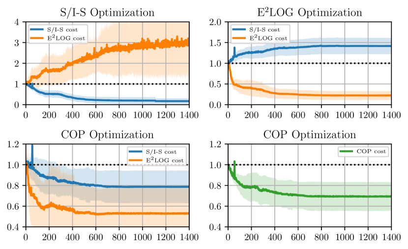
Figure 2: Overview of the cost function evolution during the optimization depicted by averages and $1\sigma$ standard deviations over 20 optimization runs with different initial trajectories. All cost values are normalized with the initial cost prior to the mean calculation. S/I-S cost (blue), E²LOG cost (orange), COP cost (green). All optimizations minimize their respective cost function, therefore, a decrease below 1 (dotted line) is an improvement of the respective objective. Note that the inverse of the E²LOG is used.

IV-A Setup & Evaluation Method

The system model of Sec. II-A, control law of Sec. II-B, and optimization of Sec. III are implemented in Python. All system parameters are based on the quadrotor Hummingbird model of [12]. This previous work shows that it is possible to estimate the thrust force and drag moment coefficients, $k_{f}$ and $k_{m}$. The method of using simulations allows for better repeatability of experiments and avoids the introduction of other artifacts due to uncertainties of the real system.

In this empirical evaluation we look at four types of trajectories: $(i)$ the initial preconditioned trajectory (INIT); $(ii)$ the S/I-S objective optimized one; $(iii)$ the E²LOG objective optimized trajectory; $(iv)$ the new COP objective optimized trajectory. The initial one serves as baseline for all other trajectories. Each trajectory has a duration of $T=20s$, 5 Bézier curve pieces, and a random target way-point $\bm{P}_{T}$ in 3D space with $\left(\mathcal{U}(2,5),\,\mathcal{U}(2,5),\,\mathcal{U}(-0.5,1)\right)$ in meters.

In total, optimizations have been completed for 20 targets, each for the S/I-S, E²LOG, and COP objective. The individual cost functions evolutions, positional mean integral error norms, and estimation uncertainties are evaluated from this set of trajectories. For the positional mean integral error norm evaluation, we chose to randomly perturb the coefficients $k_{f}$ and $k_{m}$ in the ranges of $\pm$1\text{\,}\mathrm{\char 37\relax}\text{/}$$ and $\pm$5\text{\,}\mathrm{\char 37\relax}\text{/}$$ and fulfill 30 closed-loop flights, changing them for every trajectory. Greater perturbations are not considered as such a deviation from the nominal value might hint at problems at the parameter identification/estimation. The estimation uncertainty results are based on 10 runs of each trajectory with different randomly wrong initial guesses ($\pm$30\text{\,}\mathrm{\char 37\relax}\text{/}$$) from ground truth ($k_{f}=$3.375\text{\times}{10}^{-04}\text{\,}\mathrm{N}\mathrm{/}{\mathrm{s}^{-2}}$$ and $k_{m}=$0.016\text{\,}\mathrm{m}\text{/}$$).

IV-B Discussion

IV-B1 Cost Function Behavior

We recorded each objective function’s cost value ($F_{\text{INIT}}$, $F_{\text{\lx@glossaries@gls@link{acronym}{sis}{\leavevmode\mbox{S/I-S}}}}$, $F_{\text{\lx@glossaries@gls@link{acronym}{e2log}{\leavevmode{E${}^{2}$LOG}}}}$, $F_{\text{\lx@glossaries@gls@link{acronym}{cop}{\leavevmode COP}}}$) at all iteration steps during each optimization run to evaluate the behavior of the costs by averaging all runs.

As E²LOG and S/I-S have different orders of magnitudes, a normalization with the initial cost value was performed. In addition, we chose to use the inverted values of E²LOG as they can grow unbound and allows for better comparisons. A decrease ($<$1) means an improvement, while an increase ($>$1) indicates a decline in the performance of the respective objective. As the optimization uses a gradient-free method, the average shows some spikes.

Fig. 2 presents the results of the 20 individual COP runs. The top left plot shows the average and $1\sigma$ standard deviation of the S/I-S-based optimization, Sec. III-C3, with its cost in blue and the E²LOG’s cost in orange. One can see the decrease in the sensitivity cost, meaning that the state and input sensitivities are minimized (as expected). This comes, however, at the expense of the overall quality of observability, indicated by the increase of the inverse E²LOG cost. Therefore, these results seem to indicate that S/I-S and E²LOG can be two conflicting objectives. On the top right are both costs, again blue S/I-S and orange E²LOG, depicted for the quality of observability optimization, Sec. III-C2. As we chose the inverse here, a decrease is equal to an improvement of the E²LOG. Once again, we see the behavior of the left plot reflected in this optimization as well. From those two plots one can infer that if one improves the other might get worse. The two plots at the bottom of Fig. 2 are the results of the optimization runs based on the COP objective, Sec. III-C4. We can see that even distributed weights, as described in Sec. III-C4, can still result in slightly skewed solutions caused by the approximation of the individual utopia and nadir points $F_{i}^{O}$ and $F_{i}^{N}$. The solutions themselves are Pareto optimal, and the straightforward filtering ensures an overall decrease of all considered objectives. This indicates that COP can balance and decrease all objectives.

IV-B2 Control Tracking Error

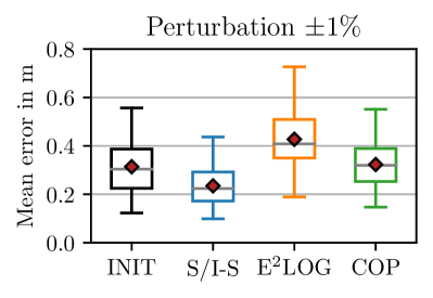
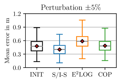
Figure 3: Quartile box plots showing the positional mean integral error norm over the whole trajectory, average over 20 trajectories each with 30 simulated closed-loop flights. The two plots show the influence of different perturbation amplitudes on the parameters $k_{f}$ and $k_{m}$. As expected, the S/I-S optimized one performs best followed by the COP. The E²LOG based trajectories perform worse as they just improve estimation performance. COP as well as S/I-S are most effective with small perturbations, because the sensitivity is evaluated at $\mathbf{p}=\mathbf{p}_{c}$.

The evaluation of the tracking performance of the system with its controller is based on the aforementioned set of trajectories, and is done by considering the positional mean integral error norm of position $\bm{r}(t)$ with respect to the desired position $\bm{r}_{d}(t)$.

The results can be seen in Fig. 3 where we depict the quartile box plots from the statistical data. As mentioned before, each trajectory is flown in simulation 30 times with a changed set of $k_{f}$ and $k_{m}$ for each flight, normally distributed around $\pm$1\text{\,}\mathrm{\char 37\relax}\text{/}$$ and $\pm$5\text{\,}\mathrm{\char 37\relax}\text{/}$$ of their nominal values (which is used to evaluate the various sensitivity quantities).

The quartile boxplots of Fig. 3 show the average tracking performance of each trajectory with different amplitudes of perturbation represented by the mean of the integral of the error norm at each point on the trajectory. The median of the S/I-S optimized trajectory performs the best and the E²LOG one the worst, with COP performing between those two, which confirms Fig. 2 and our expectations. COP can not reach the same performance level as S/I-S because of the balancing in Eq. (12), however, we can improve estimation performance at the same time, Fig. 4. Looking at the evolution of those boxplots, one can see that the farther away $\mathbf{p}$ gets from $\mathbf{p}_{c}$ the less difference is between each objective. This is also expected as the optimization evaluates the trajectories at nominal value. Therefor, one might start with estimation-aware trajectories to get $\mathbf{p}$ as close to $\mathbf{p}_{c}$ and then switches to control-aware ones for improved tracking.

IV-B3 Estimation Error

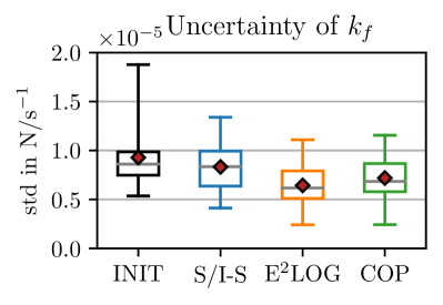
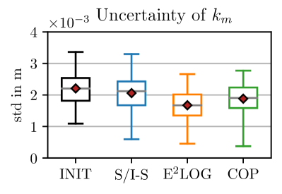
Figure 4: Quartile box plots showing the IEKF’s uncertainty based on the state’s standard deviation at the end of the trajectory, average over 20 trajectories (initial, S/I-S optimized, E²LOG optimized, and E²LOG optimized each) closed-loop flights. Each trajectory is tested with 10 different initial guesses $\pm$30\text{\,}\mathrm{\char 37\relax}\text{/}$$ uniformly distributed around ground truth. (left) is the thrust force coefficient $k_{f}$ and (right) the drag moment coefficient $k_{m}$ depicted. As expected, the initial trajectory has the worst estimation performance and the E²LOG ones are the best with COP generated motions being comparable.

We used the IEKF implementation in Matlab of [12] to evaluate the influence of the trajectories on the estimation of $k_{f}$ and $k_{m}$, which has proven to be good at estimating those parameters. The trajectory optimization is used to generate artificial position sensor and IMU measurements together with rotor speed input for each trajectory. Each of these recordings has been tested using the IEKF with initial guesses of nominal values $k_{f}$ and $k_{m}$ perturbed randomly by $\pm$30\text{\,}\mathrm{\char 37\relax}\text{/}$$ 10 times. Note that both parameters are poorly observable. To visualize the influence, we once again use quartile boxplots for each individual optimization objective. Fig. 4 shows on the left plot the quartile boxplot of $k_{f}$ and on the right for $k_{m}$. The estimation performance is evaluated by the reduction of uncertainty (represented by the standard deviation) at the end of the trajectory at $T$.

One can see that the S/I-S optimized trajectories perform slightly better than the initial ones. This is because we already gain more motion and excitation from the optimization objective. As expected, based on the optimization data, the E²LOG optimized trajectories perform best with the new COP optimized one in between. Note that this is expected, due to the balancing of two objectives we are not able to perform as well as a single objective optimized trajectory. These comparable results were already indicated in Fig. 2. All the presented results support our claim that our proposed COP objective can balance two possibly opposing objectives and maintain good performance.

IV-B4 Computation Times

All trajectory optimizations were done on a PC with an AMD Ryzen 5 3600 CPU (6 cores/12 threads), 16GB Ram, and NVidia RTX 2070 (Super) GPU. Note that one instance of the COP implementation only uses one CPU thread, and therefore, parallelization is possible by starting multiple instances of COP. The duration of each optimization run and each objective were logged. The initial trajectory generation is done in under $120\text{\,}\mathrm{s}\text{/}$. Minimizing the state and input sensitivity metrics ($F_{\Pi}(\bm{a})$ and $F_{\Theta}(\bm{a})$) takes on average $38\text{\,}\min$ and $15\text{\,}\min$, respectively. Improving the observability through the E²LOG ($F_{\text{E${}^{2}$LOG}}(\bm{a})$) needs on average $26\text{\,}\min$. The trajectory optimization with S/I-S ($F_{\text{\lx@glossaries@gls@link{acronym}{sis}{\leavevmode\mbox{S/I-S}}}}(\bm{a})$) finishes in $36\text{\,}\min$ on average. The last objective of the COP approach, minimizing both E²LOG and S/I-S, runs for $27\text{\,}\min$ on average. One complete optimization run needs in total around 2.4 hours which is due to the numerical integration of the complex metrics over the whole trajectory during each iteration of the optimization.

V Conclusion

This paper wanted to answer the question: How to combine Closed-Loop State and Input Sensitivity-based with Observability-aware trajectory planning? Our proposed Control & Observability-aware Planning (COP) framework and its statistical evaluation provide an answer to it.

Intuitively, taking state and input sensitivities into account during the trajectory generation might result in non-informative trajectories for state/parameter estimation. However, informative motions for the estimation process are often difficult to control and likely cause higher tracking errors. Our statistical case study of a 3D quadrotor UAV, focused on system parameters that have a significant impact on the tracking error and are poorly observable (thrust force coefficient $k_{f}$ and drag moment coefficient $k_{m}$), provided insights into the negative correlation between closed-loop state and input sensitivity-based and observability-aware trajectory planning. We were able to show that both objectives work against each other, meaning that while one can improve, the other will get worse. Applying the Augmented Weighted Tchebycheff Method in a multi-step approach to such Multi-objective Optimization Problem (MOOP) allows to balance both in a Single-Objective Optimization Problem (SOOP), improving trajectory tracking and, at the same time, state estimation.

To summarize, we have successfully shown that it is important to consider both objectives as they correlate with each other. The insights and results in this paper give a motivation to go forward with more sophisticated MOOP approaches. Further research should be conducted towards a real-world closed-loop flight using the estimation in the optimization as feedback.

References

- [1] L. Berscheid and T. Kröger, “Jerk-limited Real-time Trajectory Generation with Arbitrary Target States,” in Proceedings of Robotics: Science and Systems XVII (RSS). Robotics: Science and Systems Foundation, July 2021.
- [2] T. Löw, T. Bandyopadhyay, J. Williams, and P. V. Borges, “PROMPT: Probabilistic Motion Primitives based Trajectory Planning,” in Proceedings of Robotics: Science and Systems XVII (RSS). Robotics: Science and Systems Foundation, July 2021.
- [3] D. Mellinger and V. Kumar, “Minimum Snap Trajectory Generation and Control for Quadrotors,” in 2011 IEEE International Conference on Robotics and Automation (ICRA), May 2011, pp. 2520–2525.
- [4] F. Morbidi, R. Cano, and D. Lara, “Minimum-Energy Path Generation for a Quadrotor UAV,” in 2016 IEEE International Conference on Robotics and Automation (ICRA), May 2016, pp. 1492–1498.
- [5] H. Chen, P. Lu, and C. Xiao, “Dynamic Obstacle Avoidance for UAVs Using a Fast Trajectory Planning Approach,” in 2019 IEEE International Conference on Robotics and Biomimetics (ROBIO), December 2019, pp. 1459–1464.
- [6] B. Shi, Y. Zhang, L. Mu, J. Huang, J. Xin, Y. Yi, S. Jiao, G. Xie, and H. Liu, “UAV Trajectory Generation Based on Integration of RRT and Minimum Snap Algorithms,” in 2020 Chinese Automation Congress (CAC), November 2020, pp. 4227–4232.
- [7] H. Oleynikova, M. Burri, Z. Taylor, J. Nieto, R. Siegwart, and E. Galceran, “Continuous-Time Trajectory Optimization for Online UAV Replanning,” in 2016 IEEE/RSJ International Conference on Intelligent Robots and Systems (IROS), October 2016, pp. 5332–5339.
- [8] S. Candido and S. Hutchinson, “Minimum Uncertainty Robot Path Planning using a POMDP Approach,” in 2010 IEEE/RSJ International Conference on Intelligent Robots and Systems (IROS), December 2010, pp. 1408–1413.
- [9] Y. Liu, H. Wang, J. Fan, J. Wu, and T. Wu, “Control-oriented UAV highly feasible trajectory planning: A deep learning method,” Aerospace Science and Technology, vol. 110, p. 106435, March 2021.
- [10] A. Schperberg, S. Tsuei, S. Soatto, and D. Hong, “SABER: Data-Driven Motion Planner for Autonomously Navigating Heterogeneous Robots,” IEEE Robotics and Automation Letters (RA-L), pp. 1–1, 2021.
- [11] C. Xi and X. Liu, “Unmanned Aerial Vehicle Trajectory Planning via Staged Reinforcement Learning,” in 2020 International Conference on Unmanned Aircraft Systems (ICUAS), 2020, pp. 246–255.
- [12] C. Böhm, M. Scheiber, and S. Weiss, “Filter-Based Online System-Parameter Estimation for Multicopter UAVs,” in Proceedings of Robotics: Science and Systems XVII. Robotics: Science and Systems Foundation, July 2021.
- [13] K. Hausman, J. Preiss, G. S. Sukhatme, and S. Weiss, “Observability-Aware Trajectory Optimization for Self-Calibration With Application to UAVs,” IEEE Robotics and Automation Letters (RA-L), vol. 2, no. 3, pp. 1770–1777, July 2017.
- [14] J. A. Preiss, K. Hausman, G. S. Sukhatme, and S. Weiss, “Simultaneous self-calibration and navigation using trajectory optimization,” The International Journal of Robotics Research (IJRR), vol. 37, no. 13-14, pp. 1573–1594, August 2018.
- [15] C. Böhm, G. Li, G. Loianno, and S. Weiss, “Observability-Aware Trajectories for Geometric and Inertial Self-Calibration,” in Power On and Go Robots 2020, RSS’20, (Virtual) Workshop, July 2020.
- [16] A. D. Wilson, J. A. Schultz, and T. D. Murphey, “Trajectory Optimization for Well-Conditioned Parameter Estimation,” IEEE Transactions on Automation Science and Engineering (T-ASE), vol. 12, no. 1, pp. 28–36, May 2015.
- [17] S. Ponda, R. Kolacinski, and E. Frazzoli, “Trajectory Optimization for Target Localization Using Small Unmanned Aerial Vehicles,” in AIAA Guidance, Navigation, and Control Conference, August 2009, p. 6015.
- [18] J. van den Berg, P. Abbeel, and K. Goldberg, “LQG-MP: Optimized Path Planning for Robots with Motion Uncertainty and Imperfect State Information,” The International Journal of Robotics Research (IJRR), vol. 30, no. 7, pp. 895–913, June 2011.
- [19] A. Ansari and T. Murphey, “Minimum Sensitivity Control for Planning with Parametric and Hybrid Uncertainty,” The International Journal of Robotics Research (IJRR), vol. 35, no. 7, pp. 823–839, October 2016.
- [20] T. Lee, M. Leok, and N. H. McClamroch, “Geometric Tracking Control of a Quadrotor UAV on SE(3),” in 49th IEEE Conference on Decision and Control (CDC), December 2010, pp. 5420–5425.
- [21] M. Kamel, T. Stastny, K. Alexis, and R. Siegwart, “Model Predictive Control for Trajectory Tracking of Unmanned Aerial Vehicles Using Robot Operating System,” in Robot Operating System (ROS): The Complete Reference (Volume 2). Springer International Publishing, 2017, pp. 3–39.
- [22] P. Brault, Q. Delamare, and P. Robuffo Giordano, “Robust Trajectory Planning with Parametric Uncertainties,” in 2021 IEEE International Conference on Robotics and Automation (ICRA), June 2021.
- [23] P. Robuffo Giordano, Q. Delamare, and A. Franchi, “Trajectory Generation for Minimum Closed-Loop State Sensitivity,” in 2018 IEEE International Conference on Robotics and Automation (ICRA), June 2018, pp. 286–293.
- [24] R. Mahony, V. Kumar, and P. Corke, “Multirotor Aerial Vehicles: Modeling, Estimation, and Control of Quadrotor,” IEEE Robotics Automation Magazine (RAM), vol. 19, no. 3, pp. 20–32, Sep. 2012.
- [25] P. Robuffo Giordano, Q. Delamare, and A. Franchi, “Trajectory Generation for Minimum Closed-Loop State Sensitivity,” in 2018 IEEE International Conference on Robotics and Automation (ICRA), May 2018, pp. 286–293.
- [26] S. Weiss, M. W. Achtelik, M. Chli, and R. Siegwart, “Versatile Distributed Pose Estimation and Sensor Self-Calibration for an Autonomous MAV,” in 2012 IEEE International Conference on Robotics and Automation (ICRA), May 2012, pp. 31–38.
- [27] K. Hausman, S. Weiss, R. Brockers, L. Matthies, and G. S. Sukhatme, “Self-Calibrating Multi-Sensor Fusion with Probabilistic Measurement Validation for Seamless Sensor Switching on a UAV,” in 2016 IEEE International Conference on Robotics and Automation (ICRA), May 2016, pp. 4289–4296.
- [28] R. Hermann and A. Krener, “Nonlinear controllability and observability,” IEEE Transactions on Automatic Control (TAC), vol. 22, no. 5, pp. 728–740, October 1977.
- [29] A. J. Krener and K. Ide, “Measures of Unobservability,” in Proceedings of the 48h IEEE Conference on Decision and Control (CDC), Dec 2009, pp. 6401–6406.
- [30] R. E. Steuer and E.-U. Choo, “An interactive weighted Tchebycheff procedure for multiple objective programming,” Mathematical programming, vol. 26, no. 3, pp. 326–344, October 1983.
- [31] A. P. Wierzbicki, “Multiple Criteria Games - Theory and Applications,” Journal of Systems Engineering and Electronics, vol. 6, no. 2, pp. 65–81, June 1995.
- [32] R. T. Marler and J. S. Arora, “Survey of multi-objective optimization methods for engineering,” Structural and multidisciplinary optimization, vol. 26, no. 6, pp. 369–395, March 2004.
- [33] K. Dächert, J. Gorski, and K. Klamroth, “An Adaptive Augmented Weighted Tchebycheff Method to solve Discrete, Integer-valued Bicriteria Optimization Problems,” University of Wuppertal, Tech. Rep. BUWAMNA-OPAP 10/06, April 2010.
- [34] M. T. Emmerich and A. H. Deutz, “A tutorial on multiobjective optimization: fundamentals and evolutionary methods,” Natural computing, vol. 17, no. 3, pp. 585–609, May 2018.
- [35] T. Holzmann and J. C. Smith, “Solving discrete multi-objective optimization problems using modified augmented weighted Tchebychev scalarizations,” European Journal of Operational Research, vol. 271, no. 2, pp. 436–449, December 2018.