Hodge allocation for cooperative rewards:
a generalization of Shapley’s cooperative value allocation theory via Hodge theory on graphs

Abstract.

Lloyd Shapley’s cooperative value allocation theory is a central concept in game theory that is widely used in various fields to allocate resources, assess individual contributions, and determine fairness. The Shapley value formula and his four axioms that characterize it form the foundation of the theory.

Shapley value can be assigned only when all cooperative game players are assumed to eventually form the grand coalition. The purpose of this paper is to extend Shapley’s theory to cover value allocation at every partial coalition state.

To achieve this, we first extend Shapley axioms into a new set of five axioms that can characterize value allocation at every partial coalition state, where the allocation at the grand coalition coincides with the Shapley value. Second, we present a stochastic path integral formula, where each path now represents a general coalition process. This can be viewed as an extension of the Shapley formula. We apply these concepts to provide a dynamic interpretation and extension of the value allocation schemes of Shapley, Nash, Kohlberg and Neyman.

This generalization is made possible by taking into account Hodge calculus, stochastic processes, and path integration of edge flows on graphs. We recognize that such generalization is not limited to the coalition game graph. As a result, we define Hodge allocation, a general allocation scheme that can be applied to any cooperative multigraph and yield allocation values at any cooperative stage.

Keywords: Cooperative game, Shapley value, Shapley axioms, Shapley formula, Hodge allocation, Poisson’s equation, $f$-Shapley value, Markov chain, edge flow, stochastic path integral, multigraph, Nash solution, Kohlberg-Neyman’s value

MSC2020 Classification: 60J20, 60H30, 68R01, 05C57, 91A12

1. Introduction

Lloyd Shapley’s value allocation theory for cooperative games has been one of the most central concepts in game theory. Shapley value is widely used in many fields, including economics, finance, and machine learning, to allocate resources, assess individual agent contributions, and determine the fairness of payouts. Among many excellent treatises on Shapley value, we refer to a recent treatise by Algaba et al. [1], in which various authors discuss modern applications of the Shapley value to various game-theoretic and operations-research problems including genetics, social choice and social network, finance, politics, tax games, telecommunication and energy transmission networks, queueing problems, group decision making, spanning trees, and even aircraft landing fees problem. Recently, researchers have begun to use the Shapley value in machine learning [27]. This shows that Shapley’s cooperative value allocation theory is still an active research topic applied to a variety of situations, and continues to inspire many researchers in a variety of fields.

Shapley value has two very interesting aspects: Shapley’s famous value allocation formula and his four axioms that characterize it. The Shapley axioms are intriguing and significant because they provide a set of fairness criteria for determining the value of a cooperative game and individual player contributions. These axioms ensure that the value distribution in a game is fair, transparent, and consistent with our intuitive understanding of what is fair. Because it satisfies these axioms, the Shapley value is regarded as a unique and compelling solution to the problem of allocating the value of a cooperative game. The Shapley formula is also significant because it provides a mathematical method for calculating the value of a cooperative game and individual player contribution. The formula determines each player’s marginal contribution to the total value of the game by permuting all possible coalitions of players. The Shapley formula has several desirable properties inherited from the Shapley axioms, which make it a popular method for evaluating individual player performance and allocating the value of a cooperative game.

It is worth noting that Shapley value can be assigned only when all players are assumed to eventually form the grand coalition, and Shapley axioms and formula then determine the fair allocation. In other words, Shapley value does not address how to properly assess individual player contribution and allocate the value of a cooperative game when the players form any non-grand, but partial coalition state.

The purpose of this paper is to complete the missing piece. More specifically, we will provide generalizations of Shapley axioms and the Shapley formula, so that the new theory can now characterize a value allocation at every partial coalition state, where the allocation at the grand coalition coincides with the Shapley value.

The inclusion of all partial coalitions as potential target states in the cooperative value allocation theory is significant because, in practice, coalition formation often results in a partial coalition of a group of people rather than all of the people. The Shapley formula assumes that coalition formation will continue to grow, with each step resulting in a new player joining an existing coalition until all players form the grand coalition. To adequately describe the progress of any partial coalition, we generalize the coalition process so that players can not only join but also leave an existing coalition until the destined coalition is formed. This is significant as well because it provides a more general and realistic description of coalition processes. Indeed, the generalized coalition process inspired our new fifth axiom and value allocation formula, which can be viewed as a generalization of the Shapley formula.

As we build the new allocation theory using Hodge calculus, stochastic processes, and path integration on graphs, it gradually becomes clear that such generalization should not be limited to the coalition game graph setting. As a result, we are led to define Hodge allocation, a general allocation scheme that can be applied to any cooperative multigraph and yield allocation values at any cooperative stage. Finally, we demonstrate how the Hodge allocation can be calculated effectively on any multigraph if the underlying cooperative process satisfies a natural property.

This paper is organized as follows. In Section 2, we review Shapley’s cooperative value allocation theory. In Section 3, we review Stern and Tettenhorst’s interpretation of the Shapley value in terms of combinatorial Poisson’s equation on coalition game graph. In Section 4, we present our extension of the Shapley axioms and value allocation formula to address allocation schemes for all partial coalitions and their axiomatic characterization, as well as their dynamic interpretation via the random coalition process. In Section 5, we generalize the Shapley value by relaxing the null player axiom and employing arbitrary edge flows as players’ marginal value. In Section 6, we show how our findings can be applied to extend Nash’s and Kohlberg–Neyman’s value allocation scheme for the cooperative strategic games. In Sections 7 and 8, Hodge allocation is introduced as our most general allocation scheme, which can be applied to any cooperative multigraph and yield allocation values at any cooperative stage. Finally, Section 9 presents proofs of the results.

2. Review of Shapley axioms and the Shapley formula

Let us review the now-classic Shapley’s value allocation theory [28, 29, 30], which continues to inspire many researchers in various fields. We refer to Ray [23] for a comprehensive overview of game theory and its applications to coalition formation.

To begin, let $[N]:=\{1,2,...,N\}$ represent the players of the coalition games

$${\cal G}_{N}=\{v:2^{[N]}\to{\mathbb{R}}\ |\ v(\emptyset)=0\}.$$

Thus, a coalition game $v$ is simply a (value) function on the subsets of $[N]$, where each $S\subseteq[N]$ represents a coalition of players in $S$, and $v(S)$ represents the value assigned to the coalition $S$, with the null coalition $\emptyset$ receiving zero value. Shapley considered the question of how to split the grand coalition value $v([N])$ among the players for a given game $v\in{\cal G}_{N}$. It is determined uniquely by the following result.

Theorem 2.1 (Shapley [28]).

There exists a unique allocation $v\in{\cal G}_{N}\mapsto\bigl{(}\phi_{i}(v)\bigr{)}_{i\in[N]}$ satisfying the following conditions:

$\cdot$ efficiency: $\sum_{i\in[N]}\phi_{i}(v)=v([N])$.

$\cdot$ symmetry: $v\bigl{(}S\cup\{i\}\bigr{)}=v\bigl{(}S\cup\{j\}\bigr{)}$ for all $S\subseteq[N]\setminus\{i,j\}$ yields $\phi_{i}(v)=\phi_{j}(v)$.

$\cdot$ null-player: $v\bigl{(}S\cup\{i\}\bigr{)}-v(S)=0$ for all $S\subseteq[N]\setminus\{i\}$ yields $\phi_{i}(v)=0$.

$\cdot$ linearity: $\phi_{i}(\alpha v+\alpha^{\prime}v^{\prime})=\alpha\phi_{i}(v)+\alpha^{\prime}\phi_{i}(v^{\prime})$ for all $\alpha,\alpha^{\prime}\in\mathbb{R}$ and $v,v^{\prime}\in{\cal G}_{N}$.

Moreover, this allocation is given by the following explicit formula:

(2.1) $$\phi_{i}(v)=\sum_{S\subseteq[N]\setminus\{i\}}\frac{\lvert S\rvert!\bigl{(}N-1-\lvert S\rvert\bigr{)}!}{N!}\Bigl{(}v\bigl{(}S\cup\{i\}\bigr{)}-v(S)\Bigr{)}.$$

The four conditions listed above are commonly referred to as the Shapley axioms. According to [31], [efficiency] means that the value obtained by the grand coalition is fully distributed among the players, [symmetry] means that equivalent players receive equal amounts, [null-player] means that a player who contributes no marginal value to any coalition receives nothing, and [linearity] means that the allocation is linear in game values. And (2.1) is referred to as the Shapley formula.

(2.1) can be rewritten also according to [31]: Suppose the players form the grand coalition by joining, one-at-a-time, in the order defined by a permutation $\sigma$ of $[N]$. That is, player $i$ joins immediately after the coalition $S^{\sigma}_{i}=\bigl{\{}j\in[N]:\sigma(j)<\sigma(i)\bigr{\}}$ has formed, contributing marginal value $v\bigl{(}S^{\sigma}_{i}\cup\{i\}\bigr{)}-v(S^{\sigma}_{i})$. Then $\phi_{i}(v)$ is the average marginal value contributed by player $i$ over all $N!$ permutations $\sigma$, i.e.,

(2.2) $$\phi_{i}(v)=\frac{1}{N!}\sum_{\sigma}\Bigl{(}v\bigl{(}S^{\sigma}_{i}\cup\{i\}\bigr{)}-v(S^{\sigma}_{i})\Bigr{)}.$$

The well-known glove game below explains the formula (2.2) in a simple context.

Example 2.2 (Glove game).

Let $N=3$. Suppose player $1$ has a left-hand glove, while players $2$ and $3$ each have a right-hand glove. A pair of gloves has value $1$, while unpaired gloves have no value, i.e., $v(S)=1$ if $S\subseteq[N]$ contains player $1$ and at least one of players $2$ or $3$, and $v(S)=0$ otherwise. The Shapley values are given by:

$$\phi_{1}(v)=\frac{2}{3},\qquad\phi_{2}(v)=\phi_{3}(v)=\frac{1}{6}.$$

This is easily seen from (2.2): player $1$ contributes marginal value $0$ when joining the coalition first (2 of 6 permutations) and marginal value $1$ otherwise (4 of 6 permutations), so $\phi_{1}(v)=\frac{2}{3}$. Efficiency and symmetry yield $\phi_{2}(v)=\phi_{3}(v)=\frac{1}{6}$.

Since its inception in 1953, the theory have influenced many researchers and have been followed by research works such as Chun [3], Deng and Papadimitriou [4], Derks and Haller [5], Faigle and Kern [6], Gul [7], Hsiao and Raghavan [8], Kalai and Samet [10], Kohlberg and Neyman [11, 12], Kultti and Salonen [13], Maniquet [17], Myerson [18, 19, 20], Nash [21], Pérez-Castrillo and Wettstein [22], Roth [24, 25], Rozemberczki et al. [27], Young [32], to only name a few. We will focus on Stern and Tettenhorst [31], who recently reexamined Shapley’s results via combinatorial Hodge theory on graphs. The following section, which will serve as our starting point, will cover the basic definition of differential calculus on graphs.

3. Stern and Tettenhorst’s interpretation of Shapley value

Recently, the combinatorial Hodge decomposition has been applied to game theory in a variety of contexts, e.g., noncooperative games (Candogan et al. [2]), cooperative games (Stern and Tettenhorst [31]), and ranking of social preferences (Jiang et al. [9]). In order to provide a new interpretation of the Shapley value, [31] focused on the hypercube graph, or coalition game graph $G=({\cal V},{\cal E})$, where ${\cal V}$ denotes the set of nodes and ${\cal E}$ the set of edges. This graph is defined by

(3.1) $${\cal V}:=2^{[N]},\ \ {\cal E}:=\bigl{\{}\bigl{(}S,S\cup\{i\}\bigr{)}\in{\cal V}\times{\cal V}\ |\ S\subseteq[N]\setminus\{i\},\ i\in[N]\bigr{\}}.$$

Notice that each coalition $S\subseteq[N]$ can correspond to a vertex of the unit hypercube in ${\mathbb{R}}^{N}$. We assume that each edge is oriented in the direction of the inclusion $S\hookrightarrow S\cup\{i\}$. We also define the set of reverse (or negatively-oriented) edges

(3.2) $${\cal E}_{-}:=\bigl{\{}\bigl{(}S\cup\{i\},S\bigr{)}\in{\cal V}\times{\cal V}\ |\ S\subseteq[N]\setminus\{i\},\ i\in[N]\bigr{\}}.$$

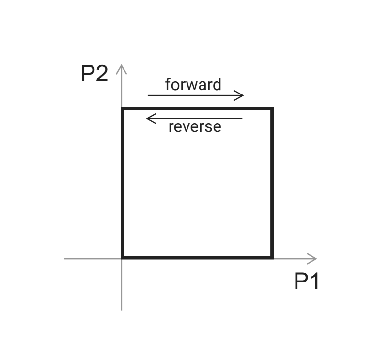
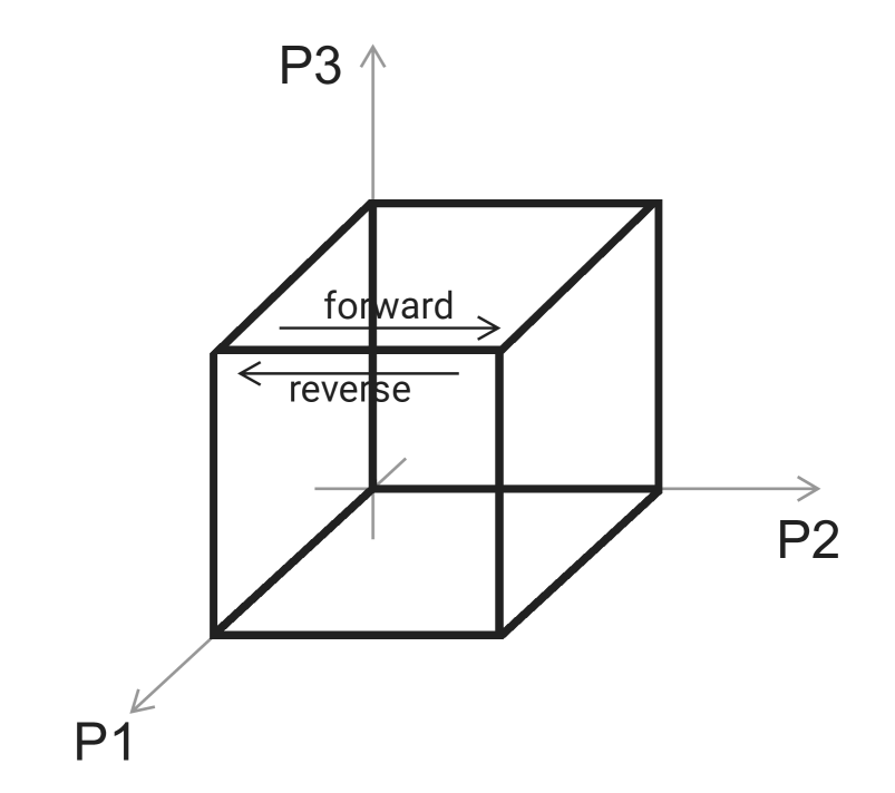
Figure 1. Coalition game graph for $N=2$ and $3$. Each vertex of the cube corresponds to a coalition. The vertex $(1,0,1)$, for example, corresponds to the coalition $\{1,3\}$, $(0,1,1)$ to $\{2,3\}$, and so on.

The edges in ${\cal E}$ are then called forward or positively-oriented edges. Let $\overline{\cal E}:={\cal E}\cup{\cal E}_{-}$.

The Shapley formula (2.1) clearly inspires us to consider the gradient, a linear operator that describes the marginal value $v\bigl{(}S\cup\{i\}\bigr{)}-v(S)$ for a given player $i$ and game $v$. To introduce the gradient and its adjoint, the divergence, we must first introduce the inner product space of functions as follows. We denote by $\ell^{2}({\cal V})$ the space of functions ${\cal V}\rightarrow\mathbb{R}$ equipped with the standard inner product

(3.3) $$\langle u,v\rangle\coloneqq\sum_{S\in{\cal V}}u(S)v(S).$$

We may recall that a coalition game $v$ is simply an element in $\ell^{2}({\cal V})$ with the initial condition $v(\emptyset)=0$. We then denote by $\ell^{2}({\cal E})$ the space of functions $\overline{\cal E}\rightarrow\mathbb{R}$ equipped with the inner product

(3.4) $$\langle f,g\rangle\coloneqq\sum_{(S,S\cup\{i\})\in{\cal E}}f\bigl{(}S,S\cup\{i\}\bigr{)}\,g\bigl{(}S,S\cup\{i\}\bigr{)}$$

satisfying the alternating condition

(3.5) $$f\bigl{(}S\cup\{i\},S\bigr{)}\coloneqq-f\bigl{(}S,S\cup\{i\}\bigr{)},$$

which is a crucial assumption in Hodge theory. Thus every $f\in\ell^{2}({\cal E})$ (also known as an edge flow) is defined on $\overline{\cal E}={\cal E}\cup{\cal E}_{-}$, but note that the inner product is only taken on the forward edges.

We can now endow $G$ with a Hodge differential structure [14]. For $v\in\ell^{2}({\cal V})$, we naturally define a linear operator $\mathrm{d}\colon\ell^{2}({\cal V})\rightarrow\ell^{2}({\cal E})$, the gradient, by

(3.6) $$\mathrm{d}v\bigl{(}S,S\cup\{i\}\bigr{)}\coloneqq v(S\cup\{i\})-v(S).$$

Note $\mathrm{d}v\in\ell^{2}({\cal E})$. The adjoint operator $\mathrm{d}^{\ast}$, called (negative) divergence, is given by

(3.7) $$\mathrm{d}^{*}f(S)=\sum_{T\sim S}f(T,S)$$

where $T\sim S$ means that $S$ and $T$ are adjacent on the graph. $\mathrm{d}$ and $\mathrm{d}^{\ast}$ then satisfy the defining relation

(3.8) $$\langle\mathrm{d}v,f\rangle=\langle v,\mathrm{d}^{\ast}f\rangle\ \text{ for all }\,v\in\ell^{2}({\cal V}),\,f\in\ell^{2}({\cal E}).$$

The graph Laplacian is now defined by the operator $\mathrm{d}^{\ast}\mathrm{d}:\ell^{2}({\cal V})\to\ell^{2}({\cal V})$. Finally, for each $i\in[N]$, let $\mathrm{d}_{i}\colon\ell^{2}({\cal V})\rightarrow\ell^{2}({\cal E})$ denote the partial differential operator

(3.9) $$\mathrm{d}_{i}v\bigl{(}S,S\cup\{j\}\bigr{)}:=\begin{cases}\mathrm{d}v\bigl{(}S,S\cup\{i\}\bigr{)}&\text{if }\ j=i,\\ 0&\text{if }\ j\neq i.\end{cases}$$

$\mathrm{d}_{i}v\in\ell^{2}({\cal E})$ encodes the marginal value contributed by player $i$ to the game $v$. Given $v\in{\cal G}_{N}$, Stern and Tettenhorst [31] defined the component game $v_{i}$ for each $i\in[N]$ as the unique solution in ${\cal G}_{N}$ to the following form of Poisson’s equation

(3.10) $$\mathrm{d}^{\ast}\mathrm{d}v_{i}=\mathrm{d}^{\ast}\mathrm{d}_{i}v.$$

Note that $\mathrm{d}^{\ast}\mathrm{d}u=0$ implies $\mathrm{d}u=0$, which implies that $u$ is constant if $G$ is a connected graph. Due to the initial condition $v_{i}(\emptyset)=0$, this results in the uniqueness of the component games $(v_{i})_{i\in[N]}$.

Now [31] showed that the component game $v_{i}$ solving (3.10) in fact satisfies

(3.11) $$v_{i}([N])=\phi_{i}(v)\ \text{ for every }\ i\in[N],$$

obtaining a new characterization of the Shapley value as the players’ component game value at the grand coalition. We may recall that the Shapley formula reveals that the Shapley value is entirely determined by the player $i$’s marginal value, i.e., $\mathrm{d}_{i}v$, which may inspire them to study the Poisson’s equation of the form (3.10).

However, notice each component game $v_{i}$ is not just defined at the grand coalition state $[N]$ but at any state $S\subseteq[N]$. This leads us to ask the following question.

Question: What is the economic significance of the value $v_{i}(S)$, when $S\subsetneq[N]$?

The explicit calculations that follow make this question more interesting. Let $\delta_{[N]}\in{\cal G}_{N}$ denote the pure bargaining game, given by $\delta_{[N]}([N])=1$ and $\delta_{[N]}(S)=0\,\text{ if }\,S\subsetneq[N].$ One can calculate the component games $(v_{i})_{i}$ for the pure bargaining game $\delta_{[N]}$ using the formulas in [31]. For example, for $N=2,3$, we have

$N=2$	$\{1\}$	$\{2\}$	$\{1,2\}$
$v_{1}$	$\frac{1}{4}$	-$\frac{1}{4}$	$\frac{1}{2}$
$v_{2}$	-$\frac{1}{4}$	$\frac{1}{4}$	$\frac{1}{2}$

$N=3$	$\{1\}$	$\{2\}$	$\{3\}$	$\{1,2\}$	$\{1,3\}$	$\{2,3\}$	$\{1,2,3\}$
$v_{1}$	$\frac{1}{12}$	-$\frac{1}{24}$	-$\frac{1}{24}$	$\frac{1}{8}$	$\frac{1}{8}$	-$\frac{1}{4}$	$\frac{1}{3}$
$v_{2}$	-$\frac{1}{24}$	$\frac{1}{12}$	-$\frac{1}{24}$	$\frac{1}{8}$	-$\frac{1}{4}$	$\frac{1}{8}$	$\frac{1}{3}$
$v_{3}$	-$\frac{1}{24}$	-$\frac{1}{24}$	$\frac{1}{12}$	-$\frac{1}{4}$	$\frac{1}{8}$	$\frac{1}{8}$	$\frac{1}{3}$

Even for such a simple game $\delta_{[N]}$, the formulas in [31, Theorem 3.13] become increasingly complicated as $N$ grows, and we hardly find any pattern in the values. However, we can observe that $v_{i}$ can take negative values even if $v$ is nonnegative.

We will now present an extension of the Shapley axioms, which can now characterize the component game values at each coalition state. We will also discuss how considering a natural random coalition process will inspire the fifth axiom.

4. Generalized Shapley axioms and its dynamic interpretation

Stern and Tettenhorst’s new characterization of the Shapley value (3.11) prompts us to ask the following question: If the Shapley axioms can characterize the Shapley value $v_{i}([N])$, are there conditions that can also characterize the values $v_{i}(S)$ for all states $S$? In other words, are there conditions that can characterize the solutions to the Poisson equation $\mathrm{d}^{\ast}\mathrm{d}v_{i}=\mathrm{d}^{\ast}\mathrm{d}_{i}v$ for any $v\in{\cal G}_{N}$? And, if they do exist, will they have corresponding economic interpretation as the Shapley axioms?

This question is addressed in our first main result, which provides an axiomatic description of the values $v_{i}(S)$ for every $i\in[N]$ and $S\subseteq[N]$. In other words, we will look for conditions that completely determine the solutions to (3.10).

For this, let ${\cal G}=\bigcup_{N\in{\mathbb{N}}}{\cal G}_{N}$. For $i,j\in[N]$ and $S\subseteq[N]$, we define $S^{ij}\subseteq[N]$ by

$$S^{ij}=\begin{cases}S&\text{if }\ S\subseteq[N]\setminus\{i,j\}\,\text{ or }\,\{i,j\}\subseteq S,\\ S\cup\{i\}\setminus\{j\}&\text{if }\ i\notin S\,\text{ and }\,j\in S,\\ S\cup\{j\}\setminus\{i\}&\text{if }\ j\notin S\,\text{ and }\,i\in S.\end{cases}$$

Given $v\in{\cal G}_{N}$ and $i,j\in[N]$, we define $v^{ij}\in{\cal G}_{N}$ by $v^{ij}(S)=v(S^{ij})$. Intuitively, the contributions of the players $i,j$ in the game $v$ are interchanged in the game $v^{ij}$.

Of course, a coalition game can be considered on any finite set of players $M$ through a bijection $M\hookrightarrow[|M|]$. In this sense, we define $v_{-i}$ to be the restricted game of $v$ on the set of players $[N]\setminus\{i\}$, i.e., $v_{-i}(S)=v(S)$ for all $S\subseteq[N]\setminus\{i\}$. We can now describe our axioms and how they characterize the component games.

Theorem 4.1.

There exists a unique allocation map $v\in{\cal G}\mapsto\bigl{(}\Phi_{i}[v]\bigr{)}_{i\in{\mathbb{N}}}$ satisfying $\Phi_{i}[v]\in{\cal G}_{N}$ with $\Phi_{i}[v]\equiv 0$ for $i>N$ if $v\in{\cal G}_{N}$, and also the following conditions:

A1(efficiency): $v=\sum_{i\in{\mathbb{N}}}\Phi_{i}[v]$.

A2(symmetry): $\Phi_{i}[v^{ij}](S^{ij})=\Phi_{j}[v](S)$ for all $v\in{\cal G}_{N}$, $i,j\in[N]$ and $S\subseteq[N]$.

A3(null-player): If $v\in{\cal G}_{N}$ and $\mathrm{d}_{i}v=0$ for some $i\in[N]$, then $\Phi_{i}[v]\equiv 0$, and

$$\Phi_{j}[v](S\cup\{i\})=\Phi_{j}[v](S)=\Phi_{j}[v_{-i}](S)\ \text{ for all }\ j\in[N]\setminus\{i\},\,S\subseteq[N]\setminus\{i\}.$$

A4(linearity): For any $v,v^{\prime}\in{\cal G}_{N}$ and $\alpha,\alpha^{\prime}\in{\mathbb{R}}$, $\Phi_{i}[\alpha v+\alpha^{\prime}v^{\prime}]=\alpha\Phi_{i}[v]+\alpha^{\prime}\Phi_{i}[v^{\prime}]$.

A5(reflection): For any $v\in{\cal G}_{N}$ and $S\subseteq[N]\setminus\{i,j\}$ with $i\neq j$, it holds

$$\Phi_{i}[v](S\cup\{i,j\})-\Phi_{i}[v](S\cup\{i\})=-\big{(}\Phi_{i}[v](S\cup\{j\})-\Phi_{i}[v](S)\big{)}.$$

Furthermore, the solution $v_{i}\in{\cal G}_{N}$ to (3.10) satisfy A1–A5 with the identification $\Phi_{i}[v]=v_{i}$. In other words, A1–A5 characterizes the solutions $\{v_{i}\}_{i\in[N]}$ to (3.10).

In light of this characterization of the component values, our conditions A1–A5 can be viewed as a completion of Shapley’s original four axioms. Among these, first of all, A1 and A4 are natural analogues of the corresponding Shapley axioms.

The condition in A2 is the same as if the players $i,j$ switched labels. We can interpret as follows: if the contributions of $i,j$ are interchanged, so are their payoffs.

A3 states that if $\mathrm{d}_{i}v=0$, everything is the same as if $i$ is not present. In other words, if player $i$ contributes no marginal value, the reward of the rest is independent of the null player $i$’s participation, thus the player $i$ receives nothing by efficiency. So $\Phi_{i}[v]\equiv 0$ is a consequence rather than a part of the axioms.

We see that A1–A4 are a natural extension of the Shapley axioms now to deal with different numbers of players $N$ and coalitions $S$, as well as their symmetric counterpart $S^{ij}$. In particular, A1–A4 will determine the Shapley value $v_{i}([N])$. However, A1–A4 appear to be insufficient to fully determine $v_{i}(S)$ for all coalitions $S\subseteq[N]$, and our observation is that the reflection condition A5 appears to be the key to complement A1–A4, on which we will now elaborate.

Recall that in the Shapley formula (2.1), the coalition formation is supposed to be only increasing, with each step resulting in a player joining a given coalition. In contrast, let us consider a random coalition process, described by the canonical Markov chain $(X^{S}_{n})_{n\in{\mathbb{N}}_{0}}$ on the state space ${\cal V}$ in (3.1) with initial state $X_{0}=S\in{\cal V}$, equipped with the transition probability $p_{S,T}$ from a state $S$ to $T$ given by

(4.1) $$p_{S,T}=1/N\ \text{ if }\ T\sim S,\quad p_{S,T}=0\ \text{ if }\ T\not\sim S.$$

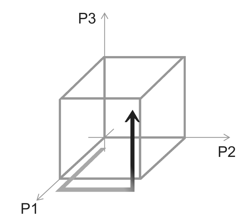
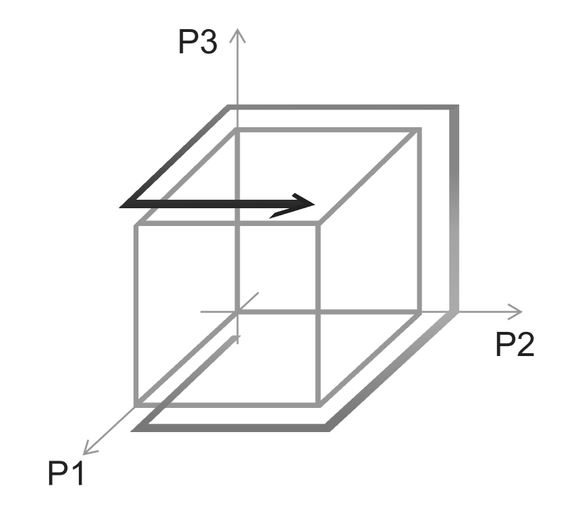
Figure 2. Examples of Shapley’s coalition path and our general coalition path. The path in this example has no loops, but in general, our coalition path is allowed to have an arbitrary number of loops.

In other words, the process is an unbiased random walk on the hypercube graph, describing the canonical coalition progression in which every player has an equal chance of joining or leaving the current coalition state at any time.

Let $(\Omega,{\cal F},{\cal P})$ denote the underlying probability space for formality. For each $S,T\in{\cal V}$ and a sample coalition path $\omega\in\Omega$, let $\tau_{T}=\tau_{T}(\omega)\in{\mathbb{N}}$ denote the first (random) time the coalition process $\big{(}X^{S}_{n}(\omega)\big{)}_{n}$ visits $T$. We assume $\tau\geq 1$, i.e., if the coalition starts at $T$, then $\tau_{T}$ denotes the process’s first return time to $T$.

Now given a coalition game $v\in{\cal G}_{N}$, the total contribution of player $i$ along the sample path $\omega$ traveling from $S$ to $T$ can be calculated as

(4.2) $${\cal I}_{i}^{S}(T)={\cal I}_{i}^{S}(T)(\omega):=\sum_{n=1}^{\tau_{T}(\omega)}\mathrm{d}_{i}v\big{(}X^{S}_{n-1}(\omega),X^{S}_{n}(\omega)\big{)}.$$

Given that the coalition has progressed from $S$ to $T$ along the path $\omega$, (4.2) represents player $i$’s total contribution throughout the progression. Thus, the value function given by the following stochastic path integral

(4.3) $$V_{i}^{S}(T):=\int_{\Omega}{\cal I}_{i}^{S}(T)(\omega)d{\cal P}(\omega)={\mathbb{E}}[{\cal I}_{i}^{S}(T)]$$

represents player $i$’s expected total contribution if the state advances from $S$ to $T$.

If the initial state is $\emptyset$, we omit the upper script and write $(X_{n})_{n\in{\mathbb{N}}_{0}}$, ${\cal I}_{i}(\cdot)$ and $V_{i}(\cdot)$. Theorem 4.1 discussed the component games $(v_{i})_{i}$, whereas the value function $(V_{i})_{i}$ is defined independently. Rather unexpectedly, it turns out that they coincide.

Proposition 4.2.

For each $i\in[N]$, the component game $v_{i}$ solving (3.10), and the value function $V_{i}$ in (4.3), coincide, i.e., $v_{i}=V_{i}$ on ${\cal V}$.

Hence, given a coalition game $v$, the component game value $v_{i}(S)$ for each coalition $S\subseteq[N]$ can now be interpreted as the player $i$’s expected total contribution, thus her fair share, if the coalition state advances from $\emptyset$ to $S$ and the player $i$’s marginal contribution for each transition is given by $\mathrm{d}_{i}v$. In view of (3.11), we see that the Shapley value and the value of our allocation operator at $[N]$ coincide:

(4.4) $$\phi_{i}(v)=V_{i}([N])\ \text{ for all }\,i\in[N].$$

The summation formulas in (2.2) and (4.3), on the other hand, appear quite different. While (2.2) consists of a finite sum along $N!$ paths in increasing order driven by permutations $\sigma$, the sum in (4.3) is infinite and takes into account all random paths $\omega$ that describe the arbitrary coalition progression. Because of this distinction, while the Shapley formula (2.2) cannot easily be extended to other partial coalitions $S\subsetneq[N]$, our value function (4.3) immediately extends to all states and provides its significance as a fair allocation of the collaborative reward $v(S)$ when $S\subsetneq[N]$. In this sense, (4.3) can be viewed as an extension of the Shapley formula.

Let us return to the discussion of the reflection axiom A5. In A5, by fixing $i$ and repeatedly adding or subtracting players $j$ in $S$, we see that A5 is equivalent to:

A5’(reflection): For any $v\in{\cal G}_{N}$, $i\in[N]$ and $S,T\subseteq[N]\setminus\{i\}$, it holds

(4.5) $$\Phi_{i}[v](S\cup\{i\})-\Phi_{i}[v](T\cup\{i\})=-\bigl{(}\Phi_{i}[v](S)-\Phi_{i}[v](T)\bigr{)}.$$

A5’ is indeed inspired by the stochastic integral representation of the value function (4.3). Let $S,T\subseteq[N]\setminus\{i\}$, and consider an arbitrary coalition path (see Figure 3)

$$\omega:X_{0}\to X_{1}\to\dots\to X_{n}$$

where $X_{0}=S$, $X_{n}=T$, and each $(X_{k},X_{k+1})$ is either a forward- or reverse-oriented edge of the hypercube graph. Then the reflection of $\omega$ with respect to $i$ is given by

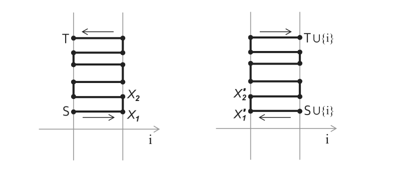
Figure 3. A coalition path from $S$ to $T$, and its reflection w.r.t. $i$.

$$\omega^{\prime}:X^{\prime}_{0}\to X^{\prime}_{1}\to\dots\to X^{\prime}_{n}$$

where $X^{\prime}_{k}:=X_{k}\cup\{i\}$ if $i\notin X_{k}$, and $X^{\prime}_{k}:=X_{k}\setminus\{i\}$ if $i\in X_{k}$. We observe that the total contribution of the player $i$ (that is, the sum of $\mathrm{d}_{i}v$’s) along the paths $\omega$ and $\omega^{\prime}$ has the opposite sign, because whenever the player $i$ joins or leaves coalition along $\omega$, $i$ leaves or joins coalition along $\omega^{\prime}$. By integrating over all paths $\omega$ traveling from $S$ to $T$, and its refection $\omega^{\prime}$ from $T$ to $S$, we deduce $V_{i}^{S\cup\{i\}}(T\cup\{i\})=-V_{i}^{S}(T)$. Utilizing the fact $V_{i}^{S}(T)=V_{i}(T)-V_{i}(S)$ (see Lemma 9.3), this is precisely (4.5).

Thus, A5 already reflects the idea that the average value of path integration should be used to determine allocation, and it provides information about the values at two different states $S,T$ in terms of their relationship with $S\cup\{i\},T\cup\{i\}$. This eventually allows us to determine all of the component values $(v_{i})_{i\in[N]}$ on ${\cal V}$.

We emphasize the distinction once more: whereas the Shapley formula (2.2) considers coalition processes in the joining direction only, our path integral formula now allows coalitions to proceed in either direction, which eventually yields a complete characterization of the values $V_{i}(S)$ for all coalitions $S$ thanks to A5. In this sense, A1–A5 can be thought of as a completion of the Shapley axioms.

5. Generalized Shapley value: $f$-Shapley value and its extension

The null-player axiom, which states that a player who contributes no marginal value to any coalition receives nothing, is arguably the most important of the Shapley axioms, serving as the key to determining the Shapley value.

It is worth noting that the Shapley value (2.2) for player $i$ can be rewritten as

(5.1) $$\phi_{i}(v)=\frac{1}{N!}\sum_{\sigma}\bigg{[}\sum_{j\in[N]}\mathrm{d}_{i}v\big{(}S^{\sigma}_{j},S^{\sigma}_{j}\cup\{j\}\big{)}\bigg{]},$$

because the only nonzero term in the path-integral, the sum over $j$ in the bracket, is when $j=i$. This indicates that the role of the coalition game $v$ is simply yielding the marginal contribution of player $i$ as the form $\mathrm{d}_{i}v$. While this may seem like a reasonable choice for player $i$’s marginal value, especially in light of Shapley’s null player axiom, we now claim that it is not the only possibility. Presumably, the only important property $\mathrm{d}_{i}v$ has is that it belongs to $\ell^{2}({\cal E})$, i.e., it satisfies the alternating property. Now we define the player $i$’s marginal value as an arbitrary edge flow $f_{i}\in\ell^{2}({\cal E})$, and contend that this is a practically relevant generalization because, in practice, even when only one player makes progress at a given cooperative stage, the reward is usually distributed to all players in the cooperation in some way.

For a player whose marginal value is given by $f\in\ell^{2}({\cal E})$, a natural generalization of the Shapley value can now be given as (cf. (5.1))

(5.2) $$\phi_{f}:=\frac{1}{N!}\sum_{\sigma}\sum_{j\in[N]}f\big{(}S^{\sigma}_{j},S^{\sigma}_{j}\cup\{j\}\big{)}.$$

Notice that the coalition game $v\in{\cal G}_{N}$ is no longer present in the formula.

On the other hand, Stern and Tettenhorst’s component game values $v_{i}:{\cal V}\to{\mathbb{R}}$ can be generalized as the unique solution $v_{f}$ to the Poisson’s equation (cf. (3.10))

(5.3) $$\mathrm{d}^{\ast}\mathrm{d}v_{f}=\mathrm{d}^{\ast}f\quad\text{with}\quad v_{f}(\emptyset)=0,$$

where $\mathrm{d}_{i}v$ is now replaced by $f$. Then analogous to Proposition 4.2, $v_{f}$ allows for the stochastic integral representation (see Theorem 7.3 for more general result)

(5.4) $$v_{f}(T)=\int_{\Omega}\sum_{n=1}^{\tau_{T}(\omega)}f\big{(}X_{n-1}(\omega),X_{n}(\omega)\big{)}d{\cal P}(\omega)={\mathbb{E}}\bigg{[}\sum_{n=1}^{\tau_{T}}f\big{(}X_{n-1},X_{n}\big{)}\bigg{]},$$

again allowing us to interpret $v_{f}(T)$ as the player’s expected total contribution, thus her fair share, if the coalition state advances from $\emptyset$ to $T$ and the player’s marginal contribution for each transition is now given by an arbitrary edge flow $f$.

We can now generalize the coincidence result (3.11) into the following.

Proposition 5.1.

$\phi_{f}=v_{f}([N])$  for any edge flow $f$ on the coalition game graph.

Notice (3.11) becomes a special case precisely when $f$ is given by $\mathrm{d}_{i}v$ for $v\in{\cal G}_{N}$. In light of the proposition, we may call $\phi_{f}$ the $f$-Shapley value, with $v_{f}:{\cal V}\to{\mathbb{R}}$ its extension to all partial coalition states.

An example of “less-strict” marginal value allocation may be given as follows. Given $\alpha\in{\mathbb{R}}$, $N$ players and a coalition game $v\in{\cal G}_{N}$, let us define player $i$’s marginal value by (cf. (3.9))

(5.5) $$f_{\alpha,i}\bigl{(}S,S\cup\{j\}\bigr{)}:=\begin{cases}\alpha\big{(}v(S\cup\{i\})-v(S)\big{)}&\text{if }\ j=i,\\ \frac{(1-\alpha)}{N-1}\big{(}v(S\cup\{j\})-v(S)\big{)}&\text{if }\ j\neq i.\end{cases}$$

Note that $f_{\alpha,i}=\mathrm{d}_{i}v$ if $\alpha=1$. For $\alpha\in(0,1)$, the marginal value allocation scheme (5.5) is such that for the transition from $S$ to $S\cup\{i\}$, player $i$ receives the $\alpha$ proportion of the marginal value $v(S\cup\{i\})-v(S)$, and the rest of the value $(1-\alpha)\big{(}v(S\cup\{i\})-v(S)\big{)}$ is equally distributed to the rest of the players $[N]\setminus\{i\}$. We may call $\phi_{f_{\alpha,i}}$ the $\alpha$-Shapley value, with $v_{f_{\alpha,i}}$ its extension. Now the null-player axiom may not hold for the $\alpha$-Shapley value, as the following example shows.

Example 5.2.

Let $N=2$, and $v\in{\cal G}_{2}$ be given by $v(\emptyset)=v(\{2\})=0$, $v(\{1\})=v(\{1,2\})=1$. Note that $\mathrm{d}_{2}v=0$, thus the Shapley value $\phi_{2}(v)=0$ for player 2. On the other hand, the $\alpha$-Shapley value for player 2 can be easily calculated as $1-\alpha$. Player 2 continues to receive the $1-\alpha$ portion of the grand coalition value.

We now examine the values (5.2) and (5.4) in the context of the glove game.

Example 5.3 (Glove game revisited).

We revisit the glove game from Example 2.2 and calculate the the values (5.2) and (5.4), but this time with modified marginal values of players (5.5). For $\alpha$-Shapley values, we should calculate, with $f_{i}:=f_{\alpha,i}$,

$$\phi_{\alpha,i}(v)=\frac{1}{6}\sum_{\sigma}\big{[}f_{i}(\emptyset,\{\sigma(1)\})+f_{i}(\{\sigma(1)\},\{\sigma(1),\sigma(2)\})+f_{i}(\{\sigma(1),\sigma(2)\},\{1,2,3\})\big{]},$$

where $f_{i}(\emptyset,\{\sigma(1)\})+f_{i}(\{\sigma(1)\},\{\sigma(1),\sigma(2)\})+f_{i}(\{\sigma(1),\sigma(2)\},\{1,2,3\})$ represents the total contribution of player $i$ along the coalition path $\sigma$. For example, if $\sigma=(1,2,3)$ (that is, the player $1$ joins first, followed by the players $2$ and $3$), this sum equals $\frac{1-\alpha}{2}$ for $i=1,3$ and $\alpha$ for $i=2$, because a pair of gloves is made precisely when the player $2$ joins in this path. Thus, player $1$ contributes marginal value $\frac{1-\alpha}{2}$ when joining the coalition first (2 of 6 permutations) and marginal value $\alpha$ otherwise (4 of 6 permutations), so $\phi_{\alpha,1}(v)=\frac{1+3\alpha}{6}$. Efficiency and symmetry then yield $\phi_{\alpha,2}(v)=\phi_{\alpha,3}(v)=\frac{5-3\alpha}{12}$. We notice this allocation coincides with the Shapley value if $\alpha=1$, and player $1$ receives more than players $2,3$ if and only if $\alpha>\frac{1}{3}$.

For the extended allocation (5.4), we need to solve the Poisson’s equation

(5.6) $$\mathrm{d}^{\ast}\mathrm{d}v_{f_{i}}=\mathrm{d}^{\ast}f_{i}\ \text{ with initial condition }\ v_{f_{i}}(\emptyset)=0,\quad i=1,2,3.$$

Let us denote the vertices of the unit cube by $n_{0}=(0,0,0)$, $n_{1}=(1,0,0)$, $n_{2}=(0,1,0)$, $n_{3}=(0,0,1)$, $n_{4}=(1,1,0)$, $n_{5}=(1,0,1)$, $n_{6}=(0,1,1)$, $n_{7}=(1,1,1)$. The matrix representation of $\mathrm{d}$ and the marginal values $f_{1},f_{2},f_{3}$ are given by

$$\hbox{}\vbox{\kern 0.86108pt\hbox{$\kern 0.0pt\kern 2.5pt\kern-5.0pt\left[\kern 0.0pt\kern-2.5pt\kern-5.55557pt\vbox{\kern-0.86108pt\vbox{\vbox{ \halign{\kern\arraycolsep\hfil\@arstrut$\kbcolstyle#$\hfil\kern\arraycolsep& \kern\arraycolsep\hfil$\@kbrowstyle#$\ifkbalignright\relax\else\hfil\fi\kern\arraycolsep&& \kern\arraycolsep\hfil$\@kbrowstyle#$\ifkbalignright\relax\else\hfil\fi\kern\arraycolsep\cr 5.0pt\hfil\@arstrut$\scriptstyle$\hfil\kern 5.0pt&5.0pt\hfil$\scriptstyle n_{0}$\hfil\kern 5.0pt&5.0pt\hfil$\scriptstyle n_{1}$\hfil\kern 5.0pt&5.0pt\hfil$\scriptstyle n_{2}$\hfil\kern 5.0pt&5.0pt\hfil$\scriptstyle n_{3}$\hfil\kern 5.0pt&5.0pt\hfil$\scriptstyle n_{4}$\hfil\kern 5.0pt&5.0pt\hfil$\scriptstyle n_{5}$\hfil\kern 5.0pt&5.0pt\hfil$\scriptstyle n_{6}$\hfil\kern 5.0pt&5.0pt\hfil$\scriptstyle n_{7}\\(n_{0},n_{1})$\hfil\kern 5.0pt&5.0pt\hfil$\scriptstyle-1$\hfil\kern 5.0pt&5.0pt\hfil$\scriptstyle 1$\hfil\kern 5.0pt&5.0pt\hfil$\scriptstyle 0$\hfil\kern 5.0pt&5.0pt\hfil$\scriptstyle 0$\hfil\kern 5.0pt&5.0pt\hfil$\scriptstyle 0$\hfil\kern 5.0pt&5.0pt\hfil$\scriptstyle 0$\hfil\kern 5.0pt&5.0pt\hfil$\scriptstyle 0$\hfil\kern 5.0pt&5.0pt\hfil$\scriptstyle 0\\(n_{0},n_{2})$\hfil\kern 5.0pt&5.0pt\hfil$\scriptstyle-1$\hfil\kern 5.0pt&5.0pt\hfil$\scriptstyle 0$\hfil\kern 5.0pt&5.0pt\hfil$\scriptstyle 1$\hfil\kern 5.0pt&5.0pt\hfil$\scriptstyle 0$\hfil\kern 5.0pt&5.0pt\hfil$\scriptstyle 0$\hfil\kern 5.0pt&5.0pt\hfil$\scriptstyle 0$\hfil\kern 5.0pt&5.0pt\hfil$\scriptstyle 0$\hfil\kern 5.0pt&5.0pt\hfil$\scriptstyle 0\\(n_{0},n_{3})$\hfil\kern 5.0pt&5.0pt\hfil$\scriptstyle-1$\hfil\kern 5.0pt&5.0pt\hfil$\scriptstyle 0$\hfil\kern 5.0pt&5.0pt\hfil$\scriptstyle 0$\hfil\kern 5.0pt&5.0pt\hfil$\scriptstyle 1$\hfil\kern 5.0pt&5.0pt\hfil$\scriptstyle 0$\hfil\kern 5.0pt&5.0pt\hfil$\scriptstyle 0$\hfil\kern 5.0pt&5.0pt\hfil$\scriptstyle 0$\hfil\kern 5.0pt&5.0pt\hfil$\scriptstyle 0\\(n_{1},n_{4})$\hfil\kern 5.0pt&5.0pt\hfil$\scriptstyle 0$\hfil\kern 5.0pt&5.0pt\hfil$\scriptstyle-1$\hfil\kern 5.0pt&5.0pt\hfil$\scriptstyle 0$\hfil\kern 5.0pt&5.0pt\hfil$\scriptstyle 0$\hfil\kern 5.0pt&5.0pt\hfil$\scriptstyle 1$\hfil\kern 5.0pt&5.0pt\hfil$\scriptstyle 0$\hfil\kern 5.0pt&5.0pt\hfil$\scriptstyle 0$\hfil\kern 5.0pt&5.0pt\hfil$\scriptstyle 0\\(n_{2},n_{4})$\hfil\kern 5.0pt&5.0pt\hfil$\scriptstyle 0$\hfil\kern 5.0pt&5.0pt\hfil$\scriptstyle 0$\hfil\kern 5.0pt&5.0pt\hfil$\scriptstyle-1$\hfil\kern 5.0pt&5.0pt\hfil$\scriptstyle 0$\hfil\kern 5.0pt&5.0pt\hfil$\scriptstyle 1$\hfil\kern 5.0pt&5.0pt\hfil$\scriptstyle 0$\hfil\kern 5.0pt&5.0pt\hfil$\scriptstyle 0$\hfil\kern 5.0pt&5.0pt\hfil$\scriptstyle 0\\(n_{1},n_{5})$\hfil\kern 5.0pt&5.0pt\hfil$\scriptstyle 0$\hfil\kern 5.0pt&5.0pt\hfil$\scriptstyle-1$\hfil\kern 5.0pt&5.0pt\hfil$\scriptstyle 0$\hfil\kern 5.0pt&5.0pt\hfil$\scriptstyle 0$\hfil\kern 5.0pt&5.0pt\hfil$\scriptstyle 0$\hfil\kern 5.0pt&5.0pt\hfil$\scriptstyle 1$\hfil\kern 5.0pt&5.0pt\hfil$\scriptstyle 0$\hfil\kern 5.0pt&5.0pt\hfil$\scriptstyle 0\\(n_{3},n_{5})$\hfil\kern 5.0pt&5.0pt\hfil$\scriptstyle 0$\hfil\kern 5.0pt&5.0pt\hfil$\scriptstyle 0$\hfil\kern 5.0pt&5.0pt\hfil$\scriptstyle 0$\hfil\kern 5.0pt&5.0pt\hfil$\scriptstyle-1$\hfil\kern 5.0pt&5.0pt\hfil$\scriptstyle 0$\hfil\kern 5.0pt&5.0pt\hfil$\scriptstyle 1$\hfil\kern 5.0pt&5.0pt\hfil$\scriptstyle 0$\hfil\kern 5.0pt&5.0pt\hfil$\scriptstyle 0\\(n_{2},n_{6})$\hfil\kern 5.0pt&5.0pt\hfil$\scriptstyle 0$\hfil\kern 5.0pt&5.0pt\hfil$\scriptstyle 0$\hfil\kern 5.0pt&5.0pt\hfil$\scriptstyle-1$\hfil\kern 5.0pt&5.0pt\hfil$\scriptstyle 0$\hfil\kern 5.0pt&5.0pt\hfil$\scriptstyle 0$\hfil\kern 5.0pt&5.0pt\hfil$\scriptstyle 0$\hfil\kern 5.0pt&5.0pt\hfil$\scriptstyle 1$\hfil\kern 5.0pt&5.0pt\hfil$\scriptstyle 0\\(n_{3},n_{6})$\hfil\kern 5.0pt&5.0pt\hfil$\scriptstyle 0$\hfil\kern 5.0pt&5.0pt\hfil$\scriptstyle 0$\hfil\kern 5.0pt&5.0pt\hfil$\scriptstyle 0$\hfil\kern 5.0pt&5.0pt\hfil$\scriptstyle-1$\hfil\kern 5.0pt&5.0pt\hfil$\scriptstyle 0$\hfil\kern 5.0pt&5.0pt\hfil$\scriptstyle 0$\hfil\kern 5.0pt&5.0pt\hfil$\scriptstyle 1$\hfil\kern 5.0pt&5.0pt\hfil$\scriptstyle 0\\(n_{4},n_{7})$\hfil\kern 5.0pt&5.0pt\hfil$\scriptstyle 0$\hfil\kern 5.0pt&5.0pt\hfil$\scriptstyle 0$\hfil\kern 5.0pt&5.0pt\hfil$\scriptstyle 0$\hfil\kern 5.0pt&5.0pt\hfil$\scriptstyle 0$\hfil\kern 5.0pt&5.0pt\hfil$\scriptstyle-1$\hfil\kern 5.0pt&5.0pt\hfil$\scriptstyle 0$\hfil\kern 5.0pt&5.0pt\hfil$\scriptstyle 0$\hfil\kern 5.0pt&5.0pt\hfil$\scriptstyle 1\\(n_{5},n_{7})$\hfil\kern 5.0pt&5.0pt\hfil$\scriptstyle 0$\hfil\kern 5.0pt&5.0pt\hfil$\scriptstyle 0$\hfil\kern 5.0pt&5.0pt\hfil$\scriptstyle 0$\hfil\kern 5.0pt&5.0pt\hfil$\scriptstyle 0$\hfil\kern 5.0pt&5.0pt\hfil$\scriptstyle 0$\hfil\kern 5.0pt&5.0pt\hfil$\scriptstyle-1$\hfil\kern 5.0pt&5.0pt\hfil$\scriptstyle 0$\hfil\kern 5.0pt&5.0pt\hfil$\scriptstyle 1\\(n_{6},n_{7})$\hfil\kern 5.0pt&5.0pt\hfil$\scriptstyle 0$\hfil\kern 5.0pt&5.0pt\hfil$\scriptstyle 0$\hfil\kern 5.0pt&5.0pt\hfil$\scriptstyle 0$\hfil\kern 5.0pt&5.0pt\hfil$\scriptstyle 0$\hfil\kern 5.0pt&5.0pt\hfil$\scriptstyle 0$\hfil\kern 5.0pt&5.0pt\hfil$\scriptstyle 0$\hfil\kern 5.0pt&5.0pt\hfil$\scriptstyle-1$\hfil\kern 5.0pt&5.0pt\hfil$\scriptstyle 1$\hfil\kern 5.0pt\crcr}}}}\right]$}},\quad\hbox{}\vbox{\kern 0.86108pt\hbox{$\kern 0.0pt\kern 2.5pt\kern-5.0pt\left[\kern 0.0pt\kern-2.5pt\kern-5.55557pt\vbox{\kern-0.86108pt\vbox{\vbox{ \halign{\kern\arraycolsep\hfil\@arstrut$\kbcolstyle#$\hfil\kern\arraycolsep& \kern\arraycolsep\hfil$\@kbrowstyle#$\ifkbalignright\relax\else\hfil\fi\kern\arraycolsep&& \kern\arraycolsep\hfil$\@kbrowstyle#$\ifkbalignright\relax\else\hfil\fi\kern\arraycolsep\cr 5.0pt\hfil\@arstrut$\scriptstyle$\hfil\kern 5.0pt&5.0pt\hfil$\scriptstyle f_{1}$\hfil\kern 5.0pt&5.0pt\hfil$\scriptstyle f_{2}$\hfil\kern 5.0pt&5.0pt\hfil$\scriptstyle f_{3}\\(n_{0},n_{1})$\hfil\kern 5.0pt&5.0pt\hfil$\scriptstyle 0$\hfil\kern 5.0pt&5.0pt\hfil$\scriptstyle 0$\hfil\kern 5.0pt&5.0pt\hfil$\scriptstyle 0\\(n_{0},n_{2})$\hfil\kern 5.0pt&5.0pt\hfil$\scriptstyle 0$\hfil\kern 5.0pt&5.0pt\hfil$\scriptstyle 0$\hfil\kern 5.0pt&5.0pt\hfil$\scriptstyle 0\\(n_{0},n_{3})$\hfil\kern 5.0pt&5.0pt\hfil$\scriptstyle 0$\hfil\kern 5.0pt&5.0pt\hfil$\scriptstyle 0$\hfil\kern 5.0pt&5.0pt\hfil$\scriptstyle 0\\(n_{1},n_{4})$\hfil\kern 5.0pt&5.0pt\hfil$\scriptstyle\frac{1-\alpha}{2}$\hfil\kern 5.0pt&5.0pt\hfil$\scriptstyle\alpha$\hfil\kern 5.0pt&5.0pt\hfil$\scriptstyle\frac{1-\alpha}{2}\\(n_{2},n_{4})$\hfil\kern 5.0pt&5.0pt\hfil$\scriptstyle\alpha$\hfil\kern 5.0pt&5.0pt\hfil$\scriptstyle\frac{1-\alpha}{2}$\hfil\kern 5.0pt&5.0pt\hfil$\scriptstyle\frac{1-\alpha}{2}\\(n_{1},n_{5})$\hfil\kern 5.0pt&5.0pt\hfil$\scriptstyle\frac{1-\alpha}{2}$\hfil\kern 5.0pt&5.0pt\hfil$\scriptstyle\frac{1-\alpha}{2}$\hfil\kern 5.0pt&5.0pt\hfil$\scriptstyle\alpha\\(n_{3},n_{5})$\hfil\kern 5.0pt&5.0pt\hfil$\scriptstyle\alpha$\hfil\kern 5.0pt&5.0pt\hfil$\scriptstyle\frac{1-\alpha}{2}$\hfil\kern 5.0pt&5.0pt\hfil$\scriptstyle\frac{1-\alpha}{2}\\(n_{2},n_{6})$\hfil\kern 5.0pt&5.0pt\hfil$\scriptstyle 0$\hfil\kern 5.0pt&5.0pt\hfil$\scriptstyle 0$\hfil\kern 5.0pt&5.0pt\hfil$\scriptstyle 0\\(n_{3},n_{6})$\hfil\kern 5.0pt&5.0pt\hfil$\scriptstyle 0$\hfil\kern 5.0pt&5.0pt\hfil$\scriptstyle 0$\hfil\kern 5.0pt&5.0pt\hfil$\scriptstyle 0\\(n_{4},n_{7})$\hfil\kern 5.0pt&5.0pt\hfil$\scriptstyle 0$\hfil\kern 5.0pt&5.0pt\hfil$\scriptstyle 0$\hfil\kern 5.0pt&5.0pt\hfil$\scriptstyle 0\\(n_{5},n_{7})$\hfil\kern 5.0pt&5.0pt\hfil$\scriptstyle 0$\hfil\kern 5.0pt&5.0pt\hfil$\scriptstyle 0$\hfil\kern 5.0pt&5.0pt\hfil$\scriptstyle 0\\(n_{6},n_{7})$\hfil\kern 5.0pt&5.0pt\hfil$\scriptstyle\alpha$\hfil\kern 5.0pt&5.0pt\hfil$\scriptstyle\frac{1-\alpha}{2}$\hfil\kern 5.0pt&5.0pt\hfil$\scriptstyle\frac{1-\alpha}{2}$\hfil\kern 5.0pt\crcr}}}}\right]$}},$$

with $\mathrm{d}^{\ast}$ represented by the transpose matrix of $\mathrm{d}$. $L=\mathrm{d}^{\ast}\mathrm{d}$ represents the Laplacian. In view of the initial condition, we need to solve $L_{0}w_{i}=\mathrm{d}^{\ast}f_{i}$, where $L_{0}$ is a $8\times 7$ matrix equal to $L$ with the first column removed; then $w_{i}\in{\mathbb{R}}^{7}$ coincides with $v_{i}$ for each nonempty $S\subseteq\{1,2,3\}$. Since $w_{i}$ is unique, it is given by

(5.7) $$w_{i}=(L_{0}^{\ast}L_{0})^{-1}L_{0}^{\ast}\mathrm{d}^{\ast}f_{i},\quad i=1,2,3.$$

Solving (5.7), we obtain the following extended allocation table.

	$\{1\}$	$\{2\}$	$\{3\}$	$\{1,2\}$	$\{1,3\}$	$\{2,3\}$	$\{1,2,3\}$
$v_{f_{1}}$	$-\frac{5}{24}+\frac{5\alpha}{8}$	$\frac{5}{48}-\frac{5\alpha}{16}$	$\frac{5}{48}-\frac{5\alpha}{16}$	$\frac{3}{16}+\frac{7\alpha}{16}$	$\frac{3}{16}+\frac{7\alpha}{16}$	$\frac{1}{8}-\frac{3\alpha}{8}$	$\frac{1}{6}+\frac{\alpha}{2}$
$v_{f_{2}}$	$\frac{5}{48}-\frac{5\alpha}{16}$	$-\frac{1}{12}+\frac{\alpha}{4}$	$-\frac{1}{48}+\frac{\alpha}{16}$	$\frac{5}{16}+\frac{\alpha}{16}$	$\frac{1}{2}-\frac{\alpha}{2}$	$-\frac{1}{16}+\frac{3\alpha}{16}$	$\frac{5}{12}-\frac{\alpha}{4}$
$v_{f_{3}}$	$\frac{5}{48}-\frac{5\alpha}{16}$	$-\frac{1}{48}+\frac{\alpha}{16}$	$-\frac{1}{12}+\frac{\alpha}{4}$	$\frac{1}{2}-\frac{\alpha}{2}$	$\frac{5}{16}+\frac{\alpha}{16}$	$-\frac{1}{16}+\frac{3\alpha}{16}$	$\frac{5}{12}-\frac{\alpha}{4}$

We see that $v_{f_{i}}(\{1,2,3\})=\phi_{\alpha,i}(v)$; the extended allocation at the grand coalition coincides with the $\alpha$-Shapley value, as claimed in Proposition 5.1.

The author believes that finding generalized Shapley axioms that can characterize the extended allocation scheme corresponding to the marginal value (5.5) and many other possible choices is an interesting question for future research.

6. Generalized Nash-Kohlberg-Neyman’s value for strategic games

In this section, we further explore the economic significance of our findings by discussing the Nash’s and Kohlberg–Neyman’s value allocation scheme for the strategic cooperative games, and explaining how their axiomatic notion of value can be reinterpreted and extended to all partial coalitions using the theory we have developed thus far.

According to Kohlberg and Neyman [11], a strategic game is a model for a multiperson competitive interaction. Each player chooses a strategy, and the combined choices of all the players determine a payoff to each of them. A problem of interest in game theory is the following: How to evaluate, in advance of playing a game, the economic worth of a player’s position? A “value” is a general solution, that is, a method for evaluating the worth of any player in a given strategic game.

According to [11], a strategic game is defined by a triple $G=([N],A,g)$, where

$\cdot$ $[N]=\{1,2,...,N\}$ is a finite set of players,

$\cdot$ $A^{i}$ is the finite set of player $i$’s pure strategies, and $A=\prod_{i=1}^{N}A^{i}$,

$\cdot$ $g^{i}:A\to{\mathbb{R}}$ is player $i$’s payoff function, and $g=(g^{i})_{i\in[N]}$.

The same notation, $g$, is used to denote the linear extension

$\cdot$ $g^{i}:\Delta(A)\to{\mathbb{R}}$, where for any set $K$, $\Delta(K)$ denotes the probability distributions over $K$.

For each coalition $S\subseteq[N]$, we also denote

$\cdot$ $A^{S}=\prod_{i\in S}A^{i}$, and

$\cdot$ $X^{S}=\Delta(A^{S})$   (correlated strategies of the players in $S$).

Let $\mathbb{G}([N])$ be the set of all $N$-player strategic games. Consider $\gamma:\mathbb{G}([N])\to{\mathbb{R}}^{N}$ that associates with any strategic game an allocation of payoffs to the players. Now, Kohlberg and Neyman [11] proposed a set of axioms for characterizing $\gamma$, the core concept of which is the following definition of the threat power of coalition $S$:

(6.1) $$(\delta G)(S):=\max_{x\in X^{S}}\min_{y\in X^{[N]\setminus S}}\bigg{(}\sum_{i\in S}g^{i}(x,y)-\sum_{i\notin S}g^{i}(x,y)\bigg{)}.$$

The threat power of $S$ (to the other party $[N]\setminus S$) can be read as the maximum difference between the sum of the players’ payoffs in $S$ and the sum of the other party’s payoffs, regardless of what collective strategies the other party employs.

Then Kohlberg and Neyman demonstrated that the axioms of Efficiency (the sum of all players’ payoffs, i.e., $(\delta G)([N])$, is fully distributed among the players), Balanced threats (see below), Symmetry (equivalent players receive equal amounts), Null player (a player having no strategic impact on players’ payoffs has zero value), and Additivity (the allocation is additive on strategic games) uniquely determine an allocation $\gamma$; see [11] for details. Moreover, they showed that such allocation $\gamma$ generalizes the Nash solution for two-person games [21] into $N$-person games.

Among the axioms, the key axiom of balanced threats asserts the following:

$\cdot$ If $(\delta G)(S)=0$ for all $S\subseteq[N]$, then $\gamma_{i}=0$ for all $i\in[N]$.

Namely, if no coalition $S$ has threat power over the other party, the allocation is zero for all players. From now on, let $\gamma=(\gamma_{1},...,\gamma_{N})$ denote the unique allocation determined by the above five axioms. [11] then provides an explicit formula for $\gamma$:

(6.2) $$\gamma_{i}G=\frac{1}{N!}\sum_{\sigma}(\delta G)\big{(}\bar{S}^{\sigma}_{i}\big{)},$$

where the summation is over all permutations $\sigma$ of the set $[N]$, $S^{\sigma}_{i}$ is the subset consisting of those $j\in[N]$ that precede $i$ in the ordering $\sigma$, and $\bar{S}^{\sigma}_{i}:=S^{\sigma}_{i}\cup\{i\}$.

Now we will focus on the value allocation formula (6.2) and manipulate it as follows. By minimax principle, it is easily seen that $(\delta G)(S)=-(\delta G)([N]\setminus S)$. This antisymmetry implies

$$\gamma_{i}G =\frac{1}{N!}\sum_{\sigma}\frac{(\delta G)\big{(}\bar{S}^{\sigma}_{i}\big{)}-(\delta G)\big{(}[N]\setminus\bar{S}^{\sigma}_{i}\big{)}}{2}$$

$$=\frac{1}{2N!}\sum_{\sigma}(\delta G)\big{(}\bar{S}^{\sigma}_{i}\big{)}-\frac{1}{2N!}\sum_{\sigma}(\delta G)\big{(}[N]\setminus\bar{S}^{\sigma}_{i}\big{)}$$

(6.3) $$=\frac{1}{2N!}\sum_{\sigma}(\delta G)\big{(}\bar{S}^{\sigma}_{i}\big{)}-\frac{1}{2N!}\sum_{\sigma}(\delta G)\big{(}S^{\sigma}_{i}\big{)}.$$

Motivated by this, let us define the coalition game $v=v_{G}:2^{[N]}\to{\mathbb{R}}$ as follows:

(6.4) $$v(S):=\frac{(\delta G)(S)+(\delta G)([N])}{2}=\frac{(\delta G)([N])-(\delta G)([N]\setminus S)}{2}.$$

The value function $v(S)$ may be interpreted as the grand coalition value $(\delta G)([N])$ subtracted by the threat power of the other party $[N]\setminus S$, with a factor of 1/2.

By the fact that the value function $v$ is simply a translation of $\delta G/2$, we have

(6.5) $$\mathrm{d}_{i}v(S^{\sigma}_{i})=v(\bar{S}^{\sigma}_{i})-v(S^{\sigma}_{i})=\frac{(\delta G)\big{(}\bar{S}^{\sigma}_{i}\big{)}-(\delta G)\big{(}S^{\sigma}_{i}\big{)}}{2}.$$

In view of (6.3), we arrive at the following alternative expression for $\gamma_{i}G$:

(6.6) $$\gamma_{i}G=\frac{1}{N!}\sum_{\sigma}\mathrm{d}_{i}v(S^{\sigma}_{i}).$$

We observe that this is the Shapley value (2.2) for the coalition game $v=v_{G}$. Then we recall that [31] defines the component game $v_{i}$ for each $i\in[N]$ as the unique solution in ${\cal G}_{N}$ to the equation $\mathrm{d}^{\ast}\mathrm{d}v_{i}=\mathrm{d}^{\ast}\mathrm{d}_{i}v$, and shows that the component game value at the grand coalition coincides with the Shapley value, that is, $v_{i}([N])=\gamma_{i}G$ in this context. With this, Proposition 4.2 now allows us to conclude the following.

Theorem 6.1 (Parametrized extension of Kohlberg–Neyman’s value to all states).

Given a strategic game $G\in\mathbb{G}([N])$, let $v\in{\cal G}(2^{[N]})$ be the coalition game defined by (6.4). Let $\alpha\in{\mathbb{R}}$, and $(X_{n})_{n\in{\mathbb{N}}_{0}}$ denote the coalition process (4.1) with $X_{0}=\emptyset$. Then for each player $i\in[N]$ and coalition $S\subseteq[N]$, the value allocation operator

$$V_{\alpha,i}(S):={\mathbb{E}}\bigg{[}\sum_{n=1}^{\tau_{S}}f_{\alpha,i}\big{(}X_{n-1},X_{n}\big{)}\bigg{]}$$

where $f_{\alpha,i}$ is given by (5.5), extends Kohlberg–Neyman’s value in the sense that $V_{1,i}([N])=\gamma_{i}G$. Furthermore, if $\alpha=1$, the conditions A1–A5 in Theorem (4.1) characterizes the value $V_{1,i}(S)$ for all coalitions $S\subseteq[N]$, including the value $\gamma_{i}G$.

Proof.

[31] showed $v_{i}([N])=\gamma_{i}G$, where $v_{i}\in{\cal G}_{N}$ is the solution to (3.10). Proposition 5.1 then yields $v_{i}=V_{1,i}$ on $2^{[N]}$. The final claim follows from Theorem 4.1. ∎

We note that Kohlberg and Neyman also introduce the concept of Bayesian games, which is a game of incomplete information in the sense that the players do not know the true payoff functions, but only receive a signal that is correlated with the payoff functions; see [11] for details. In this context, the threat power, $(\delta_{B}G)(S)$, of a coalition $S$ in the Bayesian game $G$ remains antisymmetric, i.e., $(\delta_{B}G)(S)=-(\delta_{B}G)([N]\setminus S)$, and the value allocation also satisfies the representation formula (6.2). As a result, we can conclude that the value of Bayesian games still admits the stochastic path-integral extension for all coalitions, as shown in Theorem 6.1.

We should note that this section only attempted to summarize some of the key concepts of Kohlberg and Neyman’s work; fully explaining it is beyond the scope of this paper and the author’s ability. Instead, we refer to [11, 12] for a comprehensive development of the concept of value and a detailed review of the historical development of ideas surrounding it, as well as several applications to various economic models.

7. Generalized cooperative network and Hodge allocation

So far, we have made generalizations of Shapley’s cooperative value allocation theory in various ways, with the key idea being the consideration of the coalition game graph (3.1), the Poisson’s equation (5.3), and its stochastic path integral solution representation (5.4). Nonetheless, this keeps prompting the author to ask: why should we limit ourselves to the coalition game graph?

While the equation (3.10) considered in [31] cannot be defined on a general graph due to the presence of the partial differentiation operator $\mathrm{d}_{i}v$, which requires the hypercube graph structure, our generalization (5.3) can. This leads us to consider a cooperative game graph $G=({\cal V},{\cal E})$, which is a general connected graph with ${\cal V}$ a finite set of states and ${\cal E}$ a set of edges. It should be noted that now each $S\in{\cal V}$ is not necessarily a subset of $[N]$, but ${\cal V}$ now represents an arbitrary finite set, with each $S\in{\cal V}$ describing a general cooperative situation. For example, $S,T\in{\cal V}$ may both represent cooperations among the same group of players but working under different conditions and/or producing different outcomes, and so on.

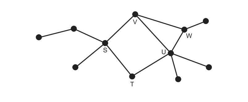
Figure 4. A cooperative graph can have an arbitrary structure. Each edge has a forward and reverse direction associated to it.

As an example of the situation of interest, we may consider the following: Let ${\cal V}$ represent the set of all possible states of a given project, in which the project manager, or principal, wishes to reach the project completion state $F\in{\cal V}$. The state can move from $S$ to $T$ with a certain probability, if there is an edge between them. For the project’s advancement, the manager hires $N$ agents, or employees.

Question: Given the principal’s reward function in each state and her payoff function to agents at each state transition, what is her expected revenue when the project is completed, and what is her expected liability to each agent?

The question naturally prompts us to consider a general Markov chain $(X^{U}_{n})_{n\in{\mathbb{N}}_{0}}$ on the state space ${\cal V}$ with initial state $X_{0}=U$, which is governed by the transition probability $p_{S,T}$ which expresses the likelihood of a transition from a state $S$ to $T$.

Let $(S,T)\in{\cal E}$ denote a forward edge directed from $S$ to $T$, with its reverse $(T,S)\in{\cal E}_{-}$. Set $\overline{\cal E}:={\cal E}\cup{\cal E}_{-}$. Let $\ell^{2}({\cal E})$ represent the set of edge flows $f:\overline{\cal E}\to{\mathbb{R}}$ satisfying the alternating property $f(T,S)=-f(S,T)$. Motivated from Section 5, we continue to assume that each agent $i=1,2,...,N$ is associated with an edge flow $f_{i}\in\ell^{2}({\cal E})$, which represents the agent $i$’s marginal contribution measure.

Let $(\Omega,{\cal F},{\cal P})$ denote the underlying probability space for the Markov chain. For each $S,T\in{\cal V}$ and a sample path $\omega\in\Omega$, let $\tau_{T}=\tau_{T}(\omega)\in{\mathbb{N}}$ denote the first (random) time the Markov chain $\big{(}X^{S}_{n}(\omega)\big{)}_{n}$ visits $T$. We assume $\tau\geq 1$; if Markov chain starts at $T$, then $\tau_{T}$ denotes the Markov chain’s first return time to $T$.

Given a $f\in\ell^{2}({\cal E})$ which represents a marginal value of an agent, we then define the agent’s total contribution along the sample path $\omega$ traveling from $S$ to $T$ by

(7.1) $${\cal I}_{f}^{S}(T)={\cal I}_{f}^{S}(T)(\omega):=\sum_{n=1}^{\tau_{T}(\omega)}f\big{(}X^{S}_{n-1}(\omega),X^{S}_{n}(\omega)\big{)}.$$

The space ${\cal V}$ can represent all possible project progress states, and $f(U,V)$ represents the marginal contribution value of an agent when the state moves from $U$ to a neighbor state $V$. Given that the project state has progressed from $S$ to $T$ along the path $\omega$, (7.1) represents the agent’s total contribution throughout the progression. In view of this, we can refer to the Markov chain as a cooperative process. The value function can then be defined via the stochastic path integral

(7.2) $$V_{f}^{S}(T):=\int_{\Omega}{\cal I}_{f}^{S}(T)(\omega)d{\cal P}(\omega)={\mathbb{E}}[{\cal I}_{f}^{S}(T)].$$

$V_{f}^{S}(T)$ represents the agent’s expected total contribution if the state advances from $S$ to $T$, where $f$ represents the agent’s marginal contribution for each transition.

We can now provide a general answer to the question as follows. Let ${\cal V}$ represent the project state space in which the manager wishes to achieve the project completion state $F\in{\cal V}$. Let $v:{\cal V}\to{\mathbb{R}}$ denote the manager’s revenue, i.e., $v(U)$ represents the manager’s revenue if the project terminates at the state $U$. Let $[N]=\{1,...,N\}$ denote the employees with their marginal contribution measures $f_{1},...,f_{N}\in\ell^{2}({\cal E})$. Because it is her contribution and share, the manager must pay $f_{i}(S,T)$ to the employee $i$ at each state transition from $S$ to $T$. Thus, the manager’s surplus in this single transition is given by $v(T)-v(S)-\sum_{i}f_{i}(S,T)$.

Now the manager’s revenue problem is: What is the manager’s expected revenue if they begin at the initial project state (say $O$, where we may assume $v(O)=0$) and the manager’s goal is to reach the project completion state $F$?

We can observe that the answer is $v(F)-\sum_{i}V^{O}_{f_{i}}(F)$, where $V^{O}_{f_{i}}$ is given by (7.2). (So if this is negative, the manager may decide not to begin the project at all.)

Furthermore, in the middle of the project, the manager may want to recalculate her expected gain or loss. That is, suppose the current project status is $T$, and they arrived at $T$ via a specific path $\omega$, and thus the manager has paid the payoffs, i.e., the path integrals (7.1), to the employees. The manager may wish to recalculate the expected gain if she decides to proceed from $T$ to $F$. This is now provided by

$$v(F)-v(T)-\sum_{i}V^{T}_{f_{i}}(F),$$

and the manager can make decisions based on the expected revenue information.

Remark 7.1 (On efficiency).

Shapley’s efficiency axiom is a crucial ingredient for characterizing his value allocation scheme; without it, it is difficult to establish the uniqueness of the allocation. The efficiency axiom is equally important for our new set of axioms to produce a unique allocation for each partial coalition state.

Our description of the principal-agent allocation problem, on the other hand, shows that efficiency is merely a constraint, which is equivalent to declaring that the principal’s marginal surplus $v(T)-v(S)-\sum_{i}f_{i}(S,T)$ is identically zero for every $(S,T)\in\overline{\cal E}$. The principal enters the problem as soon as we relax this vanishing constraint, and $v:{\cal V}\to{\mathbb{R}}$ then represents her value at each cooperative state. The crucial difference between principal and agents is that the value of the principal is represented as a function on ${\cal V}$, whereas the (marginal) value of the agents is represented as edge flows on $\overline{\cal E}$. Finally, we can recover the efficiency condition by imposing the condition $\mathrm{d}v=\sum_{i}f_{i}$, as was the case for the $\alpha$-Shapley value (5.5).

As an example of a general cooperative game network, we may describe the merger game graph, which differs significantly from the coalition game graph (3.1).

Example 7.2 (Merger game graph).

Given $[N]=\{1,2,...,N\}$ the set of players, we consider a graph $G=({\cal V},{\cal E})$ where each $S\in{\cal V}$ describes a partition of $[N]$. For example, if $N=6$, then $U=\{\{1,2\},\{3,4,5\},\{6\}\}$, $V=\{\{1,2\},\{3,4,5,6\}\}$, $W=\{\{1,2\},\{3\},\{4,5\},\{6\}\}$ are examples of elements in ${\cal V}$. Then any assignment of transition probabilities ${\cal P}=(p_{S,T})_{\{(S,T)\in\overline{{\cal E}}\}}$, together with marginal values of players $f_{1},...,f_{N}\in\ell^{2}({\cal E})$, may describe a merger game, for which $V_{f_{1}}^{S}(T),...,V_{f_{N}}^{S}(T)$ will yield values of players given the initial and terminal merger states $S$ and $T$.

For example, we may only allow one splitting or merging in each transition, so that given the states $U,V,W$ above, $p_{U,V},p_{V,U},p_{U,W},p_{W,U}$ can be assumed positive, but $p_{V,W}=p_{W,V}=0$. This results in a reduced and interesting game structure.

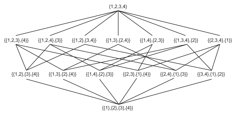
Figure 5. Merger game graph with four players.

The preceding discussions naturally lead to the question of how to evaluate the value function (7.2), which represents an infinite sum of all possible paths between states. As the graph gets more complicated, this can quickly become intractable; for example, the merger game graph becomes extremely complex as $N$ grows.

The second major contribution of this paper is to reveal the relationship between the value function and the Poisson’s equation on graphs with Hodge differential structure, when the transition probability represents a reversible Markov chain.

To describe, let $\ell^{2}({\cal V})$ be the space of functions ${\cal V}\rightarrow\mathbb{R}$ with the inner product

(7.3) $$\langle u,v\rangle\coloneqq\sum_{S\in{\cal V}}u(S)v(S).$$

Let $\lambda:\overline{{\cal E}}\to{\mathbb{R}}_{+}$ define the edge weight, satisfying $\lambda(T,S)=\lambda(S,T)\geq 0$ (i.e., no sign alternation) for all $S,T\in{\cal V}$. We declare that there is an edge between $S$ and $T$, i.e., $(S,T)\in\overline{{\cal E}}$, if and only if $\lambda(S,T)>0$. Given an edge weight $\lambda$, we denote by $\ell^{2}_{\lambda}({\cal E})$ the space of functions $\overline{{\cal E}}\rightarrow\mathbb{R}$ equipped with the weighted inner product

(7.4) $$\langle f,g\rangle_{\lambda}\coloneqq\sum_{(S,T)\in{\cal E}}\lambda(S,T)f(S,T)g(S,T)$$

with the alternating property $f(T,S)=-f(S,T)$. We then consider the operators $\mathrm{d}$ and its adjoint $\mathrm{d}^{*}$ as before: the gradient $\mathrm{d}\colon\ell^{2}({\cal V})\rightarrow\ell_{\lambda}^{2}({\cal E})$ is given by

(7.5) $$\mathrm{d}v(S,T)\coloneqq v(T)-v(S)$$

with its adjoint $\mathrm{d}^{*}\colon\ell^{2}({\cal E})\rightarrow\ell_{\lambda}^{2}({\cal V})$, the divergence, now given by

(7.6) $$\mathrm{d}^{*}f(S)=\sum_{T\sim S}\lambda(T,S)f(T,S)$$

where $T\sim S$ denotes $\lambda(S,T)>0$, i.e., $S$ and $T$ are adjacent. The Laplacian is then defined by the operator $\mathrm{d}^{\ast}\mathrm{d}:\ell^{2}({\cal V})\to\ell^{2}({\cal V})$.

We now consider the Markov chain whose transition probability has the form

(7.7) $$p_{S,T}=\frac{\lambda(S,T)}{\sum_{U\sim S}\lambda(S,U)}.$$

(7.7) represents a random walk on the graph. This includes the previous coalition process (4.1) as a special case, for which $\lambda\equiv 1$ and ${\cal G}$ is the coalition graph (3.1).

The Markov chain (7.7) is known to be time-reversible, which means that there exists a stationary distribution $\pi=(\pi_{S})_{S\in{\cal V}}$, satisfying $\pi_{S}p_{S,T}=\pi_{T}p_{T,S}$ for all $S,T\in{\cal V}$. One important implication of reversibility is that every loop and its inverse loop have the same probability of being realized, that is (see Ross [26])

(7.8) $$p_{S,S_{1}}p_{S_{1},S_{2}}\dots p_{S_{n-1},S_{n}}p_{S_{n},S}=p_{S,S_{n}}p_{S_{n},S_{n-1}}\dots p_{S_{2},S_{1}}p_{S_{1},S},$$

which property turns out to be crucial for us to establish the following result.

Theorem 7.3.

Let $f\in\ell^{2}_{\lambda}({\cal E})$ and let the Markov chain (7.7) be defined on a weighted connected graph $(G,\lambda)$. Then $V^{S}_{f}$ uniquely solves the Poisson’s equation

(7.9) $$\mathrm{d}^{*}\mathrm{d}V^{S}_{f}=\mathrm{d}^{*}f\quad\text{with}\quad V^{S}_{f}(S)=0.$$

Notice the theorem includes Proposition 4.2 and the identity 5.4 as special cases, and allows us to evaluate the potentially intractable value function $V^{S}_{f}$ by solving a tractable problem of solving a system of least-squares linear equations (7.9). In light of this, we shall call $V_{f}^{S}(\cdot)$ and its defining equation (7.9) Hodge allocation, which, in view of Proposition 5.1, can be thought of as a generalization of the Shapley formula into general cooperative network. We conclude this section by emphasizing the distinction: The initial state in the Shapley formula is always assumed to be $\emptyset$ (no one in the coalition), with the grand coalition $[N]$ always being the terminal state. In our framework, however, any two states $S,T$ on any arbitrary graph can serve as the initial and terminal states of a cooperative process.

8. Further generalization: multigraphs as cooperative networks

In this final section, we will look at how we can generalize our previous discussion for multigraphs, which can describe more general cooperative networks.

In graph theory, a multigraph is a graph that allows for multiple edges (also known as parallel edges), that is, edges with the same end nodes. As a result, two vertices can be linked by more than one edge. We assume that edges have their own identity, implying that edges, like nodes, are primitive entities. When multiple edges connect two nodes, they are considered separate edges.

The motivation for using multigraphs to describe a cooperative network is clear: even if a cooperative state $S$ is transitioned to $T$, each agent’s marginal contribution can vary depending on which route, i.e., edge, is taken for the transition. Each edge now represents a different project transition process, and the marginal contribution of agent $i$ can now be assessed differently for each edge. This also explains why we allow the graph to have loops: even if all employees work hard to make progress, it is possible that no progress is made and the project remains in the same state. Even in this case, the manager is still obligated to pay the employees’ wages.

Our final goal is to extend Theorem 7.3 into this context, thereby defining the Hodge allocation for multigraphs. Let $\kappa:{\cal V}\times{\cal V}\to{\mathbb{N}}\cup\{0\}$ represent the number of edges between two states, satisfying the symmetry $\kappa(S,T)=\kappa(T,S)$. $\kappa(S):=\kappa(S,S)$ counts the number of loops at $S$. Then for each $S,T\in{\cal V}$ (where $S=T$ is possible), let $e_{S,T}^{k,+}\in{\cal E}$ represent the $k$th forward-edge between $S$ and $T$, with its reverse $e_{S,T}^{k,-}\in{\cal E}_{-}$. Set $\overline{{\cal E}}={\cal E}\cup{\cal E}_{-}$. For an oriented edge $e\in\overline{{\cal E}}$, let $I(e)$, $J(e)$ be its initial and terminal state. Then we have $I(e_{S,T}^{k,+})=J(e_{S,T}^{k,-})$ and $I(e_{S,T}^{k,-})=J(e_{S,T}^{k,+})$.

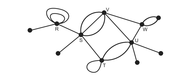
Figure 6. Multiple edges can exist between nodes in a multigraph.

Let $\ell^{2}({\cal V})$ be as before, and $\lambda:\overline{{\cal E}}\to(0,\infty)$ define the edge weight with symmetry $\lambda(e_{S,T}^{k,+})=\lambda(e_{S,T}^{k,-})$. Let $\ell^{2}_{\lambda}({\cal E})$ be the space of edge flows with the inner product

(8.1) $$\langle f,g\rangle_{\lambda}\coloneqq\sum_{e\in{\cal E}}\lambda(e)f(e)g(e)$$

satisfying the alternating property $f(e_{S,T}^{k,+})=-f(e_{S,T}^{k,-})$. The gradient $\mathrm{d}\colon\ell^{2}({\cal V})\rightarrow\ell_{\lambda}^{2}({\cal E})$ can naturally be defined by

(8.2) $$\mathrm{d}v(e)\coloneqq J(e)-I(e),\quad e\in\overline{\cal E}.$$

Then its adjoint $\mathrm{d}^{*}\colon\ell^{2}({\cal E})\rightarrow\ell_{\lambda}^{2}({\cal V})$, the divergence, is given by

(8.3) $$\mathrm{d}^{\ast}f(S)=\sum_{e\in\overline{{\cal E}},\,J(e)=S}\lambda(e)f(e)=\sum_{e\in\overline{{\cal E}},\,J(e)=S,\,I(e)\neq S}\lambda(e)f(e)$$

where the second identity is because the loop edges are effectively discarded in the sum, since $J(e^{k,+}_{S,S})=J(e^{k,-}_{S,S})=S$, $\lambda(e^{k,+}_{S,S})=\lambda(e^{k,-}_{S,S})$ and $f(e^{k,+}_{S,S})=-f(e^{k,-}_{S,S})$.

On a multigraph, we can continue to define the random cooperative process, the Markov chain $(X^{U}_{n})_{n\in{\mathbb{N}}_{0}}$ on the state space ${\cal V}$ with initial state $X_{0}=U$, driven by the transition probabilities $p(e)$ for each $e\in\overline{{\cal E}}$, where $p(e)$ now represents the probability of the process proceeding from $I(e)$ to $J(e)$ via the edge $e$.

Now, the standard notation $(X_{n})_{n}$ for stochastic processes can be insufficient in this context because we are interested not only in the states we travel through, but also in the actual path, i.e., the edges we travel through. As a result, we are led to consider an $\overline{\cal E}$-valued process $(e_{n})_{n\in{\mathbb{N}}}$, where $e_{n}=e_{n}(\omega)\in\overline{{\cal E}}$ represents the edge we traverse following its orientation. Thus we have $I(e_{n+1})=J(e_{n})$, and $X_{n}:=I(e_{n+1})$ represents the usual Markov chain on ${\cal V}$. This allows us to analogously represent an agent’s total contribution along the path $\omega$ traveling from $S$ to $T$ by

(8.4) $${\cal I}_{f}^{S}(T)={\cal I}_{f}^{S}(T)(\omega):=\sum_{n=1}^{\tau_{T}(\omega)}f\big{(}e_{n}(\omega)\big{)},$$

where $f\in\ell^{2}({\cal E})$ represents the marginal value of the agent, and $\tau_{T}(\omega)$ denotes the first time the process $\big{(}X^{S}_{n}(\omega)\big{)}_{n}$ visits $T$. Finally, the value function is defined by

(8.5) $$V_{f}^{S}(T):=\int_{\Omega}{\cal I}_{f}^{S}(T)(\omega)d{\cal P}(\omega)={\mathbb{E}}[{\cal I}_{f}^{S}(T)],$$

which is the agent’s expected total contribution if the state advances from $S$ to $T$.

In order to generalize Theorem 7.3, the final property we need is the Markov chain’s reversibility. For this, we can assume the transition probability is given by

(8.6) $$p(e^{\prime})=\frac{\lambda(e^{\prime})}{\sum_{e\in\overline{{\cal E}},\,I(e)=I(e^{\prime})}\lambda(e)},\quad e^{\prime}\in\overline{\cal E}.$$

This implies that any loop and its inverse have equal probability of being realized

(8.7) $$p(e_{1})p(e_{2})\dots p(e_{n})=p(e_{n}^{-})p(e_{n-1}^{-})\dots p(e_{1}^{-})$$

whenever $J(e_{i})=I(e_{i+1})$, $i=1,...,n$ with $e_{n+1}:=e_{1}$, and $e_{i}^{-}$ denotes the reverse edge of $e_{i}$. Now we are ready to present our final generalization for Hodge allocation.

Theorem 8.1.

Theorem 7.3 continues to hold for any $f\in\ell^{2}_{\lambda}({\cal E})$ and the reversible Markov chain (8.6) defined on any weighted connected multigraph $(G,\lambda)$.

Due to this theorem, the Hodge allocation operator (8.5) can now be effectively calculated by solving the Poisson’s equation (7.9) on any cooperative multigraph if the underlying cooperative process satisfies the reversibility (8.7).

Remark 8.2 (From infinite to finite paths).

The definition of the value function $V_{f}^{S}(\cdot)$ in (8.5) involves the sum of an infinite number of path integrals from $S$ to $T$, even when the underlying graph has a finite number of nodes and edges. This is due to the fact that we allow paths to contain loops. However, if two essential conditions are met — the alternating property of edge flows $\ell^{2}_{\lambda}({\cal E})$ and reversibility (8.7) — we can effectively reduce the sum to a finite number of appropriately weighted paths with no loops. For the sake of simplicity, let us consider the standard graph discussed in Section 7, though the same remark applies to multigraphs as well.

A path $X_{0}\to X_{1}\to\dots\to X_{k}$ has no (internal) loop if $X_{0},...,X_{k}$ are all distinct, with the exception of the possibility $X_{0}=X_{k}$, i.e., the path itself can be a loop. If a graph $G=({\cal V},{\cal E})$ is finite, then there are finitely many paths with no loops for any $S,T\in{\cal V}$. Let ${\cal N}_{S,T}$ represent the collection of such no-loop paths from $S$ to $T$. For instance, in Figure 4, ${\cal N}_{S,T}$ consists of the following three paths:

$$S\to T,\ S\to V\to U\to T,\ S\to V\to W\to U\to T.$$

On the other hand, let ${\cal C}_{S,T}$ represent the collection of all paths from $S$ to $T$, that is, $X_{0}=S$, $X_{k}=T$, and $X_{i}\neq T$ for all $1\leq i\leq k-1$. We now assert:

(8.8) $$V_{f}^{S}(T)=\sum_{\tilde{\omega}=(X_{0},...,X_{k})\in{\cal N}_{S,T}}\mu(\tilde{\omega})\sum_{n=1}^{k}f(X_{n-1},X_{n})$$

for some probability $\mu$ on ${\cal N}_{S,T}$, i.e., $\sum_{\tilde{\omega}\in{\cal N}_{S,T}}\mu(\tilde{\omega})=1$ with $\mu(\tilde{\omega})>0$ for every $\tilde{\omega}$.

What probability $\mu$ will make (8.8) hold? Let us declare that $\omega\in{\cal C}_{S,T}$ and $\tilde{\omega}\in{\cal N}_{S,T}$ are equivalent, denoted by $\omega\sim\tilde{\omega}$, which means that if all internal loops in $\omega$ are removed, it equals $\tilde{\omega}$. For example, in Figure 4, the path $S\to V\to W\to U\to V\to W\to U\to T$ is equivalent to $S\to V\to W\to U\to T$. Now $\mu$ is defined by:

(8.9) $$\mu(\tilde{\omega})={\cal P}(\{\omega\ |\ \omega\sim\tilde{\omega}\})=\int_{\{\omega\,|\,\omega\sim\tilde{\omega}\}}d{\cal P}(\omega)$$

where ${\cal P}$ is the law of the Markov chain, so for $\omega=(X_{0},X_{1},...,X_{k})$, we have $d{\cal P}(\omega)=\prod_{n=1}^{k}p_{X_{n-1},X_{n}}=p_{X_{0},X_{1}}p_{X_{1},X_{2}}\dots p_{X_{k-1}X_{k}}$.

As an example, for the pure bargaining game $\delta_{[2]}$ with two players, consider initial and terminal states as $\emptyset$ and $\{1\}$. There are two no-loop paths: $\tilde{\omega}_{1}=(\emptyset,\{1\})$ and $\tilde{\omega}_{2}=(\emptyset,\{2\},\{1,2\},\{1\})$. If we assign $1/2$ to $\tilde{\omega}_{1}$ and $(1/2)^{3}=1/8$ to $\tilde{\omega}_{2}$ according to their lengths, it fails to sum to $1$, and it will not yield a proper weight assignment.

Now consider the unbiased random walk $\{X_{n}\}_{n\geq 0}$ with $X_{0}=\emptyset$. With probability $1/2$, $X_{1}=\{1\}$ or $\{2\}$. In the latter case $X_{1}=\{2\}$, due to graph symmetry, the random walk will eventually arrive at $\{1\}$ via $\emptyset$ or $\{1,2\}$ with equal probability $1/2$. Notice this tells us that $\mu(\tilde{\omega}_{1})=1/2+1/2\cdot 1/2=3/4$ and $\mu(\tilde{\omega}_{2})=1/2\cdot 1/2=1/4$. Now the path integral of $\mathrm{d}_{1}v$ along $\tilde{\omega}_{1}$ is $0$, while along $\tilde{\omega}_{2}$ is $1$, resulting in player $1$’s value at $\{1\}$ as $3/4\cdot 0+1/4\cdot 1=1/4$. Similarly, the path integral of $\mathrm{d}_{2}v$ along $\tilde{\omega}_{1}$ is $0$, while along $\tilde{\omega}_{2}$ is $-1$, yielding player $2$’s value at $\{1\}$ as $3/4\cdot 0+1/4\cdot(-1)=-1/4$. This is the component game values $v_{1}(\{1\})$ and $v_{2}(\{1\})$, verifying (8.8) in this case.

For establishing (8.8) in general, the alternating property of edge flows and the reversibility of the Markov chain will be crucial, which implies that the path integral of an edge flow along a loop and its reverse loop must have the opposite sign and thus cancel out in the sum (8.8). This observation is also important for the proof of Lemma 9.3 (which is then the key to the proofs of Theorems 7.3 and 8.1) and is discussed in detail in the following section, so we skip the proof of (8.8). If, on the other hand, at least one of the two conditions fails, the author does not expect the reduction (8.8) to hold in general. This signifies the importance of the conditions.

9. Proofs of the results

We will now present proofs. Results will be restated for the reader’s convenience.

Theorem 9.1.

There exists a unique allocation map $v\in{\cal G}\mapsto\bigl{(}\Phi_{i}[v]\bigr{)}_{i\in{\mathbb{N}}}$ satisfying $\Phi_{i}[v]\in{\cal G}_{N}$ with $\Phi_{i}[v]\equiv 0$ for $i>N$ if $v\in{\cal G}_{N}$, and also the following conditions:

A1(efficiency): $v=\sum_{i\in{\mathbb{N}}}\Phi_{i}[v]$.

A2(symmetry): $\Phi_{i}[v^{ij}](S^{ij})=\Phi_{j}[v](S)$ for all $v\in{\cal G}_{N}$, $i,j\in[N]$ and $S\subseteq[N]$.

A3(null-player): If $v\in{\cal G}_{N}$ and $\mathrm{d}_{i}v=0$ for some $i\in[N]$, then $\Phi_{i}[v]\equiv 0$, and

$$\Phi_{j}[v](S\cup\{i\})=\Phi_{j}[v](S)=\Phi_{j}[v_{-i}](S)\ \text{ for all }\ j\in[N]\setminus\{i\},\,S\subseteq[N]\setminus\{i\}.$$

A4(linearity): For any $v,v^{\prime}\in{\cal G}_{N}$ and $\alpha,\alpha^{\prime}\in{\mathbb{R}}$, $\Phi_{i}[\alpha v+\alpha^{\prime}v^{\prime}]=\alpha\Phi_{i}[v]+\alpha^{\prime}\Phi_{i}[v^{\prime}]$.

A5(reflection): For any $v\in{\cal G}_{N}$ and $S\subseteq[N]\setminus\{i,j\}$ with $i\neq j$, it holds

$$\Phi_{i}[v](S\cup\{i,j\})-\Phi_{i}[v](S\cup\{i\})=\Phi_{i}[v](S)-\Phi_{i}[v](S\cup\{j\}).$$

Furthermore, the solution $v_{i}\in{\cal G}_{N}$ to (3.10) satisfy A1–A5 with the identification $\Phi_{i}[v]=v_{i}$. In other words, A1–A5 characterizes the solutions $\{v_{i}\}_{i\in[N]}$ to (3.10).

Proof.

Recall that A5 is equivalent to A5’, i.e., for any $S,T\subseteq[N]\setminus\{i\}$, it holds

(9.1) $$\Phi_{i}[v](S\cup\{i\})-\Phi_{i}[v](T\cup\{i\})=-\bigl{(}\Phi_{i}[v](S)-\Phi_{i}[v](T)\bigr{)}.$$

We claim that A1–A5’ determines the linear operator $\Phi$ uniquely (if exists). For each $N\in{\mathbb{N}}$, define the basis games $\delta_{S,N}$ of ${\cal G}_{N}$ for every $S\subseteq[N]$, $S\neq\emptyset$, by

$$\delta_{S,N}(S)=1,\quad\delta_{S,N}(T)=0\,\text{ if }\,T\neq S.$$

We proceed by an induction on $N$. The case $N=1$ is already from A1. Suppose the claim holds for $N-1$, so $\Phi_{i}[\delta_{S,N-1}]$ are determined for all $S\in 2^{[N-1]}\setminus\{\emptyset\}$. Now define the games $\Delta_{(S,S\cup\{i\})}\in{\cal G}_{N}$ for each $i\in[N]$, $S\subseteq[N]\setminus\{i\}$, $S\neq\emptyset$, by

$$\Delta_{(S,S\cup\{i\})}(T)=1\,\text{ if }\,T=S\text{ or }T=S\cup\{i\},\quad\Delta_{(S,S\cup\{i\})}(T)=0\,\text{ otherwise.}$$

Notice then A3 (and induction hypothesis) determines $\Phi$ for all $\Delta_{(S,S\cup\{i\})}\in{\cal G}_{N}$. Then thanks to A4, to prove the claim, it is enough to show that A1–A5’ can determine $\Phi$ for the pure bargaining game $\delta:=\delta_{[N],N}$, because for any $S\subseteq[N]$, we can write $\delta_{S,N}$ as the following sign-alternating sum

$$\delta_{S,N}=\Delta_{(S,S\cup\{i_{1}\})}-\Delta_{(S\cup\{i_{1}\},S\cup\{i_{1},i_{2}\})}+\Delta_{(S\cup\{i_{1},i_{2}\},S\cup\{i_{1},i_{2},i_{3}\})}-\dots\pm\delta_{[N],N}.$$

By A2, $\sum_{S\subseteq[N]}\Phi_{i}[\delta](S)$ is constant for all $i\in[N]$, thus equals $1/N$ by A1. Define

$$u_{i}(S):=\Phi_{i}[\delta](S)-\frac{1}{N2^{N}}\ \text{ for all }\ S\subseteq[N]$$

so that $u_{i}(\emptyset)=-\frac{1}{N2^{N}}$ and $\sum_{S\subseteq[N]}u_{i}(S)=0$ for all $i$. Now observe A5’ implies:

$$u_{i}(S)+u_{i}(S\cup\{i\})\text{ is constant for all }S\subseteq[N]\setminus\{i\},\text{ hence it is zero.}$$

This determines $u_{i}$ thus $\Phi_{i}[\delta]$ as follows: suppose $u_{i}(S)$ has been determined for all $i$ and $|S|\leq k-1$. Let $|T|=k\leq N-1$. Then we have $u_{i}(T)=-u_{i}(T\setminus\{i\})$ for all $i\in T$ and it is constant (say $c_{k}$) by A2. Using A1 and A2, we then observe

$$0=\delta(T)=\sum_{i\in[N]}\Phi_{i}[\delta](T)=\sum_{i\in[N]}\bigg{(}u_{i}(T)+\frac{1}{N2^{N}}\bigg{)},$$

yielding $\sum_{i\in[N]}u_{i}(T)=-1/2^{N}$. With $u_{i}(T)=c_{k}$ for all $i\in T$, we deduce that $u_{j}(T)=\frac{-1-2^{N}kc_{k}}{2^{N}(N-k)}$ for all $j\notin T$. Of course, $\Phi_{i}[\delta]([N])=1/N$ for all $i\in[N]$ by A1 and A2. By induction (on $N$ and on $k$ for each $N$), the proof of uniqueness of the operator $\Phi$ is therefore complete.

It remains to show the solutions $(v_{i})_{i\in[N]}$ to (3.10) satisfy A1–A5’ with $\Phi_{i}[v]=v_{i}$. Firstly, A4 is clearly satisfied by $(v_{i})_{i}$. To show that A1 is satisfied, we compute

$$\mathrm{d}^{\ast}\mathrm{d}\sum_{i\in[N]}v_{i}=\sum_{i\in[N]}\mathrm{d}^{\ast}\mathrm{d}v_{i}=\sum_{i\in[N]}\mathrm{d}^{\ast}\mathrm{d}_{i}v=\mathrm{d}^{\ast}\sum_{i\in[N]}\mathrm{d}_{i}v=\mathrm{d}^{\ast}\mathrm{d}v,$$

since $\mathrm{d}=\sum_{i\in[N]}\mathrm{d}_{i}$. Hence by unique solvability of (3.10), $\sum_{i\in[N]}v_{i}=v$ as desired. Next let $\sigma$ be a permutation of $[N]$. As in [31], let $\sigma$ act on $\ell^{2}(2^{[N]})$ and $\ell^{2}({\cal E})$ via

$$\sigma v(S)=v(\sigma(S))\ \text{and}\ \sigma f\bigl{(}S,S\cup\{i\}\bigr{)}=f\bigl{(}\sigma(S),\sigma(S\cup\{i\})\bigr{)},\ v\in\ell^{2}(2^{[N]}),\ f\in\ell^{2}({\cal E}).$$

It is easy to check $\mathrm{d}\sigma=\sigma\mathrm{d}$ and $\mathrm{d}_{i}\sigma=\sigma\mathrm{d}_{\sigma(i)}$. We also have $\mathrm{d}^{\ast}\sigma=\sigma\mathrm{d}^{\ast}$, since

$$\langle v,\mathrm{d}^{\ast}\sigma f\rangle=\langle\mathrm{d}v,\sigma f\rangle=\langle\sigma^{-1}\mathrm{d}v,f\rangle=\langle\mathrm{d}\sigma^{-1}v,f\rangle=\langle\sigma^{-1}v,\mathrm{d}^{\ast}f\rangle=\langle v,\sigma\mathrm{d}^{\ast}f\rangle$$

for any $v\in\ell^{2}(2^{[N]})$, $f\in\ell^{2}({\cal E})$. Now let $\sigma$ be the transposition of $i,j$. We have

$$\mathrm{d}^{\ast}\mathrm{d}(\sigma v)_{i}=\mathrm{d}^{\ast}\mathrm{d}_{i}\sigma v=\mathrm{d}^{\ast}\sigma\mathrm{d}_{j}v=\sigma\mathrm{d}^{\ast}\mathrm{d}_{j}v=\sigma\mathrm{d}^{\ast}\mathrm{d}v_{j}=\mathrm{d}^{\ast}\mathrm{d}\sigma v_{j}$$

which shows $(\sigma v)_{i}=\sigma v_{j}$ by the unique solvability. Notice this corresponds to A2.

For A3, let $v\in{\cal G}_{N}$, $i\in[N]$, and assume $\mathrm{d}_{i}v=0$. Then from (3.10) we readily get $v_{i}\equiv 0$. Fix $j\neq i$, and let $\mathrm{\tilde{d}}$, $\mathrm{\tilde{d}}_{j}$ be the differential operators restricted on $2^{[N]\setminus\{i\}}$, and set $\tilde{v}=v_{-i}$, i.e., $\tilde{v}$ is the restriction of $v$ on $2^{[N]\setminus\{i\}}$. Let $\tilde{v}_{j}$ be the corresponding component game on $2^{[N]\setminus\{i\}}$, solving the defining equation $\mathrm{\tilde{d}}^{\ast}\mathrm{\tilde{d}}\tilde{v}_{j}=\mathrm{\tilde{d}}^{\ast}\mathrm{\tilde{d}}_{j}\tilde{v}$. Finally, in view of A3, define $v_{j}\in{\cal G}_{N}$ by $v_{j}=\tilde{v}_{j}$ on $2^{[N]\setminus\{i\}}$ and $\mathrm{d}_{i}v_{j}=0$. Now observe that A3 will follow if we can verify that this $v_{j}$ indeed solves the equation $\mathrm{d}^{\ast}\mathrm{d}v_{j}=\mathrm{d}^{\ast}\mathrm{d}_{j}v$.

To show this, let $S\subseteq[N]\setminus\{i\}$. In fact the following string of equalities holds:

$$\mathrm{d}^{\ast}\mathrm{d}v_{j}(S\cup\{i\})=\mathrm{d}^{\ast}\mathrm{d}v_{j}(S)=\mathrm{\tilde{d}}^{\ast}\mathrm{\tilde{d}}\tilde{v}_{j}(S)=\mathrm{\tilde{d}}^{\ast}\mathrm{\tilde{d}}_{j}\tilde{v}(S)=\mathrm{d}^{\ast}\mathrm{d}_{j}v(S)=\mathrm{d}^{\ast}\mathrm{d}_{j}v(S\cup\{i\})$$

which simply follows from the definition of the differential operators. For instance

$$\mathrm{d}^{\ast}\mathrm{d}v_{j}(S)=\sum_{T\sim S}\mathrm{d}v_{j}(T,S)=\sum_{T\sim S,\,T\neq S\cup\{i\}}\mathrm{d}v_{j}(T,S)=\mathrm{\tilde{d}}^{\ast}\mathrm{\tilde{d}}\tilde{v}_{j}(S)$$

where the second equality is due to $\mathrm{d}_{i}v_{j}=0$. On the other hand, since $j\neq i$,

$$\mathrm{d}^{\ast}\mathrm{d}_{j}v(S)=\sum_{T\sim S}\mathrm{d}_{j}v(T,S)=\sum_{T\sim S}\mathrm{\tilde{d}}_{j}\tilde{v}(T,S)=\mathrm{\tilde{d}}^{\ast}\mathrm{\tilde{d}}_{j}\tilde{v}(S).$$

The first and last equalities in the string should now be obvious, verifying A3.

Finally, we verify A5’. For this, we need to verify the following claim:

(9.2) $$v_{i}(S)+v_{i}(S\cup\{i\})\,\text{ is constant over all }\,S\subseteq[N]\setminus\{i\}.$$

Let $S\subseteq[N]\setminus\{i\}$, and recall $\mathrm{d}^{\ast}\mathrm{d}_{i}v(S)=v(S)-v(S\cup\{i\})=-\mathrm{d}^{\ast}\mathrm{d}_{i}v(S\cup\{i\})$. Hence $\mathrm{d}^{\ast}\mathrm{d}v_{i}(S)+\mathrm{d}^{\ast}\mathrm{d}v_{i}(S\cup\{i\})=0$. Define $w_{i}\in\ell^{2}(2^{[N]})$ by $w_{i}(S)=v_{i}(S\cup\{i\})$ and $w_{i}(S\cup\{i\})=v_{i}(S)$ for all $S\subseteq[N]\setminus\{i\}$. Then clearly $\mathrm{d}^{\ast}\mathrm{d}v_{i}(S\cup\{i\})=\mathrm{d}^{\ast}\mathrm{d}w_{i}(S)$ and $\mathrm{d}^{\ast}\mathrm{d}v_{i}(S)=\mathrm{d}^{\ast}\mathrm{d}w_{i}(S\cup\{i\})$. Thus $\mathrm{d}^{\ast}\mathrm{d}(v_{i}+w_{i})\equiv 0$, hence $v_{i}+w_{i}\in\mathcal{N}(\mathrm{d})$, meaning that $v_{i}+w_{i}$ is constant. This proves the claim, hence the theorem. ∎

We then prove Proposition 5.1, the coincidence between the $f$-Shapley value $\phi_{f}$ and $v_{f}([N])$, the grand coalition value of the solution of the equation $\mathrm{d}^{\ast}\mathrm{d}v_{f}=\mathrm{d}^{\ast}f$. The proof is already alluded to in a remark in [31], which we will follow here.

Proposition 9.2.

$\phi_{f}=v_{f}([N])$  for any edge flow $f$ on the coalition game graph.

Proof.

Observe first that the map $f\in\ell^{2}({\cal E})\mapsto\phi_{f}$ is linear. By linearity, notice it is enough to prove the proposition when $f=\chi_{(S,S\cup\{i\})}\in\ell^{2}({\cal E})$, which is the indicator function equal to $1$ on $\bigl{(}S,S\cup\{i\}\bigr{)}$ and $0$ on all other edges of (3.1).

Let $k=\lvert S\rvert\in\{0,1,...,N-1\}$. For this $f$, the $f$-Shapley formula (5.2) yields

(9.3) $$\phi_{f}=\frac{k!(N-1-k)!}{N!}.$$

Next, following [31], we consider $v\in{\cal G}_{N}$ defined by

$$v(T)\coloneqq 1\,\text{ if }\,\lvert T\rvert>k,\quad 0\,\text{ if }\,\lvert T\rvert\leq k,$$

so that

$$\mathrm{d}v=\sum_{\begin{subarray}{c}\lvert T\rvert=k\\ j\notin T\end{subarray}}\chi_{(T,T\cup\{j\})}.$$

Let $v_{(T,T\cup\{j\})}$ solve $\mathrm{d}^{\ast}\mathrm{d}v_{(T,T\cup\{j\})}=\mathrm{d}^{\ast}\chi_{(T,T\cup\{j\})}$ with $v_{(T,T\cup\{j\})}(\emptyset)=0$. Then we have

$$\mathrm{d}^{\ast}\mathrm{d}v=\sum_{\begin{subarray}{c}\lvert T\rvert=k\\ j\notin T\end{subarray}}\mathrm{d}^{\ast}\chi_{(T,T\cup\{j\})}=\sum_{\begin{subarray}{c}\lvert T\rvert=k\\ j\notin T\end{subarray}}\mathrm{d}^{\ast}\mathrm{d}v_{(T,T\cup\{j\})}=\mathrm{d}^{\ast}\mathrm{d}\sum_{\begin{subarray}{c}\lvert T\rvert=k\\ j\notin T\end{subarray}}v_{(T,T\cup\{j\})},$$

yielding $\displaystyle\sum_{\lvert T\rvert=k,\,j\notin T}v_{(T,T\cup\{j\})}=v$, hence $\displaystyle\sum_{\lvert T\rvert=k,\,j\notin T}v_{(T,T\cup\{j\})}([N])=v([N])=1$.

This sum contains $\binom{N}{k}\bigl{(}N-k\bigr{)}=\frac{N!}{k!(N-1-k)!}$ terms, and the symmetry of the hypercube (3.1) implies that all of the terms $v_{(T,T\cup\{j\})}([N])$ in the sum is a constant, so it equals $v_{f}([N])$. This yields $v_{f}([N])=\phi_{f}$ as desired. ∎

Now we’ll look at the proof of Theorem 7.3. This necessitates the development of a transition formula for the value function. The fact that the Markov chain is irreducible and thus visits every state infinitely many times is used implicitly.

Lemma 9.3.

Let $(G,\lambda)$ be any weighted connected graph. For any $S,T,U\in{\cal V}$ and $f\in\ell^{2}_{\lambda}({\cal E})$, we have $V^{U}_{f}(T)-V^{U}_{f}(S)=V_{f}^{S}(T)$. In particular, $V_{f}^{S}(T)=-V_{f}^{T}(S)$, and $V_{f}^{S}(S)=0$.

Proof.

We firstly show $V_{f}^{S}(S)=0$ which appears as the initial condition in (7.9). Then we show $V_{f}^{S}(T)=-V_{f}^{T}(S)$. Finally, we show $V^{U}_{f}(T)-V^{U}_{f}(S)=V_{f}^{S}(T)$.

To see $V_{f}^{S}(S)=0$, consider a general sample path $\omega$ starting and ending at $S$, without visiting $S$ along the way. In other words, $\omega$ is a loop emanating from $S$. Let $\omega^{-1}$ denote the reversed path of $\omega$, that is, if $\omega$ visits $T_{0}\to T_{1}\to\dots\to T_{k}$ (where $T_{0}=T_{k}=S$ if $\omega$ is a loop), then $\omega^{-1}$ visits $T_{k}\to\dots\to T_{0}$. Observe

$$0 ={\cal I}_{f}^{S}(S)(\omega)-{\cal I}_{f}^{S}(S)(\omega)$$

$$=\sum_{n=1}^{\tau_{S}(\omega)}f\big{(}X^{S}_{n-1}(\omega),X^{S}_{n}(\omega)\big{)}-\sum_{n=1}^{\tau_{S}(\omega)}f\big{(}X^{S}_{n-1}(\omega),X^{S}_{n}(\omega)\big{)}$$

$$=\sum_{n=1}^{\tau_{S}(\omega)}f\big{(}X^{S}_{n-1}(\omega),X^{S}_{n}(\omega)\big{)}+\sum_{n=1}^{\tau_{S}(\omega)}f\big{(}X^{S}_{n}(\omega),X^{S}_{n-1}(\omega)\big{)}$$

$$=\sum_{n=1}^{\tau_{S}(\omega)}f\big{(}X^{S}_{n-1}(\omega),X^{S}_{n}(\omega)\big{)}+\sum_{n=1}^{\tau_{S}(\omega^{-1})}f\big{(}X^{S}_{n-1}(\omega^{-1}),X^{S}_{n}(\omega^{-1})\big{)}.$$

Let ${\cal P}(\omega)$ denote the probability of the sample path $\omega$ being realized, that is, ${\cal P}(\omega)=p_{T_{0},T_{1}}p_{T_{1},T_{2}}\dots p_{T_{k-1},T_{k}}$. Now observe that the time-reversibility (7.8) implies ${\cal P}(\omega)={\cal P}(\omega^{-1})$ for a loop $\omega$. And there is an obvious one-to-one correspondence between a loop $\omega$ and its reverse $\omega^{-1}$. This implies

$$0 =\int_{\omega}\sum_{n=1}^{\tau_{S}(\omega)}f\big{(}X^{S}_{n-1}(\omega),X^{S}_{n}(\omega)\big{)}d{\cal P}(\omega)+\int_{\omega}\sum_{n=1}^{\tau_{S}(\omega^{-1})}f\big{(}X^{S}_{n-1}(\omega^{-1}),X^{S}_{n}(\omega^{-1})\big{)}d{\cal P}(\omega)$$

$$=\int_{\omega}\sum_{n=1}^{\tau_{S}(\omega)}f\big{(}X^{S}_{n-1}(\omega),X^{S}_{n}(\omega)\big{)}d{\cal P}(\omega)+\int_{\omega}\sum_{n=1}^{\tau_{S}(\omega^{-1})}f\big{(}X^{S}_{n-1}(\omega^{-1}),X^{S}_{n}(\omega^{-1})\big{)}d{\cal P}(\omega^{-1})$$

$$=V_{f}^{S}(S)+V_{f}^{S}(S)$$

yielding $V_{f}^{S}(S)=0$ as desired.

Next, we will show $V_{f}^{S}(T)=-V_{f}^{T}(S)$ for $S\neq T$. Consider a general finite sample path $\omega$ of the Markov chain (4.1) starting at $S$, visiting $T$, then returning to $S$ (this happens with probability 1). We can split this journey into four subpaths: $\omega_{1}$: the path returns to $S$ $m\in{\mathbb{N}}\cup\{0\}$ times without visiting $T$, $\omega_{2}$: the path begins at $S$ and ends at $T$ without returning to $S$, $\omega_{3}$: the path returns to $T$ $n\in{\mathbb{N}}\cup\{0\}$ times without visiting $S$, $\omega_{4}$: the path begins at $T$ and ends at $S$ without returning to $T$.

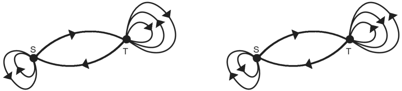
Figure 7. $\omega=\omega_{1}\circ\omega_{2}\circ\omega_{3}\circ\omega_{4}$ and its pair $\omega^{\prime}=\omega^{-1}_{1}\circ\omega_{2}\circ\omega_{3}^{-1}\circ\omega_{4}$. By reversibility, they have the same probability of being realized.

Thus $\omega=\omega_{1}\circ\omega_{2}\circ\omega_{3}\circ\omega_{4}$ is the concatenation of the $\omega_{i}$’s, and the probability ${\cal P}(\omega)$ of this finite sample path being realized satisfies ${\cal P}(\omega)={\cal P}(\omega_{1}){\cal P}(\omega_{2}){\cal P}(\omega_{3}){\cal P}(\omega_{4})$.

Define a pairing $\omega^{\prime}$ of $\omega$ by $\omega^{\prime}:=\omega^{-1}_{1}\circ\omega_{2}\circ\omega_{3}^{-1}\circ\omega_{4}$. This is another general sample path starting at $S$, visiting $T$, then returning to $S$. Then we have ${\cal P}(\omega)={\cal P}(\omega^{\prime})$ because ${\cal P}(\omega_{1})={\cal P}(\omega^{-1}_{1})$ and ${\cal P}(\omega_{3})={\cal P}(\omega^{-1}_{3})$ by (7.8), and moreover,

$${\cal I}_{f}^{S}(T)(\omega)+{\cal I}_{f}^{S}(T)(\omega^{\prime})=2\sum_{n=1}^{\tau_{T}(\omega_{2})}f\big{(}X^{S}_{n-1}(\omega_{2}),X^{S}_{n}(\omega_{2})\big{)},$$

because the loops $\omega_{1}$ and $\omega^{-1}_{1}$ aggregate $f$ with opposite signs, hence they cancel out in the above sum. Now consider $\tilde{\omega}:=\omega_{3}\circ\omega_{2}^{-1}\circ\omega_{1}\circ\omega_{4}^{-1}$ and $\tilde{\omega}^{\prime}:=\omega_{3}^{-1}\circ\omega_{2}^{-1}\circ\omega_{1}^{-1}\circ\omega_{4}^{-1}$. $(\tilde{\omega},\tilde{\omega}^{\prime})$ then represents a pair of general sample paths starting at $T$, visiting $S$, then returning to $T$. We then deduce

$${\cal I}_{f}^{T}(S)(\tilde{\omega})+{\cal I}_{f}^{T}(S)(\tilde{\omega}^{\prime}) =2\sum_{n=1}^{\tau_{S}(\omega_{2}^{-1})}f\big{(}X^{T}_{n-1}(\omega_{2}^{-1}),X^{T}_{n}(\omega_{2}^{-1})\big{)}$$

$$=-2\sum_{n=1}^{\tau_{T}(\omega_{2})}f\big{(}X^{S}_{n-1}(\omega_{2}),X^{S}_{n}(\omega_{2})\big{)}$$

$$=-\big{(}{\cal I}_{f}^{S}(T)(\omega)+{\cal I}_{f}^{S}(T)(\omega^{\prime})\big{)}$$

because $f(U,V)=-f(V,U)$ for any edge $(U,V)$. Due to the one-to-one correspondence between the paths $\omega,\omega^{\prime},\tilde{\omega},\tilde{\omega}^{\prime}$, and ${\cal P}(\omega)={\cal P}(\omega^{\prime})={\cal P}(\tilde{\omega})={\cal P}(\tilde{\omega}^{\prime})$ from (7.8), the desired identity $V_{f}^{S}(T)=-V_{f}^{T}(S)$ now follows by integration:

$$\int_{\omega}\big{[}{\cal I}_{f}^{T}(S)(\tilde{\omega})+{\cal I}_{f}^{T}(S)(\tilde{\omega}^{\prime})\big{]}d{\cal P}(\omega) =\int_{\omega}{\cal I}_{f}^{T}(S)(\tilde{\omega})d{\cal P}(\tilde{\omega})+\int_{\omega}{\cal I}_{f}^{T}(S)(\tilde{\omega}^{\prime})d{\cal P}(\tilde{\omega}^{\prime})$$

$$=2V_{f}^{T}(S),$$

and similarly,

$$\int_{\omega}\big{[}{\cal I}_{f}^{S}(T)(\omega)+{\cal I}_{f}^{S}(T)(\omega^{\prime})\big{]}d{\cal P}(\omega)=2V_{f}^{S}(T).$$

Finally, to show $V_{f}^{U}(T)-V_{f}^{U}(S)=V^{S}_{f}(T)$ for distinct $S,T,U$, we proceed

$${\cal I}_{f}^{U}(T)-{\cal I}_{f}^{U}(S)=\sum_{n=1}^{\tau_{T}}f\big{(}X^{U}_{n-1},X^{U}_{n}\big{)}-\sum_{n=1}^{\tau_{S}}f\big{(}X^{U}_{n-1},X^{U}_{n}\big{)}$$

$$={\bf 1}_{\tau_{S}<\tau_{T}}\sum_{n=\tau_{S}+1}^{\tau_{T}}f\big{(}X^{U}_{n-1},X^{U}_{n}\big{)}-{\bf 1}_{\tau_{T}<\tau_{S}}\sum_{n=\tau_{T}+1}^{\tau_{S}}f\big{(}X^{U}_{n-1},X^{U}_{n}\big{)}.$$

By taking expectation, we obtain the following via the Markov property

$${\mathbb{E}}[{\cal I}_{f}^{U}(T)]-{\mathbb{E}}[{\cal I}_{f}^{U}(S)] ={\cal P}(\{\tau_{S}<\tau_{T}\})V^{S}_{f}(T)-{\cal P}(\{\tau_{T}<\tau_{S}\})V^{T}_{f}(S)$$

$$=\big{(}{\cal P}(\{\tau_{S}<\tau_{T}\})V^{S}_{f}(T)+{\cal P}(\{\tau_{T}<\tau_{S}\})\big{)}V^{S}_{f}(T)$$

$$=V^{S}_{f}(T)$$

which proves the transition formula $V_{f}^{U}(T)-V_{f}^{U}(S)=V^{S}_{f}(T)$. ∎

Theorem 9.4.

Let $f\in\ell^{2}_{\lambda}({\cal E})$ and let the Markov chain (7.7) be defined on a weighted connected graph $(G,\lambda)$. Then $V^{S}_{f}$ uniquely solves the Poisson’s equation

(9.4) $$\mathrm{d}^{*}\mathrm{d}V^{S}_{f}=\mathrm{d}^{*}f\quad\text{with}\quad V^{S}_{f}(S)=0.$$

Proof.

$V^{S}_{f}(S)=0$ was shown in Lemma 9.3. Connectedness of $G$ implies that the nullspace $\cal N(\mathrm{d})$ is one-dimensional, spanned by the constant function $1$ on ${\cal V}$. Now if $\mathrm{d}^{\ast}\mathrm{d}u=\mathrm{d}^{\ast}\mathrm{d}v$, then we have $u-v\in\cal N(\mathrm{d})$. This yields the uniqueness of the solution $V^{S}_{f}$ satisfying the initial condition $V^{S}_{f}(S)=0$.

Fix $T\in{\cal V}$, and let $\{T_{1},...,T_{n}\}$ be the set of all states adjacent to $T$ (i.e., either $(T,T_{k})$ or $(T_{k},T)$ is in ${\cal E}$), and set $\Lambda_{T}=\sum_{k=1}^{n}\lambda(T,T_{k})$. By (7.6), (7.7), we have

(9.5) $$\mathrm{d}^{*}f(T)/\Lambda_{T} =\sum_{k=1}^{n}p_{T,T_{k}}f(T_{k},T),\text{ and}$$

(9.6) $$\mathrm{d}^{*}\mathrm{d}V^{S}_{f}(T)/\Lambda_{T} =\sum_{k=1}^{n}p_{T,T_{k}}\big{(}V^{S}_{f}(T)-V^{S}_{f}(T_{k})\big{)}=\sum_{k=1}^{n}p_{T,T_{k}}V_{f}^{T_{k}}(T)$$

where the last equality is from Lemma 9.3. Now we can interpret the right side of (9.6) as the aggregation (7.2) of path integrals of $f$ (7.1) along all loops beginning and ending at $T$, but in this aggregation of $f$ we do not take into account the first move from $T$ to $T_{k}$, since this first move is described by the transition rate $p_{T,T_{k}}$ and not driven by $V^{T_{k}}_{f}$. On the other hand, if we aggregate path integrals of $f$ for all loops emanating from $T$, we get $0$ due to the reversibility (7.8) and alternating property of $f$, that is, $V_{f}^{T}(T)=0$. This observation allows us to conclude as follows:

$$0 =\text{aggregation of path integrals of $f$ along all loops emanating from $T$}$$

$$=\text{aggregation of path integrals of $f$ along all loops except the first moves}$$

$$\quad+\text{aggregation of path integrals of $f$ for all first moves from $T$}$$

$$=\sum_{k=1}^{n}p_{T,T_{k}}V_{f}^{T_{k}}(T)+\sum_{k=1}^{n}p_{T,T_{k}}f(T,T_{k})$$

$$=\mathrm{d}^{*}\mathrm{d}V^{S}_{f}(T)/\Lambda_{T}-\mathrm{d}^{*}f(T)/\Lambda_{T},$$

yielding $\mathrm{d}^{*}\mathrm{d}V^{S}_{f}(T)=\mathrm{d}^{*}f(T)$, as desired. ∎

Finally, we prove the following extension of the previous theorem for multigraphs.

Theorem 9.5.

Theorem 7.3 continues to hold for any $f\in\ell^{2}_{\lambda}({\cal E})$ and the reversible Markov chain (8.6) defined on any weighted connected multigraph $(G,\lambda)$.

Proof.

We’ve seen that the most crucial we need is the reversibility (8.7). Recall we now consider an $\overline{\cal E}$-valued process $(e_{n})$, $n\in{\mathbb{N}}$, where $e_{n}=e_{n}(\omega)\in\overline{{\cal E}}$ represents the edge we traverse following its orientation, whose transition rate is given by

(9.7) $$p(e^{\prime})=\frac{\lambda(e^{\prime})}{\sum_{e\in\overline{{\cal E}},\,I(e)=I(e^{\prime})}\lambda(e)},$$

and $X_{n}=I(e_{n+1})$ represents the standard Markov chain on ${\cal V}$. What is the transition rate $(p_{S,T})_{(S,T)\in{\cal V}\times{\cal V}}$ of $X_{n}$? (Note $S=T$ is possible) Notice (9.7) gives:

(9.8) $$p_{S,T}=\frac{\sum_{e\in\overline{{\cal E}},\,I(e)=S,\,J(e)=T}\lambda(e)}{\sum_{e\in\overline{{\cal E}},\,I(e)=S}\lambda(e)}=:\frac{\Lambda_{S,T}}{\Lambda_{S}}.$$

The standard theory of Markov chain now yields a stationary distribution $\pi=(\pi_{S})_{S\in{\cal V}}$, $\pi_{S}>0$ for all $S\in{\cal V}$, which satisfies

(9.9) $$\pi_{S}p_{S,T}=\pi_{T}p_{T,S}\ \text{ for all }\ S,T\in{\cal V}.$$

Let $e\in\overline{\cal E}$ have $S,T$ as its endpoints, i.e., $I(e)=S$, $J(e)=T$. Let $e^{-}$ be its reverse. Then (9.9) implies

(9.10) $$\pi_{S}p(e)=\pi_{T}p(e^{-})$$

because $\pi_{S}p(e)=\pi_{S}\frac{\lambda(e)}{\Lambda_{S}}=\pi_{S}p_{S,T}\frac{\lambda(e)}{\Lambda_{S,T}}=\pi_{T}p_{T,S}\frac{\lambda(e^{-})}{\Lambda_{T,S}}=\pi_{T}\frac{\lambda(e^{-})}{\Lambda_{T}}=\pi_{T}p(e^{-})$, using the fact $\Lambda_{S,T}=\Lambda_{T,S}$ inherited from the symmetry of the weight $\lambda$. Now the desired reversibility (8.7) is an immediate consequence of (9.10) by repeated multiplication.

Using (8.7), we can again obtain the transition formula similar to Lemma 9.3:

(9.11) $$V^{U}_{f}(T)-V^{U}_{f}(S)=V_{f}^{S}(T)\ \text{ for any }\ S,T,U\in{\cal V}.$$

From this, the proof is the same as for the previous theorem, with the modified gradient and divergence (8.2), (8.3), which now yield the following (cf. (9.5), (9.6)):

(9.12) $$\mathrm{d}^{*}f(T)/\Lambda_{T} =\sum_{e\in\overline{{\cal E}},\,J(e)=T}p(e^{-})f(e),\text{ and}$$

$$\mathrm{d}^{*}\mathrm{d}V^{S}_{f}(T)/\Lambda_{T} =\sum_{e\in\overline{{\cal E}},\,J(e)=T}p(e^{-})\mathrm{d}V^{S}_{f}(e)$$

$$=\sum_{e\in\overline{{\cal E}},\,J(e)=T}p(e^{-})\big{(}V^{S}_{f}(T)-V^{S}_{f}(I(e))\big{)}$$

(9.13) $$=\sum_{e\in\overline{{\cal E}},\,J(e)=T}p(e^{-})V^{J(e^{-})}_{f}(T)$$

where the last equality is from (9.11) and the fact $I(e)=J(e^{-})$. We can now iterate the following argument:

$$0 =V_{f}^{T}(T)$$

$$=\text{aggregation of path integrals of $f$ along all loops emanating from $T$}$$

$$=\text{aggregation of path integrals of $f$ along all loops except the first moves}$$

$$\quad+\text{aggregation of path integrals of $f$ for all first moves from $T$}$$

$$=\sum_{e\in\overline{{\cal E}},\,J(e)=T}p(e^{-})V^{J(e^{-})}_{f}(T)+\sum_{e\in\overline{{\cal E}},\,J(e)=T}p(e^{-})f(e^{-})$$

$$=\mathrm{d}^{*}\mathrm{d}V^{S}_{f}(T)/\Lambda_{T}-\mathrm{d}^{*}f(T)/\Lambda_{T},$$

yielding $\mathrm{d}^{*}\mathrm{d}V^{S}_{f}(T)=\mathrm{d}^{*}f(T)$, as desired. ∎

Author’s statement: This study does not involve any data. The author declares he does not have any conflict-of-interest concerning this manuscript or its contents.

References

- Algaba et al. [2019] E Algaba, V. Fragnelli, and J. Sánchez-Soriano, eds. Handbook of the Shapley value, CRC Press, 2019.
- Candogan et al. [2011] O. Candogan, I. Menache, A. Ozdaglar, and P. A. Parrilo, Flows and decompositions of games: harmonic and potential games, Mathematics of Operations Research, 36 (2011), pp. 474–503.
- Chun [1989] Y. Chun, A New Axiomatization of the Shapley Value, Games and Economic Behavior, Volume 1, Issue 2 (1989), pp. 119–130.
- Deng and Papadimitriou [1994] X. T. Deng and C. H. Papadimitriou, On the complexity of cooperative solution concepts, Mathematics of Operations Research, 19 (1994), pp. 257–266.
- Derks and Haller [1999] J. Derks and H. Haller, Null players out? Linear values for games with variable supports, International Game Theory Review, Vol. 01, pp. 301–314 (1999).
- Faigle and Kern [1992] U. Faigle and W. Kern, The Shapley value for cooperative games under precedence constraints, International Journal of Game Theory, (1992) 249–266.
- Gul [1989] F. Gul, Bargaining foundations of Shapley value, Econometrica, Volume 57, Issue 1 (1989), 81–95.
- Hsiao and Raghavan [1993] C.R. Hsiao and T. E. S. Raghavan, Shapley value for multichoice cooperative games, I, Games and Economic Behavior 5, no. 2 (1993) 240–256.
- Jiang et al. [2011] X. Jiang, L.-H. Lim, Y. Yao, and Y. Ye, Statistical ranking and combinatorial Hodge theory, Mathematical Programming, 127 (2011), pp. 203–244.
- Kalai and Samet [1987] E. Kalai and D. Samet, On weighted Shapley values, International Journal of Game Theory, 16 (1987), pp. 205–222.
- Kohlberg and Neyman [2021] E. Kohlberg and A. Neyman, Cooperative strategic games, Theoretical Economics, 16 (2021), pp. 825–851.
- Kohlberg and Neyman [2021] E. Kohlberg and A. Neyman, Cooperative Strategic Games — Expanded Version, SSRN paper (2021).
- Kultti and Salonen [2007] K. Kultti and H. Salonen, Minimum norm solutions for cooperative games, International Journal of Game Theory, 35 (2007), pp. 591–602.
- Lim [2020] L.-H. Lim, Hodge Laplacians on graphs, SIAM Review, 62 (2020) pp. 685–715.
- Lim [2021] T. Lim, A Hodge theoretic extension of Shapley axioms, arXiv preprint (2021).
- Lim [2021] T. Lim, Hodge theoretic reward allocation for generalized cooperative games on graphs, arXiv preprint (2021).
- Maniquet [2003] F. Maniquet, A characterization of the Shapley value in queueing problems, Journal of Economic Theory 109, no. 1 (2003) pp. 90–103.
- Myerson [1977] R.B. Myerson, Graphs and Cooperation in Games, Mathematics of Operations Research, 2 (1977) pp. 225–229.
- Myerson [1980] R.B. Myerson, Conference structures and fair allocation rules, International Journal of Game Theory, 9 (1980), pp. 169–182.
- Myerson [1984] R.B. Myerson, Cooperative games with incomplete information, International Journal of Game Theory, 13 (1984), pp. 69–96.
- Nash [1953] J. Nash, Two-person cooperative games, Econometrica, 21 (1953) 128–140.
- Pérez-Castrillo and Wettstein [2001] D. Pérez-Castrillo and D. Wettstein, Bidding for the surplus: a non-cooperative approach to the Shapley value, Journal of Economic Theory, (2001) 274–294.
- Ray [2007] D. Ray, A game-theoretic perspective on coalition formation. Oxford University Press, 2007.
- Roth [1977] A.E. Roth, The Shapley Value as a von Neumann-Morgenstern Utility, Econometrica, 45 (1977), pp. 657–664.
- Roth [1988] A.E. Roth, A.E Roth (Ed.), The Shapley Value: Essays in Honor of Lloyd S. Shapley, Cambridge Univ. Press, New York (1988).
- Ross [2019] S. Ross, Introduction to Probability Models, 12th Ed. Academic Press, 2019.
- Rozemberczki et al. [2022] B. Rozemberczki, L. Watson, P. Bayer, H.T. Yang, O. Kiss, S. Nilsson, and R. Sarkar, The Shapley Value in Machine Learning, arXiv preprint (2022).
- Shapley [1953b] L. S. Shapley, A value for -person games, in Contributions to the theory of games, vol. 2, Annals of Mathematics Studies, no. 28, Princeton University Press, Princeton, N. J., 1953b, pp. 307–317.
- Shapley [1953c] L. S. Shapley, Stochastic games, Proc. Nat. Acad. Sci. U.S.A. 39 (1953), 1095–1100.
- Shapley [2010] L. S. Shapley, Utility comparison and the theory of games (reprint), Bargaining and the theory of cooperative games: John Nash and beyond, 235–247, Edward Elgar, Cheltenham, 2010.
- Stern and Tettenhorst [2019] A. Stern and A. Tettenhorst, Hodge decomposition and the Shapley value of a cooperative game, Games and Economic Behavior, 113 (2019) 186–198.
- Young [1985] H.P. Young, Monotonic Solutions of Cooperative Games, International Journal of Game Theory, 14 (1985), pp. 65–72.