Efficient Language Modeling with Sparse all-MLP

Abstract

All-MLP architectures have attracted increasing interest as an alternative to attention-based models. In NLP, recent work like gMLP shows that all-MLPs can match Transformers in language modeling, but still lag behind in downstream tasks. In this work, we analyze the limitations of MLPs in expressiveness, and propose sparsely activated MLPs with mixture-of-experts (MoEs) in both feature and input (token) dimensions. Such sparse all-MLPs significantly increase model capacity and expressiveness while keeping the compute constant. We address critical challenges in incorporating conditional computation with two routing strategies. The proposed sparse all-MLP improves language modeling perplexity and obtains up to 2$\times$ improvement in training efficiency compared to both Transformer-based MoEs (GShard, Switch Transformer, Base Layers and HASH Layers) as well as dense Transformers and all-MLPs. Finally, we evaluate its zero-shot in-context learning performance on six downstream tasks, and find that it surpasses Transformer-based MoEs and dense Transformers.

1 Introduction

Transformers have been the state-of-the-art architecture for natural language processing (NLP) tasks (Devlin et al., 2018; Radford et al., 2018; Raffel et al., 2019; Liu et al., 2019; Brown et al., 2020a). Recently, architectures using solely MLPs (multi-layer perceptrons) have shown to be competitive, especially in computer vision tasks (Tolstikhin et al., 2021; Liu et al., 2021b; Lee-Thorp et al., 2021; Hou et al., 2021; Lou et al., 2021). In the field of NLP, recent work, like gMLP (Liu et al., 2021a), shows that all-MLP architecture can match Transformers (Vaswani et al., 2017b) in language modeling perplexity, but there is still a gap in downstream performance.

In this paper, we aim to push the performance of all-MLPs in large-scale NLP pretraining (Devlin et al., 2018; Radford et al., 2018; Raffel et al., 2019; Liu et al., 2019; Brown et al., 2020a). We analyze current all-MLP approaches, and find limitations in their expressiveness. Drawing on the recent success of Transformer-based Mixture-of-Experts (MoEs) (Lepikhin et al., 2020; Fedus et al., 2021; Lewis et al., 2021; Roller et al., 2021; Yang et al., 2021), we propose sparsely-activated all-MLPs as an alternative to address this limitations. Our proposed architecture – sparse MLP (sMLP for short) replaces major dense blocks in gMLP (Liu et al., 2021a) with sparse blocks. As a result, it improves the expressive power of gMLP while keeping the compute cost constant.

Specifically, we apply sparsity to the two fundamental operations that are common in NLP models:

• Hidden dimension operation: We adopt the experts in feed-forward layers as used in recent Transformer-based MoEs like the Switch Transformer (Fedus et al., 2021) and Base Layers (Lewis et al., 2021).

• Token-mixing operations: This is implemented as self-attention in Transformers and the Spatial Gating Unit in gMLP. We observe that naive extensions in the Transformer architecture, such as turning the self-attention module into experts, performs poorly. We design a new MoE module, named sMoE, to address this challenge, which chunks the hidden representations of the input through the hidden dimension, sends chunked vectors to different expert, and performs spatial projection inside each expert.

We provide an in-depth analysis of the routing mechanisms in the sMoE module, where we point out that a less careful design can easily lead to information leaking when routing weights are learnt from future tokens. In the context of language modeling, the router makes use of future tokens during training, while at the inference time, the model needs to predict the tokens in an autoregressive fashion without looking into the future. To solve this problem, we propose two routing strategies : (1) Deterministic Routing: instead of learning the routing strategy, we directly send hidden vectors to each expert by cutting the hidden dimension. It has an indirect connection with multi-head attention mechanism (Vaswani et al., 2017b), where each expert serves as one head; (2) Partial Prediction: instead of learning the routing strategy from the whole sentence, we only use the first 20% of tokens for learning the routing strategy and use it to predict the remaining 80%.

To summarize, our contributions are as follows:

• We propose a sparsely activated all-MLP architecture, named sMLP. To the best of our knowledge, this is the first NLP work combining all-MLP-based models with MoEs. We provide an in-depth analysis of why the MLP architecture lags behind Transformers in terms of expressiveness and identify two core challenges in turning MLPs into sparsely activated MoEs. The proposed sMLP architecture addresses these challenges with a novel sMoE module and two routing strategies.

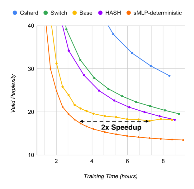
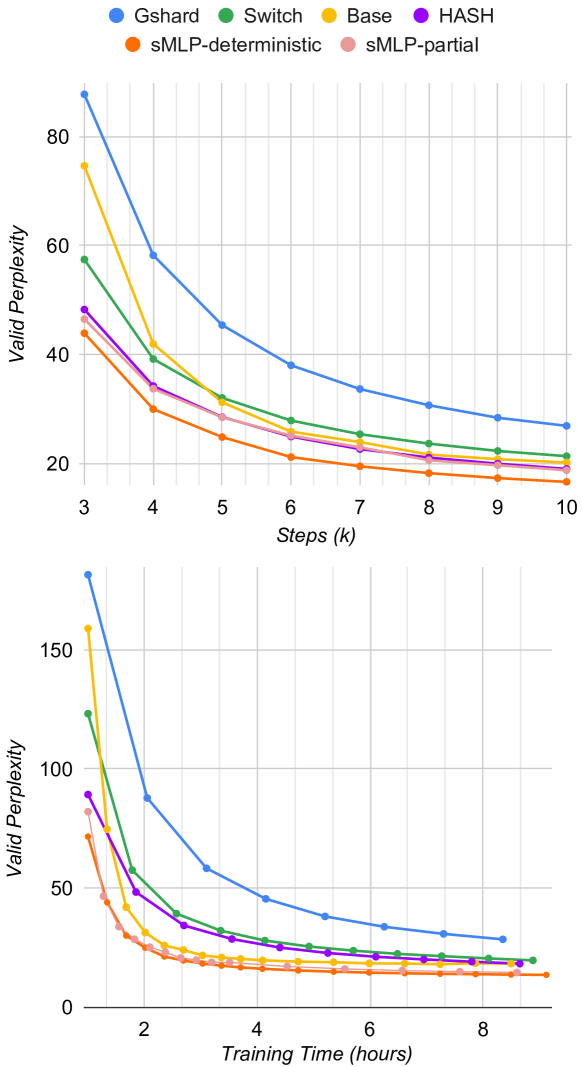
• We empirically evaluate its performance on language modeling and compare with strong baselines of both sparse Transformer-based MoEs such as Gshard (Lepikhin et al., 2020), Switch Transformer (Fedus et al., 2021), Base Layers (Lewis et al., 2021) and HASH Layers (Roller et al., 2021) as well as dense models including Transformer (Vaswani et al., 2017b) and gMLP (Liu et al., 2021a). Our sMLP outperforms these models in terms of valid perplexities while obtaining up to 2 $\times$ improvement in pretraining speed with the same compute budget (shown in Fig. 1). In addition, sMLP demonstrates good scalability where it still outperforms sparse Transformers counterparts when we scale sMLP to 10B parameters with a large pretraining corpus of 100B tokens.

• Finally, we evaluate its zero-shot priming performance after pretraining on language modeling. Through head-to-head comparison, the proposed sparsely-activated all-MLP language model outperforms sparsely-activated Transformers on six downstream tasks ranging from natural language commonsense reasoning to QA tasks. Compared with dense Transformers such as GPT-3 (Brown et al., 2020b), our sMLP model achieves similar zero-shot performance despite being pretrained on a much smaller dataset (3 $\times$ smaller than the dataset used by GPT-3) with less computing resources.

Figure 1: The proposed sparse all-MLP architecture (sMLP) achieves 2$\times$ training efficiency improvement compared to state-of-the-art sparse Transformer-based MoEs: Gshard(Lepikhin et al., 2020), Switch Transformer (Fedus et al., 2021), Base Layers (Lewis et al., 2021), HASH Layers (Roller et al., 2021). Full comparison is provided in Fig. 5.

Figure 2: Illustration of sMLP Model Architecture with $N_{1}$ Dense Blocks (gMLP layers) and $N_{2}$ Sparse Blocks. The arrangement of these blocks will be discussed in Section 4.1. Each sparse block contains a tMoE module and a sMoE module. The tMoE module sparsely activated FFN (feed-forward) and the sMoE module replaces the self attention in Transformers with sparse token-wise SL (spatial linear projection) operations.

2 Background

2.1 Token-wise Operations

Transformers and all-MLPs perform token-mixing operations in different ways. The former uses self-attention (Vaswani et al., 2017b), while the latter uses Spatial Gating Unit (Liu et al., 2021a).

Given the input token representation $X\in\mathbb{R}^{T\times H}$, where $T$ represents the sequence length and $H$ represents the hidden dimension. We set $h$ to be the total head number.

Self attention module

The multi-head self attention module is a concatenation of token-mixing operations from each head:

$$Y =\operatorname{Concat}\left(M_{1},\ldots,M_{\mathrm{h}}\right)$$ (1)

$$\text{ with }M_{\mathrm{i}} =\operatorname{Softmax}(XW_{i}^{Q}\ XW_{i}^{K})XW_{i}^{V}$$

where $Y$ is the output, $W_{i}^{Q},W_{i}^{K},W_{i}^{V}\in\mathbb{R}^{H\times d}$ are projection matrices. $d$ is the hidden dimension for input to a single head $d=H/h$.

Spatial Gating Unit

gMLP (Liu et al., 2021a) designs the Spatial Gating Unit to replace the self attention module. Within each head,

$$Y=W_{s}X$$ (2)

, where $W_{s}\in\mathbb{R}^{T\times T}$. Note that, $W_{s}$ corresponds to the attention score instead of $W^{V}$ in Equation (1).

2.2 Sparse Expert Models

Sparse expert models provide a highly efficient way to scale neural network training. Compared to the standard dense models that require extremely high computational cost in training, sparse expert models are shown to be able to deal with a much larger scale of data and converge significantly faster. In sparse models, model weights are distributed to different workers according to the MoE mechanism (Lepikhin et al., 2020; Fedus et al., 2021; Lewis et al., 2021; Roller et al., 2021; Yang et al., 2021). The standard MoE was initially being designed for the feed-forward module, which leverages a routing algorithm to dispatch each token to $k$ sub feed-forward modules. These sub feed-forward modules are allocated independently on different devices, which are also called experts. MoE allows processing input tokens in parallel specified by a gating function to achieve maximum computational efficiency.

MoE Routing

Let $\{E_{i}(x)\}_{i=1}^{N}$ be a set of $N$ experts for a token representation $x$. Shazeer et al. (2017) proposed a MoE layer that learns to dispatch the token representation to the best determined top-$k$ experts, selected from a set $\{E_{i}(x)\}_{i=1}^{N}$ of $N$ experts. The router variable $W_{r}$ produces logits $h(x)=x\cdot W_{r}$ which are normalized via a softmax distribution over the available $N$ experts at that layer. The gate-value for expert $i$ is given by,

$$p_{i}(x)=\frac{e^{h(x)_{i}}}{\sum_{j=1}^{N}e^{h(x)_{j}}}$$ (3)

The top-$k$ gate values are selected for routing the token $x$. If $\mathcal{T}$ is the set of selected top-$k$ indices then the output computation of the layer is the linearly weighted combination of each expert’s computation on the token by the gate value,

$$y=\sum_{i\in\mathcal{T}}p_{i}(x)E_{i}(x)$$ (4)

Given that each token will be sent to different devices (experts), unbalanced loading adds heavy affects the efficiency of the model. The Switch Transformer (Fedus et al., 2021) designed a differential load balancing loss to reduce communication latency of sending tokens to different devices. Base Layers (Lewis et al., 2021) further simplify the framework by eliminating the balancing loss, adapting the balancing assignment algorithm (Bertsekas, 1992) to send tokens from each batch to different devices equally. Instead of learning the routing weight $W_{r}$, HASH Layers (Roller et al., 2021) use a random hashing function as the routing gate. In order to distinguish this standard Transformer-MoE routing (Lepikhin et al., 2020; Fedus et al., 2021; Lewis et al., 2021; Roller et al., 2021; Yang et al., 2021) from ours, we call this method tMoE.

3 Methods

A straightforward extension of gMLP to MoE structure hurts performance, which we provide a detailed analysis in Appendix A. Instead of sending tokens to different experts, in Section 3.1 we propose a novel sMoE module to send hidden vectors to different experts. We further propose two corresponding routing strategies in Section 3.2.1 and Section 3.2.2.

3.1 Sparsely-activated all-MLP

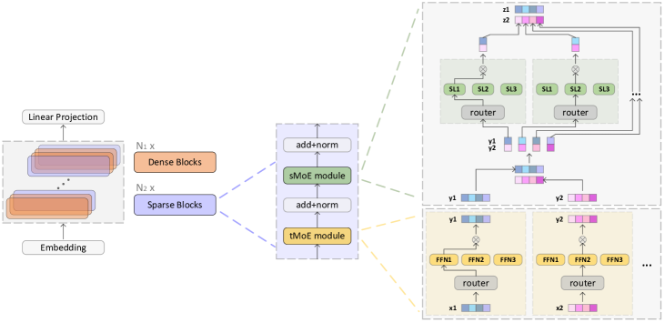
The overall architecture of sMLP is illustrated in Fig. 2. Our sMLP model contains $N_{1}$ dense blocks and $N_{2}$ sparse blocks. Both $N_{1}$ and $N_{2}$ are hyper-parameters. In each sparse block, it contains two modules: $(\textup{\it i})$ tMoE module: we adopt the MoE from Base Layers (Lewis et al., 2021) to replace the FFN module in dense Transformers (Vaswani et al., 2017b); $(\textup{\it ii})$ sMoE module: we design this sMoE module to replace the self attention module in the Transformer (Vaswani et al., 2017b) and the Spatial Gating Unit in gMLP (Liu et al., 2021a);

Both tMoE and sMoE blocks contain two elements:

Expert Modules

These are the modules that process the input. The tMoE module contains an FFN in each expert. For our sMoE module, each expert contains the Spatial Gating Unit as is shown in Fig. 6 (Right) in Appendix A.

Gating Function

This is the module that decides which expert should process each part of the input. tMoE uses standard token-wise routing (described in Section 2.2). However, naively applying token-wise routing to gMLP is flawed, as it sends tokens from the same sentence to different experts. Tokens can only attend to previous tokens in the same device, which means that as the number of experts increases, the number of previous tokens that each word can attend will decrease. Refer to Appendix A for more details. For that reason, we have to design a distinct routing method to extend the MoE structure to the feature dimension.

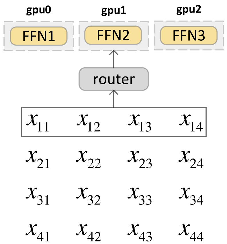
Fig. 3 (Left) shows an example of the gating function from existing Transformer-based MoEs (Lepikhin et al., 2020; Fedus et al., 2021; Lewis et al., 2021; Roller et al., 2021). $x_{ij}$ denotes the value of the $j_{th}$ hidden dimension in the $i_{th}$ tokens. The tMoE sends these four tokens to these three experts at the FFN layer using a learnt gating function described in Eq.(3) parameterized by $W_{r}\in\mathbb{R}^{4\times 3}$.

Unlike these existing MoEs, in sparse all-MLP architecture we propose to chunk hidden representation along the hidden dimension and send chunked vectors to different experts, as is shown in Fig. 3 (Right). We next discuss the design of the gating function for this new routing mechanism.

3.2 Routing in Feature Space

Compared to routing tokens, routing hidden dimensions faces a unique challenge in autoregressive models, with information leaking from looking ahead at future tokens if done naively (more details can be found in Appendix B.). Furthermore, unlike Transformers-based MoEs with self-attention, appropriate masking cannot be directly applied to prevent information leaking. Due to the aforementioned problems, we cannot adopt existing routing methods in Transformers-based MoEs for language modeling. We propose and compare the following two solutions: deterministic routing and partial prediction.

Figure 3: Left: tMoE Gating: sending 4 tokens to 3 experts; Right: sMoE Gating: sending 4 hidden vectors to 3 experts.

3.2.1 Deterministic Routing

In order to decide where to send different hidden vectors, we need to learn a gating weight $W_{r}\in\mathbb{R}^{T\times N}$. This gating weight inevitably needs to multiply the hidden vector $v$ to obtain the routing probability $p_{i}(v)$. This vector is one specific hidden dimension of the whole sentence, including future tokens.

In order to prevent the gating weights from exploiting future token information, which is not available at inference time, our first approach removes $W_{r}$ directly. Instead, we chunk the vector in a hidden dimension and send hidden vectors to experts deterministically. In this case, if we want to send the hidden vector $V\in\mathbb{R}^{H\times T}$ to $N$ expert modules, we will chuck $h(v)_{i}\in\mathbb{R}^{H/N\ \times\ T}$ from hidden vector $V$. If $i$ equals to $0$, the gating will send the first to $H/N$ hidden vectors to $E_{1}(v)$.

Unlike the Spatial Gating Unit, our attention-free sMoE-deterministic module splits the hidden dimensions among multiple experts. In each expert module, we insert one Spatial Gating Unit, similar to multi-head attention, where each expert serves as one head. The total number of parameters is $N*T*T$ where $N$ is the number of experts/heads. Moreover, with each head being fitted to one device, the computation is parallel.

3.2.2 Partial Prediction

Another way to prevent the gating weight $W_{r}$ from using future token information is partial prediction. Instead of predicting all the tokens in the sentence, we condition on the first $20\%$ of tokens, which are used to decide the routing, and predict the remaining $80\%$ of tokens.

Given the input token representation $X\in\mathbb{R}^{T\times H}$, we divide it into two parts in the token dimension: the first $20\%$ of tokens $X_{1}\in\mathbb{R}^{0.2T\times H}$, and the remaining $80\%$ of tokens $X_{2}\in\mathbb{R}^{0.8T\times H}$. Instead of training the language model on the whole sequence length $T$, we only train it to predict $X_{2}$. We use $X_{1}$ to learn the gating weights $W_{r}$. In sMoE, we transpose theinput $X_{1}$ to $V_{1}\in\mathbb{R}^{H\times 0.2T}$, input $X_{2}$ to $V_{2}\in\mathbb{R}^{H\ \times\ 0.2T}$. The router variable $W_{r}\in\mathbb{R}^{0.2T\times N}$ produces $h(V_{1})=V_{1}*W_{r}$. $V_{1}$ contains $H$ hidden vectors $v_{i}\in\mathbb{R}^{0.2T}$. The probability for sending $i_{th}$ hidden vector is learned by

$$p_{i}(v)=\frac{e^{h(v)_{i}}}{\sum_{j}^{N}e^{h(v)_{j}}}$$ (5)

Different from the previous method, after learning the probability $p_{i}(v)$, this partial prediction method sends hidden vectors $v_{i}\in\mathbb{R}^{0.8T}$ from $V_{2}$ to the expert module instead of hidden vectors from $V_{1}$.

4 Experiments and Results

4.1 Experimental Setup

Baselines

We compare to strong baselines consisting of state-of-the-art dense and sparse models, as is summarized in Table 1. We train all our baselines (except GPT3 from paper) and our model in PyTorch (Paszke et al., 2017) using FAIRSEQ (Ott et al., 2019).

Baselines	Model
Dense Baselines	Transformer (Vaswani et al., 2017b) gMLP (Liu et al., 2021a)
Sparse Baselines	Gshard (Lepikhin et al., 2020) Switch Transformer (Fedus et al., 2021) Base Layers (Lewis et al., 2021) HASH Layers (Roller et al., 2021)

Table 1: Baselines: we compare our sMLP with dense Transformers and MLPs as well as sparse Transformer-based MoEs.

Experiments	FLOPs	Model Size	Datasets
Main Experiments	0.8T	3.50B	1/10 data from RoBERTa dataset (Liu et al., 2019)
Scalability Experiments	2.0T	9.41B	$\sim$ 100B tokens. RoBERTa and the English subset of the CC100 corpus (Conneau et al., 2019)

Table 2: Experimental Settings: In Section 4.3, we run our small model (3.50B parameters) with FLOPs per batch tokens 0.8T on the small dataset (1/10 of the RoBERTa dataset); In Section 4.4, we run our large model (9.41B parameters) with FLOPs per batch tokens 2.0T on the whole RoBERTa dataset plus CC100 corpus.

Modules	heads	params.(M)	FLOPs (G)
Self-attention	16	4.198	12.885
Self-attention	1	4.198	12.885
Spatial Gating Unit	16	16.798	4.316
Spatial Gating Unit	1	1.054	4.316
s-MoE	1	1.058	4.387

Table 3: Token-wise Operations Comparison: we compare our method with the previous two token-wise operations regarding parameters and FLOPs by each operation.

Models	Model Size (Parameters)	Quality after 25k steps (Perplexity $\downarrow$)	Time to Quality (hours $\downarrow$)	Speed (world per second $\uparrow$)
Gshard (Lepikhin et al., 2020)	3.48B	19.26	27.54	136k
Switch Transformer (Fedus et al., 2021)	3.48B	15.31	20.67	185k
Base Layers (Lewis et al., 2021)	3.60B	18.16	21.13	178k
HASH Layers (Roller et al., 2021)	3.51B	13.57	21.08	176k
sMLP – deterministic (our model)	3.50B	13.46	20.41	192k

Models	Model Size (Parameters)	Quality after 100k steps (Perplexity $\downarrow$)	Time to Quality (hours $\downarrow$)	Speed (world per second $\uparrow$ )
Gshard (Lepikhin et al., 2020)	9.03B	14.5	198	115k
Switch Transformer (Fedus et al., 2021)	9.03B	10.45	120	139k
Base Layers (Lewis et al., 2021)	10.31B	20.36 (divergence)	115.13	135k
HASH Layers (Roller et al., 2021)	10.29B	16.69	100	141k
Switch Transformer - Enlarge (FLOPs 2.3T)	10.31B	10.09	140	126k
sMLP – deterministic (our model)	9.41B	9.84	112	144k

Table 4: Head-to-head comparison measures per step and per time benefits of the sMLP (our model) over baselines. We report perplexity (lower better) and time to reach (lower better) as quality and training efficiency measures. All models are trained with the same amount of computation and hardware. In order to test parameter-matched models, we train an enlarged Switch Transformer with 2.0T FLOPs. Top: Small models (FLOPs 0.8T). Bottom: Scaled-up models (FLOPs 2.0T). More model details are described in Table 5.

Figure 4: Comparison with Dense Models: We compare our model (the orange dashed line) with dense models (solid lines), including both Transformer (Vaswani et al., 2017a) and gMLP (Liu et al., 2021a), with different heads. Our model (sMLP) only has one head activated on each device.

Experimental Settings and Dataset

A sparsely activated model splits unique weights on different devices. Therefore, the weights of the model increase with the number of devices, all while maintaining a manageable memory and computational footprint on each device. Previous work (Lepikhin et al., 2020; Fedus et al., 2021; Yang et al., 2021) controls the floating point operations (FLOPs) per example for model comparison. We utilize the fvcore library to measure the floating point operations (FLOPs) per batch tokens during evaluation for model comparison. Since all models contain exactly the same tokens in each batch, we actually controls FLOPs per token.

Our experimental settings are summarized in Table 2. $(\textup{\it i})$ we compare to all baselines in a regular setting. In order to control for FLOPs, we change the number of layers in the model. More concretely, since Gshard (Lepikhin et al., 2020) and Switch Transformer (Fedus et al., 2021) have larger FLOPs values for the same model structure, we reduce their number of layers while keeping the same hidden dimension to achieve the same FLOPs. $(\textup{\it ii})$ we also conduct experiments at larger scale and data size to test its scalability. We use pretraining datasets from RoBERTa (Liu et al., 2019) and the English portion of CC100 (Conneau et al., 2019). More details can be found in Appendix C.3.

Figure 5: Top: Valid Perplexity v.s. Training Steps; Bottom: Valid Perplexity v.s. Training Time. We compare our two methods (sMLP-deterministic and sMLP-partial) with sparse Transformer MoEs with 0.8T FLOPs.

Metrics

(1). Language modeling perplexity: We report validation perplexity as the indicator of language modeling performance. (2). Training efficiency: For measuring training speed and efficiency, we compare by both number of updates and word-per-second (WPS). (3). Accuracy: we report accuracy on downstream tasks to measure performance of zero-shot priming.

Models	FLOPs (T)	Model Size (M)	Embedding Dim	Hidden Dim	Sparse Layers	Dense Layers	Num of Heads	Num of Experts	Num of GPUs
Gshard	2.0	9.03	2048	8192	7	7	16	64	32
Switch Transformer	2.0	9.03	2048	8192	7	7	16	32	32
Base Layers	2.0	10.31	2048	8192	8	8	16	32	32
HASH Layers	2.0	10.29	2048	8192	8	8	16	32	32
Switch Transformer - Enlarge	2.3	10.31	2048	8192	8	8	16	32	32
sMLP – deterministic (our model)	2.0	9.41	2048	8192	7	22	1	32	32

Table 5: Scaled-up Model details: We control FLOPs to the same level by adjusting the number of layers of the model. Since our model is based on gMLP (Liu et al., 2021a), more dense layers are needed, and only one head is needed for each device. While controlling FLOPs value, we found that only the Switch Transformer (Fedus et al., 2021) can be compared with our sMLP among all the baselines. With the same amount of FLOPs value, our model has more parameters than the Switch Transformer; then, we train a Switch Transformer - Enlarge model for comparison.

Implementation

Our sMLP model contains $N_{1}$ dense blocks and $N_{2}$ sparse blocks. We follow Base Layers (Lewis et al., 2021) setting: insert sparse blocks after the $\lfloor\frac{(N_{1}+N_{2})}{N_{2}+1}\rfloor\dots\lfloor\frac{N_{2}(N_{1}+N_{2})}{N_{2}+1}\rfloor$th dense layers. For sparse blocks, it contains one tMoE module and one sMoE module. We adopt tMoE modules from Base Layers (Lewis et al., 2021). For our sMoE module, in each expert module, we insert one Spatial Gating Unit. Among our baselines, Base Layers (Lewis et al., 2021) and HASH Layers (Roller et al., 2021) adopt the same approach to arranging sparse layers. In contrast, Gshard (Lepikhin et al., 2020) and Switch Transformer (Fedus et al., 2021) insert a sparse module at every other layer. More details of model architectures and implementation details can be found in Appendix C.

4.2 Token-wise operations comparison

In this section, we compare our model with two dense models: Transformer (Vaswani et al., 2017b) and gMLP (Liu et al., 2021a). The main difference between the all-MLP-based and the Transformer-based models is the token-wise operation. We compare these three kinds of token-wise operations: the self-attention module in Transformers, the Spatial Gating Unit in gMLP, and the sMoE module in our model.

In Table 3, we compare these three token-wise operations and their respective head mechanisms. To extend multi-head mechanism into gMLP mode, instead of using one $W_{s}$ in Equation (2), we chunk the input $X$ into $h$ parts along hidden dimension, and each part is multiplied by a separate $W_{s}$. We set head number $h$ to be 16 to compare Spatial Gating Unit from gMLP with Self-attention module from Transformer. Then the total number of parameters is $h*T*T$. Compared to Transformer self attention, a shortcoming of the Spatial Gating Unit is that the number of parameters increases linearly with the number of heads $h$ and quadratically with sequence length $T$. For comparison, our s-MoE module set one expert on each device, and each expert only contains one $W_{s}$, which is equal to heads number 1.

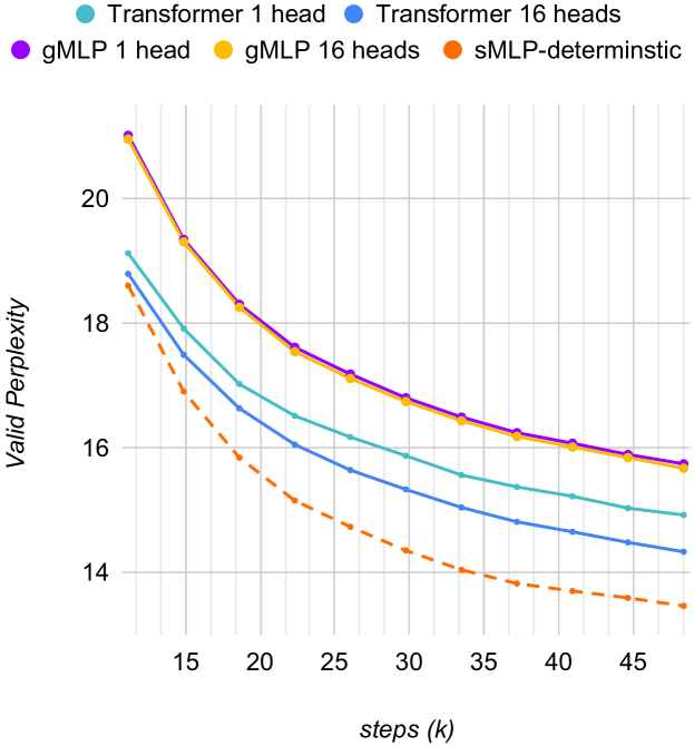
In Fig. 4, we compare our model with the dense model with different heads number. The Transformer model greatly benefits from the multi-head mechanism. However, although the gMLP model increases the parameter amount, it does not improve performance through the multi-head mechanism. Our model can also be seen as a solution for gMLP’s multi-head. Our model dramatically improves the performance of the all-MLP-based model and also outperforms the Transformer model.

4.3 Results on Sparse MLP

We report quality (valid perplexity) and training efficiency in Fig. 5, measured by number of training steps (Top) and training time (Bottom). We found that sMLP with both variants of routing strategies outperforms state-of-the-art Transformer-based MoE models with roughly the same amount of FLOPs. We point out that sample efficiency observed on a step basis does not necessarily translate into better model quality as measured by the wall clock due to two reasons. First, our model has additional all2all communication cost for sMoE module. Second, Base Layers, HASH Layers, and our model send tokens/vectors to the expert module in a balanced manner. In contrast, Gshard and Switch Transformer leverage a loss function to balance the assignment, which is not an equally balanced assignment. Although they have the same FLOPs, unbalanced loading can add extra computing time. Fig. 5 (Bottom) shows that given the same training time, our model achieves the best results (lowest valid perplexity), indicating that our sparse all-MLP models improved training efficiency over state-of-the-art Transformer-based MoE models on language modeling.

Table 4 (Top) summarizes the detailed comparison in the main experiments. We control the FLOPs of all models to be roughly 0.8T. Except that the number of model layers is different, their embedding dimension is 1024, and the hidden dimension is 4096. We can see that our model achieves the best generalization at 25k training steps and in the meanwhile achieves the highest training speed. HASH Layers has the best performance among all Transformer baselines and requires the least time, which is consistent with results reported in Roller et al. (2021).

4.4 Evaluation on Scalability

In order to test the scalability of our model, we increase the model size training for 2.0 TFLOPs. Table 4 (Bottom) summarizes the results.

Compared to models in Table 4 (Top), we enlarged all of the models, changing the embedding from 1024 to 2048, and adjusting the hidden dimension from 4096 to 8192 as reported in Table 5. We also increased the pretraining data size as described in Table 2.

In this setting, we found Switch Transformer to remain a strong baseline. Although Base Layers and HASH Layers perform well when trained on small models and datasets, we find stability issues on large-scale training. Although previous papers (Fedus et al., 2021; Lepikhin et al., 2020) have controlled the FLOPs for model comparison, we found the FLOPs-match Switch Transformer has fewer parameters than our model. Therefore, to provide a more fair comparison, we also trained an enlarged version of Switch Transformer (by adding one additional sparse layer and dense layer) with 10.31B parameters which also increases its FLOPs to 2.3T. Our sMLP still outperforms Switch Transformer-Enlarge despite the latter having more FLOPs.

Models	COPA	PIQA	StoryCloze	Winogrande	HellaSwag	ReCoRD	Average
GPT-3 (Brown et al., 2020b) from paper	73.0	72.9	72.4	57.4	51.0	82.1	68.13
Gshard (Lepikhin et al., 2020)	76.00	68.12	67.88	51.068	38.00	72.39	62.24
Switch Transformer (Fedus et al., 2021)	75.0	72.96	73.33	53.43	52.48	79.86	67.84
Base Layers (Lewis et al., 2021)	63.00	63.82	61.41	50.98	30.22	60.70	55.02
HASH Layers (Roller et al., 2021)	64.00	63.77	64.72	51.70	33.04	67.15	57.40
sMLP – deterministic (our)	79.00	72.96	74.67	54.31	54.53	73.42	68.15

Table 6: Zero-shot priming evaluation: we provide head-to-head comparison of our sMLP model with FLOPs-matched state-of-the-art sparse Transformers on six representative NLP tasks evaluated in GPT-3 in-context learning(Brown et al., 2020b). Specifically, we control for training data, batch size, learning rate and training steps for all these models. As a reference point, we also compare to the performance of a FLOPs-matched GPT3 model (dense Transformer) reported in Brown et al. (2020b). Note that the GPT3 model from the paper uses larger training dataset (about 3 $\times$ larger).

4.5 Zero-shot Priming

The previous experiments demonstrate sMLP’s strong performance in language modeling. In this section, we evaluate whether these gains in pretraining translate to improved generalization in downstream tasks. Specifically, we measure zero-shot in-context learning capability as is shown in GPT-3 (Brown et al., 2020b).

Baselines

Our baselines are Gshard (Lepikhin et al., 2020), Switch Transformer (Fedus et al., 2021), Base Layers (Lewis et al., 2021) and HASH Layers (Roller et al., 2021) with roughly 2.0 TFLOPs from Section 4.4.

Tasks and datasets

We select six representative NLP tasks which probes commonsense reasoning and question answering, including COPA (Roemmele et al., 2011), PIQA (Bisk et al., 2020), StoryCloze (Mostafazadeh et al., 2016), Winogrande (Levesque et al., 2012), HellaSwag (Zellers et al., 2019), ReCoRD (Zhang et al., 2018). We use a language model to separately score each label choice using the same templates, and pick the one with the highest score as Artetxe et al. (2021). More details about tasks and datasets can be found in Appendix E.

Results

As is shown in Table 6, sMLP outperforms all sparse Transformers in terms of average accuracy. Notable improvements come from commonsense reasoning tasks such as COPA, StoryCloze and HellaSwag. We also compared to a FLOPs-matched dense Transformer reported in the GPT-3 paper (Brown et al., 2020b), which served as the strongest dense baseline. It is worth noting that the GPT-3 model was trained with more pre-training data (GPT-3 used 300 billion tokens for pre-training and our pre-training data contains 100 billion tokens).

5 Related Work

Mixture of Experts (MoE) was shown to be effective in Shazeer et al. (2017), where an MoE layer was stacked between LSTM (Hochreiter & Schmidhuber, 1997) layers. More recently, Gshard (Lepikhin et al., 2020) extended this idea to Transformer (Vaswani et al., 2017b) feed-forward layers and provided a way for parallel computing, which scaled up multilingual neural machine translation with Sparsely-Gated Mixture-of-Experts beyond 600 billion parameters using automatic parameter sharding.

Several recent work improves the routing strategy in Transformer-based MoEs. Switch Transformer (Fedus et al., 2021) shows the design can be simplified by routing tokens to only one single expert (top-1 routing). In addition, they design a differentiable load balancing loss to reduce communication latency of sending tokens to different devices. Base Layers (Lewis et al., 2021) further simplifies the framework by eliminating the balancing function, adapting the balancing assignment algorithm (Bertsekas, 1992) to send tokens from each batch to different devices equally. Instead of learning the gating weights for token assignment, HASH Layers (Roller et al., 2021) design a Hash function to replace the learnable gating weights. (Jaszczur et al., 2021) is the first one successfully extending sparsity to attention layers. However, their results could just match dense transformer and did not get improvements in training speed. Different from all of the above routing methods, our sMoE-deterministic method (described in Section 3.2.1) chunk vectors by deterministic assignment.

There is also a growing body of work studying the overall design and scaling of Transformer-based MoE models. Yang et al. (2021) explores key factors inside sparse expert models and investigates how they affect the model quality and computational efficiency. Clark et al. (2022) studied the scaling laws of MoE models in terms of effective parameter count and compared three routing strategies. Zoph et al. (2022) investigated several training details which affects training stability and finetuning performance. In addition to NLP, Riquelme et al. (2021) firstly applied MoEs in the Computer Vision field.

A closely related work is Lou et al. (2021), which developed all-MLP-based MoEs for computer vision. When applied to NLP, there are additional challenges in designing the sparsely activated token-mixing operations by preserving the sequential nature of the input, which would otherwise lead to information leaking as is shown in Section 3.2.

6 Conclusion

In this work, we proposed sMLP, extending the recent gMLP (Liu et al., 2021a) model with sparsely activated conditional computation using mixture-of-experts (MoEs). Different from Transformer-based MoEs, which only contains sparse feed-forward layers while still keeping dense computation for self-attention, the proposed architecture is fully sparse. We analyzed the challenges in designing routing strategies of sparse all-MLP architecture for language modeling and proposed two solutions. Through extensive evaluations on language modeling, we show that sMLP outperforms state-of-the-art sparse Transformer-based MoE models in terms of generalization and 2$\times$ improvement in training efficiency. Besides gains in pretraining, sMLP also achieves higher accuracy in zero-shot in-context learning of six representative NLP tasks, closing the gap of all-MLP architecture with Transformers as was observed in gMLP. It is worth noting that all our discussions about routing challenges and solutions are based on autoregressive language modeling. In the future, we hope to try all-MLP based MoE method with encoder-only models with bidirectional attention.

Appendix A Direct applying token-wise routing to gMLP

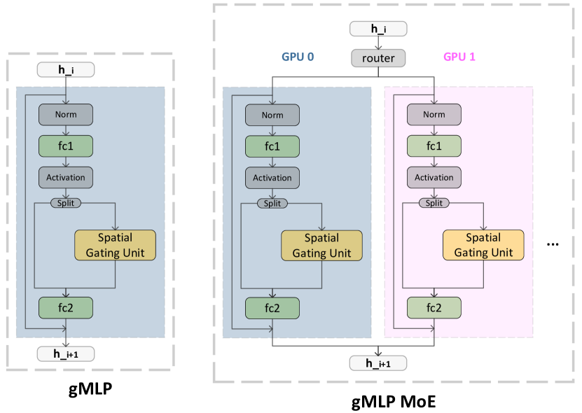
The most straightforward way to extend gMLP (Liu et al., 2021a) to mixture-of-experts (MoEs) is to apply the same token-routing used in Transformer-based MoEs (Lepikhin et al., 2020; Fedus et al., 2021; Lewis et al., 2021; Roller et al., 2021), as is illustrated in Fig. 6 in the case of two experts (GPUs).

Figure 6: Left: one layer of gMLP(Liu et al., 2021a); Right: directly extend gMLP to token-level conditional computation commonly used in Transformer MoEs (Lepikhin et al., 2020; Fedus et al., 2021; Lewis et al., 2021; Roller et al., 2021) with two experts (GPUs).

Models	# Experts	Valid Perplexity
gMLP	0	15.7
gMLP MoE	32	17.2
gMLP MoE	64	20.5

Table 7: Extending gMLP to token-based MoEs hurts performance compared to dense gMLP. Furthermore, increasing the number of experts worsens the performance.

Table 7 shows that this approach, despite being simple and straightforward, has poor generalization. Since the Spatial Gating Unit is inserted into each device, and the tokens from the same sentence will be sent to different devices. That means tokens can only attend to previous tokens which were sent to the same device. This problem will be more severe as we increase expert (device) numbers. As the number of experts increases, the probability of sending tokens to the same expert from one sentence will decrease, so the number of tokens that each word can attend will decrease.

Figure 7: Compared sMLP method with sMLP – deterministic (Section 3.2.1) and sMLP – partial (Section 3.2.2)

Appendix B Gating analysis for the sMLP module

MoE layers take token representation $X\in\mathbb{R}^{T\times H}$, where $T$ represents the sequence length and $H$ represents the hidden dimension. In the sMoE, we transpose input to the hidden vector $V\in\mathbb{R}^{H*T}$. A gating function routes this to the best top-$k$ experts, selected from a set $\{E_{i}(v)\}_{i=1}^{N}$ of $N$ experts. The router variable $W_{r}\in\mathbb{R}^{T\times N}$ produces $h(V)=VW_{r}$ which are normalized via a softmax distribution over the available $N$ experts at that layer. $V$ contains $H$ hidden vector $v_{i}\in\mathbb{R}^{T}$. The probability for sending $i_{th}$ hidden vector is given by

$$p_{i}(v)=\frac{e^{h(v)_{i}}}{\sum_{j}^{N}e^{h(v)_{j}}}$$ (6)

The top-$k$ gate values are selected for routing the hidden vector $v$. If $\mathcal{T}$ is the set of selected top-$k$ indices then the output computation of the layer is the linearly weighted combination of each expert’s computation on the token by the gate value,

$$y=\sum_{i\in\mathcal{N}}p_{i}(v)E_{i}(v)$$ (7)

Through learning the gating weight $W_{r}$, the MoE model routes hidden vectors to different experts.

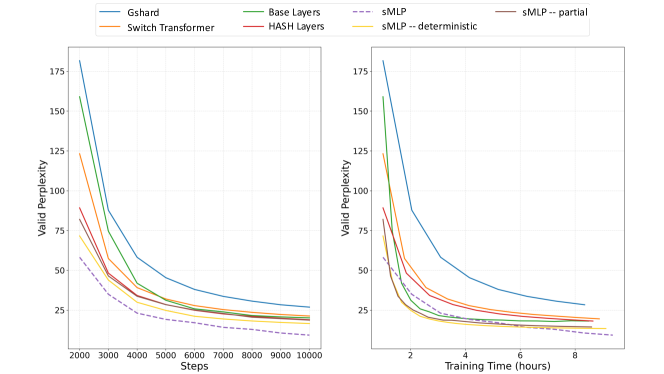
Fig. 7 shows the results by this method (sMLP in the figure). We can see that this method achieves the lowest perplexity. However, this is due to information leaking from future tokens in learning $W_{r}$. Specifically, the gating weight for sMoE is $W_{r}\in\mathbb{R}^{T\times N}$, which is trained after seeing all the tokens in the sentence, especially looking ahead at future tokens. In this way, this gating can making ”smartest” decision. This results in information leaking for autoregressive language models. Unlike self attention model, where a diagonal mask could be applied to attention scores $A\in\mathbb{R}^{T\times T}$ to prevent information leaking from future tokens, gating weights $W_{r}\in\mathbb{R}^{T\times N}$ cannot use a valid mask. Due to the aforementioned problems, we cannot adopt existing MoE gating methods for routing hidden vectors in autoregressive language models. Therefore, we propose two improved methods sMLP – deterministic (in Section 3.2.1) and sMLP –partial (in Section 3.2.2).

Appendix C More implementation details

C.1 Choice of baselines

The dense counterpart is gMLP (Liu et al., 2021a). We adapted the balanced assignment routing method proposed in Base Layers (Lewis et al., 2021) for the tMoE implementation. Thus, the closest Transformer-based sparse models is Base Layers (Lewis et al., 2021). We also compared to the dense Transformer (Vaswani et al., 2017b) and other state-of-the-art Transformer MoE models (Gshard (Lepikhin et al., 2020), Base Layers (Lewis et al., 2021), HASH Layers (Roller et al., 2021)) as listed in Table 1.

C.2 Training

Small Model Configurations

Table 8 shows the the detailed model architecture used in the main experiments. Through observation, we noticed that all the models (except for Gshard) drop negligibly after 15k. In addition, there is a small amount of fluctuation for the Base Layers after 25k. Then we choose 25k for model comparison in Table 4.

Models	Base Layers	sMLP-deterministic
Expert Parameters	100.75 M	113.44 M
Non Expert Parameters	241.79 M	258.73 M
FLOPs	0.83 T	0.83 T
Expert Modules per MoE layer	32	32
Number of MoE layers	12	12
FFNs per Expert Module	1	1
Spatial Gating Unit per Expert Module	1	1
Embedding Size	1024	1024
Hidden Dimension	4096	4096
Heads	16	1
Number of Dense Layers	12	28
Context Length	1024	1024
Batch Size	4	4
Gradient Accumulation	4	4
Dropout	0.1	0.1
ddp-backend	no_c10d	no_c10d
optimizer	adam	adam
adam-betas	(0.9, 0.98)	(0.9, 0.98)
weight-decay	0.1	0.1
lr	5e-4	5e-4
lr-scheduler	inverse_sqrt	inverse_sqrt
warmup-updates	4000	4000
warmup-init-lr	1e-7	1e-7

Table 8: Model architectures used in the main experiments in Section 4.3.

Models	Transformer	gMLP	sMLP-deterministic
Expert Parameters	0 M	0 M	258.73M
Non Expert Parameters	354.76 M	353.87 M	113.44M
FLOPs	0.83 T	0.83 T	0.83 T
Sparse Layers	0	0	12
Dense Layers	24	41	28
Embedding Size	1024	1024	1024
Hidden Dimension	4096	4096	4096
Heads	16	1	1
Context Length	1024	1024	1024
Batch Size	2	2	2
Gradient Accumulation	4	4	4
Dropout	0.1	0.1	0.1
ddp-backend	no_c10d	no_c10d	no_c10d
optimizer	adam	adam
adam-betas	(0.9, 0.98)	(0.9, 0.98)	(0.9, 0.98)
weight-decay	0.1	0.1	0.1
lr	5e-4	5e-4	5e-4
lr-scheduler	inverse_sqrt	inverse_sqrt	inverse_sqrt
warmup-updates	4000	4000	4000
warmup-init-lr	1e-7	1e-7	1e-7

Table 9: Small dense model architectures used in Section 4.2.

Large model configuration

Table 10 shows the the model architecture used in scalability experiments. Through observation, we noticed that all the models (except for Base Layers) are converged around 70k. After 70k, these models drop negligibly. Then we choose 100k for model comparison in Table 4.

Models	Base Layers	sMLP-deterministic
Expert Parameters	642.6 M	682.6 M
Non Expert Parameters	268.6 M	277.1 M
FLOPs	2.125 T	2.125 T
Expert Modules per MoE layer	32	32
Number of MoE layers	8	8
FFNs per Expert Module	1	1
Spatial Gating Unit per Expert Module	1	1
Embedding Size	2048	2048
Hidden Dimension	8192	8192
Heads	16	1
Number of Dense Layers	8	20
Context Length	1024	1024
Batch Size	2	2
Gradient Accumulation	8	8
Dropout	0.1	0.1
ddp-backend	no_c10d	no_c10d
optimizer	adam	adam
adam-betas	(0.9, 0.98)	(0.9, 0.98)
weight-decay	0.1	0.1
lr	1e-3	1e-3
lr-scheduler	inverse_sqrt	inverse_sqrt
warmup-updates	4000	4000
warmup-init-lr	1e-7	1e-7

Table 10: Large model architectures used in the scalability experiments in Section 4.4 and Section 4.5.

Dense model configuration

Table 9 shows the model architecture we use in Section 4.2.

All the models are trained on 32 Nvidia 32G V100 GPUs.

C.3 Datasets

The RoBERTa contains five English-language corpora of varying sizes and domains:

• BOOKCORPUS (Zhu et al., 2015) plus English WIKIPEDIA. This is the original data used to train BERT. (16GB).

• CC-NEWS, which collected from the English portion of the CommonCrawl News dataset (Nagel, 2016). The data contains 63 million English news articles crawled between September 2016 and February 2019. (76GB after filtering)

• OPENWEBTEXT (Gokaslan & Cohen, 2019), an open-source recreation of the WebText corpus described in (Radford et al., 2019). The text is web content extracted from URLs shared on Reddit with at least three upvotes. (38GB).

• STORIES, a dataset introduced in (Trinh & Le, 2018) containing a subset of CommonCrawl data filtered to match the story-like style of Winograd schemas. (31GB).

Appendix D Transformer vs. gMLP

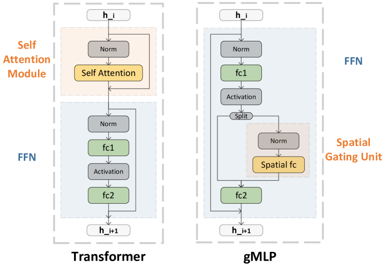
We compared the Transformer (Vaswani et al., 2017a) with the gMLP (Liu et al., 2021a) model architecture in Fig. 8. When comparing these two model structures, the FFN module is the same. The differences exist in the token-wise operations. The Transformer leverages the self attention module to calculate the relations between different tokens. However, the gMLP model leverages the Spatial Gating Unit to replace the self attention module.

Figure 8: Model architecture comparison: Transformer v.s. gMLP

Appendix E Downstream Task Descriptions

We evaluate on six representative tasks covering commonsense reasoning and question answering, including:

• COPA (Choice of Plausible Alternatives) (Roemmele et al., 2011) is a causal reasoning task in which a system is given a premise sentence and must determine either the cause or effect of the premise from two possible choices. All examples are handcrafted and focus on blogs and photography-related encyclopedia topics.

• PIQA (PhysicalQA) (Bisk et al., 2020) is a question answering task which asks common sense questions about how the physical world works and is intended as a probe of grounded understanding of the world.

• StoryCloze (Mostafazadeh et al., 2016) involves selecting the correct ending sentence for five-sentence long stories.

• Winogrande The Winograd Schemas Challenge (Levesque et al., 2012) is a classical task in NLP that involves determining which word a pronoun refers to when the pronoun is grammatically ambiguous but semantically unambiguous to a human. Recently fine-tuned language models have achieved near-human performance on the original Winograd dataset, but more complex versions adversarially-mined Winogrande dataset (Sakaguchi et al., 2020) still significantly lag human performance. We test our performance on Winogrande.

• HellaSwag dataset (Zellers et al., 2019) involves picking the best ending to a story or set of instructions. The examples were adversarially mined to be difficult for language models.

• ReCoRD (Reading Comprehension with Commonsense Reasoning Dataset) (Zhang et al., 2018) is a multiple-choice QA task. Each example consists of a news article and a Cloze-style question about the article in which one entity is masked out. The system must predict the masked out entity from a list of possible entities in the provided passage, where the same entity may be expressed with multiple different surface forms, which are all considered correct. Articles are from CNN and Daily Mail.

References

- Artetxe et al. (2021) Artetxe, M., Bhosale, S., Goyal, N., Mihaylov, T., Ott, M., Shleifer, S., Lin, X. V., Du, J., Iyer, S., Pasunuru, R., et al. Efficient large scale language modeling with mixtures of experts. arXiv preprint arXiv:2112.10684, 2021.
- Bertsekas (1992) Bertsekas, D. P. Auction algorithms for network flow problems: A tutorial introduction. Computational optimization and applications, 1(1):7–66, 1992.
- Bisk et al. (2020) Bisk, Y., Zellers, R., Gao, J., Choi, Y., et al. Piqa: Reasoning about physical commonsense in natural language. In Proceedings of the AAAI Conference on Artificial Intelligence, volume 34, pp. 7432–7439, 2020.
- Brown et al. (2020a) Brown, T. B., Mann, B., Ryder, N., Subbiah, M., Kaplan, J., Dhariwal, P., Neelakantan, A., Shyam, P., Sastry, G., Askell, A., et al. Language models are few-shot learners. arXiv preprint arXiv:2005.14165, 2020a.
- Brown et al. (2020b) Brown, T. B., Mann, B., Ryder, N., Subbiah, M., Kaplan, J., Dhariwal, P., Neelakantan, A., Shyam, P., Sastry, G., Askell, A., et al. Language models are few-shot learners. arXiv preprint arXiv:2005.14165, 2020b.
- Clark et al. (2022) Clark, A., Casas, D. d. l., Guy, A., Mensch, A., Paganini, M., Hoffmann, J., Damoc, B., Hechtman, B., Cai, T., Borgeaud, S., et al. Unified scaling laws for routed language models. arXiv preprint arXiv:2202.01169, 2022.
- Conneau et al. (2019) Conneau, A., Khandelwal, K., Goyal, N., Chaudhary, V., Wenzek, G., Guzmán, F., Grave, E., Ott, M., Zettlemoyer, L., and Stoyanov, V. Unsupervised cross-lingual representation learning at scale. arXiv preprint arXiv:1911.02116, 2019.
- Devlin et al. (2018) Devlin, J., Chang, M.-W., Lee, K., and Toutanova, K. Bert: Pre-training of deep bidirectional transformers for language understanding. arXiv preprint arXiv:1810.04805, 2018.
- Fedus et al. (2021) Fedus, W., Zoph, B., and Shazeer, N. Switch transformers: Scaling to trillion parameter models with simple and efficient sparsity. arXiv preprint arXiv:2101.03961, 2021.
- Gokaslan & Cohen (2019) Gokaslan, A. and Cohen, V. Openwebtext corpus. In http://web.archive.org/save/http://Skylion007.github.io/ OpenWebTextCorpus., 2019.
- Hochreiter & Schmidhuber (1997) Hochreiter, S. and Schmidhuber, J. Long short-term memory. Neural computation, 9(8):1735–1780, 1997.
- Hou et al. (2021) Hou, Q., Jiang, Z., Yuan, L., Cheng, M.-M., Yan, S., and Feng, J. Vision permutator: A permutable mlp-like architecture for visual recognition. arXiv preprint arXiv:2106.12368, 2021.
- Jaszczur et al. (2021) Jaszczur, S., Chowdhery, A., Mohiuddin, A., Kaiser, L., Gajewski, W., Michalewski, H., and Kanerva, J. Sparse is enough in scaling transformers. Advances in Neural Information Processing Systems, 34:9895–9907, 2021.
- Lee-Thorp et al. (2021) Lee-Thorp, J., Ainslie, J., Eckstein, I., and Ontanon, S. Fnet: Mixing tokens with fourier transforms. arXiv preprint arXiv:2105.03824, 2021.
- Lepikhin et al. (2020) Lepikhin, D., Lee, H., Xu, Y., Chen, D., Firat, O., Huang, Y., Krikun, M., Shazeer, N., and Chen, Z. Gshard: Scaling giant models with conditional computation and automatic sharding. arXiv preprint arXiv:2006.16668, 2020.
- Levesque et al. (2012) Levesque, H., Davis, E., and Morgenstern, L. The winograd schema challenge. In Thirteenth International Conference on the Principles of Knowledge Representation and Reasoning, 2012.
- Lewis et al. (2021) Lewis, M., Bhosale, S., Dettmers, T., Goyal, N., and Zettlemoyer, L. Base layers: Simplifying training of large, sparse models. arXiv preprint arXiv:2103.16716, 2021.
- Liu et al. (2021a) Liu, H., Dai, Z., So, D. R., and Le, Q. V. Pay attention to mlps. arXiv preprint arXiv:2105.08050, 2021a.
- Liu et al. (2021b) Liu, H., Dai, Z., So, D. R., and Le, Q. V. Pay attention to mlps. arXiv preprint arXiv:2105.08050, 2021b.
- Liu et al. (2019) Liu, Y., Ott, M., Goyal, N., Du, J., Joshi, M., Chen, D., Levy, O., Lewis, M., Zettlemoyer, L., and Stoyanov, V. Roberta: A robustly optimized bert pretraining approach. arXiv preprint arXiv:1907.11692, 2019.
- Lou et al. (2021) Lou, Y., Xue, F., Zheng, Z., and You, Y. Sparse-mlp: A fully-mlp architecture with conditional computation. arXiv preprint arXiv:2109.02008, 2021.
- Mostafazadeh et al. (2016) Mostafazadeh, N., Chambers, N., He, X., Parikh, D., Batra, D., Vanderwende, L., Kohli, P., and Allen, J. A corpus and evaluation framework for deeper understanding of commonsense stories. arXiv preprint arXiv:1604.01696, 2016.
- Nagel (2016) Nagel, S. Cc-news. In http://web.archive.org/save/http://commoncrawl.org /2016/10/newsdataset-available., 2016.
- Ott et al. (2019) Ott, M., Edunov, S., Baevski, A., Fan, A., Gross, S., Ng, N., Grangier, D., and Auli, M. fairseq: A fast, extensible toolkit for sequence modeling. arXiv preprint arXiv:1904.01038, 2019.
- Paszke et al. (2017) Paszke, A., Gross, S., Chintala, S., Chanan, G., Yang, E., DeVito, Z., Lin, Z., Desmaison, A., Antiga, L., and Lerer, A. Automatic differentiation in pytorch. 2017.
- Radford et al. (2018) Radford, A., Narasimhan, K., Salimans, T., and Sutskever, I. Improving language understanding by generative pre-training. 2018.
- Radford et al. (2019) Radford, A., Wu, J., Child, R., Luan, D., Amodei, D., Sutskever, I., et al. Language models are unsupervised multitask learners. OpenAI blog, 1(8):9, 2019.
- Raffel et al. (2019) Raffel, C., Shazeer, N., Roberts, A., Lee, K., Narang, S., Matena, M., Zhou, Y., Li, W., and Liu, P. J. Exploring the limits of transfer learning with a unified text-to-text transformer. arXiv preprint arXiv:1910.10683, 2019.
- Riquelme et al. (2021) Riquelme, C., Puigcerver, J., Mustafa, B., Neumann, M., Jenatton, R., Pinto, A. S., Keysers, D., and Houlsby, N. Scaling vision with sparse mixture of experts. arXiv preprint arXiv:2106.05974, 2021.
- Roemmele et al. (2011) Roemmele, M., Bejan, C. A., and Gordon, A. S. Choice of plausible alternatives: An evaluation of commonsense causal reasoning. In 2011 AAAI Spring Symposium Series, 2011.
- Roller et al. (2021) Roller, S., Sukhbaatar, S., Szlam, A., and Weston, J. Hash layers for large sparse models. arXiv preprint arXiv:2106.04426, 2021.
- Sakaguchi et al. (2020) Sakaguchi, K., Le Bras, R., Bhagavatula, C., and Choi, Y. Winogrande: An adversarial winograd schema challenge at scale. In Proceedings of the AAAI Conference on Artificial Intelligence, volume 34, pp. 8732–8740, 2020.
- Shazeer et al. (2017) Shazeer, N., Mirhoseini, A., Maziarz, K., Davis, A., Le, Q., Hinton, G., and Dean, J. Outrageously large neural networks: The sparsely-gated mixture-of-experts layer. arXiv preprint arXiv:1701.06538, 2017.
- Tolstikhin et al. (2021) Tolstikhin, I., Houlsby, N., Kolesnikov, A., Beyer, L., Zhai, X., Unterthiner, T., Yung, J., Keysers, D., Uszkoreit, J., Lucic, M., et al. Mlp-mixer: An all-mlp architecture for vision. arXiv preprint arXiv:2105.01601, 2021.
- Trinh & Le (2018) Trinh, T. H. and Le, Q. V. A simple method for commonsense reasoning. arXiv preprint arXiv:1806.02847, 2018.
- Vaswani et al. (2017a) Vaswani, A., Shazeer, N., Parmar, N., Uszkoreit, J., Jones, L., Gomez, A. N., Kaiser, L., and Polosukhin, I. Attention is all you need. arXiv preprint arXiv:1706.03762, 2017a.
- Vaswani et al. (2017b) Vaswani, A., Shazeer, N., Parmar, N., Uszkoreit, J., Jones, L., Gomez, A. N., Kaiser, Ł., and Polosukhin, I. Attention is all you need. In Advances in neural information processing systems, pp. 5998–6008, 2017b.
- Yang et al. (2021) Yang, A., Lin, J., Men, R., Zhou, C., Jiang, L., Jia, X., Wang, A., Zhang, J., Wang, J., Li, Y., et al. Exploring sparse expert models and beyond. arXiv preprint arXiv:2105.15082, 2021.
- Zellers et al. (2019) Zellers, R., Holtzman, A., Bisk, Y., Farhadi, A., and Choi, Y. Hellaswag: Can a machine really finish your sentence? arXiv preprint arXiv:1905.07830, 2019.
- Zhang et al. (2018) Zhang, S., Liu, X., Liu, J., Gao, J., Duh, K., and Van Durme, B. Record: Bridging the gap between human and machine commonsense reading comprehension. arXiv preprint arXiv:1810.12885, 2018.
- Zhu et al. (2015) Zhu, Y., Kiros, R., Zemel, R., Salakhutdinov, R., Urtasun, R., Torralba, A., and Fidler, S. Aligning books and movies: Towards story-like visual explanations by watching movies and reading books. In Proceedings of the IEEE international conference on computer vision, pp. 19–27, 2015.
- Zoph et al. (2022) Zoph, B., Bello, I., Kumar, S., Du, N., Huang, Y., Dean, J., Shazeer, N., and Fedus, W. Designing effective sparse expert models. arXiv preprint arXiv:2202.08906, 2022.