ADAS: A Direct Adaptation Strategy for Multi-Target Domain Adaptive Semantic Segmentation

Abstract

In this paper, we present a direct adaptation strategy (ADAS), which aims to directly adapt a single model to multiple target domains in a semantic segmentation task without pretrained domain-specific models. To do so, we design a multi-target domain transfer network (MTDT-Net) that aligns visual attributes across domains by transferring the domain distinctive features through a new target adaptive denormalization (TAD) module. Moreover, we propose a bi-directional adaptive region selection (BARS) that reduces the attribute ambiguity among the class labels by adaptively selecting the regions with consistent feature statistics. We show that our single MTDT-Net can synthesize visually pleasing domain transferred images with complex driving datasets, and BARS effectively filters out the unnecessary region of training images for each target domain. With the collaboration of MTDT-Net and BARS, our ADAS achieves state-of-the-art performance for multi-target domain adaptation (MTDA). To the best of our knowledge, our method is the first MTDA method that directly adapts to multiple domains in semantic segmentation.

Figure 1: Multi-target domain transfer results of our single MTDT-Net in the driving scenes. The top row and leftmost column represent source domain images and multiple target domain images, respectively. The other images are the domain transferred images generated by passing the source image at each column through our MTDT-Net.

1 Introduction

Unsupervised domain adaptation (UDA)[26, 49, 14, 20, 27] aims to alleviate the performance drop caused by the distribution discrepancy between domains. It is widely utilized in synthetic-to-real adaptation for various computer vision applications that require a large number of labeled data. Most of the works are designed for single-target domain adaptation (STDA), which allows a single network to adapt to a specific target domain. It rarely addresses the variability in the real-world, particularly changes in driving region, illumination, and weather conditions in autonomous driving scenarios. This issue can be tackled by adopting multiple target-specific adaptation models, but this limits the memory efficiency, scalability, and practical utility of embedded autonomous systems.

Recently, multi-target domain adaptation (MTDA) methods [58, 43, 11, 40, 18, 48] have been proposed, which enables a single model to adapt a labeled source domain to multiple unlabeled target domains. Most of works train multiple STDA models and then distill the knowledge into a single multi-target domain adaptation network. Recent approaches[40, 18, 48] transfer the knowledge from label predictors as shown in Fig. 2-(a). These methods show impressive results, but their performance can be restricted by the performance of the pretrained models. Moreover, inaccurate label predictions in the teacher network can degrade model performance, but none of works have deeply investigated them. To address this problem, we propose A Direct Adaptation Strategy (ADAS) that directly adapts a single model to multiple target domains without pretrained STDA models, as shown in Fig. 2-(b). Our approach achieves robust multi-domain adaptation by exploiting the feature statistics of training data on multiple domains. The followings provides a detailed introduction of our sub-modules: Multi-Target Domain Transfer Networks (MTDT-Net) and a Bi-directional Adaptive Region Selection (BARS).

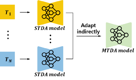
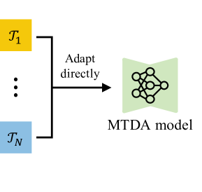
(a) Existing MTDA method		(b) Ours

Figure 2: Illustration of the existing MTDA and our method. (a) Conventional MTDA methods pretrain each STDA model then distill the knowledge into a single MTDA model. (b) Our ADAS directly adapts multiple target domains.

MTDT-Net We present a Multi-Target Domain Transfer Network (MTDT-Net) that transfers the distinctive attribute of target domains to a source domain rather than learning all of the target domain distributions. Our network consists of a novel Target Adaptive Denormalization (TAD) that helps to adapt the statistics of source feature to that of the target feature. While the existing works on UDA [31, 3, 37, 14, 6, 7, 34] require domain-specific encoders and generators for multi-target domain adaptation, the TAD module enables our single network to adapt to multiple domains. Fig. ADAS: A Direct Adaptation Strategy for Multi-Target Domain Adaptive Semantic Segmentation shows how a single MTDT-Net can efficiently synthesize visually pleasing domain transferred images.

GTA5 $\to$ Cityscapes	Cityscapes
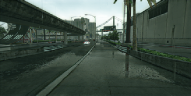
(a) Domain transferred image	(b) Target image
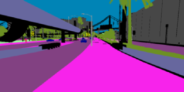
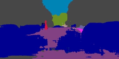
(c) Ground-truth label of (a)	(d) Pseudo label of (b)
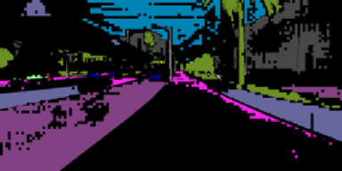
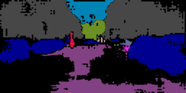
(e) Selected region of (c)	(f) Selected region of (d)

Figure 3: Examples of the regions with similar attributes but different labels (c) (purple: road, pink: sidewalk), and the noisy prediction (d). The black regions in (e) and (f) are regions filtered by BARS.

BARS Although the visual attributes across domains are well-aligned, there are still some attribute ambiguities among the class labels in semantic segmentation. The ambiguity is usually observed on the regions with similar attributes but different label, such as the sidewalks in GTA5 and the roads in Cityscapes as shown in Fig. 3-(a),(c). This confuses the model finding the accurate decision boundary. Moreover, the predictions from target domains usually have noisy labels leading to inaccurate training of the task network, as shown in Fig. 3-(b),(d). To solve these issues, we propose a Bi-directional Adaptive Region Selection (BARS), which alleviates the confusion. It adaptively selects the regions with consistent feature statistics as shown in Fig. 3-(e). It can also select the pseudo label of the target images for our self-training scheme, as shown in Fig. 3-(f). We show that BARS allows the task network to perform robust training and achieve the improved performance.

To the best of our knowledge, our multi-target domain adaptation method is the first approach that directly adapts the task network to multiple target domains without pretrained STDA models in semantic segmentation. The extensive experiments show that the proposed method achieves state-of-the-art performance on semantic segmentation task. At the end, we demonstrate the effectiveness of the proposed MTDT-Net and BARS.

2 Related Work

2.1 Domain Transfer

With the advent of generative adversarial networks (GANs)[12], the adversarial learning has shown promising results not only in photorealistic image synthesis[44, 1, 36, 35, 22, 23, 4, 24] but also in domain transfer[19, 61, 29, 51, 17, 26, 30, 49, 14, 20, 27]. The traditional domain transfer methods rely on adversarial learning[19, 61, 29, 51] or the typical style transfer method[10, 53, 9, 38, 16]. Afterwards, the studies on feature disentanglement [17, 26, 30, 42, 27] present a model that can apply various styles by appropriately utilizing disentangled features that are separately encoded as content and style. Recent works[46, 62] have tackled more in-depth domain transfer problems. Richter et al. [46] propose a rendering-aware denormalization (RAD) that constructs style tensors by using the abundant condition information from G-buffers, and show high fidelity domain transfer in a driving scene. Zhu et al. [62] propose a semantic region-wise domain transfer model by extracting a style vector for each semantic region.

2.2 Unsupervised Domain Adaptation for Semantic Segmentation

Traditional feature-level adaptation methods [15, 32, 33, 52, 55] aim to align the source and target distribution in feature space. Most of them [15, 32, 33] adopt adversarial learning with the intermediate features of the segmentation network, and the others [52, 55] directly apply adversarial loss to output prediction. Pixel-level adaptation methods[31, 3, 37, 27] reduce the domain gap in the image-level by synthesizing target-styled images. Several works [14, 7, 6] adopt both feature-level and pixel-level methods. Another direction of UDA [63, 60, 28, 34, 59] is to take a self-supervised learning approach for dense prediction tasks, such as semantic segmentation. Some works [63, 60, 28] obtain high confidence labels measured by the uncertainty of target prediction, and use them as pseudo ground-truth. The others [34, 59] use proxy features by extracting the centroid of the intermediate features of each class to remove uncertain regions in the pseudo-label.

2.3 Multi-Target Domain Adaptation

Early studies on MTDA have tackled classification tasks using adaptive learning of a common model parameter dictionary [58], domain-invariant feature extraction [43], or knowledge distillation [40]. Recently, using MTDA on more high-level vision tasks such as semantic segmentation [18, 48] has become an interesting and challenging research topic. These works employ knowledge distillation to transfer the knowledge of domain specific teacher models to a domain-agnostic student model. For more robust adaptation, Isobe et al. [18] enforce the weight regularization to the student network and Saporta et al. [48] use a shared feature extractor that constructs a common feature space for all domains. In this work, we present a more efficient and simpler method that handles multiple domains using a unified architecture without teacher networks or weight regularization.

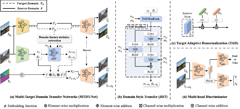
Figure 4: Overview of the proposed MTDT-Net. (a) MTDT-Net consists of an encoder $E$, a style encoder $SE$, a domain style transfer network $DST$ and a generator $G$. Given a source image, label map $I_{\mathcal{S}},Y_{\mathcal{S}}$, and target images $I_{\mathcal{T}_{k}}$, MTDT-Net aims to produce domain transferred image $I_{\mathcal{S}\to\mathcal{T}_{k}}$. The other reconstructed images $I^{\prime}_{\mathcal{S}},I^{\prime}_{\mathcal{T}_{k}},I^{\prime\prime}_{\mathcal{S}}$ are auxiliary outputs generated only during the training process. (b) $DST$ consists of two TAD residual blocks (ResBlock). The TAD module is followed by each convolutional layer, given the channel-wise statistics of target domains $\mu_{\mathcal{T}_{k}},\sigma_{\mathcal{T}_{k}}$. (c) TAD transfers the target domain with $\mu_{\mathcal{T}_{k}},\sigma_{\mathcal{T}_{k}}$ by statistics modulation. (d) The multi-head discriminator predicts which domain the image is from, as well as determines whether the image is real or fake. Note that, for the sake of brevity, we illustrate a single target domain setting, but our model deals with multi-target domain adaptation.

3 A Direct Adaptation Strategy (ADAS)

In this section, we describe our direct adaptation strategy for multi-target domain adaptive semantic segmentation. We have a labeled source dataset $\mathcal{S}=\{I_{\mathcal{S}},Y_{\mathcal{S}}\}$ and $N$ unlabeled target datasets $\mathcal{T}_{k}=\{I_{\mathcal{T}_{k}}\},k\in\{1,...,N\}$, where $I$ and $Y$ are the image and the ground-truth label, respectively. The goal of our approach is to directly adapt a segmentation network $T$ to multiple target domains without training STDA models. Our strategy contains two sub-modules: a multi-target domain transfer network (MTDT-Net), and a bi-directional adaptive region selection (BARS). We describe the details of MTDT-Net and BARS in Sec. 3.1 and Sec. 3.2, respectively.

3.1 Multi-Target Domain Transfer Network (MTDT-Net)

The overall pipeline of MTDT-Net is illustrated in Fig. 4-(a). The network consists of an encoder $E$, a generator $G$, a style extractor $SE$, a domain style transfer network $DST$. To build an image feature space, we adopt a typical autoencoder structure with the encoder $E$ and the generator $G$. Given the source and target images $I_{\mathcal{S}},I_{\mathcal{T}_{1}},...,I_{\mathcal{T}_{N}}$, the encoder $E$ extracts the individual features $\mathcal{F}_{\mathcal{S}},\mathcal{F}_{\mathcal{T}_{1}},...\mathcal{F}_{\mathcal{T}_{N}}$ that are later passed through the generator $G$ to reconstruct the original input images $I^{\prime}_{\mathcal{S}},I^{\prime}_{\mathcal{T}_{1}},...,I^{\prime}_{\mathcal{T}_{N}}$ as follows:

$$\begin{split}\mathcal{F}_{\mathcal{S}}=E(I_{\mathcal{S}}),~{}~{}\mathcal{F}_{\mathcal{T}_{k}}=E(I_{\mathcal{T}_{k}}),\\ I^{\prime}_{\mathcal{S}}=G(\mathcal{F}_{\mathcal{S}}),~{}~{}I^{\prime}_{\mathcal{T}_{k}}=G(\mathcal{F}_{\mathcal{T}_{k}}).\end{split}$$ (1)

We extract the style tensors $\gamma_{\mathcal{S}}$, $\beta_{\mathcal{S}}$ of the source image through the style encoder $SE$, and the content tensor $\mathcal{C}_{\mathcal{S}}$ from the segmentation label only in the source domain through an $1\times 1$ convolutional layer $\phi(\cdot)$ as follows:

$$\begin{split}\{\gamma_{\mathcal{S}},\beta_{\mathcal{S}}\}=SE(I_{\mathcal{S}}),~{}\mathcal{C_{S}}=\phi(Y_{\mathcal{S}}).\end{split}$$ (2)

We assume that the image features are composed of the scene structure and detail representation, which we call the content feature $\mathcal{C}_{\mathcal{S}}$ and style feature $\gamma_{\mathcal{S}}$, $\beta_{\mathcal{S}}$ as follows:

$$\begin{split}I^{\prime\prime}_{\mathcal{S}}=G(\mathcal{F}^{\prime}_{\mathcal{S}}),~{}\mathcal{F}^{\prime}_{\mathcal{S}}=\gamma_{\mathcal{S}}\mathcal{C_{S}}+\beta_{\mathcal{S}},\end{split}$$ (3)

where the source image feature $\mathcal{F}^{\prime}_{\mathcal{S}}$ is passed through generator $G$ to obtain the reconstructed input image $I^{\prime\prime}_{\mathcal{S}}$. The synthesized images $I^{\prime}_{\mathcal{S}},I^{\prime}_{\mathcal{T}_{k}},I^{\prime\prime}_{\mathcal{S}}$ are auxiliary outputs to be utilized for network training. The goal of our network is to generate a domain transferred image $I_{\mathcal{S}\to{\mathcal{T}_{k}}}$ using the same generator $G$ as follows:

$$\begin{split}I_{\mathcal{S}\to{\mathcal{T}_{k}}}=G(\mathcal{F}_{\mathcal{S}\to{\mathcal{T}_{k}}}),~{}\mathcal{F}_{\mathcal{S}\to{\mathcal{T}_{k}}}=\gamma_{\mathcal{S}\to{\mathcal{T}_{k}}}\mathcal{C_{S}}+\beta_{\mathcal{S}\to{\mathcal{T}_{k}}},\end{split}$$ (4)

where $\mathcal{F}_{\mathcal{S}\to{\mathcal{T}_{k}}}$ is the domain transferred features, which is composed of the source content $\mathcal{C_{S}}$ and the $k$-th target domain style features $\gamma_{\mathcal{S}\to{\mathcal{T}_{k}}},\beta_{\mathcal{S}\to{\mathcal{T}_{k}}}$.

To obtain the target domain style tensors, we design a domain style transfer network ($DST$) which transfers the source style tensors $\gamma_{\mathcal{S}},\beta_{\mathcal{S}}$ to the target style tensors $\gamma_{\mathcal{S}\to\mathcal{T}_{k}},\beta_{\mathcal{S}\to\mathcal{T}_{k}}$ as follows:

$$\begin{split}\gamma_{\mathcal{S}\to{\mathcal{T}_{k}}},\beta_{\mathcal{S}\to{\mathcal{T}_{k}}}=DST(\gamma_{\mathcal{S}},\beta_{\mathcal{S}},\mu_{\mathcal{T}_{k}},\sigma_{\mathcal{T}_{k}}),\end{split}$$ (5)

where the channel-wise mean $\mu_{\mathcal{T}_{k}}$ and variance $(\sigma_{\mathcal{T}_{k}})^{2}$ vectors encode the $k$-th target domain feature statistics computed by the cumulative moving average (CMA) algorithm and Welford’s online algorithm [56] described in Alg. 1. The $DST$ in Fig. 4-(b) consists of two TAD ResBlock built with a series of convolutional layer, our new Target-Adaptive Denormalization (TAD), and ReLU. TAD is a conditional normalization module that modulates the normalized input with learned scale and bias similar to SPADE[41] and RAD[46] as shown in Fig. 4-(c). We pass the standard deviation $\sigma_{\mathcal{T}_{k}}$ and the target mean $\mu_{\mathcal{T}_{k}}$ through each fully connected (FC) layer and use them as scale and bias as follows:

$$\begin{split}\text{TAD}(\hat{f}_{\mathcal{S}},\mu_{\mathcal{T}_{k}},\sigma_{\mathcal{T}_{k}})=FC(\sigma_{\mathcal{T}_{k}})\hat{f}_{\mathcal{S}}+FC(\mu_{\mathcal{T}_{k}}),\end{split}$$ (6)

where $\hat{f}_{\mathcal{S}}$ is the instance-normalized [53] input to TAD. For adversarial learning with multiple target domains, we adopt a multi-head discriminator composed of an adversarial discriminator $D_{adv}=D^{\prime}_{adv}\circ D_{shared}$ and a domain classifier $D_{cls}=D^{\prime}_{cls}\circ D_{shared}$ as shown in Fig. 4-(d).

Each group of networks $\mathcal{G}=\{E,SE,DST,G,\phi\}$ and $\mathcal{D}=\{D_{adv},D_{cls}\}$ is trained by minimizing the following losses, $\mathcal{L}^{\mathcal{G}}$ and $\mathcal{L}^{\mathcal{D}}$, respectively:

$$\begin{split}\mathcal{L}^{\mathcal{D}}=-\mathcal{L}_{adv}+\mathcal{L}_{cls}^{\mathcal{D}},\\ \mathcal{L}^{\mathcal{G}}=\mathcal{L}_{rec}+\mathcal{L}_{per}+\mathcal{L}_{adv}+\mathcal{L}_{cls}^{\mathcal{G}}.\end{split}$$ (7)

Reconstruction Loss We impose L1 loss on the reconstructed images $I^{\prime}_{\mathcal{S}},I^{\prime}_{\mathcal{T}_{k}},I^{\prime\prime}_{\mathcal{S}}$ to build an image feature space:

$$\begin{split}\mathcal{L}_{rec}=\mathcal{L}_{1}(I_{\mathcal{S}},I^{\prime}_{\mathcal{S}})+\mathcal{L}_{1}(I_{\mathcal{S}},I^{\prime\prime}_{\mathcal{S}})+\sum_{k=1}^{N}\mathcal{L}_{1}(I_{\mathcal{T}_{k}},I^{\prime}_{\mathcal{T}_{k}}).\end{split}$$ (8)

Adversarial Loss We apply the patchGAN [19] discriminator $D_{adv}$ to impose an adversarial loss on the domain transferred images and the corresponding target images:

$$\begin{split}\mathcal{L}_{adv}&=\sum_{k=1}^{N}\Big{(}\mathbb{E}_{I_{\mathcal{T}_{k}}}\left[\log D_{adv}(I_{\mathcal{T}_{k}})\right]\\ &+\mathbb{E}_{I_{\mathcal{S}\to{\mathcal{T}_{k}}}}\left[1-\log D_{adv}(I_{\mathcal{S}\to{\mathcal{T}_{k}}})\right]\Big{)}.\\ \end{split}$$ (9)

Algorithm 1 Domain feature statistics extraction

0:  $\mathcal{F}_{\mathcal{T}_{k}}\in\mathbb{R}^{H\times W\times C},k\in\{1,...,N\}$

0:  $\mu_{\mathcal{T}_{k}},(\sigma_{\mathcal{T}_{k}})^{2}\in\mathbb{R}^{C}$ % 1. Initialization

1:  for $k=1~{}to~{}N$ do

2:     $M_{\mathcal{T}_{k}}=0$, $S_{\mathcal{T}_{k}}=0$ //$M_{\mathcal{T}_{k}},S_{\mathcal{T}_{k}}\in\mathbb{R}^{H\times W\times C}$

3:  end for% 2. Online update //$N_{update}$ is # of update iterations

4:  for $n=0~{}to~{}{N_{update}}$ do

5:     for $k=1~{}to~{}N$ do

6:        $\mu_{n}^{\mathcal{T}_{k}}\xleftarrow{}\frac{1}{HW}\sum_{i=0}^{H-1}\sum_{j=0}^{W-1}{M_{\mathcal{T}_{k}}{(i,j)}}$

7:        $M_{\mathcal{T}_{k}}\xleftarrow{}M_{\mathcal{T}_{k}}+({{\mathcal{F}_{\mathcal{T}_{k}}-M_{\mathcal{T}_{k}}})/({n+1})}$

8:        $\mu_{n+1}^{\mathcal{T}_{k}}\xleftarrow{}\frac{1}{HW}\sum_{i=0}^{H-1}\sum_{j=0}^{W-1}{M_{\mathcal{T}_{k}}(i,j)}$

9:        ${\tilde{\mu}}_{n}^{\mathcal{T}_{k}},{\tilde{\mu}}_{n+1}^{\mathcal{T}_{k}}$ $\leftarrow{}$ expand $\mu_{n}^{\mathcal{T}_{k}},\mu_{n+1}^{\mathcal{T}_{k}}$ to $\mathbb{R}^{H\times W\times C}$

10:        if $n=0$ then

11:           $S_{\mathcal{T}_{k}}\xleftarrow{}(\mathcal{F}_{\mathcal{T}_{k}}-{\tilde{\mu}}_{n+1}^{\mathcal{T}_{k}})^{2}$

12:        else

13:           $S_{\mathcal{T}_{k}}\xleftarrow{}S_{\mathcal{T}_{k}}+(\mathcal{F}_{\mathcal{T}_{k}}-{\tilde{\mu}}_{n}^{\mathcal{T}_{k}})(\mathcal{F}_{\mathcal{T}_{k}}-{\tilde{\mu}}_{n+1}^{\mathcal{T}_{k}})$

14:           $\mu_{\mathcal{T}_{k}}\xleftarrow{}\mu^{\mathcal{T}_{k}}_{n+1}$

15:           $(\sigma_{\mathcal{T}_{k}})^{2}\xleftarrow{}\frac{1}{nHW}\sum_{i=0}^{H-1}\sum_{j=0}^{W-1}{S_{\mathcal{T}_{k}}(i,j)}$

16:        end if

17:     end for

18:  end for

Domain Classification Loss We build the domain classifier $D_{cls}$ to classify the domain of the input images. We impose the cross-entropy loss with the target images for $\mathcal{D}$ and with the domain transferred images for $\mathcal{G}$:

$$\begin{split}\mathcal{L}_{cls}^{\mathcal{D}}&=-\sum_{k=1}^{N}t_{k}\log D_{cls}(I_{\mathcal{T}_{k}}),\\ \mathcal{L}_{cls}^{\mathcal{G}}&=-\sum_{k=1}^{N}t_{k}\log D_{cls}(I_{\mathcal{S}\to{\mathcal{T}_{k}}}),\end{split}$$ (10)

where $t_{k}\in\mathbb{R}^{N}$ is the one-hot encoded class label of the target domain $\mathcal{T}_{k}$.

Perceptual Loss We impose a perceptual loss [21] widely used for domain transfer as well as style transfer [9, 16]:

$$\begin{split}\mathcal{L}_{per}=\sum_{k=1}^{N}\sum_{l\in L}||P_{l}(I_{\mathcal{S}})-P_{l}(I_{\mathcal{S}\to{\mathcal{T}_{k}}})||_{2}^{2},\end{split}$$ (11)

where the set of layers $L$ is the subset of the perceptual network $P$.

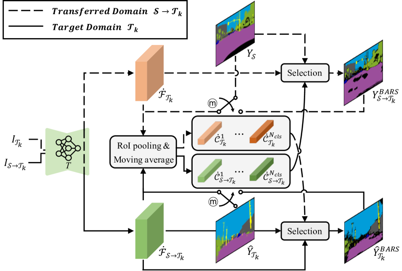
Figure 5: Overview of BARS. For each class $c\in\{1,...,N_{cls}\}$, BARS extracts the centroids $\dot{\mathcal{C}}^{c}_{\mathcal{S}\to{\mathcal{T}_{k}}},\dot{\mathcal{C}}^{c}_{\mathcal{T}_{k}}$ from the intermediate features $\dot{\mathcal{F}}_{\mathcal{S}\to{\mathcal{T}_{k}}},\dot{\mathcal{F}}_{\mathcal{T}_{k}}$ of the segmentation network $T$ with RoI pooling and update them with CMA algorithm. Then, BARS measures the similarity of two cases, “$\dot{\mathcal{F}}_{\mathcal{S}\to{\mathcal{T}_{k}}}\leftrightarrow\dot{\mathcal{C}}_{\mathcal{T}_{k}}^{c}$” and “$\dot{\mathcal{F}}_{\mathcal{T}_{k}}\leftrightarrow\dot{\mathcal{C}}_{\mathcal{S}\to{\mathcal{T}_{k}}}^{c}$”, and selects the adaptive region. ⓜ is a switch that selects the labels for centroid update in Equ. (12), either $Y_{\mathcal{S}}$, $\hat{Y}_{\mathcal{T}_{k}}$ for the first $m$ iterations or $Y^{BARS}_{\mathcal{S}\to{\mathcal{T}_{k}}}$, $\hat{Y}^{BARS}_{\mathcal{T}_{k}}$ after the $m$ iterations. We set m as 300 iterations for our experiments.

	Method	Target	flat	constr.	object	nature	sky	human	vehicle	mIoU	Avg.
G $\to$C, I	ADVENT [55]	C	93.9	80.2	26.2	79.0	80.5	52.5	78.0	70.0	67.4
		I	91.8	54.5	14.4	76.8	90.3	47.5	78.3	64.8
	MTKT[48]	C	94.5	82.0	23.7	80.1	84.0	51.0	77.6	70.4	68.2
		I	91.4	56.6	13.2	77.3	91.4	51.4	79.9	65.9
	Ours	C	95.1	82.6	39.8	84.6	81.2	63.6	80.7	75.4	71.2
		I	90.5	63.0	22.2	73.7	87.9	54.3	76.9	66.9
1-122.5 G $\to$C, M	ADVENT[55]	C	93.1	80.5	24.0	77.9	81.0	52.5	75.0	69.1	68.9
		M	90.0	71.3	31.1	73.0	92.6	46.6	76.6	68.7
	MTKT[48]	C	95.0	81.6	23.6	80.1	83.6	53.7	79.8	71.1	70.9
		M	90.6	73.3	31.0	75.3	94.5	52.2	79.8	70.8
	Ours	C	96.4	83.5	35.1	83.8	84.9	62.3	81.3	75.3	73.9
		M	88.6	73.7	41.0	75.4	93.4	58.5	77.2	72.6
1-122.5 G $\to$C, I, M	ADVENT[55]	C	93.6	80.6	26.4	78.1	81.5	51.9	76.4	69.8	67.8
		I	92.0	54.6	15.7	77.2	90.5	50.8	78.6	65.6
		M	89.2	72.4	32.4	73.0	92.7	41.6	74.9	68.0
	MTKT[48]	C	94.6	80.7	23.8	79.0	84.5	51.0	79.2	70.4	69.1
		I	91.7	55.6	14.5	78.0	92.6	49.8	79.4	65.9
		M	90.5	73.7	32.5	75.5	94.3	51.2	80.2	71.1
	Ours	C	95.8	82.4	38.3	82.4	85.0	60.5	80.2	74.9	71.3
		I	89.9	52.7	25.0	78.1	92.1	51.0	77.9	66.7
		M	89.2	71.5	45.2	75.8	92.3	56.1	75.4	72.2

Table 1: Quantitative comparison between our method and state-of-the-art methods on GTA5 (G) to Cityscapes (C), IDD (I), and Mapilary (M) with 7 classes setting. Bold: Best score among all the methods.

3.2 Bi-directional Adaptive Region Selection (BARS)

The key idea of BARS is to select the pixels where the feature statistics are consistent, then train a task network $T$ by imposing loss on the selected region as illustrated in Fig. 5. We apply it in both the domain transferred image and the target image. We first extract each centroid feature $\dot{\mathcal{C}}$ of class $c$ as follows:

$$\begin{split}\dot{\mathcal{C}}_{\mathcal{S}\to\mathcal{T}_{k}}^{c}=\frac{1}{N_{c}}\sum_{i}\sum_{j}{\mathbbm{1}(Y_{\mathcal{S}}(i,j)=c)}\dot{\mathcal{F}}_{\mathcal{S}\to\mathcal{T}_{k}}(i,j),\\ \dot{\mathcal{C}}_{\mathcal{T}_{k}}^{c}=\frac{1}{N_{c}}\sum_{i}\sum_{j}{\mathbbm{1}(\hat{Y}_{\mathcal{T}_{k}}(i,j)=c)}\dot{\mathcal{F}}_{\mathcal{T}_{k}}(i,j),\end{split}$$ (12)

where $\mathbbm{1}$ is an indicator function, $N_{c}$ is the number of pixels of class $c$, and $i,j$ are the indices of the spatial coordinates. The feature map $\dot{\mathcal{F}}$ is from the second last layer of the task network $T$. To extract the centroids, we use the ground-truth label $Y_{\mathcal{S}}$ of the domain transferred image and the pseudo label $\hat{Y}_{\mathcal{T}_{k}}$ of the target image. For the online learning with the centroids, we also apply the CMA algorithm in Alg. 1 to the above centroids. Then, we design the selection mechanism using the following two assumptions:

• The region with features $\dot{\mathcal{F}}_{\mathcal{S}\to\mathcal{T}_{k}}$ far from the target centroid $\dot{\mathcal{C}}_{\mathcal{T}_{k}}$ would disturb the adaptation process.

• The region with target features $\dot{\mathcal{F}}_{\mathcal{T}_{k}}$ far from the centroids $\dot{\mathcal{C}}_{S\to\mathcal{T}_{k}}$ is likely to be a noisy prediction region.

Based on these assumptions, we find the nearest class $\dot{c}$ for each pixel in the feature map using the L2 distance between features on each pixels and centroid features as follows:

$$\begin{split}\dot{c}_{\mathcal{S}\to\mathcal{T}_{k}}(i,j)=\operatorname*{argmin}_{c}||\dot{\mathcal{F}}_{\mathcal{S}\to\mathcal{T}_{k}}(i,j)-\dot{\mathcal{C}}^{c}_{\mathcal{T}_{k}}||_{2},\\ \dot{c}_{\mathcal{T}_{k}}(i,j)=\operatorname*{argmin}_{c}||\dot{\mathcal{F}}_{\mathcal{T}_{k}}(i,j)-\dot{\mathcal{C}}_{\mathcal{S}\to\mathcal{T}_{k}}^{c}||_{2}.\end{split}$$ (13)

We obtain the filtered labels $Y_{\mathcal{S}\to{\mathcal{T}_{k}}}^{BARS}$, $\hat{Y}_{\mathcal{T}_{k}}^{BARS}$ using the nearest class $\dot{c}$:

$$\begin{split}Y_{\mathcal{S}\to{\mathcal{T}_{k}}}^{BARS}(i,j)=\begin{cases}Y_{\mathcal{S}}(i,j)&\quad\text{if}~{}\dot{c}_{\mathcal{S}\to\mathcal{T}_{k}}(i,j)=Y_{\mathcal{S}}(i,j),\\ \emptyset&\quad\text{otherwise}\\ \end{cases},\\ \hat{Y}_{\mathcal{T}_{k}}^{BARS}(i,j)=\begin{cases}\hat{Y}_{\mathcal{T}_{k}}(i,j)&\quad\text{if}~{}\dot{c}_{\mathcal{T}_{k}}(i,j)=\hat{Y}_{\mathcal{T}_{k}}(i,j),\\ \emptyset&\quad\text{otherwise}\\ \end{cases}.\end{split}$$ (14)

Finally, we train the task network $T$ with the labels using a typical cross-entropy loss $\mathcal{L}_{Task}$:

$$\begin{split}\min_{T}\left(\mathcal{L}_{Task}(I_{\mathcal{S}\to\mathcal{T}_{k}},Y_{\mathcal{S}\to{\mathcal{T}_{k}}}^{BARS})+\mathcal{L}_{Task}(I_{\mathcal{T}_{k}},\hat{Y}_{\mathcal{T}_{k}}^{BARS})\right).\end{split}$$ (15)

		7 classes			19 classes
	Image	GT	Source only	Ours	GT	Source only	Ours
C
I
M

Figure 6: Qualitative comparison between source only and our method on GTA5 (G) to Cityscapes (C), IDD (I), and Mapillary (M) with 7 classes and 19 classes setting.

4 Experiments

In this section, we describe the implementation details and experimental results of the proposed ADAS. We evaluate our method on a semantic segmentation task in both the synthetic-to-real adaptation in Sec. 4.2 and the real-to-real adaptation in Sec. 4.3 with multiple target domain datasets. We also conduct an extensive study to validate each submodule, MTDT-Net and BARS, in Sec. 4.4.

	Method	mIoU			mIoU
		C	I	M	Avg.
G$\to$C, I	CCL[18]	45.0	46.0	-	45.5
	Ours	45.8	46.3	-	46.1
G$\to$C, M	CCL[18]	45.1	-	48.8	46.8
	Ours	45.8	-	49.2	47.5
G$\to$I, M	CCL[18]	-	44.5	46.4	45.5
	Ours	-	46.1	47.6	46.9
G$\to$C, I, M	CCL[18]	46.7	47.0	49.9	47.9
	Ours	46.9	47.7	51.1	48.6

Table 2: Results of adapting GTA5 to Cityscapes (C), IDD (I), and Mapillary (M) with 19 classes setting.

4.1 Training Details

Datasets We use four different driving datasets containing one synthetic and three real-world datasets, each of which has a unique scene structure and visual appearance.

• GTA5[47] is a synthetic dataset of 24,966 labeled images captured from a video game.

• Cityscapes[8] is an urban dataset collected from European cities, and includes 2,975 images in the training set and 500 in the validation set.

• IDD[54] has total 10,003 Indian urban driving scenes, which contains 6,993 images for training, 981 for validation and 2,029 for test.

• Mapillary Vista[39] is a large-scale dataset that contains multiple city scenes from around the world with 18,000 images for training and 2,000 for validation.

For a fair comparison with the recent MTDA methods [55, 48, 18], we follow the segmentation label mapping protocol of 19 classes and super classes (7 classes) proposed in the papers. We use mIoU (%) as evaluation metric for all domain adaptation experiments.

	C$\to$ I,M	I$\to$ C,M	M$\to$ C,I
C
I
M

Figure 7: Real-to-real domain transfer results with Cityscapes (C), IDD (I), and Mapillary (M). Red boxed images are the input.

Implementation Details We use the Deeplabv2+ResNet-101 [5, 13] architecture for our segmentation network, as used in other conventional works [18, 48]. We use the same encoder and generator structure of DRANet [27] with group normalization [57]. For our multi-head discriminator, we use the patchGAN discriminator [19] and two fully connected layers as the domain classifier. We use ImageNet-pretrained VGG19 networks [50] as the perceptual network and compute the perceptual loss at layer relu$\_$4$\_$2. We use a stochastic gradient descent optimizer[2] with a learning rate of $2.5\times 10^{-4}$, a momentum of 0.9 and a weight decay of $5\times 10^{-4}$ for training the segmentation network. We use Adam[25] optimizer with a learning rate of $1\times 10^{-3}$, momentums of 0.9 and 0.999 and a weight decay of $1\times 10^{-5}$ for training all the networks in MTDT-Net.

4.2 Synthetic-to-Real Adaptation

We conduct the experiments on synthetic-to-real adaptation with the same settings as competitive methods [48, 18]. We use GTA5 as the source dataset and a combination of Cityscapes, IDD and Mapillary as multiple target datasets. We show the qualitative results of the multi-target domain transfer in Fig. ADAS: A Direct Adaptation Strategy for Multi-Target Domain Adaptive Semantic Segmentation. This demonstrates that our single MTDT-Net can synthesize high quality images even in multi-target domain scenarios. We report the quantitative results for semantic segmentation with 7 common classes in Tab. 1, and 19 classes in Tab. 2, respectively. The results show that our method, composed of both MTDT-Net and BARS outperforms state-of-the-art methods by a large margin. Compared to ADVENT[55] calculating selection criterion value from incorrect target prediction, our BARS derives the criterion robustly from accurate source GT without class ambiguity. Moreover, MTDT-Net aims to transfer visual attributes of domains rather than adapting color information using a color transfer algorithm [45] proposed in CCL[18]. The new attribute alignment method improves the task performance over state-of-the-art methods. Lastly, the qualitative results in Fig. 6 demonstrates that our method produces reliable label prediction maps on both label mapping protocols.

4.3 Real-to-Real Adaptation

To show the scalability of our model, we also conduct an experiment with real-to-real adaptation scenarios. We set one of the real-world datasets, Cityscapes, IDD, and Mapillary, as the source domain and the other two as the target domains. We conduct the experiments with all possible combinations of source and target. The results in Fig. 7 show that our MTDT-Net also produces high fidelity images even across real-world datasets. As shown in Tab. 3, our method outperforms the competitive methods in the overall results. The experiments demonstrate that our method achieves realistic image synthesis not only on synthetic-to-real but also on real-to-real adaptation, which validates the scalability and reliability of our model.

	# of	Method	mIoU			mIoU
	classes		C	I	M	Avg.
C$\to$I, M	19	CCL[18]	-	53.6	51.4	52.5
		Ours	-	48.3	53.6	50.5
	7	MTKT[48]	-	68.3	69.3	68.8
		Ours	-	70.4	75.1	72.7
I$\to$C, M	19	CCL[18]	46.8	-	49.8	48.3
		Ours	49.1	-	50.8	50.0
	7	MTKT[48]	-	-	-	-
		Ours	79.5	-	77.9	78.7
M$\to$C, I	19	CCL[18]	58.5	54.1	-	56.3
		Ours	58.7	54.1	-	56.4
	7	MTKT[48]	-	-	-	-
		Ours	75.8	81.1	-	78.5

Table 3: Results of real-to-real MTDA on all possible combinations among Cityscape (C), IDD (I), and Mapillary (M).

4.4 Further Study on MTDT-Net and BARS

In this section, we conduct additional experiments to validate each sub-module, MTDT-Net and BARS.

MTDT-Net We compare our MTDT-Net with a color transfer algorithm [45] used in CCL [18] and DRANet [27] which are the most recent multi-domain transfer methods. We conduct the experiment on a synthetic-to-real adaptation using GTA5, Cityscapes, IDD and Mapillary as in Sec. 4.2. We train the task network using synthesized images from each method with corresponding source labels. Tab. 4 shows the results for semantic segmentation with 19 classes setting. Among the competitive methods, MTDT-Net shows the best performance. We believe the other two methods hardly transfer the domain-specific attribute of each target dataset. The color transfer algorithm just shifts the distribution of the source image to that of the target image in color space, rather than aligning domain properties. DRANet tries to cover the feature space of each domain using just one parameter, called the domain-specific scale parameter, resulting in unstable learning with multiple complex datasets. On the other hand, MTDT-Net robustly synthesizes the domain transferred images by exploiting the target feature statistics, which facilitate better domain transfer.

BARS To validate the effectiveness of the two filtered labels $Y_{\mathcal{S}\to{\mathcal{T}_{k}}}^{BARS}$ and $\hat{Y}_{\mathcal{T}_{k}}^{BARS}$, we conduct a set of experiments with/without each component. We train the segmentation network with the output images of MTDT-Net using a full source label in the experiments without $Y_{\mathcal{S}\to{\mathcal{T}_{k}}}^{BARS}$. With just the $Y_{\mathcal{S}\to{\mathcal{T}_{k}}}^{BARS}$ or $\hat{Y}_{\mathcal{T}_{k}}^{BARS}$, the model achieves large improvements in Tab. 5, respectively. However, the region with ambiguous or noisy labels limits the model performance, so the network trained with both filtered labels achieves the best performance.

	mIoU			mIoU
Method	C	I	M	Avg.
Color Transfer [45]	33.8	37.4	42.1	37.8
DRANet [27]	37.3	39.3	43.2	39.9
MTDT-Net	41.4	40.6	44.1	42.0

Table 4: Comparison of MTDA-Net with competitive methods on synthetic-to-real adaptation with 19 classes setting.

		mIoU			mIoU
$Y_{\mathcal{S}\to{\mathcal{T}_{k}}}^{BARS}$	$\hat{Y}_{\mathcal{T}_{k}}^{BARS}$	C	I	M	Avg.
		41.4	40.6	44.1	42.0
✓		43.1	44.0	46.9	44.7
	✓	45.0	44.9	47.5	45.8
✓	✓	46.9	47.7	51.1	48.6

Table 5: Ablation study of BARS on synthetic-to-real adaptation with 19 classes setting.

5 Conclusion

In this paper, we present ADAS, a new approach for multi-target domain adaptation, which directly adapts a single model to multiple target domains without relying on the STDA models. For the direct adaptation, we introduce two key components: MTDT-Net and BARS. MTDT-Net enables a single model to directly transfer the distinctive properties of multiple target domains to the source domain by introducing the novel TAD ResBlock. BARS helps to remove the outliers in the segmentation labels of both the domain transferred images and the corresponding target images. Extensive experiments show that MTDT-Net synthesizes visually pleasing images transferred across domains, and BARS effectively filters out the inconsistent region in segmentation labels, which leads to robust training and boosts the performance of semantic segmentation. The experiments on benchmark datasets demonstrate that our method designed with MTDT-net and BARS outperforms the current state-of-the-art MTDA methods.

Acknowledgement This work was supported by Institute of Information & Communications Technology Planning & Evaluation(IITP) grant funded by the Korea government(MSIT) (No.2014-3-00123, Development of High Performance Visual BigData Discovery Platform for Large-Scale Realtime Data Analysis), and the National Research Foundation of Korea (NRF) grant funded by the Korea government (MSIT) (No. 2020R1C1C1013210).

References

- [1] Martin Arjovsky, Soumith Chintala, and Léon Bottou. Wasserstein gan. arXiv preprint arXiv:1701.07875, 2017.
- [2] Léon Bottou. Large-scale machine learning with stochastic gradient descent. In Proceedings of COMPSTAT’2010, pages 177–186. Springer, 2010.
- [3] Konstantinos Bousmalis, Nathan Silberman, David Dohan, Dumitru Erhan, and Dilip Krishnan. Unsupervised pixel-level domain adaptation with generative adversarial networks. In Proceedings of IEEE Conference on Computer Vision and Pattern Recognition (CVPR), pages 3722–3731, 2017.
- [4] Andrew Brock, Jeff Donahue, and Karen Simonyan. Large scale gan training for high fidelity natural image synthesis. International Conference on Learning Representations (ICLR), 2019.
- [5] Liang-Chieh Chen, George Papandreou, Iasonas Kokkinos, Kevin Murphy, and Alan L Yuille. Deeplab: Semantic image segmentation with deep convolutional nets, atrous convolution, and fully connected crfs. IEEE transactions on pattern analysis and machine intelligence, 40(4):834–848, 2017.
- [6] Yuhua Chen, Wen Li, Xiaoran Chen, and Luc Van Gool. Learning semantic segmentation from synthetic data: A geometrically guided input-output adaptation approach. In Proceedings of the IEEE/CVF Conference on Computer Vision and Pattern Recognition, pages 1841–1850, 2019.
- [7] Yun-Chun Chen, Yen-Yu Lin, Ming-Hsuan Yang, and Jia-Bin Huang. Crdoco: Pixel-level domain transfer with cross-domain consistency. In Proceedings of the IEEE/CVF Conference on Computer Vision and Pattern Recognition, pages 1791–1800, 2019.
- [8] Marius Cordts, Mohamed Omran, Sebastian Ramos, Timo Rehfeld, Markus Enzweiler, Rodrigo Benenson, Uwe Franke, Stefan Roth, and Bernt Schiele. The cityscapes dataset for semantic urban scene understanding. In Proceedings of IEEE Conference on Computer Vision and Pattern Recognition (CVPR), pages 3213–3223, 2016.
- [9] Vincent Dumoulin, Jonathon Shlens, and Manjunath Kudlur. A learned representation for artistic style. arXiv preprint arXiv:1610.07629, 2016.
- [10] Leon A Gatys, Alexander S Ecker, and Matthias Bethge. Image style transfer using convolutional neural networks. In Proceedings of IEEE Conference on Computer Vision and Pattern Recognition (CVPR), pages 2414–2423, 2016.
- [11] Behnam Gholami, Pritish Sahu, Ognjen Rudovic, Konstantinos Bousmalis, and Vladimir Pavlovic. Unsupervised multi-target domain adaptation: An information theoretic approach. IEEE Transactions on Image Processing, 29:3993–4002, 2020.
- [12] Ian Goodfellow, Jean Pouget-Abadie, Mehdi Mirza, Bing Xu, David Warde-Farley, Sherjil Ozair, Aaron Courville, and Yoshua Bengio. Generative adversarial nets. In Advances in Neural Information Processing Systems (NeurIPS), pages 2672–2680, 2014.
- [13] Kaiming He, Xiangyu Zhang, Shaoqing Ren, and Jian Sun. Deep residual learning for image recognition. In Proceedings of the IEEE conference on computer vision and pattern recognition, pages 770–778, 2016.
- [14] Judy Hoffman, Eric Tzeng, Taesung Park, Jun-Yan Zhu, Phillip Isola, Kate Saenko, Alexei Efros, and Trevor Darrell. Cycada: Cycle-consistent adversarial domain adaptation. In International Conference on Machine Learning (ICML), pages 1989–1998. PMLR, 2018.
- [15] Judy Hoffman, Dequan Wang, Fisher Yu, and Trevor Darrell. Fcns in the wild: Pixel-level adversarial and constraint-based adaptation. arXiv preprint arXiv:1612.02649, 2016.
- [16] Xun Huang and Serge Belongie. Arbitrary style transfer in real-time with adaptive instance normalization. In Proceedings of IEEE International Conference on Computer Vision (ICCV), pages 1501–1510, 2017.
- [17] Xun Huang, Ming-Yu Liu, Serge Belongie, and Jan Kautz. Multimodal unsupervised image-to-image translation. In Proceedings of the European Conference on Computer Vision (ECCV), pages 172–189, 2018.
- [18] Takashi Isobe, Xu Jia, Shuaijun Chen, Jianzhong He, Yongjie Shi, Jianzhuang Liu, Huchuan Lu, and Shengjin Wang. Multi-target domain adaptation with collaborative consistency learning. In Proceedings of the IEEE/CVF Conference on Computer Vision and Pattern Recognition, pages 8187–8196, 2021.
- [19] Phillip Isola, Jun-Yan Zhu, Tinghui Zhou, and Alexei A Efros. Image-to-image translation with conditional adversarial networks. In Proceedings of IEEE Conference on Computer Vision and Pattern Recognition (CVPR), pages 1125–1134, 2017.
- [20] Somi Jeong, Youngjung Kim, Eungbean Lee, and Kwanghoon Sohn. Memory-guided unsupervised image-to-image translation. In Proceedings of the IEEE/CVF Conference on Computer Vision and Pattern Recognition, pages 6558–6567, 2021.
- [21] Justin Johnson, Alexandre Alahi, and Li Fei-Fei. Perceptual losses for real-time style transfer and super-resolution. In Proceedings of European Conference on Computer Vision (ECCV), pages 694–711. Springer, 2016.
- [22] Tero Karras, Timo Aila, Samuli Laine, and Jaakko Lehtinen. Progressive growing of gans for improved quality, stability, and variation. International Conference on Learning Representations (ICLR), 2018.
- [23] Tero Karras, Samuli Laine, and Timo Aila. A style-based generator architecture for generative adversarial networks. In Proceedings of the IEEE/CVF Conference on Computer Vision and Pattern Recognition, pages 4401–4410, 2019.
- [24] Tero Karras, Samuli Laine, Miika Aittala, Janne Hellsten, Jaakko Lehtinen, and Timo Aila. Analyzing and improving the image quality of stylegan. In Proceedings of the IEEE/CVF Conference on Computer Vision and Pattern Recognition, pages 8110–8119, 2020.
- [25] Diederik P Kingma and Jimmy Ba. Adam: A method for stochastic optimization. arXiv preprint arXiv:1412.6980, 2014.
- [26] Hsin-Ying Lee, Hung-Yu Tseng, Jia-Bin Huang, Maneesh Singh, and Ming-Hsuan Yang. Diverse image-to-image translation via disentangled representations. In Proceedings of the European conference on computer vision (ECCV), pages 35–51, 2018.
- [27] Seunghun Lee, Sunghyun Cho, and Sunghoon Im. Dranet: Disentangling representation and adaptation networks for unsupervised cross-domain adaptation. In Proceedings of the IEEE/CVF Conference on Computer Vision and Pattern Recognition, pages 15252–15261, 2021.
- [28] Yunsheng Li, Lu Yuan, and Nuno Vasconcelos. Bidirectional learning for domain adaptation of semantic segmentation. In Proceedings of the IEEE/CVF Conference on Computer Vision and Pattern Recognition, pages 6936–6945, 2019.
- [29] Ming-Yu Liu, Thomas Breuel, and Jan Kautz. Unsupervised image-to-image translation networks. In Advances in neural information processing systems, pages 700–708, 2017.
- [30] Ming-Yu Liu, Xun Huang, Arun Mallya, Tero Karras, Timo Aila, Jaakko Lehtinen, and Jan Kautz. Few-shot unsupervised image-to-image translation. In Proceedings of the IEEE/CVF International Conference on Computer Vision, pages 10551–10560, 2019.
- [31] Ming-Yu Liu and Oncel Tuzel. Coupled generative adversarial networks. In Advances in Neural Information Processing Systems (NeurIPS), pages 469–477, 2016.
- [32] Yawei Luo, Ping Liu, Tao Guan, Junqing Yu, and Yi Yang. Significance-aware information bottleneck for domain adaptive semantic segmentation. In Proceedings of the IEEE/CVF International Conference on Computer Vision, pages 6778–6787, 2019.
- [33] Yawei Luo, Liang Zheng, Tao Guan, Junqing Yu, and Yi Yang. Taking a closer look at domain shift: Category-level adversaries for semantics consistent domain adaptation. In Proceedings of the IEEE/CVF Conference on Computer Vision and Pattern Recognition, pages 2507–2516, 2019.
- [34] Haoyu Ma, Xiangru Lin, Zifeng Wu, and Yizhou Yu. Coarse-to-fine domain adaptive semantic segmentation with photometric alignment and category-center regularization. In Proceedings of the IEEE/CVF Conference on Computer Vision and Pattern Recognition, pages 4051–4060, 2021.
- [35] Xudong Mao, Qing Li, Haoran Xie, Raymond YK Lau, Zhen Wang, and Stephen Paul Smolley. Least squares generative adversarial networks. In Proceedings of the IEEE international conference on computer vision, pages 2794–2802, 2017.
- [36] Takeru Miyato, Toshiki Kataoka, Masanori Koyama, and Yuichi Yoshida. Spectral normalization for generative adversarial networks. International Conference on Learning Representations (ICLR), 2018.
- [37] Zak Murez, Soheil Kolouri, David Kriegman, Ravi Ramamoorthi, and Kyungnam Kim. Image to image translation for domain adaptation. In Proceedings of the IEEE Conference on Computer Vision and Pattern Recognition, pages 4500–4509, 2018.
- [38] Hyeonseob Nam and Hyo-Eun Kim. Batch-instance normalization for adaptively style-invariant neural networks. In Advances in Neural Information Processing Systems (NeurIPS), pages 2558–2567, 2018.
- [39] Gerhard Neuhold, Tobias Ollmann, Samuel Rota Bulo, and Peter Kontschieder. The mapillary vistas dataset for semantic understanding of street scenes. In Proceedings of the IEEE international conference on computer vision, pages 4990–4999, 2017.
- [40] Le Thanh Nguyen-Meidine, Atif Belal, Madhu Kiran, Jose Dolz, Louis-Antoine Blais-Morin, and Eric Granger. Unsupervised multi-target domain adaptation through knowledge distillation. In Proceedings of the IEEE/CVF Winter Conference on Applications of Computer Vision, pages 1339–1347, 2021.
- [41] Taesung Park, Ming-Yu Liu, Ting-Chun Wang, and Jun-Yan Zhu. Semantic image synthesis with spatially-adaptive normalization. In Proceedings of the IEEE/CVF Conference on Computer Vision and Pattern Recognition, pages 2337–2346, 2019.
- [42] Taesung Park, Jun-Yan Zhu, Oliver Wang, Jingwan Lu, Eli Shechtman, Alexei A Efros, and Richard Zhang. Swapping autoencoder for deep image manipulation. Advances in Neural Information Processing Systems (NeurIPS), 2020.
- [43] Xingchao Peng, Zijun Huang, Ximeng Sun, and Kate Saenko. Domain agnostic learning with disentangled representations. In International Conference on Machine Learning, pages 5102–5112. PMLR, 2019.
- [44] Alec Radford, Luke Metz, and Soumith Chintala. Unsupervised representation learning with deep convolutional generative adversarial networks. International Conference on Learning Representations (ICLR), 2016.
- [45] Erik Reinhard, Michael Adhikhmin, Bruce Gooch, and Peter Shirley. Color transfer between images. IEEE Computer graphics and applications, 21(5):34–41, 2001.
- [46] Stephan R Richter, Hassan Abu AlHaija, and Vladlen Koltun. Enhancing photorealism enhancement. arXiv preprint arXiv:2105.04619, 2021.
- [47] Stephan R Richter, Vibhav Vineet, Stefan Roth, and Vladlen Koltun. Playing for data: Ground truth from computer games. In Proceedings of European Conference on Computer Vision (ECCV), pages 102–118. Springer, 2016.
- [48] Antoine Saporta, Tuan-Hung Vu, Matthieu Cord, and Patrick Pérez. Multi-target adversarial frameworks for domain adaptation in semantic segmentation. In Proceedings of the IEEE/CVF International Conference on Computer Vision, pages 9072–9081, 2021.
- [49] Zhiqiang Shen, Mingyang Huang, Jianping Shi, Xiangyang Xue, and Thomas S Huang. Towards instance-level image-to-image translation. In Proceedings of the IEEE/CVF Conference on Computer Vision and Pattern Recognition, pages 3683–3692, 2019.
- [50] Karen Simonyan and Andrew Zisserman. Very deep convolutional networks for large-scale image recognition. International Conference on Learning Representations (ICLR), 2015.
- [51] Yaniv Taigman, Adam Polyak, and Lior Wolf. Unsupervised cross-domain image generation. International Conference on Learning Representations (ICLR), 2017.
- [52] Yi-Hsuan Tsai, Wei-Chih Hung, Samuel Schulter, Kihyuk Sohn, Ming-Hsuan Yang, and Manmohan Chandraker. Learning to adapt structured output space for semantic segmentation. In Proceedings of the IEEE conference on computer vision and pattern recognition, pages 7472–7481, 2018.
- [53] Dmitry Ulyanov, Andrea Vedaldi, and Victor Lempitsky. Instance normalization: The missing ingredient for fast stylization. arXiv preprint arXiv:1607.08022, 2016.
- [54] Girish Varma, Anbumani Subramanian, Anoop Namboodiri, Manmohan Chandraker, and CV Jawahar. Idd: A dataset for exploring problems of autonomous navigation in unconstrained environments. In 2019 IEEE Winter Conference on Applications of Computer Vision (WACV), pages 1743–1751. IEEE, 2019.
- [55] Tuan-Hung Vu, Himalaya Jain, Maxime Bucher, Matthieu Cord, and Patrick Pérez. Advent: Adversarial entropy minimization for domain adaptation in semantic segmentation. In Proceedings of the IEEE/CVF Conference on Computer Vision and Pattern Recognition, pages 2517–2526, 2019.
- [56] BP Welford. Note on a method for calculating corrected sums of squares and products. Technometrics, 4(3):419–420, 1962.
- [57] Yuxin Wu and Kaiming He. Group normalization. In Proceedings of the European conference on computer vision (ECCV), pages 3–19, 2018.
- [58] Huanhuan Yu, Menglei Hu, and Songcan Chen. Multi-target unsupervised domain adaptation without exactly shared categories. arXiv preprint arXiv:1809.00852, 2018.
- [59] Pan Zhang, Bo Zhang, Ting Zhang, Dong Chen, Yong Wang, and Fang Wen. Prototypical pseudo label denoising and target structure learning for domain adaptive semantic segmentation. In Proceedings of the IEEE/CVF Conference on Computer Vision and Pattern Recognition, pages 12414–12424, 2021.
- [60] Zhedong Zheng and Yi Yang. Rectifying pseudo label learning via uncertainty estimation for domain adaptive semantic segmentation. International Journal of Computer Vision, 129(4):1106–1120, 2021.
- [61] Jun-Yan Zhu, Taesung Park, Phillip Isola, and Alexei A Efros. Unpaired image-to-image translation using cycle-consistent adversarial networks. In Proceedings of IEEE International Conference on Computer Vision (ICCV), pages 2223–2232, 2017.
- [62] Peihao Zhu, Rameen Abdal, Yipeng Qin, and Peter Wonka. Sean: Image synthesis with semantic region-adaptive normalization. In Proceedings of the IEEE/CVF Conference on Computer Vision and Pattern Recognition, pages 5104–5113, 2020.
- [63] Yang Zou, Zhiding Yu, BVK Kumar, and Jinsong Wang. Unsupervised domain adaptation for semantic segmentation via class-balanced self-training. In Proceedings of the European conference on computer vision (ECCV), pages 289–305, 2018.