Effects of finite non-gaussianity on evolution of a random wind wave field

Abstract

We examine long-term evolution of a random wind wave field generated by constant forcing, by comparing numerical simulations of the kinetic equation and direct numerical simulations (DNS) of the dynamical equations. While integral characteristics of spectra are in reasonably good agreement, the spectral shapes differ considerably at large times, the DNS spectral shape being in much better agreement with field observations. Varying the number of resonant and approximately resonant wave interactions in the DNS numerical scheme, we show that when the ratio of nonlinear and linear parts of the Hamiltonian tends to zero, the DNS spectral shape approaches the shape predicted by the kinetic equation. We attribute the discrepancies between the kinetic equation modelling, on one side, and the DNS and observations, on the other, to the neglect of non-gaussianity in the derivation of the kinetic equation.

Introduction.—Long-term nonlinear evolution of random wave fields is described by wave turbulence theory, which links ensemble averaged quantities of the field to spectral density $n_{\mathbf{k}}=n({\mathbf{k}},t)$, a function of wavevector ${\mathbf{k}}$ and time $t$ [1]. This quantity, proportionate to the Fourier transform of two-point averages, is called the particle number, power or waveaction density in various contexts. In many cases, this quantity develops an inverse cascade towards large scales, leading to emergence of long waves due to resonant interactions of shorter waves. Within the wave turbulence theory, the process is described by the kinetic equation (KE), which expresses time derivatives of the density in terms of this density only [2, 1]. Analytical and numerical solutions of this equation form the core of our understanding of random wave fields evolution on large timescales.

By far the most studied example of this evolution is provided by oceanic wind waves. The corresponding KE is known as the Hasselmann equation [3], and is routinely simulated numerically for operational wave forecasting. From the theoretical perspective, the wind wave example stands out due to the continuous world wide testing of the forecasting against observations, which gives a unique chance to verify the assumptions underlying the wave turbulence theory.

While there is a consensus that the KE does capture main features of wave field evolution [4, 5, 6, 7, 8], there are major discrepancies between the KE based predictions and observations. The inherent property of the KE is the homogeneity of the wave interaction term as a function of spectral energy density [8]. This property leads to self-similarity of the solutions in a wide range of wave generation conditions [9] and allows to formulate the basic laws of wind-wave growth independently of wind speed [8]. In the idealized situation when a wave field is generated by constant wind, the KE predicts that the solution tends to a permanent self-similar shape, with a characteristic enhanced peak and steep nearly straight spectral front, which evolves towards large scales following the known asymptotic laws (e.g. [9]). As long as the consideration is limited to integral characteristics of a wave field (such as significant wave height, total energy, frequency of the spectral peak), the self-similar picture of wind wave development predicted by the KE is generally supported experimentally [5, 6, 8]. However, a closer look at spectral shapes reveals a major discrepancy: the observed spectral shapes of young and mature sea states essentially differ (JONSWAP and Pierson-Moskowitz spectra respectively) [10]. As waves mature, a decrease in the spectral peakedness is observed [11, 12, 7, 13]. The parametrization of spectral shape of fully-developed sea, proposed in [14], confirmed in later reanalysis [15] and at present widely accepted to be well assured statistically [11], is different from the shape of the self-similar KE solutions, having a more rounded spectral front and peak with no pronounced enhancement. Evolution of the spectral shape with fetch with a decrease of peakedness and a continuous transition to the Pierson-Moskowitz spectrum has been described in a number of measurement-based studies [11, 12, 7, 13]. At this stage of wave field development, the spectral peak is no longer under direct wind forcing, and the probability of breaking events for dominant waves is low [16, 15], so that the shape of the peak should be determined primarily by nonlinear interactions. Therefore, the fact that the KE is unable to reproduce this spectral shape represents a major fundamental challenge.

Until recently, the KE as the model of long-term wind wave field evolution did not have an alternative (a generalization proposed by [17], although useful, in the large time limit tends to the KE and, hence, does not resolve the contradiction). This situation was changed when a direct numerical simulation (DNS) algorithm capable of long-term simulations of random wave field was proposed [18, 19, 20]. The algorithm is based on the Zakharov equation, from which the KE is derived, and performs simulations with ensemble averaging without any statistical assumptions. DNS simulations without wind showed, in particular, that in contrast to the KE predictions the DNS spectra have less steep, more rounded spectral front and considerably wider and lower peak [20]. At the same time, no apparent reason to question the basic assumptions underlying the wave turbulence theory (e.g. smallness of non-gaussianity, wide separation of timescales) has been found, and an explanation of the discrepancies remained outstanding.

In this work, we identify the origin of the discrepancies as the neglect of small but finite non-gaussianity in the derivation of the KE itself, rather than in the underlying theory. In order to get a closed equation in terms of $n_{\mathbf{k}}$, one has to express the six-point correlator in terms of two-point ones only, neglecting the four-point cumulants in the expansion [21]. This approximation, equivalent to the assumption of random initial phases [22], leads to the aforementioned homogeneity property, absent in the primitive equations, and contradicts the established picture of weak turbulence, according to which the wave field evolution is due to nonlinear regeneration of non-gaussianity [23]. Thus, the KE takes into account finite nonlinearity (the asymptotic expansion in powers of nonlinearity retains cubic terms), but assumes infinitesimal non-gaussianity. Crucially, according to the KE the spectral shape is the same for all levels of nonlinearity, including infinitesimal nonlinearity. In this sense, the neglect of finite non-gaussianity does not allow to properly capture the effects of finite nonlinearity either.

To consider the effects of finite non-gaussianity on the long-term evolution of a random wave field, we examine by DNS the evolution of a wave field generated by constant wind, and compare it with the KE results. In both models, the evolution tends to self-similarity, and integral characteristics of the spectra are close to each other. However, the shape of the DNS spectra is quite different, with a lower, less pronounced peak. Introducing an integral characteristics of the non-gaussianity linked to the coarse-graining parameter of the numerical scheme, we find the wave spectrum dependence on non-gaussianity, and demonstrate that the DNS spectral shape converges to the KE one when the non-gaussianity tends to zero. This enables us to attribute the origin of the discrepancy to the neglect of non-gaussianity in the KE derivation.

Theoretical background and numerical methods.—We consider gravity waves on the surface of deep fluid governed by the Zakharov equation [1]

$${\rm i}\displaystyle\frac{\partial b_{0}}{\partial t}=\omega_{0}b_{0}+\displaystyle\int T_{0123}b_{1}^{*}b_{2}b_{3}\delta_{0+1-2-3}\,{\rm d}{\bf k}_{123}.$$ (1)

Here, $b({\bf k})$ is a canonical complex variable in Fourier space, ${\bf k}$ is the wavevector, $k=|{\bf k}|$, $\omega({\bf k})=\left(gk\right)^{1/2}$ is the linear dispersion relation. The compact notation used designates arguments by indices, e.g., $T_{0123}=T({\bf k},{\bf k}_{1},{\bf k}_{2},{\bf k}_{3})$, $\delta_{0+1-2-3}=\delta({\bf k}+{\bf k}_{1}-{\bf k}_{2}-{\bf k}_{3})$, asterisk means complex conjugation, and $t$ is time.

For wave fields with the $2\leftrightarrow 2$ type dominant resonant process (1) is often taken as the primitive equation (thus, higher-order resonances are neglected). Then the statistical description of a wave field can be obtained in terms of correlators of $b({\bf k},t)$ as [17]

$$\frac{\partial n_{0}}{\partial t}=2\mbox{Im}\int T_{0123}J^{(1)}_{0123}\delta_{0+1-2-3}\,{\rm d}{\bf k}_{123}.$$ (2)

where $n_{0}$ is the second-order correlator, $\langle b_{0}^{*}b_{1}\rangle=n_{0}\delta_{0-1}$, $J^{(1)}_{0123}$ is the four-point cumulant. In the next order ([21]),

$$\left(\displaystyle\frac{\partial}{\partial t}-\mathrm{i}\Delta\omega\right)J^{(1)}_{0123} = 2\mathrm{i}\int\Bigl{\{}T_{0456}\delta_{0+4-5-6}I_{156234}$$

$$+T_{1456}\delta_{1+4-5-6}I_{056234}-T_{2456}\delta_{2+4-5-6}I_{014356}-T_{3456}\delta_{3+4-5-6}I_{014256}\Bigr{\}}\,{\rm d}{\bf k}_{456},$$

where $\Delta\omega=\omega_{0}+\omega_{1}-\omega_{2}-\omega_{3}$, and $I_{012345}$ is the six-point correlator. Since the six-point cumulant is neglected, $I_{012345}$ is reduced to a lengthy expression containing pair correlators and four-point cumulants. Thus, the system of equations for two- and four-point correlators is closed. However, to obtain the closed equation for $n_{\mathbf{k}}$, we must neglect all four-point cumulants in the expansion for $I_{012345}$, retaining only the leading-order term. Such a reduction is equivalent to the gaussianity assumption. The resulting KE is

$$\frac{\partial n_{0}}{\partial t}=4\pi\int T_{0123}^{2}f_{0123}\delta_{0+1-2-3}\delta(\Delta\omega)\,{\rm d}{\bf k}_{123},$$ (4)

where $f_{0123}=n_{2}n_{3}(n_{0}+n_{1})-n_{0}n_{1}(n_{2}+n_{3})$. Equivalently, the KE can be derived by assuming initial random phases [22].

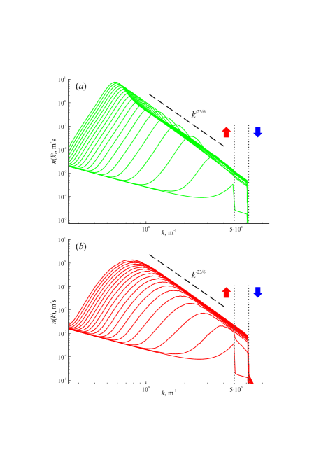
Figure 1: Development of wave action spectrum $n(k)$ under the action of constant wind $U=2c_{1}$, shown in steps of approximately $300\tau_{1}$, where $c_{1}$ and $\tau_{1}$ are characteristic phase speed and period, corresponding to $k=1$. (a) KE, WRT algorithm (b) DNS, with $\lambda_{k}=0.03$ on $161\times 71$ grid. Wavenumber ranges of forcing and dissipation are indicated by arrows

The neglect of weak non-gaussianity in the derivation of the KE makes its right-hand side a homogeneous function of $n(\mathbf{k})$ [8]. Basically, this means that the shape of the solutions for spectra provided by the KE corresponds to the case of infinitesimal amplitude. Thus the role of finite amplitude effects remains unknown. As the first attempt to study these effects, we compare numerical simulations based on the KE and the Zakharov equation (1). The Zakharov equation is simulated using the original algorithm, described in [20]. All parameters of the algorithm are the same as in [20], except for three modifications. First, in contrast to the simulations of swell in [20], we add wind forcing according to [24], for all $k<4.84$. Second, to accommodate the wider angular distribution of wind wave spectra, we increase the range of angles, retaining the same angular resolution. Thus, the computational grid contains 161 logarithmically spaced wavenumbers in the range $0.25\leq k\leq 9$ and 71 angles in the range $-7\pi/9\leq\theta\leq 7\pi/9$. Third, a DNS algorithm with wind forcing can only be functional if a certain parameterization of wave breaking is employed. Here we do not attempt to model the physical process of wave breaking, but intermittency in individual realisations makes it necessary to limit the growth of some wind amplified harmonics. To this end the following empirical rule is introduced: if non-dimensional value $\varepsilon_{k}=0.5\sqrt{2\omega n_{\mathbf{k}}/g}/\pi k$ exceeds $\varepsilon_{c}$, where $n_{\mathbf{k}}$ is the discrete wave action of a harmonic under forcing, then the forcing is changed to damping until $\varepsilon_{k}\leq 0.1\varepsilon_{c}$, when it is resumed. For the simulations with the $161\times 71$ grid, $\varepsilon_{c}$ is set to $0.01$, resulting in a small number of “breaking events”, usually between 0 and 5 for each realisation at every timestep. For the KE simulations, we use the standard WRT algorithm, provided by G. van Vledder, and $101\times 51$ grid with the same range of wavenumbers and full circle of directions. Wind forcing is identical for both models, dissipation is applied to $k\geq 6.25$.

Results.—First, we perform simulations of the wave field development from zero initial condition under forcing by constant wind with speed $U=2c_{1}$, where $c_{1}$ is the phase speed corresponding to $k=1$, close to the peak wavenumber at the end of the evolution. The DNS simulation is performed with averaging over 100 realizations. Development of the wave action spectrum $n(k)$ with time for both numerical methods is shown in figure 1. Comparison of the panels shows that both solutions tend to self-similar behaviour, and that the asymptotics of duration-limited wave growth under constant wave action flux, known from the analysis of the KE [9], are respected in both cases. However, the spectral shapes, which are initially close, differ considerably at later stages of the evolution. Although the spectral slope in both cases corresponds to the theoretical value for the inverse cascade of wave action $k^{-23/6}$ [21], the DNS spectra have less steep, more rounded spectral front and considerably wider and lower peak. Similar differences were reported earlier for simulations of wave evolution without wind forcing [20]. In the present case, the KE evolution also demonstrates a slightly faster downshift rate.

Due to the homogeneity property of the KE, the self-similar spectral shape is the same for all levels of nonlinearity, and the downshift rate has a simple scaling law [8]. If the discrepancies between the KE and the DNS are due to the effects of non-gaussianity unaccounted for by the KE, they are expected to decrease at lower levels of nonlinearity. Simulations with lower wind forcing indeed show that the difference in downshift rate decreases, but the difference in spectral shapes persists. Our aim to compare the DNS and the KE evolution in the small nonlinearity limit cannot be done by simply decreasing the wind speed, since wind-generated waves always have a certain finite steepness.

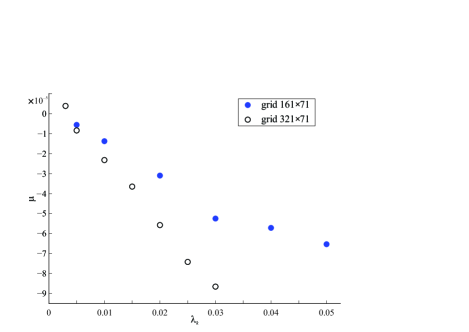
Figure 2: Non-gaussianity as measured by $\mu$, the ratio of statistically averaged nonlinear and linear energy as function of the coarse-graining parameter $\lambda_{k}$. $\mu$ is averaged over 600 characteristic periods of the final stage of evolution before the spectral peak reaches $k_{p}=1$.

Here we use another approach, which is helped by the particular design of the DNS algorithm. The algorithm is based on the idea of coarse-graining of a wave field [20], which relaxes the resonance condition into $\mathbf{k}_{0}+\mathbf{k}_{1}-\mathbf{k}_{2}-\mathbf{k}_{3}=\Delta\mathbf{k}$. In contrast to the standard condition $\Delta\mathbf{k}=0$, the wavevector and frequency mismatches satisfy $\Delta\omega/\omega_{min}<\lambda_{\omega}$, $|\Delta\mathbf{k}|/k_{min}<\lambda_{k}\bar{\omega}/\omega_{min}$, where $\omega_{\mathrm{min}}$ and $k_{\mathrm{min}}$ are the minimum values of frequency and wavenumber in the quartet, $\bar{\omega}$ is the mean frequency, and $\lambda_{\omega}$ and $\lambda_{k}$ are the detuning parameters. The crucial role is played by the coarse-graining parameter $\lambda_{k}$. If $\lambda_{k}=0$, the wave field in the canonically transformed space, in which both the Zakharov equation and the KE operate, is free (gaussian) regardless of the amplitude, since a logarithmically spaced grid with $\lambda_{k}=0$ allows no nontrivial wave interactions and, hence, no evolution. When $\lambda_{k}$ is increased, the number of approximately resonant interactions (with fixed $\lambda_{\omega}=0.01$) grows approximately quadratically with $\lambda_{k}$, while the rate of spectral evolution, measured by the rate of change of various integral parameters, quickly increases, until it reaches saturation at a certain value $\lambda_{k}$, dependent on grid resolution. Since in [20] the value $\lambda_{k}=0.03$ was found to be optimal for the $161\times 71$ grid, this value was used while computing the DNS evolution shown in figure 1. For the purpose of this study, it is convenient to use $\lambda_{k}$ as a way to create wave fields with the same level of nonlinearity $\varepsilon$, but different levels of non-gaussianity. In order to avoid discreteness effects at low number of interactions, we use the refined $321\times 71$ grid, along with the $161\times 71$ one, and $0.003\leq\lambda_{k}\leq 0.02$. Non-gaussianity can be measured as the ratio of the nonlinear part of the ensemble averaged Hamiltonian $\bar{H}$ [19]

$$\bar{H}_{NL}=\displaystyle\frac{1}{2}\int T_{0123}\langle b_{0}^{*}b_{1}^{*}b_{2}b_{3}\rangle\delta_{0+1-2-3}\,{\rm d}{\mathbf{k}}_{0123},$$ (5)

and its linear part $\bar{H}_{L}=\int\omega_{0}n_{0}\,{\rm d}{\mathbf{k}}_{0}$.

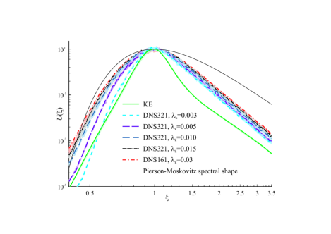
Figure 3: Self-similar shape function ${\cal U}(\xi)$, $\xi=kt^{6/11}$, extracted from the numerical solutions at the last 1000 wave periods of evolution. Shapes at every 100 periods are shown in light colours, the final curve is in darker colour of the same hue, normalized for ${\cal U}(1)=1$. Numerical models used are the KE and the DNS on $161\times 71$ (DNS161) and $321\times 71$ (DNS321) grids for different values of $\lambda_{k}$

Evolution of all wave fields is traced by the DNS with the same wind forcing as above, until the peak of wave action spectrum $n(k)$ reaches $k_{p}=1$. Under the wind forcing, linear and nonlinear parts of the Hamiltonian both grow with time, but their ratio $\mu=\bar{H}_{NL}/\bar{H}_{L}$ is approximately constant at the self-similar stage of evolution. The non-zero value of $\mu$, although very small, is a prerequisite for spectral evolution. Figure 2 shows the value of $\mu$ averaged over the last 600 periods of evolution before reaching $k_{p}=1$ for both grids, as function of $\lambda_{k}$. Non-gaussianity quickly grows with the increase of $\lambda_{k}$, approaching saturation at $\lambda_{k}\geq 0.03$. Meanwhile, the spectral evolution, as described by various integral parameters, does converge for both grids, and is very close between them. Formally, the value of $\lambda_{k}$ required for the simulation can be made smaller by further refinement of the grid, although in practice this is limited by the available computational resources. In particular, on the refined $321\times 71$ grid the number of wave interactions exceeds $10^{9}$ already for $\lambda_{k}=0.01$.

We are mainly interested in the shape of the spectrum. At the self-similar stage of evolution the spectral shape is characterized by the self-similar function $\cal U$ for the duration-limited evolution: $n(k)=at^{23/11}{\cal U}(bkt^{6/11})$, where $a$ and $b$ are constants [9]. The simulated self-similar spectral shapes ${\cal U}(\xi)$ are shown in figure 3. While the spectral slope depends on the parameterization of breaking more than on $\lambda_{k}$, the shape of the spectral front demonstrates a clear dependence on $\lambda_{k}$. For small $\lambda_{k}$, the wave field has relatively few wave interactions (about $10^{8}$ on the $321\times 71$ grid at $\lambda_{k}=0.003$), and the evolution is very slow, although the self-similar state is eventually reached, with the spectral front of the shape function ${\cal U}(\xi)$ close to the KE shape function. With the increase of $\lambda_{k}$ from zero, the shape function quickly approaches a different form, with a more rounded front and wider peak, resembling the Pierson-Moskowitz spectral shape.

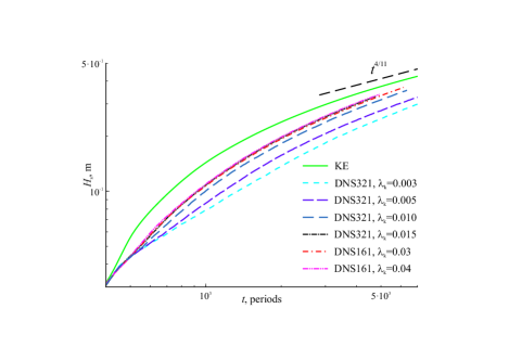
Figure 4: Evolution of significant wave height $H_{s}$: DNS on $161\times 71$ and $321\times 71$ grids for different values of $\lambda_{k}$ vs the KE simulation

For many applications, the evolution and prediction of integral charateristics of spectra, such as significant wave height, is of particular importance [4]. The important question is whether the evolution of integral characteristics can be affected by the effects of finite non-gaussianity for realistic wind speeds. To clarify this point, we plot in figure 4 the evolution of significant wave height $H_{s}$ obtained with the KE and the DNS for various values of $\lambda_{k}$. Figure 4 demonstrates that with the increase of $\lambda_{k}$ the DNS evolution of $H_{s}$ converges, remaining slightly slower than that predicted by the KE, but following the same asymptotic rate of increase known for the KE in the case of constant action flux [9]. The difference between the KE and the DNS is mostly manifested in the spectral shape, while the difference in significant wave height is relatively small and appears to be due to breaking that effectively reduces the forcing. Simulation of the KE with wind forcing reduced by 5% makes the difference insignificant.

Duscussion.—Studies of wave kinetics based on the KE rely on the homogeneity of the right-hand side of the equation with respect to the spectrum. This property is an artefact of the neglect of non-gaussianity effects. In this work, we show that although non-gaussianity is weak, in the long term it leads to considerable distortion of the spectral shape. At the same time, integral parameters of a wave field appear to be much less affected, with the error remaining within the uncertainty introduced by wave breaking, which the DNS modelling has to take into account. The spectral shape obtained by the DNS appears to be in much closer agreement with observations of mature sea states than the KE spectral shape.

The present study and its findings have numerous important implications. First, they are of crucial importance for all applications where the shape of the wave spectrum is significant, rather than just its integrated description, in particular for probability estimates of extreme wave events, design or coastal hazard risk assessments, sediment transport models, etc. Second, it is well known that the wind wave models based on the KE are optimized for certain frequency and directional resolutions against the available measurements. Knowledge of systematic errors in models can drastically improve the quality of such optimizations, and thus improve the quality of wind wave modelling. Third, the findings of this study provide an insight on the role of non-gaussianity in kinetic models, which is significant for a wide context of wave turbulence in various branches of physics.

Acknowledgments.—The work was supported by UK NERC grant NE/I01229X/1. Computations were performed on the CUDA High Performance Computing cluster at Keele University and on the ECMWF Supercomputing facility within the Special Project SPGBSHRI.

References

- Zakharov et al. [1992] V. Zakharov, V. L’vov, and G. Falkovich, Kolmogorov Spectra of Turbulence I: Wave Turbulence (Springer, 1992) p. 264.
- Newell and Rumpf [2013] A. Newell and B. Rumpf, in Advances in Wave Turbulence, A, Vol. 83, edited by V. Shrira and S. Nazarenko (World Scientific Series on Nonlinear Science, 2013) Chap. 1, pp. 1–51.
- Hasselmann [1962] K. Hasselmann, J. Fluid Mech. 12, 481 (1962).
- Komen et al. [1994] G. Komen, L. Cavaleri, M. Donelan, K. Hasselmann, S. Hasselmann, and P. A. E. M. Janssen, Dynamics and Modelling of Ocean Waves (Cambridge University Press, 1994) p. 532.
- Toba [1972] Y. Toba, J. Oceanogr. Soc. Japan 28, 109 (1972).
- Hasselmann et al. [1976] K. Hasselmann, D. Ross, P. Muller, and W. Sell, J. Phys. Oceanogr. 6, 200 (1976).
- Resio et al. [2016] D. Resio, L. Vincent, and D. Ardag, Ocean Modell. 103, 38 (2016).
- Zakharov et al. [2015] V. Zakharov, S. Badulin, P. Hwang, and G. Caulliez, J. Fluid Mech. 780, 503 (2015).
- Badulin et al. [2005] S. Badulin, A. Pushkarev, D. Resio, and V. Zakharov, Nonlin. Proc. Geophys. 12, 891 (2005).
- Holthuijsen [2007] L. Holthuijsen, Waves in Oceanic and Coastal Waters (Cambridge University Press, 2007) p. 404.
- Babanin and Soloviev [1998] A. Babanin and Y. Soloviev, J. Phys. Oceanogr. 28, 563 (1998).
- Long and Resio [2007] C. Long and D. Resio, J. Geophys. Res. 112, C05001 (2007).
- Romero and Melville [2010] L. Romero and W. Melville, J. Phys. Oceanogr. 40, 466 (2010).
- Pierson and Moskowitz [1964] W. Pierson and L. Moskowitz, J. Geophys. Res. 69, 5181 (1964).
- Alves et al. [2003] J. Alves, M. Banner, and I. Young, J. Phys. Oceanogr. 33, 1301 (2003).
- Banner et al. [2000] M. Banner, A. Babanin, and I. Young, J. Phys. Oceanogr. 30, 3145 (2000).
- Annenkov and Shrira [2006] S. Annenkov and V. Shrira, J. Fluid Mech. 561, 181 (2006).
- Annenkov and Shrira [2013] S. Annenkov and V. Shrira, J. Fluid Mech. 726, 517 (2013).
- Shrira and Annenkov [2013] V. Shrira and S. Annenkov, in Advances in Wave Turbulence, A, Vol. 83, edited by V. Shrira and S. Nazarenko (World Scientific Series on Nonlinear Science, 2013) Chap. 7, pp. 239–281.
- Annenkov and Shrira [2018] S. Annenkov and V. Shrira, J. Fluid Mech. 844, 766 (2018).
- Zakharov [1999] V. Zakharov, Eur. J. Mech. B/Fluids 18, 327 (1999).
- Onorato and Dematteis [2020] M. Onorato and G. Dematteis, J. Phys. Commun. 4, 095016 (2020).
- Newell et al. [2001] A. Newell, S. Nazarenko, and L. Biven, Physica D 152–153, 520 (2001).
- Hsiao and Shemdin [1983] S. Hsiao and O. Shemdin, J. Geophys. Res. 88, 9841 (1983).