Abstract

We study federated learning (FL)–especially cross-silo FL–with non-convex loss functions and data from people who do not trust the server or other silos. In this setting, each silo (e.g. hospital) must protect the privacy of each person’s data (e.g. patient’s medical record), even if the server or other silos act as adversarial eavesdroppers. To that end, we consider inter-silo record-level (ISRL) differential privacy (DP), which requires silo $i$’s communications to satisfy record/item-level DP. We propose novel ISRL-DP algorithms for FL with heterogeneous (non-i.i.d.) silo data and two classes of Lipschitz continuous loss functions: First, we consider losses satisfying the Proximal Polyak-Łojasiewicz (PL) inequality, which is an extension of the classical PL condition to the constrained setting. In contrast to our result, prior works only considered unconstrained private optimization with Lipschitz PL loss, which rules out most interesting PL losses such as strongly convex problems and linear/logistic regression. Our algorithms nearly attain the optimal strongly convex, homogeneous (i.i.d.) rate for ISRL-DP FL without assuming convexity or i.i.d. data. Second, we give the first private algorithms for non-convex non-smooth loss functions. Our utility bounds even improve on the state-of-the-art bounds for smooth losses. We complement our upper bounds with lower bounds. Additionally, we provide shuffle DP (SDP) algorithms that improve over the state-of-the-art central DP algorithms under more practical trust assumptions. Numerical experiments show that our algorithm has better accuracy than baselines for most privacy levels. All the codes are publicly available at: https://github.com/ghafeleb/Private-NonConvex-Federated-Learning-Without-a-Trusted-Server.

1 INTRODUCTION

Federated learning (FL) is a machine learning paradigm in which many “silos” (a.k.a. “clients”), such as hospitals, banks, or schools, collaborate to train a model by exchanging local updates, while storing their training data locally (Kairouz et al., 2019). Privacy has been an important motivation for FL due to decentralized data storage (McMahan et al., 2017). However, silo data can still be leaked in FL without additional safeguards (e.g. via membership or model inversion attacks) (Fredrikson et al., 2015; He et al., 2019; Song et al., 2020; Zhu and Han, 2020). Such leaks can occur when silos send updates to the central server—which an adversarial eavesdropper may access—or (in peer-to-peer FL) directly to other silos.

Differential privacy (DP) (Dwork et al., 2006) ensures that data cannot be leaked to an adversarial eavesdropper. Several variations of DP have been considered for FL. Numerous works (Jayaraman and Wang, 2018; Truex et al., 2019; Wang et al., 2019a; Kang et al., 2021; Noble et al., 2022) studied FL with central DP (CDP). Central DP provides protection for silos’ aggregated data against an adversary who only sees the final trained model. Central DP FL has two drawbacks: 1) the aggregate guarantee does not protect the privacy of each individual silo’s local data; and 2) it does not defend against privacy attacks from other silos or against an adversary with access to the server during training.

User-level DP (a.k.a. client-level DP) has been proposed as an alternative to central DP (McMahan et al., 2018; Geyer et al., 2017; Jayaraman and Wang, 2018; Gade and Vaidya, 2018; Wei et al., 2020a; Zhou and Tang, 2020; Levy et al., 2021; Ghazi et al., 2021a). User-level DP remedies the first drawback of CDP by preserving the privacy of every silo’s full local data set. Such a privacy guarantee is useful for cross-device FL, where each silo/client is associated with data from a single person (e.g. cell phone user) possessing many records (e.g. text messages). However, it is ill-suited for cross-silo FL, where silos (e.g. hospitals, banks, or schools) typically have data from many different people (e.g. patients, customers, or students). In cross-silo FL, each person’s (health, financial, or academic) record (or “item”) may contain sensitive information. Thus, it is desirable to ensure DP for each individual record (“item-level DP”) of silo $i$, instead of silo $i$’s full data set. Another crucial shortcoming of user-level DP is that, like central DP, it only guarantees the privacy of the final output of the FL algorithm against external adversaries: it does not protect against an adversary with access to the server, other silos, or the communications among silos during training.

While central DP and user-level DP implicitly assume that people (e.g. patients) trust all parties (e.g. their own hospital, other hospitals, and the server) with their private data, local DP (LDP) (Kasiviswanathan et al., 2011; Duchi et al., 2013) makes an extremely different assumption. In the LDP model, each person (e.g. patient) who contributes data does not trust anyone: not even their own silo (e.g. hospital) is considered trustworthy. In cross-silo FL, this assumption is unrealistic: e.g., patients typically want to share their accurate medical test results with their own doctor/hospital to get the best care possible. Therefore, LDP is often unnecessary and may be too stringent to learn useful/accurate models.

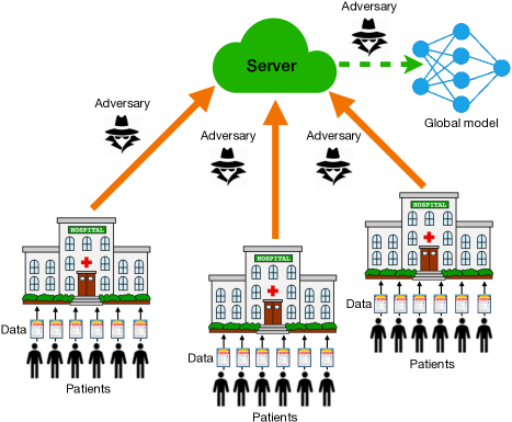
Figure 1: ISRL-DP ensures that each patient’s data cannot be leaked, even if the server/other silos collude to decode the data of hospital $i$. In contrast, user-level DP protects the full data of hospital $i$ and leaves hospitals vulnerable to attacks on the server.

In this work, we consider an intermediate privacy notion between the two extremes of local DP and central/user-level DP: inter-silo record-level differential privacy (ISRL-DP). ISRL-DP realistically assumes that people trust their own silo, but do not trust the server or other silos. An algorithm is ISRL-DP if all of the communications that silo $i$ sends satisfy item-level DP (for all $i$). See Figure 1 for a pictorial description and Section 1.1 for the precise definition. ISRL-DP eradicates all the drawbacks of central/user-level DP and local DP discussed above: 1) The item-level DP guarantee for each silo ensures that no person’s data (e.g. medical record) can be leaked. 2) Privacy of each silo’s communications protects silo data against attacks from an adversarial server and/or other silos. By post-processing (Dwork and Roth, 2014), it also implies that the final trained model is private. 3) By relaxing the overly strict trust assumptions of local DP, ISRL-DP allows for better model accuracy. ISRL-DP has been considered (under different names) in (Truex et al., 2020; Huang et al., 2020; Huang and Gong, 2020; Wu et al., 2019; Wei et al., 2020b; Dobbe et al., 2020; Zhao et al., 2020; Arachchige et al., 2019; Seif et al., 2020; Lowy and Razaviyayn, 2021b; Noble et al., 2022; Liu et al., 2022b).

Although ISRL-DP was largely motivated by cross-silo applications, it can also be useful in cross-device FL without a trusted server. This is because ISRL-DP implies user-level DP if the ISRL-DP parameter is small enough: see Appendix B and also (Lowy and Razaviyayn, 2021b). However, unlike user-level DP, ISRL-DP has the benefit of preventing leaks to the untrusted server and other users.

Another intermediate DP notion between the low-trust local models and the high-trust central/user-level models is the shuffle model of DP (Bittau et al., 2017; Cheu et al., 2019; Erlingsson et al., 2020a, b; Feldman et al., 2020; Liu et al., 2020; Girgis et al., 2021; Ghazi et al., 2021b). In the shuffle model, silos send their local updates to a secure shuffler. The shuffler randomly permutes silos’ updates (anonymizing them), and then sends the shuffled messages to the server. $\mathcal{A}$ is shuffle DP (SDP) if the shuffled messages satisfy central DP. Figure 2 compares the trust assumptions of the different notions of DP FL discussed above.

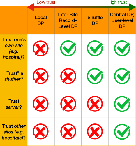
Figure 2: Trust assumptions of DP FL notions. “Trust” is in quotes because silo messages must already satisfy (at least a weak level of) ISRL-DP in order to realize SDP: anonymization alone cannot provide DP (Dwork and Roth, 2014).

Problem setup: Consider a horizontal FL setting with $N$ silos (e.g. hospitals). Each silo has a local data set with $n$ samples (e.g. patient records): $X_{i}=(x_{i,1},\cdots,x_{i,n})\in\mathcal{X}^{n}$ for $i\in[N]\triangleq\{1,\cdots,N\}$. Let $X_{i}\sim\mathcal{D}_{i}^{n}$, for unknown distributions $\mathcal{D}_{i}$, which may vary across silos (“heterogeneous”). In the $r$-th round of communication, silos receive the global model $w_{r}$ from the server and use their local data to improve the model. Then, silos send local updates to the server (or other silos, in peer-to-peer FL), who updates the global model to $w_{r+1}$. Given a loss function $f:\mathbb{R}^{d}\times\mathcal{X}\to\mathbb{R}\bigcup\{+\infty\}$, let

$$F_{i}(w):=\mathbb{E}_{x_{i}\sim\mathcal{D}_{i}}[f(w,x_{i})].\vspace{-0.12cm}$$ (1)

At times, we consider empirical risk minimization (ERM), with $\widehat{F}_{i}(w):=\frac{1}{n}\sum_{j=1}^{n}f(w,x_{i,j})$. We aim to solve the FL problem:

$$\min_{w\in\mathbb{R}^{d}}\left\{F(w):=\frac{1}{N}\sum_{i=1}^{N}F_{i}(w)\right\},$$ (2)

or $\min_{w\in\mathbb{R}^{d}}\{\widehat{F}_{\mathbf{X}}(w):=\frac{1}{N}\sum_{i=1}^{N}\widehat{F}_{i}(w)\}\normalsize$ for ERM, while keeping silo data private. Here $\mathbf{X}=(X_{1},\cdots,X_{N})\in\mathcal{X}_{1}^{n}\times\cdots\times\mathcal{X}_{N}^{n}=:\mathbb{X}$ is a distributed database. We allow for constrained FL by considering $f$ that takes the value $+\infty$ outside of some closed set $\mathcal{W}\subset\mathbb{R}^{d}$. When $F_{i}$ takes the form 1 (not necessarily ERM), we refer to the problem as stochastic optimization (SO) for emphasis. For SO, we assume that the samples $x_{i,j}$ are independent. For ERM, we make no assumptions on the data. The excess risk of an algorithm $\mathcal{A}$ for solving 2 is $\mathbb{E}F(\mathcal{A}(\mathbf{X}))-F^{*}$, where $F^{*}=\inf_{w}F(w)$ and the expectation is taken over both the random draw of $\mathbf{X}=(X_{1},\ldots,X_{N})$ and the randomness of $\mathcal{A}$. For ERM, the excess empirical risk of $\mathcal{A}$ is $\mathbb{E}\widehat{F}_{\mathbf{X}}(\mathcal{A}(\mathbf{X}))-\widehat{F}_{\mathbf{X}}^{*}$, where the expectation is taken solely over the randomness of $\mathcal{A}$. For general non-convex loss functions, meaningful excess risk guarantees are not tractable in polynomial time. Thus, we use the norm of the gradient to measure the utility (stationarity) of FL algorithms.

Contributions and Related Work: For (strongly) convex losses, the optimal performance of ISRL-DP and SDP FL algorithms is mostly understood (Lowy and Razaviyayn, 2021b; Girgis et al., 2021). In this work, we consider the following questions for non-convex losses:

Question 1. What is the best performance that any inter-silo record-level DP algorithm can achieve for solving 2 with non-convex $F$? Question 2. With a trusted shuffler (but no trusted server), what performance is attainable?

Our first contribution in Section 2.1 is a nearly complete answer to Questions 1 and 2 for the subclass of non-convex loss functions that satisfy the Proximal Polyak-Łojasiewicz (PL) inequality (Karimi et al., 2016). The Proximal PL (PPL) condition is a generalization of the classical PL inequality (Polyak, 1963) and covers many important ML models: e.g. some classes of neural nets such as wide neural nets (Liu et al., 2022a; Lei and Ying, 2021), linear/logistic regression, LASSO, strongly convex losses (Karimi et al., 2016). For heterogeneous FL with non-convex proximal PL losses, our ISRL-DP algorithm attains excess risk that nearly matches the strongly convex, i.i.d. lower bound (Lowy and Razaviyayn, 2021b). Additionally, the excess risk of our SDP algorithm nearly matches the strongly convex, i.i.d., central DP lower bound (Bassily et al., 2019) and is attained without convexity, without i.i.d. data, and without a trusted server. Our excess risk bounds nearly match the optimal statistical rates in certain practical parameter regimes, resulting in “privacy almost for free.”

To obtain these results, we invent a new method of analyzing noisy proximal gradient algorithms that does not require convexity, applying tools from the analysis of objective perturbation (Chaudhuri et al., 2011; Kifer et al., 2012). Our novel analysis is necessary because privacy noise cannot be easily separated from the non-private optimization terms in the presence of the proximal operator and non-convexity.

Our second contribution in Section 2.2 is a nearly complete answer to Questions 1 and 2 for federated ERM with proximal PL losses. We provide novel, communication-efficient, proximal variance-reduced ISRL-DP and SDP algorithms for non-convex ERM. Our algorithms have near-optimal excess empirical risk that almost match the strongly convex ISRL-DP and CDP lower bounds (Lowy and Razaviyayn, 2021b; Bassily et al., 2014), without requiring convexity.

Prior works (Wang et al., 2017; Kang et al., 2021; Zhang et al., 2021) on DP PL optimization considered an extremely narrow PL function class: unconstrained optimization with Lipschitz continuous losses satisfying the classical PL inequality (Polyak, 1963). The combined assumptions of Lipschitz continuity and the PL condition on $\mathbb{R}^{d}$ (unconstrained) are very strong and rule out most interesting PL losses (e.g. neural nets, linear/logistic regression, LASSO, strongly convex), since the Lipschitz parameter of such losses is infinite or prohibitively large. By contrast, the Proximal PL function class that we consider allows for such losses, which are Lipschitz on a restricted parameter domain.

Third, we address Questions 1 and 2 for general non-convex/non-smooth (non-PL) loss functions in Section 3. We develop the first DP optimization (in particular, FL) algorithms for non-convex/non-smooth loss functions. Our ISRL-DP and SDP algorithms have significantly better utility than all previous ISRL-DP and CDP FL algorithms for smooth losses (Wang et al., 2019a; Ding et al., 2021; Hu et al., 2021; Noble et al., 2022). We complement our upper bound with the first non-trivial ISRL-DP lower bound for non-convex FL in Section 3.1.

As a consequence of our analyses, we also obtain bounds for FL algorithms that satisfy both ISRL-DP and user-level DP simultaneously, in  Appendix G. Such a privacy requirement would be useful in cross-device FL with users (e.g. cell phone) who do not trust the server or other users with their sensitive data (e.g. text messages).

Finally, numerical experiments in Section 4 showcase the practical performance of our algorithm on several benchmark data sets. In each experiment, our algorithm attains better accuracy than the baselines for most privacy levels.

See Fig. 3 for a summary of our results and Appendix C for a thorough discussion of related work.

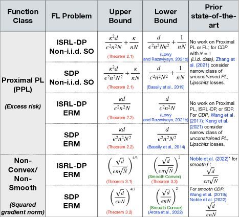
Figure 3: Summary of results for $M=N$, log terms omitted. $\kappa=\beta/\mu$, where $\beta$ is the smoothness parameter and $\mu$ is the proximal-PL parameter of the loss. *(Noble et al., 2022) mostly analyzes CDP FL but we observe that a ISRL-DP bound can also be obtained with a small modification of their algorithm and analysis.

1.1 Preliminaries

Differential Privacy: Let $\mathbb{X}=\mathcal{X}_{1}^{n}\times\cdots\mathcal{X}^{n}$ and $\rho:\mathbb{X}^{2}\to[0,\infty)$ be a distance between databases. Two databases $\mathbf{X},\mathbf{X}^{\prime}\in\mathbb{X}$ are $\rho$-adjacent if $\rho(\mathbf{X},\mathbf{X}^{\prime})\leq 1$. DP ensures that (with high probability) an adversary cannot distinguish between the outputs of algorithm $\mathcal{A}$ when it is run on adjacent databases:

Definition 1 (Differential Privacy).

Let $\epsilon\geq 0,~{}\delta\in[0,1).$ A randomized algorithm $\mathcal{A}:\mathbb{X}\to\mathcal{W}$ is $(\epsilon,\delta)$-differentially private (DP) (with respect to $\rho$) if for all $\rho$-adjacent data sets $\mathbf{X},\mathbf{X}^{\prime}\in\mathbb{X}$ and all measurable subsets $S\subseteq\mathcal{W}$, we have

$$\mathbb{P}(\mathcal{A}(\mathbf{X})\in S)\leq e^{\epsilon}\mathbb{P}(\mathcal{A}(\mathbf{X}^{\prime})\in S)+\delta.$$ (3)

Definition 2 (Inter-Silo Record-Level Differential Privacy).

Let $\rho_{i}:\mathcal{X}^{2}\to[0,\infty)$, $\rho_{i}(X_{i},X^{\prime}_{i}):=\sum_{j=1}^{n}\mathds{1}_{\{x_{i,j}\neq x_{i,j}^{\prime}\}}$, $i\in[N]$. A randomized algorithm $\mathcal{A}$ is $(\epsilon,\delta)$-ISRL-DP if for all $i\in[N]$ and all $\rho_{i}$-adjacent silo data sets $X_{i},X^{\prime}_{i}$, the full transcript of silo $i$’s sent messages satisfies 3 for any fixed settings of other silos’ messages and data.

Definition 3 (Shuffle Differential Privacy (Bittau et al., 2017; Cheu et al., 2019)).

A randomized algorithm $\mathcal{A}$ is $(\epsilon,\delta)$-shuffle DP (SDP) if for all $\rho$-adjacent databases $\mathbf{X},\mathbf{X}^{\prime}\in\mathbb{X}$ and all measurable subsets $S$, the collection of all uniformly randomly permuted messages that are sent by the shuffler satisfies 3, with $\rho(\mathbf{X},\mathbf{X}^{\prime}):=\sum_{i=1}^{N}\sum_{j=1}^{n}\mathds{1}_{\{x_{i,j}\neq x^{\prime}_{i,j}\}}$.

In Appendix D, we recall the basic DP building blocks that our algorithms employ.

Notation and Assumptions: Denote by $\|\cdot\|$ the $\ell_{2}$ norm. Let $\mathcal{W}$ be a closed convex set. For differentiable (w.r.t. $w$) $f^{0}:\mathcal{W}\times\mathcal{X}\to\mathbb{R}$, denote its gradient w.r.t. $w$ by $\nabla f^{0}(w,x)$. Function $h$ is $\beta$-smooth if $\nabla h$ is $\beta$-Lipschitz. A proper function has range $\mathbb{R}\bigcup\{+\infty\}$ and is not identically equal to $+\infty$. Function $g$ is closed if $\forall\alpha\in\mathbb{R}$, the set $\{w\in\mbox{dom}(g)|g(w)\leq\alpha\}$ is closed. The indicator function of $\mathcal{W}$ is $\iota_{\mathcal{W}}(w):=\begin{cases}0&\mbox{if $w\in\mathcal{W}$}\\ +\infty&\mbox{otherwise}\end{cases}.$ The proximal operator of function $f^{1}$ is $\texttt{{prox}}_{\eta f^{1}}(z):=\operatorname*{argmin}_{y\in\mathbb{R}^{d}}\left(\eta f^{1}(y)+\frac{1}{2}\|y-z\|^{2}\right),~{}\text{for}~{}\eta>0.$ Write $a\lesssim b$ if $\exists C>0$ such that $a\leq Cb$ and $a=\widetilde{\mathcal{O}}(b)$ if $a\lesssim\log^{2}(\theta)b$ for some parameters $\theta$. Let $\hat{\Delta}_{\mathbf{X}}:=\widehat{F}_{\mathbf{X}}(w_{0})-\widehat{F}_{\mathbf{X}}^{*}$, with $\widehat{F}_{\mathbf{X}}^{*}=\inf_{w}\widehat{F}_{\mathbf{X}}(w)$. We assume the loss function $f(w,x)=f^{0}(w,x)+f^{1}(w)$ is non-convex/non-smooth composite, where $f^{0}$ is bounded below, and:

Assumption 1.

$f^{0}(\cdot,x)$ is $L$-Lipschitz (on $\mathcal{W}$ if $f^{1}=\iota_{\mathcal{W}}+g$ for some convex $g\geq 0$; on $\mathbb{R}^{d}$ otherwise) and $\beta$-smooth for all $x\in\mathcal{X}$.

Assumption 2.

$f^{1}$ is a proper, closed, convex function.

Examples of functions satisfying Assumption 2 include indicator functions of convex sets $\iota_{\mathcal{W}}$ and $\ell_{p}$-regularizers $\lambda\|w\|_{p}$ with $p\in[1,\infty]$. We allow FL networks in which some silos may be unable to participate in every round (e.g. due to internet/wireless communication problems):

Assumption 3.

In each round of communication $r$, a uniformly random subset $S_{r}$ of $M=|S_{r}|\in[N]$ silos receives the global model and can send messages.

Assumption 3 is realistic for cross-device FL. However, in cross-silo FL, typically $M\approx N$ (Kairouz et al., 2019).

2 ALGORITHMS FOR PROXIMAL-PL LOSSES

2.1 Noisy Distributed Proximal SGD for Heterogeneous FL (SO)

We propose a simple distributed Noisy Proximal SGD (Prox-SGD) method: in each round $r\in[R]$, available silos $i\in S_{r}$ draw local samples $\{x_{i,j}^{r}\}_{j=1}^{K:=\lfloor n/R\rfloor}$ from $X_{i}$ (without replacement) and compute $\widetilde{g}_{r}^{i}:=\frac{1}{K}\sum_{j=1}^{K}\nabla f^{0}(w_{r},x_{i,j}^{r})+u_{i}$, where $u_{i}\sim\mathcal{N}(0,\sigma^{2}\mathbf{I}_{d})$ for ISRL-DP. For SDP, $u_{i}$ has Binomial distribution (Cheu et al., 2021). The server (or silos) aggregates $\widetilde{g}_{r}:=\frac{1}{M}\sum_{i\in S_{r}}\widetilde{g}_{r}^{i}$ and then updates the global model $w_{r+1}:=\texttt{{prox}}_{\frac{1}{2\beta}f^{1}}(w_{r}-\frac{1}{2\beta}\widetilde{g}_{r})$. The use of prox is needed to handle the potential non-smoothness of $f$. Pseudocodes are in Section E.1.

Assumption 4.

The loss is $\mu$-PPL in expectation: $\forall w\in\mathbb{R}^{d}$,

$$\mu\mathbb{E}[\widehat{F}_{\cal{S}}(w)-\inf_{w^{\prime}}\widehat{F}_{\cal{S}}(w^{\prime})] \leq-\beta\mathbb{E}\Bigg{[}\min_{y}\Big{[}\langle\nabla\widehat{F}_{\cal{S}}^{0}(w),y-w\rangle$$

$$\;\;+\frac{\beta}{2}\|y-w\|^{2}+f^{1}(y)-f^{1}(w)\Big{]}\Bigg{]},\vspace{-.02in}$$

where $\widehat{F}_{\cal{S}}(w):=\frac{1}{MK}\sum_{i\in S}\sum_{j=1}^{K}f(w,x_{i,j})$, $S\subseteq[N]$ is a uniformly random subset of size $M$, $\mathcal{S}=\{x_{i,j}\}_{i\in S,j\in[K]}$, and $x_{i,j}\sim\mathcal{D}_{i}$. Denote $\kappa=\beta/\mu$.

As discussed earlier, many interesting losses (e.g. neural nets, linear regression) satisfy Assumption 4.

Theorem 2.1 (Noisy Prox-SGD: Heterogeneous PPL FL).

Grant Assumption 4. Let $\epsilon\leq\min\{8\ln(1/\delta),15\},\delta\in(0,1/2)$, $n\geq\widetilde{\Omega}(\kappa)$. Then, there exist $\sigma^{2}$ and $K$ such that:
1. ISRL-DP Prox-SGD is $(\epsilon,\delta)$-ISRL-DP, and in $R=\widetilde{\mathcal{O}}(\kappa)$ communications, we have:

$$\mathbb{E}F(w_{R})-F^{*}=\widetilde{\mathcal{O}}\left(\frac{L^{2}}{\mu}\left(\frac{\kappa^{2}d\ln(1/\delta)}{\epsilon^{2}n^{2}M}+\frac{\kappa}{Mn}\right)\right).$$ (4)

2. SDP Prox-SGD is $(\epsilon,\delta)$-SDP for $M\geq N\min(\epsilon/2,1)$, and if $R=\widetilde{\mathcal{O}}(\kappa)$, then:

$$\mathbb{E}F(w_{R})-F^{*}=\widetilde{\mathcal{O}}\left(\frac{L^{2}}{\mu}\left(\frac{\kappa^{2}d\ln^{2}(d/\delta)}{\epsilon^{2}n^{2}N^{2}}+\frac{\kappa}{Mn}\right)\right).$$ (5)

Remark 2.1 (Near-Optimality and “privacy almost for free”).

Let $M=N$. Then, the bound in 5 nearly matches the central DP strongly convex, i.i.d. lower bound of (Bassily et al., 2019) up to the factor $\widetilde{O}(\kappa^{2})$ without a trusted server, without convexity, and without i.i.d. silos. Further, if $\kappa d\log^{2}(d/\delta)/\epsilon^{2}\lesssim nN$, then 5 matches the non-private strongly convex, i.i.d. lower bound of (Agarwal et al., 2012) up to a $\widetilde{\mathcal{O}}(\kappa)$ factor, providing privacy nearly for free, without convexity/homogeneity. The bound in 4 is larger than the i.i.d., strongly convex, ISRL-DP lower bound of (Lowy and Razaviyayn, 2021b) by a factor of $\widetilde{\mathcal{O}}(\kappa^{4})$. Moreover, if $\kappa d\ln(1/\delta)/\epsilon^{2}\lesssim n$, then the ISRL-DP rate in 4 matches the non-private, strongly convex, i.i.d. lower bound (Agarwal et al., 2012) up to $\widetilde{\mathcal{O}}(\kappa)$.

Theorem 2.1 is proved in Section E.2. Privacy follows from parallel composition (McSherry, 2009) and the guarantees of the Gaussian mechanism (Dwork and Roth, 2014) and binomial-noised shuffle vector summation protocol (Cheu et al., 2021). The main idea of the excess loss proofs is to view each noisy proximal evaluation as an execution of objective perturbation (Chaudhuri et al., 2011). Using techniques from the analysis of objective perturbation, we bound the key term arising from descent lemma by the corresponding noiseless minimum plus an error term that scales with $\|\frac{1}{M}\sum_{i\in S_{r}}u_{i}\|^{2}$.

Our novel proof approach is necessary because with the proximal operator and without convexity, privacy noise cannot be easily separated from the non-private terms. By comparison, in the convex case, the proof of (Lowy and Razaviyayn, 2021b, Theorem 2.1) uses non-expansiveness of projection and independence of the noise and data to bound $\mathbb{E}\|w_{r+1}-w_{r}\|^{2}$, which yields a bound on $\mathbb{E}F(w_{r})-F^{*}$ by convexity. On the other hand, in the unconstrained PL case considered in (Wang et al., 2017; Kang et al., 2021; Zhang et al., 2021), the excess loss proof is easy, but the result is essentially vacuous since Lipschitzness on $\mathbb{R}^{d}$ is incompatible with all PL losses that we are aware of. The works mentioned above considered the simpler i.i.d. or ERM cases: Balancing divergent silo distributions and privately reaching consensus on a single parameter $w_{R}$ that optimizes the global objective $F$ poses an additional difficulty.

2.2 Noisy Distributed Prox-PL-SVRG for Federated ERM

In this subsection, we assume $\widehat{F}_{\mathbf{X}}$ satisfies the proximal-PL inequality with parameter $\mu>0$; i.e. for all $w\in\mathbb{R}^{d}$:

$$\mu[\widehat{F}_{\mathbf{X}}(w)-\inf_{w^{\prime}}\widehat{F}_{\mathbf{X}}(w^{\prime})] \leq-\beta\min_{y}\Big{[}\langle\nabla\widehat{F}_{\mathbf{X}}^{0}(w),y-w\rangle$$

$$\;\;\;+\frac{\beta}{2}\|y-w\|^{2}+\widehat{F}_{\mathbf{X}}^{1}(y)-\widehat{F}_{\mathbf{X}}^{1}(w)\Big{]}.$$

We propose new, variance-reduced accelerated ISRL-DP/SDP algorithms in order to achieve near-optimal rates in fewer communication rounds than would be possible with Noisy Prox-SGD. Our ISRL-DP Algorithm 2 for Proximal PL ERM, which builds on (J Reddi et al., 2016), iteratively runs ISRL-DP Prox-SVRG (Algorithm 1) with re-starts. See Section E.3 for our SDP algorithm, which is nearly identical to Algorithm 2 except that we use the binomial noise-based shuffle protocol of (Cheu et al., 2021) instead of Gaussian noise.

Algorithm 1 ISRL-DP FedProx-SVRG $(w_{0})$

1:  Input: $E\in\mathbb{N},K\in[n],Q:=\lfloor\frac{n}{K}\rfloor,\mathbf{X}\in\mathbb{X},\eta>0,\sigma_{1},\sigma_{2}\geq 0,\widebar{w}_{0}=w_{0}^{Q}=w_{0}\in\mathbb{R}^{d}$.

2:  for $r\in\{0,1,\cdots,E-1\}$ do

3:     Server updates $w^{0}_{r+1}=w^{Q}_{r}$.

4:     for $i\in S_{r}$ in parallel do

5:        Server sends global model $w_{r}$ to silo $i$.

6:        Silo $i$ draws noise $u^{i}_{1}\sim\mathcal{N}(0,\sigma_{1}^{2}\mathbf{I}_{d})$ and computes $\widetilde{g}_{r+1}^{i}:=\nabla\widehat{F}_{i}^{0}(\widebar{w}_{r})+u^{i}_{1}$.

7:        for $t\in\{0,1,\cdots Q-1\}$ do

8:           Silo $i$ draws $K$ samples $x_{i,j}^{r+1,t}$ uniformly from $X_{i}$ with replacement (for $j\in[K]$) and noise $u^{i}_{2}\sim\mathcal{N}(0,\sigma_{2}^{2}\mathbf{I}_{d})$.

9:           Silo $i$ computes $\widetilde{v}_{r+1}^{t,i}=\frac{1}{K}\sum_{j=1}^{K}[\nabla f^{0}(w_{r+1}^{t},x_{i,j}^{r+1,t})-\nabla f^{0}(\widebar{w}_{r},x_{i,j}^{r+1,t})]+\widetilde{g}_{r+1}^{i}+u_{2}^{i}$.

10:           Server aggregates $\widetilde{v}_{r+1}^{t}=\frac{1}{M}\sum_{i\in S_{r+1}}\widetilde{v}_{r+1}^{t,i}$, updates $w_{r+1}^{t+1}:=\texttt{{prox}}_{\eta f^{1}}(w_{r+1}^{t}-\eta\widetilde{v}_{r+1}^{t})$.

11:        end for

12:        Server updates $\widebar{w}_{r+1}=w_{r+1}^{Q}$.

13:     end for

14:  end for

15:  Output: $w_{\text{priv}}\sim\text{Unif}(\{w_{r+1}^{t}\}_{r=0,\cdots,E-1;t=0,\cdots Q-1})$.

Algorithm 2 ISRL-DP FedProx-PL-SVRG

1:  Input: $E\in\mathbb{N},K\in[n],Q:=\lfloor\frac{n}{K}\rfloor,\mathbf{X}\in\mathbb{X},\eta>0,\sigma_{1},\sigma_{2}\geq 0,\widebar{w}_{0}=w_{0}^{Q}=w_{0}\in\mathbb{R}^{d}$.

2:  for $s\in[S]$ do

3:     $w_{s}=\texttt{ISRL-DP FedProx-SVRG}(w_{s-1})$

4:  end for

5:  Output: $w_{\text{priv}}:=w_{S}$.

The key component of ISRL-DP Prox-SVRG is in line 9 of Algorithm 1, where instead of using standard noisy stochastic gradients, silo $i$ computes the difference between the stochastic gradient at the current iterate $w_{r+1}^{t}$ and the iterate $\widebar{w}_{r}$ from the previous epoch, thereby reducing the variance of the noisy gradient estimator–which is still unbiased–and facilitating faster convergence (i.e. better communication complexity). Notice that the $\ell_{2}$-sensitivity of the variance-reduced gradient in line 9 is larger than the sensitivity of standard stochastic gradients (e.g. in line 6), so larger $\sigma_{2}^{2}>\sigma_{1}^{2}$ is required for ISRL-DP. However, the sensitivity only increases by a constant factor, which does not significantly affect utility. Algorithm 2 runs Algorithm 1 $S$ times with re-starts. For a suitable choice of algorithmic parameters, we have:

Theorem 2.2 (Noisy Prox-PL-SVRG: ERM).

Let $\epsilon\leq\min\{15,2\ln(2/\delta)\},\delta\in(0,1/2)$, $M=N$, $\mathbf{X}\in\mathcal{X}^{n}$, and $\kappa=\beta/\mu$. Then, in $\widetilde{\mathcal{O}}(\kappa)$ communication rounds, we have:
1. ISRL-DP Prox-PL-SVRG is $(\epsilon,\delta)$-ISRL-DP and  $\mathbb{E}\widehat{F}_{\mathbf{X}\normalsize}(w_{\text{priv}})-\widehat{F}_{\mathbf{X}\normalsize}^{*}=\widetilde{\mathcal{O}}\left(\kappa\frac{L^{2}d\ln(1/\delta)}{\mu\epsilon^{2}n^{2}N}\right).$
2. SDP Prox-PL-SVRG is $(\epsilon,\delta)$-SDP and  $\mathbb{E}\widehat{F}_{\mathbf{X}\normalsize}(w_{\text{priv}})-\widehat{F}_{\mathbf{X}\normalsize}^{*}=\widetilde{\mathcal{O}}\left(\kappa\frac{L^{2}d\ln(1/\delta)}{\mu\epsilon^{2}n^{2}N^{2}}\right).$

Expectations are solely over $\mathcal{A}$. A similar result holds for $M<N$, provided silo data is not too heterogeneous. See Section E.4 for details and the proof.

Remark 2.2 (Near-Optimality).

The ISRL-DP and SDP bounds in Theorem 2.2 nearly match (respectively) the ISRL-DP and CDP strongly convex ERM lower bounds (Lowy and Razaviyayn, 2021b; Bassily et al., 2014) (for $f^{1}=\iota_{\mathcal{W}})$) up to the factor $\widetilde{\mathcal{O}}(\kappa)$, and are attained without convexity.

3 ALGORITHMS FOR NON-CONVEX/NON-SMOOTH COMPOSITE LOSSES

In this section, we consider private FL with general non-convex/non-smooth composite losses: i.e. we make no additional assumptions on $f$ beyond Assumption 1 and Assumption 2. In particular, we do not assume the Proximal PL condition, allowing for a range of constrained/unconstrained non-convex and non-smooth FL problems. For such a function class, finding global optima is not possible in polynomial time; optimization algorithms may only find stationary points in polynomial time. Thus, we measure the utility of our algorithms in terms of the norm of the proximal gradient mapping:

$$\widehat{\mathcal{G}}_{\eta}(w,\mathbf{X}):=\frac{1}{\eta}[w-\texttt{{prox}}_{\eta f^{1}}(w-\eta\nabla\widehat{F}_{\mathbf{X}}^{0}(w))]$$

For proximal algorithms, this is a natural measure of stationarity (J Reddi et al., 2016; Wang et al., 2019b) which generalizes the standard (for smooth unconstrained) notion of first-order stationarity. In the smooth unconstrained case, $\|\widehat{\mathcal{G}}_{\eta}(w,\mathbf{X})\|$ reduces to $\|\nabla\widehat{F}_{\mathbf{X}}(w)\|$, which is often used to measure convergence in non-convex optimization. Building on (Fang et al., 2018; Wang et al., 2019b; Arora et al., 2022), we propose Algorithm 3 for ISRL-DP FL with non-convex/non-smooth composite losses. Algorithm 3 is inspired by the optimality of non-private SPIDER for non-convex ERM (Arjevani et al., 2019).

Algorithm 3 ISRL-DP FedProx-SPIDER

1:  Input: $R\in\mathbb{N},K_{1},K_{2}\in[n],\mathbf{X}\in\mathbb{X},\eta>0,\sigma_{1}^{2},\sigma_{2}^{2},\hat{\sigma}_{2}^{2}\geq 0,q\in\mathbb{N},w_{0}\in\mathcal{W}$.

2:  for $r\in\{0,1,\cdots,R\}$ do

3:     for $i\in S_{r}$ in parallel do

4:        Server sends global model $w_{r}$ to silo $i$.

5:        if $r\equiv 0~{}(\text{mod}~{}q)$ then

6:           Silo $i$ draws $K_{1}$ samples $\{x_{i,j}^{r}\}_{j=1}^{K_{1}}$ u.a.r. from $X_{i}$ (with replacement) and $u_{1}^{i}\sim\mathcal{N}(0,\sigma_{1}^{2}\mathbf{I}_{d})$.

7:           Silo $i$ computes $h_{r}^{i}=\frac{1}{K_{1}}\sum_{j=1}^{K_{1}}\nabla f^{0}(w_{r},x_{i,j}^{r})+u_{1}^{i}$.

8:           Server aggregates $h_{r}=\frac{1}{M_{r}}\sum_{i\in S_{r}}h_{r}^{i}$.

9:        else

10:           Silo $i$ draws $K_{2}$ samples $\{x_{i,j}^{r}\}_{j=1}^{K_{1}}$ u.a.r. from $X_{i}$ (with replacement) and $u_{2}^{i}\sim\mathcal{N}(0,\mathbf{I}_{d}\min\{\sigma_{2}^{2}\|w_{r}-w_{r-1}\|^{2},\hat{\sigma}_{2}^{2}\})$.

11:           Silo $i$ computes $H_{r}^{i}=\frac{1}{K_{2}}\sum_{j=1}^{K_{2}}[\nabla f^{0}(w_{r},x_{i,j}^{r})-\nabla f^{0}(w_{r-1},x_{i,j}^{r})]+u_{2}^{i}$.

12:           Server aggregates $H_{r}=\frac{1}{M_{r}}\sum_{i\in S_{r}}H_{r}^{i}$ and $h_{r}=h_{r-1}+H_{r}$.

13:        end if

14:     end for

15:     Server updates $w_{r+1}=\texttt{{prox}}_{\eta f^{1}}(w_{r}-\eta h_{r})$.

16:  end for

17:  Output: $w_{\text{priv}}\sim\text{Unif}(\{w_{r}\}_{r=1,\cdots,R})$.

The essential elements of the algorithms are: the variance-reduced Stochastic Path-Integrated Differential EstimatoR of the gradient in line 11; and the non-standard choice of privacy noise in line 10 (inspired by (Arora et al., 2022)), in which we choose $\sigma_{2}^{2}=\frac{16\beta^{2}R\ln(1/\delta)}{\epsilon^{2}n^{2}}$. With careful choices of $\eta,\sigma_{1}^{2},\hat{\sigma}_{2}^{2},q,R$ in ISRL-DP FedProx-SPIDER, our algorithm achieves state-of-the-art utility:

Theorem 3.1 (ISRL-DP FedProx-SPIDER, $M=N$ version).

Let $\epsilon\leq 2\ln(1/\delta)$. Then, ISRL-DP FedProx-SPIDER is $(\epsilon,\delta)$-ISRL-DP. Moreover, if $M=N$, then

$$\mathbb{E}\|\widehat{\mathcal{G}}_{\eta}(w_{\text{priv}},\mathbf{X})\|^{2}\lesssim\left(\frac{\sqrt{L\beta\hat{\Delta}_{\mathbf{X}}d\ln(1/\delta)}}{\epsilon n\sqrt{N}}\right)^{4/3}+\frac{L^{2}d\ln(1/\delta)}{\epsilon^{2}n^{2}N}.\normalsize\vspace{-.2cm}$$

See Appendix F for the general statement for $M\leq N$, and the detailed proof. Theorem 3.1 provides the first utility bound for any kind of DP optimization problem (even centralized) with non-convex/non-smooth losses. In fact, the only work we are aware of that addresses DP non-convex optimization with $f^{1}\neq 0$ is (Bassily et al., 2021), which considers CDP constrained smooth non-convex SO with $N=1$ (i.i.d.) and $f^{1}=\iota_{\mathcal{W}}$. However, their noisy Franke-Wolfe method could not handle general non-smooth $f^{1}$. Further, handing $N>1$ heterogeneous silos requires additional work.

The improved utility that our algorithm offers compared with existing DP FL works (discussed in Section 1) stems from the variance-reduction that we get from: a) using smaller privacy noise that scales with $\beta\|w_{t}-w_{t-1}\|$ and shrinks as $t$ increases (in expectation); and b) using SPIDER updates. By $\beta$-smoothness of $f^{0}$, we can bound the sensitivity of the local updates and use standard DP arguments to prove ISRL-DP of Algorithm 3. A key step in the proof of the utility bound in Theorem 3.1 involves extending classical ideas from (Bubeck et al., 2015, p. 269-271) for constrained convex optimization to the noisy distributed non-convex setting and leveraging non-expansiveness of the proximal operator in the right way.

Our SDP FedProx-SPIDER Algorithm 10 is described in Appendix F. SDP FedProx-SPIDER is similar to Algorithm 3 except that Gaussian noises get replaced by appropraitely re-calibrated binomial noises plus shuffling. It’s privacy and utility guarantees are provided in Theorem 3.2:

Theorem 3.2 (SDP FedProx-SPIDER, $M=N$ version).

Let $\epsilon\leq\ln(1/\delta),~{}\delta\in(0,\frac{1}{2})$. Then, there exist algorithmic parameters such that SDP FedProx-SPIDER is $(\epsilon,\delta)$-SDP and

$$\mathbb{E}\|\widehat{\mathcal{G}}_{\eta}(w_{\text{priv}},\mathbf{X})\|^{2} =\widetilde{\mathcal{O}}\Bigg{(}\left[\frac{\sqrt{L\beta\hat{\Delta}_{\mathbf{X}}d\ln(1/\delta)}}{\epsilon nN}\right]^{4/3}$$

$$\;\;\;\;+\frac{dL^{2}\ln(1/\delta)}{\epsilon^{2}n^{2}N^{2}}\Bigg{)}.\normalsize\vspace{-.2cm}$$

Our non-smooth, SDP federated ERM bound in Theorem 3.2 improves over the state-of-the-art CDP, smooth federated ERM bound of (Wang et al., 2019a), which is $\mathcal{O}(\sqrt{d}/\epsilon nN)$. We obtain this improved utility even under the weaker assumptions of non-smooth loss and no trusted server.

3.1 Lower Bounds

We complement our upper bounds with lower bounds:

Theorem 3.3 (Smooth Convex Lower Bounds, Informal).

Let $\epsilon\lesssim 1$ and $2^{-\Omega(nN)}\leq\delta\leq 1/(nN)^{1+\Omega(1)}$. Then, there is an $L$-Lispchitz, $\beta$-smooth, convex loss $f:\mathbb{R}^{d}\times\mathcal{X}\to\mathbb{R}$ and a database $\mathbf{X}\in\mathcal{X}^{n\times N}$ such that any compositional, symmetric $(\epsilon,\delta)$-ISRL-DP algorithm $\mathcal{A}$ satisfies

$$\vspace{-.16cm}\mathbb{E}\|\nabla\widehat{F}_{\mathbf{X}}(\mathcal{A}(\mathbf{X}))\|^{2}=\Omega\left(L^{2}\min\left\{1,\frac{d\ln(1/\delta)}{\epsilon^{2}n^{2}N}\right\}\right).$$

Further, any $(\epsilon,\delta)$-SDP algorithm satisfies

$$\mathbb{E}\|\nabla\widehat{F}_{\mathbf{X}}(\mathcal{A}(\mathbf{X}))\|^{2}=\Omega\left(L^{2}\min\left\{1,\frac{d\ln(1/\delta)}{\epsilon^{2}n^{2}N^{2}}\right\}\right).\vspace{-.2cm}$$

The proof (and formal statement) of the ISRL-DP lower bound is relegated to Section F.1; the SDP lower bound follows directly from the CDP lower bound of (Arora et al., 2022). Intuitively, it is not surprising that there is a gap between the non-convex/non-smooth upper bounds in Theorem 3.1 and the smooth, convex lower bounds, since smooth convex optimization is easier than non-convex/non-smooth optimization. As discussed in (Arora et al., 2022, Appendix B.2), the non-private lower bound of (Arjevani et al., 2019) provides some evidence that their CDP ERM bound (which our SDP bound matches when $M=N$) is tight for noisy gradient methods. By Theorem 3.3, this would imply that our ISRL-DP ERM bound is also tight. Rigorously proving tight bounds is left as an interesting open problem.

4 NUMERICAL EXPERIMENTS

To evaluate the performance of ISRL-DP FedProx-SPIDER, we compare it against standard FL baselines for privacy levels ranging from $\epsilon=0.75$ to $\epsilon=18$: Minibatch SGD (MB-SGD), Local SGD (a.k.a. Federated Averaging) (McMahan et al., 2017), ISRL-DP MB-SGD (Lowy and Razaviyayn, 2021b), and ISRL-DP Local SGD. We fix $\delta=1/n^{2}$. Note that FedProx-SPIDER generalizes MB-SGD (take $q=1$). Therefore, ISRL-DP FedProx-SPIDER always performs at least as well as ISRL-DP MB-SGD, with performance being identical when the optimal phase length hyperparameter is $q=1$.

The main takeaway from our numerical experiments is that ISRL-DP FedProx-SPIDER outperforms the other ISRL-DP baselines for most privacy levels. To quantify the advantage of our algorithm, we computed the percentage improvement in test error over baselines in each experiment and privacy ($\epsilon$) level, and averaged the results: our algorithm improves over ISRL-DP Local SGD by 6.06% on average and improves over ISRL-DP MB-SGD by 1.72%. Although the advantage over MB-SGD may not seem substantial, it is promising that our algorithm dominated MB-SGD in every experiment: ISRL-DP MB-SGD never outperformed ISRL-DP SPIDER for any value of $\epsilon$. More details about the experiments and additional results are provided in Appendix H. All codes are publicly available at: https://github.com/ghafeleb/Private-NonConvex-Federated-Learning-Without-a-Trusted-Server.

Neural Net (NN) Classification with MNIST: Following (Woodworth et al., 2020b; Lowy and Razaviyayn, 2021b), we partition the MNIST (LeCun and Cortes, 2010) data set into $N=25$ heterogeneous silos, each containing one odd/even digit pairing. The task is to classify digits as even or odd. We use a two-layer perceptron with a hidden layer of 64 neurons. As Figure 4 and Figure 5 show, ISRL-DP FedProx-SPIDER tends to outperform both ISRL-DP baselines.

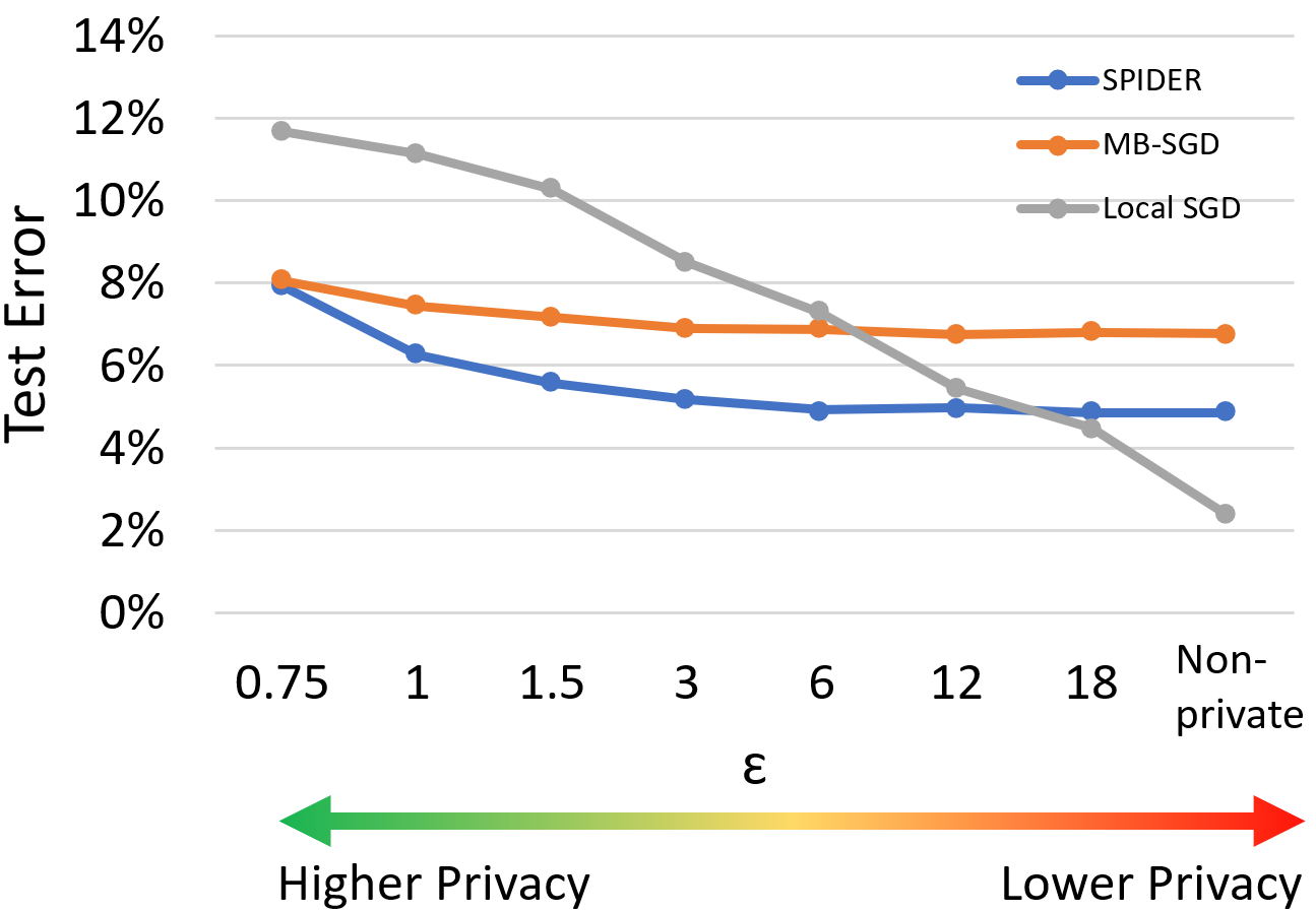
Figure 4: MNIST data. $M=25,R=25$.

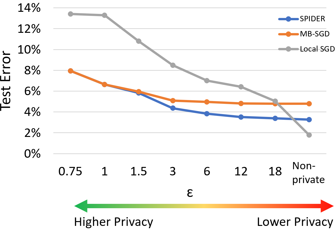
Figure 5: MNIST data. $M=12,R=50$.

Convolutional NN Classification with CIFAR-10: CIFAR-10 dataset (Krizhevsky et al., 2009) includes 10 image classes and we partition it into $N=10$ heterogeneous silos, each containing one class. Following (PyTorch team, ), we use a 5-layer CNN with two 5x5 convolutional layers (the first with 6 channels, the second with 16 channels, each followed by a ReLu activation and a 2x2 max pooling) and three fully connected layers with 120, 84, 10 neurons in each fully connected layer. The first and second fully connected layers are followed by a ReLu activation. As Figure 6 and Figure 7 show, ISRL-DP FedProx-SPIDER outperforms both ISRL-DP baselines for most tested privacy levels.

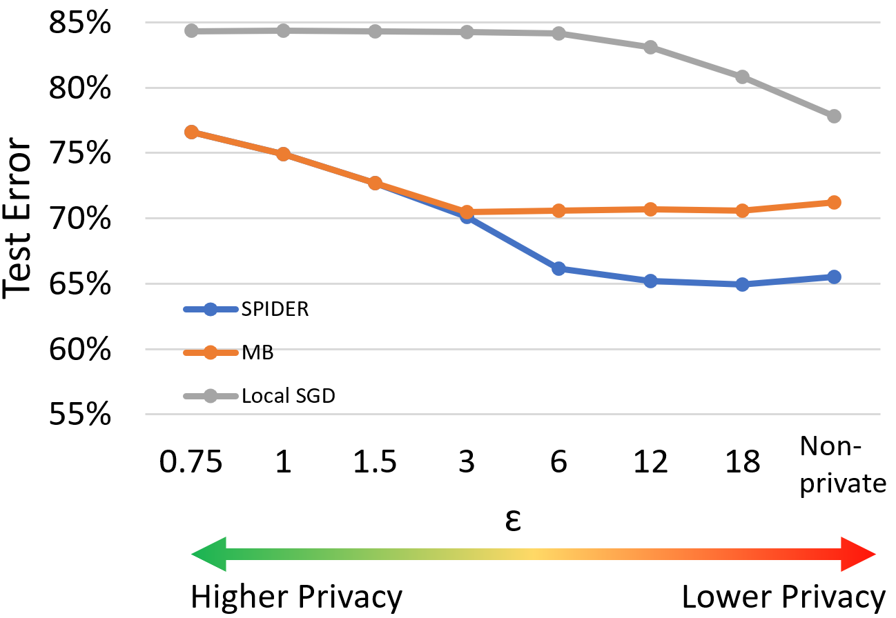
Figure 6: CIFAR-10 data. $M=10,R=50$.

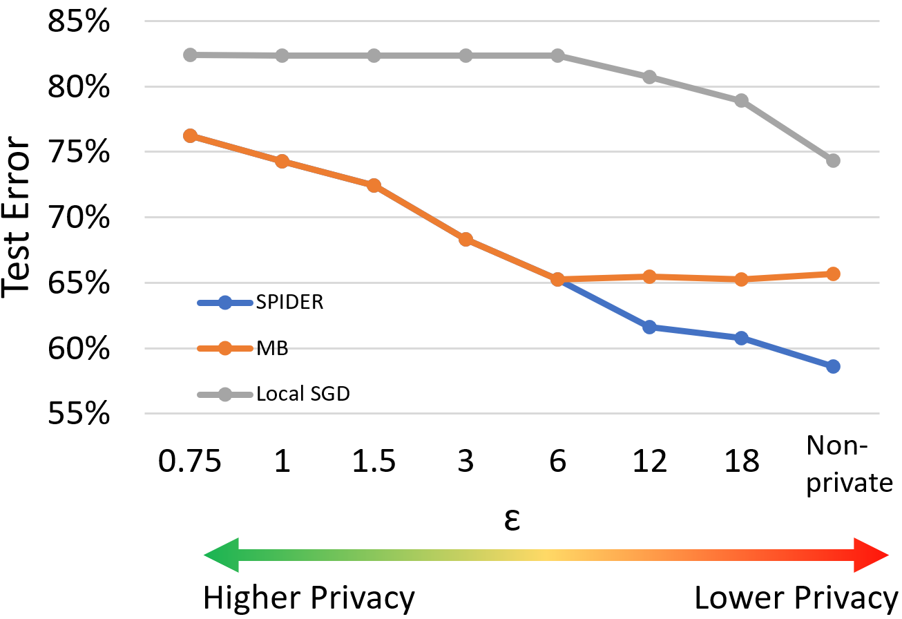
Figure 7: CIFAR-10 data. $M=10,R=100$.

Neural Net Classification with Breast Cancer Data: With the Wisconsin Breast Cancer (Diagnosis) (WBCD) dataset (Dua and Graff, 2017), our task is to diagnose breast cancers as malignant vs. benign. We partition the data set into $N=2$ heterogeneous silos, one containing malignant labels and the other benign labels. We use a 2-layer perceptron with 5 neurons in the hidden layer. As Figure 8 shows, ISRL-DP FedProx-SPIDER outperforms both ISRL-DP baselines for most tested privacy levels.

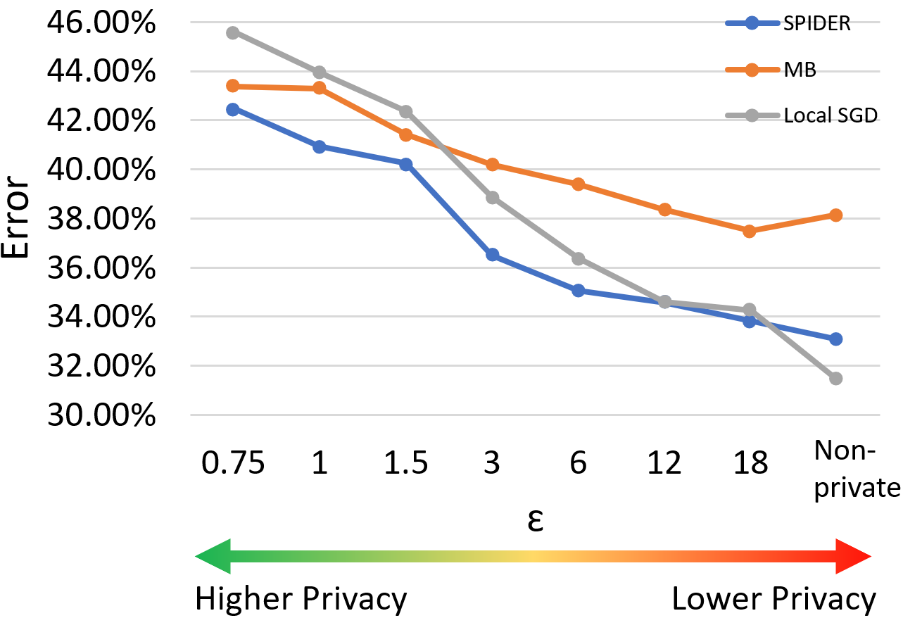
Figure 8: WBCD data. $M=2,R=25$.

5 CONCLUDING REMARKS AND OPEN QUESTIONS

We considered non-convex FL in the absence of trust in the server or other silos. We discussed the merits of ISRL-DP and SDP in this setting. For two broad classes of non-convex loss functions, we provided novel ISRL-DP/SDP FL algorithms and utility bounds that advance the state-of-the-art. For proximal-PL losses, our algorithms are nearly optimal and show that neither convexity or i.i.d. data is required to obtain fast rates. Numerical experiments demonstrated the practicality of our algorithm at providing both high accuracy and privacy on several learning tasks and data sets. An interesting open problem is proving tight bounds on the gradient norm for private non-convex FL. We discuss limitations and societal impacts of our work in Appendices I and J.

Acknowledgements

This work was supported in part with funding from the AFOSR Young Investigator Program award and a gift from the USC-Meta Center for Research and Education in AI and Learning.

SUPPLEMENTARY MATERIAL

Appendix A Inter-Silo Record Level Differential Privacy (ISRL-DP): Rigorous Definition

Let $\mathcal{A}$ be a randomized algorithm, where the silos communicate over $R$ rounds for their FL task. In each round of communication $r\in[R]$, each silo $i$ transmits a message $Z_{r}^{(i)}\in\mathcal{Z}$ (e.g. stochastic gradient) to the server or other silos, and the messages are aggregated. The transmitted message $Z_{r}^{(i)}$ is a (random) function of previously communicated messages and the data of user $i$; that is, $Z^{(i)}_{r}:=\mathcal{R}^{(i)}_{r}(\mathbf{Z}_{1:r-1},X_{i})$, where $\mathbf{Z}_{1:r-1}:=\{Z_{t}^{(j)}\}_{j\in[N],t\in[r-1]}$. The silo-level local privacy of $\mathcal{A}$ is completely characterized by the randomizers $\mathcal{R}^{(i)}_{r}:\mathcal{Z}^{(r-1)\times N}\times\mathcal{X}^{n_{i}}\to\mathcal{Z}$ ($i\in[N],~{}r\in[R]$). $\mathcal{A}$ is $(\epsilon,\delta)$-ISRL-DP if for all $i\in[N]$, the full transcript of silo $i$’s communications (i.e. the collection of all $R$ messages $\{Z^{(i)}_{r}\}_{r\in[R]}$) is $(\epsilon,\delta)$-DP, conditional on the messages and data of all other silos. We write $\mathcal{A}(\mathbf{X})\underset{(\epsilon,\delta)}{\simeq}\mathcal{A}(\mathbf{X}^{\prime})$ if 3 holds for all measurable subsets $S$.

Definition 4.

(Inter-Silo Record Level Differential Privacy) Let $\rho_{i}:\mathcal{X}^{2}\to[0,\infty)$, $\rho_{i}(X_{i},X^{\prime}_{i}):=\sum_{j=1}^{n}\mathds{1}_{\{x_{i,j}\neq x_{i,j}^{\prime}\}}$, $i\in[N]$. A randomized algorithm $\mathcal{A}:\mathcal{X}_{1}^{n}\times\cdots\times\mathcal{X}_{N}^{n}\to\mathcal{Z}^{R\times N}$ is $(\epsilon,\delta)$-ISRL-DP if for all $i\in[N]$ and all $\rho_{i}$-adjacent $X_{i},X_{i}^{\prime}\in\mathcal{X}^{n}$, we have $(\mathcal{R}^{(i)}_{1}(X_{i}),\mathcal{R}^{(i)}_{2}(\mathbf{Z}_{1},X_{i}),\cdots,\mathcal{R}^{(i)}_{R}(\mathbf{Z}_{1:R-1},X_{i}))\underset{(\epsilon,\delta)}{\simeq}(\mathcal{R}^{(i)}_{1}(X^{\prime}_{i}),\mathcal{R}^{(i)}_{2}(\mathbf{Z}^{\prime}_{1},X^{\prime}_{i}),\cdots,\mathcal{R}^{(i)}_{R}(\mathbf{Z}^{\prime}_{1:R-1},X^{\prime}_{i})),$ where $\mathbf{Z}_{r}:=\{\mathcal{R}^{(i)}_{r}(\mathbf{Z}_{1:r-1},X_{i})\}_{i=1}^{N}$ and $\mathbf{Z}^{\prime}_{r}:=\{\mathcal{R}^{(i)}_{r}(\mathbf{Z}^{\prime}_{1:r-1},X_{i}^{\prime})\}_{i=1}^{N}$.

Appendix B Relationships Between Notions of Differential Privacy

In this section, we collect a couple of facts about the relationships between different notions of DP, which were proved in ((Lowy and Razaviyayn, 2021b)). Suppose $\mathcal{A}$ is $(\epsilon,\delta)$-ISRL-DP. Then:

• $\mathcal{A}$ is $(\epsilon,\delta)$-CDP; and

• $\mathcal{A}$ is $(n\epsilon,ne^{(n-1)\epsilon}\delta)$-user-level DP.

Thus, if $\epsilon_{0}\lesssim 1/n$ and $\delta_{0}=o(1/n^{2})$, then any $(\epsilon_{0},\delta_{0})$-ISRL-DP algorithm also provides a meaningful $(\epsilon,\delta)$-user-level DP guarantee, with $\epsilon\lesssim 1$.

Appendix C Further Discussion of Related Work

DP Optimization with the Polyak-Łojasiewicz (PL) Condition: For unconstrained central DP optimization, ((Wang et al., 2017; Kang et al., 2021; Zhang et al., 2021)) provide bounds for Lipschitz losses satisfying the classical PL inequality. However, the combined assumptions of Lipschitzness and PL on $\mathbb{R}^{d}$ (unconstrained) are very strong and rule out most interesting PL losses, such as strongly convex, least squares, and neural nets, since the Lipschitz parameter $L$ of such losses is infinite or prohibitively large. We address this gap by considering the Proximal PL condition, which admits such interesting loss functions. There was no prior work on DP optimization (in particular, FL) with the Proximal PL condition.

DP Smooth Non-convex Distributed ERM: Non-convex federated ERM has been considered in previous works under stricter assumptions of smooth loss and (usually) a trusted server. ((Wang et al., 2019a)) provide state-of-the-art CDP upper bounds for distributed ERM of order $\mathbb{E}\|\nabla\widehat{F}_{\mathbf{X}}(w_{\text{priv}})\|^{2}\lesssim\left(\frac{\sqrt{d}}{\epsilon nN}\right)$ with perfect communication ($M=N$), relying on a trusted server (in conjunction with secure multi-party computation) to perturb the aggregated gradients. Similar bounds were attained by ((Noble et al., 2022)) for $M<N$ with a DP variation of SCAFFOLD ((Karimireddy et al., 2020)). In Theorem 3.2, we improve on these utility bound under the weaker trust model of shuffle DP (no trusted server) and with unreliable communication (i.e. arbitrary $M\in[N]$). We also improve over the state-of-the-art ISRL-DP bound of ((Noble et al., 2022)), in Theorem 3.1. A number of other works have also addressed private non-convex federated ERM (under various notions of DP), but have fallen short of the state-of-the-art utility and communication complexity bounds:

• The noisy FedAvg algorithm of ((Hu et al., 2021)) is not ISRL-DP for any $N>n$ since the variance of the Gaussian noise $\sigma^{2}\approx TKL^{2}\log(1/\delta)/nN\epsilon^{2}$ decreases as $N$ increases; moreover, for their prescribed stepsize $\eta=\frac{\sqrt{N}}{\sqrt{T}}$, the resulting rate (with $T=RK$) from ((Hu et al., 2021, Theorem 2)) is $\mathbb{E}\|\nabla\widehat{F}(\widehat{w}_{R})\|^{2}=\widetilde{O}\left(\frac{d\sqrt{NT}K}{\epsilon^{2}nN}+\frac{NK^{2}}{T}+\frac{\sqrt{N}}{\sqrt{T}}+\frac{dK^{2}}{\epsilon^{2}n}\right)$ which grows unbounded with $T$. Moreover, $T$ and $K$ are not specified in their work, so it is not clear what bound their algorithm is able to attain, or how many communication rounds are needed to attain it.

• Theorems 3 and 7 of ((Ding et al., 2021)) provide ISRL-DP upper bounds on the empirical gradient norm which hold for sufficiently large $R\geq T_{\min}^{\text{nc}}$ for some unspecified $T_{\min}^{\text{nc}}$. The resulting upper bounds are bigger than $\frac{d\sigma^{2}}{R^{1/3}}\approx\frac{dR^{2/3}}{\epsilon^{2}n^{2}}$. In particular, the bounds becomes trivial for large $R$ (diverges) and no utility bound expressed in terms of problem parameters (rather than unspecified design parameters $R$ or $T$) is provided. Also, no communication complexity bound is provided.

DP Smooth Non-convex Centralized ERM ($N=1$): In the centralized setting with a single client and smooth loss function, several works ((Zhang et al., 2017; Wang et al., 2017, 2019a; Arora et al., 2022)) have considered CDP (unconstrained) non-convex ERM (with gradient norm as the utility measure): the state-of-the-art bound is $\mathbb{E}\|\nabla\widehat{F}_{\mathbf{X}}(w_{\text{priv}})\|^{2}=\mathcal{O}\left(\frac{\sqrt{d\ln(1/\delta)}}{\epsilon n}\right)^{4/3}$ ((Arora et al., 2022)). Our private FedProx-SPIDER algorithms build on the DP SPIDER-Boost of ((Arora et al., 2022)), by parallelizing their updates for FL and incorporating proximal updates to cover non-smooth losses.

Non-private FL: In the absence of privacy constraints, there is a plethora of works studying the convergence of FL algorithms in both the convex ((Koloskova et al., 2020; Li et al., 2020b; Karimireddy et al., 2020; Woodworth et al., 2020a, b; Yuan and Ma, 2020)) and non-convex ((Li et al., 2020a; Zhang et al., 2020; Karimireddy et al., 2020)) settings. We do not attempt to provide a comprehensive survey of these works here; see ((Kairouz et al., 2019)) for such a survey. However, we briefly discuss some of the well known non-convex FL works:

• The “FedProx” algorithm of ((Li et al., 2020a)) augments FedAvg ((McMahan et al., 2017)) with a regularization term in order to decrease “client drift” in heterogeneous FL problems with smooth non-convex loss functions. (By comparison, we use a proximal term in our private algorithms to deal with non-smooth non-convex loss functions, and show that our algorithms effectively handle heterogeneous client data via careful analysis.)

• ((Zhang et al., 2020)) provides primal-dual FL algorithms for non-convex loss functions that have optimal communication complexity (in a certain sense).

• The SCAFFOLD algorithm of ((Karimireddy et al., 2020)) can be viewed as a hybrid between Local SGD (FedAvg) and MB-SGD, as ((Woodworth et al., 2020b)) observed. Convergence guarantees for their algorithm with non-convex loss functions are provided.

Appendix D Differential Privacy Building Blocks

Basic DP tools: We begin by reviewing the privacy guarantees of the Gaussian mechanism. The classical $(\epsilon,\delta)$-DP bounds for the Gaussian mechanism ((Dwork and Roth, 2014, Theorem A.1)) were only proved for $\epsilon\leq 1$, so we shall instead state the privacy guarantees in terms of zero-concentrated differential privacy (zCDP)–which should not be confused with central differential privacy (CDP)–and then convert these into $(\epsilon,\delta)$-DP guarantees. We first recall ((Bun and Steinke, 2016, Definition 1.1)):

Definition 5.

A randomized algorithm $\mathcal{A}:\mathcal{X}^{n}\to\mathcal{W}$ satisfies $\rho$-zero-concentrated differential privacy ($\rho$-zCDP) if for all $X,X^{\prime}\in\mathcal{X}^{n}$ differing in a single entry (i.e. $d_{\text{hamming}}(X,X^{\prime})=1$), and all $\alpha\in(1,\infty)$, we have

$$D_{\alpha}(\mathcal{A}(X)||\mathcal{A}(X^{\prime}))\leq\rho\alpha,$$

where $D_{\alpha}(\mathcal{A}(X)||\mathcal{A}(X^{\prime}))$ is the $\alpha$-Rényi divergence between the distributions of $\mathcal{A}(X)$ and $\mathcal{A}(X^{\prime})$.

zCDP is weaker than pure DP, but stronger than approximate DP in the following sense:

Proposition D.1.

((Bun and Steinke, 2016, Proposition 1.3)) If $\mathcal{A}$ is $\rho$-zCDP, then $\mathcal{A}$ is $(\rho+2\sqrt{\rho\log(1/\delta)},\delta)$ for any $\delta>0$. In particular, if $\epsilon\leq 2\ln(1/\delta)$, then any $\frac{\epsilon^{2}}{8\ln(1/\delta)}$-zCDP algorithm is $(\epsilon,\delta)$-DP.

The privacy guarantee of the Gaussian mechanism is as follows:

Proposition D.2.

((Bun and Steinke, 2016, Proposition 1.6)) Let $q:\mathcal{X}^{n}\to\mathbb{R}$ be a query with $\ell_{2}$-sensitivity $\Delta:=\sup_{X\sim X^{\prime}}\|q(X)-q(X^{\prime})\|$. Then the Gaussian mechanism, defined by $\mathcal{M}:\mathcal{X}^{n}\to\mathbb{R}$, $\mathcal{M}(X):=q(X)+u$ for $u\sim\mathcal{N}(0,\sigma^{2})$, is $\rho$-zCDP if $\sigma^{2}\geq\frac{\Delta^{2}}{2\rho}$. Thus, if $\epsilon\leq 2\ln(1/\delta)$ and $\sigma^{2}\geq\frac{4\Delta^{2}\ln(1/\delta)}{\epsilon^{2}}$, then $\mathcal{M}$ is $(\epsilon,\delta)$-DP.

Our multi-pass algorithms will also use advanced composition for their privacy analysis:

Theorem D.1.

((Dwork and Roth, 2014, Theorem 3.20)) Let $\epsilon\geq\ 0,\delta,\delta^{\prime}\in[0,1)$. Assume $\mathcal{A}_{1},\cdots,\mathcal{A}_{R}$, with $\mathcal{A}_{r}:\mathcal{X}^{n}\times\mathcal{W}\to\mathcal{W}$, are each $(\epsilon,\delta)$-DP  $\forall r=1,\cdots,R$. Then, the adaptive composition $\mathcal{A}(X):=\mathcal{A}_{R}(X,\mathcal{A}_{R-1}(X,\mathcal{A}_{R-2}(X,\cdots)))$ is $(\epsilon^{\prime},R\delta+\delta^{\prime})$-DP for $\epsilon^{\prime}=\sqrt{2R\ln(1/\delta^{\prime})}\epsilon+R\epsilon(e^{\epsilon}-1)$.

Note that the moments accountant ((Abadi et al., 2016)) provides a slightly tighter composition bound (by a logarithmic factor) and can be used instead of Theorem D.1 if one is concerned with logarithmic factors. We use the moments accountant for our numerical experiments: see Appendix H. Sometimes it is more convenient to analyze the compositional privacy guarantees of our algorithm through the lens of zCDP:

Lemma D.1.

((Bun and Steinke, 2016, Lemma 2.3)) Suppose $\mathcal{A}:\mathcal{X}^{n}\to\mathcal{Y}$ satisfies $\rho$-zCDP and $\mathcal{A}^{\prime}:\mathcal{X}^{n}\times\mathcal{Y}\to\mathcal{Z}$ satisfies $\rho^{\prime}$-zCDP (as a function of its first argument). Define the composition of $\mathcal{A}$ and $\mathcal{A}^{\prime}$, $\mathcal{A}^{\prime\prime}:\mathcal{X}^{n}\to\mathcal{Z}$ by $\mathcal{A}^{\prime\prime}(X)=\mathcal{A}^{\prime}(X,\mathcal{A}(X))$. Then $\mathcal{A}^{\prime\prime}$ satisfies $(\rho+\rho^{\prime})$-zCDP. In particular, the composition of $T$ $\rho$-zCDP mechanisms is a $T\rho$-zCDP mechanism.

Shuffle Private Vector Summation: Here we recall the shuffle private vector summation protocol $\mathcal{P}_{\text{vec}}$ of ((Cheu et al., 2021)), and its privacy and utility guarantee. First, we will need the scalar summation protocol, Algorithm 4. Both of Algorithm 4 and Algorithm 5 decompose into a local randomizer $\mathcal{R}$ that silos perform and an analyzer component $\mathcal{A}$ that the shuffler executes. Below we use $\mathcal{S}(\mathbf{y})$ to denote the shuffled vector $\mathbf{y}$: i.e. the vector with same dimension as $\mathbf{y}$ whose components are random permutations of the components of $\mathbf{y}$.

Algorithm 4 $\mathcal{P}_{\text{1D}}$, a shuffle protocol for summing scalars ((Cheu et al., 2021))

1:  Input: Scalar database $X=(x_{1},\cdots x_{N})\in[0,L]^{N}$; $g,b\in\mathbb{N};p\in(0,\frac{1}{2})$.

2:  procedure: Local Randomizer $\mathcal{R}_{1D}(x_{i})$

3:     $\widebar{x}_{i}\leftarrow\lfloor x_{i}g/L\rfloor$.

4:     Sample rounding value $\eta_{1}\sim\textbf{Ber}(x_{i}g/L-\widebar{x}_{i})$.

5:     Set $\hat{x}_{i}\leftarrow\widebar{x}_{i}+\eta_{1}$.

6:     Sample privacy noise value $\eta_{2}\sim\textbf{Bin}(b,p)$.

7:     Report $\mathbf{y}_{i}\in\{0,1\}^{g+b}$ containing $\hat{x}_{i}+\eta_{2}$ copies of $1$ and $g+b-(\hat{x}_{i}+\eta_{2})$ copies of $0$.

8:  end procedure

9:  procedure: Analyzer $\mathcal{A}_{\text{1D}}(\mathcal{S}(\mathbf{y}))$

10:     Output estimator $\frac{L}{g}((\sum_{i=1}^{N}\sum_{j=1}^{b+g}(\mathbf{y}_{i})_{j})-pbn)$.

11:  end procedure

The vector summation protocol Algorithm 5 invokes the scalar summation protocol, Algorithm 4, $d$ times. In the Analyzer procedure, we use $\mathbf{y}$ to denote the collection of all $Nd$ shuffled (and labeled) messages that are returned by the the local randomizer applied to all of the $N$ input vectors. Since the randomizer labels these messages by coordinate, $\mathbf{y}_{j}$ consists of $N$ shuffled messages labeled by coordinate $j$ (for all $j\in[d]$).

Algorithm 5 $\mathcal{P}_{\text{vec}}$, a shuffle protocol for vector summation ((Cheu et al., 2021))

1:  Input: database of $d$-dimensional vectors $\mathbf{X}=(\mathbf{x}_{1},\cdots,\mathbf{x}_{N}$); privacy parameters $\epsilon,\delta$; $L$.

2:  procedure: Local Randomizer $\mathcal{R}_{\text{vec}}(\mathbf{x}_{i})$

3:     for $j\in[d]$ do

4:        Shift component to enforce non-negativity: $\mathbf{w}_{i,j}\leftarrow\mathbf{x}_{i,j}+L$

5:        $\mathbf{m}_{j}\leftarrow\mathcal{R}_{1D}(\mathbf{w}_{i,j})$

6:     end for

7:     Output labeled messages $\{(j,\mathbf{m}_{j})\}_{j\in[d]}$

8:  end procedure

9:  procedure: Analyzer $\mathcal{A}_{\text{vec}}(\mathbf{y})$

10:     for $j\in[d]$ do

11:        Run analyzer on coordinate $j$’s messages $z_{j}\leftarrow\mathcal{A}_{\text{1D}}(\mathbf{y}_{j})$

12:        Re-center: $o_{j}\leftarrow z_{j}-L$

13:     end for

14:     Output the vector of estimates $\mathbf{o}=(o_{1},\cdots o_{d})$

15:  end procedure

When we use Algorithm 5 in our SDP FL algorithms, each of the $M_{r}=M$ available silos contributes $K$ messages, so $N=MK$ in the notation of Algorithm 5. Also, $x_{i}$ represents $K$ stochastic gradients, and available silos perform $\mathcal{R}_{\text{vec}}$ on each one (in parallel) before sending the collection of all of these randomized, discrete stochastic gradients–denoted $\mathcal{R}_{\text{vec}}(\mathbf{x}_{i})$–to the shuffler. The shuffler permutes the elements of $\mathcal{R}_{\text{vec}}(\mathbf{x}_{1}),\cdots\mathcal{R}_{\text{vec}}(\mathbf{x}_{M})$, then executes $\mathcal{A}_{\text{vec}}$, and sends $\frac{1}{M}\mathbf{o}$–which is a noisy estimate of the average stochastic gradient–to the server. When there is no confusion, we will sometimes hide input parameters other than $\mathbf{X}$ and denote $\mathcal{P}_{\text{vec}}(\mathbf{X}):=\mathcal{P}_{\text{vec}}(\mathbf{X};\epsilon,\delta;L)$. We now provide the privacy and utility guarantee of Algorithm 5:

Theorem D.2 (((Cheu et al., 2021))).

For any $0<\epsilon\leq 15,0<\delta<1/2,d,N\in\mathbb{N}$, and $L>0$, there are choices of parameters $b,g\in\mathbb{N}$ and $p\in(0,1/2)$ for $\mathcal{P}_{\text{1D}}$ (Algorithm 4) such that, for $\mathbf{X}=(\mathbf{x}_{1},\cdots\mathbf{x}_{N})$ containing vectors of maximum norm $\max_{i\in[N]}\|\mathbf{x}_{i}\|\leq L$, the following holds: 1) $\mathcal{P}_{\text{vec}}$ is $(\epsilon,\delta)$-SDP; and 2) $\mathcal{P}_{\text{vec}}(\mathbf{X})$ is an unbiased estimate of $\sum_{i=1}^{N}\mathbf{x}_{i}$ with bounded variance

$$\mathbb{E}\left[\left\|\mathcal{P}_{\text{vec}}(\mathbf{X};\epsilon,\delta;L)-\sum_{i=1}^{N}\mathbf{x}_{i}\right\|^{2}\right]=\mathcal{O}\left(\frac{dL^{2}\log^{2}\left(\frac{d}{\delta}\right)}{\epsilon^{2}}\right).$$

Appendix E Supplemental Material for Section 2: Proximal PL Loss Functions

E.1 Noisy Proximal Gradient Methods forProximal PL FL (SO) - Pseudocodes

Algorithm 6 ISRL-DP Noisy Distributed Proximal Gradient Method

1:  Input: $R\in\mathbb{N},X_{i}\in\mathcal{X}^{n}(i\in[N]),\sigma^{2}\geq 0,K\leq\frac{n}{R},w_{0}\in\mathbb{R}^{d}$.

2:  for $r\in\{0,1,\cdots,R-1\}$ do

3:     for $i\in S_{r}$ in parallel do

4:        Server sends global model $w_{r}$ to silo $i$.

5:        Silo $i$ draws $\{x_{i,j}^{r}\}_{j=1}^{K}$ uniformly from $X_{i}$ (without replacement) and noise $u_{i}\sim\mathcal{N}(0,\sigma^{2}\mathbf{I}_{d}).$

6:        Silo $i$ sends $\widetilde{g}_{r}^{i}:=\frac{1}{K}\sum_{j=1}^{K}\nabla f^{0}(w_{r},x_{i,j}^{r})+u_{i}$ to server.

7:     end for

8:     Server aggregates $\widetilde{g}_{r}:=\frac{1}{M_{r}}\sum_{i\in S_{r}}\widetilde{g}_{r}^{i}$.

9:     Server updates $w_{r+1}:=\texttt{{prox}}_{\frac{1}{2\beta}f^{1}}(w_{r}-\frac{1}{2\beta}\widetilde{g}_{r})$

10:  end for

11:  Output: $w_{R}$.

Algorithm 7 SDP Noisy Distributed Proximal Gradient Method

1:  Input: Number of rounds $R\in\mathbb{N}$, data sets $X_{i}\in\mathcal{X}^{n_{i}}$ for $i\in[N]$, loss function $f(w,x)=f^{0}(w,x)+f^{1}(w,x)$, privacy parameters $\epsilon,\delta$, local batch size $K\leq\frac{n}{R}$, $w_{0}\in\mathbb{R}^{d}$.

2:  for $r\in\{0,1,\cdots,R-1\}$ do

3:     for $i\in S_{r}$ in parallel do

4:        Server sends global model $w_{r}$ to silo $i$.

5:        Silo $i$ draws $K$ samples $\{x_{i,j}^{r}\}_{j=1}^{K}$ uniformly from $X_{i}$ (without replacement) and computes $\{\nabla f^{0}(w_{r},x_{i,j}^{r})\}_{j\in[K]}$.

6:     end for

7:     Server updates $\widetilde{g}_{r}:=\frac{1}{M_{r}K}\mathcal{P}_{\text{vec}}(\{\nabla f^{0}(w_{r},x_{i,j}^{r})\}_{i\in S_{r},j\in[K]};\frac{N}{2M}\epsilon,\delta;L)$ and $w_{r+1}:=\texttt{{prox}}_{\frac{1}{2\beta}f^{1}}(w_{r}-\frac{1}{\beta}\widetilde{g}_{r})$

8:  end for

9:  Output: $w_{R}$.

E.2 Proof of Theorem 2.1: Heterogeneous FL (SO)

First we provide a precise re-statement of the result, in which we assume $M_{r}=M$ is fixed, for convenience:

Theorem E.1 (Re-statement of Theorem 2.1).

Grant Assumption 1, Assumption 2, and  Assumption 4 for $K=\lfloor\frac{n}{R}\rfloor$ and $R$ specified below. Let $\epsilon\leq\min\{8\ln(1/\delta),15\},\delta\in(0,1/2)$, $n\geq\widetilde{\Omega}(\kappa)$. There is a choice of $\sigma^{2}$ such that:

1. ISRL-DP Prox-SGD is $(\epsilon,\delta)$-ISRL-DP and

$$\mathbb{E}F(w_{R})-F^{*}=\widetilde{\mathcal{O}}\left(\frac{L^{2}}{\mu}\left(\frac{\kappa^{2}d\ln(1/\delta)}{\epsilon^{2}n^{2}M}+\frac{\kappa}{Mn}\right)\right)$$ (6)

in $R=\left\lceil 2\kappa\ln\left(\frac{\mu\Delta}{L^{2}}\min\left\{Mn,\frac{\epsilon^{2}n^{2}M}{d\ln(1/\delta)}\right\}\right)\right\rceil$ communication rounds, where $\Delta\geq F(w_{0})-F^{*}$.
2. SDP Prox-SGD is $(\epsilon,\delta)$-SDP for $M\geq N\min(\epsilon/2,1)$, and

$$\mathbb{E}F(w_{R})-F^{*}=\widetilde{\mathcal{O}}\left(\frac{L^{2}}{\mu}\left(\frac{\kappa^{2}d\ln^{2}(d/\delta)}{\epsilon^{2}n^{2}N^{2}}+\frac{\kappa}{Mn}\right)\right)$$ (7)

in $R=\left\lceil 2\kappa\ln\left(\frac{\mu\Delta}{L^{2}}\min\left\{Mn,\frac{\epsilon^{2}n^{2}N^{2}}{d\ln(1/\delta)}\right\}\right)\right\rceil$ communication rounds.

Proof.

We prove part 1 first. Privacy: First, by independence of the Gaussian noise across silos, it is enough show that transcript of silo $i$’s interactions with the server is DP for all $i\in[N]$ (conditional on the transcripts of all other silos). Since the batches sampled by silo $i$ in each round are disjoint (as we sample without replacement), the parallel composition theorem of DP ((McSherry, 2009)) implies that it suffices to show that each round is $(\epsilon,\delta)$-ISRL-DP. Then by post-processing ((Dwork and Roth, 2014)), we just need to show that that the noisy stochastic gradient $\widetilde{g}_{r}^{i}$ in line 6 of the algorithm is $(\epsilon,\delta)$-DP. Now, the $\ell_{2}$ sensitivity of this stochastic gradient is bounded by $\Delta_{2}:=\sup_{|X_{i}\Delta X^{\prime}_{i}|\leq 2,w\in\mathcal{W}}\|\frac{1}{K}\sum_{j=1}^{K}\nabla f(w,x_{i,j})-\nabla f(w,x^{\prime}_{i,j})\|\leq 2L/K,$ by $L$-Lipschitzness of $f.$ Hence Proposition D.2 implies that $\widetilde{g}_{r}^{i}$ in line 6 of the algorithm is $(\epsilon,\delta)$-DP for $\sigma^{2}\geq\frac{8L^{2}\ln(1/\delta)}{\epsilon^{2}K^{2}}$. Therefore, ISRL-DP Prox-SGD is $(\epsilon,\delta)$-ISRL-DP.

Excess loss: Denote the stochastic approximation of $F$ in round $r$ by $\widehat{F}_{r}(w):=\frac{1}{MK}\sum_{i\in S_{r}}\sum_{j=1}^{K}f(w,x_{i,j}^{r})$, and $\widebar{u}_{r}:=\frac{1}{M}\sum_{i\in S_{r}}u_{i}\sim\mathcal{N}(0,\frac{\sigma^{2}}{M}\mathbf{I}_{d})$. By $\beta$-smoothness, we have

$$\mathbb{E}F(w_{r+1}) =\mathbb{E}\left[F^{0}(w_{r+1})+f^{1}(w_{r})+f^{1}(w_{r+1})-f^{1}(w_{r})\right]$$

$$\leq\mathbb{E}F(w_{r})+\mathbb{E}\left[\langle\nabla\widehat{F}_{r}^{0}(w_{r}),w_{r+1}-w_{r}\rangle+\frac{\beta}{2}\|w_{r+1}-w_{r}\|^{2}+f^{1}(w_{r+1})-f^{1}(w_{r})+\langle\widebar{u}_{r},w_{r+1}\rangle\right]$$

$$\;\;\;+\mathbb{E}\langle\nabla F^{0}(w_{r})-\nabla\widehat{F}_{r}^{0}(w_{r}),w_{r+1}-w_{r}\rangle-\mathbb{E}\langle\widebar{u}_{r},w_{r+1}\rangle$$ (8)

$$\leq\mathbb{E}F(w_{r})+\mathbb{E}\left[\langle\nabla\widehat{F}_{r}^{0}(w_{r}),w_{r+1}-w_{r}\rangle+\beta\|w_{r+1}-w_{r}\|^{2}+f^{1}(w_{r+1})-f^{1}(w_{r})+\langle\widebar{u}_{r},w_{r+1}\rangle\right]$$

$$\;\;\;-\langle\widebar{u}_{r},w_{r+1}\rangle+\mathbb{E}\left[\frac{1}{2\beta}\|\nabla F^{0}(w_{r})-\nabla\widehat{F}^{0}_{r}(w_{r})\|^{2}\right],$$ (9)

where we used Young’s inequality to bound

$$\mathbb{E}\langle\nabla F^{0}(w_{r})-\nabla\widehat{F}_{r}^{0}(w_{r}),w_{r+1}-w_{r}\rangle \leq\underbrace{\mathbb{E}\left[\frac{1}{2\beta}\|\nabla F^{0}(w_{r})-\nabla\widehat{F}^{0}_{r}(w_{r})\|^{2}\right]}_{ⓐ}+\mathbb{E}\left[\frac{\beta}{2}\|w_{r+1}-w_{r}\|^{2}\right]$$ (10)

in the last line above. We bound ⓐ as follows:

$$\mathbb{E}\left[\frac{1}{2\beta}\left\|\nabla F^{0}(w_{r})-\nabla\widehat{F}^{0}_{r}(w_{r})\right\|^{2}\right] =\frac{1}{2\beta}\mathbb{E}\left\|\frac{1}{MK}\sum_{i\in S_{r}}\sum_{j=1}^{K}\nabla F^{0}(w_{r})-\nabla f^{0}(w_{r},x_{i,j}^{r})\right\|^{2}$$ (11)

$$=\frac{1}{2\beta M^{2}K^{2}}\sum_{i\in S_{r}}\sum_{j=1}^{K}\mathbb{E}\|\nabla F^{0}(w_{r})-\nabla f^{0}(w_{r},x_{i,j}^{r})\|^{2}$$ (12)

$$\leq\frac{L^{2}}{\beta MK},$$ (13)

by independence of the data and $L$-Lipschitzness of $f^{0}$.

Next, we will bound $\mathbb{E}\left[\langle\nabla\widehat{F}_{r}^{0}(w_{r}),w_{r+1}-w_{r}\rangle+\beta\|w_{r+1}-w_{r}\|^{2}+f^{1}(w_{r+1})-f^{1}(w_{r})+\langle\widebar{u}_{r},w_{r+1}\rangle\right]$. Denote $H^{\text{priv}}_{r}(y):=\langle\widehat{F}_{r}^{0}(w_{r}),y-w_{r}\rangle+\beta\|y-w_{r}\|^{2}+f^{1}(y)-f^{1}(w_{r})+\langle\widebar{u}_{r},y\rangle$ and $H_{r}(y):=\langle\nabla\widehat{F}_{r}^{0}(w_{r}),y-w_{r}\rangle+\beta\|y-w_{r}\|^{2}+f^{1}(y)-f^{1}(w_{r})$ Note that $H_{r}$ and $H^{\text{priv}}_{r}$ are $2\beta$-strongly convex. Denote the minimizers of these two functions by $y_{*}$ and $y_{*}^{\text{priv}}$ respectively. Now, conditional on $w_{r},S_{r}$, and $\widebar{u}_{r}$, we claim that

$$H_{r}(y_{*}^{\text{priv}})-H_{r}(y_{*})\leq\frac{\|\widebar{u}_{r}\|^{2}}{2\beta}.$$ (14)

To prove 14, we will need the following lemma:

Lemma E.1 (((Lowy and Razaviyayn, 2021a))).

Let $H(y),h(y)$ be convex functions on some convex closed set $\mathcal{Y}\subseteq\mathbb{R}^{d}$ and suppose that $H(w)$ is $2\beta$-strongly convex. Assume further that $h$ is $L_{h}$-Lipschitz. Define $y_{1}=\arg\min_{y\in\mathcal{Y}}H(y)$ and $y_{2}=\arg\min_{y\in\mathcal{Y}}[H(y)+h(y)]$. Then $\|y_{1}-y_{2}\|_{2}\leq\frac{L_{h}}{2\beta}.$

We apply Lemma E.1 with $H(y):=H_{r}(y),~{}h(y):=\langle\widebar{u}_{r},y\rangle$, $L_{h}=\|\widebar{u}_{r}\|$, $y_{1}=y_{*}$, and $y_{2}=y_{*}^{\text{priv}}$ to get

$$\|y_{*}-y_{*}^{\text{priv}}\|\leq\frac{\|\widebar{u}_{r}\|}{2\beta}.$$

On the other hand,

$$H_{r}^{\text{priv}}(y_{*}^{\text{priv}})=H_{r}(y_{*}^{\text{priv}})+\langle\widebar{u}_{r},y_{*}^{\text{priv}}\rangle\leq H_{r}^{\text{priv}}(y_{*})=H_{r}(y_{*})+\langle\widebar{u}_{r},y_{*}\rangle.$$

Combining these two inequalities yields

$$H_{r}(y_{*}^{\text{priv}})-H_{r}(y_{*}) \leq\langle\widebar{u}_{r},y_{*}-y_{*}^{\text{priv}}\rangle$$

$$\leq\|\widebar{u}_{r}\|\|y_{*}-y_{*}^{\text{priv}}\|$$

$$\leq\frac{\|\widebar{u}_{r}\|^{2}}{\beta},$$ (15)

as claimed. Also, note that $w_{r+1}=y_{*}^{\text{priv}}$. Further, by Assumption 4, we know

$$\mathbb{E}H_{r}(y_{*}) =\mathbb{E}\min_{y}\left[\langle\nabla\widehat{F}_{r}^{0}(w_{r}),y-w_{r}\rangle+\beta\|y-w_{r}\|^{2}+f^{1}(y)-f^{1}(w_{r})\right]$$ (16)

$$\leq-\frac{\mu}{2\beta}\mathbb{E}[\widehat{F}_{r}(w_{r})-\min_{w}\widehat{F}_{r}(w)]\leq-\frac{\mu}{2\beta}[F(w_{r})-F^{*}].$$ (17)

Combining this with 14, we get:

$$\mathbb{E}\left[\langle\nabla\widehat{F}_{r}^{0}(w_{r}),w_{r+1}-w_{r}\rangle+\beta\|w_{r+1}-w_{r}\|^{2}+f^{1}(w_{r+1})-f^{1}(w_{r})+\langle\widebar{u}_{r},w_{r+1}\rangle\right]$$

$$=\mathbb{E}H_{r}^{\text{priv}}(y_{*}^{\text{priv}})$$

$$=\mathbb{E}H_{r}(y_{*}^{\text{priv}})+\mathbb{E}\langle\widebar{u}_{r},w_{r+1}\rangle$$

$$\leq\mathbb{E}H_{r}(y_{*})+\frac{d\sigma^{2}}{\beta M}+\mathbb{E}\langle\widebar{u}_{r},w_{r+1}\rangle$$

$$\leq-\mathbb{E}\frac{\mu}{2\beta}[F(w_{r})-F^{*}]+\frac{d\sigma^{2}}{\beta M}+\mathbb{E}\langle\widebar{u}_{r},w_{r+1}\rangle.$$

Plugging the above bounds back into 9, we obtain

$$\mathbb{E}F(w_{r+1})\leq\mathbb{E}F(w_{r})-\frac{\mu}{2\beta}\mathbb{E}[F(w_{r})-F^{*}]+\frac{2d\sigma^{2}}{\beta M}+\frac{2L^{2}}{\beta MK},$$ (18)

whence

$$\mathbb{E}[F(w_{r+1})-F^{*}]\leq\mathbb{E}[F(w_{r})-F^{*}]\left(1-\frac{\mu}{2\beta}\right)+\frac{2d\sigma^{2}}{\beta M}+\frac{2L^{2}}{\beta MK}.$$ (19)

Using 19 recursively and plugging in $\sigma^{2}$, we get

$$\mathbb{E}[F(w_{R})-F^{*}]\leq\Delta\left(1-\frac{\mu}{2\beta}\right)^{R}+\frac{L^{2}}{\mu}\left[\frac{16d\ln(1/\delta)}{\epsilon^{2}K^{2}M}+\frac{1}{MK}\right].$$ (20)

Finally, plugging in $K$ and $R$, and observing that $\frac{1}{\ln\left(\frac{\beta}{\beta-\mu}\right)}\leq\kappa$, we conclude

$$\mathbb{E}F(w_{R})-F^{*}\lesssim\frac{L^{2}}{\mu}\left[\ln^{2}\left(\frac{\mu\Delta}{L^{2}}\min\left\{Mn,\frac{\epsilon^{2}n^{2}M}{d}\right\}\right)\left(\frac{\kappa^{2}d\ln(1/\delta)}{\epsilon^{2}n^{2}M}+\frac{\kappa}{Mn}\right)\right].$$

Next, we move to part 2.
Privacy: Since the batches used in each iteration are disjoint by our sampling (without replacement) strategy, the parallel composition theorem ((McSherry, 2009)) implies that it is enough to show that each of the $R$ rounds is $(\epsilon,\delta)$-SDP. This follows immediately from Theorem D.2 and privacy amplification by subsambling ((Ullman, 2017)) (silos only): in each round, the network “selects” a uniformly random subset of $M_{r}=M$ silos out of $N$, and the shuffler executes a $(\frac{N}{2M}\epsilon,\delta)$-DP (by $L$-Lipschitzness of $f^{0}(\cdot,x)\forall x\in\mathcal{X}$) algorithm $\mathcal{P}_{\text{vec}}$ on the data of these $M$ silos (line 8), implying that each round is $(\epsilon,\delta)$-SDP.

Utility: The proof is very similar to the proof of part 1, except that the variance of the Gaussian noise $\frac{d\sigma^{2}}{M}$ is replaced by the variance of $\mathcal{P}_{\text{vec}}$. Denoting $Z:=\frac{1}{MK}\mathcal{P}_{\text{vec}}(\{\nabla f^{0}(w_{r},x_{i,j}^{r})\}_{i\in S_{r},j\in[K]};\frac{N}{2M}\epsilon,\delta)-\frac{1}{MK}\sum_{i\in S_{r+1}}\sum_{j=1}^{K}\nabla f^{0}(w_{r},x_{i,j}^{r})$, we have (by Theorem D.2)

$$\mathbb{E}\|Z\|^{2}=\mathcal{O}\left(\frac{dL^{2}\ln^{2}(d/\delta)}{M^{2}K^{2}(\frac{N}{2M}\epsilon)^{2}}\right)=\mathcal{O}\left(\frac{dL^{2}\ln^{2}(d/\delta)}{\epsilon^{2}K^{2}N^{2}}\right).$$

Also, $Z$ is independent of the data and gradients. Hence we can simply replace $\frac{d\sigma^{2}}{M}$ by $\mathcal{O}\left(\frac{dL^{2}\ln^{2}(d/\delta)}{\epsilon^{2}K^{2}N^{2}}\right)$ and follow the same steps as the proof of Theorem 2.1. This yields (c.f. 19)

$$\mathbb{E}[F(w_{r+1})-F^{*}]\leq\mathbb{E}[F(w_{r})-F^{*}]\left(1-\frac{\mu}{2\beta}\right)+\mathcal{O}\left(\frac{dL^{2}\ln^{2}(d/\delta)}{\epsilon^{2}K^{2}N^{2}}\right)+\frac{2L^{2}}{\beta MK}.$$ (21)

Using 21 recursively, we get

$$\mathbb{E}[F(w_{R})-F^{*}]\leq\Delta\left(1-\frac{\mu}{2\beta}\right)^{R}+\frac{L^{2}}{\mu}\left[\mathcal{O}\left(\frac{dL^{2}\ln^{2}(d/\delta)}{\epsilon^{2}K^{2}N^{2}}\right)+\frac{1}{MK}\right].$$ (22)

Finally, plugging in $R$ and $K=n/R$, and observing that $\frac{1}{\ln\left(\frac{\beta}{\beta-\mu}\right)}\leq\kappa$, we conclude

$$\mathbb{E}F(w_{R})-F^{*}\lesssim\frac{L^{2}}{\mu}\left[\ln^{2}\left(\frac{\mu\Delta}{L^{2}}\min\left\{Mn,\frac{\epsilon^{2}n^{2}N^{2}}{d}\right\}\right)\left(\frac{\kappa^{2}d\ln^{2}(d/\delta)}{\epsilon^{2}n^{2}M}+\frac{\kappa}{Mn}\right)\right].$$

∎

E.3 SDP Noisy Distributed Prox-PL SVRG Pseudocode

Our SDP Prox-SVRG algorithm is described in Algorithm 8.

Algorithm 8 SDP Prox-SVRG $(w_{0},E,K,\eta,\epsilon,\delta)$

1:  Input: Number of epochs $E\in\mathbb{N}$, local batch size $K\in[n]$, epoch length $Q=\lfloor\frac{n}{K}\rfloor$, data sets $X_{i}\in\mathcal{X}^{n}$, loss function $f(w,x)=f^{0}(w,x)+f^{1}(w)$, step size $\eta$, privacy parameters $\epsilon,\delta$, initial parameters $\widebar{w}_{0}=w_{0}^{Q}=w_{0}\in\mathbb{R}^{d}$; $\mathcal{P}_{\text{vec}}$ privacy parameters $\widetilde{\epsilon}:=\frac{\epsilon Nn}{8MK\sqrt{4EQ\ln(2/\delta)}}$ and $\widetilde{\delta}:=\frac{\delta}{2EQ}$.

2:  for $r\in\{0,1,\cdots,E-1\}$ do

3:     Server updates $w^{0}_{r+1}=w^{Q}_{r}$.

4:     for $i\in S_{r}$ in parallel do

5:        Server sends global model $w_{r}$ to silo $i$.

6:        silo $i$ computes $\{\nabla f^{0}(\widebar{w}_{r},x_{i,j})\}_{j=1}^{n}$.

7:        Server updates $\widetilde{g}_{r+1}:=\frac{1}{M_{r+1}n}\mathcal{P}_{\text{vec}}(\{\nabla f^{0}(\widebar{w}_{r},x_{i,j})\}_{i\in S_{r+1},j\in[n]};\widetilde{\epsilon},\widetilde{\delta};L)$.

8:        for $t\in\{0,1,\cdots Q-1\}$ do

9:           silo $i$ draws $\{x_{i,j}^{r+1,t}\}_{j=1}^{K}$ uniformly from $X_{i}$ with replacement, and computes $\{\nabla f^{0}(w_{r+1}^{t},x_{i,j}^{r+1,t})\}_{j=1}^{K}$.

10:           Server updates $\widetilde{p}_{r+1}^{t}:=\frac{1}{M_{r+1}K}\mathcal{P}_{\text{vec}}(\{\nabla f^{0}(w_{r+1}^{t},x_{i,j}^{r+1,t})-\nabla f^{0}(\widebar{w}_{r+1},x_{i,j}^{r+1,t})\}_{i\in S_{r+1},j\in[K]};\widetilde{\epsilon},\widetilde{\delta};2L)$

11:           Server updates $\widetilde{v}_{r+1}^{t}:=\widetilde{p}_{r+1}^{t}+\widetilde{g}_{r+1}$ and $w_{r+1}^{t+1}:=\texttt{{prox}}_{\eta f^{1}}(w_{r+1}^{t}-\eta\widetilde{v}_{r+1}^{t})$.

12:        end for

13:        Server updates $\widebar{w}_{r+1}:=w_{r+1}^{Q}$.

14:     end for

15:  end for

16:  Output: $w_{\text{priv}}\sim\text{Unif}(\{w_{r+1}^{t}\}_{r=0,1,\cdots,E-1;t=0,1,\cdots Q-1})$.

Algorithm 9 SDP Prox-PL-SVRG

1:  for $s\in[S]$ do

2:     $w_{s}=\texttt{SDP Prox-SVRG}(w_{s-1},E,K,\eta,\frac{\epsilon}{2\sqrt{2S}},\frac{\delta}{2S})$.

3:  end for

4:  Output: $w_{\text{priv}}:=w_{S}$.

E.4 Proof of Theorem 2.2: Federated ERM

For the precise/formal version of Theorem 2.2, we will need an additional notation: the heterogeneity parameter $\upsilon_{\mathbf{X}}^{2}$, which has appeared in other works on FL (e.g. ((Woodworth et al., 2020b))). Assume:

Assumption 5.

$\frac{1}{N}\sum_{i=1}^{N}\|\nabla\widehat{F}^{0}_{i}(w)-\nabla\widehat{F}^{0}_{\mathbf{X}}(w)\|^{2}\leq\hat{\upsilon}_{\mathbf{X}}^{2}$ for all $i\in[N],~{}w\in\mathcal{W}$.

Additionally, motivated by practical FL considerations (especially cross-device FL ((Kairouz et al., 2019))), we shall actually prove a more general result, which holds even when the number of active silos in each round is random:

Assumption 6.

In each round $r$, a uniformly random subset $S_{r}$ of $M_{r}\in[N]$ silos can communicate with the server, where $\{M_{r}\}_{r\geq 0}$ are independent with $\frac{1}{M}:=\mathbb{E}(\frac{1}{M_{r}})$.

We will require the following two lemmas for the proofs in this Appendix section:

Lemma E.2 (((J Reddi et al., 2016))).

Let $\widehat{F}(w)=\widehat{F}^{0}(w)+f^{1}(w)$, where $\widehat{F}^{0}$ is $\beta$-smooth and $f^{1}$ is proper, closed, and convex. Let $y:=\texttt{{prox}}_{\eta f^{1}}(w-\eta d^{\prime})$ for some $d^{\prime}\in\mathbb{R}^{d}$. Then for all $z\in\mathbb{R}^{d}$, we have:

$$\widehat{F}(y)\leq\widehat{F}(z)+\langle y-z,\nabla\widehat{F}^{0}(w)-d^{\prime}\rangle+\left[\frac{\beta}{2}-\frac{1}{2\eta}\right]\|y-w\|^{2}+\left[\frac{\beta}{2}+\frac{1}{2\eta}\right]\|z-w\|^{2}-\frac{1}{2\eta}\|y-z\|^{2}.$$

Lemma E.3.

For all $t\in\{0,1,\cdots,Q-1\}$ and $r\in\{0,1,\cdots,E-1\}$, the iterates of Algorithm 1 satisfy:

$$\mathbb{E}\|\nabla\widehat{F}^{0}(w_{r+1}^{t})-\widetilde{v}_{r+1}^{t}\|^{2}\leq\frac{8\mathds{1}_{\{MK<Nn\}}}{MK}\beta^{2}\mathbb{E}\|w_{r+1}^{t}-\widebar{w}_{r}\|^{2}+\frac{2(N-M)\hat{\upsilon}_{\mathbf{X}}^{2}}{M(N-1)}\mathds{1}_{\{N>1\}}+\frac{d(\sigma_{1}^{2}+\sigma_{2}^{2})}{M}.$$

Moreover, the iterates of Algorithm 8 satisfy

$$\mathbb{E}\|\nabla\widehat{F}^{0}(w_{r+1}^{t})-\widetilde{v}_{r+1}^{t}\|^{2}\leq\frac{8\mathds{1}_{\{MK<Nn\}}}{MK}\beta^{2}\mathbb{E}\|w_{r+1}^{t}-\widebar{w}_{r}\|^{2}+\frac{2(N-M)\hat{\upsilon}_{\mathbf{X}}^{2}}{M(N-1)}\mathds{1}_{\{N>1\}}+\mathcal{O}\left(\frac{dL^{2}R\ln^{2}(dR/\delta)\ln(1/\delta)}{\epsilon^{2}n^{2}N^{2}}\right),$$

where $R=EQ$.

Proof.

We begin with the first claim (Algorithm 1). Denote

$$\zeta_{r+1}^{t} :=\frac{1}{M_{r+1}K}\sum_{i\in S_{r+1}}\sum_{j=1}^{K}[\underbrace{\nabla f^{0}(w_{r+1}^{t},x_{i,j}^{r+1,t})-\nabla f^{0}(\widebar{w}_{r},x_{i,j}^{r+1,t})}_{:=\zeta_{r+1}^{t,i,j}}]$$

$$=\widetilde{v}_{r+1}^{t}-\widetilde{g}_{r+1}-\widebar{u}_{2},$$

where $\widetilde{g}_{r+1}:=\frac{1}{M_{r+1}}\sum_{i\in S_{r+1}}\widetilde{g}^{i}_{r+1}=\frac{1}{M_{r+1}}\sum_{i\in S_{r+1}}\nabla\widehat{F}^{0}_{i}(\widebar{w}_{r})+\widebar{u}_{1}$, and $\widebar{u}_{j}=\frac{1}{M_{r+1}}\sum_{i\in S_{r+1}}u^{i}_{j}$ for $j=1,2$. Note $\mathbb{E}\zeta_{r+1}^{t,i,j}=\nabla\widehat{F}^{0}_{i}(w_{r+1}^{t})-\nabla\widehat{F}^{0}_{i}(\widebar{w}_{r})$. Then, conditional on all iterates through $w_{r+1}^{t}$ and $\widebar{w}_{r}$, we have:

$$\mathbb{E}\left\|\nabla\widehat{F}^{0}(w_{r+1}^{t})-\widetilde{v}_{r+1}^{t}\right\|^{2} =\mathbb{E}\left\|\frac{1}{M_{r+1}K}\sum_{i\in S_{r+1}}\sum_{j=1}^{K}[\zeta_{r+1}^{t,i,j}+\widetilde{g}_{r+1}^{i}-\nabla\widehat{F}^{0}(w_{r+1}^{t})]+\widebar{u}_{2}\right\|^{2}$$ (23)

$$=\mathbb{E}\left\|\frac{1}{M_{r+1}K}\sum_{i\in S_{r+1}}\sum_{j=1}^{K}[\zeta_{r+1}^{t,i,j}+\nabla\widehat{F}^{0}_{i}(\widebar{w}_{r})+u_{1}^{i}-\nabla\widehat{F}^{0}(w_{r+1}^{t})]+\widebar{u}_{2}\right\|^{2}$$ (24)

$$=\frac{d(\sigma_{1}^{2}+\sigma_{2}^{2})}{M}+\underbrace{\mathbb{E}\left\|\frac{1}{M_{r+1}K}\sum_{i\in S_{r+1}}\sum_{j=1}^{K}[\zeta_{r+1}^{t,i,j}+\nabla\widehat{F}^{0}_{i}(\widebar{w}_{r})-\nabla\widehat{F}^{0}(w_{r+1}^{t})]\right\|^{2}}_{:=ⓐ},$$ (25)

by independence of the Gaussian noise and the gradients. Now,

$$ⓐ =\mathbb{E}\left\|\frac{1}{M_{r+1}K}\sum_{i\in S_{r+1}}\sum_{j=1}^{K}\left\{[\zeta_{r+1}^{t,i,j}-\mathbb{E}\zeta_{r+1}^{t,i,j}]+\nabla\widehat{F}^{0}_{i}(w_{r+1}^{t})-\nabla\widehat{F}^{0}(w_{r+1}^{t})\right\}\right\|^{2}$$ (26)

$$\leq 2\mathbb{E}\left\|\frac{1}{M_{r+1}K}\sum_{i\in S_{r+1}}\sum_{j=1}^{K}\zeta_{r+1}^{t,i,j}-\mathbb{E}\zeta_{r+1}^{t,i,j}\right\|^{2}+2\mathbb{E}\left\|\frac{1}{M_{r+1}K}\sum_{i\in S_{r+1}}\sum_{j=1}^{K}\nabla\widehat{F}^{0}_{i}(w_{r+1}^{t})-\nabla\widehat{F}^{0}(w_{r+1}^{t})\right\|^{2}.$$ (27)

We bound the first term (conditional on $M_{r+1}$ and all iterates through round $r$) in 27 using Lemma F.2:

$$\mathbb{E}\left\|\frac{1}{M_{r+1}K}\sum_{i\in S_{r+1}}\sum_{j=1}^{K}\zeta_{r+1}^{t,i,j}-\mathbb{E}\zeta_{r+1}^{t,i,j}\right\|^{2} \leq\frac{\mathds{1}_{\{M_{r+1}K<Nn\}}}{M_{r+1}KNn}\sum_{i=1}^{N}\sum_{j=1}^{n}\mathbb{E}\left\|\zeta_{r+1}^{t,i,j}-\mathbb{E}\zeta_{r+1}^{t,i,j}\right\|^{2}$$

$$\leq\frac{\mathds{1}_{\{M_{r+1}K<Nn\}}}{MKNn}\sum_{i=1}^{N}\sum_{j=1}^{n}2\mathbb{E}\left[\left\|\nabla f^{0}(w_{r+1}^{t},x_{i,j}^{r+1,t})-f^{0}(\widebar{w}_{r},x_{i,j}^{r+1,t})\right\|^{2}\right]$$

$$\;\;\;+\mathbb{E}\|\nabla\widehat{F}^{0}(w_{r+1}^{t})-\nabla\widehat{F}^{0}(\widebar{w}_{r})\|^{2}$$

$$\leq\frac{4\mathds{1}_{\{M_{r+1}K<Nn\}}}{M_{r+1}K}\beta^{2}\|w_{r+1}^{t}-\widebar{w}_{r}\|^{2},$$

where we used Cauchy-Schwartz and $\beta$-smoothness in the second and third inequalities. Now if $M=N$, then $M_{r+1}=N$ (with probability $1$) and taking expectation with respect to $M_{r+1}$ (conditional on the $w$’s) bounds the left-hand side by $\frac{4\mathds{1}_{\{K<n\}}}{MK}\beta^{2}\|w_{r+1}^{t}-\widebar{w}_{r}\|^{2}=\frac{4\mathds{1}_{\{MK<Nn\}}}{MK}\beta^{2}\|w_{r+1}^{t}-\widebar{w}_{r}\|^{2}$, via Assumption 6. On the other hand, if $M<N$, then taking expectation with respect to $M_{r+1}$ (conditional on the $w$’s) bounds the left-hand-side by $\frac{4}{MK}\beta^{2}\|w_{r+1}^{t}-\widebar{w}_{r}\|^{2}=\frac{4\mathds{1}_{\{MK<Nn\}}}{MK}\beta^{2}\|w_{r+1}^{t}-\widebar{w}_{r}\|^{2}$ (since the indicator is always equal to $1$ if $M<N$). In either case, taking total expectation with respect to $\widebar{w}_{r},w_{r+1}^{t}$ yields

$$\mathbb{E}\left\|\frac{1}{M_{r+1}K}\sum_{i\in S_{r+1}}\sum_{j=1}^{K}\zeta_{r+1}^{t,i,j}-\mathbb{E}\zeta_{r+1}^{t,i,j}\right\|^{2}\leq\frac{4\mathds{1}_{\{MK<Nn\}}}{MK}\beta^{2}\mathbb{E}\|w_{r+1}^{t}-\widebar{w}_{r}\|^{2}.$$

We can again invoke Lemma F.2 to bound (conditional on $M_{r+1}$ and $w_{r+1}^{t}$) the second term in 27:

$$\mathbb{E}\left\|\frac{1}{M_{r+1}K}\sum_{i\in S_{r+1}}\sum_{j=1}^{K}\nabla\widehat{F}^{0}_{i}(w_{r+1}^{t})-\nabla\widehat{F}^{0}(w_{r+1}^{t})\right\|^{2} \leq\mathds{1}_{\{N>1\}}\frac{N-M_{r+1}}{(N-1)M_{r+1}}\times\frac{1}{N}\sum_{i=1}^{N}\|\nabla\widehat{F}^{0}_{i}(w_{r+1}^{t})-\nabla\widehat{F}^{0}(w_{r+1}^{t})\|^{2}$$

$$\leq\mathds{1}_{\{N>1\}}\frac{N-M_{r+1}}{(N-1)M_{r+1}}\hat{\upsilon}_{\mathbf{X}}^{2}.$$

Taking total expectation and combining the above pieces completes the proof of the first claim.

The second claim is very similar, except that the Gaussian noise terms $\widebar{u}_{1}$ and $\widebar{u}_{2}$ get replaced by the respective noises due to $\mathcal{P}_{\text{vec}}$: $Z_{1}:=\frac{1}{Mn}\mathcal{P}_{\text{vec}}(\{\nabla f^{0}(\widebar{w}_{r},x_{i,j})\}_{i\in S_{r+1},j\in[n]};\widetilde{\epsilon},\widetilde{\delta})-\frac{1}{M}\sum_{i\in S_{r+1}}\nabla\widehat{F}_{i}^{0}(\widebar{w}_{r})$ and $Z_{2}:=\frac{1}{MK}\left[\mathcal{P}_{\text{vec}}(\{\nabla f^{0}(w_{r+1}^{t},x_{i,j}^{r+1,t})-\nabla f^{0}(\widebar{w}_{r+1},x_{i,j}^{r+1,t})\}_{i\in S_{r+1},j\in[K]};\widetilde{\epsilon},\widetilde{\delta})-\sum_{i\in S_{r+1}}\sum_{j=1}^{K}(\nabla f^{0}(w_{r+1}^{t},x_{i,j}^{r+1,t})-f^{0}(\widebar{w}_{r},x_{i,j}^{r+1,t})\right]$.
By Theorem D.2, we have

$$\mathbb{E}\|Z_{1}\|^{2}=\mathcal{O}\left(\frac{dL^{2}\ln^{2}(d/\widetilde{\delta})}{M^{2}n^{2}\widetilde{\epsilon}^{2}}\right)=\mathcal{O}\left(\frac{dL^{2}R\ln^{2}(dR/\delta)\ln(1/\delta)}{\epsilon^{2}n^{2}N^{2}}\right)$$

and

$$\mathbb{E}\|Z_{2}\|^{2}=\mathcal{O}\left(\frac{dL^{2}\ln^{2}(d/\widetilde{\delta})}{M^{2}K^{2}\widetilde{\epsilon}^{2}}\right)=\mathcal{O}\left(\frac{dL^{2}R\ln^{2}(dR/\delta)\ln(1/\delta)}{\epsilon^{2}n^{2}N^{2}}\right).$$

∎

Below we provide a precise re-statement of Theorem 2.2 for $M<N$, including choices of algorithmic parameter.

Theorem E.2 (Complete Statement of Theorem 2.2).

Assume $\epsilon\leq\min\{2\ln(2/\delta),15\}$ and let $R:=EQ$. Suppose $\widehat{F}_{\mathbf{X}}$ is $\mu$-PPL and grant Assumption 1,  Assumption 2,  Assumption 6, and Assumption 5. Then:
1. Algorithm 2 is $(\epsilon,\delta)$-ISRL-DP if $\sigma_{1}^{2}=\frac{256L^{2}SE\log(2/\delta)\log(5E/\delta)}{\epsilon^{2}n^{2}}$, $\sigma_{2}^{2}=\frac{1024L^{2}SR\log(2/\delta)\log(2.5R/\delta)}{\epsilon^{2}n^{2}}$, and $K\geq\frac{\epsilon n}{4\sqrt{2SR\ln(2/\delta)}}$. Further, if $K\geq\left(\frac{n^{2}}{M}\right)^{1/3}$, $R=12\kappa$, and $S\geq\log_{2}\left(\frac{\hat{\Delta}_{\mathbf{X}}\mu M\epsilon^{2}n^{2}}{\kappa dL^{2}}\right)$, then there is $\eta$ such that $\forall\mathbf{X}\in\mathbb{X}$,

$$\mathbb{E}\widehat{F}_{\mathbf{X}\normalsize}(w_{S})-\widehat{F}_{\mathbf{X}\normalsize}^{*}=\widetilde{\mathcal{O}}\left(\kappa\frac{L^{2}d\ln(1/\delta)}{\mu\epsilon^{2}n^{2}M}+\frac{(N-M)\hat{\upsilon}_{\mathbf{X}}^{2}}{M(N-1)}\mathds{1}_{\{N>1\}}\right)$$

in $\widetilde{\mathcal{O}}(\kappa)$ communications.
2. Algorithm 8 is $(\epsilon,\delta)$-SDP, provided $M_{r+1}=M\geq\min\left\{\frac{(\epsilon NL)^{3/4}(d\ln^{3}(d/\delta))^{3/8}}{n^{1/4}(\beta\hat{\Delta}_{\mathbf{X}})^{3/8}},N\right\}$ for all $r$. Further, if $K\geq\left(\frac{n^{2}}{M}\right)^{1/3}$, $R=12\kappa$, and $S\geq\log_{2}\left(\frac{\hat{\Delta}_{\mathbf{X}}\mu\epsilon^{2}N^{2}n^{2}}{\kappa dL^{2}}\right)$, then there is $\eta$ such that $\forall\mathbf{X}\in\mathbb{X}$,

$$\mathbb{E}\widehat{F}_{\mathbf{X}\normalsize}(w_{S})-\widehat{F}_{\mathbf{X}\normalsize}^{*}=\widetilde{\mathcal{O}}\left(\kappa\frac{L^{2}d\ln(1/\delta)}{\mu\epsilon^{2}n^{2}N^{2}}+\frac{(N-M)\hat{\upsilon}_{\mathbf{X}}^{2}}{\mu M(N-1)}\mathds{1}_{\{N>1\}}\right).$$

Proof.

1. Privacy: For simplicity, assume $S=1$. It will be clear from the proof (and advanced composition of DP ((Dwork and Roth, 2014)) or moments accountant ((Abadi et al., 2016))) that the privacy guarantee holds for all $S$ due to the factor of $S$ appearing in the numerators of $\sigma_{1}^{2}$ and $\sigma_{2}^{2}$. Then by independence of the Gaussian noise across silos, it is enough show that transcript of silo $i$’s interactions with the server is DP for all $i\in[N]$ (conditional on the transcripts of all other silos). Further, by the post-processing property of DP, it suffices to show that all $E-1$ computations of $\widetilde{g}_{r+1}^{i}$ (line 7) are $(\epsilon/2,\delta/2)$-ISRL-DP and all $R=EQ$ computations of $\widetilde{v}_{r+1}^{t,i}$ (line 10) by silo $i$ (for $r\in\{0,1,\cdots,E-1\},t\in\{0,1,\cdots,Q-1\}$) are $(\epsilon,\delta)$-ISRL-DP. Now, by the advanced composition theorem (see Theorem 3.20 in ((Dwork and Roth, 2014))), it suffices to show that: 1) each of the $E$ computations of $\widetilde{g}_{r+1}^{i}$ (line 7) is $(\widetilde{\epsilon}_{1}/2,\widetilde{\delta}_{1}/2)$-ISRL-DP, where $\widetilde{\epsilon}_{1}=\frac{\epsilon}{2\sqrt{2E\ln(2/\delta)}}$ and $\widetilde{\delta}_{1}=\frac{\delta}{2E}$; and 2)each and $R=EQ$ computations of $\widetilde{v}_{r+1}^{t,i}$ (line 10) is $(\widetilde{\epsilon}_{2}/2,\widetilde{\delta}_{2}/2)$-ISRL-DP, where $\widetilde{\epsilon}_{2}=\frac{\epsilon}{2\sqrt{2R\ln(2/\delta)}}$ and $\widetilde{\delta}_{2}=\frac{\delta}{2R}.$

We first show 1): The $\ell_{2}$ sensitivity of the (noiseless versions of) gradient evaluations in line 7 is bounded by $\Delta^{(1)}_{2}:=\sup_{|X_{i}\Delta X^{\prime}_{i}|\leq 2,w\in\mathcal{W}}\|\frac{1}{K_{2}}\sum_{j=1}^{n}\nabla f^{0}(w,x_{i,j})-\nabla f^{0}(w,x^{\prime}_{i,j})\|\leq 2L/n,$ by $L$-Lipschitzness of $f^{0}.$ Here $\mathcal{W}$ denotes the constraint set if the problem is constrained (i.e. $f^{1}=\iota_{\mathcal{W}}+h$ for closed convex $h$); and $\mathcal{W}=\mathbb{\mathbb{R}^{d}}$ if the problem is unconstrained. Hence the privacy guarantee of the Gaussian mechanism implies that taking $\sigma^{2}_{1}\geq\frac{8L^{2}\ln(1.25/(\widetilde{\delta}_{1}/2))}{(\widetilde{\epsilon}_{1}/2)^{2}n^{2}}=\frac{256L^{2}E\ln(2/\delta)\ln(5E/\delta)}{\epsilon^{2}n^{2}}$ suffices to ensure that each update in line 7 is $(\widetilde{\epsilon}_{1}/2,\widetilde{\delta}_{1}/2)$-ISRL-DP.

Now we establish 2): First, condition on the randomness due to local sampling of each local data point $x_{i,j}^{r+1,t}$ (line 9). Now, the $\ell_{2}$ sensitivity of the (noiseless versions of) stochastic minibatch gradient (ignoring the already private $\widetilde{g}_{r+1}^{i}$) in line 10 is bounded by $\Delta^{(2)}_{2}:=\sup_{|X_{i}\Delta X^{\prime}_{i}|\leq 2,w,w^{\prime}\in\mathcal{W}}\|\frac{1}{K}\sum_{j=1}^{K}\nabla f^{0}(w,x_{i,j})-\nabla f^{0}(w,x^{\prime}_{i,j})-f^{0}(w^{\prime},x_{i,j})+\nabla f^{0}(w^{\prime},x^{\prime}_{i,j})\|\leq 2\sup_{|X_{i}\Delta X^{\prime}_{i}|\leq 2,w\in\mathcal{W}}\|\frac{1}{K}\sum_{j=1}^{K}\nabla f^{0}(w,x_{i,j})-\nabla f^{0}(w,x^{\prime}_{i,j})\|\leq 4L/K,$ by $L$-Lipschitzness of $f^{0}$; $\mathcal{W}$ is as defined above. Thus, the standard privacy guarantee of the Gaussian mechanism (Theorem A.1 in ((Dwork and Roth, 2014))) implies that (conditional on the randomness due to sampling) taking $\sigma^{2}_{1}\geq\frac{8L^{2}\ln(1.25/(\widetilde{\delta}_{2}/2))}{(\widetilde{\epsilon}_{2}/2)^{2}K_{2}^{2}}=\frac{32L^{2}\ln(2.5/\widetilde{\delta}_{2})}{\widetilde{\epsilon}_{2}^{2}K_{2}^{2}}$ suffices to ensure that each such update is $(\widetilde{\epsilon}_{2}/2,\widetilde{\delta}_{2}/2)$-ISRL-DP. Now we invoke the randomness due to sampling: ((Ullman, 2017)) implies that round $r$ (in isolation) is $(\frac{2\widetilde{\epsilon}_{2}K}{n},\widetilde{\delta}_{2})$-ISRL-DP. The assumption on $K$ ensures that $\epsilon^{\prime}:=\frac{n}{2K}\frac{\epsilon}{2\sqrt{2R\ln(2/\delta})}\leq 1$, so that the privacy guarantees of the Gaussian mechanism and amplification by subsampling stated above indeed hold. Therefore, with sampling, it suffices to take $\sigma^{2}_{1}\geq\frac{128L^{2}\ln(2.5/\widetilde{\delta}_{2})}{n^{2}\widetilde{\epsilon}_{2}^{2}}=\frac{1024L^{2}R\ln(5R/\delta)\ln(2/\delta)}{n^{2}\epsilon^{2}}$ to ensure that all of the $R$ updates made in line 10 are $(\epsilon/2,\delta/2)$-ISRL-DP (for every client). Combining this with the above implies that the full algorithm is $(\epsilon,\delta)$-ISRL-DP.

Utility: For our analysis, it will be useful to denote the full batch gradient update $\hat{w}_{r+1}^{t+1}:=\texttt{{prox}}_{\eta f^{1}}[w_{r+1}^{t}-\eta\nabla\widehat{F}^{0}(w_{r+1}^{t})]]$. Fix any database $\mathbf{X}\in\mathbb{X}$ (any database) and denote $\widehat{F}:=\widehat{F}_{\mathbf{X}}$ and $\widehat{F}^{j}:=\widehat{F}_{\mathbf{X}}^{j}$ for $j\in\{0,1\}$ (for brevity of notations). Also, for $\alpha>0$ and $w\in\mathbb{R}^{d}$ denote

$$D_{f^{1}}(w,\alpha):=-2\alpha\min_{y\in\mathbb{R}^{d}}\left[\langle\nabla\widehat{F}^{0}(w),y-w\rangle+\frac{\alpha}{2}\|y-w\|^{2}+f^{1}(y)-f^{1}(w)\right]$$

Set $\eta:=\frac{1}{8\beta}\min\left(1,\frac{K^{3/2}\sqrt{M}}{n}\right)$. Then we claim

$$\frac{\beta}{2}+c_{t+1}\left(1+\frac{n}{K}\right)\leq\frac{1}{2\eta}$$ (28)

for all $t\in\{0,1,\cdots,Q-1\}$. First, if $MK=Nn$, then $c_{t}=c_{t+1}(2)=c_{t+2}(2)^{2}=c_{Q}(2)^{Q-t}=0$ since $c_{Q}=0$. Next, suppose $MK<Nn$. Denote $q:=\frac{K}{n}$. Then by unraveling the recursion, we get for all $t\in\{0,\cdots,Q-1\}$ that

$$c_{t} =c_{t+1}(1+q)+\frac{4\eta\beta^{2}}{MK}$$

$$=\frac{4\eta\beta^{2}}{MK}[(1+q)^{Q-t-1}+\cdots+(1+q)^{2}+(1+q)+1]$$

$$=\frac{4\eta\beta^{2}}{MK}\left(\frac{(1+q)^{Q-t}-1)}{q}\right)$$

$$\leq\frac{4\eta\beta^{2}n}{MK^{2}}\left(\left(1+\frac{K}{n}\right)^{n/K}-1\right)$$

$$\leq\frac{8\eta\beta^{2}n}{MK^{2}}.$$

Then it’s easy to check that with the prescribed choice of $\eta$, 28 holds.

Now, by Lemma E.2 (with $w=z=w_{r+1}^{t}$ and $d^{\prime}=\nabla\widehat{F}^{0}(w)$), we have

$$\widehat{F}(\widehat{w}_{r+1}^{t+1})\leq\widehat{F}(w_{r+1}^{t})+\left(\frac{\beta}{2}-\frac{1}{2\eta}\right)\|\widehat{w}_{r+1}^{t+1}-w_{r+1}^{t}\|^{2}-\frac{1}{2\eta}\|\widehat{w}_{r+1}^{t+1}-w_{r+1}^{t}\|^{2},$$

which implies

$$\mathbb{E}\widehat{F}(\widehat{w}_{r+1}^{t+1})\leq\mathbb{E}\widehat{F}(w_{r+1}^{t})+\left(\frac{\beta}{2}-\frac{1}{\eta}\right)\mathbb{E}\|\widehat{w}_{r+1}^{t+1}-w_{r+1}^{t}\|^{2}.$$ (29)

Recall $w_{r+1}^{t+1}=\texttt{{prox}}_{\eta f^{1}}(w_{r+1}^{t}-\eta\widetilde{v}_{r+1}^{t})$. Applying Lemma E.2 again (with $y=w_{r+1}^{t+1},z=\widehat{w}_{r+1}^{t+1},d^{\prime}=\widetilde{v}_{r+1}^{t},w=w_{r+1}^{t}$) yields

$$\widehat{F}(w_{r+1}^{t+1}) \leq\widehat{F}(\widehat{w}_{r+1}^{t+1})+\langle w_{r+1}^{t+1}-\widehat{w}_{r+1}^{t+1},\nabla\widehat{F}^{0}(w_{r+1}^{t})-\widetilde{v}_{r+1}^{t}\rangle$$ (30)

$$+\left(\frac{\beta}{2}-\frac{1}{2\eta}\right)\|w_{r+1}^{t+1}-w_{r+1}^{t}\|^{2}+\left(\frac{\beta}{2}+\frac{1}{2\eta}\right)\|\widehat{w}_{r+1}^{t+1}-w_{r+1}^{t}\|^{2}-\frac{1}{2\eta}\|w_{r+1}^{t+1}-\widehat{w}_{r+1}^{t+1}\|^{2}.$$ (31)

Further, by $\beta$-smoothness of $\widehat{F}^{0}$, we have:

$$\widehat{F}(\widehat{w}_{r+1}^{t+1}) \leq\widehat{F}^{0}(w_{r+1}^{t})+f^{1}(w_{r+1}^{t})+\langle\nabla\widehat{F}^{0}(w_{r+1}^{t}),\widehat{w}_{r+1}^{t+1}-w_{r+1}^{t}\rangle+\frac{\beta}{2}\|\widehat{w}_{r+1}^{t+1}-w_{r+1}^{t}\|^{2}+f^{1}(\widehat{w}_{r+1}^{t+1})-f^{1}(w_{r+1}^{t})$$

$$\leq\widehat{F}(w_{r+1}^{t})+\langle\nabla\widehat{F}^{0}(w_{r+1}^{t}),\widehat{w}_{r+1}^{t+1}-w_{r+1}^{t}\rangle+\frac{1}{2\eta}\|\widehat{w}_{r+1}^{t+1}-w_{r+1}^{t}\|^{2}+f^{1}(\widehat{w}_{r+1}^{t+1})-f^{1}(w_{r+1}^{t})$$

$$=\widehat{F}(w_{r+1}^{t})-\frac{\eta}{2}D_{f^{1}}(w_{r+1}^{t},\frac{1}{\eta})$$

$$\leq\widehat{F}(w_{r+1}^{t})-\frac{\eta}{2}D_{f^{1}}(w_{r+1}^{t},\beta)$$

$$\leq\widehat{F}(w_{r+1}^{t})-\eta\mu[\widehat{F}(w_{r+1}^{t})-\widehat{F}^{*}],$$ (32)

where the second inequality used $\eta\leq 1/\beta$, the third inequality used the Proximal-PL lemma (Lemma 1 in ((Karimi et al., 2016))), and the last inequality used the assumption that $\widehat{F}$ satisfies the Proximal-PL inequality.

Now adding $2/3\times$ 29 to $1/3\times$ 32 and taking expectation gives

$$\mathbb{E}\widehat{F}(\widehat{w}_{r+1}^{t+1})\leq\mathbb{E}\left[\widehat{F}(w_{r+1}^{t})+\frac{2}{3}\left(\frac{\beta}{2}-\frac{1}{\eta}\right)\|\widehat{w}_{r+1}^{t+1}-w_{r+1}^{t}\|^{2}-\frac{\eta\mu}{3}(\widehat{F}(w_{r+1}^{t})-\widehat{F}^{*})\right].$$ (33)

Adding 33 to 30 yields

$$\mathbb{E}\widehat{F}(w_{r+1}^{t+1}) \leq\mathbb{E}\Bigg{[}\widehat{F}(w_{r+1}^{t})+\left(\frac{5\beta}{6}-\frac{1}{6\eta}\right)\|\widehat{w}_{r+1}^{t+1}-w_{r+1}^{t}\|^{2}-\frac{\eta\mu}{3}(\widehat{F}(w_{r+1}^{t})-\widehat{F}^{*})$$

$$\;\;\;+\langle w_{r+1}^{t+1}-\widehat{w}_{r+1}^{t+1},\nabla\widehat{F}^{0}(w_{r+1}^{t})-\widetilde{v}_{r+1}^{t}\rangle+\left(\frac{\beta}{2}-\frac{1}{2\eta}\right)\|w_{r+1}^{t+1}-w_{r+1}^{t}\|^{2}-\frac{1}{2\eta}\|w_{r+1}^{t+1}-\widehat{w}_{r+1}^{t+1}\|^{2}\Bigg{]}.$$ (34)

Since $\eta\leq\frac{1}{5\beta}$, Young’s inequality implies

$$\mathbb{E}\widehat{F}(w_{r+1}^{t+1}) \leq\mathbb{E}\Bigg{[}\widehat{F}(w_{r+1}^{t})+\left(\frac{\beta}{2}-\frac{1}{2\eta}\right)\|w_{r+1}^{t+1}-w_{r+1}^{t}\|^{2}-\frac{\eta\mu}{3}(\widehat{F}(w_{r+1}^{t})-\widehat{F}^{*})+\frac{\eta}{2}\|\widehat{F}(w_{r+1}^{t})-\widetilde{v}_{r+1}^{t}\|^{2}\Bigg{]}$$

$$\leq\mathbb{E}\Bigg{[}\widehat{F}(w_{r+1}^{t})+\left(\frac{\beta}{2}-\frac{1}{2\eta}\right)\|w_{r+1}^{t+1}-w_{r+1}^{t}\|^{2}-\frac{\eta\mu}{3}(\widehat{F}(w_{r+1}^{t})-\widehat{F}^{*})+\frac{4\eta\mathds{1}_{\{MK<Nn\}}}{MK}\beta^{2}\|w_{r+1}^{t}-\widebar{w}_{r}\|^{2}$$

$$\;\;\;+\frac{\eta(N-M)\hat{\upsilon}_{\mathbf{X}}^{2}}{M(N-1)}\mathds{1}_{\{N>1\}}+\frac{\eta d(\sigma_{1}^{2}+\sigma_{2}^{2})}{2M}\Bigg{]},$$ (35)

where we used Lemma E.3 to get the second inequality. Now, denote $\gamma_{r+1}^{t}:=\mathbb{E}[\widehat{F}(w_{r+1}^{t})+c_{t}\|w_{r+1}^{t}-\widebar{w}_{r}\|^{2}]$, $c_{t}:=c_{t+1}(1+\frac{K}{n})+\frac{4\eta\mathds{1}_{\{MK<Nn\}}}{MK}\beta^{2}$ for $t=0,\cdots,Q-1$, and $c_{Q}:=0$. Then 35 is equivalent to

$$\gamma_{r+1}^{t+1} \leq\mathbb{E}\Bigg{[}\widehat{F}(w_{r+1}^{t})+\left(\frac{\beta}{2}-\frac{1}{2\eta}\right)\|w_{r+1}^{t+1}-w_{r+1}^{t}\|^{2}-\frac{\eta\mu}{3}(\widehat{F}(w_{r+1}^{t})-\widehat{F}^{*})+\frac{4\eta\mathds{1}_{\{MK<Nn\}}}{MK}\beta^{2}\|w_{r+1}^{t}-\widebar{w}_{r}\|^{2}$$

$$\;\;\;+\frac{\eta(N-M)\hat{\upsilon}_{\mathbf{X}}^{2}}{M(N-1)}\mathds{1}_{\{N>1\}}+\frac{\eta d(\sigma_{1}^{2}+\sigma_{2}^{2})}{2M}+c_{t+1}\|w_{r+1}^{t+1}-\widebar{w}_{r}\|^{2}\Bigg{]}$$

$$\leq\mathbb{E}\Bigg{[}\widehat{F}(w_{r+1}^{t})+\left(\frac{\beta}{2}-\frac{1}{2\eta}+c_{t+1}(1+\frac{1}{q})\right)\|w_{r+1}^{t+1}-w_{r+1}^{t}\|^{2}-\frac{\eta\mu}{3}(\widehat{F}(w_{r+1}^{t})-\widehat{F}^{*})$$

$$\;\;\;+\left(\frac{4\eta\mathds{1}_{\{MK<Nn\}}}{MK}\beta^{2}+c_{t+1}(1+q)\right)\|w_{r+1}^{t}-\widebar{w}_{r}\|^{2}$$

$$\;\;\;+\frac{\eta(N-M)\hat{\upsilon}_{\mathbf{X}}^{2}}{M(N-1)}\mathds{1}_{\{N>1\}}+\frac{\eta d(\sigma_{1}^{2}+\sigma_{2}^{2})}{2M}\Bigg{]},$$ (36)

where $q:=\frac{K}{n}$ and we used Young’s inequality (after expanding the square, to bound $\|w_{r+1}^{t+1}-\widebar{w}_{r}\|^{2}$) in the second inequality above. Now, applying 28 yields

$$\gamma_{r+1}^{t+1} \leq\mathbb{E}\Bigg{[}\widehat{F}(w_{r+1}^{t})-\frac{\eta\mu}{3}(\widehat{F}(w_{r+1}^{t})-\widehat{F}^{*})+\left(\frac{4\eta\mathds{1}_{\{MK<Nn\}}}{MK}\beta^{2}+c_{t+1}(1+q)\right)\|w_{r+1}^{t}-\widebar{w}_{r}\|^{2}$$

$$\;\;\;+\frac{\eta(N-M)\hat{\upsilon}_{\mathbf{X}}^{2}}{M(N-1)}\mathds{1}_{\{N>1\}}+\frac{\eta d(\sigma_{1}^{2}+\sigma_{2}^{2})}{2M}\Bigg{]}$$

$$=\gamma_{r+1}^{t}-\frac{\eta\mu}{3}\mathbb{E}(\widehat{F}(w_{r+1}^{t})-\widehat{F}^{*})+\frac{\eta d(\sigma_{1}^{2}+\sigma_{2}^{2})}{2M}$$ (37)

Summing up, we get

$$\mathbb{E}[\widehat{F}(\widebar{w}_{r+1})-\widehat{F}(\widebar{w}_{r})] =\sum_{t=0}^{Q-1}\gamma_{r+1}^{t+1}-\gamma_{r+1}^{t}=\frac{\eta\mu}{3}\sum_{t=0}^{Q-1}\mathbb{E}[\widehat{F}(w_{r+1}^{t}-\widehat{F}^{*}]+\frac{\eta Q(N-M)\hat{\upsilon}_{\mathbf{X}}^{2}}{M(N-1)}\mathds{1}_{\{N>1\}}$$

$$\;\;\;+\frac{\eta Qd(\sigma_{1}^{2}+\sigma_{2}^{2})}{2M}$$

$$\implies\frac{\eta\mu}{3}\sum_{r=0}^{E-1}\sum_{t=0}^{Q-1}\mathbb{E}[\widehat{F}(w_{r+1}^{t}-\widehat{F}^{*}]\leq\Delta+R\eta\left(\frac{(N-M)\hat{\upsilon}_{\mathbf{X}}^{2}}{M(N-1)}\mathds{1}_{\{N>1\}}+\frac{d(\sigma_{1}^{2}+\sigma_{2}^{2})}{2M}\right),$$

where $\hat{\Delta}:=\widehat{F}(\widebar{w}_{0})-\widehat{F}^{*}=\hat{\Delta}_{\mathbf{X}}$ and $R=EQ$. Recall $w_{s}:=\texttt{ISRL-DP Prox-SVRG}(w_{s-1},E,K,\eta,\sigma_{1},\sigma_{2})$ for $s\in[S]$. Plugging in the prescribed $\eta$ and $\sigma_{1}^{2},\sigma_{2}^{2}$, we get

$$\mathbb{E}[\widehat{F}(w_{1})-\widehat{F}^{*}]\leq\frac{3\hat{\Delta}\beta}{\mu R}\left(1+\frac{n}{K^{3/2}\sqrt{M}}\right)+\frac{3\hat{\upsilon}_{\mathbf{X}}^{2}(N-M)}{\mu M(N-1)}+\widetilde{\mathcal{O}}\left(\frac{RdL^{2}\ln(1/\delta)}{\epsilon^{2}n^{2}M}\right).$$ (38)

Our choice of $K\geq\left(\frac{n}{\sqrt{M}}\right)^{2/3}$ implies

$$\mathbb{E}[\widehat{F}(w_{1})-\widehat{F}^{*}]\leq\frac{6\hat{\Delta}\kappa}{R}+\frac{3\hat{\upsilon}_{\mathbf{X}}^{2}(N-M)}{\mu M(N-1)}+\widetilde{\mathcal{O}}\left(\frac{RdL^{2}\ln(1/\delta)}{\epsilon^{2}n^{2}M}\right).$$ (39)

Our choice of $R=12\kappa$ implies

$$\mathbb{E}[\widehat{F}(w_{1})-\widehat{F}^{*}]\leq\frac{\hat{\Delta}}{2}+\frac{3\hat{\upsilon}_{\mathbf{X}}^{2}(N-M)}{\mu M(N-1)}+\widetilde{\mathcal{O}}\left(\frac{\kappa dL^{2}\ln(1/\delta)}{\epsilon^{2}n^{2}M}\right).$$ (40)

Iterating 40 $S\geq\log_{2}\left(\frac{\hat{\Delta}_{\mathbf{X}}\mu M\epsilon^{2}n^{2}}{\kappa dL^{2}}\right)$ times proves the desired excess loss bound. Note that the total number of communications is $SR=\widetilde{\mathcal{O}}(\kappa)$.
2. Privacy: As in Part 1, we shall first consider the case of $S=1$. It suffices to show that: 1) the collection of all $E$ computations of $\widetilde{g}_{r+1}$ (line 7 of Algorithm 8) (for $r\in\{0,1,\cdots,E-1\}$) is $(\epsilon/2,\delta/2)$-DP; and 2) the collection of all $R=EQ$ computations of $\widetilde{p}_{r+1}^{t}$ (line 10) (for $r\in\{0,1,\cdots,E-1\},t\in\{0,1,\cdots,Q-1\}$) is $(\epsilon/2,\delta/2)$-DP. Further, by the advanced composition theorem (see Theorem 3.20 in ((Dwork and Roth, 2014))) and the assumption on $\epsilon$, it suffices to show that: 1) each of the $E$ computations of $\widetilde{g}_{r+1}$ (line 7) is $(\epsilon^{\prime}/2,\delta^{\prime}/2)$-DP; and 2)each of the $R=EQ$ computations of $\widetilde{p}_{r+1}^{t}$ (line 10) is $(\epsilon^{\prime}/2,\delta^{\prime}/2)$-DP, where $\epsilon^{\prime}:=\frac{\epsilon}{2\sqrt{2R\ln(2/\delta)}}$ and $\delta^{\prime}:=\frac{\delta}{2R}$. Now, condition on the randomness due to subsampling of silos (line 4) and local data (line 9). Then Theorem D.2 implies that each computation in line 7 and line 10 is $(\widetilde{\epsilon},\widetilde{\delta})$-DP (with notation as defined in Algorithm 8), since the norm of each stochastic gradient (and gradient difference) is bounded by $2L$ by $L$-Lipschitzness of $f^{0}$. Now, invoking privacy amplification from subsampling ((Ullman, 2017)) and using the assumption on $M$ (and choices of $K$ and $R$) to ensure that $\widetilde{\epsilon}\leq 1$, we get that each computation in line 7 and line 10 is $(\frac{2MK}{Nn}\widetilde{\epsilon},\widetilde{\delta})$-DP. Recalling $\widetilde{\epsilon}:=\frac{\epsilon Nn}{8MK\sqrt{4EQ\ln(2/\delta)}}$ and $\widetilde{\delta}:=\frac{\delta}{2EQ}$, we conclude that Algorithm 8 is $(\epsilon,\delta)$-SDP. Finally, SDP follows by the advanced composition theorem Theorem D.1, since Algorithm 9 calls Algorithm 8 $S$ times.

Excess Loss: The proof is very similar to the proof of Theorem 2.2, except that the variance of the Gaussian noises $\frac{d(\sigma^{2}_{1}+\sigma_{2}^{2})}{M}$ is replaced by the variance of $\mathcal{P}_{\text{vec}}$. Denoting $Z_{1}:=\frac{1}{Mn}\mathcal{P}_{\text{vec}}(\{\nabla f^{0}(\widebar{w}_{r},x_{i,j})\}_{i\in S_{r+1},j\in[n]};\widetilde{\epsilon},\widetilde{\delta})-\frac{1}{M}\sum_{i\in S_{r+1}}\nabla\widehat{F}_{i}^{0}(\widebar{w}_{r})$ and

$$Z_{2} :=\frac{1}{MK}\Bigg{[}\mathcal{P}_{\text{vec}}(\{\nabla f^{0}(w_{r+1}^{t},x_{i,j}^{r+1,t})-\nabla f^{0}(\widebar{w}_{r+1},x_{i,j}^{r+1,t})\}_{i\in S_{r+1},j\in[K]};\widetilde{\epsilon},\widetilde{\delta})$$

$$\;\;\;-\sum_{i\in S_{r+1}}\sum_{j=1}^{K}(\nabla f^{0}(w_{r+1}^{t},x_{i,j}^{r+1,t})-f^{0}(\widebar{w}_{r},x_{i,j}^{r+1,t})\Bigg{]},$$

we have (by Theorem D.2)

$$\mathbb{E}\|Z_{1}\|^{2}=\mathcal{O}\left(\frac{dL^{2}\ln^{2}(d/\widetilde{\delta})}{M^{2}n^{2}\widetilde{\epsilon}^{2}}\right)=\mathcal{O}\left(\frac{dL^{2}R\ln^{2}(dR/\delta)\ln(1/\delta)}{\epsilon^{2}n^{2}N^{2}}\right)$$

and

$$\mathbb{E}\|Z_{2}\|^{2}=\mathcal{O}\left(\frac{dL^{2}\ln^{2}(d/\widetilde{\delta})}{M^{2}K^{2}\widetilde{\epsilon}^{2}}\right)=\mathcal{O}\left(\frac{dL^{2}R\ln^{2}(dR/\delta)\ln(1/\delta)}{\epsilon^{2}n^{2}N^{2}}\right).$$

Hence we can simply replace $\frac{d(\sigma^{2}_{1}+\sigma_{2}^{2})}{M}$ by $\mathcal{O}\left(\frac{dL^{2}R\ln^{2}(dR/\delta)\ln(1/\delta)}{\epsilon^{2}n^{2}N^{2}}\right)$ and follow the same steps as the proof of  Theorem 2.2. This yields (c.f. 38)

$$\mathbb{E}[\widehat{F}(w_{1})-\widehat{F}^{*}]\leq\frac{3\hat{\Delta}_{\mathbf{X}}\beta}{\mu R}\left(1+\frac{n}{K^{3/2}\sqrt{M}}\right)+\frac{3\hat{\upsilon}_{\mathbf{X}}^{2}(N-M)}{\mu M(N-1)}+\mathcal{O}\left(\frac{dL^{2}R\ln^{2}(dR/\delta)\ln(1/\delta)}{\epsilon^{2}n^{2}N^{2}}\right).$$ (41)

Our choice of $K\geq\left(\frac{n}{\sqrt{M}}\right)^{2/3}$ implies

$$\mathbb{E}[\widehat{F}(w_{1})-\widehat{F}^{*}]\leq\frac{6\hat{\Delta}_{\mathbf{X}}\kappa}{R}+\frac{3\hat{\upsilon}_{\mathbf{X}}^{2}(N-M)}{\mu M(N-1)}+\mathcal{O}\left(\frac{dL^{2}R\ln^{2}(dR/\delta)\ln(1/\delta)}{\epsilon^{2}n^{2}N^{2}}\right).$$ (42)

Our choice of $R=12\kappa$ implies

$$\mathbb{E}[\widehat{F}(w_{1})-\widehat{F}^{*}]\leq\frac{\hat{\Delta}_{\mathbf{X}}}{2}+\frac{3\hat{\upsilon}_{\mathbf{X}}^{2}(N-M)}{\mu M(N-1)}+\mathcal{O}\left(\frac{\kappa dL^{2}\ln^{2}(d\kappa/\delta)\ln(1/\delta)}{\epsilon^{2}n^{2}N^{2}}\right).$$ (43)

Iterating 43 $S\geq\log_{2}\left(\frac{\hat{\Delta}_{\mathbf{X}}\mu\epsilon^{2}N^{2}n^{2}}{\kappa dL^{2}}\right)$ times proves the desired excess loss bound. Note that the total number of communications is $SR=\widetilde{\mathcal{O}}(\kappa)$.

∎

Appendix F Supplemental Material for Section 3: Non-Convex/Non-Smooth Losses

Theorem F.1 (Complete Statement of Theorem 3.1).

Let $\epsilon\leq 2\ln(1/\delta)$. Then, there are choices of algorithmic parameters such that ISRL-DP FedProx-SPIDER is $(\epsilon,\delta)$-ISRL-DP. Moreover, we have

$$\mathbb{E}\|\widehat{\mathcal{G}}_{\eta}(w_{\text{priv}},\mathbf{X})\|^{2}\lesssim\left[\left(\frac{\sqrt{L\beta\hat{\Delta}_{\mathbf{X}}d\ln(1/\delta)}}{\epsilon n\sqrt{M}}\right)^{4/3}+\frac{L^{2}d\ln(1/\delta)}{\epsilon^{2}n^{2}M}+\mathds{1}_{\{M<N\}}\left(\frac{L\sqrt{\beta\hat{\Delta}_{\mathbf{X}}d\ln(1/\delta)}}{\epsilon n^{3/2}M}+\frac{L^{2}}{Mn}\right)\right].$$ (44)

Proof.

Choose $\eta=\frac{1}{2\beta}$, $\sigma_{1}^{2}=\frac{16L^{2}\ln(1/\delta)}{\epsilon^{2}n^{2}}\max\left(\frac{R}{q},1\right)$, $\sigma_{2}^{2}=\frac{16\beta^{2}R\ln(1/\delta)}{\epsilon^{2}n^{2}}$, $\hat{\sigma}_{2}^{2}=\frac{64L^{2}R\ln(1/\delta)}{\epsilon^{2}n^{2}}$, and $K_{1}=K_{2}=n$ (full batch).
Privacy: First, by independence of the Gaussian noise across silos, it is enough show that transcript of silo $i$’s interactions with the server is DP for all $i\in[N]$ (conditional on the transcripts of all other silos). Since $\epsilon\leq 2\ln(1/\delta)$, it suffices (by Proposition D.1) to show that silo $i$’s transcript is $\frac{\epsilon^{2}}{8\ln(1/\delta)}$-zCDP. Then by Proposition D.2 and Lemma D.1, it suffices to bound the sensitivity of the update in line 7 of Algorithm 3 by $2L/n$ and the update in line 11 by $\frac{1}{n}\min\{2\beta\|w_{r}-w_{r-1}\|,4L\}$.The line 7 sensitivity bound holds because $\sup_{X_{i}\sim X^{\prime}_{i}}\|\frac{1}{n}\sum_{j=1}^{n}\nabla f^{0}(w,x_{i,j})-\nabla f^{0}(w,x^{\prime}_{i,j})\|=\sup_{x,x^{\prime}}\|\nabla f^{0}(w,x)-\nabla f^{0}(w,x^{\prime})\|\leq 2L/n$ for any $w$ since $f^{0}$ is $L$-Lipschitz. The line 11 sensitivity bound holds because $\sup_{X_{i}\sim X^{\prime}_{i}}\|\frac{1}{n}\sum_{j=1}^{n}\nabla f^{0}(w_{r},x_{i,j}-\nabla f^{0}(w_{r-1},x_{i,j})-(f^{0}(w_{r},x^{\prime}_{i,j})-\nabla f^{0}(w_{r-1},x^{\prime}_{i,j}))\|=\frac{1}{n}\sup_{x,x^{\prime}}\|\nabla f^{0}(w_{r},x-\nabla f^{0}(w_{r-1},x)-(f^{0}(w_{r},x^{\prime})-\nabla f^{0}(w_{r-1},x^{\prime}))\|\leq\frac{1}{n}\min\{2\beta\|w_{r}-w_{r-1}\|,4L\}$ since $f^{0}$ is $L$-Lipschitz and $\beta$-smooth. Note that if $R<q$, then only one update in line 7 is made, and the privacy of this update follows simply from the guarantee of the Gaussian mechanism and the sensitivity bound, without needing to appeal to the composition theorem.
Utility: Fix any $\mathbf{X}\in\mathbb{X}$ and denote $\widehat{\mathcal{G}}_{\eta}(w)=\widehat{\mathcal{G}}_{\eta}(w,\mathbf{X})$ for brevity of notation. Recall the notation of Algorithm 3. Note that Lemma F.1 holds with

$$\tau_{1}^{2} =\sup_{r\equiv 0~{}(\text{mod}~{}q)}\mathbb{E}\left\|h_{r}-\nabla\widehat{F}_{\mathbf{X}}^{0}(w_{r})\right\|^{2}$$

$$=\sup_{r\equiv 0~{}(\text{mod}~{}q)}\mathbb{E}\left\|\frac{1}{M_{r}n}\sum_{i\in S_{r}}\sum_{j=1}^{n}\left[\nabla f^{0}(w_{r},x_{i,j})-\nabla\widehat{F}_{\mathbf{X}}^{0}(w_{r})\right]\right\|^{2}+\frac{d\sigma_{1}^{2}}{M}$$

$$\leq\frac{2L^{2}}{Mn}\mathds{1}_{\{M<N\}}+\frac{d\sigma_{1}^{2}}{M},$$

using independence of the noises across silos and Lemma F.2. Further, for any $r$, we have (conditional on $w_{r},w_{r-1}$)

$$\mathbb{E}\left\|H_{r}-\nabla\widehat{F}_{\mathbf{X}}^{0}(w_{r})\right\|^{2}$$

$$\leq 2\left[\frac{d\sigma_{2}^{2}}{M}\|w_{r}-w_{r-1}\|^{2}+\mathbb{E}\left\|\frac{1}{M_{r}n}\sum_{i\in S_{r}}\sum_{j=1}^{n}\left[\nabla f^{0}(w_{r},x_{i,j})-\nabla f^{0}(w_{r-1},x_{i,j})-\left(\nabla\widehat{F}_{\mathbf{X}}^{0}(w_{r})-\widehat{F}_{\mathbf{X}}^{0}(w_{r-1})\right)\right]\right\|^{2}\right]$$

$$\leq\frac{2d\sigma_{2}^{2}}{M}\|w_{r}-w_{r-1}\|^{2}+\frac{8\beta^{2}}{Mn}\|w_{r}-w_{r-1}\|^{2}\mathds{1}_{\{M<N\}},$$

using Young’s inequality, independence of the noises across silos, and Lemma F.2. Therefore, Lemma F.1 holds with $\tau_{2}^{2}=8\left(\frac{\beta^{2}}{Mn}\mathds{1}_{\{M<N\}}+\frac{d\sigma_{2}^{2}}{M}\right)$. Next, we claim that if $\eta=1/2\beta$ and $q\leq\frac{1}{\eta^{2}\tau_{2}^{2}}$, then

$$\mathbb{E}\|\mathcal{G}_{\eta}(w_{\text{priv}})\|^{2}\leq 16\left(\frac{\hat{\Delta}_{\mathbf{X}}}{\eta R}+\tau_{1}^{2}\right).$$ (45)

We prove 45 as follows. Let $g(w_{r}):=-\frac{1}{\eta}(w_{r+1}-w_{r})$. By Lemma E.2 (with $y=w_{r+1},~{}z=w=w_{r},~{}d^{\prime}=h_{r}$), we have

$$\mathbb{E}\widehat{F}_{\mathbf{X}}(w_{r+1}) \leq\mathbb{E}\widehat{F}_{\mathbf{X}}(w_{r})+\mathbb{E}\left\langle w_{r+1}-w_{r},\nabla\widehat{F}_{\mathbf{X}}^{0}(w_{r})-h_{r}\right\rangle+\left(\frac{\beta}{2}-\frac{1}{2\eta}\right)\mathbb{E}\|w_{r+1}-w_{r}\|^{2}-\frac{1}{2\eta}\mathbb{E}\|w_{r+1}-w_{r}\|^{2}$$

$$\leq\mathbb{E}\widehat{F}_{\mathbf{X}}(w_{r})+\frac{\eta}{2}\mathbb{E}\left\|\nabla\widehat{F}_{\mathbf{X}}^{0}(w_{r})-h_{r}\right\|^{2}+\left(\frac{\beta}{2}-\frac{1}{2\eta}\right)\mathbb{E}\|w_{r+1}-w_{r}\|^{2}$$

$$=\mathbb{E}\widehat{F}_{\mathbf{X}}(w_{r})+\frac{\eta}{2}\mathbb{E}\left\|\nabla\widehat{F}_{\mathbf{X}}^{0}(w_{r})-h_{r}\right\|^{2}+\left(\frac{\beta}{2}-\frac{1}{2\eta}\right)\eta^{2}\mathbb{E}\|g(w_{r})\|^{2}.$$

Thus, by Lemma F.1, we have

$$\mathbb{E}[\widehat{F}_{\mathbf{X}}(w_{r+1})-\widehat{F}_{\mathbf{X}}(w_{r})] \leq\frac{\eta}{2}\mathbb{E}\left\|\nabla\widehat{F}_{\mathbf{X}}^{0}(w_{r})-h_{r}\right\|^{2}+\left(\frac{\beta}{2}-\frac{1}{2\eta}\right)\eta^{2}\mathbb{E}\|g(w_{r})\|^{2}$$

$$\leq\frac{\eta}{2}\tau_{2}^{2}\sum_{t=s_{r}+1}^{r}\mathbb{E}[\|w_{t}-w_{t-1}\|^{2}]+\frac{\eta}{2}\tau_{1}^{2}+\left(\frac{\beta}{2}-\frac{1}{2\eta}\right)\eta^{2}\mathbb{E}\|g(w_{r})\|^{2}$$

$$=\frac{\eta^{3}}{2}\tau_{2}^{2}\sum_{t=s_{r}+1}^{r}\mathbb{E}[\|g(w_{t})\|^{2}]+\frac{\eta}{2}\tau_{1}^{2}+\left(\frac{\beta}{2}-\frac{1}{2\eta}\right)\eta^{2}\mathbb{E}\|g(w_{r})\|^{2},$$

where $s_{r}=\lfloor\frac{r}{q}\rfloor q$. Now we sum over a given phase (from $s_{r}$ to $r$), noting that $r-q\leq s_{r}\leq r$:

$$\mathbb{E}[\widehat{F}_{\mathbf{X}}(w_{r+1})-\widehat{F}_{\mathbf{X}}(w_{s_{r}})] \leq\frac{\eta^{3}\tau_{2}^{2}}{2}\sum_{k=s_{r}}^{r}\sum_{j=s_{r}+1}^{k}\mathbb{E}[\|g(w_{j})\|^{2}]+\sum_{k=s_{r}}^{r}\left[\frac{\eta}{2}\tau_{1}^{2}+\left(\frac{\beta}{2}-\frac{1}{2\eta}\right)\eta^{2}\mathbb{E}\|g(w_{k})\|^{2}\right]$$

$$\leq\frac{q\eta^{3}\tau_{2}^{2}}{2}\sum_{k=s_{r}}^{r}\mathbb{E}[\|g(w_{k})\|^{2}]+\sum_{k=s_{r}}^{r}\left[\frac{\eta}{2}\tau_{1}^{2}+\left(\frac{\beta}{2}-\frac{1}{2\eta}\right)\eta^{2}\mathbb{E}\|g(w_{k})\|^{2}\right]$$

$$=-\sum_{k=s_{r}}^{r}\left\{\mathbb{E}[\|g(w_{k})\|^{2}]\left(\frac{\eta}{2}-\frac{\beta\eta^{2}}{2}-\frac{\eta^{3}\tau_{2}^{2}q}{2}\right)-\frac{\eta\tau_{1}^{2}}{2}\right\}$$

Denoting $A=\frac{\eta}{2}-\frac{\beta\eta^{2}}{2}-\frac{\eta^{3}\tau_{2}^{2}q}{2}$ and summing over all phases $P=\{p_{0},p_{1},\ldots\}=\left\{0,q,\ldots,\lfloor\frac{R-1}{q}\rfloor q,R\right\}$, we get

$$\mathbb{E}[\widehat{F}_{\mathbf{X}}(w_{R})-\widehat{F}_{\mathbf{X}}(w_{0})] \leq\sum_{j=1}^{|P|}\mathbb{E}[\widehat{F}_{\mathbf{X}}(w_{p_{j}})-\widehat{F}_{\mathbf{X}}(w_{p_{j-1}})]$$

$$\leq\frac{\eta R\tau_{1}^{2}}{2}-A\sum_{r=0}^{R}\mathbb{E}[\|g(w_{r})\|^{2}],$$

which implies

$$\frac{1}{R}\sum_{r=0}^{R}\mathbb{E}[\|g(w_{r})\|^{2}]\leq\frac{\hat{\Delta}_{\mathbf{X}}}{RA}+\frac{\eta\tau_{1}^{2}}{2A}.$$ (46)

Now, for any $r\geq 0$,

$$\left\|\widehat{\mathcal{G}}_{\eta}(w_{r})-g(w_{r})\right\|^{2} =\frac{1}{\eta^{2}}\left\|w_{r+1}-\texttt{{prox}}_{\eta f^{1}}(w_{r}-\eta\widehat{F}_{\mathbf{X}}^{0}(w_{r}))\right\|^{2}$$

$$=\frac{1}{\eta^{2}}\left\|\texttt{{prox}}_{\eta f^{1}}(w_{r}-\eta h_{r})-\texttt{{prox}}_{\eta f^{1}}(w_{r}-\eta\widehat{F}_{\mathbf{X}}^{0}(w_{r}))\right\|^{2}$$

$$\leq\frac{1}{\eta^{2}}\left\|-\eta h_{r}+\eta\widehat{F}_{\mathbf{X}}^{0}(w_{r})\right\|^{2}$$

$$=\left\|h_{r}-\widehat{F}_{\mathbf{X}}^{0}(w_{r})\right\|^{2},$$

by non-expansiveness of the proximal operator. Furthermore, conditional on the uniformly drawn $r=r^{*}\in\{0,1,\ldots,R\}$, we have

$$\mathbb{E}\left\|\widehat{\mathcal{G}}_{\eta}(w_{r^{*}})-g(w_{r^{*}})\right\|^{2} \leq\mathbb{E}\left\|h_{r^{*}}-\widehat{F}_{\mathbf{X}}^{0}(w_{r^{*}})\right\|^{2}$$

$$\leq\tau_{2}^{2}\sum_{k=s_{r^{*}}+1}^{r^{*}}\mathbb{E}\|w_{k}-w_{k-1}\|^{2}+\tau_{1}^{2}$$

$$=\eta^{2}\tau_{2}^{2}\sum_{k=s_{r^{*}}+1}^{r^{*}}\mathbb{E}\|g(w_{k-1})\|^{2}+\tau_{1}^{2},$$

by Lemma F.1, and taking total expectation yields

$$\mathbb{E}\left\|\widehat{\mathcal{G}}_{\eta}(w_{\text{priv}})-g(w_{\text{priv}})\right\|^{2} \leq\frac{\eta^{2}\tau_{2}^{2}}{R}\sum_{r=1}^{R}\sum_{k=s_{r}+1}^{r}\mathbb{E}\|g(w_{r-1})\|^{2}+\tau_{1}^{2}$$

$$\leq\frac{q\eta^{2}\tau_{2}^{2}}{R}\sum_{r=1}^{R}\mathbb{E}\|g(w_{r-1})\|^{2}+\tau_{1}^{2}$$

$$\leq q\eta^{2}\tau_{2}^{2}\left[\frac{\hat{\Delta}_{\mathbf{X}}}{RA}+\frac{\eta\tau_{1}^{2}}{2A}\right]+\tau_{1}^{2},$$

where the last inequality follows from 46. Hence

$$\mathbb{E}\|\widehat{\mathcal{G}}_{\eta}(w_{\text{priv}})\|^{2} \leq 2\left[q\eta^{2}\tau_{2}^{2}\left[\frac{\hat{\Delta}_{\mathbf{X}}}{RA}+\frac{\eta\tau_{1}^{2}}{2A}\right]+\tau_{1}^{2}\right]+2\mathbb{E}\|g(w_{\text{priv}})\|^{2}$$

$$\leq 2\left[q\eta^{2}\tau_{2}^{2}\left[\frac{\hat{\Delta}_{\mathbf{X}}}{RA}+\frac{\eta\tau_{1}^{2}}{2A}\right]+\tau_{1}^{2}\right]+\frac{2\hat{\Delta}_{\mathbf{X}}}{RA}+\frac{\eta\tau_{1}^{2}}{A},$$

by Young’s inequality and 46. Now, our choices of $\eta=1/2\beta$ and $q\leq\frac{1}{\tau_{2}^{2}\eta^{2}}$ imply $A=\frac{\eta}{2}-\frac{\beta\eta^{2}}{2}-\frac{\eta^{3}\tau_{2}^{2}q}{2}\geq\frac{\eta}{4}$ and

$$\mathbb{E}\|\widehat{\mathcal{G}}_{\eta}(w_{\text{priv}})\|^{2} \leq 8\left[\left(\frac{\hat{\Delta}_{\mathbf{X}}}{R\eta}+\frac{\tau_{1}^{2}}{2}\right)+\tau_{1}^{2}\right]+\frac{8\hat{\Delta}_{\mathbf{X}}}{R\eta}+4\tau_{1}^{2}$$

$$=\frac{16\hat{\Delta}_{\mathbf{X}}}{R\eta}+16\tau_{1}^{2},$$

proving 45. The rest of the proof follows from plugging in $\tau_{1}^{2}$ and setting algorithmic parameters. Plugging $\tau_{1}^{2}=\frac{2L^{2}}{Mn}\mathds{1}_{\{M<N\}}+\frac{d\sigma_{1}^{2}}{M}\leq\frac{2L^{2}}{Mn}\mathds{1}_{\{M<N\}}+\frac{16dL^{2}R\ln(1/\delta)}{q\epsilon^{2}n^{2}M}+\frac{16dL^{2}\ln(1/\delta)}{\epsilon^{2}n^{2}M}$ into 45 yields

$$\mathbb{E}\|\widehat{\mathcal{G}}_{\eta}(w_{\text{priv}})\|^{2}\leq 16\left(\frac{\hat{\Delta}_{\mathbf{X}}}{\eta R}+\frac{2L^{2}}{Mn}\mathds{1}_{\{M<N\}}+\frac{16dL^{2}R\ln(1/\delta)}{q\epsilon^{2}n^{2}M}+\frac{16dL^{2}\ln(1/\delta)}{\epsilon^{2}n^{2}M}\right).$$

Choosing $R=\frac{\epsilon n\sqrt{Mq}\sqrt{\hat{\Delta}_{\mathbf{X}}\beta}}{L\sqrt{d\ln(1/\delta)}}$ equalizes the two terms in the above display involving $R$ (up to constants) and we get

$$\mathbb{E}\|\widehat{\mathcal{G}}_{\eta}(w_{\text{priv}})\|^{2}\leq C\left(\frac{L\sqrt{\hat{\Delta}_{\mathbf{X}}\beta}\sqrt{d\ln(1/\delta)}}{\epsilon n\sqrt{Mq}}+\frac{dL^{2}\ln(1/\delta)}{\epsilon^{2}n^{2}M}+\frac{L^{2}}{Mn}\mathds{1}_{\{M<N\}}\right)$$ (47)

for some absolute constant $C>0$. Further, with this choice of $R$, it suffices to choose

$$q=\left\lfloor\min\left\{\left(\frac{\epsilon nL\sqrt{M}}{\sqrt{d\ln(1/\delta)\hat{\Delta}_{\mathbf{X}}\beta}}\right)^{2/3},\frac{nM}{\mathds{1}_{\{M<N\}}}\right\}\right\rfloor$$

to ensure that $q\leq\frac{1}{\tau_{2}^{2}\eta^{2}}$, so that 45 holds. Assume $q\geq 1$. Then plugging this $q$ into 47 yields

$$\mathbb{E}\|\widehat{\mathcal{G}}_{\eta}(w_{\text{priv}})\|^{2}\leq C^{\prime}\left[\left(\frac{\sqrt{L\beta\hat{\Delta}_{\mathbf{X}}d\ln(1/\delta)}}{\epsilon n\sqrt{M}}\right)^{4/3}+\frac{dL^{2}\ln(1/\delta)}{\epsilon^{2}n^{2}M}+\left(\frac{L\sqrt{\beta\hat{\Delta}_{\mathbf{X}}d\ln(1/\delta)}}{\epsilon n^{3/2}M}+\frac{L^{2}}{Mn}\right)\mathds{1}_{\{M<N\}}\right]$$

for some absolute constant $C^{\prime}>0$, as desired. In case $q<1$, then we must have $L<\frac{\sqrt{\beta\hat{\Delta}_{\mathbf{X}}d\ln(1/\delta)}}{\epsilon n\sqrt{M}}$; hence, we can simply output $w_{0}$ (which is clearly ISRL-DP) instead of running  Algorithm 3 and get $\mathbb{E}\|\widehat{\mathcal{G}}_{\eta}(w_{\text{priv}},\mathbf{X})\|^{2}\leq L^{2}<\left(\frac{\sqrt{L\beta\hat{\Delta}_{\mathbf{X}}d\ln(1/\delta)}}{\epsilon n\sqrt{M}}\right)^{4/3}$. ∎

The lemmas used in the above proof are stated below. The following lemma is an immediate consequence of the martingale variance bound for SPIDER, given in ((Fang et al., 2018, Proposition 1)):

Lemma F.1 (((Fang et al., 2018))).

Let $r\in\{0,1,\ldots,R\}$ and $s_{r}=\lfloor\frac{r}{q}\rfloor q$. With the notation of Algorithm 3, assume that $\mathbb{E}|h_{s_{r}}-\nabla\widehat{F}_{\mathbf{X}}^{0}(w_{s_{r}})\|^{2}\leq\tau_{1}^{2}$ and $\mathbb{E}\left\|H_{r}-\left(\nabla\widehat{F}_{\mathbf{X}}^{0}(w_{r})-\nabla\widehat{F}_{\mathbf{X}}^{0}(w_{r-1})\right)\right\|^{2}\leq\tau_{2}^{2}\|w_{r}-w_{r-1}\|^{2}$. Then for all $r\geq s_{r}+1$, the iterates of Algorithm 3 satisfy:

$$\mathbb{E}\|h_{r}-\nabla\widehat{F}^{0}_{\mathbf{X}}(w_{r})\|^{2}\leq\tau_{2}^{2}\sum_{t=s_{r}+1}^{r}\mathbb{E}\|w_{t}-w_{t-1}\|^{2}+\tau_{1}^{2}.$$

Lemma F.2 (((Lei et al., 2017))).

Let $\{a_{l}\}_{l\in[\widetilde{N}]}$ be an arbitrary collection of vectors such that $\sum_{l=1}^{\widetilde{N}}a_{l}=0$. Further, let $\mathcal{S}$ be a uniformly random subset of $[\widetilde{N}]$ of size $\widetilde{M}$. Then,

$$\mathbb{E}\left\|\frac{1}{\widetilde{M}}\sum_{l\in\mathcal{S}}a_{l}\right\|^{2}=\frac{\widetilde{N}-\widetilde{M}}{(\widetilde{N}-1)\widetilde{M}}\frac{1}{\widetilde{N}}\sum_{l=1}^{\widetilde{N}}\|a_{l}\|^{2}\leq\frac{\mathds{1}_{\{\widetilde{M}<~{}\widetilde{N}\}}}{\widetilde{M}~{}\widetilde{N}}\sum_{l=1}^{\widetilde{N}}\|a_{l}\|^{2}.$$

We present SDP FedProx-SPIDER in Algorithm 10.

Algorithm 10 SDP FedProx-SPIDER

1:  Input: $R\in\mathbb{N},K_{1},K_{2}\in[n],\mathbf{X}\in\mathbb{X},\eta>0,\epsilon>0,\delta\in(0,1/2),q\in\mathbb{N},w_{0}\in\mathcal{W}$.

2:  for $r\in\{0,1,\cdots,R\}$ do

3:     for $i\in S_{r}$ in parallel do

4:        Server sends global model $w_{r}$ to silo $i$.

5:        if $r\equiv 0~{}(\text{mod}~{}q)$ then

6:           silo $i$ draws $K_{1}$ samples $\{x_{i,j}^{r}\}_{j=1}^{K_{1}}$ u.a.r. from $X_{i}$ (with replacement).

7:           silo $i$ computes $\left\{\nabla f^{0}(w_{r},x_{i,j}^{r})\right\}_{j=1}^{K_{1}}$.

8:           Server updates $h_{r}=\frac{1}{MK_{1}}\mathcal{P}_{\text{vec}}\left(\left\{\nabla f^{0}(w_{r},x_{i,j}^{r})\right\}_{i\in S_{r},j\in[K_{1}]};\frac{\epsilon nN}{4K_{1}M\sqrt{2\ln(1/\delta)}\max\left(1,\frac{\sqrt{q}}{\sqrt{R}}\right)},\frac{\delta q}{2R};L\right).$

9:        else

10:           silo $i$ draws $K_{2}$ samples $\{x_{i,j}^{r}\}_{j=1}^{K_{1}}$ u.a.r. from $X_{i}$ (with replacement).

11:           silo $i$ computes $J_{i}=\{\nabla f^{0}(w_{r},x_{i,j}^{r})-\nabla f^{0}(w_{r-1},x_{i,j}^{r})\}_{j=1}^{K_{2}}$.

12:           Server receives $H_{r}=\frac{1}{MK_{2}}\mathcal{P}_{\text{vec}}\Big{(}\{J_{i}\}_{i\in S_{r}};\frac{\epsilon Nn}{4MK_{2}\sqrt{2R\ln(1/\delta)}};\frac{\delta}{2R};\min\{2L,\beta\|w_{r}-w_{r-1}\|\}\Big{)}$, and updates $h_{r}=h_{r-1}+H_{r}$.

13:        end if

14:     end for

15:     Server updates $w_{r+1}=\texttt{{prox}}_{\eta f^{1}}(w_{r}-\eta h_{r})$.

16:  end for

17:  Output: $w_{\text{priv}}\sim\text{Unif}(\{w_{r}\}_{r=1,\cdots,R})$.

Theorem F.2 (Complete Statement of Theorem 3.2).

Let $\epsilon\leq\ln(1/\delta),~{}\delta\in(0,\frac{1}{2})$, and

$$M_{r}=M\geq\left(\frac{\epsilon Nd^{2}}{n^{2}}\right)^{1/3}\left(\frac{L}{\sqrt{\beta\hat{\Delta}_{\mathbf{X}}}}\right)^{1/3}\left[1+\left(\frac{L}{\sqrt{\beta\hat{\Delta}_{\mathbf{X}}}}\right)^{1/3}\right].$$

Then, there exist algorithmic parameters such that SDP FedProx-SPIDER is $(\epsilon,\delta)$-SDP. Further,

$$\mathbb{E}\|\widehat{\mathcal{G}}_{\eta}(w_{\text{priv}},\mathbf{X})\|^{2}\lesssim\left[\left(\frac{\sqrt{L\beta\hat{\Delta}_{\mathbf{X}}d\ln^{3}(dnN/\delta)}}{\epsilon nN}\right)^{4/3}+\frac{dL^{2}\ln^{3}(Rd/q\delta)}{\epsilon^{2}n^{2}N^{2}}+\mathds{1}_{\{M<N\}}\left(\frac{L\sqrt{\beta\hat{\Delta}_{\mathbf{X}}d\ln^{3}(dnN/\delta)}}{\epsilon n^{3/2}N\sqrt{M}}+\frac{L^{2}}{Mn}\right)\right].$$

Proof.

We will choose

$$R=\left\lceil\frac{\epsilon nN}{L}\sqrt{\frac{\hat{\Delta}_{\mathbf{X}}\beta}{d\ln^{3}(dnN/\delta)}}\min\left\{\frac{\sqrt{Mn}}{\mathds{1}_{\{M<N\}}},\left(\frac{\epsilon nNL}{\sqrt{\hat{\Delta}_{\mathbf{X}}\beta d\ln^{3}(dnN/\delta)}}\right)\right\}\right\rceil,$$

$\eta=1/2\beta$, and $K_{1}=K_{2}=n$.
Privacy: By Theorem D.1, it suffices to show that the message received by the server in each update in line 12 of Algorithm 10 (in isolation) is $\left(\frac{\epsilon}{2\sqrt{2R\ln(1/\delta)}},\frac{\delta}{2R}\right)$-DP, and that each update in line 8 is $\left(\frac{\epsilon\sqrt{q}}{2\sqrt{2R\ln(1/\delta)}},\frac{\delta q}{2R}\right)$-DP. Conditional on the random subsampling of silos, Theorem D.2 (together with the sensitivity estimates established in the proof of Theorem 3.1) implies that each update in line 12 is $(\epsilon^{\prime},\delta^{\prime})$-SDP, where $\epsilon^{\prime}\leq\frac{\epsilon N}{4M\sqrt{2R\ln(1/\delta)}}$ and $\delta^{\prime}=\frac{\delta}{2R}$; each update in line 8 is $(\epsilon^{\prime\prime},\delta^{\prime\prime})$-SDP, where $\epsilon^{\prime\prime}=\epsilon^{\prime}\sqrt{q}$ and $\delta^{\prime\prime}=\delta^{\prime}\sqrt{q}$. By our choice of $R$ and our assumption on $M$, we have $M\geq\frac{\epsilon N}{4\sqrt{2R\ln(1/\delta)}}$ and hence $\epsilon^{\prime}\leq 1$. Thus, privacy amplification by subsampling (silos only) (see e.g. ((Ullman, 2017, Problem 1))) implies that the privacy loss of each round is bounded as desired, establishing that Algorithm 10 is $(\epsilon,\delta)$-SDP, as long as $q\leq R$. If instead $q>R$, then the update in line 8 is only executed once (at iteration $r=0$), so our choice of $\sigma_{1}^{2}$ ensures SDP simply by Theorem D.2 and privacy amplification by subsampling.

Utility: Denote the (normalized) privacy noises induced by $\mathcal{P}_{\text{vec}}$ in lines 8 and 12 of the algorithm by $Z_{1}$ and $Z_{2}$ respectively. By Theorem D.2, $Z_{i}$ is an unbiased estimator of its respective mean and we have

$$\mathbb{E}\|Z_{1}\|^{2}\lesssim\frac{dL^{2}\ln^{3}(Rd/q\delta)}{\epsilon^{2}n^{2}N^{2}}\max\left(\frac{R}{q},1\right),$$

and

$$\mathbb{E}\|Z_{2}\|^{2}\lesssim\frac{dR\ln^{3}(dR/\delta)}{\epsilon^{2}n^{2}N^{2}}\beta^{2}\|w_{r}-w_{r-1}\|^{2}$$

for the $r$-th round. Also, note that Lemma F.1 is satisfied with

$$\tau_{1}^{2}=\frac{2L^{2}}{Mn}\mathds{1}_{\{M<N\}}+\frac{dL^{2}\ln^{3}(Rd/q\delta)}{\epsilon^{2}n^{2}N^{2}}\max\left(\frac{R}{q},1\right),$$

and

$$\tau_{2}^{2}=8\beta^{2}\left(\frac{\mathds{1}_{\{M<N\}}}{Mn}+\frac{dR\ln^{3}(Rd/\delta)}{\epsilon^{2}n^{2}N^{2}}\right).$$

Then by the proof of Theorem 3.1, we have

$$\mathbb{E}\|\mathcal{G}_{\eta}(w_{\text{priv}})\|^{2}\leq 16\left(\frac{\hat{\Delta}_{\mathbf{X}}}{\eta R}+\tau_{1}^{2}\right).$$ (48)

if $\eta=1/2\beta$ and $q\leq\frac{1}{\eta^{2}\tau_{2}^{2}}$. Thus,

$$\mathbb{E}\|\widehat{\mathcal{G}}_{\eta}(w_{\text{priv}},\mathbf{X})\|^{2}\lesssim\frac{\hat{\Delta}_{\mathbf{X}}}{\eta R}+\frac{L^{2}}{Mn}\mathds{1}_{\{M<N\}}+\frac{dL^{2}\ln^{3}(Rd/q\delta)}{\epsilon^{2}n^{2}N^{2}}\max\left(\frac{R}{q},1\right).$$

Our choice of $R$ together with the choice of

$$q=\left\lfloor\frac{1}{2}\min\left(\frac{Mn}{\mathds{1}_{\{M<N\}}},\left(\frac{\epsilon nNL}{\sqrt{\hat{\Delta}_{\mathbf{X}}\beta d\ln^{3}(Rd/\delta)}}\right)\right)\right\rfloor$$

equalizes the two terms involving $R$ (up to constants), and we obtain the desired ERM bound (upon noting that $q\leq 1/(\eta^{2}\tau_{2}^{2})$ is satisfied). ∎

F.1 ISRL-DP Lower Bound

We first provide a couple of definitions. Our lower bound will hold for all non-interactive and sequentially interactive ((Duchi et al., 2013; Joseph et al., 2019)) algorithms, as well as a broad subclass of fully interactive ISRL-DP algorithms that are compositional ((Joseph et al., 2019; Lowy and Razaviyayn, 2021b)):

Definition 6 (Compositionality).

Let $\mathcal{A}$ be an $R$-round $(\epsilon_{0},\delta_{0})$-ISRL-DP FL algorithm with data domain $\mathcal{X}$. Let $\{(\epsilon_{0}^{r},\delta_{0}^{r})\}_{r=1}^{R}$ denote the minimal (non-negative) parameters of the local randomizers $\mathcal{R}^{(i)}_{r}$ selected at round $r$ such that $\mathcal{R}^{(i)}_{r}(\mathbf{Z}_{(1:r-1)},\cdot)$ is $(\epsilon_{0}^{r},\delta_{0}^{r})$-DP for all $i\in[N]$ and all $\mathbf{Z}_{(1:r-1)}.$ For $C>0$, we say that $\mathcal{A}$ is $C$-compositional if $\sqrt{\sum_{r\in[R]}(\epsilon_{0}^{r})^{2}}\leq C\epsilon_{0}.$ If such $C$ is an absolute constant, we simply say $\mathcal{A}$ is compositional.

Any algorithm that uses the composition theorems of ((Dwork and Roth, 2014; Kairouz et al., 2015)) for its privacy analysis is $1$-compositional; this includes Algorithm 3 and most (but not all ((Lowy and Razaviyayn, 2021b))) ISRL-DP algorithms in the literature. Define the $(\epsilon,\delta)$-ISRL-DP algorithm class $\mathbb{A}_{(\epsilon,\delta),C}$ to contain all sequentially interactive algorithms and all fully interactive, $C$-compositional algorithms. If $\mathcal{A}$ is sequentially interactive or $O\mathcal{O}(1)$-compositional, denote $\mathcal{A}\in\mathbb{A}$.

Next we re-state the precise form of our lower bound (using notation from Appendix A) and then provide the proof.

Theorem F.3 (Precise Statement of Theorem 3.3).

Let  $\epsilon\in(0,\sqrt{N}],2^{-\Omega(nN)}\leq\delta\leq 1/(nN)^{1+\Omega(1)}$. Suppose that in each round $r$, the local randomizers are all $(\epsilon_{0}^{r},\delta_{0}^{r})$-DP, for $\epsilon_{0}^{r}\lesssim\frac{1}{n},~{}\delta_{0}^{r}=o(1/nNR)$, $M=N\geq 16\ln(2/\delta_{0}^{r}n)$. Then, there exists an $L$-Lispchitz, $\beta$-smooth smooth, convex loss $f:\mathbb{R}^{d}\times\mathcal{X}\to\mathbb{R}$ and a database $\mathbf{X}\in\mathcal{X}^{n\times N}$ such that any compositional and symmetric $(\epsilon_{0},\delta_{0})$-ISRL-DP algorithm $\mathcal{A}$ run on $\mathbf{X}$ with output $w_{\text{priv}}$ satisfies

$$\mathbb{E}\|\nabla\widehat{F}_{\mathbf{X}}(w_{\text{priv}})\|^{2}=\Omega\left(L^{2}\min\left\{1,\frac{d\ln(1/\delta_{0})}{\epsilon_{0}^{2}n^{2}N}\right\}\right).$$

Proof.

The work of ((Lowy and Razaviyayn, 2021b)) showed that a compositional $(\epsilon_{0},\delta_{0})$-ISRL-DP algorithm can become an $\left(\mathcal{O}\left(\frac{\epsilon_{0}}{\sqrt{N}}\right),\delta\right)$-SDP algorithm when a shuffler is introduced:

Theorem F.4 (((Lowy and Razaviyayn, 2021b))).

Let $\mathcal{A}\in\mathbb{A}_{(\epsilon_{0},\delta_{0}),C}$ such that $\epsilon_{0}\in(0,\sqrt{N}]$ and $\delta_{0}\in(0,1).$ Assume that in each round, the local randomizers $\mathcal{R}^{(i)}_{r}(\mathbf{Z}_{(1:r-1)},\cdot):\mathcal{X}^{n}\to\mathcal{Z}$ are $(\epsilon_{0}^{r},\delta_{0}^{r})$-DP for all $i\in[N],~{}r\in[R],~{}\mathbf{Z}_{(1:r-1)}\in\mathcal{Z}^{r-1\times N}$ with $\epsilon_{0}^{r}\leq\frac{1}{n}$. Assume $N\geq 16\ln(2/\delta_{0}^{r}n)$. If $\mathcal{A}$ is $C$-compositional, then assume  $\delta_{0}^{r}\leq\frac{1}{14nNR}$ and denote $\delta:=14Nn\sum_{r=1}^{R}\delta_{0}^{r}$; if instead $\mathcal{A}$ is sequentially interactive, then assume $\delta_{0}=\delta_{0}^{r}\leq\frac{1}{7Nn}$ and denote $\delta:=7Nn\delta_{0}.$ Let $\mathcal{A}_{s}:\mathbb{X}\to\mathcal{W}$ be the same algorithm as $\mathcal{A}$ except that in each round $r$, $\mathcal{A}_{s}$ draws a random permutation $\pi_{r}$ of $[N]$ and applies $\mathcal{R}^{(i)}_{r}$ to $X_{\pi_{r}(i)}$ instead of $X_{i}$. Then, $\mathcal{A}_{s}$ is $(\epsilon,\delta)$-CDP, where $\epsilon=\mathcal{O}\left(\frac{\epsilon_{0}\ln\left(1/nN\delta_{0}^{\min}\right)C^{2}}{\sqrt{N}}\right),$ and $\delta_{0}^{\min}:=\min_{r\in[R]}\delta_{0}^{r}$. In particular, if $\mathcal{A}\in\mathbb{A}$, then $\epsilon=\mathcal{O}\left(\frac{\epsilon_{0}\ln\left(1/nN\delta_{0}^{\min}\right)}{\sqrt{N}}\right).$ Note that for sequentially interactive $\mathcal{A}$,  $\delta_{0}^{\min}=\delta_{0}.$

Next, we will observe that the expected (squared) gradient norm of the output of $\mathcal{A}_{s}$ is the same as the expected (squared) gradient norm of the output of $\mathcal{A}$ for symmetric FL algorithms. The precise definition of a “symmetric” (fully interactive) ISRL-DP algorithm is that the aggregation functions $g_{r}$ (used to aggregate silo updates/messages and update the global model) are symmetric (i.e. $g_{r}(Z_{1},\cdots,Z_{N})=g_{r}(Z_{\pi(1)},\cdots Z_{\pi(N)})$ for all permutations $\pi$) and in each round $r$ the randomizers $\mathcal{R}^{(i)}_{r}=\mathcal{R}_{r}$ are the same for all silos $i\in[N]$. ($\mathcal{R}^{(i)}_{r}$ can still change with $r$ though.) For example, all of the algorithms presented in this paper (and essentially all algorithms that we’ve come across in the literature, for that matter) are symmetric. This is because the aggregation functions used in each round are simple averages of the $M_{r}$ noisy gradients received from all silos and the randomizers used by every silo in round $r$ are identical: each adds the same Gaussian noise to the stochastic gradients. Note that for any symmetric algorithm, the distributions of the updates of $\mathcal{A}$ and $\mathcal{A}_{s}$ are both averages over all permutations of $[N]$ of the conditional (on $\pi$) distributions of the randomizers applied to the $\pi$-permuted database.

Now, for a given $(\epsilon_{0},\delta_{0})$-ISRL-DP algorithm $\mathcal{A}$, denote the shuffled algorithm derived from $\mathcal{A}$ by $\mathcal{A}_{s}$. Then apply Theorem F.5 to $\mathcal{A}_{s}$ to obtain lower bounds on its expected squared gradient norm:

Theorem F.5 (((Arora et al., 2022))).

Let  $\epsilon\in(0,\sqrt{N}],2^{-\Omega(nN)}\leq\delta\leq 1/(nN)^{1+\Omega(1)}$. Then, there exists an $L$-Lispchitz, $\beta$-smooth smooth, convex loss $f:\mathbb{R}^{d}\times\mathcal{X}\to\mathbb{R}$ and a database $\mathbf{X}\in\mathcal{X}^{n\times N}$ such that any $(\epsilon,\delta)$-CDP algorithm $\mathcal{A}$ run on $\mathbf{X}$ with output $w_{\text{priv}}$ satisfies

$$\mathbb{E}\|\nabla\widehat{F}_{\mathbf{X}}(w_{\text{priv}})\|^{2}=\Omega\left(L^{2}\min\left\{1,\frac{d\ln(1/\delta)}{\epsilon^{2}n^{2}N^{2}}\right\}\right).$$

Applying Theorem F.5 with $\epsilon=\epsilon_{0}/\sqrt{N}$ yields the desired lower bound for $\mathcal{A}_{s}$. Further, by the observations above about symmetric algorithms, this lower bound also apply to $\mathcal{A}$. ∎

Appendix G Upper and Lower Bounds for Cross-Device FL Without a Trusted Server

In this section, we use our results to derive upper and lower bounds for FL algorithms that satisfy both ISRL-DP and user-level DP. Algorithms that satisfy both both ISRL-DP and user-level DP provide privacy for the full data of each individual silo/user, even in the presence of an adversary that has access to the server, other silos/users, or silo/user communications. Such a guarantee would be desirable in practical cross-device FL settings in which silos/users (e.g cell phone users) do not trust the server or other users with their sensitive data (e.g. text messages).

Assume $M=N$ for simplicity. Given ISRL-DP parameters $(\epsilon,\delta)$ with $\epsilon\leq 1$, let $\epsilon_{0}=\epsilon/n$ and $\delta_{0}=\delta/4n\leq\delta/(ne^{(n-1)\epsilon_{0}})=\delta/(ne^{(n-1)\epsilon/n})$. Consider the Proximal PL case for now. Run Noisy $(\epsilon_{0},\delta_{0})$-ISRL-DP Prox-SGD, which also satisfies $(\epsilon,\delta)$-user level DP by Appendix B. Thus, Theorem 2.1 yields an ISRL-DP/user-level DP excess risk upper bound for heterogeneous FL with Proximal-PL losses:

$$\mathbb{E}F(\widehat{w}_{R})-F(w^{*}) =\widetilde{\mathcal{O}}\left(\frac{L^{2}}{\mu}\left(\frac{\kappa^{2}\sqrt{d\ln(1/\delta_{0})}}{\epsilon_{0}^{2}n^{2}\sqrt{N}}+\frac{\kappa}{\sqrt{Nn}}\right)\right)$$

$$=\widetilde{\mathcal{O}}\left(\frac{L^{2}}{\mu}\left(\frac{\kappa^{2}\sqrt{d\ln(1/\delta_{0})}}{\epsilon^{2}\sqrt{N}}+\frac{\kappa}{\sqrt{Nn}}\right)\right)$$ (49)

$$=\widetilde{\mathcal{O}}\left(\frac{L^{2}}{\mu}\left(\frac{\kappa^{2}\sqrt{d\ln(1/\delta_{0})}}{\epsilon^{2}\sqrt{N}}\right)\right).$$

Regarding lower bounds: note that the semantics of the hybrid ISRL-DP/user-level DP notion are essentially identical to local DP, except that individual “records/items” are now thought of as datasets of size $n$. Thus, letting $n=1$ in the strongly convex ISRL-DP lower bound of ((Lowy and Razaviyayn, 2021b)) (where we think of each silo as having just one “record” even though that record is really a dataset) yields a lower bound that matches the upper bound attained above up to a factor of $\widetilde{\mathcal{O}}(\kappa^{2})$. Note that the minimax risk bounds for ISRL-DP/user-level DP hybrid algorithms resemble the bounds for LDP algorithms ((Duchi et al., 2013)), scaling with $N$, but not with $n$. A similar procedure can be used to derive upper and lower bounds for Proximal PL ERM and non-convex/non-smooth ERM, using our upper bounds in Theorems 2.2 and 3.1 and lower bound in Theorem 3.3.

Appendix H Experimental Details and Additional Results

H.1 ISRL-DP Fed-SPIDER: Alternate implementation of ISRL-DP FedProx-SPIDER

We also evaluated an alternative implementation of ISRL-DP FedProx-SPIDER, given in Algorithm 11. We found that this variation of ISRL-DP FedProx-SPIDER sometimes performed better in practice. For each $\epsilon\in\{0.75,1,1.5,3,6,12,18\}$, we chose the algorithm with smaller training loss and reported the test error for the corresponding algorithm as SPIDER in the plots.

Algorithm 11 ISRL-DP Fed-SPIDER: Alternate Implementation

1:  Input: Number of silos $N\in\mathbb{N},$ dimension $d\in\mathbb{N}$ of data, noise parameters $\sigma^{2}_{1}$ and $\sigma^{2}_{2}$, data sets $X_{i}\in\mathcal{X}^{n_{i}}$ for $i\in[N]$, loss function $f(w,x),$ number of rounds $E-1\in\mathbb{N}$, local batch size parameters $K_{1}$ and $K_{2}$, step size $\eta$.

2:  Server initializes $w_{0}^{2}:=0$ and broadcasts.

3:  Silos sync $w_{0}^{i,2}:=w_{0}^{2}$ ($i\in[N]$).

4:  Network determines random subset $S_{0}$ of $M_{0}\in[N]$ available silos.

5:  for $i\in S_{0}$ in parallel do

6:     Silo $i$ draws $K_{2}$ random samples $\{x^{0,2}_{i,j}\}_{j\in[K_{2}]}$ (with replacement) from $X_{i}$ and noise $u_{2}^{(i)}\sim N(0,\sigma_{2}^{2}\mathbf{I}_{d}).$

7:     Silo $i$ computes noisy stochastic gradient $\widetilde{v}^{i,2}_{0}:=\frac{1}{K_{2}}\sum_{j=1}^{K_{2}}\nabla f(w_{0}^{2},x_{i,j}^{0,2})+u_{2}^{(i)}$ and sends to server.

8:  end for

9:  Server aggregates $\widetilde{v}^{2}_{0}:=\frac{1}{M_{0}}\sum_{i\in S_{0}}\widetilde{v}^{i,2}_{0}$ and broadcasts.

10:  for $r\in\{0,1,\cdots,E-2\}$ do

11:     Network determines random subset $S_{r+1}$ of $M_{r+1}\in[N]$ available silos.

12:     for $i\in S_{r+1}$ in parallel do

13:        Server updates $w_{r+1}^{0}:=w_{r}^{2}$, $w_{r+1}^{1}:=w_{r}^{2}-\eta\widetilde{v}_{r}^{2}$ and broadcasts to silos.

14:        Silos sync $w^{i,0}_{r+1}:=w_{r+1}^{0}$, $\widetilde{v}^{i,0}_{r+1}:=\widetilde{v}^{2}_{r}$, and $w_{r+1}^{i,1}:=w_{r+1}^{1}$ ($i\in[N])$.

15:        Silo $i$ draws $K_{1}$ random samples $\{x^{r+1,1}_{i,j}\}_{j\in[K_{1}]}$ (with replacement) from $X_{i}$ and noise $u_{1}^{(i)}\sim N(0,\sigma_{1}^{2}\mathbf{I}_{d}).$

16:        Silo $i$ computes $\widetilde{v}^{i,1}_{r+1}:=\frac{1}{K_{1}}\sum_{j=1}^{K_{1}}[\nabla f(w_{r+1}^{1},x^{r+1,1}_{i,j})-\nabla f(w_{r+1}^{0},x^{r+1,1}_{i,j})]+\widetilde{v}^{i,0}_{r+1}+u_{1}^{(i)}$ and sends to server.

17:        Server aggregates $\widetilde{v}_{r+1}^{1}:=\frac{1}{M_{r+1}}\sum_{i\in S_{r+1}}\widetilde{v}_{r+1}^{i,1}$, updates $w_{r+1}^{2}:=w_{r+1}^{1}-\eta\widetilde{v}_{r+1}^{1}$, and broadcasts.

18:        Silos sync $w_{r+1}^{i,2}:=w_{r+1}^{2}$.

19:        Silo $i$ draws $K_{2}$ random samples $\{x_{i,j}^{r+1,2}\}_{j\in[K_{2}]}$ (with replacement) from $X_{i}$ and noise $u_{2}^{(i)}\sim N(0,\sigma_{2}^{2}\mathbf{I}_{d}).$

20:        Silo $i$ computes $\widetilde{v}^{i,2}_{r+1}:=\frac{1}{K_{2}}\sum_{j=1}^{K_{2}}\nabla f(w_{r+1}^{2},x_{i,j}^{r+1,2})+u_{2}^{(i)}$ and sends to server.

21:        Server updates $\widetilde{v}_{r+1}^{2}:=\frac{1}{M_{r+1}}\sum_{i\in S_{r+1}}\widetilde{v}^{i,2}_{r+1}$ and broadcasts.

22:     end for

23:  end for

24:  Output: $w_{\text{priv}}\sim\text{Unif}(\{w_{r}^{t}\}_{r=1,\cdots,E-1;t=1,2})$.

H.2 MNIST experiment

The MNIST data is available at http://yann.lecun.com/exdb/mnist/. In our implementation, we use torchvision.datasets.MNIST to download the MNIST data. All experiments are conducted on a device with 6-core Intel Core i7-8700.

Experimental setup: To divide the data into $N=25$ silos and pre-process it, we rely on the code provided by ((Woodworth et al., 2020b)). The code is shared under a Creative Commons Attribution-Share Alike 3.0 license. We fix $\delta=1/n^{2}$ (where $n=$number of training samples per silo, is given in “Preprocessing”) and test $\epsilon\in\{0.75,1,1.5,3,6,12,18\}$.

Preprocessing: First, we standardize the numerical data to have mean zero and unit variance, and flatten them. Then, we utilize PCA to reduce the dimension of flattened images from $d=784$ to $d=50$. To expedite training, we used 1/7 of the $5,421$ samples per digit, which is 774 samples per digit. As each silo is assigned data of two digits, each silo has $n=1,543$ samples. We employ an 80/20 train/test split for data of each silo.

Gradient clipping: Since the Lipschitz parameter of the loss is unknown for this problem, we incorporated gradient clipping ((Abadi et al., 2016)) into the algorithms. Noise was calibrated to the clip threshold $L$ to guarantee ISRL-DP (see below for more details). We also allowed the non-private algorithms to employ clipping if it was beneficial.

Hyperparameter tuning: For each algorithm, each $\epsilon\in\{0.75,1,1.5,3,6,12,18\}$, and each $(M,R)\in\{(12,25),(12,50),$ $(25,25),(25,50)\}$, we swept through a range of constant stepsizes and clipping thresholds to find the (approximately) optimal stepsize and clipping threshold for each algorithm and setting. The stepsize grid consists of 5 evenly spaced points between $e^{-9}$ and 1. The clipping threshold includes 5 values of 1, 5, 10, 100, 10000. For ISRL-DP FedProx-SPIDER, we use $q\in\{1,2,3,4\}$ for $R=50$ and $q\in\{1,2\}$ for $R=25$. Due to memory limitation, we did not check large $q$ values because it results in large batch size based on $K$ in ISRL-DP FedProx-SPIDER (see below for more details).

Choice of $\sigma^{2}$ and $K$: We used noise with smaller constants/log terms (compared to the theoretical portion of the paper) to get better utility (at the expense of needing larger $K$ to ensure privacy), by appealing to the moments accountant ((Abadi et al., 2016, Theorem 1)) instead of the advanced composition theorem ((Dwork and Roth, 2014, Theorem 3.20)).

For ISRL-DP FedProx-SPIDER, we used $\sigma_{1}^{2}=\frac{16L^{2}\ln(1/\delta)}{\epsilon^{2}n^{2}}\max\left(\frac{R}{q},1\right)$, $\sigma_{2}=\infty$, and $\hat{\sigma}_{2}^{2}=\frac{64L^{2}R\ln(1/\delta)}{\epsilon^{2}n^{2}}$. We chose $\sigma_{2}=\infty$ because we do not have an a priori bound on the smoothness parameter $\beta$. Therefore, only the variance-reduction benefits of SPIDER are illustrated in the experiments and not the smaller privacy noise.

For ISRL-DP FedSPIDER: Alternate Implementation, we used $\sigma_{1}^{2}=\frac{32L^{2}\ln(2/\delta)R}{n^{2}\epsilon^{2}}$ and $\sigma_{2}^{2}=\frac{8L^{2}\ln(2/\delta)R}{n^{2}\epsilon^{2}}$ with $K_{1}=K_{2}=\frac{n\sqrt{\epsilon}}{2\sqrt{R}}$ given above, which guarantees ISRL-DP by ((Abadi et al., 2016, Theorem 1)). Note that the larger constant $32$ is needed for ISRL-DP in $\sigma_{1}^{2}$ because the $\ell_{2}$ sensitivity of the updates in line 16 of Algorithm 3 is larger than simple SGD updates (which are used in MB-SGD, Local SGD, and line 20 of Algorithm 3) by a factor of $2$.

For ISRL-DP MB-SGD and ISRL-DP Local SGD, we use the same implementation as ((Lowy and Razaviyayn, 2021b)).

Generating Noise: Due to the low speed of NumPy package in generating multivariate random normal vectors, we use an alternative approach to generate noises. For ISRL-DP SPIDER and ISRL-DP MB-SGD algorithms, we generate the noises on MATLAB and save them. Then, we load them into Python when we run the algorithms. Since the number of required noise vectors for ISRL-DP Local SGD is much larger ($K$ times larger) than two other ISRL-DP algorithms, saving the noises beforehand requires a lot of memory. Hence, we generate the noises of ISRL-DP Local SGD on Python by importing a MATLAB engine.

Plots and additional experimental results: See Figure 9 and Figure 10 for results of the two remaining experiments: $(M=12,R=25)$ and $(M=25,R=50)$. The results are qualitatively similar to those presented in the main body. In particular, ISRL-DP SPIDER continues to outperform both ISRL-DP baselines in most tested privacy levels. Also, ISRL-DP MB-SGD continues to show strong performance in the high privacy regime ($\epsilon\leq 1.5$).

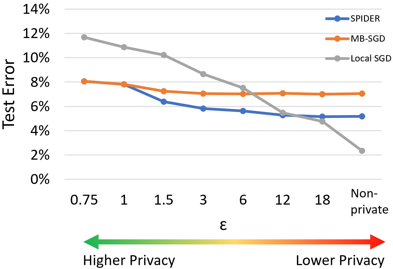
Figure 9: MNIST. $M=12,R=25$.

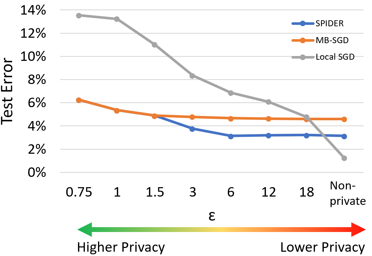
Figure 10: MNIST. $M=25,R=50$.

H.3 CIFAR10 experiment

We run an experiment on CIFAR10 data to further evaluate the performance of ISRL-DP SPIDER in image classification. We partition the data set into 10 heterogeneous silos, each containing one class out of 10 classes of data. We use a 5-layer CNN with two 5x5 convolutional layers (the first with 6 channels, the second with 16 channels, each followed by a ReLu activation and a 2x2 max pooling) and three fully connected layers with 120, 84, 10 neurons in each fully connected layer (the first and second fully connected layers followed by a ReLu activation). For 7 privacy levels ranging from $\epsilon=0.75$ to $\epsilon=18$, we compare ISRL-DP SPIDER against standard FL baselines: MB-SGD, Local SGD (a.k.a. Federated Averaging) ((McMahan et al., 2017)), ISRL-DP MB-SGD ((Lowy and Razaviyayn, 2021b)), and ISRL-DP Local SGD. We fix $\delta=1/n^{2}$. As Figure 6 shows, ISRL-DP SPIDER outperforms both ISRL-DP baselines for most tested privacy levels. The results are based on the average error of 10 random assignment of train/test split of data for each algorithm/epsilon pair. CIFAR10 data is available at https://www.cs.toronto.edu/~kriz/cifar.html. In our implementation, we directly download the data from torchvision.datasets.CIFAR10.

Experimental setup: To divide the CIFAR10 data into $N=10$ heterogeneous silos, we use labels. That is, we assign one unique image class to each of 10 heterogeneous silos.

Preprocessing: We standardize the numerical data to have mean zero and unit variance. We utilize a 80/20 train/test split for data of each client.

Gradient clipping: Since the Lipschitz parameter of the loss is unknown for this problem, we incorporated gradient clipping ((Abadi et al., 2016)) into the algorithms. Noise was calibrated to the clip threshold $L$ to guarantee ISRL-DP (see below for more details). We also allowed the non-private algorithms to employ clipping if it was beneficial.

Hyperparameter tuning: It is similar to hyperparameter tuning of MNIST data. However, we check $(M,R)=(10,50)$ and $(M,R)=(10,100)$ here. Also, the stepsize grid of Local SGD consists of 20 evenly spaced points between $e^{-5}$ and $e^{1}$ for local SGD. The stepsize grid of MB-SGD and SPIDER with R=50 consists of 12 evenly spaced points between $e^{-5}$ and $e^{0}$ and with R=100 consists of 8 evenly spaced points between $e^{-5}$ and $e^{1}$. The clipping threshold of all algorithms includes 6 values of 0.001, 0.01, 0.1, 1, 5, 10. For ISRL-DP FedProx-SPIDER, we use $q\in\{1,2,3,4\}$ for $R=50$ and $q\in\{1,2,\dots,8\}$ for $R=100$. Due to memory limitation, we did not check large $q$ values because it results in large batch size based on $K$ in ISRL-DP FedProx-SPIDER (see below for more details).

Choice of $\sigma^{2}$ and $K$: Same as in MNIST: see Section H.2.

H.4 Breast cancer experiment

We run an experiment on Wisconsin Breast Cancer (Diagnosis) data (WBCD) to further evaluate the performance of ISRL-DP SPIDER in binary (malignant vs. benign) classification. We partition the data set into 2 heterogeneous silos, one containing malignant labels and the other benign labels. We use a 2-layer perceptron with 5 neurons in the hidden layer. For 7 privacy levels ranging from $\epsilon=0.75$ to $\epsilon=18$, we compare ISRL-DP SPIDER against standard FL baselines: MB-SGD, Local SGD (a.k.a. Federated Averaging) ((McMahan et al., 2017)), ISRL-DP MB-SGD ((Lowy and Razaviyayn, 2021b)), and ISRL-DP Local SGD. We fix $\delta=1/n^{2}$. As Figure 8 shows, ISRL-DP SPIDER outperforms both ISRL-DP baselines for most tested privacy levels. The results are based on the average error of 10 random assignment of train/test split of data for each algorithm/epsilon pair. WBCD data is available at https://archive.ics.uci.edu/ml/datasets and we directly download the data from UCI repository website. The experiment is conducted on a device with 6-core Intel Core i7-8700.

Experimental setup: To divide the WBCD data into $N=2$ silos, we use labels (malignant vs. benign). We split the data into 2 parts, one only has malignant labels and the other only has benign data. Then, we assign each part to a client to have full heterogeneous silos. In all experiments, we fix $\delta=1/n^{2}$ (where $n=$number of training samples per client, is given in “Preprocessing”) and test $\epsilon\in\{0.75,1,1.5,3,6,12,18\}$.

Preprocessing: We standardize the numerical data to have mean zero and unit variance. We utilize a 80/20 train/test split for data of each client.

Gradient clipping: Since the Lipschitz parameter of the loss is unknown for this problem, we incorporated gradient clipping ((Abadi et al., 2016)) into the algorithms. Noise was calibrated to the clip threshold $L$ to guarantee ISRL-DP (see below for more details). We also allowed the non-private algorithms to employ clipping if it was beneficial.

Hyperparameter tuning: It is similar to hyperparameter tuning of MNIST data. However, we check $(M,R)=(4,25)$ here. Also, the stepsize grid consists of 15 evenly spaced points between $e^{-9}$ and 1. The clipping threshold includes 4 values of 0.1, 1, 5, 10. For ISRL-DP FedProx-SPIDER, we use $q\in\{1,2,\dots,10\}$. Due to memory limitation, we did not check large $q$ values because it results in large batch size based on $K$ in ISRL-DP FedProx-SPIDER (see below for more details).

Choice of $\sigma^{2}$ and $K$: Same as in MNIST: see Section H.2.

Generating Noise: Due to the low speed of NumPy package in generating multivariate random normal vectors, we use an alternative approach to generate noises. For ISRL-DP SPIDER and ISRL-DP MB-SGD algorithms, we generate the noises on MATLAB and use them in Python when we run the algorithms. Since the number of required noise vectors for ISRL-DP Local SGD is much larger ($K$ times larger) than two other ISRL-DP algorithms, saving the noises beforehand requires a lot of memory. Hence, we generate the noises of ISRL-DP Local SGD on Python by importing a MATLAB engine.

Appendix I Limitations

A major focus of this work is on developing DP algorithms that can handle a broader, more practical range of ML/optimization problems: e.g. non-convex/non-smooth, Proximal-PL, heterogeneous silos. However, some assumptions may still be strict for certain practical applications. In particular, the requirement of an a priori bound on the Lipschitz parameter of the loss–which the vast majority of works on DP ERM and SO also rely on–may be unrealistic in cases where the underlying data distribution is unbounded and heavy-tailed. Understanding what privacy and utility guarantees are possible without this assumption is an interesting problem for future work.

Limitations of Experiments: Pre-processing and hyperparameter tuning were done non-privately, since the focus of this work is on DP FL. This means that the total privacy loss of the entire experimental process is higher than the $\epsilon$ indicated, which only accounts for the privacy loss from executing the FL algorithms with given (fixed) hyperparameters and (pre-processed) data.

Appendix J Societal Impacts

We expect a net positive impact on society from our work, given that our algorithms can prevent sensitive data leakage during FL. Nonetheless, like all technologies, it carries potential for misuse and unintended outcomes. For instance, companies may attempt to legitimize invasive data collection by arguing that the user data will solely be utilized to train a differentially private model to safeguard privacy. Furthermore, in some parameter ranges, privacy comes at the expense of lower model accuracy, which could have adverse effects in crucial applications such as medicine and environmental science.

References

• Abadi et al. (2016) M. Abadi, A. Chu, I. Goodfellow, H. B. McMahan, I. Mironov, K. Talwar, and L. Zhang. Deep learning with differential privacy. Proceedings of the 2016 ACM SIGSAC Conference on Computer and Communications Security, Oct 2016. doi: 10.1145/2976749.2978318. URL http://dx.doi.org/10.1145/2976749.2978318.
• Agarwal et al. (2012) A. Agarwal, P. L. Bartlett, P. Ravikumar, and M. J. Wainwright. Information-theoretic lower bounds on the oracle complexity of stochastic convex optimization. IEEE Transactions on Information Theory, 58(5):3235–3249, 2012. doi: 10.1109/TIT.2011.2182178.
• Arachchige et al. (2019) P. C. M. Arachchige, P. Bertok, I. Khalil, D. Liu, S. Camtepe, and M. Atiquzzaman. Local differential privacy for deep learning. IEEE Internet of Things Journal, 7(7):5827–5842, 2019.
• Arjevani et al. (2019) Y. Arjevani, Y. Carmon, J. C. Duchi, D. J. Foster, N. Srebro, and B. Woodworth. Lower bounds for non-convex stochastic optimization. arXiv preprint arXiv:1912.02365, 2019.
• Arora et al. (2022) R. Arora, R. Bassily, T. González, C. Guzmán, M. Menart, and E. Ullah. Faster rates of convergence to stationary points in differentially private optimization. arXiv preprint arXiv:2206.00846, 2022.
• Bassily et al. (2014) R. Bassily, A. Smith, and A. Thakurta. Private empirical risk minimization: Efficient algorithms and tight error bounds. In 2014 IEEE 55th Annual Symposium on Foundations of Computer Science, pages 464–473. IEEE, 2014.
• Bassily et al. (2019) R. Bassily, V. Feldman, K. Talwar, and A. Thakurta. Private stochastic convex optimization with optimal rates. In Advances in Neural Information Processing Systems, 2019.
• Bassily et al. (2021) R. Bassily, C. Guzmán, and M. Menart. Differentially private stochastic optimization: New results in convex and non-convex settings. arXiv preprint arXiv:2107.05585, 2021.
• Bittau et al. (2017) A. Bittau, U. Erlingsson, P. Maniatis, I. Mironov, A. Raghunathan, D. Lie, M. Rudominer, U. Kode, J. Tinnes, and B. Seefeld. Prochlo: Strong privacy for analytics in the crowd. In Proceedings of the Symposium on Operating Systems Principles (SOSP), pages 441–459, 2017.
• Bubeck et al. (2015) S. Bubeck et al. Convex optimization: Algorithms and complexity. Foundations and Trends® in Machine Learning, 8(3-4):231–357, 2015.
• Bun and Steinke (2016) M. Bun and T. Steinke. Concentrated differential privacy: Simplifications, extensions, and lower bounds. In Proceedings, Part I, of the 14th International Conference on Theory of Cryptography - Volume 9985, page 635–658, Berlin, Heidelberg, 2016. Springer-Verlag. ISBN 9783662536407. doi: 10.1007/978-3-662-53641-4_24. URL https://doi.org/10.1007/978-3-662-53641-4_24.
• Chaudhuri et al. (2011) K. Chaudhuri, C. Monteleoni, and A. D. Sarwate. Differentially private empirical risk minimization. Journal of Machine Learning Research, 12(3), 2011.
• Cheu et al. (2019) A. Cheu, A. Smith, J. Ullman, D. Zeber, and M. Zhilyaev. Distributed differential privacy via shuffling. In Annual International Conference on the Theory and Applications of Cryptographic Techniques, pages 375–403. Springer, 2019.
• Cheu et al. (2021) A. Cheu, M. Joseph, J. Mao, and B. Peng. Shuffle private stochastic convex optimization. arXiv preprint arXiv:2106.09805, 2021.
• Ding et al. (2021) J. Ding, G. Liang, J. Bi, and M. Pan. Differentially private and communication efficient collaborative learning. In Proceedings of the AAAI Conference on Artificial Intelligence, volume 35, pages 7219–7227, 2021.
• Dobbe et al. (2020) R. Dobbe, Y. Pu, J. Zhu, K. Ramchandran, and C. Tomlin. Customized local differential privacy for multi-agent distributed optimization, 2020.
• Dua and Graff (2017) D. Dua and C. Graff. UCI machine learning repository, 2017. URL http://archive.ics.uci.edu/ml.
• Duchi et al. (2013) J. C. Duchi, M. I. Jordan, and M. J. Wainwright. Local privacy and statistical minimax rates. In 2013 IEEE 54th Annual Symposium on Foundations of Computer Science, pages 429–438, 2013. doi: 10.1109/FOCS.2013.53.
• Dwork and Roth (2014) C. Dwork and A. Roth. The Algorithmic Foundations of Differential Privacy. 2014.
• Dwork and Rothblum (2016) C. Dwork and G. N. Rothblum. Concentrated differential privacy. arXiv preprint arXiv:1603.01887, 2016.
• Dwork et al. (2006) C. Dwork, F. McSherry, K. Nissim, and A. Smith. Calibrating noise to sensitivity in private data analysis. In Theory of cryptography conference, pages 265–284. Springer, 2006.
• Erlingsson et al. (2020a) Ú. Erlingsson, V. Feldman, I. Mironov, A. Raghunathan, S. Song, K. Talwar, and A. Thakurta. Encode, shuffle, analyze privacy revisited: Formalizations and empirical evaluation. arXiv preprint arXiv:2001.03618, 2020a.
• Erlingsson et al. (2020b) U. Erlingsson, V. Feldman, I. Mironov, A. Raghunathan, K. Talwar, and A. Thakurta. Amplification by shuffling: From local to central differential privacy via anonymity, 2020b.
• Fang et al. (2018) C. Fang, C. Li, Z. Lin, and T. Zhang. Near-optimal non-convex optimization via stochastic path integrated differential estimator. Advances in Neural Information Processing Systems, 31:689, 2018.
• Feldman et al. (2020) V. Feldman, A. McMillan, and K. Talwar. Hiding among the clones: A simple and nearly optimal analysis of privacy amplification by shuffling, 2020.
• Foster et al. (2019) D. J. Foster, A. Sekhari, O. Shamir, N. Srebro, K. Sridharan, and B. Woodworth. The complexity of making the gradient small in stochastic convex optimization. In Conference on Learning Theory, pages 1319–1345. PMLR, 2019.
• Fredrikson et al. (2015) M. Fredrikson, S. Jha, and T. Ristenpart. Model inversion attacks that exploit confidence information and basic countermeasures. In Proceedings of the 22nd ACM SIGSAC Conference on Computer and Communications Security, pages 1322–1333, 2015.
• Gade and Vaidya (2018) S. Gade and N. H. Vaidya. Privacy-preserving distributed learning via obfuscated stochastic gradients. In 2018 IEEE Conference on Decision and Control (CDC), pages 184–191. IEEE, 2018.
• Geyer et al. (2017) R. C. Geyer, T. Klein, and M. Nabi. Differentially private federated learning: A client level perspective. CoRR, abs/1712.07557, 2017. URL http://arxiv.org/abs/1712.07557.
• Ghazi et al. (2021a) B. Ghazi, R. Kumar, and P. Manurangsi. User-level private learning via correlated sampling. arXiv preprint arXiv:2110.11208, 2021a.
• Ghazi et al. (2021b) B. Ghazi, R. Kumar, P. Manurangsi, R. Pagh, and A. Sinha. Differentially private aggregation in the shuffle model: Almost central accuracy in almost a single message. In International Conference on Machine Learning, pages 3692–3701. PMLR, 2021b.
• Girgis et al. (2021) A. Girgis, D. Data, S. Diggavi, P. Kairouz, and A. Theertha Suresh. Shuffled model of differential privacy in federated learning. In A. Banerjee and K. Fukumizu, editors, Proceedings of The 24th International Conference on Artificial Intelligence and Statistics, volume 130 of Proceedings of Machine Learning Research, pages 2521–2529. PMLR, 13–15 Apr 2021. URL https://proceedings.mlr.press/v130/girgis21a.html.
• He et al. (2019) Z. He, T. Zhang, and R. B. Lee. Model inversion attacks against collaborative inference. In Proceedings of the 35th Annual Computer Security Applications Conference, pages 148–162, 2019.
• Hu et al. (2021) R. Hu, Y. Guo, and Y. Gong. Concentrated differentially private federated learning with performance analysis. IEEE Open Journal of the Computer Society, 2:276–289, 2021. doi: 10.1109/OJCS.2021.3099108.
• Huang and Gong (2020) Z. Huang and Y. Gong. Differentially private ADMM for convex distributed learning: Improved accuracy via multi-step approximation. arXiv preprint:2005.07890, 2020.
• Huang et al. (2020) Z. Huang, R. Hu, Y. Guo, E. Chan-Tin, and Y. Gong. DP-ADMM: ADMM-based distributed learning with differential privacy. IEEE Transactions on Information Forensics and Security, 15:1002–1012, 2020.
• J Reddi et al. (2016) S. J Reddi, S. Sra, B. Poczos, and A. J. Smola. Proximal stochastic methods for nonsmooth nonconvex finite-sum optimization. Advances in neural information processing systems, 29:1145–1153, 2016.
• Jayaraman and Wang (2018) B. Jayaraman and L. Wang. Distributed learning without distress: Privacy-preserving empirical risk minimization. Advances in Neural Information Processing Systems, 2018.
• Joseph et al. (2019) M. Joseph, J. Mao, S. Neel, and A. Roth. The role of interactivity in local differential privacy. In 2019 IEEE 60th Annual Symposium on Foundations of Computer Science (FOCS), pages 94–105. IEEE, 2019.
• Kairouz et al. (2015) P. Kairouz, S. Oh, and P. Viswanath. The composition theorem for differential privacy, 2015.
• Kairouz et al. (2019) P. Kairouz, H. B. McMahan, B. Avent, A. Bellet, M. Bennis, A. N. Bhagoji, K. Bonawitz, Z. Charles, G. Cormode, R. Cummings, R. G. L. D’Oliveira, S. E. Rouayheb, D. Evans, J. Gardner, Z. Garrett, A. Gascón, B. Ghazi, P. B. Gibbons, M. Gruteser, Z. Harchaoui, C. He, L. He, Z. Huo, B. Hutchinson, J. Hsu, M. Jaggi, T. Javidi, G. Joshi, M. Khodak, J. Konečný, A. Korolova, F. Koushanfar, S. Koyejo, T. Lepoint, Y. Liu, P. Mittal, M. Mohri, R. Nock, A. Özgür, R. Pagh, M. Raykova, H. Qi, D. Ramage, R. Raskar, D. Song, W. Song, S. U. Stich, Z. Sun, A. T. Suresh, F. Tramèr, P. Vepakomma, J. Wang, L. Xiong, Z. Xu, Q. Yang, F. X. Yu, H. Yu, and S. Zhao. Advances and open problems in federated learning. arXiv preprint:1912.04977, 2019.
• Kang et al. (2021) Y. Kang, Y. Liu, B. Niu, and W. Wang. Weighted distributed differential privacy erm: Convex and non-convex. Computers & Security, 106:102275, 2021.
• Karimi et al. (2016) H. Karimi, J. Nutini, and M. Schmidt. Linear convergence of gradient and proximal-gradient methods under the polyak-łojasiewicz condition. In Joint European Conference on Machine Learning and Knowledge Discovery in Databases, pages 795–811. Springer, 2016.
• Karimireddy et al. (2020) S. P. Karimireddy, S. Kale, M. Mohri, S. Reddi, S. Stich, and A. T. Suresh. SCAFFOLD: Stochastic controlled averaging for federated learning. In H. D. III and A. Singh, editors, Proceedings of the 37th International Conference on Machine Learning, volume 119 of Proceedings of Machine Learning Research, pages 5132–5143. PMLR, 13–18 Jul 2020.
• Kasiviswanathan et al. (2011) S. P. Kasiviswanathan, H. K. Lee, K. Nissim, S. Raskhodnikova, and A. Smith. What can we learn privately? SIAM Journal on Computing, 40(3):793–826, 2011.
• Kifer et al. (2012) D. Kifer, A. Smith, and A. Thakurta. Private convex empirical risk minimization and high-dimensional regression. In Conference on Learning Theory, pages 25–1. JMLR Workshop and Conference Proceedings, 2012.
• Koloskova et al. (2020) A. Koloskova, N. Loizou, S. Boreiri, M. Jaggi, and S. Stich. A unified theory of decentralized SGD with changing topology and local updates. In H. D. III and A. Singh, editors, Proceedings of the 37th International Conference on Machine Learning, volume 119 of Proceedings of Machine Learning Research, pages 5381–5393. PMLR, 13–18 Jul 2020.
• Krizhevsky et al. (2009) A. Krizhevsky, G. Hinton, et al. Learning multiple layers of features from tiny images. 2009.
• LeCun and Cortes (2010) Y. LeCun and C. Cortes. MNIST handwritten digit database. 2010. URL http://yann.lecun.com/exdb/mnist/.
• Lei et al. (2017) L. Lei, C. Ju, J. Chen, and M. I. Jordan. Non-convex finite-sum optimization via scsg methods. In Proceedings of the 31st International Conference on Neural Information Processing Systems, pages 2345–2355, 2017.
• Lei and Ying (2021) Y. Lei and Y. Ying. Sharper generalization bounds for learning with gradient-dominated objective functions. In International Conference on Learning Representations, 2021.
• Levy et al. (2021) D. Levy, Z. Sun, K. Amin, S. Kale, A. Kulesza, M. Mohri, and A. T. Suresh. Learning with user-level privacy. arXiv preprint arXiv:2102.11845, 2021.
• Li et al. (2020a) T. Li, A. K. Sahu, M. Zaheer, M. Sanjabi, A. Talwalkar, and V. Smith. Federated optimization in heterogeneous networks. Proceedings of Machine Learning and Systems, 2:429–450, 2020a.
• Li et al. (2020b) X. Li, K. Huang, W. Yang, S. Wang, and Z. Zhang. On the convergence of FedAvg on non-iid data. In 8th International Conference on Learning Representations, ICLR 2020, Addis Ababa, Ethiopia, April 26-30, 2020, 2020b. URL https://openreview.net/forum?id=HJxNAnVtDS.
• Liu et al. (2022a) C. Liu, L. Zhu, and M. Belkin. Loss landscapes and optimization in over-parameterized non-linear systems and neural networks. Applied and Computational Harmonic Analysis, 59:85–116, 2022a.
• Liu and Talwar (2019) J. Liu and K. Talwar. Private selection from private candidates. In Proceedings of the 51st Annual ACM SIGACT Symposium on Theory of Computing, pages 298–309, 2019.
• Liu et al. (2020) R. Liu, Y. Cao, H. Chen, R. Guo, and M. Yoshikawa. Flame: Differentially private federated learning in the shuffle model. In AAAI, 2020.
• Liu et al. (2022b) Z. Liu, S. Hu, Z. S. Wu, and V. Smith. On privacy and personalization in cross-silo federated learning. arXiv preprint arXiv:2206.07902, 2022b.
• Lowy and Razaviyayn (2021a) A. Lowy and M. Razaviyayn. Output perturbation for differentially private convex optimization with improved population loss bounds, runtimes and applications to private adversarial training. arXiv preprint:2102.04704, 2021a.
• Lowy and Razaviyayn (2021b) A. Lowy and M. Razaviyayn. Private federated learning without a trusted server: Optimal algorithms for convex losses, 2021b.
• McMahan et al. (2017) B. McMahan, E. Moore, D. Ramage, S. Hampson, and B. A. y Arcas. Communication-efficient learning of deep networks from decentralized data. In Artificial Intelligence and Statistics, pages 1273–1282. PMLR, 2017.
• McMahan et al. (2018) B. McMahan, D. Ramage, K. Talwar, and L. Zhang. Learning differentially private recurrent language models. In International Conference on Learning Representations (ICLR), 2018. URL https://openreview.net/pdf?id=BJ0hF1Z0b.
• McSherry (2009) F. D. McSherry. Privacy integrated queries: an extensible platform for privacy-preserving data analysis. In Proceedings of the 2009 ACM SIGMOD International Conference on Management of data, pages 19–30, 2009.
• Nemirovskii and Yudin (1983) A. S. Nemirovskii and D. B. Yudin. Problem Complexity and Method Efficiency in Optimization. 1983.
• Noble et al. (2022) M. Noble, A. Bellet, and A. Dieuleveut. Differentially private federated learning on heterogeneous data. In International Conference on Artificial Intelligence and Statistics, pages 10110–10145. PMLR, 2022.
• Papernot and Steinke (2021) N. Papernot and T. Steinke. Hyperparameter tuning with renyi differential privacy, 2021.
• Polyak (1963) B. T. Polyak. Gradient methods for the minimisation of functionals. USSR Computational Mathematics and Mathematical Physics, 3(4):864–878, 1963.
• (68) PyTorch team. Training a classifier. https://pytorch.org/tutorials/beginner/blitz/cifar10_tutorial.html#training-a-classifier.
• Rényi (1961) A. Rényi. On measures of entropy and information. In Proceedings of the Fourth Berkeley Symposium on Mathematical Statistics and Probability, Volume 1: Contributions to the Theory of Statistics, volume 4, pages 547–562. University of California Press, 1961.
• Seif et al. (2020) M. Seif, R. Tandon, and M. Li. Wireless federated learning with local differential privacy. In 2020 IEEE International Symposium on Information Theory (ISIT), pages 2604–2609, 2020. doi: 10.1109/ISIT44484.2020.9174426.
• Song et al. (2020) M. Song, Z. Wang, Z. Zhang, Y. Song, Q. Wang, J. Ren, and H. Qi. Analyzing user-level privacy attack against federated learning. IEEE Journal on Selected Areas in Communications, 38(10):2430–2444, 2020. doi: 10.1109/JSAC.2020.3000372.
• Truex et al. (2019) S. Truex, N. Baracaldo, A. Anwar, T. Steinke, H. Ludwig, R. Zhang, and Y. Zhou. A hybrid approach to privacy-preserving federated learning. In Proceedings of the 12th ACM Workshop on Artificial Intelligence and Security, pages 1–11, 2019.
• Truex et al. (2020) S. Truex, L. Liu, K.-H. Chow, M. E. Gursoy, and W. Wei. LDP-Fed: federated learning with local differential privacy. In Proceedings of the Third ACM International Workshop on Edge Systems, Analytics and Networking, page 61–66. Association for Computing Machinery, 2020. ISBN 9781450371322.
• Ullman (2017) J. Ullman. CS7880: rigorous approaches to data privacy, 2017. URL http://www.ccs.neu.edu/home/jullman/cs7880s17/HW1sol.pdf.
• Wang et al. (2017) D. Wang, M. Ye, and J. Xu. Differentially private empirical risk minimization revisited: Faster and more general. In Proc. 31st Annual Conference on Advances in Neural Information Processing Systems (NIPS 2017), 2017.
• Wang et al. (2019a) L. Wang, B. Jayaraman, D. Evans, and Q. Gu. Efficient privacy-preserving stochastic nonconvex optimization. arXiv preprint arXiv:1910.13659, 2019a.
• Wang et al. (2019b) Z. Wang, K. Ji, Y. Zhou, Y. Liang, and V. Tarokh. Spiderboost and momentum: Faster variance reduction algorithms. Advances in Neural Information Processing Systems, 32, 2019b.
• Wei et al. (2020a) K. Wei, J. Li, M. Ding, C. Ma, H. Su, B. Zhang, and H. V. Poor. User-level privacy-preserving federated learning: Analysis and performance optimization. arXiv preprint:2003.00229, 2020a.
• Wei et al. (2020b) K. Wei, J. Li, M. Ding, C. Ma, H. H. Yang, F. Farokhi, S. Jin, T. Q. Quek, and H. V. Poor. Federated learning with differential privacy: Algorithms and performance analysis. IEEE Transactions on Information Forensics and Security, 15:3454–3469, 2020b.
• Woodworth et al. (2020a) B. Woodworth, K. K. Patel, S. Stich, Z. Dai, B. Bullins, B. Mcmahan, O. Shamir, and N. Srebro. Is local SGD better than minibatch SGD? In International Conference on Machine Learning, pages 10334–10343. PMLR, 2020a.
• Woodworth et al. (2020b) B. E. Woodworth, K. K. Patel, and N. Srebro. Minibatch vs local sgd for heterogeneous distributed learning. In H. Larochelle, M. Ranzato, R. Hadsell, M. F. Balcan, and H. Lin, editors, Advances in Neural Information Processing Systems, volume 33, pages 6281–6292. Curran Associates, Inc., 2020b. URL https://proceedings.neurips.cc/paper/2020/file/45713f6ff2041d3fdfae927b82488db8-Paper.pdf.
• Wu et al. (2019) N. Wu, F. Farokhi, D. Smith, and M. A. Kaafar. The value of collaboration in convex machine learning with differential privacy, 2019.
• Yuan and Ma (2020) H. Yuan and T. Ma. Federated accelerated stochastic gradient descent. In H. Larochelle, M. Ranzato, R. Hadsell, M. F. Balcan, and H. Lin, editors, Advances in Neural Information Processing Systems, volume 33, pages 5332–5344. Curran Associates, Inc., 2020. URL https://proceedings.neurips.cc/paper/2020/file/39d0a8908fbe6c18039ea8227f827023-Paper.pdf.
• Zhang et al. (2017) J. Zhang, K. Zheng, W. Mou, and L. Wang. Efficient private erm for smooth objectives, 2017.
• Zhang et al. (2021) Q. Zhang, J. Ma, J. Lou, and L. Xiong. Private stochastic non-convex optimization with improved utility rates. In Proceedings of the Thirtieth International Joint Conference on Artificial Intelligence (IJCAI-21), 2021.
• Zhang et al. (2020) X. Zhang, M. Hong, S. Dhople, W. Yin, and Y. Liu. Fedpd: A federated learning framework with optimal rates and adaptivity to non-iid data. arXiv preprint arXiv:2005.11418, 2020.
• Zhao et al. (2020) Y. Zhao, J. Zhao, M. Yang, T. Wang, N. Wang, L. Lyu, D. Niyato, and K.-Y. Lam. Local differential privacy based federated learning for internet of things. IEEE Internet of Things Journal, 2020.
• Zhou and Tang (2020) Y. Zhou and S. Tang. Differentially private distributed learning. INFORMS Journal on Computing, 32(3):779–789, 2020.
• Zhu and Han (2020) L. Zhu and S. Han. Deep leakage from gradients. In Federated learning, pages 17–31. Springer, 2020.