Encompassing Tests for Nonparametric Regressions

Abstract

We set up a formal framework to characterize encompassing of nonparametric models through the $L^{2}$ distance. We contrast it to previous literature on the comparison of nonparametric regression models. We then develop testing procedures for the encompassing hypothesis that are fully nonparametric. Our test statistics depend on kernel regression, raising the issue of bandwidth’s choice. We investigate two alternative approaches to obtain a “small bias property” for our test statistics. We show the validity of a wild bootstrap method. We empirically study the use of a data-driven bandwidth and illustrate the attractive features of our tests for small and moderate samples.

Keywords: Encompassing, Nonparametric Regression, Bootstrap, Bias Correction,

Locally Robust Statistic.
JEL Classification: C01, C12, C14

1 Introduction

The encompassing principle was introduced in econometrics by Hendry and Richard (1982), Gourieroux et al. (1983), and Mizon and Richard (1986), and further developed in Gourieroux and Monfort (1995), Florens et al. (1996), and Dhaene et al. (1998) among others. It provides a natural principle for choosing between two competing theories: a new theory must be able to accommodate the results obtained by a concurrent older one. An extensive survey is provided in Bontemps and Mizon (2008).

Our goal is to propose encompassing tests for nonparametric models. Our main steps are (i) to formally define encompassing for nonparametric models, (ii) to develop fully nonparametric encompassing tests, and (iii) to show asymptotic validity of a wild bootstrap method for asymptotic inference. Our first contribution is thus to formally set up a framework to precisely define encompassing for nonparametric regression models. We discuss nonparametric encompassing with respect to previous literature on the comparison of such models, whether nested or non nested, see below for references. We show that encompassing reduces neither to significance of some variables nor to the comparison of the models’ theoretical fit. Hence, the null hypothesis of encompassing cannot generally be tested with existing procedures. Our second contribution is to propose fully nonparametric encompassing tests for regression models. Existing encompassing tests rely on parametric functional forms, except for Bontemps et al. (2008) who propose a test aimed at assessing a consequence of encompassing. The new tests we develop directly test the encompassing hypothesis. They are based on an empirical process estimating a continuum of unconditional moments following the Integrated Conditional Moment (ICM) principle introduced by Bierens (1982). Our third contribution is to develop a wild bootstrap method and to show that it provides asymptotically correct inference.

Our fourth contribution is to propose and investigate two approaches to obtain a “small bias property.” Our test statistic depends on an empirical process involving a first-step nonparametric estimator. The small bias property of a semiparametric estimator is that its bias converges to zero faster than the pointwise and integrated bias of the nonparametric estimator on which it is based. A distinguishing feature is that the resulting statistic is $\sqrt{n}$-consistent even when the nonparametric estimator on which it is based converges at the optimal nonparametric rate. Without this property, using a first-step nonparametric estimator necessitates some undersmoothing, and this complicates practical implementation. Newey et al. (2004) have developed a generic technique based on twicing kernels to obtain semiparametric estimators with small bias. We develop here two alternative methods that yield a small bias property. The first one uses a bias-corrected kernel estimator based on the boosting principle (Di Marzio and Taylor, 2008, Park et al., 2009). The second approach is to make the empirical process of interest locally robust with respect to the nonparametric regression. This has previously been used successfully in semiparametric estimation, see Newey (1990) for an early example, and Chernozhukov et al. (2022) for a general approach. We here adapt the two approaches to our empirical process of interest and we show that these yield a small bias property in the asymptotic expansion of our test statistic. This allows for a larger set of smoothing parameters, so the test is expected to be less sensitive to the bandwidth choice.

Our work is related to the extensive literature on consistent specification testing based on empirical processes, see Bierens and Ploberger (1997), Stinchcombe and White (1998), Xia et al. (2004), Escanciano (2006), Delgado and Stute (2008), Lavergne and Patilea (2008) to mention just a few. The main features of our tests compared to previous work are that (i) our empirical process contains a nonparametric kernel estimator, and (ii) due to the form of the null hypothesis we cannot use a density-weighted process, and we thus need to control for a random denominator. Our nonparametric encompassing tests are also connected to the comparison of nonparametric regressions in nested and non nested cases, e.g., Fan and Li (1996), Lavergne and Vuong (1996), Delgado and Manteiga (2001), and Lavergne et al. (2015). We show however that the encompassing hypothesis cannot be tested through existing procedures. Our work is also related to the literature on estimation and testing with nonparametric nuisance components, e.g., Escanciano et al. (2014) and Mammen et al. (2016). The former authors obtain uniform-in-bandwidth expansions for an empirical process similar to the one we consider. We focus here on obtaining a small bias property, but we do not formally establish uniformity in bandwidth.

Our paper is organized as follows. Section 2 formalizes the encompassing notion for nonparametric models and compares our framework to the literature on comparison of nonparametric regressions. Section 3 details the construction of the test statistics and the two approaches used to obtain a small bias property. Section 4 is devoted to the analysis of the asymptotic behavior of our statistics. Since the asymptotic distribution under the null depends on unknown features of the DGP, we establish in Section 5 the validity of a wild bootstrap procedure. Section 6 provides evidence about the small sample performances of our procedures. We check that bootstrapping allows to correctly control size and that our tests have good power. We evaluate the benefits of our bias-reducing approaches, and we investigate thoroughly the influence of the bandwidth as well as of the trimming parameter, which is theoretically necessary. We also provide an empirical illustration. Section 8 contains the proofs of our main results. A supplementary material contains the proof of a technical lemma.

2 Encompassing for Nonparametric Regressions

The definition of encompassing starts with the definition of the binding function, see Gourieroux and Monfort (1995). In a parametric context, we typically start with two competing parameterized families of densities for $Y$, ${\mathcal{M}_{1}}=\{g_{1}(\cdot,\alpha_{1})\,:\,\alpha_{1}\in A_{1}\}$ and ${\mathcal{M}_{2}}:=\{g_{2}(\cdot,\alpha_{2})\,:\,\alpha_{2}\in A_{2}\}$. The pseudo true value of $\alpha_{i}$, $i=1$ or $2$, is defined as

$$\alpha_{i}^{*}=\arg\min_{\alpha_{i}\in A_{i}}d(f(\cdot),g_{i}(\cdot,\alpha_{i}))\,,$$

where $f(\cdot)$ is the true density of $Y$ and $d$ is some divergence between the two distributions, for instance the Kullback-Leibler divergence $\operatorname{E}_{f}\left[\log\left(f(\cdot)/g(\cdot,\alpha)\right)\right]$, with expectation taken with respect to $f(\cdot)$. The binding function $b(\alpha_{1})$ is a correspondence between an element of model ${\mathcal{M}_{1}}$ and the element of model ${\mathcal{M}}_{2}$ that is closest to it. Specifically,

$$b(\alpha_{1})=\arg\min_{\alpha_{2}\in A_{2}}d(g_{1}(\cdot,\alpha_{1}),g_{2}(\cdot,\alpha_{2}))\,.$$

We then say that ${\mathcal{M}_{1}}$ encompasses model ${\mathcal{M}_{2}}$ if $\alpha_{2}^{*}=b(\alpha_{1}^{*})$. That is, ${\mathcal{M}_{1}}$ encompasses ${\mathcal{M}_{2}}$ if the pseudo-true value of the latter can be obtained from the pseudo-true value of the former.

Here we focus on two nonparametric competing models to explain $Y$, where Model $\mathcal{M}_{W}$ uses covariates $W$ and Model $\mathcal{M}_{X}$ uses $X$. A nonparametric model with a specific set of covariates is a function of these variables. To define the pseudo-true value that corresponds to the best explanation of $Y$, we consider the ${L}^{2}$ distance. That is, $\mathcal{M}_{W}$ and $\mathcal{M}_{X}$ are respectively defined as ${L}^{2}(W)$, the space of the square integrable functions of $W$, and ${L}^{2}(X)$. The “pseudo-true functions” are then the regression functions

$$m(W) =\arg\min_{g\in{L}^{2}(W)}\operatorname{E}\left(Y-g(W)\right)^{2}=\operatorname{E}(Y|W),$$

$$\mbox{and }m_{X}(X) =\arg\min_{h\in{L}^{2}(X)}\operatorname{E}\left(Y-h(X)\right)^{2}=\operatorname{E}(Y|X)\,.$$ (1)

The binding function is similarly defined as

$$b(g(W))=\arg\min_{h\in{L}^{2}(X)}\operatorname{E}\left(g(W)-h(X)\right)^{2}=\operatorname{E}\left(g(W)|X\right)\,.$$

We thus say that ${\mathcal{M}_{W}}$ encompasses model ${\mathcal{M}_{X}}$ if

$$b(m(W))=m_{X}(X)\mbox{ a.s.}\Leftrightarrow\operatorname{E}\left(\operatorname{E}(Y|W)|X\right)=\operatorname{E}(Y|X)\mbox{ a.s.}$$ (2)

That is, the regression function of $Y$ on $X$ can be obtained from the regression function of $Y$ on $W$. Similarly, ${\mathcal{M}_{X}}$ encompasses model ${\mathcal{M}_{W}}$ if $\operatorname{E}\left(\operatorname{E}(Y|X)|W\right)=\operatorname{E}(Y|W)$ almost surely.

In what follows, we explore the implications of the definition of nonparametric encompassing and relate it to previous work on the comparison of regression models. In particular, we show that encompassing reduces neither to significance of some variables nor to the comparison of the models’ theoretical fit. Hence, the null hypothesis of encompassing cannot generally be tested with existing procedures.

2.1 Encompassing and Model Fit

Lavergne and Vuong (1996) proposed comparing nonparametric regression models on the basis of their theoretical fit and considered the hypotheses

$$H_{0}\,:\, \operatorname{E}\left[Y-m(W)\right]^{2}-\operatorname{E}\left[Y-m_{X}(X)\right]^{2}=0\,,$$

$$H_{W}\,:\, \operatorname{E}\left[Y-m(W)\right]^{2}-\operatorname{E}\left[Y-m_{X}(X)\right]^{2}<0\,,$$

$$H_{X}\,:\, \operatorname{E}\left[Y-m(W)\right]^{2}-\operatorname{E}\left[Y-m_{X}(X)\right]^{2}>0\,.$$

Non rejection of the null hypothesis $H_{0}$ means that both models have the same theoretical fit. Rejection of $H_{0}$ in favor of either $H_{W}$ or $H_{X}$ indicates which model dominates the other. This framework is quite general since it does not make a distinction between nested and non nested situations and treats the two competing models symmetrically. Lavergne and Vuong (1996) built a test of $H_{0}$ against $H_{W}$ and $H_{X}$ based on the comparison of the empirical analogs of the models’ fit.

Comparing nonparametric regressions through their fit seems natural. Does encompassing imply a better fit for the encompassing model? As we detail below, the answer is yes: if $\mathcal{M}_{W}$ encompasses $\mathcal{M}_{X}$, the theoretical fit of $\operatorname{E}(Y|W)$ is at least as good as the one of $\operatorname{E}(Y|X)$, and is strictly better except when $\operatorname{E}(Y|W)=\operatorname{E}(Y|X)\mbox{ a.s.}$

Proposition 2.1.

If $\mathcal{M}_{W}$ encompasses $\mathcal{M}_{X}$,

1. $H_{X}$ cannot hold,

2. $H_{0}$ holds iff $\operatorname{E}(Y|W)=\operatorname{E}(Y|X)\mbox{ a.s.}$ iff $\mathcal{M}_{X}$ encompasses $\mathcal{M}_{W}$.

Proof.

Consider Statement (a). Since $\operatorname{E}(\operatorname{E}(Y|W)|X)=\operatorname{E}(Y|X)\mbox{ a.s.}$,

$$E\left[Y-\operatorname{E}(Y|X)\right]^{2} =\operatorname{E}\left[Y-\operatorname{E}(Y|W)\right]^{2}+\operatorname{E}\left[\operatorname{E}(Y|W)-\operatorname{E}(Y|X)\right]^{2}\,,$$

as the cross-term cancels, and $E\left[Y-\operatorname{E}(Y|X)\right]^{2}\geq\operatorname{E}\left[Y-\operatorname{E}(Y|W)\right]^{2}$.

Consider Statement (b). It is obvious that if $\operatorname{E}(Y|W)=\operatorname{E}(Y|X)\mbox{ a.s.}$ then $H_{0}$ holds and both models encompass each other. By Lavergne and Vuong (1996, Lemma 1), if one model encompasses the other and $H_{0}$ holds, it should be that $\operatorname{E}(Y|W)=\operatorname{E}(Y|X)$. Finally, if both models encompass each other, then $H_{0}$ holds by Statement (a). ∎

Therefore, except in the case where the two regressions are equal, encompassing implies a strictly better fit for the encompassing model. Conversely, one model can have a better fit than another without encompassing it, see Lavergne and Vuong (1996) for some examples where this happens. Hence, the encompassing concept is not tailored for model selection.

The test statistic proposed by Lavergne and Vuong (1996) to compare models’ fit is asymptotically degenerate under $H_{0}$ when the two models are “generalized nested regressions,” that is when either $\operatorname{E}(\operatorname{E}(Y|W)|X)=\operatorname{E}(Y|X)\mbox{ a.s.}$ or $\operatorname{E}(\operatorname{E}(Y|X)|W)=\operatorname{E}(Y|W)\mbox{ a.s.}$ Hence their test cannot be used when there is encompassing, and the tests we develop below are complementary to theirs. The latter might also be used as preliminary tests to check whether their test can be entertained. This would imply (i) testing whether Model ${\cal M}_{X}$ encompasses Model ${\cal M}_{W}$, and (ii) testing whether Model ${\cal M}_{W}$ encompasses Model ${\cal M}_{X}$. One rejection among two would imply (we cannot reject) that the encompassing model has a strictly better fit than the encompassed one; no rejection would mean (we cannot reject) that $\operatorname{E}(Y|W)=\operatorname{E}(Y|X)\mbox{ a.s.}$ Only if we rejected twice would we need to entertain the test of Lavergne and Vuong (1996) to determine whether one model has a better fit. A more direct alternative to this involved procedure is to apply the test proposed by Liao and Shi (2020), which is universally valid. We leave the study of the respective merits of these competing procedures for future work.

2.2 Encompassing and Significance

When the two sets of regressors are nested, specifically when $W=(X,Z)$, then it is clear that (2) holds. A more interesting question is whether ${\mathcal{M}_{X}}$ encompasses ${\mathcal{M}_{W}}$, that is whether

$$\operatorname{E}\left(\operatorname{E}(Y|X)|X,Z\right)=\operatorname{E}(Y|X)=\operatorname{E}(Y|X,Z)\mbox{ a.s.}$$

In this setup, encompassing is equivalent to whether $Z$ is significant in the regression function of $Y$ on $X$ and $Z$. Significance testing in nonparametric regressions has been a focus of extensive work, see Fan and Li (1996), Lavergne and Vuong (2000), Ait-Sahalia et al. (2001), Lavergne (2001), Delgado and Manteiga (2001).

Consider now two nonnested sets of regressors, and assume the regressors $X$ are not significant once we control for $W$, that is

$$\operatorname{E}(Y|W,X)=\operatorname{E}(Y|W)\mbox{ a.s.}$$ (3)

By conditioning again with respect to $X$, one obtains that

$$\operatorname{E}(Y|X)=\operatorname{E}[\operatorname{E}(Y|W)|X]\mbox{ a.s.}$$

so that $\mathcal{M}_{W}$ encompasses $\mathcal{M}_{X}$. Bontemps et al. (2008) consider (3) as their hypothesis of interest, since it implies encompassing. The other direction of the implication, however, does not hold: if $\mathcal{M}_{W}$ encompasses $\mathcal{M}_{X}$, then it is not necessarily true that the covariates $X$ are not significant in the nonparametric regression of $Y$ onto $(W,X)$, as shown below.

Proposition 2.2.

$\mathcal{M}_{W}$ encompasses $\mathcal{M}_{X}$ if and only if

$$\operatorname{E}\left(Y|W,X\right)=\operatorname{E}(Y|W)+g(W,X)\qquad\mbox{with }\,\operatorname{E}\left[g(W,X)|W\right]=\operatorname{E}\left[g(W,X)|X\right]=0\mbox{ a.s.}$$

Proof.

By definition, $Y=\operatorname{E}(Y|W)+\varepsilon$ with $\operatorname{E}(\varepsilon|W)=0$. Hence,

$$\operatorname{E}(Y|W,X)=\operatorname{E}(Y|W)+\operatorname{E}(\varepsilon|W,X)=\operatorname{E}(Y|W)+g(W,X)\,.$$

Conditioning on $W$ yields $\operatorname{E}\left[g(W,X)|W\right]=0$. Conditioning on $X$ and using the fact that $\mathcal{M}_{W}$ encompasses $\mathcal{M}_{X}$ yields $\operatorname{E}\left[g(W,X)|X\right]=0$. This shows necessity. Sufficiency similarly follows by conditioning $\operatorname{E}\left(Y|W,X\right)=\operatorname{E}(Y|W)+g(W,X)$ on $X$ and using $\operatorname{E}\left[g(W,X)|X\right]=0$. ∎

The previous result highlights that for non nested sets of regressors, the encompassing property does not reduce to the significance of some regressors in the complete regression. As long as $g(W,X)$ is not a.s. equal to zero, $\mathcal{M}_{W}$ encompasses $\mathcal{M}_{X}$, but $X$ is a significant covariate in $\operatorname{E}(Y|W,X)$. The following provides a concrete example.

Example.

Let $W$ be continuous univariate, symmetrically distributed around 0, with density $f_{W}(\cdot)$. Consider $p(\cdot)\in(0,1)$, $\varphi(\cdot)$ and $\psi(\cdot)$ two univariate densities with mean 0. Define

$$f_{X|W}(x|w)=p(w)\varphi(x)+(1-p(w))\psi(x)\,,$$

so that $X$ has a mixture distribution conditionally on $W$. Then

$$f_{X}(x) =\left[\int p(w)f_{W}(w)\,dw\right]\varphi(x)+\left[\int(1-p(w))f_{W}(w)\,dw\right]\psi(x)\,,$$

$$f_{W|X}(w|x) =\frac{f_{W}(w)}{f_{X}(x)}\left(p(w)\varphi(x)+(1-p(w))\psi(x)\right)\,.$$

Let

$$Y=m(W)+h(W)X+\eta\,,\qquad\operatorname{E}(\eta|W,X)=0\,.$$

Then

$$\operatorname{E}(X|W)=p(W)\int{x\varphi(x)\,dx}+(1-p(W))\int{x\psi(x)\,dx}=0\,.$$

One can select $h(\cdot)$ and $p(\cdot)$ so that $\operatorname{E}[h(W)|X]=0$. Consider first a case where $h(\cdot)$ is an odd function with mean 0 and $p(\cdot)$ is even. Then by the symmetry of $f_{W}(\cdot)$, $\operatorname{E}[h(W)|X]=0$. Another setup used in our simulations below is for $h(\cdot)$ even with mean 0 and $p(-w)=1-p(w)$. Again, it is easy to show that $\operatorname{E}[h(W)|X]=0$.

Whenever $\operatorname{E}[h(W)|X]=0$, then $\operatorname{E}[h(W)X|W]=\operatorname{E}[h(W)X|X]=0$, and $\mathcal{M}_{W}$ encompasses $\mathcal{M}_{X}$, but $X$ is significant in $\operatorname{E}(Y|W,X)$. Furthermore, $\mathcal{M}_{X}$ does not encompass $\mathcal{M}_{W}$ in general. If this holds, then $m(W)=\operatorname{E}(Y|X)$ a.s. from Proposition 2.1. Integrating both sides with respect to the marginal density $f_{X}(\cdot)$ implies that $m(W)$ and thus $\operatorname{E}(Y|X)$ are both constant almost surely.

3 Tests Statistics

3.1 ICM Statistic

We want to test

$${H}_{0}\,:\,\operatorname{E}\left(\operatorname{E}(Y|W)|X\right)=\operatorname{E}(Y|X)\mbox{ a.s.}\Leftrightarrow\operatorname{E}\left(Y-\operatorname{E}(Y|W)|X\right)=0\mbox{ a.s.}$$

against its logical complement ${H}_{1}={H}_{0}^{c}$. While $H_{0}$ is a conditional moment restriction, we can consider instead an equivalent continuum of unconditional moments. Assume $X\in\mathbb{R}^{d}$ has bounded support, which is without loss of generality, as we can always transform $X$ by a one-to-one function that maps it to a compact set. Then the null hypothesis is equivalent to

$${H}_{0}\,:\,\operatorname{E}\left[\left(Y-\operatorname{E}(Y|W)\right)\varphi(s^{\prime}X)\right]=0\ \mbox{ a.s.}\quad\forall s\in{\cal S}\,,$$ (4)

where ${\cal S}$ is a (arbitrary) neighborhood of the origin in $\mathbb{R}^{d}$ and $\varphi(\cdot)$ is a well-chosen function, see Assumption A below for precise conditions. Some convenient choices for $\varphi(\cdot)$ are as follows. Bierens (1982) shows the previous equivalence for the complex exponential $\varphi(u)=\exp(iu)$, Bierens (1990) considers the exponential $\varphi(u)=\exp(u)$, Bierens and Ploberger (1997) the logistic c.d.f. $\varphi(u)=1/(1+\exp(c-u))$, see also Stinchcombe and White (1998). Other types of functions could be used such as indicator functions (Escanciano, 2006, Delgado and Manteiga, 2001).

If we observe a random sample $(Y_{i},W_{i},X_{i})$, $i=1,\ldots n$, from $(Y,W,X)$, and if we know the precise form of $\operatorname{E}(Y|W)$, then Bierens’ Integrated Conditional Moment (ICM) statistic for testing $H_{0}$ is

$$\int_{\mathbb{R}^{d}}{\left|n^{-1/2}\sum_{j=1}^{n}{\left(Y_{j}-{\operatorname{E}}(Y|W_{j})\right)\varphi(s^{\prime}X_{j})}\right|^{2}\,d\mu(s)}\,,$$ (5)

where $\mu$ is some probability measure on ${\cal S}$, such as the uniform distribution on ${\cal S}$. Alternatively, a Kolmogorov-Smirnov type statistic could be considered, but the Cramer-von-Mises form appears to be easier to deal with in practice, see below.

In practice, we use a kernel nonparametric estimator of the conditional expectation $\operatorname{E}(Y|W)$. Let $K(\cdot)$ be a kernel on $\mathbb{R}^{p}$, $h\,(=h_{n})$ a bandwidth, and $K_{{h}}(u)=K\left(u_{1}/h,\ldots u_{p}/h\right)$. Define

$$\overline{Y}(w)=\left(nh^{p}\right)^{-1}\sum_{i=1}^{n}Y_{i}K_{h}\left({W_{i}-w}\right)\,.$$

With $e=(1,\ldots,1)^{\prime}$, let $\widehat{f}(w)=\overline{e}(w)$, and $\widehat{m}(w)=\overline{Y}(w)/\widehat{f}(w)$.

To control for the random denominator in the kernel estimator, we introduce a trimming factor $\widehat{t}(w)=\mathbf{1}\left(\widehat{f}(w)\geq\tau_{n}\right)$, where $\tau_{n}$ converges to zero. Let $\widehat{\varepsilon}_{i}=Y_{i}-\widehat{m}(W_{i})$, $\phi_{s}(\cdot)=\varphi(s^{\prime}\cdot)$, and $\mathbb{P}_{n}(g)=n^{-1}\sum_{i=1}^{n}g(Z_{i})$ denote the empirical mean process based on $g(\cdot)$. An ICM test statistic can be built upon the process $\mathbb{P}_{n}\left(\widehat{\varepsilon}\phi_{s}\widehat{t}\right)$ as

$$S_{n}=n\,\int_{{\cal S}}|\mathbb{P}_{n}\left(\widehat{\varepsilon}\phi_{s}\widehat{t}\right)|^{2}\,d\mu(s)\,.$$

In our practical implementation, we chose $\varphi(\cdot)$ as the complex exponential and $\mu$ to be symmetric around the origin. Define

$$a(z)=\int_{{\cal S}}\exp(is^{\prime}z)\,d\mu(s)=\int_{{\cal T}}\cos(s^{\prime}z)\,d\mu(s)\,,$$

due to the symmetry of $\mu$, and let $\widehat{\bm{\varepsilon}}=\left(\widehat{\varepsilon}_{j},j=1,\ldots n\right)^{\prime}$ and $\widehat{t}_{i}=\widehat{t}(W_{i})$. Then the statistic becomes

$$\int_{{\cal S}}{n^{-1}\sum_{j=1}^{n}\sum_{m=1}^{n}{\widehat{\varepsilon}_{j}\widehat{\varepsilon}_{m}\widehat{t}_{j}\widehat{t}_{m}\exp(is^{\prime}(X_{j}-X_{m}))}\,d\mu(s)}$$

$$=n^{-1}\sum_{j=1}^{n}\sum_{m=1}^{n}{\widehat{\varepsilon}_{j}\widehat{\varepsilon}_{m}\widehat{t}_{j}\widehat{t}_{m}\int_{{\cal S}}{\cos(s^{\prime}(X_{j}-X_{m}))}\,d\mu(s)}=\widehat{\bm{\varepsilon}}^{\prime}\bm{A}\widehat{\bm{\varepsilon}}\,,$$

where $\bm{A}$ is a matrix with generic element $n^{-1}a\left(X_{j}-X_{m}\right)\widehat{t}_{j}\widehat{t}_{m}$. In practice the function $a(\cdot)$ is the Fourier transform of $\mu$, so we can choose the latter so that the former has an analytic expression, and computation of the matrix $A$ is fast. To achieve scale invariance, we recommend, as in Bierens (1982), to scale each component of $X$ by a measure of dispersion, such as the empirical standard deviation.

The behavior of $\sqrt{n}\mathbb{P}_{n}\left(\widehat{\varepsilon}\phi_{s}\widehat{t}\right)$ is studied in detail by Escanciano et al. (2014), who derived a uniform expansion. Hence, the properties of the ICM test based on $S_{n}$ can be derived from their results. However, these impose undersmoothing in kernel estimation, which ensures that the bias disappears fast enough, but makes the practical bandwidth choice tricky. In what follows, we develop two approaches to avoid undersmoothing, and in particular to allow for an optimal nonparametric bandwidth. This is convenient because there are well-known methods for approximating such bandwidths.

3.2 Bias Corrected Estimation

Newey et al. (2004) obtained a small bias property for density weighted average semiparametric estimators. Here we instead rely on an idea developed in the boosting literature for kernel regressions (Di Marzio and Taylor, 2008, Park et al., 2009). Xia et al. (2004) used a similar bias correction in a specification test for a single-index model.

$L^{2}$ boosting starts with an initial nonparametric estimator and builds a bias-corrected updated estimator. The bias correction is roughly based on nonparametric residuals. The method can be iterated, but we will restrict to a single boosting step, which is sufficient for our purpose. In our context, the bias correction to be applied to $\widehat{m}(w)$ is

$$\widehat{B}(w)=\frac{\overline{\widehat{m}}(w)}{\widehat{f}(w)}-\widehat{m}(w)\,,$$

where

$$\overline{\widehat{m}}(w)=(nh^{p})^{-1}\sum_{i=1}^{n}\widehat{m}(W_{i})\widehat{t}_{i}K_{h}(W_{i}-w)\,,$$ (6)

and the trimming controls for the random denominator of $\widehat{m}$. The bias-corrected estimator thus is

$$\widetilde{m}(w)=\widehat{m}(w)-\widehat{B}(w)=2\widehat{m}(w)-\frac{\overline{\widehat{m}}(w)}{\widehat{f}(w)}\,.$$ (7)

We then consider $\widetilde{\varepsilon}_{i}=Y_{i}-\widetilde{m}(W_{i})$ and the bias-corrected ICM statistic

$$S_{n}^{BC}=n\,\int_{{\cal S}}|\mathbb{P}_{n}\left(\widetilde{\varepsilon}\phi_{s}\widehat{t}\right)|^{2}\,d\mu(s)\,.$$

The form (7) of our bias corrected estimator is similar to the one discussed in Newey et al. (2004, Section 3) who considered density-weighted nonparametric estimators. To use their technique in our setup would necessitate applying their correction to both the numerator and the denominator of the regression estimator. We feel more natural and practically more convenient to correct for the bias of the regression estimator as described above.

3.3 Locally Robust Process

Locally robust semiparametric estimation has been considered by several authors, see Newey (1990) for an early example. Chernozhukov et al. (2022) consider a general GMM estimation problem, where the moments depend on a first-step nonparametric estimator. Locally robust semiparametric GMM estimators are built from moment conditions that have zero derivatives with respect to the first-step estimator so that the latter does not affect the asymptotic variance of the parameters of interest. They have smaller bias and better small sample properties than standard GMM estimators.

In our case, we have a continuum of moment conditions. Our goal is to modify these moment conditions so that (i) we can still test for our null hypothesis of interest using these modified moments, and (ii) estimation becomes “adaptive” with respect to the nonparametric regression. Hence, we consider the moments

$$\operatorname{E}\left[\left(Y-\operatorname{E}(Y|W)\right)\left(\varphi(s^{\prime}X)-\operatorname{E}(\varphi(s^{\prime}X)|W)\right)\right]=0\ \quad\forall s\in{\cal S}\,.$$

Because for any $s$, $\operatorname{E}\left[\left(Y-\operatorname{E}(Y|W)\right)\operatorname{E}(\varphi(s^{\prime}X)|W)\right]=0$, the above moment conditions are equivalent to (4). We show below that for the empirical equivalent of these moments, estimation of nonparametric components has no first order effect.

Let $\iota_{s}(W)=\operatorname{E}(\phi_{s}(X)|W)$ and its estimator

$$\widehat{\iota}_{s}(w)=\overline{\phi_{s}}(w)/\widehat{f}(w)\,,\qquad\overline{\phi_{s}}(w)=\left(nh^{p}\right)^{-1}\sum_{i=1}^{n}\phi_{s}(X_{i})K_{h}\left({W_{i}-w}\right)\,.$$

Our locally robust approach thus delivers the statistic

$$S_{n}^{LR}=n\,\int_{{\cal S}}|\mathbb{P}_{n}\left(\widehat{\varepsilon}(\phi_{s}-\widehat{\iota}_{s})\widehat{t}\right)|^{2}\,d\mu(s)\,.$$

Newey et al. (2004) note that their bias correction based on twicing kernels is equivalent to a locally robust density weighted average. By contrast, our bias correction detailed in the previous section does not yield the same statistic as the one based on the locally robust process. In practice, there is no need to compute $\widehat{\iota}_{s}(W)$ for each $s\in{\cal S}$ and to integrate. Simple algebra reveals that, if $\bm{K}$ denotes the $n\times n$ matrix of generic element $K_{h}(W_{i}-W_{j})/[nh^{p}\widehat{f}(W_{j})]$, then

$$S_{n}^{LR}=\widehat{\bm{\varepsilon}}^{\prime}\bm{A}\widehat{\bm{\varepsilon}}-2\widehat{\bm{\varepsilon}}^{\prime}\bm{A}\bm{K}\widehat{\bm{\varepsilon}}+\widehat{\bm{\varepsilon}}^{\prime}\bm{K}^{\prime}\bm{A}\bm{K}\widehat{\bm{\varepsilon}}\,,$$

so the locally robust version of the statistic is practically straightforward to compute.

4 Asymptotic Analysis

We here focus on the asymptotic expansion of the empirical processes on which our test statistics $S_{n}^{BC}$ and $S_{n}^{LR}$ are based. We do not formally consider the empirical process entering $S_{n}$: its properties would be similar but would necessitate assuming some undersmoothing.

We first introduce some definitions. Define the differential operator

$$\partial^{l}g(w)=\frac{\partial^{|l|}}{\partial^{l_{1}}w_{1}\ldots\partial^{l_{p}}w_{p}}g(w)\qquad l=(l_{1},..,l_{p})^{\prime},\ |l|=l_{1}+..+l_{p}\,.$$

Definition 4.1.

(a) $\mathcal{G}_{\lambda}(\mathcal{A})=\left\{g:\mathcal{A}\mapsto\mathbb{R}:\quad\sup_{a\in\mathcal{A}}|\partial^{l}g(a)|<M\text{ for all }|l|\leq\lambda\right\}$. (b) $\mathcal{K}_{\lambda}^{r}$ is the class of product univariate kernels $k(\cdot)$ such that $k(\cdot)$ is of order $r$, $\lambda$ times continuously differentiable with uniformly bounded derivatives, symmetric about zero, and with bounded support.

Assumption A.

(i) $(Y_{i},W_{i},X_{i}),i=1,\ldots n$, is a random sample from $(Y,W,X)$. $\mathcal{Y}\subset\mathbb{R}$, ${\cal W}\subset\mathbb{R}^{p}$, and ${\cal X}\subset\mathbb{R}^{d}$, the supports of $Y$, $W$, and $X$, are bounded. (ii) ${\cal S}$ is a bounded compact subset of $\mathbb{R}^{d}$ containing a neighborhood of the origin. (iii) $\varphi(\cdot)$ is an analytic non polynomial function with $\partial^{l}\varphi(0)\neq 0$ for all $l\in\mathbb{N}$.

Assumption B.

(i) $f(\cdot)\in\mathcal{G}_{r}({\mathbb{R}^{p}})$ and $m(\cdot)\in\mathcal{G}_{r}(\cal W)$, with $r\geq\lceil(p+1)/2\rceil$. (ii) $\iota_{s}(\cdot)\in\mathcal{G}_{r}({\cal W})$ uniformly in $s\in{\cal S}$, with $r\geq\lceil(p+1)/2\rceil$. (iii) $K(\cdot)\in\mathcal{K}_{\lambda}^{r}$ with $\lambda\geq\lceil(p+1)/2\rceil$.

Define the uniform convergence rate of the kernel density estimator as

$$d_{n} =\sqrt{\frac{\log n}{nh_{n}^{p}}}+h_{n}^{r}\,.$$

Assumption C.

(i) $h_{n}\tau_{n}^{-1}=o(1)$. (ii) $d_{n}\tau_{n}^{-3}=o(n^{-1/4})$. (iii) $d_{n}h^{-|l|}\tau_{n}^{-(2+|l|)}=o(1)$ for $|l|=\lceil(p+1)/2\rceil$.

Assumption D.

(i) $p_{n}=\Pr\left(f(W)\leq 3\tau_{n}/2\right)$ is such that $p_{n}=o(n^{-1/2})$ , $p_{n}h_{n}^{-p}\tau_{n}^{-2}=o(n^{-1/4})$, and $p_{n}h_{n}^{-(p+|l|)}\tau_{n}^{-(1+|l|)}=o(1)$ for $|l|=\lceil(p+1)/2\rceil$.

(ii) There exists $N$ such that for all $n\geq N$, $\mathcal{W}_{n}=\left\{w:f(w)\geq\tau_{n}/2\right\}$ is convex.

Assumption A ensures that the encompassing hypothesis can be written as the continuum of moment conditions (4). In particular, Bierens (2017, Theorem 2.2) builds on previous results by Bierens (1982) and Stinchcombe and White (1998), and shows that A-(iii) is sufficient. Intuitively, if $\varphi(\cdot)$ is analytic non-polynomial, Equation (4) implies that $Y-\operatorname{E}(Y|W)$ is uncorrelated with any polynomial in $s^{\prime}X$, and thus yields the required equivalence. This allows for different functions $\varphi(\cdot)$ as previously detailed.

Assumption B imposes conditions that are commonly found in the literature on nonparametric estimation. In particular, they impose that the density of $W$ is differentiable over $\cal W$ and its derivatives go smoothly to zero as we approach to the boundaries of the support. Part (ii) is necessary only for the study of the locally robust empirical process, which involves a nonparametric estimator of $\iota_{s}(\cdot)$.

Assumption C sets the main conditions on the bandwidths. Together with Assumption B, it implies that the kernel estimators asymptotically belong to a class of sufficiently smooth functions with limited entropy/complexity. This is needed for the asymptotic stochastic equicontinuity of the empirical processes at the basis of our test statistics. Assumptions C and D impose conditions on the bandwidths in connection with the trimming parameter. We need the effect of trimming to vanish quickly enough to avoid large biases. Abstracting from the appearance of the trimming, Condition (ii) in Assumption C ensures that the kernel estimators are $n^{-1/4}$-consistent. It requires in particular that $nh_{n}^{4r}=o(1)$. Without the bias correction or locally robust approach employed in the construction of our statistics, this condition would become $nh_{n}^{2r}=o(1)$ to ensure that the bias of the nonparametric estimator is negligible compared to the variability of the empirical process, see Delgado and Manteiga (2001) or Escanciano et al. (2014). This means that our empirical processes have a small bias property (in their stochastic expansion). Our conditions allow the bandwidth to be optimal for nonparametric estimation purposes and avoid the need for undersmoothing. The main practical advantage is that one can use for instance a simple rule-of-thumb. We could extend our theoretical results to stochastic bandwidths to allow for the use of data-driven methods, as was done in other contexts (Andrews, 1995, Mammen, 1992, Lavergne, 2001). The details would be more involved here because of the stochastic trimming, so we do not pursue this issue further.

Assumption D as a whole is used to ensure that trimming has a negligible effect overall, see e.g. Lavergne and Vuong (1996) or Escanciano et al. (2014) for similar assumptions. It may be difficult to check, but our simulations seem to indicate that trimming is actually not crucial: when a data-driven bandwidth is used, results with no trimming are comparable, and mostly better, than results with trimming.

The following proposition establishes the influence function representations of the empirical processes used in our statistics $S_{n}^{BC}$ and $S_{n}^{LR}$.

Proposition 4.2.

Under Assumptions A–D, $\sqrt{n}\mathbb{P}_{n}(\widetilde{\varepsilon}\phi_{s}\widehat{t})=\sqrt{n}\mathbb{P}_{n}(\varepsilon(\phi_{s}-\iota_{s}))+o_{P}(1)$ and $\sqrt{n}\mathbb{P}_{n}(\widehat{\varepsilon}(\phi_{s}-\widehat{\iota}_{s})\widehat{t})=\sqrt{n}\mathbb{P}_{n}(\varepsilon(\phi_{s}-\iota_{s}))+o_{P}(1)$ uniformly in $s\in{\cal S}$.

From the above result, under $H_{0}$ the limiting distribution, say $\mathbb{G}_{s}$, of both empirical processes is the limiting one of $\sqrt{n}\mathbb{P}_{n}(\varepsilon(\phi_{s}-\iota_{s}))$. This $\mathbb{G}_{s}$ is a zero-mean tight Gaussian process valued in $L^{\infty}(\cal S)$, the space of uniformly bounded functionals over $\cal S$, and characterized by the collection of covariances $\{\operatorname{E}(Y-m(W))^{2}(\phi_{s}(X)-\iota_{s}(X))(\phi_{t}(X)-\iota_{t}(W)):s,t\in\mathcal{S}\}$. Our asymptotic expansions directly yield

$$S_{n}^{BC}\quad\mbox{or }\quad S_{n}^{LR}\ \mbox{$\stackrel{{\scriptstyle d}}{{\longrightarrow}}\,$}\int{\left|\mathbb{G}_{s}\right|^{2}\,d\mu(s)}\,.$$

However, the result is not useful in practice since the covariance function of $\mathbb{G}_{s}$ depends on the unknown data generating process. In what follows, we develop a bootstrap procedure for obtaining critical and p-values.

5 Bootstrap Tests

We use a wild bootstrap procedure that imposes the null hypothesis $H_{0}$ when resampling the observations. The bootstrap data generating process (DGP) writes as

$$Y_{i}^{*} =\widehat{m}(W_{i})+\xi_{i}\widehat{\varepsilon}_{i}\qquad\widehat{\varepsilon}_{i}=Y_{i}-\widehat{m}(W_{i})\,,$$

where $\{\xi_{i},i=1,\ldots n\}$ is a sequence of independent bootstrap weights with $\operatorname{E}\xi=0$ and $\operatorname{E}\xi^{2}=1$. From each bootstrap sample $\{\left(Y_{i}^{*},W_{i},X_{i}\right)\text{ : }i=1,..,n\}$, we proceed as above to obtain $\widehat{\varepsilon}^{*}=Y_{i}^{*}-\widehat{m}^{*}(W_{i})$ and $\widetilde{\varepsilon}_{i}^{*}=Y_{i}^{*}-\widetilde{m}^{*}(W_{i})$, where

$$\widetilde{m}^{*}(w)=\widehat{m}^{*}(w)-\widehat{B}^{*}(w) =\widehat{m}^{*}(w)-\left(\frac{\overline{\widehat{m}^{*}}(w)}{\widehat{f}(w)}-\widehat{m}^{*}(w)\right),\qquad\widehat{m}^{*}=\overline{Y^{*}}/\widehat{f}\,.$$

The kernel smoothers $\overline{Y^{*}}$ and $\overline{\widehat{m}^{*}}$ are constructed in the same way as in Equation (6) to control for the random denominators in $Y^{*}$ and $\widehat{m}^{*}$. The bias correction could be the one used in the original statistic, as done by Xia et al. (2004), however we noted in simulations that recomputing the bias correction with bootstrap data yields a better behavior. We thus consider the bootstrap statistics

$$n\int_{{\cal S}}|\mathbb{P}_{n}\left(\widetilde{\varepsilon}^{*}\phi_{s}\widehat{t}\right)|^{2}\,d\mu(s) \quad\mbox{and }\quad n\int_{{\cal S}}|\mathbb{P}_{n}\left(\widehat{\varepsilon}^{*}(\phi_{s}-\widehat{\iota}_{s})\widehat{t}\right)|^{2}\,d\mu(s)\,.$$ (8)

In practice, one can compute many bootstrap statistics and obtain their $1-\alpha$ quantiles, denoted as ${q}_{1-\alpha}^{BC}$ and ${q}_{1-\alpha}^{LR}$. The bootstrap test rejects $H_{0}$ whenever $S_{n}^{j}>{q}_{1-\alpha}^{j}$, for $j=BC$ or $LR$.

Proposition 5.1.

Let $\{\xi_{i},i=1,\ldots n\}$ be an i.i.d. sequence with $\operatorname{E}\xi=0$, $\operatorname{E}\xi^{2}=1$, and $\operatorname{E}|\xi|^{3}<\infty$ independent of the sample. Under Assumptions A-D,

(a) $\sqrt{n}\mathbb{P}_{n}(\widetilde{\varepsilon}^{*}\phi_{s}\widehat{t})=\sqrt{n}\mathbb{P}_{n}(\xi\varepsilon(\phi_{s}-\iota_{s}))+o_{p}(1)$ and $\sqrt{n}\mathbb{P}_{n}(\widehat{\varepsilon}^{*}(\phi_{s}-\widehat{\iota}_{s})\widehat{t})=\sqrt{n}\mathbb{P}_{n}(\xi\varepsilon(\phi_{s}-\iota_{s}))+o_{p}(1)$ uniformly in $s\in{\cal S}$.

(b) Under $H_{0}$, $\Pr\left[S_{n}^{j}>{q}_{1-\alpha}^{j}\right]\rightarrow\alpha$, $j=BC$ or $LR$.

(c) Under $H_{1}$, $\Pr\left[S_{n}^{j}>{q}_{1-\alpha}^{j}\right]\rightarrow 1$, $j=BC$ or $LR$.

6 Numerical Results

6.1 Small Sample Behavior

We used a DGP in line with our example in Section 2.2. Specifically,

$$Y=m(W)+h(W)X+\gamma\delta(X)+\eta\,,\qquad\operatorname{E}(\eta|W,X)=0\,,$$

where $\eta\sim N(0,1)$ is independent of $(W,X)$, $W\sim N(0,\sigma^{2}=(1/2)^{2})$,

$$f_{X|W}(x|w)=p(w)\varphi(x;1/4)+(1-p(w))\varphi(x;3/4)\,,$$

with $\varphi(\cdot;s)$ the density of a $N(0,\sigma^{2}=s^{2})$ and $p(\cdot)$ the cumulative distribution function of $W$. We set $m(w)=w^{3}-2w$, $h(w)=w^{2}-(1/2)^{2}$, $\delta(x)=x^{4}-3x^{2}$. When $\gamma=0$, ${\cal M}_{W}$ encompasses ${\cal M}_{X}$, while it does not when $\gamma\neq 0$.

To study the behavior of our tests based on $S_{n}^{BC}$ and $S_{n}^{LR}$ and compare them to the test based on the uncorrected ICM statistic $S_{n}$, we ran 10000 simulations for different values of $\gamma$ and for sample sizes $n=$200 and 400. For our implementation, the weighting function was $a(x)=\operatorname{sinc}(\pi x)$, which corresponds to a uniform $\mu$ with complex exponential function $\varphi(\cdot)$. The observations on $X$ were transformed by the logistic c.d.f. then standardized before being passed as arguments to $a(\cdot)$. As there is no clear way to choose the amount of trimming, we trimmed the 2% more extreme observations in a first step, and we subsequently investigated the influence of trimming. For bootstrapping, we used the two-point distribution defined through $\Pr(\xi=\frac{3-\sqrt{5}}{2})=\frac{5+\sqrt{5}}{10}$ and $\Pr(\xi=\frac{3+\sqrt{5}}{2})=\frac{5-\sqrt{5}}{10}$. We chose this simple distribution with third central moment equal to one in the hope to better approximate the distribution of the statistic, as is the case in simpler setups (Mammen, 1992). To speed up computations, we used the warp-speed method proposed by Davidson and MacKinnon (2007) and studied by Giacomini et al. (2013). Specifically, we drew one bootstrap sample for each simulated data, and we used the whole set of bootstrap statistics to compute the bootstrap p-values associated with each original statistic.

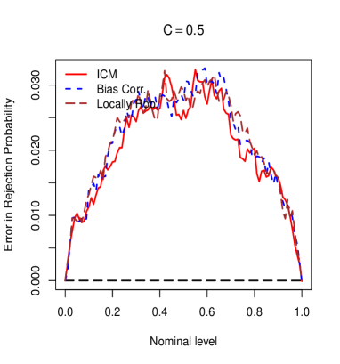
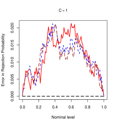
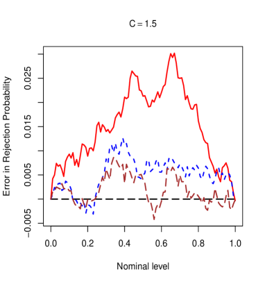
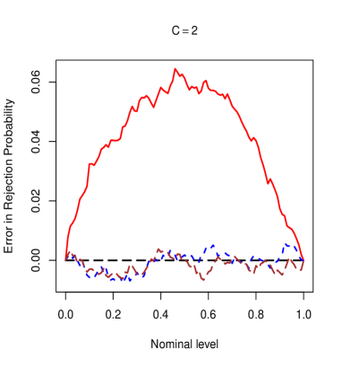
Figure 1: Errors in rejection probabilities for $n=400$ using a rule-of-thumb bandwidth $h=C\widehat{\sigma}_{W}n^{-1/5}$.

We employed Gaussian kernels of order 2 for nonparametric estimation. In a first step, we used the bandwidth rule $h=C\widehat{\sigma}_{W}n^{-1/5}$, where $\widehat{\sigma}_{W}$ is the estimated standard deviation of $W$. To check the performance of our tests under different bandwidth choices, we let the constant $C$ vary. We report actual rejection probabilities for 5% and 10% nominal sizes in Table 1. For $C=.5$ or $C=1$, the three tests have equal size control and the empirical size becomes closer to the nominal level when increasing the sample size. When $C$ increases to 1.5 then 2, size control deteriorates for the uncorrected ICM test, while it improves for our two tests. We also report in Figure 1 errors in rejection probability (ERP), that is the difference between the empirical rejection proportion and the nominal size under the null hypothesis $H_{0}$. A perfect test would exhibit an ERP of zero for any nominal size. This gives us a visual way to evaluate whether the null distribution of the test statistic is well approximated by its bootstrap approximation. These graphs clearly show the high sensitivity of the ICM test to the bandwidth choice, and the relative robustness of our two procedures. We complemented our study with an investigation of the trimming influence. While we do not report details, the most striking result we obtained was that the absence of trimming adversely affected the behavior of the locally robust test for large bandwidths.

Following the suggestion of a referee, we investigated the issue of bandwidth selection. Since there is no role for the bandwidth in the first order expansion of our test statistics, we decided to implement a data-driven bandwidth that should be asymptotically optimal for nonparametric estimation. We used an improved version of the Akaike Information Criterion proposed by Hurvich et al. (1998), which has been found to have excellent small sample performances by Li and Racine (2004). The criterion is

$$AIC_{c}=\log\left(\frac{1}{n}\sum_{i=1}^{n}[Y-\widehat{m}(W_{i})]^{2}\right)+\frac{1+tr(H)/n}{1-[tr(H)+2]/n}\,,$$

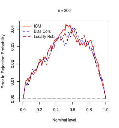
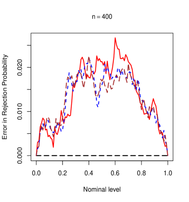
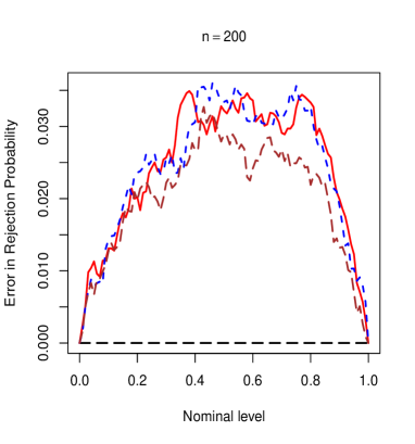
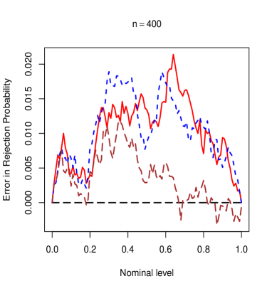
Figure 2: Errors in rejection probabilities using a data-driven bandwidth: results with trimming on first row, results with no trimming on second row.

where $H$ is the “hat matrix” such that $\left(\widehat{m}(W_{1}),\ldots,\widehat{m}(W_{n})\right)^{\prime}=H\,\left(Y_{1},\ldots,Y_{n}\right)^{\prime}$. As seen from Table 1, with this data-driven bandwidth, the three tests have good size control. We also report errors in rejection probability in Figure 2, which shows the excellent adequation of the bootstrap approximation. We then repeated our experiment without any trimming and observed that ERP are closer to zero for our tests compared to the case where trimming is implemented.

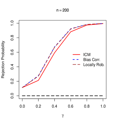
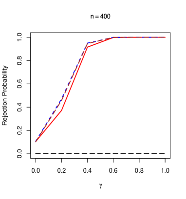
Figure 3: Power curves for tests at 10% level using a data-driven bandwidth and no trimming.

Finally, for a data-driven bandwidth and no trimming, we report in Figure 3 the power of the three tests when $\gamma$ varies. Our two tests basically have the same power, and power increases with sample size, while the uncorrected ICM test is significantly less powerful.

	$h=C\widehat{\sigma}_{W}n^{-1/5}$				Data-driven $h$
	$C=0.5$	$C=1$	$C=1.5$	$C=2$	Trimming	No trimming
$n=200$
Bias Corrected	12.15	11.13	10.35	9.83	11.34	11.43
	6.86	5.64	5.56	5.08	5.74	5.79
Locally Robust	12.08	11.05	10.39	9.71	11.48	11.27
	6.77	5.67	5.38	5.36	5.77	5.67
ICM	12.27	11.09	11.51	13.51	11.49	11.31
	6.65	5.93	6.02	7.18	6.05	6.13
$n=400$
Bias Corrected	11.41	10.74	10.31	9.43	10.70	10.64
	5.90	5.60	5.33	4.99	5.73	5.79
Locally Robust	11.32	10.73	10.17	9.70	10.81	10.24
	5.91	5.64	5.21	4.91	5.58	5.75
ICM	11.13	10.19	10.93	13.24	10.46	10.42
	6.03	5.69	5.71	6.69	5.85	5.80

Table 1: Empirical rejection percentages under $H_{0}$ at 10% and 5% nominal levels.

6.2 Empirical Illustration

We apply our encompassing tests to competing models of consumption behavior, in the spirit of Gaver and Geisel (1974) and Greene (2003, Chapter 8). The first model assumes that consumption only depends on income, and relates consumption to current and past income. The second assumes the presence of habits in consumption behavior, and relates consumption to current income and past consumption. Formally, the first model is

$$C_{i}=g_{1}(I_{i},PI_{i})+\varepsilon_{i}\,\qquad\operatorname{E}[\varepsilon_{i}|I_{i},PI_{i}]=0\,,$$ (9)

where $C_{i}$ denotes (log of) consumption of household $i$, $I_{i}$ denotes (log of) income of household $i$, and $PI_{i}$ denotes past (log of) income of household $i$. The second model is

$$C_{i}=g_{2}(I_{i},PC_{i})+\eta_{i}\,\qquad\operatorname{E}[\eta_{i}|I_{i},PC_{i}]=0\,,$$ (10)

where $PC_{i}$ denotes (log of) past consumption of household $i$.

We used data compiled by Arellano et al. (2017) from the Panel Study of Income Dynamics, which concerns $n=792$ households. We focus on the first two time periods, namely the years $1999$ and $2001$, so that $C_{i}$ and $I_{i}$ correspond to variables in 2001, while $PC_{i}$ and $PI_{i}$ correspond to 1999. We first tested if Model (9) encompasses Model (10), i.e.

$$H_{0}\,:\operatorname{E}[g_{1}(I_{i},PI_{i})\,|\,I_{i},PC_{i}]=g_{2}(I_{i},PC_{i})\,.$$ (11)

We then tested the reversed hypothesis that Model (10) encompasses Model (9), i.e.,

$$H_{0}^{\prime}\,:\,\operatorname{E}[g_{2}(I_{i},PC_{i})|I_{i},PI_{i}]=g_{1}(I_{i},PI_{i})\,.$$ (12)

We applied our encompassing tests with the bandwidth selected by the $AIC_{c}$ criterion and 999 bootstrap samples drawn to obtain critical values. Table 2 reports the values of our test statistics, together with their 95 percent bootstrap quantiles and bootstrap p-values. The first encompassing hypothesis $H_{0}$ is clearly rejected, hence Model (9) does not encompass Model (10). The encompassing hypothesis $H_{0}^{\prime}$ however cannot be rejected by any of our tests, even at a 10% nominal level. This suggests that consumption may be adequately modeled as a function of income and past consumption, in a way coherent with the consumption habit formation theory.

	Statistics	5% Critical Value	P-value
Test of $H_{0}$
Bias Corrected	3.0848	0.1820	0.0000
Locally Robust	3.1125	0.1968	0.0000
ICM	3.3948	0.2499	0.0000
Test of $H^{\prime}_{0}$
Bias Corrected	0.0069	0.0294	0.8799
Locally Robust	0.0355	0.0447	0.1912
ICM	0.0249	0.0539	0.5485

Table 2: Test of the encompassing hypotheses $H_{0}$ in (11) and $H_{0}^{\prime}$ in (12)

7 Concluding Remarks

We have studied two general approaches to obtain a small bias property for our encompassing test statistic. These approaches could potentially be used in other estimation and testing problems involving a first-step nonparametric estimation. Our simulation experiment seems to indicate that when coupled with a data-driven bandwidth these two approaches are robust to trimming choices and deliver good performances.

8 Proofs

For any real or complex valued function $g(\cdot)$, we denote with $||g||_{\infty}$ the supremum norm taken over the support of its argument and $Pg=\int g(z)\,dP(z)$. We define the population counterpart of $\widehat{t}$ as $t(w)=\mathbf{1}(f(w)\geq\tau_{n})$. By convention, $(\overline{Y}/\widehat{f})(w)$ will be set to 0 whenever $\widehat{f}(w)=0$. The same notation will hold for $\overline{\widehat{m}}/\widehat{f}$, $\overline{\phi}_{s}/\widehat{f}$, $\overline{Y^{*}}/\widehat{f}$, and $\overline{\widehat{m}^{*}}/\widehat{f}$. $C$ denotes a generic constant that may vary from line to line.

8.1 Proof of Proposition 4.2

(a) We study the bias corrected empirical process

$$\sqrt{n}\mathbb{P}_{n}(\widetilde{\varepsilon}\phi_{s}\widehat{t}) =\sqrt{n}\mathbb{P}_{n}\left(\left(Y-\widehat{m}+\widehat{B}\right)\phi_{s}\widehat{t}\right)$$

$$=\sqrt{n}\mathbb{P}_{n}(\varepsilon\phi_{s}\widehat{t})+\sqrt{n}\mathbb{P}_{n}\left((m-\widehat{m})\phi_{s}\widehat{t}\right)+\sqrt{n}\mathbb{P}_{n}(\widehat{B}\phi_{s}\widehat{t})\,.$$ (13)

Since $|\varepsilon|$ is bounded and $|\phi_{s}(\cdot)|$ is uniformly bounded,

$$\sup_{s}\left|\sqrt{n}\mathbb{P}_{n}(\varepsilon\phi_{s}(\widehat{t}-1))\right|\leq C\sqrt{n}\mathbb{P}_{n}|\widehat{t}-1|=o_{p}(1)$$

by Lemma 8.1-(i). Hence, $\sqrt{n}\mathbb{P}_{n}(\varepsilon\phi_{s}\widehat{t})=\sqrt{n}\mathbb{P}_{n}(\varepsilon\phi_{s})+o_{p}^{\mathcal{S}}(1)$, where $o_{p}^{\mathcal{S}}(1)$ denotes a uniform in $s\in{\cal S}$ $o_{p}(1)$. For the second term, as $(\widehat{t}-t)=\widehat{t}^{2}-t^{2}=(\widehat{t}+t)(\widehat{t}-t)$, and $\|(m-\widehat{m})(\widehat{t}+t)\|_{\infty}=o_{p}(n^{-1/4})$ by Lemma 8.1-(ii),

$$\sup_{s}\Big{|}\sqrt{n}\mathbb{P}_{n}(m-\widehat{m})\phi_{s}(\widehat{t}-t)\Big{|}\leq C\|(m-\widehat{m})(\widehat{t}+t)\|_{\infty}\sqrt{n}\mathbb{P}_{n}|\widehat{t}-t|=o_{p}(1)\,.$$

We now show that the third term is such that

$$\sqrt{n}\mathbb{P}_{n}(\widehat{B}\phi_{s}\widehat{t})=-\sqrt{n}\mathbb{P}_{n}(\varepsilon\iota_{s})-\sqrt{n}\mathbb{P}_{n}\left((m-\widehat{m})\iota_{s}{t}\right)+o_{p}^{\mathcal{S}}(1)\,.$$

First, use $\|\widehat{B}(\widehat{t}+t)\|_{\infty}=o_{p}(n^{-1/4})$, see Lemma 8.1-(iii), and similar arguments as above to show that $\sqrt{n}\mathbb{P}_{n}(\widehat{B}\phi_{s}\widehat{t})=\sqrt{n}\mathbb{P}_{n}(\widehat{B}\phi_{s}{t})+o_{p}^{\mathcal{S}}(1)$. Lemma 8.3-(i)-(ii) ensures in addition that $\widehat{B}\in\mathcal{G}_{l}(\mathcal{W}_{n})$ with probability approaching one, where $l=\lceil(p+1)/2\rceil$ and $\mathcal{W}_{n}:=\left\{w:f(w)\geq\tau_{n}/2\right\}$. So, Lemma 8.4-(i) yields

$$\sqrt{n}\mathbb{P}_{n}(\widehat{B}t\phi_{s}) =\sqrt{n}P(\widehat{B}t\phi_{s})+o_{p}^{\mathcal{S}}(1)\,,$$ (14)

$$P(\widehat{B}t\phi_{s}) =\int{\widehat{B}(w)t(w)\iota_{s}(w)f(w)\,dw}=P(\widehat{B}t\iota_{s})\,.$$ (15)

Since $\|[\widehat{B}-(\overline{\widehat{m}}-\overline{Y})/f]t\|_{\infty}=o_{p}(n^{-1/2})$ from Lemma 8.1-(iv) and $\iota_{s}$ is uniformly bounded,

$$\sqrt{n}P(\widehat{B}t\iota_{s}) =\sqrt{n}\int(\overline{\widehat{m}}(w)-\overline{Y}(w))t(w)\iota_{s}(w)\,dw+o_{p}^{\mathcal{S}}(1)$$

$$=-\sqrt{n}\mathbb{P}_{n}\left[(Y-\widehat{t}\widehat{m})\int K(u)(t\iota_{s})(W+uh)\,du\right]+o_{p}^{\mathcal{S}}(1)$$

$$=-\sqrt{n}\mathbb{P}_{n}\left[\left(\varepsilon-(\widehat{m}-m)\widehat{t}-m(\widehat{t}-1)\right)\int K(u)(t\iota_{s})(W+uh)\,du\right]+o_{p}^{\mathcal{S}}(1)\,,$$

where the second equality follows from a change of variable. Let us deal with each term separately. Since $\varepsilon$ is bounded and $|t(w+uh)-1|=\mathbf{1}\{f(w+uh)<\tau_{n}\}$,

$$\Big{|}\sqrt{n}\mathbb{P}_{n}\varepsilon\int K(u)\iota_{s}(W+uh) [t(W+uh)-1]\,du\Big{|}\leq C\int|K(u)|\sqrt{n}\mathbb{P}_{n}\mathbf{1}\left\{f(W+uh)<\tau_{n}\right\}\,du\,.$$

By a mean-value expansion, for all $(u,w)\in\text{Supp}(K)\times\mathbb{R}^{p}$ we have $f(w+hu)-f(w)=\partial^{T}f(\widetilde{w})uh$, for some $\widetilde{w}$. By Assumptions A-B, $\left|\partial^{T}f(w)uh\right|\leq Ch\quad\text{for all }(u,w)\in\text{Supp}(K)\times\mathbb{R}^{p}$. Since $h\tau_{n}^{-1}=o(1)$, for $n$ large enough $\mathbf{1}\{f(w+uh)<\tau_{n}\}\leq\mathbf{1}\{f(w)\leq 3\tau_{n}/2\}$. Now use $\mathbb{P}_{n}\mathbf{1}\Big{\{}f(W)\leq 3\tau_{n}/2\Big{\}}=O_{P}(p_{n})=o_{P}(n^{-1/2})$, from Assumption D(i), to obtain

$$\sqrt{n}\mathbb{P}_{n}\left[\varepsilon\int K(u)(t\iota_{s})(W+uh)\,du\right]=\sqrt{n}\mathbb{P}_{n}\left[\varepsilon\int K(u)\iota_{s}(W+uh)\,du\right]+o_{p}^{\mathcal{S}}(1)\,.$$

The same reasoning allows the same replacement in the second and third term of the decomposition, using that $\|(\widehat{m}-m)\widehat{t}\|_{\infty}$ is $o_{p}(1)$ by Lemma 8.1-(ii) and that $m(\widehat{t}-1)$ is bounded.

Then

$$\sqrt{n}P(\widehat{B}t\iota_{s}) =-\sqrt{n}\mathbb{P}_{n}\left[\varepsilon\int K(u)\iota_{s}(W+uh)\,du\right]+\sqrt{n}\mathbb{P}_{n}\left[(\widehat{m}-m)\widehat{t}\int K(u)\iota_{s}(W+uh)\,du\right]$$

$$+\sqrt{n}\mathbb{P}_{n}\left[m(\widehat{t}-1)\int K(u)\iota_{s}(W+uh)\,du\right]+o_{p}^{\mathcal{S}}(1)\,.$$ (16)

Lemma 8.4(ii) yields

$$\sqrt{n}\mathbb{P}_{n}\left(\varepsilon\int K(u)\iota_{s}(W+uh)\,du\right)=\sqrt{n}\mathbb{P}_{n}(\varepsilon\iota_{s})+o_{p}^{\mathcal{S}}(1)\,,$$

as $P\left(\varepsilon\int K(u)\iota_{s}(W+uh)\,du\right)=P\left(\varepsilon\iota_{s}\right)=0$. A Taylor expansion of order $r$ guarantees that $\int K(u)\iota_{s}(w+uh)du=\iota_{s}(w)+O(h^{r})$ uniformly in $\mathcal{S}\times\mathcal{W}$ as $\iota_{s}(\cdot)$ has uniformly bounded derivatives of order $r$. Since $\|(\widehat{m}-m)\widehat{t}\|_{\infty}=o_{p}(n^{-1/4})$ and $nh^{4r}=o(1)$,

$$\sqrt{n}\mathbb{P}_{n}\left((\widehat{m}-m)\widehat{t}\int K(u)\iota_{s}(W+uh)\,du\right) =\sqrt{n}\mathbb{P}_{n}((\widehat{m}-m)\widehat{t}\iota_{s})+o_{p}^{\mathcal{S}}(1)\,.$$

Now use similar arguments as before to replace $\widehat{t}$ by $t$. The last term in (16) is negligible. Indeed, the argument of $\mathbb{P}_{n}$ is uniformly bounded, and $\sqrt{n}\mathbb{P}_{n}|t-1|=o_{P}(1)$ from Lemma 8.1-(i). Hence,

$$\sqrt{n}P(\widehat{B}t\iota_{s}) =-\sqrt{n}\mathbb{P}_{n}(\varepsilon\iota_{s})+\sqrt{n}\mathbb{P}_{n}((\widehat{m}-m){t}\iota_{s})+o_{p}^{\mathcal{S}}(1)\,.$$

Gathering results,

$$\sqrt{n}\mathbb{P}_{n}(\widetilde{\varepsilon}\phi_{s}\widehat{t})=\sqrt{n}\mathbb{P}_{n}(\varepsilon(\phi_{s}-\iota_{s}))+\sqrt{n}\mathbb{P}_{n}\left((m-\widehat{m})(\phi_{s}-\iota_{s}){t}\right)+o_{p}^{\mathcal{S}}(1)\,.$$

From arguments similar to those used for (14), since $\|(m-\widehat{m})t\|_{\infty}=o_{p}(n^{-1/4})$ and $\widehat{m}\in\mathcal{G}_{l}(\mathcal{W}_{n})$ with probability approaching one,

$$\sqrt{n}\mathbb{P}_{n}\left((m-\widehat{m})(\phi_{s}-\iota_{s}){t}\right)=\sqrt{n}P\left((m-\widehat{m})(\phi_{s}-\iota_{s}){t}\right)+o_{p}^{\mathcal{S}}(1)\,.$$

But $\sqrt{n}P\left((m-\widehat{m})(\phi_{s}-\iota_{s}){t}\right)=0$ as $\operatorname{E}(\phi_{s}(X)|W)=\iota_{s}(W)$. Finally, we obtain $\sqrt{n}\mathbb{P}_{n}(\widetilde{\varepsilon}\phi_{s}\widehat{t})=\sqrt{n}\mathbb{P}_{n}(\varepsilon(\phi_{s}-\iota_{s}))+o_{p}^{\mathcal{S}}(1)$ as expected.

(b) We now study the locally robust empirical process

$$\sqrt{n}\mathbb{P}_{n}(\widehat{\varepsilon}(\phi_{s}-\widehat{\iota}_{s})\widehat{t}) =\sqrt{n}\mathbb{P}_{n}\left(\left(Y-\widehat{m}\right)(\phi_{s}-\widehat{\iota}_{s})\widehat{t}\right)$$

$$=\sqrt{n}\mathbb{P}_{n}(\varepsilon(\phi_{s}-\widehat{\iota}_{s})\widehat{t})+\sqrt{n}\mathbb{P}_{n}\left((m-\widehat{m})(\phi_{s}-\widehat{\iota}_{s})\widehat{t}\right)\,.$$ (17)

A similar reasoning as in Part (a) allows replacing $\widehat{t}$ by $t$ and yields

$$\sqrt{n}\mathbb{P}_{n}(\widehat{\varepsilon}(\phi_{s}-\widehat{\iota}_{s})\widehat{t}) =\sqrt{n}\mathbb{P}_{n}(\varepsilon(\phi_{s}-\widehat{\iota}_{s}){t})+\sqrt{n}\mathbb{P}_{n}\left((m-\widehat{m})(\phi_{s}-\widehat{\iota}_{s}){t}\right)+o_{p}^{\mathcal{S}}(1)\,,$$

based on the boundedness of $\varepsilon$, $\sqrt{n}\mathbb{P}_{n}|\widehat{t}-t|=o_{p}(1)$, and the boundedness in probability of $\sup_{s}\|(\phi_{s}-\widehat{\iota}_{s}){t}\|_{\infty}$, $\sup_{s}\|(\phi_{s}-\widehat{\iota}_{s})\widehat{t}\|_{\infty}$, $\|(\widehat{m}-m)t\|_{\infty}$, and $\|(\widehat{m}-m)\widehat{t}\|_{\infty}$, see Lemma 8.1. From Lemma 8.1, $\sup_{s}\|(\widehat{\iota}_{s}-\iota_{s})t\|_{\infty}=o_{p}(n^{-1/4})$ and $\|(m-\widehat{m})t\|_{\infty}=o_{P}(n^{-1/4})$, hence

$$\sqrt{n}\mathbb{P}_{n}\left((m-\widehat{m})(\phi_{s}-\widehat{\iota}_{s}){t}\right)=\sqrt{n}\mathbb{P}_{n}\left((m-\widehat{m})(\phi_{s}-{\iota}_{s}){t}\right)+o_{p}^{\mathcal{S}}(1)=o_{p}^{\mathcal{S}}(1)\,,$$

where the last equality is established in Part (a). Now,

$$\mathbb{P}_{n}\varepsilon(\phi_{s}-\widehat{\iota}_{s})t=\mathbb{P}_{n}\varepsilon(\phi_{s}-\iota_{s})t-\mathbb{P}_{n}\varepsilon(\widehat{\iota}_{s}-\iota_{s})t\,,$$

and $\sup_{s}\left|\sqrt{n}\mathbb{P}_{n}(\varepsilon(\phi_{s}-\iota_{s})(t-1))\right|\leq C\sqrt{n}\mathbb{P}_{n}|t-1|=o_{P}(1)$ by Lemma 8.1-(i). Last, $\sqrt{n}\mathbb{P}_{n}\varepsilon(\widehat{\iota}_{s}-\iota_{s})t=o_{p}^{\mathcal{S}}(1)$ by Lemma 8.4-(i). Gathering results, $\sqrt{n}\mathbb{P}_{n}(\widehat{\varepsilon}(\phi_{s}-\widehat{\iota}_{s})\widehat{t})=\sqrt{n}\mathbb{P}_{n}({\varepsilon}(\phi_{s}-{\iota}_{s}))+o_{p}^{\mathcal{S}}(1)$.

8.2 Proof of Proposition 5.1

We here consider statements relative to $P^{\xi}\otimes P$, the joint probability measure of both the bootstrap weights and the sample data.

(a) We study the bootstrap version of the bias corrected empirical process

$$\sqrt{n}\mathbb{P}_{n}(\widetilde{\varepsilon}^{*}\phi_{s}\widehat{t}) =\sqrt{n}\mathbb{P}_{n}\left(\left(Y^{*}-\widehat{m}^{*}+\widehat{B}^{*}\right)\phi_{s}\widehat{t}\right)$$

$$=\sqrt{n}\mathbb{P}_{n}(\xi\varepsilon\phi_{s}\widehat{t})+\sqrt{n}\mathbb{P}_{n}\left(\xi(m-\widehat{m})\phi_{s}\widehat{t}\right)+\sqrt{n}\mathbb{P}_{n}\left((\widehat{m}-\widehat{m}^{*})\phi_{s}\widehat{t}\right)+\sqrt{n}\mathbb{P}_{n}(\widehat{B}^{*}\phi_{s}\widehat{t})\,.$$

From here we only stress the differences with the proof of Proposition 1. Proceeding as in the latter proof and using results in Lemma 8.1,

$$\sqrt{n}\mathbb{P}_{n}(\xi\varepsilon\phi_{s}\widehat{t}) =\sqrt{n}\mathbb{P}_{n}(\xi\varepsilon\phi_{s}{t})+o_{P}^{\mathcal{S}}(1)\,,$$

$$\sqrt{n}\mathbb{P}_{n}\left(\xi(m-\widehat{m})\phi_{s}\widehat{t}\right) =\sqrt{n}\mathbb{P}_{n}\left(\xi(m-\widehat{m})\phi_{s}{t}\right)+o_{P}^{\mathcal{S}}(1)\,,$$

$$\sqrt{n}\mathbb{P}_{n}\left((\widehat{m}-\widehat{m}^{*})\phi_{s}\widehat{t}\right) =\sqrt{n}\mathbb{P}_{n}\left((\widehat{m}-\widehat{m}^{*})\phi_{s}{t}\right)+o_{P}^{\mathcal{S}}(1)\,,$$

$$\sqrt{n}\mathbb{P}_{n}(\widehat{B}^{*}\phi_{s}\widehat{t}) =\sqrt{n}\mathbb{P}_{n}(\widehat{B}^{*}\phi_{s}{t})+o_{P}^{\mathcal{S}}(1)\,.$$

For the last term, use $\|\widehat{B}^{*}t\|_{\infty}=o_{P}(n^{-1/4})$, Lemma 8.3-(ii)-(iv)-(v), and Lemma 8.4-(i) to show that

$$\sqrt{n}\mathbb{P}_{n}(\widehat{B}^{*}t\phi_{s})=\sqrt{n}P(\widehat{B}^{*}t\phi_{s})+o_{P}^{\mathcal{S}}(1)\,.$$ (18)

From the law of iterated expectations, $P(\widehat{B}^{*}t\phi_{s})=P(\widehat{B}^{*}t\iota_{s})$. Since $\|[\widehat{B}^{*}-(\overline{\widehat{m}^{*}}-\overline{Y^{*}})/f]t\|_{\infty}=o_{P}(n^{-1/2})$ from Lemma 8.1-(viii),

$$\sqrt{n}P(\widehat{B}^{*}t\iota_{s}) =\sqrt{n}\int(\overline{\widehat{m}^{*}}(w)-\overline{Y^{*}}(w))t(w)\iota_{s}(w)\,dw+o_{P}^{\mathcal{S}}(1)$$

$$=-\sqrt{n}\mathbb{P}_{n}\left[(Y^{*}-\widehat{m}^{*})\widehat{t}\int K(u)(t\iota_{s})(W+uh)\,du\right]+o_{P}^{\mathcal{S}}(1)\,,$$

where the second equality follows from a change of variable. Replace $(Y^{*}-\widehat{m}^{*})\widehat{t}$ by $\xi\varepsilon{t}+\xi\varepsilon(\widehat{t}-t)+\xi(m-\widehat{m})\widehat{t}+(\widehat{m}-\widehat{m}^{*})\widehat{t}$ and proceed as in Proposition 1 to obtain

$$\sqrt{n}P(\widehat{B}^{*}t\phi_{s}) =-\sqrt{n}\mathbb{P}_{n}(\xi\varepsilon\iota_{s}t)-\sqrt{n}\mathbb{P}_{n}((\widehat{m}-\widehat{m}^{*}){t}\iota_{s})-\sqrt{n}\mathbb{P}_{n}\xi(m-\widehat{m})t\iota_{s}+o_{P}^{\mathcal{S}}(1)\,.$$

Gathering results,

$$\sqrt{n}\mathbb{P}_{n}(\widetilde{\varepsilon}^{*}\phi_{s}\widehat{t})= \sqrt{n}\mathbb{P}_{n}(\xi\varepsilon(\phi_{s}-\iota_{s}){t})+\sqrt{n}\mathbb{P}_{n}\left(\xi(m-\widehat{m})(\phi_{s}-\iota_{s}){t}\right)$$

$$\qquad+\sqrt{n}\mathbb{P}_{n}((\widehat{m}-\widehat{m}^{*})t(\phi_{s}-\iota_{s}))+o_{P}^{\mathcal{S}}(1)\,.$$

A reasoning similar to Proposition 1 then yields $\sqrt{n}\mathbb{P}_{n}(\xi\varepsilon(\phi_{s}-\iota_{s}))t=\sqrt{n}\mathbb{P}_{n}(\xi\varepsilon(\phi_{s}-\iota_{s}))+o_{P}^{\mathcal{S}}(1)$, $\sqrt{n}\mathbb{P}_{n}\left(\xi(m-\widehat{m})(\phi_{s}-\iota_{s}){t}\right)=o_{P}^{\mathcal{S}}(1)$, and $\sqrt{n}\mathbb{P}_{n}((\widehat{m}-\widehat{m}^{*})t(\phi_{s}-\iota_{s}))=o_{P}^{\mathcal{S}}(1)$. Hence

$$\sqrt{n}\mathbb{P}_{n}\widetilde{\varepsilon}^{*}\widehat{t}\phi_{s}=\sqrt{n}\mathbb{P}_{n}\xi\varepsilon(\phi_{s}-\iota_{s})+o_{P}^{\mathcal{S}}(1).$$

For the locally robust empirical process,

$$\sqrt{n}\mathbb{P}_{n}(\widehat{\varepsilon}^{*}(\phi_{s}-\widehat{\iota}_{s})\widehat{t}) =\sqrt{n}\mathbb{P}_{n}(\xi\varepsilon(\phi_{s}-\widehat{\iota}_{s})\widehat{t})$$

$$+\sqrt{n}\mathbb{P}_{n}\left(\xi(m-\widehat{m})(\phi_{s}-\widehat{\iota}_{s})\widehat{t}\right)+\sqrt{n}\mathbb{P}_{n}\left((\widehat{m}-\widehat{m}^{*})(\phi_{s}-\widehat{\iota}_{s})\widehat{t}\right)\,.$$

The proof proceeds along similar lines to show that the first term equals $\sqrt{n}\mathbb{P}_{n}(\xi\varepsilon(\phi_{s}-{\iota}_{s}))+o_{P}^{\mathcal{S}}(1)$ and the other terms are both $o_{P}^{\mathcal{S}}(1)$.

(b) Since the class $\{(y,w,x)\mapsto(y-m(w))(\phi_{s}(x)-\iota_{s}(w)):s\in\mathcal{S}\}$ is Donsker, $\sqrt{n}\mathbb{P}_{n}\varepsilon(\phi_{s}-\iota_{s})$ converges weakly to a tight zero-mean Gaussian process $\mathbb{G}_{s}$ under $H_{0}$, see the main text. By the continuity of the Cramer-Von Mises functional and Proposition 1, $S_{n}^{BC}$ and $S_{n}^{LR}$ weakly converge to $\int|\mathbb{G}_{s}|^{2}\mu(ds)$. From Bentkus et al. (1993), this distribution is continuous, so pointwise convergence implies uniform convergence.

Using van der Vaart and Wellner (2000, Theorem 2.9.6), we get weak convergence of $\sqrt{n}\mathbb{P}_{n}\xi\varepsilon(\phi_{s}-\iota_{s})$ in probability conditionally upon the initial sample to a tight zero-mean Gaussian process $\mathbb{G}^{\prime}_{s}$ with the same covariance function as $\mathbb{G}_{s}$. From (a), the bootstrap statistics (8) weakly converge to $\int|\mathbb{G}^{\prime}_{s}|^{2}\mu(ds)$ in probability conditionally upon the initial sample. The desired result then follows.

(c) From (a) and a Glivenko-Cantelli property of the class $\{(y,w,x)\mapsto(y-m(w))(\phi_{s}(x)-\iota_{s}(w)):s\in\mathcal{S}\}$, $\mathbb{P}_{n}\widetilde{\varepsilon}\widehat{t}\phi_{s}=P\varepsilon(\phi_{s}-\iota_{s})+o_{P}^{\mathcal{S}}(1)$ and similarly for $\mathbb{P}_{n}\widehat{\varepsilon}(\phi_{s}-\widehat{\iota})\widehat{t}$. Hence, $S_{n}^{LR}/n$ and $S_{n}^{BC}/n\mbox{$\stackrel{{\scriptstyle p}}{{\longrightarrow}}\,$}\int|\operatorname{E}\varepsilon(\phi_{s}-\iota_{s})|^{2}d\mu(s)$. From Bierens (2017, Theorem 2.2), under $H_{1}$, $\operatorname{E}\varepsilon(\phi_{s}-\iota_{s})\neq 0$ for almost all $s$ and $\int\left|\operatorname{E}\varepsilon(\phi_{s}-\iota_{s})\right|^{2}\,d\mu(s)>0$. From (b), it holds that the bootstrap statistics are bounded in probability, and the result follows.

8.3 Auxiliary Lemmas

Lemma 8.1.

Under Assumptions A-D,

1. $\mathbb{P}_{n}|t-1|=o_{p}(n^{-1/2})$ and $\mathbb{P}_{n}|\widehat{t}-t|=o_{p}(n^{-1/2})$,

2. $\|(\widehat{m}-m)t\|_{\infty}=o_{p}(n^{-1/4})$ and $\|(\widehat{m}-m)\widehat{t}\|_{\infty}=o_{p}(n^{-1/4})$,

3. $\|\widehat{B}t\|_{\infty}=o_{p}(n^{-1/4})$ and $\|\widehat{B}\widehat{t}\|_{\infty}=o_{p}(n^{-1/4})$,

4. $\|[\widehat{B}-(\overline{\widehat{m}}-\overline{Y})/f]t\|_{\infty}=o_{p}(n^{-1/2})$,

5. $\sup_{s}\|(\widehat{\iota}_{s}-\iota_{s})t\|_{\infty}=o_{p}(n^{-1/4})$ and $\sup_{s}\|(\widehat{\iota}_{s}-\iota_{s})\widehat{t}\|_{\infty}=o_{p}(n^{-1/4})$,

6. $\|(\widehat{m}^{*}-m)t\|_{\infty}=o_{P}(n^{-1/4})$ and $\|(\widehat{m}^{*}-m)\widehat{t}\|_{\infty}=o_{P}(n^{-1/4})$,

7. $\|\widehat{B}^{*}t\|_{\infty}=o_{P}(n^{-1/4})$ and $\|\widehat{B}^{*}\widehat{t}\|_{\infty}=o_{P}(n^{-1/4})$,

8. $\|[\widehat{B}^{*}-(\overline{\widehat{m}^{*}}-\overline{Y^{*}})/f]t\|_{\infty}=o_{P}(n^{-1/2})$.

Proof.

$(i)$ Notice first that $|t-1|=\mathbf{1}(f(\cdot)<\tau_{n})$ and

$$\operatorname{E}\mathbb{P}_{n}\mathbf{1}(f(W)<\tau_{n})\leq\text{Pr}(f(W)\leq 3\tau_{n}/2)=p_{n}=o(n^{-1/2})$$

where the last equality follows from Assumption D(i). So, by Markov’s inequality, $\mathbb{P}_{n}|t-1|=o_{P}(n^{-1/2})$.
To prove the second part of $(i)$, define the event $\mathcal{A}_{C}:=\{\|\widehat{f}-f\|_{\infty}\leq Cd_{n}\}$. From Lemma 8.2 $\|\widehat{f}-\operatorname{E}\widehat{f}\|_{\infty}=O_{P}(\sqrt{(\log n)/(nh^{p})})$. Standard bias manipulations ensure that $\|\operatorname{E}\widehat{f}-f\|_{\infty}=O(h^{r})$. So, $\|\widehat{f}-f\|_{\infty}=O(d_{n})$ and by choosing $C$ large enough $\text{Pr}(\mathcal{A}_{C})$ can be made arbitrarily close to 1 for each large $n$. Over such event, since $d_{n}\tau_{n}^{-1}=o(1)$ (see Assumption C), for each $n$ large enough $1-\tau_{n}^{-1}(\widehat{f}(w)-f(w))\leq 3/2$ for all $w\in\mathcal{W}$. Thus,

$$\mathbf{1}\Big{(}\widehat{f}(w)\geq\tau_{n}\Big{)}=\mathbf{1}\Big{(}f(w)\geq\tau_{n}\Big{[}1-\frac{\widehat{f}(w)-f(w)}{\tau_{n}}\Big{]}\Big{)}\geq\mathbf{1}\Big{(}f(w)\geq 3\tau_{n}/2\Big{)}$$

so that $f(w)\geq(3/2)\tau_{n}$ implies $t(w)=\widehat{t}(w)=1$. Accordingly, over $\mathcal{A}_{C}$ for large enough $n$

$$|\widehat{t}(w)-t(w)|\leq\mathbf{1}\Big{(}f(w)<3\tau_{n}/2\Big{)}\text{ for all }w\in\mathcal{W}\,$$

and

$$\mathbb{P}_{n}|\widehat{t}-t|\leq\mathbb{P}_{n}\mathbf{1}\Big{(}f(W)<3\tau_{n}/2\Big{)}=O_{P}(p_{n})=o_{P}(n^{-1/2})\,,$$

where the last two equalities follow from Markov’s inequality and Assumption D(i). Conclude by recalling that for $C$ large enough $\text{Pr}(\mathcal{A}_{C})$ can be made arbitrarily close to 1 for each large $n$.

$(ii)$ Consider the event $\mathcal{A}_{C}$ previously defined and fix $\delta\in(0,1]$. Since $d_{n}\tau_{n}^{-1}=o(1)$, over such event for each large $n$ we have $1+2[f(w)-\widehat{f}(w)]/(\delta\tau_{n})\leq 2$ for all $w\in\mathcal{W}$. So,

$$\mathbf{1}\Big{(}\widehat{f}(w)\geq\delta\tau_{n}/2\Big{)}=\mathbf{1}\Big{(}f(w)\geq\frac{\delta\tau_{n}}{2}\Big{[}1+2\frac{f(w)-\widehat{f}(w)}{\delta\tau_{n}}\Big{]}\Big{)}\geq\mathbf{1}\Big{(}f(w)\geq\delta\tau_{n}\Big{)}.$$

As already seen, by choosing $C$ large enough $\text{Pr}(\mathcal{A}_{C})$ can be made arbitrarily close to 1 for each large $n$. So, we obtain that

$$\text{ for each $\delta\in(0,1]$ wpa1 : }\mathbf{1}\Big{(}f(w)\geq\delta\tau_{n}\Big{)}\leq\mathbf{1}\Big{(}\widehat{f}(w)\geq\delta\tau_{n}/2\Big{)}\text{ for all }w\in\mathcal{W},$$ (19)

where wpa1 stands for ”with probability approaching one”. Switching the roles of $\widehat{f}$ and $f$, by a similar argument we obtain that

$$\text{ for each $\delta\in(0,1]$ wpa1 : }\mathbf{1}\Big{(}\widehat{f}(w)\geq\delta\tau_{n}\Big{)}\leq\mathbf{1}\Big{(}f(w)\geq\delta\tau_{n}/2\Big{)}\text{ for all }w\in\mathcal{W}.$$ (20)

Now, for any fixed $\delta\in(0,1]$ (19) implies that with probability approaching one

$$(\widehat{m}-m)\text{ }\mathbf{1}(f(\cdot)\geq\delta\tau_{n})= \frac{\overline{Y}-m\widehat{f}}{f}\text{ }\mathbf{1}(f(\cdot)\geq\delta\tau_{n})$$

$$+\frac{\overline{Y}-m\widehat{f}}{f}\text{ }\frac{f-\widehat{f}}{\widehat{f}}\text{ }\mathbf{1}(f(\cdot)\geq\delta\tau_{n})\text{ }\mathbf{1}(\widehat{f}(\cdot)\geq\delta\tau_{n}/2)\,.$$

To bound the RHS, from Lemma 8.2 $\|\overline{Y}-\operatorname{E}\overline{Y}\|_{\infty}=O_{P}(\sqrt{(\log n)/(nh^{p})})$, while standard bias computations yield $\|\operatorname{E}\overline{Y}-mf\|_{\infty}=O(h^{r})$. Hence, $\|\overline{Y}-mf\|_{\infty}=O_{P}(d_{n})$. Similarly, $\|\widehat{f}-f\|_{\infty}=O_{P}(d_{n})$ . Using these rates and the above display gives

$$\|(\widehat{m}-m)\text{ }\mathbf{1}(f(\cdot)\geq\delta\tau_{n})\|_{\infty}=O_{P}\left(\frac{d_{n}}{\tau_{n}}+\frac{d_{n}^{2}}{\tau_{n}^{2}}\right)=o_{P}(n^{-1/4})$$ (21)

where the last equality follows from Assumption C. Since $\delta\in(0,1]$, the LHS of the above display is an upper bound for $\|(\widehat{m}-m)t\|_{\infty}$. So $\|(\widehat{m}-m)t\|_{\infty}=o_{P}(n^{-1/4})$. To obtain the rate with $\widehat{t}$, an application of (20) with $\delta=1$ gives that with probability approaching one $\|(\widehat{m}-m)\widehat{t}\|_{\infty}\leq\|(\widehat{m}-m)\text{ }\mathbf{1}(f(\cdot)\geq\tau_{n}/2)\|_{\infty}$. Applying (21) with $\delta=1/2$ gives the $n^{-1/4}$ rate for the RHS of the latter inequality.

$(iii)$ Since $\widehat{B}=\overline{\widehat{m}}/\widehat{f}-\widehat{m}$, in view of $(ii)$ it suffices to obtain a rate for $\overline{\widehat{m}}/\widehat{f}$. To this end, notice that

$$\overline{\widehat{m}}(w)=\overline{m}(w)+\overline{m(\widehat{t}-1)}(w)+\overline{(\widehat{m}-m)\widehat{t}}(w)\,.$$ (22)

Combining Lemma 8.2 with standard bias computations gives $\|\overline{m}-mf\|_{\infty}=O_{P}(d_{n})$. For the second term, the boundedness of $K$ and $m$ implies $|\overline{m(\widehat{t}-1)}(w)|\leq Ch^{-p}\mathbb{P}_{n}|\widehat{t}-1|$. Using the same arguments as in the proof of $(i)$, $\mathbb{P}_{n}|\widehat{t}-1|\leq\mathbb{P}_{n}|\widehat{t}-t|+\mathbb{P}_{n}|t-1|=O_{P}(p_{n})$. So, $\|\overline{m(\widehat{t}-1)}\|_{\infty}=O_{P}(p_{n}h^{-p})$. For the third term on the RHS of (22)

$$\overline{(\widehat{m}-m)\widehat{t}}(w)\leq\|(\widehat{m}-m)\widehat{t}\|_{\infty}h^{-p}\mathbb{P}_{n}\Big{|}K\Big{(}\frac{W-w}{h}\Big{)}\Big{|}=O_{P}\Big{(}\frac{d_{n}}{\tau_{n}}\Big{)}\cdot h^{-p}\mathbb{P}_{n}\Big{|}K\Big{(}\frac{W-w}{h}\Big{)}\Big{|}$$

where in the last equality we have used $\left\|(\widehat{m}-m)\widehat{t}\right\|_{\infty}=O_{P}(d_{n}/\tau_{n})$ from the proof of $(ii)$. An application of Lemma 8.2 and standard bias computations yield that the last term on the RHS is $O_{P}(1)$ uniformly in $w\in\mathcal{W}$. Gathering results,

$$\|\overline{\widehat{m}}-mf\|_{\infty}=O_{P}\left(d_{n}+p_{n}h^{-p}+\frac{d_{n}}{\tau_{n}}\right)\,.$$ (23)

Combining the above display with arguments similar to the proof of $(ii)$ gives

$$\left\|\left(\frac{\overline{\widehat{m}}}{\widehat{f}}-m\right)\widehat{t}\right\|_{\infty}=O_{P}\left(\frac{d_{n}}{\tau_{n}^{2}}+\frac{p_{n}}{h^{p}\tau_{n}}\right)\text{ and }\left\|\left(\frac{\overline{\widehat{m}}}{\widehat{f}}-m\right){t}\right\|_{\infty}=O_{P}\left(\frac{d_{n}}{\tau_{n}^{2}}+\frac{p_{n}}{h^{p}\tau_{n}}\right)\,.$$ (24)

Using Assumption C and D(i) gives the desired result.

$(iv)$ Since $\widehat{B}=\overline{\widehat{m}}/\widehat{f}-\overline{Y}/\widehat{f}$, Equation (19) implies that with probability approaching one

$$\Big{(}\widehat{B}-\frac{\overline{\widehat{m}}-\overline{Y}}{f}\Big{)}\text{ }t=(\overline{\widehat{m}}-\overline{Y})\Big{(}\frac{f-\widehat{f}}{\widehat{f}f}\text{ }\Big{)}\text{ }t\text{ }\mathbf{1}(\widehat{f}(\cdot)\geq\tau_{n}/2)\,.$$

Using (23), $\|\overline{Y}-mf\|_{\infty}=O_{P}(d_{n})$, and $\|\widehat{f}-f\|_{\infty}=O_{P}(d_{n})$ (see the proof of $(ii)$), the RHS of the above display is

$$O_{P}\Big{(}\Big{(}\frac{d_{n}}{\tau_{n}^{2}}+\frac{p_{n}}{h^{p}\tau_{n}}\Big{)}\text{ }\frac{d_{n}}{\tau_{n}}\Big{)}=o_{P}(n^{-1/2})$$

uniformly in $w\in\mathcal{W}$, where the last equality follows from Assumptions C and D(i).

$(v)$ The proof follows from arguments similar to the proof of $(ii)$, so it is omitted.

$(vi)$ First, notice that

$$\widehat{m}^{*}=\frac{\overline{Y^{*}}}{\widehat{f}}=\frac{\overline{\widehat{m}}}{\widehat{f}}+\frac{\overline{\xi\widehat{\varepsilon}}}{\widehat{f}}.$$ (25)

The uniform convergence rate of $\overline{\widehat{m}}/\widehat{f}$ has already been obtained in (24), so it suffices to show that the second addendum is negligible with a suitable rate. Now, $\overline{\xi\widehat{\varepsilon}}=\overline{\xi\varepsilon}+\overline{\xi\varepsilon(\widehat{t}-1)}+\overline{\xi(m-\widehat{m})\widehat{t}}$. Using this decomposition and proceeding as in the proof of $(iii)$ gives

$$\left\|\frac{\overline{\xi\widehat{\varepsilon}}}{\widehat{f}}\widehat{t}\right\|_{\infty}=O_{P}\left(\frac{d_{n}}{\tau_{n}^{2}}+\frac{p_{n}}{h^{p}\tau_{n}}\right)\text{ and }\left\|\frac{\overline{\xi\widehat{\varepsilon}}}{\widehat{f}}{t}\right\|_{\infty}=O_{P}\left(\frac{d_{n}}{\tau_{n}^{2}}+\frac{p_{n}}{h^{p}\tau_{n}}\right)$$ (26)

with $d_{n}\tau_{n}^{-2}+p_{n}h^{-p}\tau_{n}^{-1}=o(n^{-1/4})$.

$(vii)$ Recall that

$$\widehat{B}^{*}=\frac{\overline{\widehat{m}^{*}}}{\widehat{f}}-\widehat{m}^{*}\text{ . }$$

In view of $(iv)$, it suffices to obtain a suitable convergence rate for the first addendum. To this end, from (24), (25), and (26) we have

$$\|(\widehat{m}^{*}-m)\widehat{t}\|_{\infty}=O_{P}\left(\frac{d_{n}}{\tau_{n}^{2}}+\frac{p_{n}}{h^{p}\tau_{n}}\right)\text{ .}$$ (27)

Also, $\overline{\widehat{m}^{*}}=\overline{m}+\overline{m(\widehat{t}-1)}+\overline{(\widehat{m}^{*}-m)\widehat{t}}$. Using this decomposition, (27), and proceeding similarly as in the proof of $(iii)$ gives

$$\left\|\left(\frac{\widehat{m}^{*}}{\widehat{f}}-m\right)\widehat{t}\right\|_{\infty}=O_{P}\left(\frac{d_{n}}{\tau_{n}^{3}}+\frac{p_{n}}{h^{p}\tau_{n}^{2}}\right)\text{ and }\left\|\left(\frac{\widehat{m}^{*}}{\widehat{f}}-m\right){t}\right\|_{\infty}=O_{P}\left(\frac{d_{n}}{\tau_{n}^{3}}+\frac{p_{n}}{h^{p}\tau_{n}^{2}}\right)\text{ . }$$

By Assumptions C and D(i) we obtain the desired result.

$(viii)$ The proof combines arguments already used previously. For completeness, we also provide it here. Using the definition of $\widehat{B}^{*}$ and (19), with probability approaching one

$$\Big{(}\widehat{B}^{*}-\frac{\overline{\widehat{m}^{*}}-\overline{Y^{*}}}{f}\Big{)}\text{ }t=(\overline{\widehat{m}^{*}}-\overline{Y^{*}})\Big{(}\frac{f-\widehat{f}}{f\widehat{f}}\Big{)}\text{ }t\text{ }\mathbf{1}(\widehat{f}(\cdot)\geq\tau_{n}/2)\text{ .}$$ (28)

As noticed in the proof of $(vii)$, $\overline{\widehat{m}^{*}}=\overline{m}+\overline{m(\widehat{t}-1)}+\overline{(\widehat{m}^{*}-m)\widehat{t}}$. By this decomposition, (27), and reasoning as in the proof of $(iii)$ we get

$$\|\overline{\widehat{m}^{*}}-mf\|_{\infty}=O_{P}\Big{(}\frac{d_{n}}{\tau_{n}^{2}}+\frac{p_{n}}{h^{p}\tau_{n}}\Big{)}.$$ (29)

Combining $\overline{\xi\widehat{\varepsilon}}=\overline{\xi\varepsilon}+\overline{\xi\varepsilon(\widehat{t}-1)}+\overline{\xi(m-\widehat{m})\widehat{t}}$ with arguments used in the proof of $(iii)$ gives

$$\|\overline{\xi\widehat{\varepsilon}}\|_{\infty}=O_{P}\left(\frac{d_{n}}{\tau_{n}}+\frac{p_{n}}{h^{p}}\right).$$

By the previous display, $\overline{Y^{*}}=\overline{\widehat{m}}+\overline{\xi\widehat{\varepsilon}}$, and (23), we get

$$\|\overline{Y^{*}}-mf\|_{\infty}=O_{P}\Big{(}\frac{d_{n}}{\tau_{n}}+\frac{p_{n}}{h^{p}}\Big{)}.$$ (30)

Finally, plugging $\|\widehat{f}-f\|_{\infty}=O_{P}(d_{n})$, (29), and (30) into (28) and then using Assumptions C and D(i) gives the desired result. ∎

Lemma 8.2.

Let $\{U_{i}\}_{i=1}^{n}$ be a sequence of i.i.d. random variables taking values in $\mathbb{R}^{q}$. Assume that $\{\varphi_{n,s}\text{ : }s\in\mathcal{S}\}$ is a sequence of classes of real-valued functions defined on the support of $U_{1}$ such that for any $n\in\mathbb{N}$ : $\sup_{s\in\mathcal{S}}\|\varphi_{n,s}\|_{\infty}<L_{\varphi}$ and $\|\varphi_{n,s_{1}}-\varphi_{n,s_{2}}\|_{\infty}\leq L_{\varphi}\|s_{1}-s_{2}\|$ for all $s_{1},s_{2}\in\mathcal{S}$. Then, for any compact set $\mathcal{A}\subset\mathbb{R}^{p}$

$$\sup_{(w,\theta)\in\mathcal{A}\times\mathcal{S}}\Big{|}h^{-p}(\mathbb{P}_{n}-P)\varphi_{n,s}(U)K\Big{(}\frac{W-w}{h}\Big{)}\Big{|}=O_{P}\Big{(}\sqrt{\frac{\log n}{nh^{p}}}\Big{)}\,.$$

Proof.

The result is a minor modification of the proof of Theorem 1.4 in Li and Racine (2006). ∎

The following lemma provides the regularity features needed to apply stochastic equicontinuity results. Similar results can be found in Andrews (1994) and Andrews (1995). The differences with respect to these works are the presence of the bias correction components $\overline{\widehat{m}}/\widehat{f}$ and the different assumptions on the bandwidths. Recall that

$$\mathcal{W}_{n}:=\left\{w\text{ : }f_{W}(w)\geq\tau_{n}/2\right\}\text{ . }$$

Lemma 8.3.

Under Assumptions B-D for $l=\lceil(p+1)/2\rceil$,

1. $\Pr\Big{(}\widehat{m}\in\mathcal{G}_{l}(\mathcal{W}_{n})\Big{)}\rightarrow 1$,

2. $\Pr\Big{(}\overline{\widehat{m}}/\widehat{f}\in\mathcal{G}_{l}(\mathcal{W}_{n})\Big{)}\rightarrow 1$,

3. $\Pr\Big{(}\widehat{\iota}_{s}\in\mathcal{G}_{l}(\mathcal{W}_{n})\text{ for all }s\in\mathcal{S}\Big{)}\rightarrow 1$,

4. $\Pr\Big{(}\overline{\xi\widehat{\varepsilon}}/\widehat{f}\in\mathcal{G}_{l}(\mathcal{W}_{n})\Big{)}\rightarrow 1$,

5. $\Pr\Big{(}\overline{\widehat{m}^{*}}/\widehat{f}\in\mathcal{G}_{l}(\mathcal{W}_{n})\Big{)}\rightarrow 1$.

Proof.

The proof of this result can be found in the Supplementary Material. ∎

The following lemma provides a stochastic equicontinuity result. Similar results can be found in Andrews (1994) or Andrews (1995). Let us introduce some notation that will be used in the proof. For a generic space of functions $\mathcal{F}$ endowed with the $L_{2}(P)$ metric $||\cdot||_{2,P}$, we denote by $N(\epsilon,\mathcal{F},||\cdot||_{2,P})$ the $\epsilon$ covering number and with $N_{[\cdot]}(\epsilon,\mathcal{F},||\cdot||_{2,P})$ the $\epsilon$ bracketing number, see van der Vaart (1998) and van der Vaart and Wellner (2000).

Lemma 8.4.

Let Assumptions A-D hold and denote with $Supp(\zeta)$ the support of $\zeta:=(\xi,Y,W,X)$.

1. If $\{\widehat{f}_{s}:s\in\mathcal{S}\}$ is a collection of stochastic real-valued functions defined on $\mathcal{W}$ such that $\sup_{s\in\mathcal{S}}\|\widehat{f}_{s}t\|_{\infty}=o_{P}(1)$ and $\Pr(\widehat{f}_{s}\in\mathcal{G}_{l}(\mathcal{W}_{n})\text{ for all }s\in\mathcal{S})\rightarrow 1$ for $l=\lceil(p+1)/2\rceil$, then

   $$\sup_{s\in\mathcal{S}}\Big{|}\mathbb{G}_{n}t\widehat{f}_{s}\phi_{s}\Big{|}=o_{P}(1)\,.$$

   The same result also holds when $\phi_{s}$ is replaced by $\phi_{s}-\iota_{s}$, $\xi(\phi_{s}-\iota_{s})$, or a fixed bounded function.

2. If $g_{n}:Supp(\zeta)\mapsto\mathbb{R}$ is a sequence of functions such that $\|g_{n}\|_{\infty}=O(1)$,

   $$\mathbb{G}_{n}g_{n}\int K(u)\iota_{s}(\cdot+uh)\,du=\mathbb{G}_{n}g_{n}\iota_{s}+o_{P}^{\mathcal{S}}(1)\,.$$

Proof.

$(i)$ Fix an arbitrary $\epsilon>0$. The assumptions on $\{f_{s}:s\in\mathcal{S}\}$ ensure that with probability approaching one

$$\sup_{s\in\mathcal{S}}\Big{|}\mathbb{G}_{n}t\widehat{f}_{s}\phi_{s}\Big{|}\leq\sup_{g\in\mathcal{G}_{n}^{\epsilon}}\left|\mathbb{G}_{n}g\right|$$ (31)

with $\mathcal{G}_{n}^{\epsilon}:=\{g\in\mathcal{G}_{n}:\|g\|_{2,P}<\epsilon\}$, $\mathcal{G}_{n}=t\cdot\mathcal{G}_{l}(\mathcal{W}_{n})\cdot\Psi$, and $\Psi:=\left\{\phi_{s}:s\in\mathcal{S}\right\}$. By van der Vaart (1998, Lemma 19.34), if

$$\log N_{[\cdot]}(\epsilon,\mathcal{G}_{n},||\cdot||_{2,P})\leq C\epsilon^{-\gamma}\quad\text{ for all }\epsilon\in(0,1)\text{ and some fixed }\gamma\in(0,2)\,,$$

then the expectation of the right-hand side of (31) can be made arbitrarily small asymptotically by choosing $\epsilon$ small enough. So, Markov’s inequality would deliver the desired result.

Since $N_{[\cdot]}(2\epsilon,\mathcal{G}_{n},||\cdot||_{2,P})\leq N(\epsilon,\mathcal{G}_{n},||\cdot||_{\infty})$, we focus on the latter. Assumption D(ii) and van der Vaart and Wellner (2000, Theorem 2.7.1) ensure that for each $n$ large enough

$$\log N\Big{(}\epsilon\,,\mathcal{G}_{l}(\mathcal{W}_{n})\,,\|\cdot\|_{\infty,\mathcal{W}_{n}}\Big{)}\leq C\varepsilon^{-\upsilon},\quad\upsilon\in(0,2)\,$$

where $||g||_{\infty,\mathcal{W}_{n}}:=\sup_{w\in\mathcal{W}_{n}}|g(w)|$ for any $g\in\mathcal{G}_{l}(\mathcal{W}_{n})$. Since $\phi_{s}$ is Lipschitz on the compact $\mathcal{S}$, $N(\epsilon,\Psi,\|\cdot\|_{\infty})\leq C\epsilon^{-q}$ by Kosorok (2008, Theorem 9.15). So, using the fact that $t$ is bounded,

$$N(\epsilon,\mathcal{G}_{n},\|\cdot\|_{\infty})\leq C\epsilon^{-q}\text{exp}(\epsilon^{-\upsilon})\text{ with $\upsilon\in(0,2)$ }\,.$$

The same reasoning applies if $\phi_{s}-\iota_{s}$ replaces $\phi_{s}$, and if $\xi(\phi_{s}-\iota_{s})$ replaces $\phi_{s}$, since $N_{[\cdot]}(\epsilon||\xi||_{2},\xi\cdot\mathcal{G}_{n},||\cdot||_{2,P})\leq N_{[\cdot]}(\epsilon,\mathcal{G}_{n},||\cdot||_{2,P})$, where $||\xi||_{2}^{2}=\operatorname{E}|\xi|^{2}$.

$(ii)$ By a $r$th order Taylor expansion, $\int K(u)\iota_{s}(w+uh)\,du=\iota_{s}(w)+O(h^{r})$ uniformly in $w\in\mathcal{W}$. Thus, the proof proceeds along similar lines as the proof of $(i)$.

∎

Acknowledgements

We thank the Editor Michael Jansson and two referees for their comments that helped to improve the paper.

References

• Ait-Sahalia et al. (2001) Ait-Sahalia, Y., P. J. Bickel, and T. M. Stoker (2001): “Goodness-of-Fit Tests for Kernel Regression with an Application to Option Implied Volatilities,” J. Econometrics, 105, 363 – 412.
• Andrews (1994) Andrews, D. W. K. (1994): “Empirical Process Methods in Econometrics,” in Handbook of Econometrics, Elsevier, vol. 4, 2247 – 2294.
• Andrews (1995) ——— (1995): “Nonparametric Kernel Estimation for Semiparametric Models,” Economet Theor, 11, 560–586.
• Arellano et al. (2017) Arellano, M., R. Blundell, and S. Bonhomme (2017): “Earnings and Consumption Dynamics: a Nonlinear Panel Data Framework,” Econometrica, 85, 693–734.
• Bentkus et al. (1993) Bentkus, V., F. Götze, and R. Zitikis (1993): “Asymptotic Expansions in the Integral and Local Limit Theorems in Banach Spaces with Applications to $w$-Statistics,” J Theor Probab, 6, 54.
• Bierens (1982) Bierens, H. J. (1982): “Consistent Model Specification Tests,” J Econometrics, 20, 105–134.
• Bierens (1990) ——— (1990): “A Consistent Conditional Moment Test of Functional Form,” Econometrica, 58, 1443–1458.
• Bierens (2017) ——— (2017): Econometric Model Specification, World Scientific.
• Bierens and Ploberger (1997) Bierens, H. J. and W. Ploberger (1997): “Asymptotic Theory of Integrated Conditional Moment Tests,” Econometrica, 65, 1129–1152.
• Bontemps et al. (2008) Bontemps, C., J.-P. Florens, and J.-F. Richard (2008): “Parametric and Non-Parametric Encompassing Procedures,” Oxford B Econ Stat, 70, 751–780.
• Bontemps and Mizon (2008) Bontemps, C. and G. E. Mizon (2008): “Encompassing: Concepts and Implementation,” Oxford B Econ Stat, 70, 721–750.
• Chernozhukov et al. (2022) Chernozhukov, V., J. C. Escanciano, H. Ichimura, W. K. Newey, and J. M. Robins (2022): “Locally Robust Semiparametric Estimation,” Econometrica, 90, 1501–1535.
• Davidson and MacKinnon (2007) Davidson, R. and J. G. MacKinnon (2007): “Improving the Reliability of Bootstrap Tests with the Fast Double Bootstrap,” Comput. Statist. Data Anal., 51, 3259–3281.
• Delgado and Manteiga (2001) Delgado, M. A. and W. G. Manteiga (2001): “Significance Testing in Nonparametric Regression Based on the Bootstrap,” Ann. Statist., 29, 1469–1507.
• Delgado and Stute (2008) Delgado, M. A. and W. Stute (2008): “Distribution-Free Specification Tests of Conditional Models,” J Econometrics, 143, 37–55.
• Dhaene et al. (1998) Dhaene, G., C. Gourieroux, and O. Scaillet (1998): “Instrumental Models and Indirect Encompassing,” Econometrica, 66, 673–688.
• Di Marzio and Taylor (2008) Di Marzio, M. and C. C. Taylor (2008): “On Boosting Kernel Regression,” J. Stat. Plan. Inference, 138, 2483–2498.
• Escanciano (2006) Escanciano, J. C. (2006): “A Consistent Diagnostic Test for Regression Models Using Projections,” Economet Theor, 22, 1030–1051.
• Escanciano et al. (2014) Escanciano, J. C., D. T. Jacho-Chávez, and A. Lewbel (2014): “Uniform Convergence of Weighted Sums of Non and Semiparametric Residuals for Estimation and Testing,” J Econometrics, 178, 426–443.
• Fan and Li (1996) Fan, Y. and Q. Li (1996): “Consistent Model Specification Tests: Omitted Variables and Semiparametric Functional Forms,” Econometrica, 64, 865–890.
• Florens et al. (1996) Florens, J.-P., D. F. Hendry, and J.-F. Richard (1996): “Encompassing and Specificity,” Economet Theor, 12, 620–656.
• Gaver and Geisel (1974) Gaver, K. M. and M. S. Geisel (1974): “Discriminating Among Alternative Models: Bayesian and Non-Bayesian Methods, in “Frontiers of Econometrics”(Zarembka, P., Ed.),” New York: Academic Press, 19, 80.
• Giacomini et al. (2013) Giacomini, R., D. N. Politis, and H. White (2013): “A Warp-Speed Method For Conducting Monte Carlo Experimens Involving Bootstrap Estimators,” Economet. Theor., 29, 567–589.
• Gourieroux and Monfort (1995) Gourieroux, C. and A. Monfort (1995): “Testing, Encompassing, and Simulating Dynamic Econometric Models,” Economet Theor, 11, 195–228.
• Gourieroux et al. (1983) Gourieroux, C., A. Monfort, and A. Trognon (1983): “Testing Nested or Non-Nested Hypotheses,” J Econometrics, 21, 83–115.
• Greene (2003) Greene, W. H. (2003): “Econometric Analysis,” New Yersey: Prentice Hall, fifth edition.
• Hendry and Richard (1982) Hendry, D. F. and J.-F. Richard (1982): “On the Formulation of Empirical Models in Dynamic Econometrics,” J Econometrics, 20, 3–33.
• Hurvich et al. (1998) Hurvich, C. M., J. S. Simonoff, and C.-L. Tsai (1998): “Smoothing Parameter Selection in Nonparametric Regression Using an Improved Akaike Information Criterion,” Journal of the Royal Statistical Society: Series B (Statistical Methodology), 60, 271–293.
• Kosorok (2008) Kosorok, M. R. (2008): Introduction to Empirical Processes and Semiparametric Inference, New York: Springer.
• Lavergne (2001) Lavergne, P. (2001): “An Equality Test Across Nonparametric Regressions,” J Econometrics, 103, 307–344.
• Lavergne et al. (2015) Lavergne, P., S. Maistre, and V. Patilea (2015): “A Significance Test for Covariates in Nonparametric Regression,” Electron J Stat, 9, 643–678.
• Lavergne and Patilea (2008) Lavergne, P. and V. Patilea (2008): “Breaking the Curse of Dimensionality in Nonparametric Testing,” J Econometrics, 143, 103–122.