Median of Means Principle for Bayesian Inference

Abstract

The topic of robustness is experiencing a resurgence of interest in the statistical and machine learning communities. In particular, robust algorithms making use of the so-called median of means estimator were shown to satisfy strong performance guarantees for many problems, including estimation of the mean, covariance structure as well as linear regression. In this work, we propose an extension of the median of means principle to the Bayesian framework, leading to the notion of the robust posterior distribution. In particular, we (a) quantify robustness of this posterior to outliers, (b) show that it satisfies a version of the Bernstein-von Mises theorem that connects Bayesian credible sets to the traditional confidence intervals, and (c) demonstrate that our approach performs well in applications.

1 Introduction.

Modern statistical and machine learning algorithms typically operate under limited human supervision, therefore robustness - the ability of algorithms to properly handle atypical or corrupted inputs - is an important and desirable property. Robustness of the most basic algorithms, such as estimation of the mean and covariance structure that serve as “building blocks” of more complex methods, have received significant attention in the mathematical statistics and theoretical computer science communities; the survey papers by Lugosi and Mendelson (2019a); Diakonikolas and Kane (2019) provide excellent overview of the recent contributions of these topics as well as applications to a variety of statistical problems. The key defining characteristics of modern robust methods are (a) their ability to operate under minimal model assumptions; (b) ability to handle high-dimensional inputs and (c) computational tractability. However, many algorithms that provably admit strong theoretical guarantees are not computationally efficient. In this work, we rely on a class of methods that can be broadly viewed as risk minimization: the output (or the solution) provided by such methods is always a minimizer of the properly defined risk, or cost function. For example, estimation of the mean $\mu$ of a square-integrable random variable $Z$ can be viewed as minimization of the risk $L(\theta)=\mathbb{E}(Z-\theta)^{2}$ over $\theta\in\mathbb{R}$. Since the risk involves the expectation with respect to the unknown distribution, its exact computation is impossible. Instead, risk minimization methods introduce a robust data-dependent “proxy” of the risk function, and attempt to minimize it instead. The robust empirical risk minimization method by Brownlees et al (2015), the “median of means tournaments” developed by Lugosi and Mendelson (2019b) and a closely related method due to Lecué and Lerasle (2020) are the prominent examples of this approach. Unfortunately, the resulting problems are computationally hard as they typically involve minimization of general non-convex functions. In this paper, we propose a Bayesian analogue of robust empirical risk minimization that allows one to replace non-convex loss minimization by sampling that can be readily handled by many existing MCMC algorithms. Moreover, we show that for the parametric models, our approach preserves one of the key benefits of Bayesian methods - the “built-in” quantification of uncertainty - and leads to asymptotically valid confidence sets. At the core of our method is a version of the median of means principle, and our results demonstrate its potential beyond the widely studied applications in the statistical learning framework.

Next, we introduce the mathematical framework used throughout the text. Let $\tilde{X}$ be a random variable with values in some measurable space and unknown distribution $P$. Suppose that $\tilde{\mathcal{X}}_{N}:=\left(\tilde{X}_{1},\ldots,\tilde{X}_{N}\right)$ are the training data – N i.i.d. copies of $\tilde{X}$. We assume that the sample has been modified in the following way: an “adversary” replaces a random set of $\mathcal{O}<N$ observations by arbitrary values, possibly depending on the sample. Only the corrupted values $\mathcal{X}_{N}:=\left(X_{1},\ldots,X_{N}\right)$ are observed.

Suppose that $P$ has a density $p$ with respect to a $\sigma$-finite measure $\mu$ (for instance, the Lebesgue measure or the counting measure). We will assume that $p$ belongs to a family of density functions $\left\{p_{\theta}(\cdot),\theta\in\Theta\right\}$, where $\Theta\subset\mathbb{R}^{d}$ is a compact subset, and that $p\equiv p_{\theta_{0}}$ for some unknown $\theta_{0}$ in the interior of $\Theta$. We will also make the necessary identifiability assumption stating that $\theta_{0}$ is the unique minimizer of $L(\theta):=\mathbb{E}\ell(\theta,X)$ over $\theta\in\Theta$, where $\ell(\theta,\cdot)$ is the negative log-likelihood, that is, $\ell(\theta,\cdot)=-\log p_{\theta}(\cdot)$. Clearly, an approach based on minimizing the classical empirical risk $L_{N}(\theta):=\frac{1}{N}\sum_{j=1}^{N}\ell(\theta,X_{j})$ of $\mathbb{E}\ell(\theta,X)$ leads to familiar maximum likelihood estimator (MLE) $\theta^{\ast}_{N}$. At the same time, the main object of interest in the Bayesian approach is the posterior distribution, which is a random probability measure on $\Theta$ defined via

$$\Pi_{N}(B\mid X_{N})=\frac{\int\limits_{B}\prod_{j=1}^{N}p_{\theta}(X_{j})d\Pi(\theta)}{\int\limits_{\Theta}\prod_{j=1}^{N}p_{\theta}(X_{j})d\Pi(\theta)}$$ (1)

for all measurable sets $B\subseteq\Theta$. Here, $\Pi$ is the prior distribution with density $\pi(\cdot)$ with respect to the Lebesgue measure. The following result, known as the Bernstein-von Mises (BvM) theorem that is due to L. Le Cam in its present form (see the book by Van der Vaart (2000) for its proof and discussion), is one of the main bridges connecting the frequentist and Bayesian approaches.

Theorem (Bernstein-von Mises).

Under the appropriate regularity assumptions on the family $\{p_{\theta},\ \theta\in\Theta\}$,

$$\left\|{\Pi}_{N}-\mathcal{N}\left(\theta^{\ast}_{N},\frac{1}{N}\left(I(\theta_{0})\right)^{-1}\right)\right\|_{\mathrm{TV}}\overset{P}{\longrightarrow}0\,,$$

where $\theta^{\ast}_{N}$ is the MLE, $\|\cdot\|_{\mathrm{TV}}$ stands for the total variation distance, $I(\theta)$ is the Fisher Information matrix and $\overset{P}{\longrightarrow}$ denotes convergence in probability (with respect to the distribution of the sample $\tilde{\mathcal{X}}_{N}$).

In essence, BvM theorem implies that for a given $0<\alpha<1,$ the $1-\alpha$ credible set, i.e. the set of $(1-\alpha)$ posterior probability, coincides asymptotically with the set of $(1-\alpha)$ probability under the distribution $\mathcal{N}\left(\theta^{\ast}_{N}\,,\frac{1}{N}\left(I(\theta_{0})\right)^{-1}\right)$, which is well-known to be an asymptotically valid $(1-\alpha)$ “frequentist” confidence interval for $\theta_{0}$, again under minimal regularity assumptions. It is well known however that the standard posterior distribution is, in general, not robust: if the sample contains even one corrupted observation (referred to as an “outlier” in what follows), the posterior distribution can concentrate arbitrarily far from the true parameter $\theta_{0}$ that defines the data-generating distribution. A concrete scenario showcasing this fact is given in Baraud et al (2020); another illustration is presented below in example 2). The approach proposed below addresses this drawback: the resulting posterior distribution (a) admits natural MCMC-type sampling algorithms and (b) satisfies quantifiable robustness guarantees as well as a version of the Bernstein-von Mises theorem that is similar to its classical counterpart in the outlier-free setting. In particular, the credible sets associate with the proposed posterior are asymptotically valid confidence intervals that are also robust to sample contamination.

Many existing works are devoted to robustness of Bayesian methods, and we attempt to give a (necessarily limited) overview of the state of the art. The papers by Doksum and Lo (1990) and Hoff (2007) investigated approaches based on “conditioning on partial information,” while a more recent work by Miller and Dunson (2015) introduced the notion of the “coarsened” posterior; however, non-asymptotic behavior of these methods in the presence of outliers has not been explicitly addressed. Another line of work on Bayesian robustness models contamination by either imposing heavy-tailed likelihoods, like the Student’s t-distribution, on the outliers (Svensen and Bishop, 2005), or by attempting to identify and remove them, as was done by Bayarri and Berger (1994).

As mentioned before, the approach followed in this work relies on a version of the median of means (MOM) principle to construct a robust proxy for the log-likelihood of the data and, consequently, a robust version of the posterior distribution. The original MOM estimator was proposed by Nemirovsky and Yudin (1983) and later, independently, by Jerrum et al (1986); Alon et al (1999). Its versions and extensions were studied more recently by many authors including Lerasle and Oliveira (2011); Lugosi and Mendelson (2019b); Lecué and Lerasle (2020); Minsker (2020); we refer the reader to the surveys mentioned in the introduction for a more detailed literature overview. The idea of replacing the empirical log-likelihood of the data by its robust proxy appeared previously the framework of general Bayesian updating described by Bissiri et al (2016), where, given the data and the prior, the posterior is viewed as the distribution minimizing the loss expressed as the sum of a “loss-to-data” term and a “loss-to-prior” term. In this framework, Jewson et al (2018) adopted different types of f-divergences (such as the one corresponding to the Hellinger distance), to the loss-to-prior term to obtain a robust analogue of the posterior; this approach has been investigated further in Knoblauch et al (2019). Asymptotic behavior of related types of posteriors was studied by Miller (2021), though the framework in that paper is not limited to parametric models while imposing more restrictive regularity conditions than the ones required in the present work. Various extensions for this class of algorithms were suggested, among others, by Hooker and Vidyashankar (2014, based on so-called “robust disparities”), Ghosh and Basu (2016, based on $\alpha$-density power divergence), Nakagawa and Hashimoto (2020), Bhattacharya et al (2019), and Matsubara et al (2021, who used kernel Stein discrepancies in place of the log-likelihood). Yet another interesting idea for replacing the log-likelihood by its robust alternative, yielding the so-called “$\rho$-Bayes” posterior, was proposed and rigorously investigated by Baraud et al (2020). However, sampling from the $\rho$-posterior appears to be computationally difficult, while most of the other works mentioned above impose strict regularity conditions on the model that, unlike our results, exclude popular examples like the Laplace likelihood.

1.1 Proposed approach.

Let $\theta^{\prime}\in\Theta$ be an arbitrary fixed point in the relative interior of $\Theta$. Observe that the density of the posterior distribution $\frac{d\Pi_{N}(\theta\mid\mathcal{X}_{N})}{d\theta}$ is proportional to $\pi(\theta)e^{-N\frac{\sum_{j=1}^{N}\left(\ell(\theta,X_{j})-\ell(\theta^{\prime},X_{j}\right)}{N}}$; indeed, this is evident from equation 1 once the numerator and the denominator are divided by $\prod_{j=1}^{n}p_{\theta^{\prime}}(X_{j})$. The key idea is to replace the average $N^{-1}\sum_{j=1}^{N}\left(\ell(\theta,X_{j})-\ell(\theta^{\prime},X_{j})\right)$ by its robust proxy denoted $\widehat{L}(\theta)$ and defined formally in equation (3) below, which gives rise to the robust posterior distribution

$$\widehat{\Pi}_{N}(B\mid\mathcal{X}_{N})=\frac{\int_{B}\operatorname{exp}\left(-N\widehat{L}(\theta)\right)\pi(\theta)d\theta}{\int_{\Theta}\operatorname{exp}\left(-N\widehat{L}(\theta)\right)\pi(\theta)d\theta}$$ (2)

defined for all measurable sets $B\subseteq\Theta$.

Remark 1.

While it is possible to work with the log-likelihood $\ell(\theta,X)$ directly, it is often easier and more natural to deal with the increments $\ell(\theta,X)-\ell(\theta^{\prime},X)$. For instance, in the Gaussian regression model with $X=(Y,Z)\in\mathbb{R}\times\mathbb{R}^{d}$, $Y=\theta^{T}Z+\varepsilon$ with likelihood $p_{\theta}(y,z)\propto\operatorname{exp}\left(-\frac{(y-\theta^{T}z)^{2}}{\sigma^{2}}\right)\operatorname{exp}\left(-\frac{z^{T}\Sigma z}{2}\right)$ and $\theta^{\prime}=0$, $\ell(\theta,(Y,Z))-\ell(\theta^{\prime},(Y,Z))=\left(\theta^{T}Z\right)^{2}-2Y\cdot\theta^{T}Z$ which is more manageable than $\ell(\theta,(Y,Z))$ itself: in particular, the increments do not include the terms involving $Y^{2}$.

Note that the density of $\widehat{\Pi}_{N}(B\mid\mathcal{X}_{N})$ is maximized for $\widehat{\theta}_{N}=\mathop{\mathrm{missing}}{argmin}_{\theta\in\Theta}\widehat{L}(\theta)-\frac{1}{N}\log\pi(\theta)$. For instance, if the prior $\Pi$ is the uniform distribution over $\Theta$, then $\widehat{\theta}_{N}=\mathop{\mathrm{missing}}{argmin}_{\theta\in\Theta}\widehat{L}(\theta)$ corresponds exactly to the robust risk minimization problem which, as we’ve previously mentioned, is hard due to non-convexity of the function $\widehat{L}(\theta)$. At the same time, sampling from $\widehat{\Pi}_{N}(B\mid\mathcal{X}_{N})$ is possible, making the “maximum a posteriori” (MAP) estimator $\widehat{\theta}$ as well as the credible sets associated with $\widehat{\Pi}_{N}(B\mid\mathcal{X}_{N})$ accessible. The robust risk estimator $\widehat{L}(\theta)$ employed in this work is based on the ideas related to the median of means principle. The original MOM estimator was proposed by Nemirovsky and Yudin (1983) and later by Jerrum et al (1986); Alon et al (1999). Its versions and extensions were studied more recently by many researchers including Audibert et al (2011); Lerasle and Oliveira (2011); Brownlees et al (2015); Lugosi and Mendelson (2019b); Lecué and Lerasle (2020); Minsker (2020). Let $k\leq N/2$ be a positive integer and $\left\{G_{1},G_{2},\ldots,G_{k}\right\}$ be $k$ disjoint subsets (“blocks”) of $\{1,2,\ldots,N\}$ of equal cardinality $\lvert G_{j}\rvert=n\geq N/k$, $j\in\{1,2,\ldots,k\}$. For every $\theta\in\Theta$, define the block average

$$\bar{L}_{j}(\theta)=\frac{1}{n}\sum_{i\in G_{j}}(\ell(\theta,X_{i})-\ell(\theta^{\prime},X_{j})),$$

which is the (increment of) empirical log-likelihood corresponding to the subsample indexed by $G_{j}$. Next, let $\rho:\mathbb{R}\mapsto\mathbb{R}^{+}$ be a convex, even, strictly increasing smooth function with bounded first derivative; for instance, a smooth (e.g. convolved with an infinitely differentiable kernel) version of the Huber’s loss $H(x)=\min\left(x^{2}/2,|x|-1/2\right)$ is an example of such function. Furthermore, let $\{\Delta_{n}\}_{n\geq 1}$ be a non-decreasing sequence such that $\Delta_{n}\to\infty$ and $\Delta_{n}=o(\sqrt{n})$. Finally, define

$$\widehat{L}(\theta):=\mathop{\mathrm{missing}}{argmin}_{z\in\mathbb{R}}\sum_{j=1}^{k}\rho\left(\sqrt{n}\frac{\bar{L}_{j}(\theta)-z}{\Delta_{n}}\right),$$ (3)

which is clearly a solution to the convex optimization problem. Robustness and non-asymptotic performance of $\widehat{L}(\theta)$ can be quantified as follows. Let $\sigma^{2}(\theta)=\ \mbox{\rm\bf\sf var}\ \left(\ell(\theta,X)-\ell(\theta^{\prime},X)\right)$, and $\widetilde{\Delta}_{n}=\max(\sigma(\theta),\Delta_{n})$; then for all $s$, and number of outliers $\mathcal{O}$ such that $\max(s,\mathcal{O})\leq ck$ for some absolute constant $c>0$,

$$\left\lvert\widehat{L}(\theta)-L(\theta)\right\rvert\leq\frac{\widetilde{\Delta}_{n}}{\Delta_{n}}\sigma(\theta)\sqrt{\frac{s}{N}}+\widetilde{\Delta}_{n}\left(\frac{s+\mathcal{O}}{k\sqrt{n}}+\sqrt{\frac{k}{N}}o\left(1\right)\right)$$ (4)

with probability at least $1-2e^{-s}$, where $o(1)\to 0$ as $\max(\Delta_{n},n)\to\infty$. Put simply, under very mild assumptions on $\ell(\theta,X)-\ell(\theta^{\prime},X)$, $\widehat{L}(\theta)$ admits sub-Gaussian deviations around $L(\theta)$, moreover, it can absorb the number of outliers that is of order $k$. We refer the reader to Theorem 3.1 in Minsker (2018) for a uniform over $\theta$ version of this bound as well as more details. We end this section with two technical remarks.

Remark 2.

The classical MOM estimator corresponds to the choice $\rho(x)=|x|$ which is not smooth but is scale-invariant, in a sense that the resulting estimator does not depend on the choice of $\Delta_{n}$. While the latter property is often desirable, we conjecture that the posterior distribution based on such “classical” MOM estimator does not satisfy the Bernstein-von Mises theorem, and that smoothness of $\rho$ is important beyond being just a technical assumption. This, perhaps surprising, conjecture is so far only supported by our simulation results explained in Example 1.

Example 1.

Let $\tilde{\mathcal{X}}_{N}=(\tilde{X}_{1},\ldots,\tilde{X}_{N})$ be i.i.d. with normal distribution $\mathcal{N}(\theta,1)$, $\theta_{0}=-30$ and the prior distribution for $\theta$ is $\mathcal{N}(-29.50,1)$. Furthermore, let $\rho(x)=|x|$. We sample from the robust posterior distribution for the values of $k=20,40,60,80$ and $n=\lfloor 1000/k\rfloor$. The resulting plots are presented in Figure 1. The key observation is that the posterior distributions are often multimodal and skewed, unlike the expected “bell shape.”

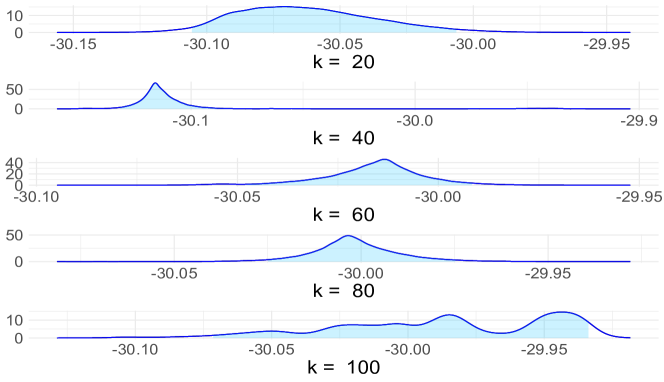
Figure 1: Posterior distribution $\hat{\Pi}_{N}$ for Example 1. The dark blue curve is the density function and the light blue area represents the $95\%$ credible interval.

Remark 3.

Let us mention that the posterior distribution $\widehat{\Pi}_{N}$ is a valid probability measure, meaning that $\widehat{\Pi}_{N}(\Theta\mid\mathcal{X}_{N})=1$. By the definition at display (2), it suffices to show the denominator, $\int e^{-N\widehat{L}(\theta)}\pi(\theta)d\theta$, is finite. Indeed, note that $\widehat{L}(\theta)>\widehat{L}(\widetilde{\theta}_{N})$ for all $\theta$ where $\widetilde{\theta}_{N}=\mathop{\mathrm{missing}}{argmin}_{\theta\in\Theta}\widehat{L}(\theta)$, hence

$$\int e^{-N\widehat{L}(\theta)}\pi(\theta)d\theta\leq e^{-N\widehat{L}(\widetilde{\theta}_{N})}\int_{\Theta}\pi(\theta)d\theta.$$

Therefore, a sufficient condition for $\int_{\Theta}e^{-N\widehat{L}(\theta)}\pi(\theta)d\theta$ being finite is $\widehat{L}(\widetilde{\theta}_{N})>-\infty$ a.s. This is guaranteed by the fact that under mild regularity assumptions, for any $\theta\in\Theta$, $\ell(\theta,x)=-\log p_{\theta}(x)>-\infty$, $P_{\theta_{0}}$ - almost surely.

2 Main results.

We are ready to state the main theoretical results for the robust posterior distribution $\widehat{\Pi}_{N}(\cdot\mid\mathcal{X}_{N})$. First, we will state them in a way that avoids technical assumptions which can be found in the latter part of the section. Recall that $L(\theta)=\mathbb{E}\ell(\theta,X)$ where $\ell(\theta,x)=-\log p_{\theta}(x)$, and let $\sigma(\Theta):=\sup_{\theta\in\Theta}\ \mbox{\rm\bf\sf var}\ \left(\ell(\theta,X)\right)$ and $\widetilde{\Delta}=\max\left(\Delta_{n},\sigma(\Theta)\right)$. The following theorem characterizes robustness properties of the mode of the posterior $\widehat{\Pi}_{N}(\cdot\mid\mathcal{X}_{N})$ defined as

$$\widehat{\theta}_{N}=\mathop{\mathrm{missing}}{argmin}_{\theta\in\Theta}\widehat{L}(\theta)-\frac{1}{N}\log\pi(\theta).$$ (5)

Theorem 1.

Under the appropriate regularity conditions on the function $\rho$, prior $\Pi$ and the family $\{p_{\theta},\ \theta\in\Theta\}$, with probability at least $99\%$,

$$\left\lvert\widehat{\theta}_{N}-\theta_{0}\right\rvert^{2}\leq C\left(\widetilde{\Delta}\left(\frac{\mathcal{O}+1}{k\sqrt{n}}+\sqrt{\frac{k}{N}}o(1)\right)\right)+O\left(\frac{1}{\sqrt{N}}\right)$$

as long as $\mathcal{O}\leq ck$ for some absolute constants $c,C>0$. Here, $o(1)$ is a function that converges to $0$ as $n\to\infty$.

In particular, stated inequality implies that as long as the number of blocks containing outliers, whose cardinality is $\mathcal{O}$, is not too large, the effect of these outliers on the squared estimation error is limited, regardless of their nature and magnitude. While the fact that the mode of $\widehat{\Pi}_{N}$ is a robust estimator of $\theta_{0}$ is encouraging, one has to address the ability of the method to quantify uncertainty to fully justify the title of the “posterior distribution.” This is exactly the content of the following result. Let $\widetilde{\theta}_{N}=\mathop{\mathrm{missing}}{argmin}_{\theta\in\Theta}\widehat{L}(\theta)$; it can be viewed as a mode of the posterior distribution corresponding to the uniform prior on $\Theta$.

Theorem 2.

Assume the outlier-free framework. Under appropriate regularity conditions on the prior $\Pi$ and the family $\{p_{\theta},\ \theta\in\Theta\}$,

$$\left\|\widehat{\Pi}_{N}(\cdot\mid\mathcal{X}_{N})-\mathcal{N}\left(\widetilde{\theta}_{N},\frac{1}{N}\left(I(\theta_{0})\right)^{-1}\right)\right\|_{TV}\overset{P}{\longrightarrow}0.$$

Moreover, $\sqrt{N}\left(\widetilde{\theta}_{N}-\theta_{0}\right)\overset{d}{\longrightarrow}\mathcal{N}\left(0,I^{-1}(\theta)\right)$.

The message of this result is that in the ideal, outlier-free scenario, the robust posterior distribution $\widehat{\Pi}_{N}$ asymptotically behaves like the usual posterior distribution $\Pi_{N}$, and that the credible sets associated with it are asymptotically valid confidence intervals. Technical requirements include a condition on the growth of the number of blocks of data, namely $k=o(n^{\tau})$ for some $\tau\in(0,1]$ defined below. The main novelty here is the first, “BvM part” of the theorem, while asymptotic normality of $\widetilde{\theta}_{N}$ has been previously established by Minsker (2020).

We finish this section by listing and discussing the complete list of regularity conditions that are required for the stated results to hold. The norm $\|\cdot\|$ refers to the standard Euclidean norm everywhere below.

Assumption 1.

The function $\rho:\mathbb{R}\mapsto\mathbb{R}_{+}$ is convex, even, and such that

1. $\rho^{\prime}(z)=z$ for $|z|\leq 1$ and $\rho^{\prime}(z)=\mathrm{const}$ for $|z|\geq 2$.

2. $z-\rho^{\prime}(z)$ is nondecreasing on $R_{+}$;

3. $\rho^{(5)}$ is bounded and Lipschitz continuous.

One example of such $\rho$ is the smoothed Huber’s loss: let

$$H(z)=\frac{z^{2}}{2}\mathbb{I}\left\{|z|\leq 3/2\right\}+\frac{3}{2}\left(|z|-\frac{3}{4}\right)\mathbb{I}\left\{|z|>3/2\right\}\,.$$

Moreover, set $\psi(z)=Ce^{-\frac{4}{1-4z^{2}}}\mathbb{I}\left\{|z|\leq\frac{1}{2}\right\}$. Then $\rho(z)=(H\star\psi)(z)$, where $\star$ denotes the convolution, satisfies assumption 1. Condition (iii) on the higher-order derivatives is technical in nature and can likely be avoided at least in some examples; in numerical simulations, we did not notice the difference between results based on the usual Huber’s loss and its smooth version. Next assumption is a standard requirement related to the local convexity of the loss function $L(\theta)$ at its global minimum $\theta_{0}$.

Assumption 2.

The Hessian $\partial^{2}_{\theta}L(\theta_{0})$ exists and is strictly positive definite.

In particular, this assumption ensures that in a sufficiently small neighborhood of $\theta_{0}$, $c(\theta_{0})\|\theta-\theta_{0}\|^{2}\leq L(\theta)-L(\theta_{0})\leq C(\theta_{0})\|\theta-\theta_{0}\|^{2}$ for some constants $0<c(\theta_{0})\leq C(\theta_{0})<\infty$. The following two conditions allow one to control the “complexity” of the class $\{\ell(\theta,\cdot),\ \theta\in\Theta\}$.

Assumption 3.

For every $\theta\in\Theta$, the map $\theta^{\prime}\mapsto\ell(\theta^{\prime},x)$ is differentiable at $\theta$ for $P$-almost all $x$ (where the exceptional set of measure $0$ can depend on $\theta$), with derivative $\partial_{\theta}\ell(\theta,x)$. Moreover, $\forall\theta\in\Theta$, the envelope function $\mathcal{V}(x\mathchar 24635\relax\;\delta):=\sup_{\|\theta^{\prime}-\theta\|\leq\delta}\left\|\partial_{\theta}\ell(\theta^{\prime},x)\right\|$ of the class $\left\{\partial_{\theta}\ell(\theta^{\prime},\cdot):\|\theta^{\prime}-\theta\|\leq\delta\right\}$ satisfies $\mathbb{E}\mathcal{V}^{2+\tau}(X\mathchar 24635\relax\;\delta)<\infty$ for some $\tau\in(0,1]$ and a sufficiently small $\delta=\delta(\theta)$.

An immediate implication of this assumption is the fact that the function $\theta\mapsto\ell(\theta,x)$ is locally Lipschitz. It other words, for any $\theta\in\Theta$, there exists a ball $B(\theta,r(\theta))$ of radius $r(\theta)$ such that for all $\theta^{\prime},\,\theta^{\prime\prime}\in B(\theta,r(\theta))$ $\lvert\ell(\theta^{\prime},x)-\ell(\theta^{\prime\prime},x)\rvert\leq\mathcal{V}(x\mathchar 24635\relax\;\delta)\|\theta^{\prime}-\theta^{\prime\prime}\|$. In particular, this condition suffices to prove consistency of the estimator $\widetilde{\theta}_{N}$.

The following condition is related to the modulus of continuity of the empirical process indexed by the gradients $\partial_{\theta}\ell(\theta,x)$. It is similar to the typical assumptions required for the asymptotic normality of the MLE, such as Theorem 5.23 in the book by Van der Vaart (2000). Define

$$\omega_{N}(\delta)=\mathbb{E}\sup_{\|\theta-\theta_{0}\|\leq\delta}\left\|\sqrt{N}\left(P_{N}-P\right)(\partial_{\theta}\ell(\theta,\cdot)-\partial_{\theta}\ell(\theta_{0},\cdot))\right\|\,,$$

where $P_{N}$ is the empirical distribution by $\tilde{\mathcal{X}}_{N}$.

Assumption 4.

The following relation holds:

$$\lim\limits_{\delta\to 0}\limsup_{N\to\infty}\omega_{N}(\delta)=0.$$

Moreover, the number of blocks $k$ satisfies $k=o(n^{\tau})$ as $k,n\to\infty$.

Limitation on the growth of $k$ is needed to ensure that the bias of the estimator $\widetilde{\theta}_{N}$ is of order $o\left(N^{-1/2}\right)$, a fact that we rely on in the proof of Theorem 2. Finally, we state a mild requirement imposed on the prior distribution; it is only slightly more restrictive than its counterpart in the classical BvM theorem (for example, Theorem 10.1 in the book by Van der Vaart (2000)).

Assumption 5.

The density $\pi$ of the prior distribution $\Pi$ is positive and bounded on $\Theta$, and is continuous on the set $\{\theta:\|\theta-\theta_{0}\|<c_{\pi}\}$ for some positive constant $c_{\pi}$.

Remark 4.

Most commonly used families of distributions satisfy assumptions 2-4. For example, this is easy to check for the normal, Laplace or Poisson families in the location model where $p_{\theta}(x)=f(x-\theta),\ \theta\in\Theta$. Other examples covered by our assumptions include the linear regression with Gaussian or Laplace-distributed noise. The main work is usually required to verify assumption 4; it relies on the standard tools for the bounds on empirical processes for classes that are Lipschitz in parameter or have finite Vapnik-Chervonenkis dimension. Examples can be found in the books by Van der Vaart (2000) and Van Der Vaart et al (1996).

3 Numerical examples and applications.

We will illustrate our theoretical findings by presenting numerical examples below. The loss function that we use is Huber’s loss defined before. While, strictly speaking, it does not satisfy the smoothness requirements, we found that it did not make a difference in our simulations. Algorithm for sampling from the posterior distributions was based on the “No-U-Turn sampler” variant of Hamiltonian Monte Carlo method (Hoffman and Gelman, 2014). Robust estimator of the log-likelihood $\widehat{L}(\theta)$ are approximated via the gradient descent algorithm at every $\theta$. Our first example demonstrates that using Huber’s loss in the framework of Example 1 is enough for BvM theorem to hold.

Example 2.

We consider two scenarios: in the first one, the data are $N=1000$ i.i.d. copies of $\mathcal{N}(-30,1)$ random variables. In the second scenario, data are generated in the same way except that $40$ randomly chosen observations are replaced with $40$ i.i.d. copies of $\mathcal{N}(10^{4},1)$ distributed random variables. Results are presented in figures 3 and 3, where the usual posterior distribution is plotted as well for comparison purposes. The main takeaway from this simple example is that the proposed method behaves as expected: as long as the number of blocks $k$ is large enough, robust posterior distribution concentrates most of its “mass” near the true value of the unknown parameter, while the usual posterior distribution is negatively affected by the outliers. At the same time, in the outlier-free regime, both posteriors perform similarly.

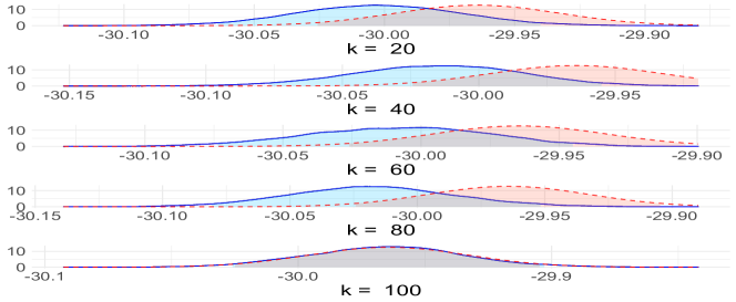
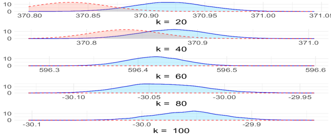
Figure 2: Posterior distribution $\hat{\Pi}_{N}$ for Example 2, scenario 1. The blue curves and blue shaded regions correspond to the density function and $95\%$ credible sets of $\hat{\Pi}_{N}$ whereas dashed red curves and red shaded region are the standard posterior and its corresponding $95\%$ credible set.

Figure 3: Posterior distribution $\hat{\Pi}_{N}$ for Example 2, scenario 2.

Example 3.

In this example, we consider a non-synthetic dataset in the linear regression framework. The dataset in question was provided by Cortez et al (2009) and describes the qualities of different samples of red and white wine. It contains $11$ “subjective” features such as fixed acidity, pH, alcohol, etc., and one “objective” feature, the scoring of wine quality; $4898$ white wine samples are selected to perform the linear regression where the objective feature is the response and the subjective features are the regressors. It is assumed that the data is sampled from the model

$$Y=\beta_{0}+\beta_{1}X_{1}+\beta_{2}X_{2}+\ldots\beta_{8}X_{8}+\varepsilon\,,$$

where $\beta_{0}$ is the intercept, $Y$ is the response, $X_{1},X_{2},\ldots,X_{8}$ are the chosen regressors (see detailed variable names in Table 1) along with the corresponding coefficients $\beta_{1},\beta_{2},\ldots,\beta_{8}$, and $\varepsilon$ is the random error with $N(0,\sigma^{2})$ distribution. Here we remark that, for simplicity only $8$ out of $11$ “subjective” features are selected such that this model agrees with the OLS linear regression model generated by best subset selection with minimization of BIC. In the second experiment, $10$ randomly chosen response variables are replaced with $\mathcal{N}(1000,10)$ random outliers. In both cases, the priors for $\beta_{j}$ are set to be $N(0,10^{2})$ for every $j$, and the prior for $\sigma$ is the uniform distribution on $(0,1]$. The block size $n$ is set to be $158$ and the number of blocks $k$ is $31$. The MAP estimates of $\beta_{j}$’s and $\sigma$, as well as the two end points of the $95\%$ credible intervals are reported in Table 1. These plots yet again demonstrate that the posterior $\widehat{\Pi}_{N}$, unlike its standard version, shows stable behavior when the input data are corrupted.

Table 1: MAP estimates of the intercept, regression coefficients and the standard deviation $\sigma$, left and right end points of $95\%$ credible intervals in parentheses.

variable name	$\widehat{\Pi}_{N}$
intercept	$-0.002(-0.026,0.022)$
fixed.acidity	$0.065(0.027,0.101)$
volatile.acidity	$-0.207(-0.232,-0.183)$
residual.sugar	$0.453(0.381,0.536)$
free.sulfur.dioxide	$0.077(0.051,0.102)$
density	$-0.487(-0.600,-0.372)$
pH	$0.125(0.093,0.160)$
sulphates	$0.075(0.049,0.101)$
alcohol	$0.287(0.227,0.350)$
$\sigma$	$0.852(0.835,0.868)$

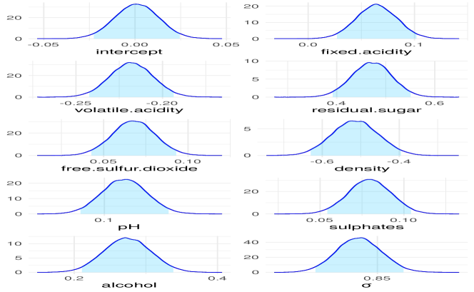
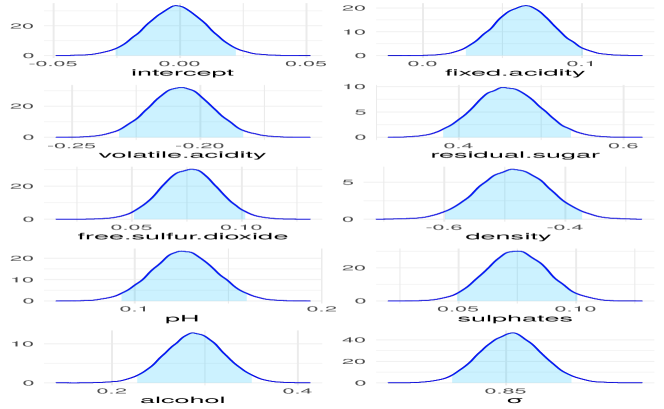
Figure 4: Posterior distribution $\widehat{\Pi}_{N}$ for Example 3, no outliers.

Figure 5: Posterior distribution $\widehat{\Pi}_{N}$ for Example 3, with outliers.

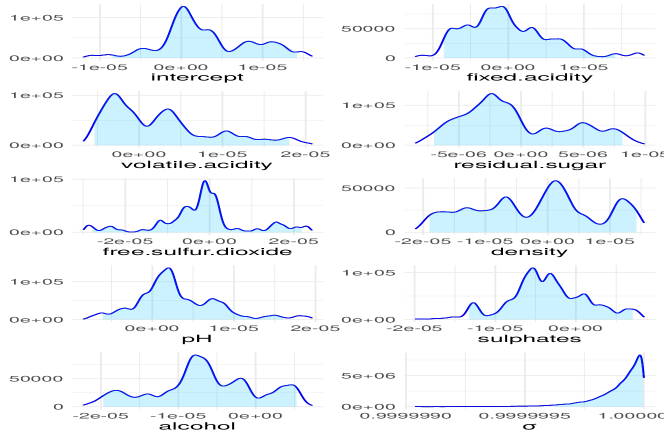
Figure 6: Standard posterior distribution for Example 3, with outliers.

4 Discussion.

The proposed extension of the median of means principle to Bayesian inference yields a version of the posterior distribution possessing several desirable characteristics, such as (a) robustness, (b) valid asymptotic coverage and (c) computational tractability. In addition, the mode of this posterior distribution serves as a robust alternative to the maximum likelihood estimator. The computational cost of our method is higher compared to the usual posterior distribution as we need to solve a one-dimensional convex optimization problem to estimate the expected log-likelihood, however, the method is still practical and, unlike many existing alternatives with similar theoretical properties, can be implemented with many off the shelf sampling packages. As with many MOM-based methods, the main “tuning parameter” is the number of blocks $k$: while larger $k$ increases robustness, smaller values $k$ reduce the bias in the estimation of the likelihood. In many examples however, this bias is far from the worst case scenario, and we observed that in our simulations, the method behaves well even when the size of each “block” is small. As a practical rule of a thumb, we recommend setting $k\asymp\sqrt{N}$ if no prior information about the number of outliers is available.

Now, let us discuss the drawbacks. First of all, the requirement for $\Theta$ to be compact is quite restrictive, and is typically necessary to ensure that the quantity $\sigma(\Theta)=\sup_{\theta\in\Theta}\ \mbox{\rm\bf\sf var}\ \left(\ell(\theta,X)\right)$ appearing in our bounds is finite. This root of this requirement is related to the fact that $\widehat{L}(\theta)$, viewed as an estimator of the mean, is not scale-invariant. At the same time, compactness assumption is satisfied if one has access to some preliminary, “low-resolution” proxy $\tilde{\theta}$ of $\theta_{0}$ such that $\|\theta_{0}-\tilde{\theta}\|\leq R$ for some, possibly large, $R>0$. Second, our method is currently tailored only for the case of i.i.d. data and the parametric models, which is the most natural setup that is natural for demonstrating the “proof of concept.” At the same time, it would be interesting to obtain practical and theoretically sound extensions that are applicable in more challenging frameworks.

5 Proofs.

This section explains the key steps behind the proofs of our mains results. The complete argument leading to Theorem 2 is rather long and technical. Here, we will outline the main ideas of the proof and the reduction steps that are needed to transform the problem into an easier one, while the missing details are included in the supplementary material.

6 Proof of Theorem 1.

In view of assumption 2, $\|\theta-\theta_{0}\|^{2}\leq c^{\prime}(\theta_{0})\left(L(\theta)-L(\theta_{0})\right)$ whenever $\|\theta-\theta_{0}\|$ is sufficiently small. Hence, if we show that $\widehat{\theta}_{N}$ satisfies this requirement, we would only need to estimate $L(\widehat{\theta}_{N})-L(\theta_{0})$. To this end, denote $L(\theta,\theta^{\prime})=L(\theta)-L(\theta^{\prime})$, and observe that

$$L(\widehat{\theta}_{N},\theta^{\prime})=L(\widehat{\theta}_{N},\theta^{\prime})-\widehat{L}(\widehat{\theta}_{N})+\widehat{L}(\widehat{\theta}_{N})+\frac{1}{N}\log(1/\pi(\widehat{\theta}_{N}))-\frac{1}{N}\log(1/\pi(\widehat{\theta}_{N}))\\ \leq L(\widehat{\theta}_{N},\theta^{\prime})-\widehat{L}(\widehat{\theta}_{N})+\widehat{L}(\theta_{0})+\frac{1}{N}\log\left(\frac{\pi(\widehat{\theta}_{N})}{\pi(\theta_{0})}\right)\\ \leq L(\theta_{0},\theta^{\prime})+2\sup_{\theta\in\Theta}\left\lvert L(\theta,\theta^{\prime})-\widehat{L}(\theta)\right\rvert+\frac{1}{N}\log\left(\frac{\pi(\widehat{\theta}_{N})}{\pi(\theta_{0})}\right).$$

If $\pi(\widehat{\theta}_{N})\leq\pi(\theta_{0})$, the last term above can be dropped without changing the inequality. On the other hand, $\pi(\theta)$ is bounded and $\pi(\theta_{0})>0$, $\frac{\pi(\widehat{\theta}_{N})}{\pi(\theta_{0})}\leq\frac{\|\pi\|_{\infty}}{\pi(\theta_{0})}$, whence the last term is at most $\frac{C(\pi,\theta_{0})}{N}$. Given $\varepsilon>0$, assumption 2 implies that there exists $\delta>0$ such that $\inf_{\|\theta-\theta_{0}\|\geq\varepsilon}L(\theta)>L(\theta_{0})+\delta$. Let $N$ be large enough so that $\frac{C(\pi,\theta_{0})}{N}\leq\delta/2$, whence $\mathbb{P}{\left(\|\widehat{\theta}_{N}-\theta_{0}\|\geq\varepsilon\right)}\leq\mathbb{P}{\left(\sup_{\theta\in\Theta}\lvert\widehat{L}(\theta)-L(\theta,\theta^{\prime})\rvert>\delta/2\right)}$. It follows from Lemma 2 in Minsker (2020) (see also Theorem 3.1 in Minsker (2018)) that under the stated assumptions,

$$\sup_{\theta\in\Theta}\left\lvert\widehat{L}(\theta)-L(\theta,\theta^{\prime})\right\rvert\leq o(1)+C\widetilde{\Delta}\frac{\mathcal{O}}{k\sqrt{n}}$$

with probability at least $99\%$ as long as $n,k$ are large enough and $\mathcal{O}/k$ is sufficiently small. Here, $o(1)$ is a function that tends to $0$ as $n\to\infty$. This shows consistency of $\widehat{\theta}_{N}$. Next, we will provide the required explicit upper bound on $\|\widehat{\theta}_{N}-\theta_{0}\|$. As we’ve demonstrated above, it suffices to find an upper bound for $L(\widehat{\theta}_{N})-L(\theta_{0},\theta^{\prime})$. We will apply the result of Theorem 2.1 in Mathieu and Minsker (2021) to deduce that for $C$ large enough, $L(\widehat{\theta}_{N})-L(\theta_{0})\leq C\left(\widetilde{\Delta}\left(\frac{\mathcal{O}+1}{k\sqrt{n}}+\sqrt{\frac{k}{N}}o(1)\right)\right)+O\left(\frac{1}{\sqrt{N}}\right)$ with probability at least $99\%$. To see this, it suffices to notice that in view of Lemma 6 in the supplementary material, $\mathbb{E}\sup_{\theta\in\Theta}\left\lvert\frac{1}{N}\sum_{j=1}^{N}\ell(\theta,X_{j})-\ell(\theta^{\prime},X_{j})-L(\theta,\theta^{\prime})\right\rvert\leq\frac{C}{\sqrt{N}}$ where $C$ may depend on $\Theta$ and the class $\{p_{\theta},\ \theta\in\Theta\}$.

6.1 Proof of Theorem 2 (sketch).

The high-level idea of the proof is fairly standard and consists in obtaining a proper (quadratic) local approximation of $\widehat{L}(\theta)$ in the neighborhood of $\theta_{0}$, coupled with careful control of the remainder terms. However, the difficulty that one has to overcome is the fact that, unlike the empirical log-likelihood, the robust estimator $\widehat{L}(\theta)$ is not linear in $-\log p_{\theta}(X)$. To do so, we develop the technical tools that are based on the existing results in the papers by Minsker (2020, 2018).

In view of the well-known property of the total variation distance,

$${\left\|\widehat{\Pi}_{N}-\mathcal{N}\left(\widetilde{\theta}_{N},\frac{1}{N}(\partial_{\theta}^{2}L(\theta_{0}))^{-1}\right)\right\|_{\mathrm{TV}}\\ =\frac{1}{2}\int_{\Theta}\Bigg{\lvert}\frac{\pi(\theta)e^{-N\widehat{L}(\theta)}}{\int_{\Theta}\pi(\theta^{\prime})e^{-N\widehat{L}(\theta^{\prime})}d\theta^{\prime}}-\frac{N^{d/2}\lvert\partial_{\theta}^{2}L(\theta_{0})\rvert^{1/2}}{(2\pi)^{d/2}}e^{-{\frac{1}{2}N(\theta-\widetilde{\theta}_{N})^{T}\partial_{\theta}^{2}L(\theta_{0})(\theta-\widetilde{\theta}_{N})}}\Bigg{\rvert}d\theta.}$$

Next, let us introduce the new variable $h=\sqrt{N}(\theta-\theta_{0})$, multiply the numerator and the denominator on the posterior by $N\widehat{L}(\theta_{0})$, and set

$${\kappa_{N}(h)=-N(\widehat{L}(\theta_{0}+h/\sqrt{N})-\widehat{L}(\theta_{0}))\\ -\frac{N}{2}(\partial_{\theta}\widehat{L}(\theta_{0}))^{T}(\partial_{\theta}^{2}L(\theta_{0}))^{-1}\partial_{\theta}\widehat{L}(\theta_{0}),}$$ (6)

and $K_{N}=\int_{\mathbb{R}^{d}}\pi(\theta_{0}+h/\sqrt{N})e^{\kappa_{N}(h)}d\mu(h)$. The total variation distance can then be equivalently written as $\left\|\hat{\Pi}_{N}-\mathcal{N}\left(\widetilde{\theta}_{N}\,,\frac{1}{N}(\partial_{\theta}^{2}L(\theta_{0}))^{-1}\right)\right\|_{\mathrm{TV}}=\frac{1}{2}\int\Big{\lvert}\frac{\pi(\theta_{0}+h/\sqrt{N})e^{\kappa_{N}(h)}}{K_{N}}-\frac{\lvert\partial_{\theta}^{2}L(\theta_{0})\rvert^{1/2}}{(2\pi)^{d/2}}e^{-{\frac{1}{2}(h-\sqrt{N}(\widetilde{\theta}_{N}-\theta_{0}))^{T}\partial_{\theta}^{2}L(\theta_{0})(h-\sqrt{N}(\widetilde{\theta}_{N}-\theta_{0}))}}\Big{\rvert}dh$. The function $\pi(\theta_{0}+h/\sqrt{N})e^{\kappa_{N}(h)}/K_{N}$ can be viewed a pdf of a new probability measure $\hat{\Pi}_{N}^{\prime}$. Thus it suffices to show that

$$\left\|\hat{\Pi}^{\prime}_{N}-\mathcal{N}\left(\sqrt{N}(\widetilde{\theta}_{N}-\theta_{0}),(\partial_{\theta}^{2}L(\theta_{0}))^{-1}\right)\right\|_{TV}\overset{P}{\longrightarrow}0\,.$$

Since $\theta_{0}$ is the unique minimizer of $L(\theta)$, $\partial_{\theta}L(\theta_{0})=0$. Next, define $H(\theta,z)=\sum_{j=1}^{k}\rho^{\prime}\left(\sqrt{n}\frac{\bar{L}_{j}(\theta)-z}{\Delta_{n}}\right)$; it is twice differentiable since both $\rho$ and $\ell$ are. It is shown in the proof of Lemma 4 in Minsker (2020) that $\partial_{z}H(\theta,\widehat{L}(\theta_{0}))\neq 0$ with high probability. Therefore, a unique mapping $\theta\mapsto\widehat{L}(\theta)$ exists around the neighborhood of $\theta_{0}$ and so do $\partial_{\theta}\widehat{L}(\theta_{0})$ and $\partial_{\theta}^{2}\widehat{L}(\theta_{0})$. Denote $Z_{N}=-(\partial^{2}_{\theta}L(\theta_{0}))^{-1}\sqrt{N}\,\partial_{\theta}\widehat{L}(\theta_{0})$. The following result, proven in the supplementary material, essentially establishes stochastic differentiability of $\widehat{L}(\theta)$ at $\theta=\theta_{0}$.

Lemma 1.

The following relation holds:

$$\sqrt{N}\left(\widetilde{\theta}_{N}-\theta_{0}\right)-Z_{N}\overset{P}{\longrightarrow}0.$$

In view of the lemma, the total variation distance between the normal laws $\mathcal{N}\left(\sqrt{N}(\widetilde{\theta}_{N}-\theta_{0}),\left(\partial^{2}_{\theta}L(\theta_{0})\right)^{-1}\right)$ and $\mathcal{N}\left(Z_{N},(\partial^{2}_{\theta}L(\theta_{0}))^{-1}\right)$ converges to $0$ in probability. Hence one only needs to show that $\left\|\hat{\Pi}^{\prime}_{N}-\mathcal{N}\left(Z_{N},(\partial^{2}_{\theta}L(\theta_{0}))^{-1}\right)\right\|_{TV}\overset{P}{\longrightarrow}0$. Let

$$\lambda_{N}(h)=-\frac{1}{2}(h-Z_{N})^{T}\partial^{2}_{\theta}L(\theta_{0})(h-Z_{N})$$ (7)

and observe that as long as one can establish that

$$\int_{\mathbb{R}^{d}}\left\lvert\pi(\theta_{0}+h/\sqrt{N})e^{\kappa_{N}(h)}-\pi(\theta_{0})e^{\lambda_{N}(h)}\right\rvert dh\overset{P}{\longrightarrow}0\,,$$ (8)

we will be able to conclude that

$${\left\lvert K_{N}-(2\pi)^{d/2}\lvert\partial^{2}_{\theta}L(\theta_{0})\rvert^{-1}\pi(\theta_{0})\right\rvert\\ =\left\lvert K_{N}-\int_{\mathbb{R}^{d}}\pi(\theta_{0})e^{\lambda_{N}(h)}d\mu(h)\right\rvert\\ \leq\int_{\mathbb{R}^{d}}\left\lvert\pi(\theta_{0}+h/\sqrt{N})e^{\kappa_{N}(h)}-\pi(\theta_{0})e^{\lambda_{N}(h)}\right\rvert dh\overset{P}{\longrightarrow}0,}$$

so that $K_{N}\overset{P}{\longrightarrow}(2\pi)^{d/2}\lvert\partial^{2}_{\theta}L(\theta_{0})\rvert^{-1}\pi(\theta_{0})$. This further implies that

$${\int_{\mathbb{R}^{d}}\left\lvert\pi(\theta_{0}+h/\sqrt{N})e^{\kappa_{N}(h)}-\frac{K_{N}\lvert\partial^{2}_{\theta}L(\theta_{0})\rvert}{(2\pi)^{d/2}}e^{\lambda_{N}(h)}\right\rvert dh\\ \leq\int_{\mathbb{R}^{d}}\left\lvert\pi(\theta_{0}+h/\sqrt{N})e^{\kappa_{N}(h)}-\pi(\theta_{0})e^{\lambda_{N}(h)}\right\rvert d\mu(h)\\ +\left\lvert\pi(\theta_{0})-\frac{K_{N}\lvert\partial^{2}_{\theta}L(\theta_{0})\rvert}{(2\pi)^{d/2}}\right\rvert\int_{\mathbb{R}^{d}}e^{\lambda_{N}(h)}dh\\ =\left\lvert\pi(\theta_{0})-\frac{K_{N}\lvert\partial^{2}_{\theta}L(\theta_{0})\rvert}{(2\pi)^{d/2}}\right\rvert\frac{(2\pi)^{d/2}}{\lvert\partial^{2}_{\theta}L(\theta_{0})\rvert}\\ +\int_{\mathbb{R}^{d}}\left\lvert\pi(\theta_{0}+h/\sqrt{N})e^{\kappa_{N}(h)}-\pi(\theta_{0})e^{\lambda_{N}(h)}\right\rvert dh\overset{P}{\longrightarrow}0,}$$

and the desired result would follow. Therefore, it suffices to establish that relation (8) holds. Moreover, since $\pi=0$ outside of a compact set $\Theta$, it is equivalent to showing that

$$\int_{\Theta^{\prime}}\left\lvert\pi(\theta_{0}+h/\sqrt{N})e^{\kappa_{N}(h)}-\pi(\theta_{0})e^{\lambda_{N}(h)}\right\rvert d\mu(h)\overset{P}{\longrightarrow}0,$$ (9)

where $\Theta^{\prime}=\{h:\theta_{0}+h/\sqrt{N}\in\Theta\}$. Note that

$$\partial_{\theta}\widehat{L}(\theta_{0}+h/\sqrt{N})-\partial_{\theta}\widehat{L}(\theta_{0})=\frac{1}{\sqrt{N}}\partial_{\theta}^{2}\widehat{L}(\theta_{0})h+o_{P}(\|h\|/\sqrt{N})\,.$$

An argument behind the proof of Lemma 1 yields (again, we present the missing details in the technical supplement) the following representation for $\kappa_{N}(h)$ defined in (6):

$$\kappa_{N}(h)=-\sqrt{N}h^{T}\partial_{\theta}\widehat{L}(\theta_{0})-\frac{1}{2}h^{T}\partial^{2}_{\theta}L(\theta_{0})h\\ -\frac{N}{2}(\partial_{\theta}\widehat{L}(\theta_{0}))^{T}(\partial_{\theta}^{2}L(\theta_{0}))^{-1}\partial_{\theta}\widehat{L}(\theta_{0})\\ -N\left(R_{1}(\theta_{0}+h/\sqrt{N})+R_{2}(\theta_{0}+h/\sqrt{N})\right)\,.$$ (10)

Let us divide $\Theta^{\prime}$ into 3 regions: $A_{N}^{1}=\{h\in\Theta^{\prime}:\|h\|\leq\|h^{0}_{N}\|\}$, $A_{N}^{2}=\{h\in\Theta^{\prime}:\|h^{0}_{N}\|<\|h\|\leq\delta\sqrt{N}\}$ and $A_{N}^{3}=\{h\in\Theta^{\prime}:\delta\sqrt{N}<\|h\|\leq R\sqrt{N}\}$ where $\delta$ is a sufficiently small positive number and $R$ is a sufficiently large so that $\{\theta\in\mathbb{R}^{d}:\|\theta-\theta_{0}\|\leq R\}$ contains $\Theta$. Finally, $h^{0}_{N}$ is chosen such that $\|h^{0}_{N}\|\rightarrow\infty$, $\|h^{0}_{N}/\sqrt{N}\|\rightarrow 0$ and that satisfies an additional growth condition specified in Lemma 8 in the supplement. The remainder of the proof is technical and is devoted to proving that each part of the integral (9) corresponding to $A_{N}^{1},\ A_{N}^{2},\ A_{N}^{3}$ converges to $0$. Details are presented in the supplementary material.

Appendix A Preliminary results.

In this section, we introduce some of the technical tools that will be used in the proofs of our main results. Lemmas 2 - 5 stated below were established in Minsker (2020), and therefore will be given without the proofs. Let $\Theta^{\prime}\subset\Theta$ be a compact set, and define

$$\tilde{\Delta}(\Theta^{\prime}):=\max(\Delta_{n},\sigma^{2}(\Theta^{\prime}))\,.$$

The following lemma provides a high probability bound for $\left\lvert\widehat{L}(\theta)-L(\theta)\right\rvert$ that holds uniformly over $\Theta^{\prime}\subset\Theta$.

Lemma 2.

Let $\mathcal{L}=\{\ell(\theta,\cdot),\ \theta\in\Theta\}$ be a class of functions mapping $S$ to $\mathbb{R}$, and assume that $\sup_{\theta\in\Theta}\mathbb{E}\left\lvert\ell(\theta,X)-L(\theta)\right\rvert^{2+\tau}<\infty$ for some $\tau\in[0,1]$. Then there exist absolute constants $c,\,C>0$ and a function $g_{\tau,P}(x)$ satisfying $g_{\tau,P}(x)\buildrel x\to\infty\over{=}\begin{cases}o(1),&\tau=0,\\ O(1),&\tau>0\end{cases}$ such that for all $s>0,$ $n$ and $k$ satisfying

$$\frac{s}{\sqrt{k}\Delta_{n}}\,\mathbb{E}\sup_{\theta\in\Theta^{\prime}}\frac{1}{\sqrt{N}}\sum_{j=1}^{N}\left\lvert\ell(\theta,X_{j}))-L(\theta)\right\rvert+g_{\tau,P}(n)\sup_{\theta\in\Theta^{\prime}}\frac{\mathbb{E}\left\lvert\ell(\theta,X)-L(\theta)\right\rvert^{2+\tau}}{\Delta_{n}^{2+\tau}n^{\tau/2}}\leq c,$$

the following inequality holds with probability at least $1-\frac{1}{s}$:

$${\sup_{\theta\in\Theta^{\prime}}\left\lvert\widehat{L}(\theta)-L(\theta)\right\rvert\leq C\Bigg{[}s\cdot\frac{\widetilde{\Delta}(\Theta^{\prime})}{\Delta_{n}}\mathbb{E}\sup_{\theta\in\Theta^{\prime}}\left\lvert\frac{1}{N}\sum_{j=1}^{N}\Big{(}\ell(\theta,X_{j})-L(\theta)\Big{)}\right\rvert\\ +\widetilde{\Delta}(\Theta^{\prime})\left(\frac{g_{\tau,P}(n)}{\sqrt{n}}\sup_{\theta\in\Theta^{\prime}}\frac{\mathbb{E}\left\lvert\ell(\theta,X)-L(\theta)\right\rvert^{2+\tau}}{\Delta_{n}^{2+\tau}n^{\tau/2}}\right)\Bigg{]}.}$$

This lemma implies that as long as $\mathbb{E}\sup_{\theta\in\Theta^{\prime}}N^{-1/2}\sum_{j=1}^{N}\left\lvert\ell(\theta,X_{j})-L(\theta)\right\rvert=O(1)$ and $\sigma^{2}(\Theta^{\prime})\lesssim\Delta_{n}=O(1)$,

$$\sup_{\theta\in\Theta^{\prime}}\left\lvert\widehat{L}(\theta)-L(\theta)\right\rvert=O_{p}(N^{-1/2}+n^{-(1+\tau)/2})\,.$$

Next, Lemma 3 below establishes consistency of the estimator $\widetilde{\theta}_{N}$ that is a necessary ingredient in the proof of the Bernstein-von Mises theorem.

Lemma 3.

$\widetilde{\theta}_{N}\rightarrow\theta_{0}$ in probability as $n,N/n\to\infty$.

The following lemma establishes the asymptotic equicontinuity of the process $\theta\mapsto\partial_{\theta}\widehat{L}(\theta)-\partial_{\theta}L(\theta)$ at $\theta_{0}$ (recall that the existence of $\partial_{\theta}\widehat{L}(\theta)$ at the neighborhood around $\theta_{0}$ has bee justified in the proof of Theorem 2).

Lemma 4.

For any $\varepsilon>0$,

$$\lim_{\delta\to 0}\limsup_{k,n\to\infty}\mathbb{P}{\left(\sup_{\|\theta-\theta_{0}\|\leq\delta}\left\|\sqrt{N}\left(\partial_{\theta}\widehat{L}(\theta)-\partial_{\theta}L(\theta)-\left(\partial_{\theta}\widehat{L}(\theta_{0})-\partial_{\theta}L(\theta_{0})\right)\right)\right\|\geq\varepsilon\right)}=0.$$

This result combined with Lemma 3 yields a useful corollary. Note that due to consistency of $\widetilde{\theta}_{N}$,

$$\partial_{\theta}L(\widetilde{\theta}_{N})-\partial_{\theta}L(\theta_{0})=\partial_{\theta}^{2}L(\theta_{0})\left(\widetilde{\theta}_{N}-\theta_{0}\right)+o_{p}\left(\left\|\widetilde{\theta}_{N}-\theta_{0}\right\|\right)\,.$$ (11)

On the other hand,

$${\partial_{\theta}L(\widetilde{\theta}_{N})-\partial_{\theta}L(\theta_{0})=\partial_{\theta}\widehat{L}(\widetilde{\theta}_{N})-\partial_{\theta}\widehat{L}(\theta_{0})\\ +\left(\partial_{\theta}L(\widetilde{\theta}_{N})-\partial_{\theta}\widehat{L}(\widetilde{\theta}_{N})\right)-\left(\partial_{\theta}L(\theta_{0})-\partial_{\theta}\widehat{L}(\theta_{0})\right)\\ =\partial_{\theta}\widehat{L}(\widetilde{\theta}_{N})-\partial_{\theta}\widehat{L}(\theta_{0})+r_{N},}$$ (12)

where $r_{N}=\left(\partial_{\theta}L(\widetilde{\theta}_{N})-\partial_{\theta}\widehat{L}(\widetilde{\theta}_{N})\right)-\left(\partial_{\theta}L(\theta_{0})-\partial_{\theta}\widehat{L}(\theta_{0})\right)$. Note that for any $\delta>0$,

$$\sqrt{N}\|r_{N}\|\leq\sqrt{N}\sup_{\|\theta-\theta_{0}\|\leq\delta}\left\|\left(\partial_{\theta}\widehat{L}(\theta)-\partial_{\theta}L(\theta)\right)-\left(\partial_{\theta}\widehat{L}(\theta_{0})-\partial_{\theta}L(\theta_{0})\right)\right\|\\ +\sqrt{N}\|r_{N}\|I\{\|\widetilde{\theta}_{N}-\theta_{0}\|>\delta\}\,.$$

The first term converges to $0$ in probability by Lemma 4 the second term converges to $0$ in probability by Lemma 3. Therefore,

$$\partial^{2}_{\theta}L(\theta_{0})\left(\widetilde{\theta}_{N}-\theta_{0}\right)+o\left(\|\widetilde{\theta}_{N}-\theta_{0}\|\right)=-\left(\partial_{\theta}\widehat{L}(\theta_{0})-\partial_{\theta}L(\theta_{0})\right)+o_{p}(N^{-1/2})\,.$$

Under assumptions of the following Lemma 5, $\sqrt{N}\left(\partial_{\theta}\widehat{L}(\theta_{0})-\partial_{\theta}L(\theta_{0})\right)$ is asymptotically (multivariate) normal, therefore, $\|\partial_{\theta}\widehat{L}(\theta_{0})-\partial_{\theta}L(\theta_{0})\|=O_{p}(N^{-1/2})$. Moreover, $\partial^{2}_{\theta}L(\theta_{0})$ is non-singular by Assumption 2. It follows that $\|\widetilde{\theta}_{N}-\theta_{0}\|=O_{p}(N^{-1/2})$, and we conclude that

$$\sqrt{N}(\widetilde{\theta}_{N}-\theta_{0})=-\left(\partial^{2}_{\theta}L(\theta_{0})\right)^{-1}\sqrt{N}\left(\partial_{\theta}\widehat{L}(\theta_{0})-\partial_{\theta}L(\theta_{0})\right)+o_{p}(1)\,.$$ (13)

Lemma 5.

The following asymptotic relations hold:

$$\sqrt{N}\left(\partial_{\theta}\widehat{L}(\theta_{0})-\partial_{\theta}L(\theta_{0})\right)\overset{d}{\longrightarrow}\mathcal{N}\left(0,I(\theta_{0})\right)\text{ and }$$

$$\sqrt{N}\left(\widetilde{\theta}_{N}-\theta_{0}\right)\overset{d}{\longrightarrow}\mathcal{N}\left(0,I^{-1}(\theta_{0})\right).$$

The following lemma demonstrates that empirical processes indexed by classes that are Lipschitz in parameter (for example, satisfying assumption 3) are “well-behaved.” This fact is well-known but we outline the proof for reader’s convenience.

Lemma 6.

Let $\mathcal{F}=\left\{f_{\theta},\ \theta\in\Theta^{\prime}\subseteq\mathbb{R}^{d}\right\}$ be a class of functions that is Lipschitz in parameter, meaning that $\lvert f_{\theta_{1}}(x)-f_{\theta_{2}}(x)\rvert\leq M(x)\|\theta_{1}-\theta_{2}\|$. Moreover, assume that $\mathbb{E}M^{2}(X)<\infty$ for some $p\geq 1$. Then

$${\mathbb{E}\sup_{\theta_{1},\theta_{2}\in\Theta^{\prime}}\frac{1}{\sqrt{n}}\left\lvert\sum_{j=1}^{n}\left(f_{\theta_{1}}(X_{j})-f_{\theta_{2}}(X_{j})-P(f_{\theta_{1}}-f_{\theta_{2}})\right)\right\rvert\\ \leq C\sqrt{d}\mathrm{diam}(\Theta^{\prime},\|\cdot\|)\mathbb{E}\|M\|_{L_{2}(\Pi_{n})}.}$$

Proof: Symmetrization inequality yields that

$$\mathbb{E}\sup_{\theta_{1},\theta_{2}\in\Theta^{\prime}}\frac{1}{\sqrt{n}}\left\lvert\sum_{j=1}^{n}\left(f_{\theta_{1}}(X_{j})-f_{\theta_{2}}(X_{j})-P(f_{\theta_{1}}-f_{\theta_{2}})\right)\right\rvert\\ \leq C\mathbb{E}\sup_{\theta_{1},\theta_{2}\in\Theta^{\prime}}\frac{1}{\sqrt{n}}\left\lvert\sum_{j=1}^{n}\varepsilon_{j}\left(f_{\theta_{1}}(X_{j})-f_{\theta_{2}}(X_{j})\right)\right\rvert\\ =C\mathbb{E}_{X}\mathbb{E}_{\varepsilon}\sup_{\theta_{1},\theta_{2}\in\Theta^{\prime}}\frac{1}{\sqrt{n}}\left\lvert\sum_{j=1}^{n}\varepsilon_{j}\left(f_{\theta_{1}}(X_{j})-f_{\theta_{2}}(X_{j})\right)\right\rvert.$$

As the process $f\mapsto\frac{1}{\sqrt{n}}\sum_{j=1}^{n}\varepsilon_{j}\left(f_{\theta_{1}}(X_{j})-f_{\theta_{2}}(X_{j})\right)$ is sub-Gaussian conditionally on $X_{1},\ldots,X_{n}$, its (conditional) $L_{p}$-norms are equivalent to $L_{1}$ norm. Hence, Dudley’s entropy bound implies that

$$\mathbb{E}_{\varepsilon}\sup_{\theta_{1},\theta_{2}\in\Theta^{\prime}}\frac{1}{\sqrt{n}}\left\lvert\sum_{j=1}^{n}\varepsilon_{j}\left(f_{\theta_{1}}(X_{j})-f_{\theta_{2}}(X_{j})\right)\right\rvert\\ \leq C\mathbb{E}_{\varepsilon}\sup_{\theta_{1},\theta_{2}\in\Theta^{\prime}}\frac{1}{\sqrt{n}}\left\lvert\sum_{j=1}^{n}\varepsilon_{j}\left(f_{\theta_{1}}(X_{j})-f_{\theta_{2}}(X_{j})\right)\right\rvert\leq C\int_{0}^{D_{n}(\Theta^{\prime})}H^{1/2}(z,T_{n},d_{n})dz,$$

where $d^{2}_{n}(f_{\theta_{1}},f_{\theta_{2}})=\frac{1}{n}\sum_{j=1}^{n}\left(f_{\theta_{1}}(X_{j})-f_{\theta_{2}}(X_{j})\right)^{2}$, $T_{n}=\left\{(f_{\theta}(X_{1}),\ldots,f_{\theta}(X_{n})),\ \theta\in\Theta^{\prime}\right\}\subseteq\mathbb{R}^{n}$ and $D_{n}(\Theta^{\prime})$ is the diameter of $\Theta$ with respect to the distance $d_{n}$. As $f_{\theta}(\cdot)$ is Lipschitz in $\theta$, we have that $d^{2}_{n}(f_{\theta_{1}},f_{\theta_{2}})\leq\frac{1}{n}\sum_{j=1}^{n}M^{2}(X_{j})\|\theta_{1}-\theta_{2}\|^{2}$, implying that $D_{n}(\Theta^{\prime})\leq\|M\|_{L_{2}(\Pi_{n})}\mathrm{diam}(\Theta^{\prime},\|\cdot\|)$ and

$$H(z,T_{n},d_{n})\leq H\left(z/\|M\|_{L_{2}(\Pi_{n})},\Theta^{\prime},\|\cdot\|\right)\leq\log\left(C\frac{\mathrm{diam}(\Theta^{\prime},\|\cdot\|)\,\|M\|_{L_{2}(\Pi_{n})}}{z}\right)^{d}.$$ (14)

Therefore,

$$\int_{0}^{D_{n}(\Theta^{\prime})}H^{1/2}(z,T_{n},d_{n})dz\leq C\sqrt{d}\mathrm{diam}(\Theta^{\prime},\|\cdot\|)\cdot\|M\|_{L_{2}(\Pi_{n})}$$

and

$$\mathbb{E}_{X}\mathbb{E}_{\varepsilon}\sup_{\theta_{1},\theta_{2}\in\Theta^{\prime}}\frac{1}{\sqrt{n}}\left\lvert\sum_{j=1}^{n}\varepsilon_{j}\left(f_{\theta_{1}}(X_{j})-f_{\theta_{2}}(X_{j})\right)\right\rvert\leq C\sqrt{d}\mathrm{diam}(\Theta^{\prime},\|\cdot\|)\mathbb{E}^{1/2}\|M\|^{2}_{L_{2}(\Pi_{n})}.$$ (15)

Next are three lemmas that we rely on in the proof of Theorem 2. Define

$$r_{N}(\theta)=\left(\partial_{\theta}L(\theta)-\partial_{\theta}\widehat{L}(\theta)\right)-\left(\partial_{\theta}L(\theta_{0})-\partial_{\theta}\widehat{L}(\theta_{0})\right).$$

Lemma 7.

For any $\theta\in\Theta$,

$$\widehat{L}(\theta)=\widehat{L}(\theta_{0})+(\theta-\theta_{0})^{T}\partial_{\theta}\widehat{L}(\theta_{0})+\frac{1}{2}(\theta-\theta_{0})^{T}\partial^{2}_{\theta}L(\theta_{0})(\theta-\theta_{0})+R_{1}(\theta)+R_{2}(\theta)\,,$$

where $R_{1}(\theta)$ and $R_{2}(\theta)$ are two functions such that for any $\theta$ satisfying $\|\theta-\theta_{0}\|\leq\delta$,

$$R_{1}(\theta)\leq\|\theta-\theta_{0}\|\sup_{\theta}\|r_{N}(\theta)\|\,,\quad\text{and}\quad\sup_{\theta}\left\lvert\frac{R_{2}(\theta)}{\|\theta-\theta_{0}\|^{2}}\right\rvert\rightarrow 0\,,$$

as $\delta\rightarrow 0$.

Let $G_{\theta}(t)=\widehat{L}\left(\theta_{0}+tv\right)$ where $v=\theta-\theta_{0}$ and note that $G^{\prime}_{\theta}(t)=v^{T}\partial_{\theta}\widehat{L}(\theta_{0}+tv)$. Then

$$\widehat{L}(\theta)=\widehat{L}(\theta_{0})+\int_{0}^{1}G^{\prime}_{\theta}(s)ds=\widehat{L}(\theta_{0})+\int_{0}^{1}G^{\prime}_{\theta}(0)ds+\int_{0}^{1}\left(G^{\prime}_{\theta}(s)-G^{\prime}_{\theta}(0)\right)ds\,.$$ (16)

The first integral equals $\partial_{\theta}\widehat{L}(\theta_{0})(\theta-\theta_{0})$. For the second integral, note that the reasoning similar to the one behind equation (11) yields that for any $\theta^{\prime}$

$$\partial_{\theta}\widehat{L}(\theta^{\prime})-\partial_{\theta}\widehat{L}(\theta_{0})-r_{N}(\theta^{\prime})=\partial_{\theta}^{2}L(\theta_{0})(\theta^{\prime}-\theta_{0})+R(\theta^{\prime}-\theta_{0})\,,$$

where $R(\theta-\theta_{0})$ is a vector-valued function such that $R(\theta-\theta_{0})/\|\theta-\theta_{0}\|\rightarrow 0$ as $\theta\rightarrow\theta_{0}$. Therefore, for any $s\in(0,1)$

$$G^{\prime}_{\theta}(s)-G^{\prime}_{\theta}(0)=v^{T}\left(\partial_{\theta}\widehat{L}(\theta_{0}+sv)-\partial_{\theta}\widehat{L}(\theta_{0})\right)\\ =s\,v^{T}\partial_{\theta}^{2}L(\theta_{0})v+v^{T}\,r_{N}(\theta_{0}+sv)+v^{T}R(sv),$$

implying that

$$\int_{0}^{1}\left(G^{\prime}_{\theta}(s)-G^{\prime}_{\theta}(0)\right)ds=\int_{0}^{1}\left(s\,v^{T}\partial_{\theta}^{2}L(\theta_{0})v+v^{T}r_{N}(\theta_{0}+sv)+v^{T}R(sv)\right)ds\\ =\frac{1}{2}v^{T}\partial_{\theta}^{2}L(\theta_{0})v+\int_{0}^{1}v^{T}r_{N}(\theta_{0}+sv)ds+\int_{0}^{1}v^{T}R(sv)ds\,.$$

Denoting the last two terms $R_{1}(\theta)$ and $R_{2}(\theta)$ respectively, and combining the previous display with equation (16), we deduce that

$$\widehat{L}(\theta)=\widehat{L}(\theta_{0})+\partial_{\theta}\widehat{L}(\theta_{0})(\theta-\theta_{0})+\frac{1}{2}(\theta-\theta_{0})^{T}\partial^{2}_{\theta}L(\theta_{0})(\theta-\theta_{0})+R_{1}(\theta)+R_{2}(\theta).$$

Moreover,

$$\int_{0}^{1}v^{T}r_{N}(\theta_{0}+sv)ds\leq\int_{0}^{1}\|v\|\sup_{t\in[0,1]}\|r_{N}(\theta_{0}+tv)\|ds=\|v\|\sup_{t\in[0,1]}\|r_{N}(\theta_{0}+tv)\|\,.$$

Therefore, for $\delta>0$ such that $\|\theta-\theta_{0}\|\leq\delta$, $R_{1}(\theta)\leq\|\theta-\theta_{0}\|\sup_{\|\theta-\theta_{0}\|\leq\delta}\|r_{N}(\theta)\|\,.$ Furthermore,

$$\int_{0}^{1}v^{T}R(sv)ds\leq\int_{0}^{1}\|v\|\sup_{t\in[0,1]}\|R(tv)\|ds=\|v\|\sup_{t\in[0,1]}\|R(tv)\|\,.$$

and

$$\frac{R_{2}(\theta_{0}+tv)}{\|v\|^{2}}\leq\frac{\sup_{t\in[0,1]}\|R(tv)\|}{\|v\|}\leq\sup_{t\in[0,1]}\left\|\frac{R(tv)}{\|tv\|}\right\|\,,$$

Thus, $\sup_{\|\theta-\theta_{0}\|\leq\delta}\left\lvert\|R_{2}(\theta)\|/\|\theta-\theta_{0}\|^{2}\right\rvert\leq\sup_{\|\theta-\theta_{0}\|\leq\delta}\left\|R(\theta-\theta_{0})\right\|/\|\theta-\theta_{0}\|$ which converges to $0$ as $\delta\rightarrow 0$.

Lemma 8.

There exits a sequence $h^{0}_{N}$ such that $\|h^{0}_{N}\|\rightarrow\infty$, $\|h^{0}_{N}/\sqrt{N}\|\rightarrow 0$ and

$$\sup_{h:\|h\|\leq\|h^{0}_{N}\|}\left\lvert N\left(R_{1}(\theta_{0}+h/\sqrt{N})+R_{2}(\theta_{0}+h/\sqrt{N})\right)\right\rvert\overset{P}{\longrightarrow}0\,,$$

where $R_{1}$ and $R_{2}$ are defined in Lemma 7.

Proof: [Proof of Lemma 8.] Let $h^{*}_{N}$ be a sequence such that $\|h^{*}_{N}\|\rightarrow\infty$ and $\|h^{*}_{N}/\sqrt{N}\|\rightarrow 0$. In view of Lemma 4,

$$\sup_{h:\|h\|\leq\|h^{*}_{N}\|}\|\sqrt{N}r_{N}(\theta_{0}+h/\sqrt{N})\|\overset{P}{\longrightarrow}0\,,$$

where $r_{N}$ is given in Lemma 7. Moreover, let $h^{(1)}_{N}$ be a sequence such that $\|h^{(1)}_{N}\|\rightarrow\infty$, $\|h^{(1)}_{N}\|\leq\|h^{*}_{N}\|$ and

$$\|h^{(1)}_{N}\|\sup_{h:\|h\|\leq\|h^{*}_{N}\|}\|\sqrt{N}r_{N}(\theta_{0}+h/\sqrt{N})\|\overset{P}{\longrightarrow}0\,.$$

Lemma 7 implies that

$$\sup_{h:\|h\|\leq\|h^{(1)}_{N}\|}\left\lvert NR_{1}(\theta_{0}+h/\sqrt{N})\right\rvert \leq\sup_{h:\|h\|\leq\|h^{(1)}_{N}\|}\left\lvert\sqrt{N}\|h\|\sup_{h:\|h\|\leq\|h^{(1)}_{N}\|}\|r_{N}(\theta_{0}+h/\sqrt{N})\|\right\rvert$$

$$\leq\|h^{1}_{N}\|\sup_{h:\|h\|\leq\|h^{(1)}_{N}\|}\|\sqrt{N}r_{N}(\theta_{0}+h/\sqrt{N})\|\overset{P}{\longrightarrow}0\,.$$

Similarly, let $h^{**}_{N}$ be a sequence such that $\|h^{**}_{N}\|\rightarrow\infty$ and $\|h^{**}_{N}/\sqrt{N}\|\rightarrow 0$. Lemma 7 yields that

$$\sup_{h:\|h\|\leq\|h^{**}_{N}\|}\left\lvert\frac{R_{2}(\theta_{0}+h/\sqrt{N})}{\|h/\sqrt{N}\|^{2}}\right\rvert\rightarrow 0\,.$$

Finally, let $h^{(2)}_{N}$ be the sequence such that $h^{(2)}_{N}\rightarrow\infty$, $\|h^{(2)}_{N}\|\leq\|h^{**}_{N}\|$ and

$$\left\|h^{(2)}_{N}\right\|^{2}\sup_{h:\|h\|\leq\|h^{**}_{N}\|}\left\lvert\frac{R_{2}(\theta_{0}+h/\sqrt{N})}{\|h/\sqrt{N}\|^{2}}\right\rvert\rightarrow 0\,.$$

Then

$$\sup_{h:\|h\|\leq\|h^{(2)}_{N}\|}\left\lvert NR_{2}(\theta_{0}+h/\sqrt{N})\right\rvert \leq\|h_{N}^{(2)}\|^{2}\sup_{h:\|h\|\leq\|h^{(2)}_{N}\|}\left\lvert\frac{R_{2}(\theta_{0}+h/\sqrt{N})}{\|h/\sqrt{N}\|^{2}}\right\rvert$$

$$\leq\|h^{(2)}_{N}\|^{2}\sup_{h:\|h\|\leq\|h^{**}_{N}\|}\left\lvert\frac{R_{2}(\theta_{0}+h/\sqrt{N})}{\|h/\sqrt{N}\|^{2}}\right\rvert\rightarrow 0\,.$$

Finally, take $h^{0}_{N}=\mathop{\mathrm{missing}}{argmin}_{h\in\{h^{(1)}_{N},h^{(2)}_{N}\}}\|h\|$, and conclude using the triangle inequality.

Lemma 9.

Let $\{U_{n}\}_{n\geq 1}$ be a sequence of random vectors that converges to $UZ$ weakly, where $Z$ is a standard random vector of dimension $d$ and $U$ is a $d\times d$ invertible matrix. Furthermore, let $V$ be a $d\times d$ symmetric positive definite matrix and $\{a_{n}\}_{n\geq 1}$ - a sequence of positive numbers converging to infinity. Then

$$\int_{\|h\|\geq a_{n}}e^{-\frac{1}{2}(h-U_{n})^{T}V(h-U_{n})}d\mu(h)\overset{P}{\longrightarrow}0\,.$$

Proof: [Proof of Lemma 9.] Note that

$$\int_{\|h\|\geq a_{n}}e^{-\frac{1}{2}(h-U_{n})^{T}V(h-U_{n})}dh\leq\int_{\|h\|\geq a_{n}}e^{-\frac{1}{2}\lambda_{\min}^{V}\|h-U_{n}\|^{2}}dh\,,$$

where $\lambda_{\min}^{V}$ is the smallest eigenvalue of $V$. Let $C$ be an arbitrary positive constant and $B_{n}=\{\|U_{n}\|\leq C\}$, then on the set $B_{n}$,

$$\int_{\|h\|\geq a_{n}}e^{-\frac{1}{2}\lambda_{\min}^{V}\|h-U_{n}\|^{2}}dh\leq\int_{\|h\|\geq a_{n}}e^{-\frac{1}{2}\lambda_{\min}^{V}(\|h\|-C)^{2}}dh\leq\delta$$

for any $\delta>0$ as $n\rightarrow\infty$. Note that $\mathbb{P}(B_{n})\rightarrow\mathbb{P}(\|UZ\|\leq C)\geq\mathbb{P}(\|Z\|^{2}\leq C(\lambda_{\min}^{U^{T}U})^{-1})$, where $\lambda_{\min}^{U^{T}U}$ is the smallest eigenvalue of $U^{T}U$. For an arbitrary $\varepsilon>0$, select $C$ such that $\mathbb{P}(\|Z\|^{2}\leq C(\lambda_{\min}^{U^{T}U})^{-1})\geq 1-\varepsilon$. Then

$$\int_{\|h\|\geq a_{n}}e^{-\frac{1}{2}(h-U_{n})^{T}V(h-U_{n})}dh\leq\delta$$

with probability at least $1-\varepsilon$, thus the assertion holds.

Appendix B Proof of Theorem 2.

We begin by filling in the details omitted in the sketch given in Section 6.1. First, Lemma 1 is implied directly by display (13) and display (10) is given by Lemma 7. For the integral over the set $A_{N}^{1}$, observe that

$$\int_{A_{N}^{1}}\left\lvert\pi(\theta_{0}+h/\sqrt{N})e^{\kappa_{N}(h)}-\pi(\theta_{0})e^{\lambda_{N}(h)}\right\rvert d\mu(h)\leq\\ \int_{A_{N}^{1}}\pi(\theta_{0}+h/\sqrt{N})\left\lvert e^{\kappa_{N}(h)}-e^{\lambda_{N}(h)}\right\rvert d\mu(h)+\int_{A_{N}^{1}}\left\lvert\pi(\theta_{0}+h/\sqrt{N})-\pi(\theta_{0})\right\rvert e^{\lambda_{N}(h)}d\mu(h)\,.$$

To estimate the first term, recall the definition of $\lambda_{N}$ in display (7) and note that

$$\lambda_{N}(h)=-\sqrt{N}h^{T}\partial_{\theta}\widehat{L}(\theta_{0})-\frac{1}{2}h^{T}\partial^{2}_{\theta}L(\theta_{0})h-\frac{N}{2}(\partial_{\theta}\widehat{L}(\theta_{0}))^{T}(\partial_{\theta}^{2}L(\theta_{0}))^{-1}\partial_{\theta}\widehat{L}(\theta_{0})\,.$$

Therefore, recalling that $\kappa_{N}$ can be written as in display (10), we have that

$$\kappa_{N}(h)=\lambda_{N}(h)-N\left(R_{1}(\theta_{0}+h/\sqrt{N})+R_{2}(\theta_{0}+h/\sqrt{N})\right),$$

hence

$$\int_{A_{N}^{1}}\pi(\theta_{0}+h/\sqrt{N})\left\lvert e^{\kappa_{N}(h)}-e^{\lambda_{N}(h)}\right\rvert dh\\ \leq\sup_{h\in A_{N}^{1}}\left\{\pi(\theta_{0}+h/\sqrt{N})\left\lvert e^{-N\left(R_{1}(\theta_{0}+h/\sqrt{N})+R_{2}(\theta_{0}+h/\sqrt{N})\right)}-1\right\rvert\right\}\int_{h\in A_{N}^{1}}e^{\lambda_{N}(h)}d\mu(h)\,.$$

Here, $\sup_{h\in A_{N}^{1}}\pi(\theta_{0}+h/\sqrt{N})\rightarrow\pi(\theta_{0})$ by the continuity of $\pi$ while

$$\sup_{h\in A_{N}^{1}}\left\lvert e^{-N\left(R_{1}(\theta_{0}+h/\sqrt{N})+R_{2}(\theta_{0}+h/\sqrt{N})\right)}-1\right\rvert\overset{P}{\longrightarrow}0\$$

by Lemma 8. Moreover, by the definition of $\lambda_{N}$ (see equation (7)), the integral factor equals $(2\pi)^{d/2}/\lvert\partial_{\theta}^{2}L(\theta_{0})\rvert$. Therefore, the first integral converges to $0$ in probability. For the second integral, observe that

$$\int_{A_{N}^{1}}\left\lvert\pi(\theta_{0}+h/\sqrt{N})-\pi(\theta_{0})\right\rvert e^{\lambda_{N}(h)}dh\\ \leq\sup_{h\in A_{N}^{1}}\left\lvert\pi(\theta_{0}+h/\sqrt{N})-\pi(\theta_{0})\right\rvert\int_{\mathbb{R}^{d}}e^{\lambda_{N}(h)}dh\\ =\sup_{h\in A_{N}^{1}}\left\lvert\pi(\theta_{0}+h/\sqrt{N})-\pi(\theta_{0})\right\rvert\frac{(2\pi)^{d/2}}{\lvert\partial_{\theta}^{2}L(\theta_{0})\rvert}\rightarrow 0\,,$$

by Assumption 5. Next, to estimate the integral over $A_{N}^{2}$, note that

$$\int_{A_{N}^{2}}\left\lvert\pi(\theta_{0}+h/\sqrt{N})e^{\kappa_{N}(h)}-\pi(\theta_{0})e^{\lambda_{N}(h)}\right\rvert dh\\ \leq\int_{A_{N}^{2}}\left\lvert\pi(\theta_{0}+h/\sqrt{N})e^{\kappa_{N}(h)}\right\rvert dh\\ +\int_{A_{N}^{2}}\left\lvert\pi(\theta_{0})e^{\lambda_{N}(h)}\right\rvert dh\,.$$

For the first term, consider again the representation of $\kappa_{N}$ as

$$\kappa_{N}(h)=-\sqrt{N}h^{T}\partial_{\theta}\widehat{L}(\theta_{0})-\frac{1}{2}h^{T}\partial^{2}_{\theta}L(\theta_{0})h-\frac{N}{2}(\partial_{\theta}\widehat{L}(\theta_{0}))^{T}(\partial_{\theta}^{2}L(\theta_{0}))^{-1}\partial_{\theta}\widehat{L}(\theta_{0})\\ -N\left(R_{1}(\theta_{0}+h/\sqrt{N})+R_{2}(\theta_{0}+h/\sqrt{N})\right)\,.$$

Since $\partial_{\theta}^{2}L(\theta_{0})$ is a positive definite matrix, $\lambda_{\min}\left(\partial_{\theta}^{2}L(\theta_{0})\right)>0$ and, in view of Lemma 7,

$$\left\lvert N\left(R_{1}(\theta_{0}+h/\sqrt{N})+R_{2}(\theta_{0}+h/\sqrt{N})\right)\right\rvert\\ \leq\|h\|^{2}\sup_{\|h\|\leq\delta\sqrt{N}}\left(\left\|\frac{\sqrt{N}r_{N}(\theta_{0}+h/\sqrt{N})}{2\|h_{0}\|}\right\|+\frac{\lvert R_{2}(\theta_{0}+h/\sqrt{N})\rvert}{\|h/\sqrt{N}\|^{2}}\right)\\ \leq\frac{\lambda_{\min}\left(\partial_{\theta}^{2}L(\theta_{0})\right)}{4}\|h\|^{2}\leq\frac{1}{4}h^{T}\partial_{\theta}^{2}L(\theta_{0})h\,,$$

with probability close to $1$, for sufficiently small $\delta$. Then

$$\kappa_{N}(h) \leq-\sqrt{N}h^{T}\partial_{\theta}\widehat{L}(\theta_{0})-\frac{1}{4}h^{T}\partial^{2}_{\theta}L(\theta_{0})h-\frac{N}{2}(\partial_{\theta}\widehat{L}(\theta_{0}))^{T}(\partial_{\theta}^{2}L(\theta_{0}))^{-1}\partial_{\theta}\widehat{L}(\theta_{0})$$

$$=-\left(h-\frac{1}{2}Z_{N}\right)^{T}\partial_{\theta}^{2}L(\theta_{0})\left(h-\frac{1}{2}Z_{N}\right)+W_{N}\,,$$

where $W_{N}=\frac{1}{2}N(\partial_{\theta}\widehat{L}(\theta_{0}))^{T}(\partial_{\theta}^{2}L(\theta_{0}))^{-1}\partial_{\theta}\widehat{L}(\theta_{0})$ and $W_{N}$ converges to $Z^{T}HZ$ weakly with $Z\sim\mathcal{N}\left(0,I_{d}\right)$ and $I_{d}$ and $H$ being a $d$-dimensional identity matrix $\frac{1}{2}I(\theta_{0})(\partial_{\theta}^{2}L(\theta_{0}))^{-1}I(\theta_{0})$ respectively. Therefore, for any positive increasing sequence $\{c_{N}\}$,

$$\int_{A_{N}^{2}}\left\lvert\pi(\theta_{0}+h/\sqrt{N})e^{\kappa_{N}(h)}\right\rvert d\mu(h)\leq\\ c_{N}\sup_{h\in A_{N}^{2}}\pi(\theta_{0}+h/\sqrt{N})\int_{h\in A_{N}^{2}}e^{-\left(h-\frac{1}{2}Z_{N}\right)^{T}\partial_{\theta}^{2}L(\theta_{0})\left(h-\frac{1}{2}Z_{N}\right)}d\mu(h)\\ +\sup_{h\in A_{N}^{2}}\pi(\theta_{0}+h/\sqrt{N})e^{W_{N}}\int_{h\in A_{N}^{2}}e^{-\left(h-\frac{1}{2}Z_{N}\right)^{T}\partial_{\theta}^{2}L(\theta_{0})\left(h-\frac{1}{2}Z_{N}\right)}d\mu(h)I\{W_{N}>\log c_{N}\}\,.$$

It is easy to see that $\sup_{h\in A_{N}^{2}}\pi(\theta_{0}+h/\sqrt{N})\int_{h\in A_{N}^{2}}e^{-\left(h-\frac{1}{2}Z_{N}\right)^{T}\partial_{\theta}^{2}L(\theta_{0})\left(h-\frac{1}{2}Z_{N}\right)}d\mu(h)$ converges to $0$ in probability by Lemma 9. Then choosing $c_{N}$ such that

$$c_{N}\sup_{h\in A_{N}^{2}}\pi(\theta_{0}+h/\sqrt{N})\int_{h\in A_{N}^{2}}e^{-\left(h-\frac{1}{2}Z_{N}\right)^{T}\partial_{\theta}^{2}L(\theta_{0})\left(h-\frac{1}{2}Z_{N}\right)}d\mu(h)\overset{P}{\longrightarrow}0\,,$$

guarantees that the first term converges to $0$. Meanwhile, the second term is $0$ with probability $\mathbb{P}\left(W_{N}\leq\log c_{N}\right)$. Note that for any $C$,

$$\mathbb{P}\left(W_{N}\leq\log c_{N}\right)=\mathbb{P}\left(W_{N}\leq\log c_{N}\right)-\mathbb{P}\left(W_{N}\leq\log C\right)\\ +\mathbb{P}\left(W_{N}\leq\log C\right)-\mathbb{P}\left(Z^{T}HZ\leq\log C\right)+\mathbb{P}\left(Z^{T}HZ\leq\log C\right)\,.$$

$\mathbb{P}\left(W_{N}\leq\log c_{N}\right)-\mathbb{P}\left(W_{N}\leq\log C\right)$ is positive for $c_{N}$ large enough by tightness and $\mathbb{P}\left(W_{N}\leq\log C\right)-\mathbb{P}\left(Z^{T}HZ\leq\log C\right)$ converges to $0$ by weak convergence. Thus, for $N$ large enough, $\mathbb{P}\left(W_{N}\leq\log c_{N}\right)\geq\mathbb{P}\left(Z^{T}HZ\leq\log C\right)$ for any $C$. Since $I(\theta_{0})$ and $\partial_{\theta}^{2}L(\theta_{0})$ are symmetric and positive definite, so is $H$. Note that for arbitrary $\varepsilon>0$, one can select a sufficiently large $C$ such that $\mathbb{P}\left(\|Z\|^{2}>\frac{\log C}{\lambda_{\max}(H)}\right)\leq\varepsilon\,.$ Therefore,

$$\mathbb{P}(Z^{T}HZ>\log C)\leq\mathbb{P}(\lambda_{\max}(H)\|Z\|^{2}>\log C)\leq\varepsilon\,.$$

Thus, for $N$ large enough,

$$\sup_{h\in A_{N}^{2}}\pi(\theta_{0}+h/\sqrt{N})e^{W_{N}}\int_{h\in A_{N}^{2}}e^{-\left(h-\frac{1}{2}Z_{N}\right)^{T}\partial_{\theta}^{2}L(\theta_{0})\left(h-\frac{1}{2}Z_{N}\right)}d\mu(h)I\{W_{N}>\log c_{N}\}$$

equals $0$ with probability at least $1-\varepsilon$ for any $\varepsilon$, hence the above term converges to $0$ in probability. We have so far shown that $\int_{A_{N}^{2}}\left\lvert\pi(\theta_{0}+h/\sqrt{N})e^{\kappa_{N}(h)}\right\rvert d\mu(h)$ converges to $0$ in probability. Another application of Lemma 9 implies that

$$\int_{A_{N}^{2}}\left\lvert\pi(\theta_{0})e^{\lambda_{N}(h)}\right\rvert d\mu(h)\leq\pi(\theta_{0})\int_{\|h\|\geq a\log N}e^{\lambda_{N}(h)}d\mu(h)\overset{P}{\longrightarrow}0\,,$$

which shows the integral over $A_{N}^{2}$ converges to $0$ in probability. For the final part, the integral over $A_{N}^{3}$, observe again that

$$\int_{A_{N}^{3}}\left\lvert\pi(\theta_{0}+h/\sqrt{N})e^{\kappa_{N}(h)}-\pi(\theta_{0})e^{\lambda_{N}(h)}\right\rvert d\mu(h)\\ \leq\int_{A_{N}^{3}}\left\lvert\pi(\theta_{0}+h/\sqrt{N})e^{\kappa_{N}(h)}\right\rvert d\mu(h)+\int_{A_{N}^{3}}\left\lvert\pi(\theta_{0})e^{\lambda_{N}(h)}\right\rvert d\mu(h)\,.$$

As before, the second integral converges to $0$ in probability by Lemma 9. The first integral can be further estimated as

$$\int_{A_{N}^{3}}\left\lvert\pi(\theta_{0}+h/\sqrt{N})e^{\kappa_{N}(h)}\right\rvert d\mu(h)\leq\int_{a\leq\|h/\sqrt{N}\|\leq R}\left\lvert\pi(\theta_{0}+h/\sqrt{N})e^{\kappa_{N}(h)}\right\rvert d\mu(h)\,.$$

On the compact set $\{\theta:\delta\leq\|\theta-\theta_{0}\|\leq R\}$, $L(\theta)-L(\theta_{0})$ attains a minimum positive value $t_{1}$. Moreover,

$$\inf_{a\leq\|h/\sqrt{N}\|\leq R}\widehat{L}(\theta_{0}+h/\sqrt{N})-\widehat{L}(\theta_{0})\geq\inf_{\|h/\sqrt{N}\|\leq R}\left(\widehat{L}(\theta_{0}+h/\sqrt{N})-L(\theta_{0}+h/\sqrt{N})\right)\\ +\inf_{a\leq\|h/\sqrt{N}\|\leq R}\left(L(\theta_{0}+h/\sqrt{N})-L(\theta_{0})\right)+\left(L(\theta_{0})-\widehat{L}(\theta_{0})\right)\,.$$

By Lemma 2, the terms in the first and third pair of brackets converge to $0$ in probability. Thus,

$$\inf_{a\leq\|h/\sqrt{N}\|\leq R}\widehat{L}(\theta_{0}+h/\sqrt{N})-\widehat{L}(\theta_{0})\geq\frac{t_{1}}{2}\,,$$

with probability approaching 1. Therefore,

$$\int_{a\leq\|h/\sqrt{N}\|\leq R}\left\lvert\pi(\theta_{0}+h/\sqrt{N})e^{\kappa_{N}(h)}\right\rvert d\mu(h)\\ \leq e^{-\frac{1}{2}Nt_{1}}\int_{\mathbb{R}^{d}}\pi(\theta_{0}+h/\sqrt{N})d\mu(h)\leq N^{d/2}e^{-\frac{1}{2}Nt_{1}}\rightarrow 0\,,$$

with probability approaching 1. This establishes the relation (8), and therefore completes the proof.

References

• \bibcommenthead
• Alon et al (1999) Alon N, Matias Y, Szegedy M (1999) The space complexity of approximating the frequency moments. Journal of Computer and system sciences 58(1):137–147
• Audibert et al (2011) Audibert JY, Catoni O, et al (2011) Robust linear least squares regression. The Annals of Statistics 39(5):2766–2794
• Baraud et al (2020) Baraud Y, Birgé L, et al (2020) Robust Bayes-like estimation: Rho-Bayes estimation. Annals of Statistics 48(6):3699–3720
• Bayarri and Berger (1994) Bayarri MJ, Berger JO (1994) Robust Bayesian bounds for outlier detection. Recent Advances in Statistics and Probability pp 175–190
• Bhattacharya et al (2019) Bhattacharya A, Pati D, Yang Y (2019) Bayesian fractional posteriors. The Annals of Statistics 47(1):39–66
• Bissiri et al (2016) Bissiri PG, Holmes CC, Walker SG (2016) A general framework for updating belief distributions. Journal of the Royal Statistical Society: Series B (Statistical Methodology) 78(5):1103–1130
• Brownlees et al (2015) Brownlees C, Joly E, Lugosi G (2015) Empirical risk minimization for heavy-tailed losses. Annals of Statistics 43(6):2507–2536
• Cortez et al (2009) Cortez P, Cerdeira A, Almeida F, et al (2009) Modeling wine preferences by data mining from physicochemical properties. Decision support systems 47(4):547–553
• Diakonikolas and Kane (2019) Diakonikolas I, Kane DM (2019) Recent advances in algorithmic high-dimensional robust statistics. arXiv preprint arXiv:191105911
• Doksum and Lo (1990) Doksum KA, Lo AY (1990) Consistent and robust Bayes procedures for location based on partial information. The Annals of Statistics pp 443–453
• Ghosh and Basu (2016) Ghosh A, Basu A (2016) Robust Bayes estimation using the density power divergence. Annals of the Institute of Statistical Mathematics 68(2):413–437
• Hoff (2007) Hoff PD (2007) Extending the rank likelihood for semiparametric copula estimation. The Annals of Applied Statistics pp 265–283
• Hoffman and Gelman (2014) Hoffman MD, Gelman A (2014) The No-U-Turn sampler: adaptively setting path lengths in Hamiltonian monte carlo. J Mach Learn Res 15(1):1593–1623
• Hooker and Vidyashankar (2014) Hooker G, Vidyashankar AN (2014) Bayesian model robustness via disparities. Test 23(3):556–584
• Jerrum et al (1986) Jerrum MR, Valiant LG, Vazirani VV (1986) Random generation of combinatorial structures from a uniform distribution. Theoretical computer science 43:169–188
• Jewson et al (2018) Jewson J, Smith JQ, Holmes C (2018) Principles of Bayesian inference using general divergence criteria. Entropy 20(6):442
• Knoblauch et al (2019) Knoblauch J, Jewson J, Damoulas T (2019) Generalized variational inference: Three arguments for deriving new posteriors. arXiv preprint arXiv:190402063
• Lecué and Lerasle (2020) Lecué G, Lerasle M (2020) Robust machine learning by median-of-means: theory and practice. Annals of Statistics 48(2):906–931
• Lerasle and Oliveira (2011) Lerasle M, Oliveira RI (2011) Robust empirical mean estimators. arXiv preprint arXiv:11123914
• Lugosi and Mendelson (2019a) Lugosi G, Mendelson S (2019a) Mean estimation and regression under heavy-tailed distributions: A survey. Foundations of Computational Mathematics 19(5):1145–1190
• Lugosi and Mendelson (2019b) Lugosi G, Mendelson S (2019b) Risk minimization by median-of-means tournaments. Journal of the European Mathematical Society 22(3):925–965
• Mathieu and Minsker (2021) Mathieu T, Minsker S (2021) Excess risk bounds in robust empirical risk minimization. Information and Inference: A Journal of the IMA
• Matsubara et al (2021) Matsubara T, Knoblauch J, Briol FX, et al (2021) Robust generalised Bayesian inference for intractable likelihoods. arXiv preprint arXiv:210407359
• Miller (2021) Miller JW (2021) Asymptotic normality, concentration, and coverage of generalized posteriors. Journal of Machine Learning Research 22(168):1–53
• Miller and Dunson (2015) Miller JW, Dunson DB (2015) Robust Bayesian inference via coarsening. arXiv preprint arXiv:150606101
• Minsker (2018) Minsker S (2018) Uniform bounds for robust mean estimators. arXiv preprint arXiv:181203523
• Minsker (2020) Minsker S (2020) Asymptotic normality of robust risk minimizers. arXiv preprint arXiv:200402328
• Nakagawa and Hashimoto (2020) Nakagawa T, Hashimoto S (2020) Robust Bayesian inference via $\gamma$-divergence. Communications in Statistics-Theory and Methods 49(2):343–360
• Nemirovsky and Yudin (1983) Nemirovsky AS, Yudin DB (1983) Problem complexity and method efficiency in optimization. Wiley-Interscience
• Svensen and Bishop (2005) Svensen M, Bishop CM (2005) Robust Bayesian mixture modelling. Neurocomputing 64:235–252
• Van der Vaart (2000) Van der Vaart AW (2000) Asymptotic statistics, vol 3. Cambridge university press
• Van Der Vaart et al (1996) Van Der Vaart AW, van der Vaart AW, van der Vaart A, et al (1996) Weak convergence and empirical processes: with applications to statistics. Springer Science & Business Media