Learning Maximum Margin Channel Decoders

Abstract

The problem of learning a channel decoder is considered for two channel models. The first model is an additive noise channel whose noise distribution is unknown and nonparametric. The learner is provided with a fixed codebook and a dataset comprised of independent samples of the noise, and is required to select a precision matrix for a nearest neighbor decoder in terms of the Mahalanobis distance. The second model is a non-linear channel with additive white Gaussian noise and unknown channel transformation. The learner is provided with a fixed codebook and a dataset comprised of independent input-output samples of the channel, and is required to select a matrix for a nearest neighbor decoder with a linear kernel. For both models, the objective of maximizing the margin of the decoder is addressed. Accordingly, for each channel model, a regularized loss minimization problem with a codebook-related regularization term and hinge-like loss function is developed, which is inspired by the support vector machine paradigm for classification problems. Expected generalization error bounds for the error probability loss function are provided for both models, under optimal choice of the regularization parameter. For the additive noise channel, a theoretical guidance for choosing the training signal-to-noise ratio is proposed based on this bound. In addition, for the non-linear channel, a high probability uniform generalization error bound is provided for the hypothesis class. For each channel, a stochastic sub-gradient descent algorithm for solving the regularized loss minimization problem is proposed, and an optimization error bound is stated. The performance of the proposed algorithms is demonstrated through several examples.

I Introduction

The success of machine learning (ML) based methods in various domains have spurred a great contemporary interest in the application of ML algorithms to communication problems [1, 2, 3, 4, 5, 6, 7, 8, 9, 10, 11, 12, 13, 14, 15]. However, state-of-the art communication systems heavily rely on expert-based design, and so obtaining a significantly improved performance with ML algorithms typically necessitates the use of the most advanced ML algorithms, most notably, deep neural networks (DNN). In accordance, this also typically prevents a theoretical justification for the developed algorithm or theoretical performance guarantees. For instance, despite a considerable effort from the statistical-learning community, the generalization properties of DNN are still considered a theoretical puzzle [16, Sec. 2].

In order to address the theoretical aspects of learning in communication systems, we take an alternative route in this paper, and focus on two basic channel models: 1) An additive noise channel model, whose noise distribution is unknown and does not even known to belong to a parametric family; and 2) A non-linear channel model with additive white Gaussian noise, whose deterministic channel transformation is unknown. Both of these models can be seen as extreme points of a general model which contains both non-linearity and additive noise from a general distribution. We focus on these two extreme cases because they represent prior knowledge on the structure of the communication problem, which is prevalent in various scenarios. More importantly, this prior knowledge leads to learning problems which are markedly different from standard classification problems in ML. Previously, in [17], empirical risk minimization (ERM) algorithms for the the additive noise channel model were considered. In this work, we focus on a different learning approach – maximum margin. Our choice of channel models and the maximum margin approach enables us to develop learning algorithms from first principles, as well as theoretical performance bounds. We thus next review the problem of learning channel decoders, and then justify the maximum margin approach.

I-A Decoder Learning

The choice of a proper channel decoder is a key element in the design of a communication system, and is typically based on rich expert knowledge. This knowledge is reflected in a statistical model of the channel operation, which then leads to optimal decoder selection and theoretical performance guarantees. The approach considered here follows the common practice of partitioning the communication epoch to a training phase – in which no data is transmitted, and the received signal is used to properly select a decoder, and a data phase – in which the decoder is fixed to its chosen value (or only tracks slight changes in the channel statistics). However, our approach here deviates from the common one to the training phase. For models with unknown noise distribution a parametric model for the noise distribution is typically assumed, the training phase is used to estimate the parameter, and an optimal decoder matched to the estimated parameter is used in the data phase. In various scenarios of interest – such as massive multiple-input multiple-output (MIMO) systems [18] or in ultra low-latency [19] communication – parameter estimation, or even the parametric modeling itself, may be inaccurate. Thus, parameter estimation during the training phase is excluded. In the same spirit, for the non-linear channel, estimation of the transformation value for each codeword may suffice. However, we target the regime in which the codebook is too large with respect to (w.r.t.) the training phase, i.e., there are not enough training samples for each codeword in order to estimate its channel-transformed value. This is similar to the common practice in linear frequency-selective channels, in which an equalizer is learned to roughly invert the channel (while accounting for noise enhancement) [20, Ch. 8 and 9].

These settings naturally motivate the use of ML methods, as they are typically distribution-free, that is, do not make any assumptions on the data statistics. In ML methods, assumptions are made, instead, on the structure of the hypothesis class. We thus follow here the typical setting in ML, in which the hypothesis class is more restricted than the true data. The choice of hypothesis class results an inductive bias and its use is then justified by its low variance, compared to richer classes of decoders. For example, a linear binary classifier can be learned even when the optimal separator between the two classes is not an hyperplane [21, Ch. 9], because it is assumed to have a proper bias-variance tradeoff. The learning process we propose, however, does not ignore the channel model, and is strongly based on both the given codebook and the structure of the channel.

For the additive noise channel, we consider the class of nearest neighbor (NN) decoders, w.r.t. the Mahalanobis distance, that are parameterized by a precision matrix. A decoder from this hypothesis class is optimal in the sense of minimizing the error probability only if the additive noise is Gaussian. The learner is provided with a fixed codebook and a dataset comprised of independent samples of the noise, and is required to select a precision matrix for a NN decoder in terms of the Mahalanobis distance. For the non-linear channel, we consider the class of NN decoders with a linear kernel, that is, decoders parameterized by a matrix. Similarly, here, a decoder based on linear kernel is optimal only if the channel transformation itself is linear. The learner is provided with a fixed codebook and a dataset comprised of independent input-output samples of the channel, and is required to select a matrix for a NN decoder with a linear kernel.

I-B Maximum Margin Learning

At first glance, the decoder learning problem is akin to multiclass classification problem, in which the class represents the index of the codeword. However these problems are different due to the prior knowledge about the channel model and the codebook. Therefore, [17] considered an ERM approach to the decoder learning problem for the additive noise channel model. However, in general, the ERM might be difficult to find, and more importantly, the ERM approach does not fully capture the structure of the codebook. For example, there could be many ERM rules which achieve zero empirical error. One of the consequences of this, is that the generalization bounds derived in [17] scale as $O(m/\sqrt{n})$, where $m$ is the number of codewords in the codebook, and $n$ is the number of noise samples provided to the learner. Therefore, in this paper we take a different approach, and derive learning rules which attempt to maximize the margin of the decoder.

The maximum margin approach is common in ML, and naturally matches the communication problem. Indeed, a NN decoder partitions the output space $\mathbb{R}^{d_{y}}$ into $m$ decision regions, where the boundaries of each such decision region (also called a Voronoi region) are $d$-dimensional hyperplanes. In the additive noise channel, this NN decoding rule maximizes the minimal Mahalanobis distance between each pair of codewords, w.r.t. the noise covariance matrix. In the non-linear Gaussian channel, the NN decoding rule maximizes the minimal Euclidean distance $d_{\text{min}}$ between each pair of transformed codewords, w.r.t. the linear kernel. As is well known, for Gaussian channels at high signal-to-noise ratio (SNR), this minimal distance is the dominant parameter in determining the error probability, or more specifically, its decay rate w.r.t. the SNR. Specifically, a union bound (over all pairs of codewords), and a Bhattacharyya-based pairwise error bound, leads to the upper bound $(m-1)\cdot\exp(-d_{\text{min}}^{2}/8\sigma^{2})$ on the error probability [22, Sec. 5.2] ($\sigma^{2}$ is the noise variance). Naturally, such a bound does not necessarily hold for non-Gaussian noise distributions. However, we adopt this criterion here for general noise distributions since in the lack of any other knowledge, maximizing the minimum distance appears to be a plausible criterion for the quality of the decoder. This approach is again common in ML. In classification, support vector machines (SVM) learn linear separating hyperplanes which aim to maximize the margin between the classes, even if the true probabilistic law results a non-linear decision boundary between the classes.

The resulting learned decoder is codebook-dependent, in the sense that it is chosen to maximize the margin, or minimal distance, between the codewords. For the non-linear channel, ideally the margin would correspond to the non-linearly transformed codewords, but as we make no assumptions on this non-linearity, the best that can be hoped for is to maximize the margin of a linear transformation of the codewords – as follows from the perspective of the assumed class of decoders.

In binary classification, the maximum margin problem is solved by transforming it to an equivalent regularized loss minimization (RLM) problem with a surrogate convex loss function, known as the hinge loss [21, Sec. 15.2]. However, in multiclass classification, the transformation from maximum margin to RLM is not immediate and requires heuristics for choosing the regularization function [23, Sec. 7], reductions to binary classification [21, Sec. 17.1], or other approximations. The maximum margin decoder learning problem studied here naturally resembles multiclass classification (when there are more than two codewords in the codebook), and accordingly, it also necessitates several steps of approximation in order to transform it to an RLM problem. Nonetheless, following these steps, the result is an RLM problem that uses a convex surrogate loss function that is specifically tailored to the decoder learning problem.

We conclude by further illuminating the difference between the decoder learning problem and standard multiclass classification. As we shall see, for the additive noise channel model, the dataset for our learning algorithm is synthesized by adding $n$ measured noise samples to each of the $m$ codewords in the codebook. This results a dataset of size $mn$, but one which has specific structure. In this synthesis of the dataset, the scaling of the codebook (henceforth referred to as “training SNR”) is a design parameter that can be chosen by the learner. One consequence of this possibility is that unlike standard classification problems, in which the margin prevailing in the dataset determines the sample complexity of the problem [21, Th. 15.4], the margin in the decoder-learning problem for the additive noise channel is a parameter to be tuned. This can be used in order to achieve the best generalization possible. Due to these differences, standard SVM learning algorithms cannot be applied, and we develop learning algorithms specifically designed for the decoder learning problem.

I-C Contributions

Our contributions and the outline of the rest of the paper are as follows. In Sec. II we establish notation conventions, formulate the learning problem for the general channel, and then specify it for the two discussed extreme special cases. In Sec. III, we formulate a maximum margin optimization problem for the decoder learning problem, and relax it in several principled steps to obtain a tractable optimization problem in the form of an RLM rule. It should be stressed, however, that the resulting optimization problem is directly designed for the decoder learning problem, and does not involve a reduction or a modification of a multiclass classification problem. In Sec. IV, we prove that the expected error probability of the learned decoder in the additive noise channel model is bounded by $m$ times the expected empirical hinge loss of the decoder plus an estimation error term of $\tilde{O}(m/(\lambda n))$, where $m$ is the number of codewords in the codebook, $\lambda$ is the regularization parameter, and $n$ is the number of available samples. Then, we constrain the precision matrix of the learned decoder to a properly chosen set and optimize the regularization parameter. The resulting generalization bound is $m$ times the optimal hinge loss plus an estimation error term of $\tilde{O}(m/\sqrt{n}))$. The proof of this generalization bound is based on establishing an on-average-replace-one-stability property. We then use this generalization bound to offer a theoretical guideline for choosing the training SNR. We then prove analogous expected generalization bounds for the non-linear channel. In addition, we prove a $O(1/\sqrt{n})$ uniform high-probability generalization error bound for the hinge-type loss function, for any decoder from the chosen decoder class for the non-linear channel.

The RLM mentioned above is tractable, yet still suffers from large complexity, mainly due to a $O(n^{2})$ dependence on the number of samples $n$, similarly to the computational cost associated with SVM problems [24]. For classification SVM, this problem was addressed in [25], which proposed a stochastic sub-gradient descent algorithm for solving the RLM problem called PEGASOS (primal estimated sub-gradient solver for SVM). In Sec. V, we develop an algorithm in that spirit for the decoder learning problem, and prove that $\tilde{O}(1/\epsilon)$ iterations suffice in order to obtain a solution of accuracy $\epsilon$. We stress that this bound does not depend on the problem’s dimension or the number of samples, which can be large in many communication problems. On top of that, each iteration of the algorithm requires low computational power, and thus suitable to learning on low-complexity devices. In Sec. VI, we exemplify the operation of the algorithm through simulation for several noise distributions, channel transformations, and codebooks. In Sec. VII, we summarize the paper and propose several directions for further research. All the proofs are deferred to the appendixes.

I-D Other Related Work

As said, the recent success of ML algorithms (most notably DNNs) in various problem domains [26] has spurred interest in applying machine-learning algorithms as a part of a communication system [1, 27]. These applications can be roughly divided to several approaches, and here we briefly mention a sample of them. One approach is to use a machine-learning algorithm as a replacement to one or more components of the system. Examples include [28] for channel equalization, [15] for channel encoder and decoder, [8, 14, 7] for channel decoder, and [29, 30, 31] for channel estimation. A second approach is to modify an existing algorithm by incorporating DNNs. In [3] DNNs are used in the belief propagation algorithm, in [6] for the Viterbi algorithm, in [32] for iterative decoding algorithms, such as bit-flipping and residual belief propagation. Among the classical ML algorithms, SVMs gained high popularity and enjoy strong theoretical guarantees. A SVM based receiver that combines the pilot-based channel estimation, data demodulation and decoding processes in one joint operation was proposed in [33]. They considered first-order Gauss-Markov fading process and additive Gaussian noise with $N$ dimensional encoding vector. The system was composed from $N$ classifiers, one per bit, or $2^{N}$ classifiers in the one-vs.-one or one-vs.-rest techniques. SVM regression (SVR) was used in [34, 35] for channel estimation. We note in passing, that similar theoretical studies have been performed for the source coding problem of learning vector quantizers [36, 37, 38, 39, 40].

Channel decoding in non-linear channels was studied earlier in [41, 42]. The non-linear channel can practically model the nonlinear effects in wireless communication systems, the Kerr non-linearity in optical fibers, and the saturation non-linearity of amplifies [43, 44]. Information theoretic limits on the capacity of non-linear fiber-optic channels were studied in [45, 46, 47], and the shaping gain in these channels was studied in [48].

II Problem Formulation

II-A Notation Conventions

Random variables or vectors are denoted by capital letters and specific values they take are denoted by the corresponding lower case letters. The expectation operator is denoted by $\mathbb{E}_{\mu}[\cdot]$ where $\mu$ is the underlying probability measure, which is omitted if understood from context. The tail function of the standard normal distribution is denoted by $Q(x)$. The indicator of an event $\mathcal{A}$ is denoted by $\mathbb{I}\{\mathcal{A}\}$. The probability simplex is denoted by $\Delta^{d}\triangleq\{v\in\mathbb{R}_{+}^{d}:\sum_{i\in\left[d\right]}v_{i}=1\}$. All vectors are taken as column vectors. The standard Euclidean norm for $x\in\mathbb{R}^{d}$ is denoted by $\lVert x\rVert$ and the inner product by either $\langle x_{1},x_{2}\rangle$ or $x_{1}^{T}x_{2}$, interchangeably. The Frobenius norm for a matrix $A\in\mathbb{R}^{d\times d}$ is denoted by $\|A\|_{F}$. The operator norm for a matrix $A\in\mathbb{R}^{d_{y}\times d_{x}}$ is denoted by $\|A\|_{\text{op}}\triangleq\sup_{v\in\mathbb{R}^{d_{x}}\colon\|v\|\leq 1}\|Av\|$. The positive semidefinite (PSD) cone is denoted by $\mathbb{S}_{+}$. The minimal (resp. maximal) eigenvalue of a symmetric matrix $A$ is denoted by $\lambda_{\text{min}}(A)$ (resp. $\lambda_{\text{max}}(A)$) . For $n\in\mathbb{N}^{+}$, the set $\{1,2,\dots,n\}$ is denoted by $[n]$. Standard Bachmann-Landau asymptotic notation will be used, where specifically, $\tilde{O}(\cdot)$ is such that the logarithmic factors are hidden, namely, $f(n)\in\tilde{O}(h(n))\iff\exists k:f(n)\in O(h(n)\log^{k}(h(n)))$.

II-B Channel Models

Consider the problem of communication over a general channel

$$Y=f(X)+Z,$$ (1)

where, $Y\in\mathbb{R}^{d_{y}}$ is the channel output, $X\in\mathbb{R}^{d_{x}}$ is a codeword that is chosen from a fixed given codebook $C=\{x_{j}\}_{j\in\left[m\right]}$ with a uniform probability, $f:\mathbb{R}^{d_{x}}\rightarrow\mathbb{R}^{d_{y}}$ is a deterministic channel transformation, and $Z\in\mathbb{R}^{d_{y}}$ is a noise statistically independent of the input $X$. The unknown channel operation (1), is denoted by $\mu$ and is thus comprised of the deterministic $f$ and the distribution of $Z$, both which are unknown to the designer of the decoder. It is further assumed that the decoder is chosen from the class of NN decoders with Mahalanobis distance and linear kernel given by

$$\hat{j}\left(y\right)\in\operatorname*{arg\,min}_{j\in\left[m\right]}\left\|Hx_{j}-y\right\|_{S}\triangleq\operatorname*{arg\,min}_{j\in\left[m\right]}\sqrt{\left(Hx_{j}-y\right)^{T}S\left(Hx_{j}-y\right)},$$ (2)

where $S\in\mathbb{S}_{+}^{d_{x}}$ is a precision matrix (the inverse of the covariance matrix) and $H\in\mathbb{R}^{d_{y}\times d_{x}}$ is a linear kernel. As well known, this class is optimal if the channel transformation is linear $f(x)=Hx$ and the noise is Gaussian with inverse covariance matrix $S$, but it is not assumed here that the channel model obeys this model.

For a decoder $(H,S)$, the expected error probability conditioned that the $j$th codeword was transmitted is given by

$$\boldsymbol{p}_{\mu}\left(H,S\mid j\right)=\mathbb{E}_{\mu}\left[\mathbb{I}\left\{\min_{j^{{}^{\prime}}\in\left[m\right]\backslash\left\{j\right\}}\left\|Hx_{j^{\prime}}-Y\right\|_{S}<\left\|Hx_{j}-Y\right\|_{S}\right\}\;\middle|\;Y=f\left(x_{j}\right)+Z\right],$$ (3)

and the expected error probability, averaged over all codewords, is given by

$$\boldsymbol{p}_{\mu}\left(H,S\right)=\frac{1}{m}\sum_{j\in\left[m\right]}\boldsymbol{p}_{\mu}\left(H,S|j\right).$$ (4)

A learner, which does not know $\mu$, is provided with $n$ input-output samples $\boldsymbol{D}=\{X_{i},Y_{i}\}_{i\in[n]}$ where $X_{i}\in C$, and $Y_{i}$ is the corresponding channel output (1) for input $X_{i}$, $i\in[n]$. Based on this dataset, and the given codebook $C$, the learner is required to find $(H,S)$ which minimize the expected error probability. A common learning approach is ERM, which aims to minimize the empirical average error probability of the noise samples, given by

$$\boldsymbol{p}_{\boldsymbol{D}}\left(H,S\right)=\frac{1}{n}\sum_{i\in[n]}\mathbb{I}\left\{\min_{x^{\prime}\in C\backslash\{x_{i}\}}\left\|Hx^{\prime}-y_{i}\right\|_{S}<\left\|Hx_{i}-y_{i}\right\|_{S}\right\}.$$ (5)

In this paper, we focus on two structured extremes of this model, which both result decoder classes which are substantially different from multiclass classifiers, and are also relevant in practical communication scenarios in which further prior knowledge on the model exists. The first one is an additive noise channel model that assumes that $f$ is the identity transformation, and the second one is a non-linear channel model that assumes that the noise is Gaussian. These models best illuminate the affect of the structure of the communication channel model on the decoder learning problem. The general model (1) is not more challenging than these two extreme models, and bounds and algorithms can be easily obtained for the general model by combining the results obtained in this paper for the two extreme models.

II-B1 The Additive Noise Channel

In the first specified channel model that we consider, the channel transformation is assumed to be the identity function, and so (1) becomes $Y=X+Z$. We thus henceforth denote for this model $d\triangleq d_{x}=d_{y}$. For this channel model, we restrict the general class (2) to have $H=I$, and this results a class of NN decoders with Mahalanobis distance, given by

$$\hat{j}\left(y\right)\in\operatorname*{arg\,min}_{j\in\left[m\right]}\left\|x_{j}-y\right\|_{S}\triangleq\operatorname*{arg\,min}_{j\in\left[m\right]}\sqrt{\left(x_{j}-y\right)^{T}S\left(x_{j}-y\right)},$$ (6)

parameterized by a precision matrix $S\in\mathbb{S}_{+}^{d}$. In what follows, we will identify a decoder from this class by its precision matrix $S$. Since the channel law only depends on the noise distribution, learning the noise distribution can be made with arbitrary inputs, which we take for simplicity to be $X\equiv 0$. Thus, we assume that the learner is equipped with $n$ noise samples $\boldsymbol{Z}=\{Z_{i}\}_{i\in\left[n\right]}$ drawn independent and identically distributed (i.i.d.) from the distribution of $Z$. The learner synthesize a new dataset from these noise samples comprised of $mn$ labeled samples, in which each of the scaled codewords in the codebook is perturbed by one of the noise samples $\{Z_{i}\}_{i\in[n]}$, namely

$$\boldsymbol{D}\left(\boldsymbol{Z}\right)\triangleq\left\{Y_{k},l_{k}\right\}_{k=1}^{mn}=\bigcup_{j\in\left[m\right]}\boldsymbol{D}_{j}\left(\boldsymbol{Z}\right),$$ (7)

where $\boldsymbol{D}_{j}(\boldsymbol{Z})\triangleq\{\Gamma\cdot x_{j}+Z_{i},j\}_{i\in\left[n\right]}$, and where $\Gamma>0$ is a scaling constant which determines the training SNR. We note that this dataset has $nm$ points, but it is based only on $n$ random noise samples. For the sake of brevity, we will omit from now the explicit dependence of $\boldsymbol{D}$ in $\boldsymbol{Z}$. Henceforth, we refer to this model as the additive noise channel model. A learner is then required to find $S$ which minimizes the expected error probability based on $\boldsymbol{D}$.

II-B2 The Non-linear White Gaussian Noise Channel

In the second specified channel model that we consider, the noise is assumed to be white and Gaussian, and so (1) becomes $Y=f(X)+W$, where $W\in\mathbb{R}^{d_{y}}$ is a white Gaussian noise, statistically independent of the input $X$. For this channel model, we restrict the general class (2) to have $S=I$, and this results a class of NN decoders, given by

$$\hat{j}(y)\in\operatorname*{arg\,min}_{j\in[m]}\left\|y-Hx_{j}\right\|,$$ (8)

parameterized by a linear-kernel matrix $H\in\mathcal{H}\triangleq\mathbb{R}^{d_{y}\times d_{x}}$. In what follows, we will identify a decoder from this class by its matrix $H$. We assume that the learner is equipped with $n$ input-output samples $\boldsymbol{D}=\{J_{i},Y_{i}\}_{i\in[n]}$, where $J_{i}$ is chosen i.i.d. and uniformly over $[m]$, and $Y_{i}$ is the corresponding channel output for input $X_{J_{i}}$. Henceforth, we refer to this model as the non-linear channel model. A learner is then required to find $H$ which minimizes the expected error probability based on $\boldsymbol{D}$.

The matrix $H$ serves as a linear approximation of $f(\cdot)$, which is non-linear in general. Note that knowing $f(x_{j})$ for any $x_{j}\in C$ suffices for optimal decoding, but we target the regime in which the codebook is large w.r.t. the dataset, and so there are not enough training samples for each codeword $x_{j}$ in order to accurately estimate $f(x_{j})$. In addition, although this class does not have optimality guarantees for a non-linear channel, it is possible to enrich its expressive power by first mapping the codewords into a high dimensional feature space [21, Ch. 16].

III Maximum Margin by RLM

In this section, we develop RLM problems for the decoder learning problem that are strongly connected to the original maximum margin objective. In Sec. III-A we present the corresponding RLM problem for the additive noise channel model. We then state the steps required for its development, with proofs appearing in Appendix A-A. Then, in Sec. III-B, we present the RLM problem for the non-linear channel model. The steps required for its development and the corresponding proofs both appear in Appendix A-B.

For brevity, we will henceforth denote $\delta_{pq}\triangleq x_{p}-x_{q}$ as the difference between a pair of codewords in the codebook. For notational convenience, we will henceforth also use a single index in the set $[\frac{1}{2}m(m-1)]$ to specify a pair of codewords (instead of double indices $\{(p,q)\}_{1\leq p<q\leq m}$ ). In addition, we define the following property of a partition of the codeword-pairs.

Definition 1.

A partition $P=\bigcup_{j=1}^{d+1}P_{j}$ of $\{(p,q)\}_{1\leq p<q\leq m}$ is called proper if $\operatorname{Span}[\{\delta_{p_{j},q_{j}}\}_{j=1}^{d+1}]=\mathbb{R}^{d}$ for any set of representatives $\{\delta_{p_{j},q_{j}}\}_{j=1}^{d+1}$, such that $(p_{j},q_{j})\in P_{j}$ for all $j\in[d+1]$.

The RLM problems that we will next present will use proper partitions for their regularization terms. We assume, without loss of generality (w.l.o.g.), that $\operatorname{Span}\{\delta_{pq}\}_{1\leq p<q\leq m}=\mathbb{R}^{d}$. Then, a simple way of finding a proper partition is by first finding a basis of $\mathbb{R}^{d}$: $\{\delta_{p_{j},q_{j}}\}_{j=1}^{d}\subset\{\delta_{pq}\}_{1\leq p<q\leq m}$ and then setting $P_{j}=\{\delta_{p_{j},q_{j}}\}$ for all $j\in[d]$ and $P_{d+1}=\{\delta_{pq}\}_{1\leq p<q\leq m}\setminus\{\delta_{p_{j},q_{j}}\}_{j=1}^{d}$. Nonetheless, the RLM problem (and subsequent results in what follows) holds for any arbitrary proper partition.

III-A The Additive Noise Channel RLM

The RLM problem for the additive noise channel model requires a few additional definitions, as follows. For a given ordered pair of codeword indices $(p,q)$, and a sample $y_{i}\in\boldsymbol{D}_{p}\bigcup\boldsymbol{D}_{p}$, we denote the following transformation of the sample and codewords $a_{pqi}\triangleq(-1)^{\mathbb{I}(i\in\boldsymbol{D}_{q})}(y_{i}-\frac{1}{2}(x_{p}+x_{q}))$. Then, we denote by $\mathring{\ell}^{\text{hinge}}(S,p,q,i)\triangleq\max\{0,1-a_{pqi}^{T}S\delta_{pq}\}$, a hinge-type surrogate loss function, and by

$$\mathring{L}_{\boldsymbol{D}}^{\text{hinge}}\left(S\right)\triangleq\frac{2}{m\left(m-1\right)}\sum_{1\leq p<q<m}\frac{1}{2n}\sum_{i\in\boldsymbol{D}_{p}\bigcup\boldsymbol{D}_{q}}\mathring{\ell}^{\text{hinge}}\left(S,p,q,i\right)$$ (9)

the average hinge loss of the induced binary linear classifiers $\{S\delta_{pq}\}$, over the transformed noise samples $\{a_{pqi}\}$. Let $P=\bigcup_{i=1}^{d+1}P_{i}$ be a proper partition according to Definition 1, let $\{\eta_{i}\}_{i\in\left[d+1\right]}$ be positive parameters which sum to $1$, and let $\lambda>0$ be a regularization parameter that controls the tradeoff between the loss and the regularization. We show in this section that the RLM learning rule

$$\min_{S\in\mathbb{S}_{+}}\mathring{L}_{\boldsymbol{D}}^{\text{hinge}}\left(S\right)+\lambda\sum_{i=1}^{d+1}\eta_{i}\max_{j\in P_{i}}\left\|S\delta_{j}\right\|^{2},$$ (10)

learns a precision matrix which maximizes a lower bound on the margin among all codeword-pairs.

At this point, we may compare the surrogate loss function obtained here to a different surrogate hinge-type upper bound for the average error probability loss over $\boldsymbol{Z}$ proposed in [17]. There, the hinge-type surrogate loss function was defined as

$$\bar{L}_{\boldsymbol{Z}}^{\text{hinge}}\left(S\right)\triangleq\frac{1}{n}\sum_{i\in\left[n\right]}\frac{1}{m}\sum_{p\in\left[m\right]}\max\left\{0,1-\min_{q\in\left[m\right]\backslash\left\{p\right\}}\left\|x_{p}+z_{i}-x_{q}\right\|_{S}-\left\|z_{i}\right\|_{S}\right\}.$$ (11)

The hinge loss functions (9) and (11) are rather different, and are the result of different types of relaxations. We review these differences in light of two possible ways in which the optimization problem of SVM for binary classification is typically interpreted. The first interpretation is that the SVM objective function is a convex and continuous upper bound to the non-convex and discontinuous zero-one loss function. The regularization term can be interpreted as a standard Tikhonov regularization term. The motivation of changing the zero-one loss to a hinge-type loss function is that the resulting ERM problem can be more efficiently solved compared to the ERM problem for the zero-one loss. With this interpretation, the choice of hinge loss function is arbitrary, and, in principle, any convex upper bound on the zero-one loss is also appropriate. The second interpretation of the optimization problem of SVM is in terms of margin maximization. For inseparable datasets, the objective function of SVM is interpreted as a balance between increasing the margin and increasing the classification errors. As well known, for binary classification, both interpretations lead to exactly the same optimization problem [21, Ch. 15]. This is, however, not the case for the decoder learning problem. The hinge loss function in [17] follows the first interpretation for minimizing the error probability of the channel decoder. This approach leads to an ERM problem with the hinge loss over the noise samples, and an implicit regularization in the form of maximal eigenvalue constraint. However, this hinge loss is not directly related to the margin. In this paper, we follow the second interpretation for maximizing the margin induced by the channel decoder. This approach leads to an RLM problem with the hinge loss over the transformed noise samples and a codebook related regularization in (10). Hence, unlike SVM, the two approaches lead to different optimization problems for the channel decoding problem, where the main source of difference is in fact due to the lower bound taken in step 2. We argue that for the channel decoding problem the second approach is better since error probability is strongly related to margin, as discussed above.

The development of the optimization problem (10) will be made in several steps, which we next describe in detail.

Step 1 – maximization of the minimum margin

We begin with the assumption that the dataset $\boldsymbol{D}$ is separable, i.e., there exists a precision matrix $S$ that achieves zero loss over $\boldsymbol{D}$. While this is a rather strong assumption for a general dataset, it is only a staring point which will be relaxed in the following steps. It is also analogous to the linear separability assumption made for hard SVM, which is also used as a starting point to soft SVM [21, Ch. 15]. In fact, in our setting, separability can always be achieved by setting the training-SNR parameter $\Gamma$ to be large enough. The margin of a hyperplane w.r.t. a dataset is defined to be the minimal distance between a point in the dataset and the hyperplane [21, Ch. 15]. The learner’s goal is to find a precision matrix $S$ that maximizes the minimum margin, over all codeword-pairs $x_{p},x_{q}\in C$, according to the Mahalanobis distance w.r.t. $S$. This learning problem is formulated as the following margin-maximization problem, given as follows:

Claim 2.

The maximum margin induced by a Mahalanobis distance NN decoder with precision matrix $S$ is

$$\max_{S\in\mathbb{S}_{+}}\min_{1\leq p<q\leq m}\min_{i\in\boldsymbol{D}_{p}\cup\boldsymbol{D}_{q}}\frac{a_{pqi}^{T}S\delta_{pq}}{\left\|S\delta_{pq}\right\|}.$$ (12)

Step 2 – a convex lower bound

The previous problem is not necessarily convex, and therefore we proceed to maximize the following convex lower bound on its value.

Claim 3.

The problem

$$\begin{array}[]{cc}\max_{S\in\mathbb{S}_{+}}\min_{1\leq p<q\leq m}\min_{i\in\boldsymbol{D}_{p}\cup\boldsymbol{D}_{q}}&a_{pqi}^{T}S\delta_{pq}\\ \operatorname{subject\;to}&\max_{1\leq p<q\leq m}\left\|S\delta_{pq}\right\|\leq 1\end{array}$$ (13)

is a convex optimization problem, whose value is a lower bound on the value of (12).

Step 3 – minimum norm formulation

With the prospect removal of the separability assumption, we next derive a minimum norm optimization problem, so that every solution to it is a solution to (13). This step is analogous to the equivalent formulation of hard SVM as a quadratic optimization problem [21, Ch. 15.1].

Lemma 4.

Every solution to the following minimum norm problem

$$\begin{array}[]{cc}\min_{S\in\mathbb{S}_{+}}\max_{1\leq p<q\leq m}&\left\|S\delta_{pq}\right\|^{2}\\ \operatorname{subject\;to}&\min_{1\leq p<q\leq m}\min_{i\in\boldsymbol{D}_{p}\cup\boldsymbol{D}_{q}}a_{pqi}^{T}S\delta_{pq}\geq 1\end{array},$$ (14)

is a solution to (13).

Step 4 – relaxation of the separability assumption

Next, we introduce slack variables in order to relax the assumption that the dataset $\boldsymbol{D}$ is separable. This step is analogous to the relaxation made for soft SVM [21, Ch. 15.2]. A short derivation in Appendix A-A results the RLM problem

$$\min_{S\in\mathbb{S}_{+}}\mathring{L}_{\boldsymbol{D}}^{\text{hinge}}\left(S\right)+\lambda\cdot\max_{1\leq p<q\leq m}\left\|S\delta_{pq}\right\|^{2}.$$ (15)

Step 5 – inducing stability by a generalization of the regularization

Some of the generalization bounds for SVM are based on the stability of its learning rule. However, the problem (15) is, in general, not stable, due to the fact that the regularization term $\max_{1\leq p<q\leq m}\|S\delta_{pq}\|^{2}$ is indifferent to changes in directions orthogonal to the maximizer $\delta_{pq}$. Nonetheless, we next assume, w.l.o.g., that $\operatorname{Span}\{\delta_{pq}\}_{1\leq p<q\leq m}=\mathbb{R}^{d}$, and slightly modify the learning rule to a stable one. The final RLM rule for finding a maximum minimum margin decoder is defined for given positive parameters $\{\eta_{i}\}_{i\in\left[d+1\right]}$ which satisfy $\sum_{i=1}^{d+1}\eta_{i}=1$, and a proper partition $\{P_{j}\}_{j\in\left[d+1\right]}$, as

$$A\left(\boldsymbol{D}\right)=\operatorname*{arg\,min}_{S\in\mathbb{S}_{+}}\mathring{L}_{\boldsymbol{D}}^{\text{hinge}}\left(S\right)+\lambda\sum_{i=1}^{d+1}\eta_{i}\max_{j\in P_{i}}\left\|S\delta_{j}\right\|^{2}.$$ (16)

The stability of this learning rule will be used in Sec. IV to derive generalization bounds.

III-B The Non-linear Gaussian Noise Channel RLM

The RLM problem for the non-linear Gaussian noise channel uses the following definitions. Let $K\in\mathcal{K}\triangleq\mathbb{S}_{+}^{d_{x}}$ be an auxiliary matrix variable. We denote by

$$\mathring{\ell}^{\text{hinge}}(H,K,i)\triangleq\frac{1}{m-1}\sum_{j^{\prime}\in\left[m\right]\backslash\left\{j_{i}\right\}}\max\left\{0,1-\left[y_{i}^{T}H\delta_{j_{i}j^{\prime}}-\frac{1}{2}\left(x_{j_{i}}+x_{j^{\prime}}\right)^{T}K\delta_{j_{i}j^{\prime}}\right]\right\}$$ (17)

a hinge-type surrogate loss function, and by

$$\mathring{L}_{\boldsymbol{D}}^{\text{hinge}}\left(H,K\right)\triangleq\frac{1}{n}\sum_{i\in\left[n\right]}\mathring{\ell}^{\text{hinge}}\left(H,K,i\right)$$ (18)

the average hinge loss over the dataset. As before, let $P=\bigcup_{i=1}^{d+1}P_{i}$ be a proper partition, let $\{\eta_{i}\}_{i\in\left[d+1\right]}$ be positive parameters which sum to $1$, and let $\lambda>0$ be a regularization parameter. We show in Appendix A-B that the RLM learning rule

$$\begin{array}[]{cc}\min_{\left(H,K\right)\in\mathcal{H}\times\mathcal{K}}&\mathring{L}_{\boldsymbol{D}}^{\text{hinge}}\left(H,K\right)+\lambda\sum_{i=1}^{d+1}\eta_{i}\left[\max_{j\in P_{i}}\left\|H\delta_{j}\right\|^{2}+\max_{j^{\prime}\in P_{i}}\left\|K\delta_{j^{\prime}}\right\|^{2}\right]\\ \operatorname{subject\;to}&H^{T}H\preceq K\end{array},$$ (19)

learns a linear kernel $H$ which approximately maximizes a lower bound on the margin among all codeword-pairs. The derivation is similar to the one for the additive noise channel. In what follows we will describe only the main differences, and the full derivation can be found in Appendix A-B.

The key difference between the two derivations is that while the decoder class for the additive noise channel is linear in its parameter $S$, the decoder class for the non-linear Gaussian noise channel is quadratic in its parameter $H$. The first consequence of this difference is that even after taking the lower bound in step $2$, the problem is still not necessarily convex. The second consequence of this difference is in establishing a minimum norm problem, in step 3. The technique which we use (following SVM-type analysis) is only suitable for linear classifiers. Therefore, we proceed by a linearization of the decoder, replacing $H^{T}H$ with an auxiliary PSD matrix $K\in\mathcal{K}\triangleq\mathbb{S}_{+}^{d_{x}}$. Nonetheless, we note that the learned decoder will be parameterized only by $H$. Therefore, at the next step we add a constraint that links the auxiliary matrix $K$ to $H$ as $H^{T}H=K$, and then further take a convex relaxation, namely $H^{T}H\preceq K$.

IV Generalization Error Bounds

In this section, we state average generalization error bounds on the expected error probability, for the RLM learning rules (10) and (19). Additionally, we show an optimal choice for $\lambda$, the regularization parameter. Finally, we state a uniform high-probability generalization error bound for the decoder class of the non-linear channel model (8), which complements a similar bound from [17, Th. 3] for the additive noise channel model. We say that the random vector $Z$ is sub-Gaussian with variance proxy $\sigma_{Z}^{2}$ if $\operatorname{\mathbb{P}}[\|Z\|_{2}\geq t]\leq 2\exp(-t^{2}/(2\sigma_{Z}^{2}))$ for all $t\geq 0$.

Theorem 5.

Let $A$ be the RLM rule (10), and let $\mu$ be the distribution of the noise $Z$. If $r_{x}\triangleq\max_{x\in C}\|x\|,\eta_{\text{\emph{min}}}\triangleq\min_{i\in\left[d+1\right]}\{\eta_{i}\}$, the noise $Z$ is sub-Gaussian with variance proxy $\sigma_{Z}^{2}$, and $\zeta\triangleq 32r_{x}^{2}\sqrt{6\left(128r_{x}^{2}\sigma_{Z}^{2}+1024\sigma_{Z}^{4}+r_{x}^{4}\right)}$, then,

$$\mathbb{E}_{\boldsymbol{D}\sim\mu}\left[\boldsymbol{p}_{\mu}\left(A\left(\boldsymbol{D}\right)\right)\right]\leq\left(m-1\right)\mathbb{E}_{\boldsymbol{D}\sim\mu}\left[\mathring{L}_{\boldsymbol{D}}^{\text{\emph{hinge}}}\left(A\left(\boldsymbol{D}\right)\right)\right]+\frac{\left(m-1\right)\log\left(n\right)}{\lambda n}\cdot\frac{\zeta}{\eta_{\min}\min_{1\leq p<q\leq m}\left\|\delta_{pq}\right\|^{2}}.$$ (20)

Let ${\cal S}_{B}\triangleq\{S\in\mathbb{S}_{+}\colon\max_{j\in[\frac{1}{2}m(m-1)]}\|S\delta_{j}\|\leq B\}$, and let $\lambda=\sqrt{\frac{\zeta\log\left(n\right)}{B^{2}n\eta_{\min}\min_{1\leq p<q\leq m}\left\|\delta_{pq}\right\|^{2}}}$. Then, the RLM rule (16) with $\mathbb{S}_{+}$ replaced with ${\cal S}_{B}$ satisfies

$$\mathbb{E}_{\boldsymbol{D}\sim\mu}\left[\boldsymbol{p}_{\mu}\left(A\left(\boldsymbol{D}\right)\right)\right]\leq\left(m-1\right)\min_{S\in{\cal S}_{B}}\mathring{L}_{\mu}^{\text{\emph{hinge}}}\left(S\right)+\left(m-1\right)B\sqrt{\frac{4\zeta\log\left(n\right)}{n\eta_{\min}\min_{1\leq p<q\leq m}\left\|\delta_{pq}\right\|^{2}}}.$$ (21)

Proof outline

The proof is based on an on-average-replace-one-stability argument. We begin by proving that the regularization function in (10) is $2\eta_{\text{\emph{min}}}\min_{1\leq p<q\leq m}\left\|\delta_{pq}\right\|^{2}$-strongly convex, and the loss function in (10) is convex and Lipschitz with seminorm

$$\max_{1\leq p<q\leq m}\max_{i\in\left[n\right]}\sqrt{4\left|\left\langle z_{i},\delta_{pq}\right\rangle\right|\left\|\delta_{pq}\right\|^{2}+2\left\langle z_{i},\delta_{pq}\right\rangle^{2}+2\left\|z_{i}\right\|^{2}\left\|\delta_{pq}\right\|^{2}+\left\|\delta_{pq}\right\|^{4}}.$$ (22)

Next, we apply[21, Cor. 13.6], where we replace the $2$-strong-convexity of the Tikhonov regularization with the appropriate constant for the regularization function of (10). Then, we get from [21, Cor. 13.6] that the RLM problem (10) is on-average-replace-one-stable with a rate that depends on the expected value of $\max_{i\in[n]}\|Z_{i}\|^{2}$. We then decompose the expected rate to an expectation conditioned on a “good” event, where all the samples are bounded by some constant, and an expectation conditioned on a “bad” event, where not all samples are bounded. Next, we use the sub-Gaussian assumption to bound the expected rate conditioned on each event. Finally, we follow [21, Cor. 13.9] to derive an optimal choice for the regularization parameter $\lambda$.

Comparison to [17]

In [17], a $\tilde{O}(m\sqrt{\frac{d}{n}}+\sqrt{\frac{\log\left(1/\delta\right)}{n}})$ high-probability generalization error bound for the error probability loss function, as well as a $\tilde{O}(\sqrt{\frac{d\left(d+m\right)}{n}}+\sqrt{\frac{\log\left(1/\delta\right)}{n}})$ high probability generalization error bound for the surrogate hinge-type upper bound (11) was proved. In comparison, here we prove a $\tilde{O}(m/n)$ generalization error bound on the error probability. The convergence rate of this bound is much faster, however, this is only an average error bound, and does not have a high probability guarantee.

Theoretical guidance for the choice of training SNR

In classification problems, the generalization bound is typically used to bound the expected error of the learned classifier, given the empirical error. Here, the generalization bound has an additional and important role in providing a theoretical guidance for the choice of training SNR. For the decoder learning problem, the dataset $\boldsymbol{D}$ can be generated for any arbitrary training SNR parameter $\Gamma$ of the input codebook $C$. As discussed in various previous works (e.g., [8, 15, 1]), this raises the question of how to optimize the training SNR. Intuitively, on one hand, training with a sufficiently high SNR leads to zero empirical error for many decoders in the class, not necessarily the one with the lowest expected error. On the other hand, training with SNR too low may produce a decoder which has high error probability (as most evident from the extreme case of zero SNR), and may be too pessimistic in assessing the error probability. In [15], a rule-of-thumb for choosing the training SNR was proposed, based on the capacity of the Gaussian channel. This rule, however, did not take into account generalization error aspects. The generalization error bound of Theorem 5 hints a different rule for choosing the training SNR. Specifically, we propose to choose the training SNR so that the empirical error $\mathring{L}_{\boldsymbol{D}}^{\text{hinge}}(A(\boldsymbol{D}))$ roughly equals to the generalization bound on the hinge-type loss (the right-hand side of (20) divided by $m-1$). With this training SNR, it is guaranteed that the expected error is on the same order as the empirical error. In practice, this can be accomplished by tuning the training SNR as a hyperparameter by cross validation.

The following theorem states the generalization error bound for the learning rule (19), with a similar proof outline.

Theorem 6.

Let $A$ be the RLM rule (19), and let $\mu$ be the distribution of the channel output for the channel transformation $f$. If $r_{x}\triangleq\max_{x\in C}\|x\|,R_{x}\triangleq\max_{x\in C}\|f(x)\|,\eta_{\text{\emph{min}}}\triangleq\min_{i\in\left[d+1\right]}\{\eta_{i}\}$, the noise $W$ is sub-Gaussian with variance proxy $\sigma_{W}^{2}$, and $\zeta\triangleq 24r_{x}^{2}\sqrt{25r_{x}^{4}+16R_{x}^{4}+64\sigma_{W}^{4}}$, then,

$$\mathbb{E}_{\boldsymbol{D}\sim\mu}\left[\boldsymbol{p}_{\mu}\left(A\left(\boldsymbol{D}\right)\right)\right]\leq\left(m-1\right)\mathbb{E}_{\boldsymbol{D}\sim\mu}\left[\mathring{L}_{\boldsymbol{D}}^{\text{\emph{hinge}}}\left(A\left(\boldsymbol{D}\right)\right)\right]+\frac{\left(m-1\right)\log\left(n\right)}{\lambda n}\cdot\frac{\zeta}{\eta_{\min}\min_{1\leq p<q\leq m}\left\|\delta_{pq}\right\|^{2}}.$$ (23)

Let ${\cal H}_{B}\triangleq\{H\in\mathcal{H}\colon\max_{j\in[\frac{1}{2}m(m-1)]}\|H\delta_{j}\|\leq B_{H}\},{\cal K}_{B}\triangleq\{K\in\mathcal{K}\colon\max_{j\in[\frac{1}{2}m(m-1)]}\|K\delta_{j}\|\leq B_{K}\}$, such that $B=B_{H}+B_{K}$, and let $\lambda=\sqrt{\frac{\zeta\log\left(n\right)}{B^{2}n\eta_{\min}\min_{1\leq p<q\leq m}\left\|\delta_{pq}\right\|^{2}}}$. Then, the RLM rule (19) with $\mathcal{H}\times\mathcal{K}$ replaced with ${\cal H}_{B}\times{\cal K}_{B}$ satisfies

$$\mathbb{E}_{\boldsymbol{D}\sim\mu}\left[\boldsymbol{p}_{\mu}\left(A\left(\boldsymbol{D}\right)\right)\right]\leq\left(m-1\right)\min_{\left(H,K\right)\in\mathcal{H}_{B}\times\mathcal{K}_{B}}\mathring{L}_{\mu}^{\text{\emph{hinge}}}\left(H,K\right)+\left(m-1\right)B\sqrt{\frac{4\zeta\log\left(n\right)}{n\eta_{\min}\min_{1\leq p<q\leq m}\left\|\delta_{pq}\right\|^{2}}}.$$ (24)

Note that Theorem 6 holds for general sub-Gaussian noise, and specifically under our Gaussian noise assumption (used here to justify the structure of the decoder). Finally, we state a uniform high-probability generalization error bound for the decoder class of the non-linear Gaussian noise channel (8). This uniform bound can be used to bound the generalization error of any learning algorithm for the problem, e.g., ERM.

Theorem 7.

Assume that $\mathcal{H}=\{H\in\mathbb{R}^{d_{y}\times d_{x}}:\max_{i\in[\min\{d_{x},d_{y}\}]}\sigma_{i}^{2}(H)\leq r_{H}^{2}\}$ and denote $d_{m}\triangleq\min\{d_{x},d_{y}\}$. Then, with probability $1-\delta$, for all $H\in\mathcal{H}$

$$\left|\mathring{L}_{\mu}^{\text{\emph{hinge}}}\left(H\right)-\mathring{L}_{\boldsymbol{D}}^{\text{\emph{hinge}}}\left(H\right)\right|$$

$$\leq 24\sqrt{\frac{d_{x}^{2}+d_{y}^{2}+d_{m}}{n\log\left(12d_{m}r_{H}\right)}}\left[2\log\left(12d_{m}r_{H}\right)+1-\exp\left(2\log\left(12d_{m}r_{H}\right)-\frac{2}{3}\sqrt{\frac{n\log\left(12d_{m}r_{H}\right)}{d_{x}^{2}+d_{y}^{2}+d_{m}}}\right)\right]$$

$$\hphantom{==}+\sqrt{\frac{2\left[2\left(R_{x}+r_{z}\right)r_{H}r_{x}+r_{x}^{2}r_{H}^{2}\right]^{2}\log\left(2/\delta\right)}{n}.}$$ (25)

The proof is based on bounding the generalization error using the Rademacher complexity of the loss class, i.e., the hinge loss class for a decoder from the decoder class (8). In turn, the Rademacher complexity is bounded via Dudley’s entropy integral. This bound complements the uniform high-probability generalization error bound for the decoder class of the additive noise channel (6), which was proved in [17, Th. 3]

V Stochastic Sub-gradient Descent Algorithms

In this section, we propose a stochastic sub-gradient descent algorithms for solving (10) and (19), inspired by an algorithm for classification called PEGASOS [25]. These algorithms achieve an $\epsilon$-accurate solution in $\tilde{O}(1/\epsilon)$ iterations. The run-time is independent of the dataset size $n$, which makes the algorithms especially suited for learning from large datasets. This is the case, in an offline design of the decoder (i.e., prior to data communication), in which noise samples are readily available. Moreover, even if the decoder is learned online, during a training phase, and so the number of samples is relatively small, low-complexity of each iteration is typically of importance due to limited computational power of the communication device (as, for example, motivates learning equalizers by the least mean squares (LMS) algorithm [20, Ch. 9]). In comparison, and as discussed in [24], the computational cost of solving a standard SVM problem grows at least like $O(n^{2})$. Moreover, it was shown in [49] that even if the solver is efficient in the data-laden regime, in which data is virtually unlimited, it has a worse dependence on $\epsilon$, compared to the sub-gradient descent algorithm. The pseudo code of our proposed algorithm is given in Algorithm 1, where $\Gamma$ denotes the hypothesis (either $S$ or $(H,K)$).

Algorithm 1 RLM Sub-gradient Descent Algorithm

1:input $\boldsymbol{D}\in\mathbb{R}^{d\times n}\times\mathbb{N}^{n},\lambda\in\mathbb{R}^{+},\{\eta\}_{i=1}^{d+1}\in\Delta^{d},T\in\mathbb{N}^{+},c\in\mathbb{N}^{+}$

2:begin

3:  Set $\Gamma_{1}=0$

4: for $t=1,2,\dots,T$

5:  Choose $c$ samples from the dataset $\boldsymbol{D}$, uniformly at random

6:  Perform a sub-gradient step $\Gamma_{t+1}\leftarrow\Gamma_{t}-\frac{1}{\lambda t}\nabla_{t}$ $\triangleright$ Update

7:  Project to the set of admissible solutions $\Gamma_{t+1}\leftarrow\Pi(\Gamma_{t+1})$ $\triangleright$ Project

8: end for

9:end

10:output $\Gamma_{T+1}$

Next, we describe the Update and Project steps for each model.

Notice that all matrix derivatives are w.r.t. symmetric matrices. The derivative of a matrix function $f(S)$ w.r.t. to a symmetric matrix $S$ [50, Cor. 1] is

$$\frac{\mathrm{d}f}{\mathrm{d}S}=\operatorname*{dsym}\left(\frac{\partial f}{\partial S}\right)\triangleq\frac{\partial f}{\partial S}+\frac{\partial f}{\partial S}^{T}-\operatorname*{diag}\frac{\partial f}{\partial S},$$ (26)

where $\mathrm{d}f/\mathrm{d}S$ denotes the symmetric derivative and $\partial f/\partial S$ denotes the general matrix derivative.

For the additive noise channel model we denote the following. Denote the RLM objective by $f(S)$, the set of $c$ samples from round $t$ by $\boldsymbol{A}_{t}$, and the RLM objective with $\boldsymbol{D}$ replaced by $\boldsymbol{A}_{t}$ by $f_{t}(S)$. Let $p_{a},q_{a}$ be the codeword-pair related to a transformed sample $a$, $\delta_{a}\triangleq\delta_{p_{a},q_{a}}$, and let $j_{t,k}\triangleq\operatorname*{arg\,max}_{j\in P_{k}}\|S_{t}\delta_{j}\|^{2}$. Then, the sub-gradient of $f_{t}(S)$ is

$$\nabla_{t}\triangleq\lambda\sum_{k=1}^{d+1}\eta_{k}\operatorname*{dsym}\left(2S_{t}\delta_{j_{t,k}}\delta_{j_{t,k}}^{T}\right)-\frac{1}{\left|\boldsymbol{A}_{t}\right|}\sum_{i\in\boldsymbol{A}_{t}}\mathbb{I}\left[a_{i}^{T}S_{t}\delta_{a_{i}}<1\right]\operatorname*{dsym}\left(a_{i}\delta_{a_{i}}^{T}\right).$$ (27)

In general, a gradient step may result in $S_{t+1}\notin\mathbb{S}_{+}$ hence we include a projection step to circumvent this problem. We note in passing that in [25, Sec. 2.2] the projection step was optional and used to limit the set of admissible solutions to the ball of $1/\sqrt{\lambda}$ radius. This lead to two separate cases in the analysis. In our problem the projection is obligatory due to the definition of the Mahalanobis distance. According to [51, Ch. 8], the projection of a symmetric matrix to the positive semidefinite cone w.r.t. the Frobenius norm is

$$\Pi_{\mathbb{S}_{+}}(S)\triangleq\sum_{i=1}^{d}\max\left\{\lambda_{i},0\right\}v_{i}v_{i}^{T},$$ (28)

and this is the projection used here.

For the non-linear channel model we denote the following. Denote the RLM rule objective by $f(H,K)$, the set of $c$ samples from round $t$ by $\boldsymbol{A}_{t}$, and the RLM objective with $\boldsymbol{D}$ replaced by $\boldsymbol{A}_{t}$ by $f_{t}(H,K)$. Let $j_{t,k}^{\left(1\right)}\triangleq\operatorname*{arg\,max}_{j\in P_{k}}\|H_{t}\delta_{j}\|^{2}$ and $j_{t,k}^{\left(2\right)}\triangleq\operatorname*{arg\,max}_{j\in P_{k}}\|K_{t}\delta_{j}\|^{2}$ . Then, the sub-gradients of $f_{t}(H,K)$ are

$$\nabla_{t}^{(1)}f_{t}\left(H_{t},K_{t}\right) \triangleq\frac{\partial f_{t}}{\partial H}\left(H_{t},K_{t}\right)$$

$$=2\lambda\sum_{k=1}^{d+1}\eta_{k}H_{t}\delta_{j_{t,k}^{\left(1\right)}}\delta_{j_{t,k}^{\left(1\right)}}^{T}$$

$$\phantom{=}-\frac{1}{\left|\boldsymbol{A}_{t}\right|}\sum_{i\in\boldsymbol{A}_{t}}\frac{1}{m-1}\sum_{j^{\prime}\in\left[m\right]\backslash\left\{j_{i}\right\}}\mathbb{I}\left[y_{i}^{T}H_{t}\delta_{j_{i}j^{\prime}}-\frac{1}{2}\left(x_{j_{i}}+x_{j^{\prime}}\right)^{T}K_{t}\delta_{j_{i}j^{\prime}}<1\right]y_{i}\delta_{j_{i}j^{\prime}}^{T}$$ (29)

and

$$\nabla_{t}^{(2)} f_{t}\left(H_{t},K_{t}\right)\triangleq\frac{\partial f_{t}}{\partial K}\left(H_{t},K_{t}\right)$$

$$=\lambda\sum_{k=1}^{d+1}\eta_{k}\operatorname*{dsym}\left(2K_{t}\delta_{j_{t,k}^{\left(2\right)}}\delta_{j_{t,k}^{\left(2\right)}}^{T}\right)+\frac{1}{\left|\boldsymbol{A}_{t}\right|}\sum_{i\in\boldsymbol{A}_{t}}\frac{1}{m-1}$$

$$\phantom{==}\times\sum_{j^{\prime}\in\left[m\right]\backslash\left\{j_{i}\right\}}\mathbb{I}\left[y_{i}^{T}H_{t}\delta_{j_{i}j^{\prime}}-\frac{1}{2}\left(x_{j_{i}}+x_{j^{\prime}}\right)^{T}K_{t}\delta_{j_{i}j^{\prime}}<1\right]\operatorname*{dsym}\left(\frac{1}{2}\left(x_{j_{i}}+x_{j^{\prime}}\right)\delta_{j_{i}j^{\prime}}^{T}\right).$$ (30)

In general, a gradient step may result in $H_{t+1},K_{t+1}:H^{T}H\npreceq K$, or even $K\prec 0$, hence we include a projection step, w.r.t. the Frobenius norm, to circumvent this problem. We formulate this projection as a convex optimization problem, which does not depend on the sample size.

Claim 8.

The projection of $(H_{t},K_{t})\in\mathcal{H}\times\mathcal{K}$ to the set $\{(H,K)\in\mathcal{H}\times\mathcal{K}:H^{T}H\preceq K\}$, w.r.t. the Frobenius norm, is a convex optimization problem

$$\begin{array}[]{cc}\min_{\left(H,K\right)\in\mathcal{H}\times\mathcal{K}}&\left\|H-H_{t}\right\|_{F}^{2}+\left\|K-K_{t}\right\|_{F}^{2}\\ \operatorname{subject\;to}&H^{T}H\preceq K\end{array}.$$ (31)

We prove the following optimization error bound for the two algorithms.

Theorem 9.

Let $\Gamma^{*}$ be the solution of the RLM ((10) or (19)), and $\Gamma_{t}$ be the hypothesis generated by Algorithm 1 at a random round $t\in[T]$. Denote the objective of the RLM by $f(\Gamma)$. Assume that for all $t$, each element in $\boldsymbol{A}_{t}$ is sampled uniformly at random from the dataset (with or without replacement). Then,

$$f\left(\Gamma_{t}\right)-f\left(\Gamma^{*}\right)=O\left(\frac{\ln^{3}\left(T\right)\cdot\ln\left(1/\delta\right)}{\lambda T}\right)$$ (32)

with probability larger than $\frac{1-4\delta\ln\left(T\right)}{2}$.

Thus, as discussed in [25], roughly two validation attempts are required to obtain a good solution. Using this result combined with the expected generalization error bounds, stated in Sec. IV, we can describe the total error bound, which is comprised of three terms. First, the choice of the class of decoders, which do not necessarily contain the optimal, maximum likelihood decoder, inflicts an approximation error. Second, learning the decoder based on samples instead of the unknown channel’s distribution, inflicts a generalization error, which was bounded in Theorems 5 and 6, that established an expected generalization error of rate $\tilde{O}(m/(n)).$ Third, solving the optimization problem only approximately, using a finite number $T$ of iterations of Algorithm 1, inflicts an optimization error, which is bounded in Theorem 9.

VI Experiments for the Sub-gradient Descent Algorithms

In this section, we exemplify the empirical performance of the proposed algorithm for different codebooks and noise distributions. In each experiment, the learner was provided with the codebook of $m$ codewords in $\mathbb{R}^{d}$ and $n_{\text{train}}$ i.i.d. training samples in $\text{SNR}_{\text{train}}$. Then, the proposed Algorithm 1 has run for $T$ iterations with a batch size of $n_{\text{batch}}$ and a regularization parameter $\lambda$. Finally, test sets for various SNR values were used, each one with $n_{\text{test}}$ noise samples.

VI-A Stochastic Sub-gradient Descent Algorithm for the Additive Noise Channel

The algorithm’s performance for the additive noise channel, is compared with the real precision matrix $\Sigma^{-1}$, the estimated precision matrix $\hat{\Sigma}^{-1}$ and the identity matrix $I$. We denote by $S_{T}$ the hypothesis chosen during the training phase, whether it is the hypothesis generated at iteration $T$ or at another iteration, guided by cross validation over the training samples.

1. Two-dimensional noise with a Gaussian component and a uniform component: Assume $d=2$, a codebook of $m=2$ codewords $C=\{(1,1),(-1,-1)\}$, and let $Z\in\mathbb{R}^{2}$ be a zero-mean noise with two independent components of equal variance. Specifically, $Z_{1}$ is a uniform random variable and $Z_{2}$ is a Gaussian random variable. In this simple example, in high SNR the optimal matrix is obviously $S=\left(\begin{array}[]{cc}1&0\\ 0&0\end{array}\right)$ which induces the linear separator $S\delta_{12}=(2,0)^{T}$, a vertical separator. The proposed algorithm indeed learns such a decoder, and its classification of the test samples is shown in the left panel of Fig. 1. The classification of the test samples by the decoder using $\Sigma^{-1}$ is shown in the right panel of Fig. 1. The performance of $\Sigma^{-1}$ is worse, even though this decoder reflects some knowledge on the noise distribution. Nonetheless, in low SNR there is a change of trends due to the uniform noise being bounded. In low SNR values the optimal decoder is no longer a vertical separator, as is evident in Fig. 2. Fig. 3 displays the error probability of the final hypothesis decoder, under various SNR values. The experiment parameters are listed in Table I.

   $d$	$m$	$n_{\text{train}}$	$n_{\text{batch}}$	$T$	$n_{\text{test}}$	$\lambda$	$\text{SNR}_{\text{train}}$
   $2$	$2$	$10^{4}$	$50$	$600$	$10^{4}$	$4.8\cdot 10^{-4}$	$4.8$

   Table I: Additive noise channel with a two-dimensional noise comprised of a Gaussian component and a uniform component. Experiment parameters.

   

   Figure 1: Additive noise channel with a two-dimensional noise comprised of a Gaussian component and a uniform component. Classification in high SNR. Left: $S_{T}$ classification of test samples. Right: $\Sigma^{-1}$ classification of test samples.

   

   Figure 2: Additive noise channel with a two-dimensional noise comprised of a Gaussian component and a uniform component. Classification in low SNR. Left: $S_{T}$ classification of test samples. Right: $\Sigma^{-1}$ classification of test samples.

   

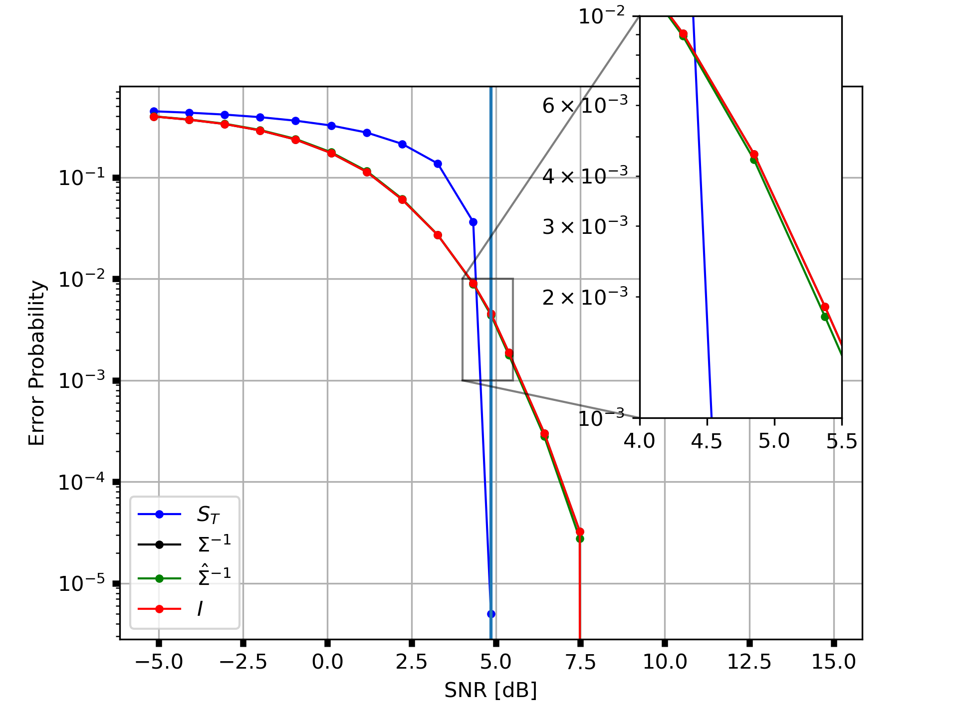
   Figure 3: Additive noise channel with a two-dimensional noise comprised of a Gaussian component and a uniform component. Error probability vs. various SNRs [dB].

2. Two-dimensional Gaussian mixture noise: We perform a simulation similar to the previous example, where now the codebook is a $64$-QAM constellation in $2$D [52, Fig. 2, (c)], and $Z\in\mathbb{R}^{2}$ is a zero-mean Gaussian Mixture noise of $l=2$ components $Z_{i}\sim\mathcal{N}(0,K_{i})$, and mixture weights $\{\omega_{i}\}_{i=1}^{l}$. The right panel of Fig. 4 displays the error probability of the final hypothesis decoder, under various SNR values. In Fig. 4, we observe that the error probability scales similarly for both $S_{T}$ and $\Sigma^{-1}=\left(\frac{1}{l}\sum_{i=1}^{l}\omega_{i}K_{i}\right)^{-1}$, even for SNR values that are significantly smaller than the training SNR. This shows the generalization of the learned decoder, which is a desired trait for systems where the SNR at operation time is unknown durning training.

   $d$	$m$	$n_{\text{train}}$	$n_{\text{batch}}$	$T$	$n_{\text{test}}$	$\lambda$	$\text{SNR}_{\text{train}}$
   $2$	$64$	$220$	$5$	$10^{3}$	$10^{4}$	$10^{-7}$	$22.34$

   Table II: Additive noise channel with a two-dimensional Gaussian mixture noise. Experiment parameters.

   

   

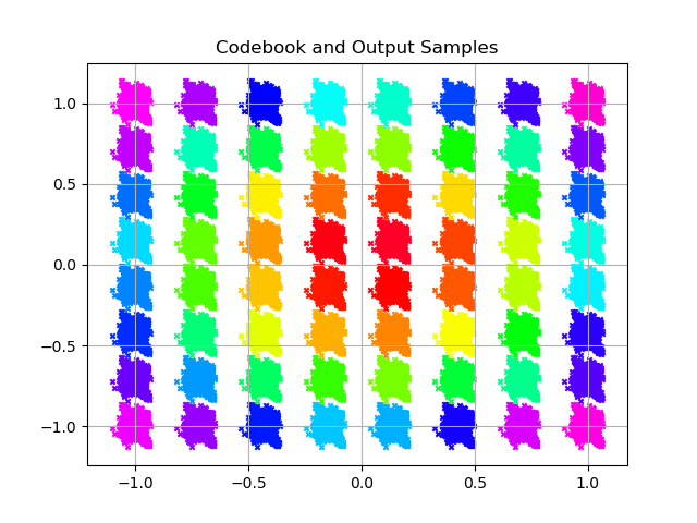
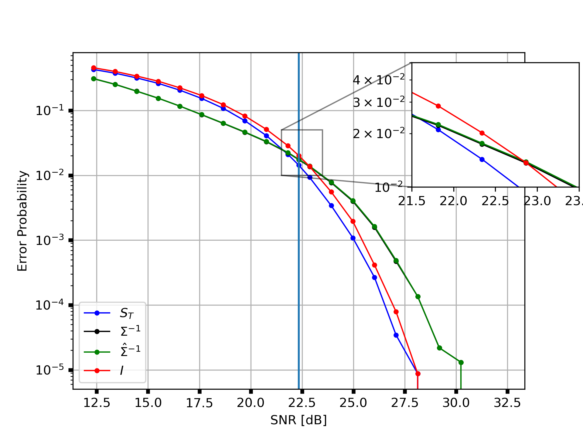
   Figure 4: Additive noise channel with a two-dimensional Gaussian mixture noise. Left: the test samples in SNR 27 [dB]. Right: error probability vs. various SNRs [dB].

VI-B Stochastic Sub-gradient Descent Algorithm for the Non-Linear White Gaussian Noise Channel

The algorithm’s performance, for the non-linear channel, is compared with a NN decoder using the real transformation $f(\cdot)$, which is the maximum likelihood decoder, and a NN decoder using the mean of the transformed samples of each codeword as the transformed value of the codeword, denoted $\mu_{X}$. We denote by $H_{T}$ the hypothesis chosen during the training phase, whether it is the hypothesis generated at iteration $T$ or at another iteration, guided by cross validation over the training samples.

1. Two-dimensional linear channel: Assume $d=2$, a codebook of $m=8$ codewords as proposed in [52, Fig. 2, (a)], and a linear and invertible channel transformation

   $$f\begin{pmatrix}x_{1}\\ x_{2}\end{pmatrix}=\left(\begin{array}[]{cc}1.04&0.19\\ 0.19&1.96\end{array}\right)\begin{pmatrix}x_{1}\\ x_{2}\end{pmatrix}.$$ (33)

   In this simple example, the optimal matrix is obviously $H=\left(\begin{array}[]{cc}1.04&0.19\\ 0.19&1.96\end{array}\right)$. The training samples are shown in the left panel of Fig. 5, and the right panel displays the error probability of the final hypothesis decoder, under various SNR values. The right panel shows that the learned decoder’s performance is practically the same as that of the optimal decoder. The experiment parameters are listed in Table III.

   $d$	$m$	$n_{\text{train}}$	$n_{\text{batch}}$	$T$	$n_{\text{test}}$	$\lambda$	$\text{SNR}_{\text{train}}$
   $2$	$8$	$1.6\cdot 10^{3}$	$10$	$1.4\cdot 10^{3}$	$10^{4}$	$(10^{-3},10^{-4})$	$3.74$

   Table III: Two-dimensional linear white Gaussian noise channel. Experiment parameters.

   

   

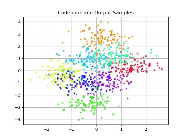
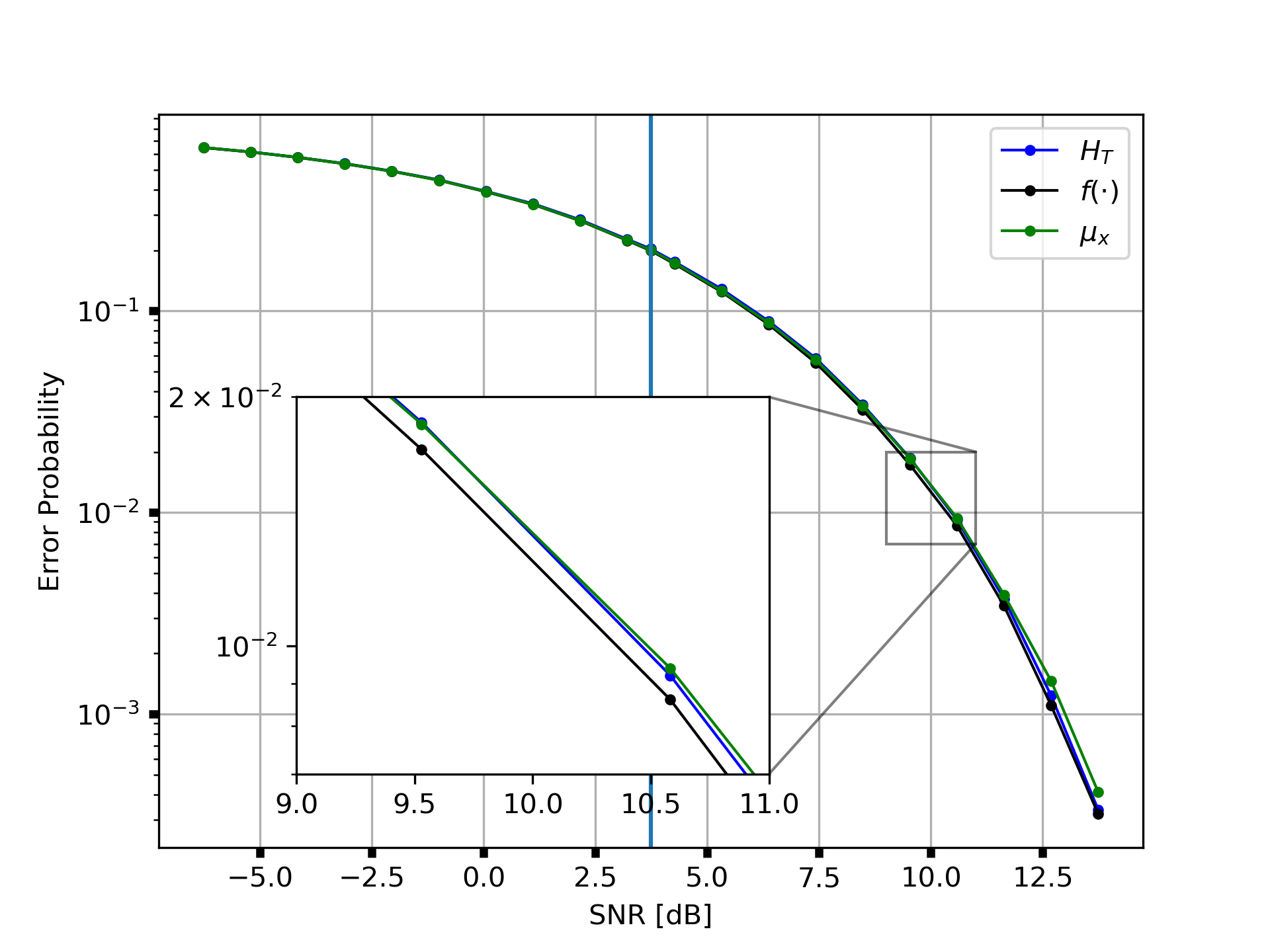
   Figure 5: Two-dimensional linear white Gaussian noise channel. Left: codewords (circles) and output samples (X’s). Right: error probability vs. various SNRs [dB].

2. Two-dimensional non-linear channel: We perform a simulation similar to the previous example, where now the channel transformation is non-linear

   $$f\begin{pmatrix}x_{1}\\ x_{2}\end{pmatrix}=\left(\begin{array}[]{ccc}0.94&0.07&0.15\\ 0.46&0.72&0.4\end{array}\right)\begin{pmatrix}x_{1}\\ x_{2}\\ x_{1}x_{2}\end{pmatrix}.$$ (34)

   In this example, the learner is required to learn a linear transformation which approximates the non-linear channel transformation. The training samples are shown in the left panel of Fig. 6, and the right panel displays the error probability of the final hypothesis decoder, under various SNR values. The right panel shows that the learned decoder’s performance is close to that of the optimal decoder, however the performance gap increases with the SNR. This shows the difficulty of learning a decoder for a non-linear channel, compared to the linear channel from the previous experiment. The experiment parameters are listed in Table IV.

   $d$	$m$	$n_{\text{train}}$	$n_{\text{batch}}$	$T$	$n_{\text{test}}$	$\lambda$	$\text{SNR}_{\text{train}}$
   $2$	$8$	$1.6\cdot 10^{3}$	$10$	$3\cdot 10^{3}$	$10^{4}$	$(10^{-2},10^{-3})$	$11.7$

   Table IV: Two-dimensional non-linear white Gaussian noise channel. Experiment parameters.

   

   

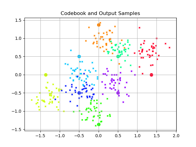
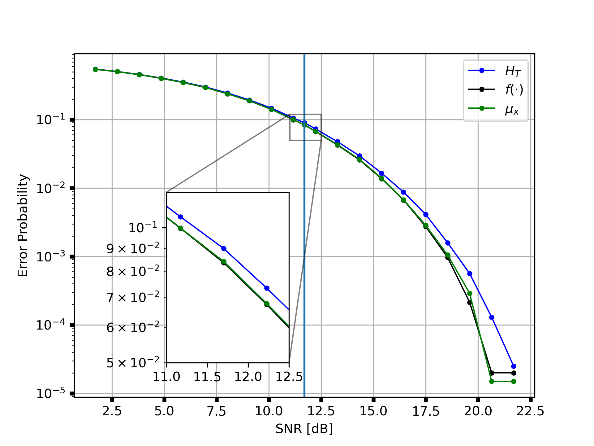
   Figure 6: Two-dimensional non-linear white Gaussian noise channel. Left: codewords (circles) and output samples (X’s). Right: error probability vs. various SNRs [dB].

VII Summary and Future Research

In this section, we summarize the main results of the paper, point out some open problems and propose ideas for future research.

In Sec. III we have derived an RLM problem for learning a maximum margin NN decoder. We have developed a convex lower bound to the maximum margin problem which can be efficiently solved. Specifically, in step 2 we used a lower bound in order to simplify the difficult, non-convex in general, problem. A goal for future research is to consider methods to tighten this lower bound. For example, such a method can be based on elimination of irrelevant codeword-pairs, e.g., far apart pairs connected with a line in the same direction as the line connecting a closer pair. In the derivation for the non-linear Gaussian noise channel, a linearization of the decoder was proposed as a part of the derivation of the minimum norm problem. Future research could study other derivations of minimum norm formulations, which are suitable for non-linear classifiers.

Next, in Sec. IV, we have proved an expected generalization error bound for the error probability loss. The stated generalization error bound holds only on average, and a goal for future research is to prove a generalization bound which holds with high probability. Such generalization bounds were recently proved for SVM in [53], possibly the same methods could be used for this problem. Another possibility for improving the generalization bound is by making assumptions on the noise distribution, similar to what was established for vector quantizers in [40, 37, 38, 39].

For channels with complicated non-linear transformations, a linear kernel might perform poorly. Nonetheless, it is possible to enrich the expressive power of the NN decoder, by first mapping the codewords into a high-dimensional feature space [21, Ch. 16]. If such a mapping is applied to the codebook, then the matrices dimensions will increase accordingly, $\mathcal{H}=\mathbb{R}^{d_{y}\times D_{x}}$ and $\mathcal{K}=\mathbb{S}^{D_{x}\times D_{x}}$. Therefore, a hypothesis will be determined by $O\left(d_{y}D_{x}+D_{x}^{2}\right)$ parameters. Furthermore, the complexity of every operation involving codewords would increase significantly. These computations become infeasible when the mapping is to an infinite dimension feature space. As well known, in order to alleviate this dimensionality problem, one can use the kernel trick [21, Ch. 16.2] for the non-linear channel model. In this regard, it can be shown that the RLM and its solution, the decoder, can be expressed solely by the kernel function and the samples. However, the constraint $H^{T}H\preccurlyeq K$ cannot be easily expressed in terms of the kernel. It is a goal for future research to solve this problem and enable the use of a kernel trick in this problem.

In Sec. V, we proposed a stochastic sub-gradient descent algorithm for solving the RLM problem. This algorithm involves a projection step in each iteration. While the complexity of the projection is independent of the sample size, it still poses a hard computational requirement for high-dimensional problems. The projection step in the non-linear channel model stems from the linearization of the decoder, and therefore it might be unnecessary for alternative variants of minimum norm problems.

Finally, a different direction for future research is exploring the margin properties of DNNs in the context of the decoder learning problem. For classification problems, it was recently identified that the large margin principle is beneficial to the generalization ability of DNNs (see, e.g., the survey [54] and references therein). It is of interest to identify similar properties for the decoder learning problem.

Appendix A Derivations for Section III

In this appendix, we provide the proofs for the derivation of the RLM for the additive noise channel (Appendix A-A), and provide the development steps and proofs for the non-linear channel (Appendix A-B).

A-A Proofs for the Additive Noise Channel RLM problem

We start by justifying the margin based objective (step 1) by proving claim 2.

Proof:

Consider the decision regions of a given codeword-pair $x_{p},x_{q}\in C$

$$\left\|x_{p}-y\right\|_{S}\stackrel{{\scriptstyle[}}{{p}}]{q}{\gtrless}\left\|x_{q}-y\right\|_{S}\iff\left(y-\frac{1}{2}\left(x_{p}+x_{q}\right)\right)^{T}S\delta_{pq}\stackrel{{\scriptstyle[}}{{q}}]{p}{\gtrless}0.$$ (35)

Note that the factor $-\frac{1}{2}(x_{p}+x_{q})$ centers the codebook and accordingly the subset $\boldsymbol{D}_{p}\bigcup\boldsymbol{D}_{q}$ of that dataset. We remain with a linear classifier $\bar{y}S\delta_{pq}\stackrel{{\scriptstyle[}}{{q}}]{p}{\gtrless}0$ for the centered samples $\bar{y}\triangleq y-\frac{1}{2}(x_{p}+x_{q})$. By using [21, Claim 15.1] we get that the distance between a point $v$ and the hyperplane with normal vector $S\delta_{pq}$ is

$$\frac{\left|v^{T}S\delta_{pq}\right|}{\left\|S\delta_{pq}\right\|}.$$ (36)

Therefore, the margin induced by $S$ for the codeword-pair $p,q$ is

$$\min_{i\in\boldsymbol{D}_{p}\cup\boldsymbol{D}_{q}}\frac{\left|\left(y_{i}-\frac{1}{2}\left(x_{p}+x_{q}\right)\right)^{T}S\delta_{pq}\right|}{\left\|S\delta_{pq}\right\|}.$$ (37)

Taking the minimum over all codeword-pairs and maximizing over $S$ gives

$$\max_{S\in\mathbb{S}_{+}}\min_{1\leq p<q\leq m}\min_{i\in\boldsymbol{D}_{p}\cup\boldsymbol{D}_{q}}\frac{\left|\left(y_{i}-\frac{1}{2}\left(x_{p}+x_{q}\right)\right)^{T}S\delta_{pq}\right|}{\left\|S\delta_{pq}\right\|}.$$ (38)

Under the assumption of separability we can equivalently write

$$\max_{S\in\mathbb{S}_{+}}\min_{1\leq p<q\leq m}\min_{i\in\boldsymbol{D}_{p}\cup\boldsymbol{D}_{q}}\left(-1\right)^{\mathbb{I}\left(i\in\boldsymbol{D}_{q}\right)}\frac{\left(y_{i}-\frac{1}{2}\left(x_{p}+x_{q}\right)\right)^{T}S\delta_{pq}}{\left\|S\delta_{pq}\right\|}.$$ (39)

∎

We proceed to show the lower bound validity (step 2) by proving claim 3.

Proof:

Due to invariance to scaling of $S$ in (12), we can add the constraint $\max_{1\leq p<q\leq m}\left\|S\delta_{pq}\right\|\leq 1$ (from (13)), and get an equivalent problem. Under this constraint

$$\max_{S\in\mathbb{S}_{+}}\min_{1\leq p<q\leq m}\min_{i\in\boldsymbol{D}_{p}\cup\boldsymbol{D}_{q}}\left(-1\right)^{\mathbb{I}\left(i\in\boldsymbol{D}_{q}\right)}\left(y_{i}-\frac{1}{2}\left(x_{p}+x_{q}\right)\right)^{T}S\delta_{pq}\\ \leq\max_{S\in\mathbb{S}_{+}}\min_{1\leq p<q\leq m}\min_{i\in\boldsymbol{D}_{p}\cup\boldsymbol{D}_{q}}\left(-1\right)^{\mathbb{I}\left(i\in\boldsymbol{D}_{q}\right)}\frac{\left(y_{i}-\frac{1}{2}\left(x_{p}+x_{q}\right)\right)^{T}S\delta_{pq}}{\left\|S\delta_{pq}\right\|},$$ (40)

which directly leads to the claim. ∎

Now we turn to prove the equivalent minimum norm formulation (step 3). This is done by proving Lemma 4.

Proof:

Let $S^{*}$ be a solution of (13) and $\gamma^{*}$ be its margin value, i.e.,

$$\gamma^{*}=\min_{1\leq p<q\leq m}\min_{i\in\boldsymbol{D}_{p}\cup\boldsymbol{D}_{q}}a_{pqi}^{T}S^{*}\delta_{pq}.$$ (41)

Let $S^{\#}$ be the solution to (14) and denote

$$\hat{S}\triangleq\frac{S^{\#}}{\max_{1\leq p<q<m}\left\|S^{\#}\delta_{pq}\right\|}.$$ (42)

We will show that $\hat{S}$ is a solution to (13).

First, we show that $\hat{S}$ achieves a margin value of at least $\gamma^{*}$. By definition of $\gamma^{*}$ we have that for all $1\leq p<q\leq m,i\in\boldsymbol{D}_{p}\cup\boldsymbol{D}_{q}$ it holds that $a_{pqi}^{T}\frac{S^{*}}{\gamma^{*}}\delta_{pq}\geq 1$. Hence, $\frac{S^{*}}{\gamma^{*}}$ satisfies the constraint in (14), combined with $S^{\#}$ being a minimizer for (14) it yields

$$\max_{1\leq p<q\leq m}\left\|S^{\#}\delta_{pq}\right\|^{2}\leq\max_{1\leq p<q\leq m}\left\|\frac{S^{*}}{\gamma^{*}}\delta_{pq}\right\|^{2}.$$ (43)

Using this, we can bound

$$\max_{1\leq p<q\leq m}\left\|S^{\#}\delta_{pq}\right\|\overset{\eqref{eq:norm compare}}{\leq}\max_{1\leq p<q\leq m}\left\|\frac{S^{*}}{\gamma^{*}}\delta_{pq}\right\|=\frac{1}{\gamma^{*}}\max_{1\leq p<q\leq m}\left\|S^{*}\delta_{pq}\right\|\leq\frac{1}{\gamma^{*}},$$ (44)

where the last inequality is due to $S^{*}$ satisfying the constraint $\left\|S^{*}\delta_{pq}\right\|\leq 1$ for all $1\leq p<q\leq m,i\in\boldsymbol{D}_{p}\cup\boldsymbol{D}_{q}$. It follows that for all $1\leq p<q\leq m,i\in\boldsymbol{D}_{p}\cup\boldsymbol{D}_{q}$

$$a_{pqi}^{T}\hat{S}\delta_{pq}=\frac{1}{\max_{1\leq p<q\leq m}\left\|S^{\#}\delta_{pq}\right\|}a_{pqi}^{T}S^{\#}\delta_{pq}\overset{(a)}{\geq}\frac{1}{\max_{1\leq p<q\leq m}\left\|S^{\#}\delta_{pq}\right\|}\overset{(b)}{\geq}\gamma^{*},$$ (45)

where $(a)$ is due to $S^{\#}$ satisfying the constraint $a_{pqi}^{T}S\delta_{pq}\geq 1$ for all $1\leq p<q\leq m,i\in\boldsymbol{D}_{p}\cup\boldsymbol{D}_{q}$, and $(b)$ follows from (44).

Second, $\hat{S}$ complies with the constraints of (13), since, by definition

$$\max_{1\leq p<q\leq m}\left\|\hat{S}\delta_{pq}\right\|=\max_{1\leq p<q<m}\left\|\frac{S^{\#}}{\max_{0\leq p<q\leq m}\left\|S^{\#}\delta_{pq}\right\|}\delta_{pq}\right\|=1.$$ (46)

Notice that due to invariance to scaling, in a NN decoder, using $S^{\#}$ is equivalent to using $\hat{S}$. Maximizing $\left\|S\delta_{pq}\right\|$ is equivalent to maximizing $\left\|S\delta_{pq}\right\|^{2}$. This argument completes the proof. ∎

We next consider step 4, and show that relaxing the separability assumption of a minimum norm problem leads to an RLM problem. To this end, we allow the constraints in the minimum norm problem (14) to be violated by adding non-negative slack variables $\{\xi_{pqi}\}$, one for each sample. We penalize for violations by minimizing over the slack variables and add $\lambda$ as a regularization parameter that controls the tradeoff between the two terms. This leads to the following optimization problem

$$\begin{array}[]{ccc}\min_{S\in\mathbb{S}_{+}}\min_{\{\xi_{pqi}\}}&\lambda\max_{0\leq p<q<m}\left\|S\delta_{pq}\right\|^{2}+\sum_{\begin{subarray}{c}1\leq p<q\leq m\\ i\in\boldsymbol{D}_{p}\cup\boldsymbol{D}_{q}\end{subarray}}\xi_{pqi}\\ \operatorname{subject\;to}&a_{pqi}^{T}S\delta_{pq}\geq 1-\xi_{pqi}&\forall\,1\leq p<q\leq m,\,i\in\boldsymbol{D}_{p}\cup\boldsymbol{D}_{q}.\\ &\xi_{pqi}\geq 0&\forall\,1\leq p<q\leq m,\,i\in\boldsymbol{D}_{p}\cup\boldsymbol{D}_{q}\end{array}$$ (47)

For any $1\leq p<q\leq m,i\in\boldsymbol{D}_{p}\cup\boldsymbol{D}_{q}$ either $a_{pqi}^{T}S\delta_{pq}\geq 1$ and then $\xi_{pqi}=0$, or $a_{pqi}^{T}S\delta_{pq}<1$ and then $\xi_{pqi}=1-a_{pqi}^{T}S\delta_{pq}$. Substituting $\xi_{pqi}=\max\{0,1-a_{pqi}^{T}S\delta_{pq}\}$ in (47) gives (15).

A-B Development Steps and Proofs for The Non-linear White Gaussian Channel

We next develop an RLM problem from a maximum margin approach for the non-linear white Gaussian noise channel. The derivation follows the same general steps as the ones for the additive noise channel in Sec. III-A, and so we omit details whenever they are similar to that of Sec. III-A. Nonetheless, we highlight the step of developing a minimum norm formulation (Step 3), since it is delicate due to the quadratic form of the decoder, and so requires an additional approximation step.

Step 1 – maximization of the minimum margin

As before, we begin with the assumption that the dataset $\boldsymbol{D}$ is separable, which means here that there exists a decoder $H$ that achieves zero loss over $\boldsymbol{D}$, and this assumption will be relaxed in the following steps. Now, the learner’s goal is to find a decoder $H$ that maximizes the minimum margin, over all transformed codeword-pairs $Hx_{p},Hx_{q}\in C$. This margin-maximization problem is given as follows:

Claim 10.

The maximum margin induced by a decoder $H$ is

$$\max_{H\in\mathcal{H}}\min_{i\in[n]}\min_{j^{\prime}\in[m]\backslash\{j_{i}\}}\frac{y_{i}^{T}H\delta_{j_{i}j^{\prime}}-\frac{1}{2}\left(x_{j_{i}}+x_{j^{\prime}}\right)^{T}H^{T}H\delta_{j_{i}j^{\prime}}}{\left\|H\delta_{j_{i}j^{\prime}}\right\|}.$$ (48)

Proof:

For every codeword-pair $x_{p},x_{q}\in C$ the decision regions are

$$\left\|y-Hx_{p}\right\|\stackrel{{\scriptstyle[}}{{p}}]{q}{\gtrless}\left\|y-Hx_{q}\right\|\iff y^{T}H\delta_{pq}-\frac{1}{2}\left(x_{p}+x_{q}\right)^{T}H^{T}H\delta_{pq}\stackrel{{\scriptstyle[}}{{q}}]{p}{\gtrless}0.$$ (49)

Using analogous arguments to those used in the proof of Claim 2 completes the proof. ∎

Step 2 – a lower bound

The problem (48) is not necessarily convex and is hard to solve directly. Therefore, we proceed to maximize the following lower bound on its value. Unlike the analogous lower bound in Sec. III-A, finding this lower bound is not a convex optimization problem, but it still serves as a useful step for next derivations. We denote $r_{x}=\max_{j\in[m]}\|x_{j}\|$ and $R_{x}=\max_{j\in[m]}\|f(x_{j})\|$.

Claim 11.

The value of the problem

$$\begin{array}[]{cc}\max_{H\in\mathcal{H}}\min_{i\in\left[n\right]}\min_{j^{\prime}\in\left[m\right]\backslash\left\{j_{i}\right\}}&y_{i}^{T}H\delta_{j_{i}j^{\prime}}-\frac{1}{2}\left(x_{j_{i}}+x_{j^{\prime}}\right)^{T}H^{T}H\delta_{j_{i}j^{\prime}}\\ \operatorname{subject\;to}&\max_{1\leq p<q\leq m}\left\|H\delta_{pq}\right\|\leq\sqrt{\frac{r_{x}^{2}}{r_{x}^{2}+R_{x}^{2}}}\end{array}$$ (50)

is a lower bound on the value of (48).

The proof is similar to the proof for claim 3. We note, however, that since the current considered class of decoders is not scale-invariant, we suspect that this lower bound might be less tight in general. So tightening of this bound is an interesting open problem.

Proof:

By adding the constraint

$$\max_{1\leq p<q\leq m}\left\|H\delta_{pq}\right\|\leq\sqrt{\frac{r_{x}^{2}}{r_{x}^{2}+R_{x}^{2}}},$$ (51)

we effectively restrict the hypothesis class without increasing the value of the problem. This is since $\sqrt{\frac{r_{x}^{2}}{r_{x}^{2}+R_{x}^{2}}}<1$ and so under this additional constraint

$$\max_{\left(H,K\right)\in\mathcal{H}\times\mathcal{K}}\min_{i\in\left[n\right]}\min_{j^{\prime}\in\left[m\right]\backslash\left\{j_{i}\right\}}y_{i}^{T}H\delta_{j_{i}j^{\prime}}-\frac{1}{2}\left(x_{j_{i}}+x_{j^{\prime}}\right)^{T}H^{T}H\delta_{j_{i}j^{\prime}}\\ \leq\max_{\left(H,K\right)\in\mathcal{H}\times\mathcal{K}}\min_{i\in\left[n\right]}\min_{j^{\prime}\in\left[m\right]\backslash\left\{j_{i}\right\}}\frac{y_{i}^{T}H\delta_{j_{i}j^{\prime}}-\frac{1}{2}\left(x_{j_{i}}+x_{j^{\prime}}\right)^{T}H^{T}H\delta_{j_{i}j^{\prime}}}{\left\|H\delta_{j_{i}j^{\prime}}\right\|}.$$ (52)

This directly leads to the claim. ∎

Step 3 – minimum norm formulation

As we have seen, obtaining an RLM problem and the removal of the separability assumption is done via a minimum norm formulation. In order to obtain a minimum norm formulation, the objective function should be linear in the parameter determining the decoder, yet (50) violates this requirement. We therefore resort to the the following approximation strategy. First, we write $K=H^{T}H\in\mathcal{K}\triangleq\mathbb{S}_{+}^{d_{x}}$ and thus linearize the decoder’s parametrization. We then drop this constraint, yet add a judicious constraint on $\max_{1\leq p<q\leq m}\left\|H\delta_{pq}\right\|^{2}+\max_{1\leq p^{\prime}<q^{\prime}\leq m}\left\|K\delta_{p^{\prime}q^{\prime}}\right\|^{2}$, which replaces the constraint $\max_{1\leq p<q\leq m}\|H\delta_{pq}\|\leq\sqrt{\frac{r_{x}^{2}}{r_{x}^{2}+R_{x}^{2}}}$ in (50). With this approximation, we then convert the problem (50) to a minimum norm problem. Then, since the learned decoder will eventually use a learned linear kernel $H$ and will (implicitly) set $K=H^{T}H$, we re-introduce the constraint $K=H^{T}H$, but in a convex-relaxed form $H^{T}H\preceq K$.

Specifically, we choose the constraint on $\max_{1\leq p<q\leq m}\left\|H\delta_{pq}\right\|^{2}+\max_{1\leq p^{\prime}<q^{\prime}\leq m}\left\|K\delta_{p^{\prime}q^{\prime}}\right\|^{2}$ as follows: Since the channel transformation $f$ increases the norm of $x$ by a factor of at most $R_{x}/r_{x}$ it is reasonable to bound $\lambda_{\max}(H)\leq\frac{R_{x}}{r_{x}}$. Now, the constraint on $H$ in (50) implies that

$$\max_{1\leq p<q\leq m}\delta_{pq}^{T}K\delta_{pq}=\max_{1\leq p<q\leq m}\left\|H\delta_{pq}\right\|^{2}\leq\frac{r_{x}^{2}}{r_{x}^{2}+R_{x}^{2}}.$$ (53)

Then,

$$\max_{1\leq p<q\leq m}\left\|K\delta_{pq}\right\|^{2}\leq\lambda_{\max}(K)\cdot\max_{1\leq p<q\leq m}\delta_{pq}^{T}K\delta_{pq}\leq\frac{R_{x}^{2}}{r_{x}^{2}+R_{x}^{2}},$$ (54)

which holds since $K\in{\cal K}$ is symmetric. By replacing the constraint in (50), we get the following problem

$$\begin{array}[]{cc}\max_{(H,K)\in\mathcal{H}\times\mathcal{K}}\min_{i\in\left[n\right]}\min_{j^{\prime}\in\left[m\right]\backslash\left\{j_{i}\right\}}&y_{i}^{T}H\delta_{j_{i}j^{\prime}}-\frac{1}{2}\left(x_{j_{i}}+x_{j^{\prime}}\right)^{T}K\delta_{j_{i}j^{\prime}}\\ \operatorname{subject\;to}&\max_{1\leq p<q\leq m}\left\|H\delta_{pq}\right\|^{2}+\max_{1\leq p^{\prime}<q^{\prime}\leq m}\left\|K\delta_{p^{\prime}q^{\prime}}\right\|^{2}\leq 1.\end{array}$$ (55)

The formulation (55) then leads to a minimum norm problem, as desired.

Lemma 12.

Every solution to the following minimum norm problem

$$\begin{array}[]{cc}\min_{(H,K)\in\mathcal{H}\times\mathcal{K}}&\max_{\begin{subarray}{c}1\leq p<q\leq m\\ 1\leq p^{\prime}<q^{\prime}\leq m\end{subarray}}\left\|H\delta_{pq}\right\|^{2}+\left\|K\delta_{p^{\prime}q^{\prime}}\right\|^{2}\\ \operatorname{subject\;to}&\min_{i\in[n]}\min_{j^{\prime}\in[m]\backslash\{j_{i}\}}y_{i}^{T}H\delta_{j_{i}j^{\prime}}-\frac{1}{2}\left(x_{j_{i}}+x_{j^{\prime}}\right)^{T}K\delta_{j_{i}j^{\prime}}\geq 1,\end{array}$$ (56)

is a solution to (55).

The proof of Lemma 12 shares similar structure to the proof of Lemma 4 but it is more delicate, due to the more complicated parametrization of the linearized decoder.

Proof:

Let $(H^{*},K^{*})$ be a solution of (55) and $\gamma^{*}$ its margin value, i.e.,

$$\gamma^{*}=\min_{i\in[n]}\min_{j^{\prime}\in[m]\backslash\{j_{i}\}}y_{i}^{T}H\delta_{j_{i}j^{\prime}}-\frac{1}{2}\left(x_{j_{i}}+x_{j^{\prime}}\right)^{T}K\delta_{j_{i}j^{\prime}}.$$ (57)

Let $(H^{\#},K^{\#})$ be a solution to (56) and denote the corresponding normalized solution

$$\hat{H}\triangleq\frac{H^{\#}}{\sqrt{\max_{1\leq p<q\leq m}\left\|H^{\#}\delta_{pq}\right\|^{2}+\max_{1\leq p^{\prime}<q^{\prime}\leq m}\left\|K^{\#}\delta_{p^{\prime}q^{\prime}}\right\|^{2}}},$$ (58)

and

$$\hat{K}\triangleq\frac{K^{\#}}{\sqrt{\max_{1\leq p<q\leq m}\left\|H^{\#}\delta_{pq}\right\|^{2}+\max_{1\leq p^{\prime}<q^{\prime}\leq m}\left\|K^{\#}\delta_{p^{\prime}q^{\prime}}\right\|^{2}}}.$$ (59)

We will show that $(\hat{H},\hat{K})$ is a solution to (55).

First, we show that $(\hat{H},\hat{K})$ achieves a margin value of at least $\gamma^{*}$. By definition of $\gamma^{*}$ we have that for all $i\in[n],j^{\prime}\in[m]\backslash\{j_{i}\}$:

$$y_{i}^{T}\frac{H^{*}}{\gamma^{*}}\delta_{j_{i}j^{\prime}}-\frac{1}{2}\left(x_{j_{i}}+x_{j^{\prime}}\right)^{T}\frac{K^{*}}{\gamma^{*}}\delta_{j_{i}j^{\prime}}\geq 1.$$ (60)

Hence, $(\frac{H^{*}}{\gamma^{*}},\frac{K^{*}}{\gamma^{*}})$ satisfies the constraint in (56). Combined with $(H^{\#},K^{\#})$ being a minimizer for (56), it yields

$$\max_{1\leq p<q\leq m}\left\|H^{\#}\delta_{pq}\right\|^{2}+\max_{1\leq p^{\prime}<q^{\prime}\leq m}\left\|K^{\#}\delta_{p^{\prime}q^{\prime}}\right\|^{2}\leq\max_{1\leq p<q\leq m}\left\|\frac{H^{*}}{\gamma^{*}}\delta_{pq}\right\|^{2}+\max_{1\leq p^{\prime}<q^{\prime}\leq m}\left\|\frac{K^{*}}{\gamma^{*}}\delta_{p^{\prime}q^{\prime}}\right\|^{2}.$$ (61)

Using this we can bound

$$\max_{1\leq p<q\leq m}\left\|H^{\#}\delta_{pq}\right\|^{2}+\max_{1\leq p^{\prime}<q^{\prime}\leq m}\left\|K^{\#}\delta_{p^{\prime}q^{\prime}}\right\|^{2} \overset{\eqref{eq:norm compare-1}}{\leq}\max_{1\leq p<q\leq m}\left\|\frac{H^{*}}{\gamma^{*}}\delta_{pq}\right\|^{2}+\max_{1\leq p^{\prime}<q^{\prime}\leq m}\left\|\frac{K^{*}}{\gamma^{*}}\delta_{p^{\prime}q^{\prime}}\right\|^{2}$$ (62)

$$=\left(\frac{1}{\gamma^{*}}\right)^{2}\max_{1\leq p<q\leq m}\left\|H^{*}\delta_{pq}\right\|^{2}+\left(\frac{1}{\gamma^{*}}\right)^{2}\max_{1\leq p^{\prime}<q^{\prime}\leq m}\left\|K^{*}\delta_{p^{\prime}q^{\prime}}\right\|^{2}$$ (63)

$$\leq\left(\frac{1}{\gamma^{*}}\right)^{2},$$ (64)

where the last inequality is due to $(H^{*},K^{*})$ satisfying the constraints of (55). It follows that for all $i\in[n],j^{\prime}\in[m]\backslash\{j_{i}\}$:

$$y_{i}^{T}\hat{H}\delta_{j_{i}j^{\prime}}-\frac{1}{2}\left(x_{j_{i}}+x_{j^{\prime}}\right)^{T}\hat{K}\delta_{j_{i}j^{\prime}} =\frac{y_{i}^{T}H^{\#}\delta_{j_{i}j^{\prime}}-\frac{1}{2}\left(x_{j_{i}}+x_{j^{\prime}}\right)^{T}K^{\#}\delta_{j_{i}j^{\prime}}}{\sqrt{\max_{1\leq p<q\leq m}\left\|H^{\#}\delta_{pq}\right\|^{2}+\max_{1\leq p^{\prime}<q^{\prime}\leq m}\left\|K^{\#}\delta_{p^{\prime}q^{\prime}}\right\|^{2}}}$$ (65)

$$\overset{(a)}{\geq}\frac{1}{\sqrt{\max_{1\leq p<q\leq m}\left\|H^{\#}\delta_{pq}\right\|^{2}+\max_{1\leq p^{\prime}<q^{\prime}\leq m}\left\|K^{\#}\delta_{p^{\prime}q^{\prime}}\right\|^{2}}}$$ (66)

$$\overset{(b)}{\geq}\gamma^{*},$$ (67)

where $(a)$ is due to $(H^{\#},K^{\#})$ satisfying the constraint

$$y_{i}^{T}H^{\#}\delta_{j_{i}j^{\prime}}-\frac{1}{2}\left(x_{j_{i}}+x_{j^{\prime}}\right)^{T}K^{\#}\delta_{j_{i}j^{\prime}}\geq 1$$ (68)

for all $i\in[n],j^{\prime}\in[m]\backslash\{j_{i}\}$, and $(b)$ follows from (62).

Second, we show that $(\hat{H},\hat{K})$ complies with the constraints of (55). By definition

$$\max_{1\leq p<q\leq m}\left\|\hat{H}\delta_{pq}\right\|^{2}+\max_{1\leq p^{\prime}<q^{\prime}\leq m}\left\|\hat{K}\delta_{p^{\prime}q^{\prime}}\right\|^{2}=\frac{\max_{1\leq p<q\leq m}\left\|H^{\#}\delta_{pq}\right\|^{2}+\max_{1\leq p^{\prime}<q^{\prime}\leq m}\left\|K^{\#}\delta_{p^{\prime}q^{\prime}}\right\|^{2}}{\max_{1\leq p<q\leq m}\left\|H^{\#}\delta_{pq}\right\|^{2}+\max_{1\leq p^{\prime}<q^{\prime}\leq m}\left\|K^{\#}\delta_{p^{\prime}q^{\prime}}\right\|^{2}}=1.$$ (69)

As evident from (48) with $H^{T}H$ replaced by $K$, the problem is scale invariant and so using $(H^{\#},K^{\#})$ is equivalent to using $(\hat{H},\hat{K})$. ∎

As said, after obtaining a minimum norm formulation (56) we add the convex constraint $H^{T}H\preceq K$.

Step 4 – relaxation of the separability assumption

Next, we introduce slack variables in order to relax the assumption that the dataset $\boldsymbol{D}$ is separable. To this end, we allow the constraints in the minimum norm problem to be violated by adding non-negative slack variables $\{\xi_{ij^{\prime}}\}$, one for each sample. We penalize for violations by minimizing over the slack variables and add $\lambda$ as a regularization parameter. This leads to the following optimization problem

$$\begin{array}[]{cc}\min_{\left(H,K\right)\in\mathcal{H}\times\mathcal{K}}\min_{\left\{\xi\right\}}&\lambda\left[\max_{1\leq p<q\leq m}\left\|H\delta_{pq}\right\|^{2}+\max_{1\leq p^{\prime}<q^{\prime}\leq m}\left\|K\delta_{p^{\prime}q^{\prime}}\right\|^{2}\right]+\sum_{i\in\left[n\right]}\sum_{j^{\prime}\in\left[m\right]\backslash\left\{j_{i}\right\}}\xi_{ij^{\prime}}\\ \operatorname{subject\;to}&y_{i}^{T}H\delta_{j_{i}j^{\prime}}-\frac{1}{2}\left(x_{j_{i}}+x_{j^{\prime}}\right)^{T}K\delta_{j_{i}j^{\prime}}\geq 1-\xi_{ij^{\prime}}\\ &\xi_{ij^{\prime}}\geq 0\end{array}.$$ (70)

For any $i\in[n],j^{\prime}\in[m]\backslash\{j_{i}\}$ either $y_{i}^{T}H\delta_{j_{i}j^{\prime}}-\frac{1}{2}(x_{j_{i}}+x_{j^{\prime}})^{T}K\delta_{j_{i}j^{\prime}}\geq 1$ and then $\xi_{ij^{\prime}}=0$, or $y_{i}^{T}H\delta_{j_{i}j^{\prime}}-\frac{1}{2}(x_{j_{i}}+x_{j^{\prime}})^{T}K\delta_{j_{i}j^{\prime}}<1$ and then $\xi_{ij^{\prime}}=1-[y_{i}^{T}H\delta_{j_{i}j^{\prime}}-\frac{1}{2}(x_{j_{i}}+x_{j^{\prime}})^{T}K\delta_{j_{i}j^{\prime}}]$. By substituting

$$\xi_{ij^{\prime}}=\max\left\{0,1-\left[y_{i}^{T}H\delta_{j_{i}j^{\prime}}-\frac{1}{2}\left(x_{j_{i}}+x_{j^{\prime}}\right)^{T}K\delta_{j_{i}j^{\prime}}\right]\right\}$$ (71)

in (70), the problem (70) is equivalent to the RLM problem for the hinge loss function $\mathring{\ell}^{\text{hinge}}(H,K,i)$ in (17). The RLM problem is then given by

$$\begin{array}[]{cc}\min_{\left(H,K\right)\in\mathcal{H}\times\mathcal{K}}&\mathring{L}_{\boldsymbol{D}}^{\text{hinge}}\left(H,K\right)+\lambda\left[\max_{1\leq p<q\leq m}\left\|H\delta_{pq}\right\|^{2}+\max_{1\leq p^{\prime}<q^{\prime}\leq m}\left\|K\delta_{p^{\prime}q^{\prime}}\right\|^{2}\right]\\ \operatorname{subject\;to}&H^{T}H\preceq K,\end{array}$$ (72)

where $\mathring{L}_{\boldsymbol{D}}^{\text{hinge}}(H,K)$ is as in (18), and $\lambda>0$ is a regularization parameter.

Step 5 – inducing stability by a generalization of the regularization

The regularization function is similar to the one from Sec. III-A. In the same manner we modify the learning rule to a stable one by considering a proper partition. The final RLM rule for finding a maximum minimum margin decoder is defined for a given set of positive parameters $\{\eta_{i}\}_{i\in\left[d+1\right]}$ which satisfy $\sum_{i=1}^{d+1}\eta_{i}=1$, and a proper partition $\{P_{j}\}_{j\in\left[d+1\right]}$, as

$$\begin{array}[]{cc}A\left(\boldsymbol{D}\right)=&\operatorname*{arg\,min}_{\left(H,K\right)\in\mathcal{H}\times\mathcal{K}}\mathring{L}_{\boldsymbol{D}}^{\text{hinge}}\left(H,K\right)+\lambda\sum_{i=1}^{d+1}\eta_{i}\left[\max_{j\in P_{i}}\left\|H\delta_{j}\right\|^{2}+\max_{j^{\prime}\in P_{i}}\left\|K\delta_{j^{\prime}}\right\|^{2}\right]\\ \operatorname{subject\;to}&H^{T}H\preceq K\end{array}.$$ (73)

Appendix B Proofs for Section IV

Throughout this section we will use only Euclidean norms. For two matrices $H$ and $K$ we will let

$$\left\|\left(H,K\right)\right\|_{F}\triangleq\sqrt{\left\|H\right\|_{F}^{2}+\left\|K\right\|_{F}^{2}}.$$ (74)

B-A Proof of Theorem 5

The proof will use the strong convexity of the regularization function and the convexity and Lipschitzness of the loss function. The following lemma establishes the strong convexity constant of the regularization function for the additive noise channel model.

Lemma 13.

Assume that $\operatorname{Span}\{\delta_{pq}\}_{1\leq p\leq q\leq m}=\mathbb{R}^{d}$, and let $\{P_{i}\}_{i\in\left[d+1\right]}$ be a proper partition. Then, $g(S)\triangleq\sum_{i=1}^{d+1}\eta_{i}\max_{j\in P_{i}}\|S\delta_{j}\|^{2}$ is $2\gamma$-strongly convex w.r.t. the Frobenius norm, where

$$\gamma\triangleq\min_{S\in\mathbb{S}_{+}}\sum_{i=1}^{d+1}\eta_{i}\cdot\min_{j\in P_{i}}\frac{\left\|S\delta_{j}\right\|^{2}}{\left\|S\right\|_{F}^{2}},$$ (75)

and the lower bound

$$\gamma=\min_{\left\{j_{i}\in P_{i}\right\}_{i=1}^{d+1}}\lambda_{\text{\emph{min}}}\left(\sum_{i=1}^{d+1}\eta_{i}\delta_{j_{i}}\delta_{j_{i}}^{T}\right)\geq\eta_{\text{\emph{min}}}\min_{1\leq p<q\leq m}\left\|\delta_{pq}\right\|^{2}$$ (76)

holds with $\eta_{\text{\emph{min}}}\triangleq\min_{i\in\left[d+1\right]}\{\eta_{i}\}$.

We prove Lemma 13 for an arbitrary matrix $H\in\mathbb{R}^{d_{y}\times d_{x}}$, and specifically, the result is applicable to any PSD matrix $S$.

Proof:

We prove the claim by verifying strong convexity directly from its definition (e.g., [21, Definition 13.4]). Let $\alpha\in[0,1]$ be given. Then,

$$g\left(\alpha H_{1}+\left(1-\alpha\right)H_{2}\right)-\alpha g\left(H_{1}\right)-\left(1-\alpha\right)g\left(H_{2}\right)$$

$$=\sum_{i=1}^{d+1}\eta_{i}\cdot\max_{j\in P_{i}}\left\|\left(\alpha H_{1}+\left(1-\alpha\right)H_{2}\right)\delta_{j}\right\|^{2}$$

$$\hphantom{=}-\alpha\sum_{i=1}^{d+1}\eta_{i}\cdot\max_{j^{\prime}\in P_{i}}\left\|H_{1}\delta_{j^{\prime}}\right\|^{2}-\left(1-\alpha\right)\sum_{i=1}^{d+1}\eta_{i}\cdot\max_{j^{\prime\prime}\in P_{i}}\left\|H_{2}\delta_{j^{\prime\prime}}\right\|^{2}$$ (77)

$$=\sum_{i=1}^{d+1}\eta_{i}\cdot\max_{j\in P_{i}}\left[\alpha^{2}\left\|H_{1}\delta_{j}\right\|^{2}+2\alpha\left(1-\alpha\right)\left\langle H_{1}\delta_{j},H_{2}\delta_{j}\right\rangle+\left(1-\alpha\right)^{2}\left\|H_{2}\delta_{j}\right\|^{2}\right]$$

$$\hphantom{=}-\alpha\sum_{i=1}^{d+1}\eta_{i}\cdot\max_{j^{\prime}\in P_{i}}\left\|H_{1}\delta_{j^{\prime}}\right\|^{2}-\left(1-\alpha\right)\sum_{i=1}^{d+1}\eta_{i}\cdot\max_{j^{\prime\prime}\in P_{i}}\left\|H_{2}\delta_{j^{\prime\prime}}\right\|^{2}$$ (78)

$$\leq\sum_{i=1}^{d+1}\eta_{i}\cdot\max_{j\in P_{i}}\left[\alpha^{2}\left\|H_{1}\delta_{j}\right\|^{2}+2\alpha\left(1-\alpha\right)\left\langle H_{1}\delta_{j},H_{2}\delta_{j}\right\rangle+\left(1-\alpha\right)^{2}\left\|H_{2}\delta_{j}\right\|^{2}\right.$$

$$\hphantom{=}\left.-\alpha\left\|H_{1}\delta_{j}\right\|^{2}-\left(1-\alpha\right)\left\|H_{2}\delta_{j}\right\|^{2}\right]$$ (79)

$$=\sum_{i=1}^{d+1}\eta_{i}\cdot\max_{j\in P_{i}}\left[\alpha\left(\alpha-1\right)\left\|H_{1}\delta_{j}\right\|^{2}+\alpha\left(\alpha-1\right)\left\|H_{2}\delta_{j}\right\|^{2}-2\alpha\left(\alpha-1\right)\left\langle H_{1}\delta_{j},H_{2}\delta_{j}\right\rangle\right]$$ (80)

$$=\sum_{i=1}^{d+1}\eta_{i}\cdot\max_{j\in P_{i}}\alpha\left(\alpha-1\right)\left[\left\|H_{1}\delta_{j}\right\|^{2}-2\left\langle H_{1}\delta_{j},H_{2}\delta_{j}\right\rangle+\left\|H_{2}\delta_{j}\right\|^{2}\right]$$ (81)

$$=-\alpha\left(1-\alpha\right)\sum_{i=1}^{d+1}\eta_{i}\cdot\min_{j\in P_{i}}\left\|\left(H_{1}-H_{2}\right)\delta_{j}\right\|^{2}$$

$$\leq-\alpha\left(1-\alpha\right)\gamma\left\|H_{1}-H_{2}\right\|_{F}^{2},$$ (82)

where the first inequality is by decreasing the absolute value of the negative element, and where $\gamma$ is as defined in (75) (Lemma 13).

Denote the singular value decomposition (SVD) of $H$ by $H\triangleq U\Lambda V^{T}$, where $U\in\mathbb{R}^{d_{y}\times d_{y}},V\in\mathbb{R}^{d_{x}\times d_{x}}$ are unitary matrices and their columns are the left-singular vectors and right-singular vectors respectively, and $\Lambda\in\mathbb{R}^{d_{y}\times d_{x}}$ is a diagonal matrix whose elements are the corresponding singular values. Denote the main diagonal of $\Lambda^{2}$ by $\alpha$. Further denote $\delta_{j}^{\left(V\right)}\triangleq V^{T}\delta_{j}$ and its element-wise squaring by $d_{j}^{\left(V\right)}$. With these definitions we can establish the following relation:

$$\left\|H\delta\right\|^{2}=\delta^{T}V\Lambda U^{T}U\Lambda V^{T}\delta=\left\|\Lambda\delta^{\left(V\right)}\right\|^{2}=d^{\left(V\right)^{T}}\alpha.$$ (83)

Using the above, we bound $\gamma$ as follows

$$\gamma=\min_{H\in\mathcal{H}}\sum_{i=1}^{d+1}\eta_{i}\min_{j\in P_{i}}\frac{\left\|H\delta_{j}\right\|^{2}}{\left\|H\right\|_{F}^{2}} =\min_{H\in\mathcal{H}:\left\|H\right\|_{F}=1}\sum_{i=1}^{d+1}\eta_{i}\min_{j\in P_{i}}\left\|H\delta_{j}\right\|^{2}$$ (84)

$$=\min_{\left\{j_{i}\in P_{i}\right\}_{i=1}^{d+1}}\min_{H\in\mathcal{H}:\left\|H\right\|_{F}=1}\sum_{i=1}^{d+1}\eta_{i}\left\|H\delta_{j_{i}}\right\|^{2}$$ (85)

$$\overset{(a)}{=}\min_{\left\{j_{i}\in P_{i}\right\}_{i=1}^{d+1}}\min_{\Lambda\in\text{diag}\left(\Delta^{d}\right),V:V^{T}=V^{-1}}\sum_{i=1}^{d+1}\eta_{i}\left\|\Lambda\delta_{j_{i}}^{\left(V\right)}\right\|^{2}$$ (86)

$$\overset{\left(b\right)}{=}\min_{\left\{j_{i}\in P_{i}\right\}_{i=1}^{d+1}}\min_{\alpha\in\Delta^{d},V:V^{T}=V^{-1}}\sum_{i=1}^{d+1}\eta_{i}d_{j_{i}}^{\left(V\right)^{T}}\alpha$$ (87)

$$=\min_{\left\{j_{i}\in P_{i}\right\}_{i=1}^{d+1}}\min_{\alpha\in\Delta^{d},V:V^{T}=V^{-1}}\left(\sum_{i=1}^{d+1}\eta_{i}d_{j_{i}}^{\left(V\right)}\right)^{T}\alpha$$ (88)

$$\overset{\left(c\right)}{=}\min_{\left\{j_{i}\in P_{i}\right\}_{i=1}^{d+1}}\min_{\alpha\in\Delta^{d},V:V^{T}=V^{-1}}\begin{pmatrix}\sum_{i=1}^{d+1}\eta_{i}\left(v_{1}^{T}\delta_{j_{i}}\right)^{2}\\ \vdots\\ \sum_{i=1}^{d+1}\eta_{i}\left(v_{d}^{T}\delta_{j_{i}}\right)^{2}\end{pmatrix}^{T}\alpha$$ (89)

$$=\min_{\left\{j_{i}\in P_{i}\right\}_{i=1}^{d+1}}\min_{V:V^{T}=V^{-1}}\min\left\{\sum_{i=1}^{d+1}\eta_{i}\left(v_{k}^{T}\delta_{j_{i}}\right)^{2}\right\}_{k=1}^{d}$$ (90)

$$\overset{\left(d\right)}{=}\min_{\left\{j_{i}\in P_{i}\right\}_{i=1}^{d+1}}\min_{v_{1}\in\mathbb{R}^{d}:\left\|v_{1}\right\|=1}\left(\sum_{i=1}^{d+1}\eta_{i}\left(v_{1}^{T}\delta_{j_{i}}\right)^{2}\right)$$ (91)

$$=\min_{\left\{j_{i}\in P_{i}\right\}_{i=1}^{d+1}}\min_{v_{1}\in\mathbb{R}^{d}:\left\|v_{1}\right\|=1}\left(\sum_{i=1}^{d+1}\eta_{i}v_{1}^{T}\delta_{j_{i}}\delta_{j_{i}}^{T}v_{1}\right)$$ (92)

$$=\min_{\left\{j_{i}\in P_{i}\right\}_{i=1}^{d+1}}\min_{v_{1}\in\mathbb{R}^{d}:\left\|v_{1}\right\|=1}\left(v_{1}^{T}\left(\sum_{i=1}^{d+1}\eta_{i}\delta_{j_{i}}\delta_{j_{i}}^{T}\right)v_{1}\right)$$ (93)

$$\overset{\left(e\right)}{=}\min_{\left\{j_{i}\in P_{i}\right\}_{i=1}^{d+1}}\lambda_{\text{min}}\left(\sum_{i=1}^{d+1}\eta_{i}\delta_{j_{i}}\delta_{j_{i}}^{T}\right)$$ (94)

$$\geq\min_{\left\{j_{i}\in P_{i}\right\}_{i=1}^{d+1}}\eta_{\text{min}}\lambda_{\text{min}}\left(\sum_{i=1}^{d+1}\delta_{j_{i}}\delta_{j_{i}}^{T}\right)$$ (95)

$$\geq\eta_{\text{min}}\cdot\min_{1\leq p<q\leq m}\left\|\delta_{pq}\right\|^{2},$$ (96)

where $(a)$ follows from 83, $(b)$ follows since $\sum_{k=1}^{d}\alpha(k)=\left\|H\right\|_{F}^{2}=1$ implies that $\alpha\in\Delta^{d}$, in $(c)$ $\{v_{k}\}_{k\in[d]}$ are the columns of $V$, and $(d)$ is due to $V^{T}$ and $\Lambda$ being decided up to row permutations, so we can always choose them such that the maximal index $k\in[d]$ will be $k=1$. At $(d)$, we note that due to the partition being proper, there is no $v_{1}$ for which $v_{1}^{T}\delta_{j_{i}}=0$ for all $i\in[d+1]$, so the bound is positive. Otherwise, one could choose representatives $\{j_{i}\in P_{i}\}_{i=1}^{d+1}$ such that they are all perpendicular to some singular vector and the bound will be zero. Finally, $(e)$ is due to the Rayleigh quotient bounds $R(M,x)=x^{T}Mx/\|x\|^{2}\in[\lambda_{\text{min}}(M),\lambda_{\text{max}}(M)]$ for all $x\in\mathbb{R}^{d}$. ∎

The next lemma establishes the convexity and Lipschitz constant of the loss function for the additive noise channel model. The proof of this lemma will use the following claim.

Claim 14.

Let $a,b\in\mathbb{R}^{d}$ then

$$\left\|\operatorname*{dsym}\left(ab^{T}\right)\right\|_{F}^{2}\leq 2\|a\|^{2}\|b\|^{2}+2\left\langle a,b\right\rangle^{2}.$$ (97)

Proof:

Denote $A\triangleq ab^{T}$. Then, using the properties of the trace operation,

$$\left\|\operatorname*{dsym}\left(A\right)\right\|_{F}^{2} =\left\|A+A^{T}-\operatorname*{diag}\left(A\right)\right\|_{F}^{2}$$ (98)

$$=\left\langle A,A\right\rangle+\left\langle A,A^{T}\right\rangle+\left\langle A^{T},A\right\rangle+\left\langle A^{T},A^{T}\right\rangle$$

$$\phantom{=}-\left\langle A,\operatorname*{diag}\left(A\right)\right\rangle-\left\langle A^{T},\operatorname*{diag}\left(A\right)\right\rangle+\left\langle\operatorname*{diag}\left(A\right),\operatorname*{diag}\left(A\right)\right\rangle$$ (99)

$$=2\left\|A\right\|_{F}^{2}+2\left\langle A,A^{T}\right\rangle+\left\|\operatorname*{diag}\left(A\right)\right\|_{F}^{2}-2\left\langle A,\operatorname*{diag}\left(A\right)\right\rangle$$ (100)

$$=2\left\|A\right\|_{F}^{2}+2\left\langle A,A^{T}\right\rangle-\left\|\operatorname*{diag}\left(A\right)\right\|_{F}^{2}$$ (101)

$$\leq 2\left\|A\right\|_{F}^{2}+2\left\langle A,A^{T}\right\rangle,$$ (102)

and substituting back we get

$$\left\|\operatorname*{dsym}\left(ab^{T}\right)\right\|_{F}^{2}\leq 2\|a\|^{2}\|b\|^{2}+2\left\langle a,b\right\rangle^{2}.$$ (103)

∎

Lemma 15.

$S\rightarrow\max\{0,1-a_{pqi}^{T}S\delta_{pq}\}$ is convex and $L$-Lipschitz, w.r.t. the Frobenius norm, with

$$L\triangleq\max_{1\leq p<q\leq m}\max_{i\in\left[n\right]}\sqrt{4\left|\left\langle z_{i},\delta_{pq}\right\rangle\right|\left\|\delta_{pq}\right\|^{2}+2\left\langle z_{i},\delta_{pq}\right\rangle^{2}+2\left\|z_{i}\right\|^{2}\left\|\delta_{pq}\right\|^{2}+\left\|\delta_{pq}\right\|^{4}},$$ (104)

where $z_{i}\in\mathbb{R}^{d}$ is the noise sample that was transformed to $a_{pqi}\triangleq\left(-1\right)^{\mathbb{I}(i\in\boldsymbol{D}_{q})}(y_{i}-\frac{1}{2}(x_{p}+x_{q}))$ .

Proof:

$\mathring{\ell}^{\text{hinge}}(S,p,q,i)$ is a pointwise maximization of convex (linear) functions of $S$ therefore it is convex. We prove that it is $L$-Lipschitz by bounding its sub-gradient [21, Lemma 14.7]. The Frobenius norm of any sub-gradient $V$ is bounded by

$$\left\|V\right\|_{F}^{2}\leq\left\|\operatorname*{dsym}\left(a_{pqi}\delta_{pq}^{T}\right)\right\|_{F}^{2}\leq 2\|a_{pqi}\|^{2}\|\delta_{pq}\|^{2}+2\left\langle a_{pqi},\delta_{pq}\right\rangle^{2},$$ (105)

where the second inequality is due to Claim 14. We thus get that $L=\sqrt{2(\langle a_{pqi},\delta_{pq}\rangle^{2}+\|\delta_{pq}\|^{2}\|a_{pqi}\|^{2})}$. We next further simplify this expression. Note that,

$$\left\langle a_{pqi},\delta_{pq}\right\rangle^{2} =\left[\left(-1\right)^{\mathbb{I}\left(i\in\boldsymbol{D}_{q}\right)}\left(x_{p}-x_{q}\right)^{T}\left(y_{i}-\frac{1}{2}\left(x_{p}+x_{q}\right)\right)\right]^{2}$$ (106)

$$=\left[\delta_{pq}y_{i}-\frac{1}{2}\left(\left\|x_{p}\right\|^{2}-\left\|x_{q}\right\|^{2}\right)\right]^{2}$$ (107)

$$=\left(\delta_{pq}y_{i}\right)^{2}-\delta_{pq}y_{i}\left(\left\|x_{p}\right\|^{2}-\left\|x_{q}\right\|^{2}\right)+\frac{1}{4}\left(\left\|x_{p}\right\|^{4}-2\left\|x_{p}\right\|^{2}\left\|x_{q}\right\|^{2}+\left\|x_{q}\right\|^{4}\right)$$ (108)

$$=\left(\left\langle y_{i},x_{p}\right\rangle-\left\langle y_{i},x_{q}\right\rangle\right)^{2}-\left(\left\langle y_{i},x_{p}\right\rangle-\left\langle y_{i},x_{q}\right\rangle\right)\left(\left\|x_{p}\right\|^{2}-\left\|x_{q}\right\|^{2}\right)$$

$$\hphantom{=}+\frac{1}{4}\left(\left\|x_{p}\right\|^{4}-2\left\|x_{p}\right\|^{2}\left\|x_{q}\right\|^{2}+\left\|x_{q}\right\|^{4}\right),$$ (109)

and,

$$\left\|\delta_{pq}\right\|^{2}=\left(x_{p}-x_{q}\right)^{T}\left(x_{p}-x_{q}\right)=\left\|x_{p}\right\|^{2}-2\left\langle x_{p},x_{q}\right\rangle+\left\|x_{q}\right\|^{2},$$ (110)

as well as

$$\left\|a_{pqi}\right\|^{2} =\left(y_{i}-\frac{1}{2}\left(x_{p}+x_{q}\right)\right)^{T}\left(y_{i}-\frac{1}{2}\left(x_{p}+x_{q}\right)\right)$$ (111)

$$=\left\|y_{i}\right\|^{2}-\left\langle y_{i},x_{p}\right\rangle-\left\langle y_{i},x_{q}\right\rangle+\frac{1}{4}\left\|x_{p}\right\|^{2}+\frac{1}{2}\left\langle x_{p},x_{q}\right\rangle+\frac{1}{4}\left\|x_{q}\right\|^{2}.$$ (112)

Using the above three identities (109), (110) and (112), we get after some tedious algebra that the upper bound on $\|V\|_{F}^{2}$ in (105) is

$$\left\langle a_{pqi},\delta_{pq}\right\rangle^{2}+\left\|\delta_{pq}\right\|^{2}\left\|a_{pqi}\right\|^{2} =\left(\left\langle y_{i},x_{p}\right\rangle-\left\langle y_{i},x_{q}\right\rangle\right)^{2}+\left\|y_{i}\right\|^{2}\left\langle x_{p}-x_{q},x_{p}-x_{q}\right\rangle$$

$$\phantom{=}+2\left\langle y_{i},x_{p}\right\rangle\left(\left\langle x_{p},x_{q}\right\rangle-\left\|x_{p}\right\|^{2}\right)+2\left\langle y_{i},x_{q}\right\rangle\left(\left\langle x_{p},x_{q}\right\rangle-\left\|x_{q}\right\|^{2}\right)$$

$$\phantom{=}+\frac{1}{2}\left\|x_{p}\right\|^{4}-\left\langle x_{p},x_{q}\right\rangle^{2}+\frac{1}{2}\left\|x_{q}\right\|^{4}.$$ (113)

Notice that the above expression is symmetric in switching the roles of $p$ and $q$. Therefore, we can continue with $y_{i}=x_{p}+z_{i}$ and the result for $y_{i}=x_{q}+z_{i}$ will be immediate by switching $p\longleftrightarrow q$. After some more algebra, we get that for $y_{i}=x_{p}+z_{i}$

$$\left\langle a_{pqi},\delta_{pq}\right\rangle^{2}+\left\|\delta_{pq}\right\|^{2}\left\|a_{pqi}\right\|^{2}=2\left\langle z_{i},\delta_{pq}\right\rangle\left\|\delta_{pq}\right\|^{2}+\left\langle z_{i},\delta_{pq}\right\rangle^{2}+\left\|z_{i}\right\|^{2}\left\|\delta_{pq}\right\|^{2}+\frac{1}{2}\left\|\delta_{pq}\right\|^{4}.$$ (114)

Therefore,

$$y_{i}=x_{p}+z_{i}\Rightarrow\left\|V\right\|\leq\sqrt{4\left\langle z_{i},\delta_{pq}\right\rangle\left\|\delta_{pq}\right\|^{2}+2\left\langle z_{i},\delta_{pq}\right\rangle^{2}+2\left\|z_{i}\right\|^{2}\left\|\delta_{pq}\right\|^{2}+\left\|\delta_{pq}\right\|^{4}},$$ (115)

and

$$y_{i}=x_{q}+z_{i}\Rightarrow\left\|V\right\|\leq\sqrt{-4\left\langle z_{i},\delta_{pq}\right\rangle\left\|\delta_{pq}\right\|^{2}+2\left\langle z_{i},\delta_{pq}\right\rangle^{2}+2\left\|z_{i}\right\|^{2}\left\|\delta_{pq}\right\|^{2}+\left\|\delta_{pq}\right\|^{4}}.$$ (116)

We thus conclude that

$$L\leq\sqrt{4\left|\left\langle z_{i},\delta_{pq}\right\rangle\right|\left\|\delta_{pq}\right\|^{2}+2\left\langle z_{i},\delta_{pq}\right\rangle^{2}+2\left\|z_{i}\right\|^{2}\left\|\delta_{pq}\right\|^{2}+\left\|\delta_{pq}\right\|^{4}},$$ (117)

and this bound completes the proof. ∎

Now we are ready to prove Theorem 5 using the above Lemmas.

Proof:

We begin by applying [21, Cor. 13.6], where we replace the $2\lambda$-strong-convexity of the Tikhonov regularization with the $2\lambda\gamma$-strong-convexity of the regularization function from Lemma 13. Additionally, we take the Lipschitzness constant from Lemma 15. Then, we get from [21, Cor. 13.6] that the RLM problem (19) is on-average-replace-one-stable with rate $2L^{2}/(\lambda\gamma n)$ and this implies the expected generalization bound

$$\mathbb{E}_{\boldsymbol{D}\sim\mu}\left[\mathring{L}_{\mu}^{\text{\emph{hinge}}}\left(A\left(\boldsymbol{D}\right)\right)-\mathring{L}_{\boldsymbol{D}}^{\text{\emph{hinge}}}\left(A\left(\boldsymbol{D}\right)\right)\right]$$

$$\leq\mathbb{E}_{\boldsymbol{D}\sim\mu}\left[\frac{\max_{1\leq p<q\leq m}\max_{i\in\left[n\right]}8\left|\left\langle Z_{i},\delta_{pq}\right\rangle\right|\left\|\delta_{pq}\right\|^{2}+4\left\langle Z_{i},\delta_{pq}\right\rangle^{2}+4\left\|Z_{i}\right\|^{2}\left\|\delta_{pq}\right\|^{2}+2\left\|\delta_{pq}\right\|^{4}}{\lambda n\eta_{\text{\emph{min}}}\min_{1\leq p<q\leq m}\left\|\delta_{pq}\right\|^{2}}\right]$$ (118)

$$\leq\mathbb{E}_{\boldsymbol{D}\sim\mu}\left[\frac{32r_{x}^{3}\max_{i\in\left[n\right]}\left\|Z_{i}\right\|+16r_{x}^{2}\max_{i\in\left[n\right]}\left\|Z_{i}\right\|^{2}+8r_{x}^{4}}{\lambda n\eta_{\text{\emph{min}}}\min_{1\leq p<q\leq m}\left\|\delta_{pq}\right\|^{2}}\right],$$ (119)

where the last inequality is by Cauchy-Schwartz. Now, we use the sub-Gaussian assumption in order to bound this expected value. Denote the event where all $\{Z_{i}\}_{i\in[n]}$ are bounded by $\sqrt{2\sigma_{Z}^{2}\log\left(\frac{2n}{\delta}\right)}$, for $\delta>0$, i.e.,

$$\mathcal{E}=\bigcap_{i=1}^{n}\left\{\left\|Z_{i}\right\|\leq\sqrt{2\sigma_{Z}^{2}\log\left(\frac{2n}{\delta}\right)}\right\}.$$ (120)

Now, since $\{Z_{i}\}_{i\in[n]}$ are i.i.d. sub-Gaussian random variables with variance proxy $\sigma_{Z}^{2}$, then under the sub-Gaussian assumption and using the union bound,

$$\operatorname{\mathbb{P}}\left(\mathcal{E}^{c}\right)=\operatorname{\mathbb{P}}\left(\bigcup_{i=1}^{n}\left\{\left\|Z_{i}\right\|\geq\sqrt{2\sigma_{Z}^{2}\log\left(\frac{2n}{\delta}\right)}\right\}\right)\leq 2n\exp\left(-\frac{2\sigma_{Z}^{2}\log\left(\frac{2n}{\delta}\right)}{2\sigma_{Z}^{2}}\right)=\delta.$$ (121)

By conditioning the expectation on this event, we get

$$\mathbb{E}_{\boldsymbol{D}\sim\mu}\left[\frac{32r_{x}^{3}\max_{i\in\left[n\right]}\left\|Z_{i}\right\|+16r_{x}^{2}\max_{i\in\left[n\right]}\left\|Z_{i}\right\|^{2}+8r_{x}^{4}}{\lambda n\eta_{\text{\emph{min}}}\min_{1\leq p<q\leq m}\left\|\delta_{pq}\right\|^{2}}\right]$$

$$=\mathbb{E}_{\boldsymbol{D}\sim\mu}\left[\frac{32r_{x}^{3}\max_{i\in\left[n\right]}\left\|Z_{i}\right\|+16r_{x}^{2}\max_{i\in\left[n\right]}\left\|Z_{i}\right\|^{2}+8r_{x}^{4}}{\lambda n\eta_{\text{\emph{min}}}\min_{1\leq p<q\leq m}\left\|\delta_{pq}\right\|^{2}}\left(\mathbb{I}\left(\mathcal{E}\right)+\mathbb{I}\left(\mathcal{E}^{c}\right)\right)\right]$$ (122)

$$=\mathbb{E}_{\boldsymbol{D}\sim\mu}\left[\frac{32r_{x}^{3}\max_{i\in\left[n\right]}\left\|Z_{i}\right\|+16r_{x}^{2}\max_{i\in\left[n\right]}\left\|Z_{i}\right\|^{2}+8r_{x}^{4}}{\lambda n\eta_{\text{\emph{min}}}\min_{1\leq p<q\leq m}\left\|\delta_{pq}\right\|^{2}}\mathbb{I}\left(\mathcal{E}\right)\right]$$

$$\phantom{=}+\mathbb{E}_{\boldsymbol{D}\sim\mu}\left[\frac{32r_{x}^{3}\max_{i\in\left[n\right]}\left\|Z_{i}\right\|+16r_{x}^{2}\max_{i\in\left[n\right]}\left\|Z_{i}\right\|^{2}+8r_{x}^{4}}{\lambda n\eta_{\text{\emph{min}}}\min_{1\leq p<q\leq m}\left\|\delta_{pq}\right\|^{2}}\mathbb{I}\left(\mathcal{E}^{c}\right)\right].$$ (123)

Next we will bound each term.

The first term is bounded as follows

$$\mathbb{E}_{\boldsymbol{D}\sim\mu}\left[\frac{32r_{x}^{3}\max_{i\in\left[n\right]}\left\|Z_{i}\right\|+16r_{x}^{2}\max_{i\in\left[n\right]}\left\|Z_{i}\right\|^{2}+8r_{x}^{4}}{\lambda n\eta_{\text{\emph{min}}}\min_{1\leq p<q\leq m}\left\|\delta_{pq}\right\|^{2}}\mathbb{I}\left(\mathcal{E}\right)\right]$$

$$=\operatorname{\mathbb{P}}\left(\mathcal{E}\right)\mathbb{E}_{\boldsymbol{D}\sim\mu}\left[\frac{32r_{x}^{3}\max_{i\in\left[n\right]}\left\|Z_{i}\right\|+16r_{x}^{2}\max_{i\in\left[n\right]}\left\|Z_{i}\right\|^{2}+8r_{x}^{4}}{\lambda n\eta_{\text{\emph{min}}}\min_{1\leq p<q\leq m}\left\|\delta_{pq}\right\|^{2}}\;\middle|\;\mathcal{E}\right]$$ (124)

$$\leq\mathbb{E}_{\boldsymbol{D}\sim\mu}\left[\frac{32r_{x}^{3}\max_{i\in\left[n\right]}\left\|Z_{i}\right\|+16r_{x}^{2}\max_{i\in\left[n\right]}\left\|Z_{i}\right\|^{2}+8r_{x}^{4}}{\lambda n\eta_{\text{\emph{min}}}\min_{1\leq p<q\leq m}\left\|\delta_{pq}\right\|^{2}}\;\middle|\;\mathcal{E}\right]$$ (125)

$$\leq\frac{32r_{x}^{3}\sqrt{2\sigma_{Z}^{2}\log\left(\frac{2n}{\delta}\right)}+32r_{x}^{2}\sigma_{Z}^{2}\log\left(\frac{2n}{\delta}\right)+8r_{x}^{4}}{\lambda n\eta_{\text{\emph{min}}}\min_{1\leq p<q\leq m}\left\|\delta_{pq}\right\|^{2}}$$ (126)

$$\leq\frac{\log\left(\frac{2n}{\delta}\right)\sqrt{\left(32r_{x}^{3}\sqrt{2\sigma_{Z}^{2}}+32r_{x}^{2}\sigma_{Z}^{2}+8r_{x}^{4}\right)^{2}}}{\lambda n\eta_{\text{\emph{min}}}\min_{1\leq p<q\leq m}\left\|\delta_{pq}\right\|^{2}}$$ (127)

$$\overset{(a)}{\leq}\frac{\log\left(\frac{2n}{\delta}\right)\sqrt{3\left(2048r_{x}^{6}\sigma_{Z}^{2}+1024r_{x}^{4}\sigma_{Z}^{4}+64r_{x}^{8}\right)}}{\lambda n\eta_{\text{\emph{min}}}\min_{1\leq p<q\leq m}\left\|\delta_{pq}\right\|^{2}},$$ (128)

where $(a)$ is due to $\left(a+b+c\right)^{q}=3^{q}\left(\frac{1}{3}a+\frac{1}{3}b+\frac{1}{3}c\right)^{q}\leq 3^{q}\left(\frac{1}{3}a^{q}+\frac{1}{3}b^{q}+\frac{1}{3}c^{q}\right)=3^{q-1}\left(a^{q}+b^{q}+c^{q}\right).$

The second term is bounded by

$$\mathbb{E}_{\boldsymbol{D}\sim\mu}\left[\frac{32r_{x}^{3}\max_{i\in\left[n\right]}\left\|Z_{i}\right\|+16r_{x}^{2}\max_{i\in\left[n\right]}\left\|Z_{i}\right\|^{2}+8r_{x}^{4}}{\lambda n\eta_{\text{\emph{min}}}\min_{1\leq p<q\leq m}\left\|\delta_{pq}\right\|^{2}}\mathbb{I}\left(\mathcal{E}^{c}\right)\right]$$

$$\overset{(a)}{\leq}\sqrt{\mathbb{E}_{\boldsymbol{D}\sim\mu}\left[\frac{32r_{x}^{3}\max_{i\in\left[n\right]}\left\|Z_{i}\right\|+16r_{x}^{2}\max_{i\in\left[n\right]}\left\|Z_{i}\right\|^{2}+8r_{x}^{4}}{\lambda n\eta_{\text{\emph{min}}}\min_{1\leq p<q\leq m}\left\|\delta_{pq}\right\|^{2}}\right]^{2}\mathbb{E}_{\boldsymbol{D}\sim\mu}\left[\mathbb{I}^{2}\left(\mathcal{E}^{c}\right)\right]}$$ (129)

$$=\frac{\sqrt{\operatorname{\mathbb{P}}\left(\mathcal{E}^{c}\right)}}{\lambda n\eta_{\min}\min_{1\leq p<q\leq m}\left\|\delta_{pq}\right\|^{2}}\sqrt{\mathbb{E}_{\boldsymbol{D}\sim\mu}\left[32r_{x}^{3}\max_{i\in\left[n\right]}\left\|Z_{i}\right\|+16r_{x}^{2}\max_{i\in\left[n\right]}\left\|Z_{i}\right\|^{2}+8r_{x}^{4}\right]^{2}}$$ (130)

$$\overset{(b)}{\leq}\frac{1}{\lambda n\eta_{\min}\min_{1\leq p<q\leq m}\left\|\delta_{pq}\right\|^{2}}\sqrt{3\delta\mathbb{E}_{\boldsymbol{D}\sim\mu}\left[1024r_{x}^{6}\max_{i\in\left[n\right]}\left\|Z_{i}\right\|^{2}+256r_{x}^{4}\max_{i\in\left[n\right]}\left\|Z_{i}\right\|^{4}+64r_{x}^{8}\right]}$$ (131)

$$\leq\frac{1}{\lambda n\eta_{\min}\min_{1\leq p<q\leq m}\left\|\delta_{pq}\right\|^{2}}\sqrt{3\delta\mathbb{E}_{\boldsymbol{D}\sim\mu}\left[1024r_{x}^{6}\sum_{i\in\left[n\right]}\left\|Z_{i}\right\|^{2}+256r_{x}^{4}\sum_{i\in\left[n\right]}\left\|Z_{i}\right\|^{4}+64r_{x}^{8}\right]}$$ (132)

$$\overset{(c)}{\leq}\frac{1}{\lambda n\eta_{\min}\min_{1\leq p<q\leq m}\left\|\delta_{pq}\right\|^{2}}\sqrt{3\delta\left(8192r_{x}^{6}n\sigma_{Z}^{2}+65536r_{x}^{4}n\sigma_{Z}^{4}+64r_{x}^{8}\right)}$$ (133)

$$\leq\frac{1}{\lambda n\eta_{\min}\min_{1\leq p<q\leq m}\left\|\delta_{pq}\right\|^{2}}\sqrt{3\delta n\left(8192r_{x}^{6}\sigma_{Z}^{2}+65536r_{x}^{4}\sigma_{Z}^{4}+64r_{x}^{8}\right)},$$ (134)

where $(a)$ follows from the Cauchy-Schwartz inequality, $(b)$ follows again from $(a+b+c)^{q}\leq 3^{q-1}(a^{q}+b^{q}+c^{q})$, and $(c)$ follows from standard bounds on the absolute moments of sub-Gaussian random variables (e.g., [55, Lemma 1.4]). Taking $\delta=2/n$, we get

$$\mathbb{E}_{\boldsymbol{D}\sim\mu}\left[\mathring{L}_{\mu}^{\text{\emph{hinge}}}\left(A\left(\boldsymbol{D}\right)\right)-\mathring{L}_{\boldsymbol{D}}^{\text{\emph{hinge}}}\left(A\left(\boldsymbol{D}\right)\right)\right]\leq\frac{\log\left(n\right)}{n}\cdot\frac{32r_{x}^{2}\sqrt{6\left(128r_{x}^{2}\sigma_{Z}^{2}+1024\sigma_{Z}^{4}+r_{x}^{4}\right)}}{\lambda\eta_{\min}\min_{1\leq p<q\leq m}\left\|\delta_{pq}\right\|^{2}}.$$ (135)

The above bound is on the expected hinge-type loss, next, we bound the expected error probability by this loss

$$\boldsymbol{p}_{\mu}\left(A\left(\boldsymbol{D}\right)\right) =\frac{1}{m}\sum_{j=1}^{m}\mathbb{E}_{\mu}\left[\mathbb{I}\left\{\min_{j^{{}^{\prime}}\in\left[m\right]\backslash\left\{j\right\}}\left\|x_{j^{\prime}}-Y\right\|_{S}^{2}<\left\|x_{j}-Y\right\|_{S}^{2}\right\}\;\middle|\;Y=x_{j}+Z\right]$$ (136)

$$=\frac{1}{m}\sum_{j=1}^{m}\mathbb{E}_{\mu}\left[\mathbb{I}\left\{\min_{j^{{}^{\prime}}\in\left[m\right]\backslash\left\{j\right\}}2Y^{T}Sx_{j}-2Y^{T}Sx_{j^{\prime}}+x_{j^{\prime}}^{T}Sx_{j^{\prime}}-x_{j}^{T}Sx_{j}<0\right\}\;\middle|\;Y=x_{j}+Z\right]$$ (137)

$$=\frac{1}{m}\sum_{j=1}^{m}\mathbb{E}_{\mu}\left[\mathbb{I}\left\{\min_{j^{{}^{\prime}}\in\left[m\right]\backslash\left\{j\right\}}\left(Y-\frac{1}{2}\left(x_{j}+x_{j^{\prime}}\right)\right)^{T}S\delta_{jj^{\prime}}<0\right\}\;\middle|\;Y=x_{j}+Z\right]$$ (138)

$$\leq\frac{1}{m}\sum_{j=1}^{m}\mathbb{E}_{\mu}\left[\sum_{j^{{}^{\prime}}\in\left[m\right]\backslash\left\{j\right\}}\max\left\{0,1-\left(Y-\frac{1}{2}\left(x_{j}+x_{j^{\prime}}\right)\right)^{T}S\delta_{jj^{\prime}}\right\}\;\middle|\;Y=x_{j}+Z\right]$$ (139)

$$\leq\frac{m-1}{m}\sum_{j=1}^{m}\mathbb{E}_{\mu}\left[\frac{1}{m-1}\sum_{j^{{}^{\prime}}\in\left[m\right]\backslash\left\{j\right\}}\max\left\{0,1-\left(Y-\frac{1}{2}\left(x_{j}+x_{j^{\prime}}\right)\right)^{T}S\delta_{jj^{\prime}}\right\}\;\middle|\;Y=x_{j}+Z\right]$$ (140)

$$=\left(m-1\right)\mathring{L}_{\mu}^{\text{\emph{hinge}}}\left(A\left(\boldsymbol{D}\right)\right).$$ (141)

Therefore,

$$\mathbb{E}_{\boldsymbol{D}\sim\mu}\left[\boldsymbol{p}_{\mu}\left(A\left(\boldsymbol{D}\right)\right)\right] \leq\left(m-1\right)\mathbb{E}_{\boldsymbol{D}\sim\mu}\left[\mathring{L}_{\boldsymbol{D}}^{\text{\emph{hinge}}}\left(A\left(\boldsymbol{D}\right)\right)\right]$$

$$\phantom{\leq}+\frac{\left(m-1\right)\log\left(n\right)}{n}\cdot\frac{32r_{x}^{2}\sqrt{6\left(128r_{x}^{2}\sigma_{Z}^{2}+1024\sigma_{Z}^{4}+r_{x}^{4}\right)}}{\lambda\eta_{\min}\min_{1\leq p<q\leq m}\left\|\delta_{pq}\right\|^{2}}.$$ (142)

Now, following the proof of [21, Cor. 13.9], for any $S\in\mathcal{S}_{B}$,

$$\mathbb{E}_{\boldsymbol{D}\sim\mu}\left[\mathring{L}_{\boldsymbol{D}}^{\text{\emph{hinge}}}\left(A\left(\boldsymbol{D}\right)\right)\right] \leq\mathbb{E}_{\boldsymbol{D}\sim\mu}\left[\mathring{L}_{\boldsymbol{D}}^{\text{\emph{hinge}}}\left(A\left(\boldsymbol{D}\right)\right)+\lambda\sum_{i=1}^{d+1}\eta_{i}\max_{j\in P_{i}}\left\|A\left(\boldsymbol{D}\right)\delta_{j}\right\|^{2}\right]$$ (143)

$$\leq\mathbb{E}_{\boldsymbol{D}\sim\mu}\left[\mathring{L}_{\boldsymbol{D}}^{\text{\emph{hinge}}}\left(S\right)+\lambda\sum_{i=1}^{d+1}\eta_{i}\max_{j\in P_{i}}\left\|S\delta_{j}\right\|^{2}\right]$$ (144)

$$\leq\mathring{L}_{\mu}^{\text{\emph{hinge}}}\left(S\right)+\lambda B^{2}.$$ (145)

With that and the upper bound on the expected error probability by hinge (141), we conclude that

$$\mathbb{E}_{\boldsymbol{D}\sim\mu}\left[\boldsymbol{p}_{\mu}\left(A\left(\boldsymbol{D}\right)\right)\right]\leq\left(m-1\right)\min_{S\in\mathcal{S}_{B}}\mathring{L}_{\mu}^{\text{\emph{hinge}}}\left(S\right)+\left(m-1\right)\lambda B^{2}+\frac{\left(m-1\right)\log\left(n\right)}{n}\cdot\frac{32r_{x}^{2}\sqrt{6\left(128r_{x}^{2}\sigma_{Z}^{2}+1024\sigma_{Z}^{4}+r_{x}^{4}\right)}}{\lambda\eta_{\min}\min_{1\leq p<q\leq m}\left\|\delta_{pq}\right\|^{2}}.$$ (146)

Optimizing this bound w.r.t. the choice of $\lambda$ yields

$$\lambda=\sqrt{\frac{32r_{x}^{2}\log\left(n\right)\sqrt{6\left(128r_{x}^{2}\sigma_{Z}^{2}+1024\sigma_{Z}^{4}+r_{x}^{4}\right)}}{B^{2}n\eta_{\min}\min_{1\leq p<q\leq m}\left\|\delta_{pq}\right\|^{2}}},$$ (147)

and the bound

$$\mathbb{E}_{\boldsymbol{D}\sim\mu}\left[\boldsymbol{p}_{\mu}\left(A\left(\boldsymbol{D}\right)\right)\right]\leq\left(m-1\right)\min_{S\in\mathcal{S}_{B}}\mathring{L}_{\mu}^{\text{\emph{hinge}}}\left(S\right)+\left(m-1\right)B\sqrt{\frac{128r_{x}^{2}\log\left(n\right)\sqrt{6\left(128r_{x}^{2}\sigma_{Z}^{2}+1024\sigma_{Z}^{4}+r_{x}^{4}\right)}}{n\eta_{\min}\min_{1\leq p<q\leq m}\left\|\delta_{pq}\right\|^{2}}}.$$ (148)

∎

B-B Proof of Theorem 6

Similarly to the proof of Theorem 5, the proof will use the strong convexity of the regularization function and the convexity and Lipschitzness of the loss function. The following lemma establishes the strong convexity constant of the regularization function for the non-linear channel model.

Lemma 16.

Assume that $\operatorname{Span}\{\delta_{pq}\}_{1\leq p\leq q\leq m}=\mathbb{R}^{d}$, and let $\{P_{i}\}_{i\in\left[d+1\right]}$ be a proper partition. Then, $g(H)\triangleq\sum_{i=1}^{d+1}\eta_{i}[\max_{j\in P_{i}}\|H\delta_{j}\|^{2}+\max_{j^{\prime}\in P_{i}}\|K\delta_{j^{\prime}}\|^{2}]$ is $2\gamma$-strongly convex w.r.t. the Frobenius norm, where

$$\gamma\triangleq\min\left[\min_{H\in\mathcal{H}}\sum_{i=1}^{d+1}\eta_{i}\cdot\min_{j\in P_{i}}\frac{\left\|H\delta_{j}\right\|^{2}}{\left\|H\right\|_{F}^{2}},\min_{K\in\mathcal{K}}\sum_{i=1}^{d+1}\eta_{i}\cdot\min_{j\in P_{i}}\frac{\left\|K\delta_{j}\right\|^{2}}{\left\|K\right\|_{F}^{2}}\right]$$ (149)

and the lower bound

$$\gamma=\min_{\left\{j_{i}\in P_{i}\right\}_{i=1}^{d+1}}\lambda_{\text{\emph{min}}}\left(\sum_{i=1}^{d+1}\eta_{i}\delta_{j_{i}}\delta_{j_{i}}^{T}\right)\geq\eta_{\text{\emph{min}}}\min_{1\leq p<q\leq m}\left\|\delta_{pq}\right\|^{2}$$ (150)

holds with $\eta_{\text{\emph{min}}}\triangleq\min_{i\in\left[d+1\right]}\{\eta_{i}\}$.

Lemma 16 follows directly from Lemma 13 and the following claim:

Claim 17.

If $f(H)$ is $\beta_{f}$-strongly convex and $g(K)$ is $\beta_{g}$-strongly convex. Then, $h(H,K)\triangleq f(H)+g(K)$ is $\min\{\beta_{f},\beta_{g}\}$-strongly convex.

Proof:

We validate this property directly from the definition of strong convexity (e.g., [21, Definition 13.4]),

$$h\left(\alpha\left(H_{1},K_{1}\right)+\left(1-\alpha\right)\left(H_{2},K_{2}\right)\right) =f\left(\alpha H_{1}+\left(1-\alpha\right)H_{2}\right)+g\left(\alpha K_{1}+\left(1-\alpha\right)K_{2}\right)$$ (151)

$$\leq\alpha f\left(H_{1}\right)+\left(1-\alpha\right)f\left(H_{2}\right)-\frac{\beta_{f}}{2}\alpha\left(1-\alpha\right)\left\|H_{1}-H_{2}\right\|^{2}$$

$$\phantom{\leq}+\alpha g\left(K_{1}\right)+\left(1-\alpha\right)g\left(K_{2}\right)-\frac{\beta_{g}}{2}\alpha\left(1-\alpha\right)\left\|K_{1}-K_{2}\right\|^{2}$$ (152)

$$=\alpha h\left(H_{1},K_{1}\right)+\left(1-\alpha\right)h\left(H_{2},K_{2}\right)$$

$$\phantom{=}-\frac{\beta_{f}}{2}\alpha\left(1-\alpha\right)\left\|H_{1}-H_{2}\right\|^{2}-\frac{\beta_{g}}{2}\alpha\left(1-\alpha\right)\left\|K_{1}-K_{2}\right\|^{2}$$ (153)

$$\leq\alpha h\left(H_{1},K_{1}\right)+\left(1-\alpha\right)h\left(H_{2},K_{2}\right)$$

$$\phantom{\leq}-\frac{1}{2}\alpha\left(1-\alpha\right)\min\left\{\beta_{f},\beta_{g}\right\}\left(\left\|H_{1}-H_{2}\right\|^{2}+\left\|K_{1}-K_{2}\right\|^{2}\right)$$ (154)

$$=\alpha h\left(H_{1},K_{1}\right)+\left(1-\alpha\right)h\left(H_{2},K_{2}\right)$$

$$\phantom{=}-\frac{1}{2}\alpha\left(1-\alpha\right)\min\left\{\beta_{f},\beta_{g}\right\}\left\|\left(H_{1},K_{1}\right)-\left(H_{2},K_{2}\right)\right\|^{2}.$$ (155)

∎

The next lemma establishes the convexity and Lipschitz constant of the loss function for the non-linear Gaussian noise channel model.

Lemma 18.

$(H,K)\to\max\{0,1-[y_{i}^{T}H\delta_{j_{i}j^{\prime}}-\frac{1}{2}(x_{j_{i}}+x_{j^{\prime}})^{T}K\delta_{j_{i}j^{\prime}}]\}$ is convex and $L$-Lipschitz, w.r.t. the Frobenius norm, with

$$L\triangleq\max_{i\in\left[n\right]}\sqrt{5}r_{x}^{2}+2r_{x}\left(R_{x}+\left\|w_{i}\right\|\right),$$ (156)

where $w_{i}\in\mathbb{R}^{d}$ is the noise sample that was added to $f(x_{j_{i}})$, to create $y_{i}$, $r_{x}\triangleq\max_{x\in C}\|x\|$ and $R_{x}\triangleq\max_{x\in C}\|f(x)\|$.

The proof requires the following claim:

Claim 19.

If $g(H,K)$ is $L_{H}$-Lipschitz w.r.t $H$ and $L_{K}$-Lipschitz w.r.t $K$ then it is $L$-Lipschitz w.r.t. $(H,K)$ for $L\triangleq L_{H}+L_{K}.$

Proof:

We prove by definition

$$\left|g\left(H_{1},K_{1}\right)-g\left(H_{2},K_{2}\right)\right| =\left|g\left(H_{1},K_{1}\right)-g\left(H_{2},K_{1}\right)+g\left(H_{2},K_{1}\right)-g\left(H_{2},K_{2}\right)\right|$$ (157)

$$\leq\left|g\left(H_{1},K_{1}\right)-g\left(H_{2},K_{1}\right)\right|+\left|g\left(H_{2},K_{1}\right)-g\left(H_{2},K_{2}\right)\right|$$ (158)

$$\leq L_{H}\left\|H_{1}-H_{2}\right\|+L_{K}\left\|K_{1}-K_{2}\right\|$$ (159)

$$\leq L_{H}\left\|\left(H_{1},K_{1}\right)-\left(H_{2},K_{2}\right)\right\|+L_{K}\left\|\left(H_{1},K_{1}\right)-\left(H_{2},K_{2}\right)\right\|$$ (160)

$$\leq L\left\|\left(H_{1},K_{1}\right)-\left(H_{2},K_{2}\right)\right\|.$$ (161)

∎

The proof of Lemma 18 is then as follows:

Proof:

We prove Lipschitzness by bounding the Frobenius norm of the sub-gradient ([21, Lemma 14.7]). If $V\in\partial_{H}g$ then

$$\left\|V\right\|_{F} \leq\left\|\frac{\partial}{\partial H}1-\left[y_{i}^{T}H\delta_{j_{i}j^{\prime}}-\frac{1}{2}\left(x_{j_{i}}+x_{j^{\prime}}\right)^{T}K\delta_{j_{i}j^{\prime}}\right]\right\|_{F}$$ (162)

$$=\left\|\frac{\partial}{\partial H}y_{i}^{T}H\delta_{j_{i}j^{\prime}}\right\|_{F}$$ (163)

$$=\left\|y_{i}\delta_{j_{i}j^{\prime}}^{T}\right\|_{F}$$ (164)

$$=\sqrt{\operatorname{Tr}\left(\delta_{j_{i}j^{\prime}}y_{i}^{T}y_{i}\delta_{j_{i}j^{\prime}}^{T}\right)}$$ (165)

$$=\left\|y_{i}\right\|\left\|\delta_{j_{i}j^{\prime}}\right\|$$ (166)

$$=\left\|f(x_{j_{i}})+w_{i}\right\|\left\|\delta_{j_{i}j^{\prime}}\right\|$$ (167)

$$\leq 2r_{x}\left(\left\|f(x_{j_{i}})\right\|+\left\|w_{i}\right\|\right)$$ (168)

$$\leq 2r_{x}\left(R_{x}+\left\|w_{i}\right\|\right).$$ (169)

If $V\in\partial_{K}g$ then, using Claim 14,

$$\left\|V\right\|_{F}^{2} \leq\left\|\operatorname*{dsym}\left(\frac{1}{2}\left(x_{j_{i}}+x_{j^{\prime}}\right)\delta_{j_{i}j^{\prime}}^{T}\right)\right\|_{F}^{2}$$ (170)

$$\leq\frac{1}{4}\left(2\left\|x_{j_{i}}+x_{j^{\prime}}\right\|^{2}\left\|\delta_{j_{i}j^{\prime}}\right\|^{2}+2\left\langle x_{j_{i}}+x_{j^{\prime}},\delta_{j_{i}j^{\prime}}\right\rangle^{2}\right)$$ (171)

$$=\frac{1}{2}\left\|x_{j_{i}}+x_{j^{\prime}}\right\|^{2}\left\|\delta_{j_{i}j^{\prime}}\right\|^{2}+\frac{1}{2}\left(\left\|x_{j_{i}}\right\|^{2}-\left\|x_{j^{\prime}}\right\|^{2}\right)^{2}$$ (172)

$$\leq\frac{1}{2}\cdot 4r_{x}^{2}\cdot 2r_{x}^{2}+\frac{1}{2}\cdot 2r_{x}^{4}$$ (173)

$$=5r_{x}^{4}.$$ (174)

∎

Now we are ready to prove Theorem 6 using the above Lemmas.

Proof:

The proof is similar to the proof of Theorem 5, with only a few technical differences. We begin by applying [21, Cor. 13.6], where we replace the $2\lambda$-strong-convexity of the Tikhonov regularization with the $2\lambda\gamma$-strong-convexity of the regularization function from Lemma 16. Additionally, we take the Lipschitzness constant from Lemma 18. Then, we get from [21, Cor. 13.6] that the RLM problem (19) is on-average-replace-one-stable with rate $2L^{2}/(\lambda\gamma n)$, and the following generalization bound holds

$$\mathbb{E}_{\boldsymbol{D}\sim\mu}\left[\mathring{L}_{\mu}^{\text{\emph{hinge}}}\left(A\left(\boldsymbol{D}\right)\right)-\mathring{L}_{\boldsymbol{D}}^{\text{\emph{hinge}}}\left(A\left(\boldsymbol{D}\right)\right)\right]\leq\mathbb{E}_{\boldsymbol{D}\sim\mu}\left[\frac{2\left[\sqrt{5}r_{x}^{2}+2r_{x}\left(R_{x}+\max_{i\in\left[n\right]}\left\|W_{i}\right\|\right)\right]^{2}}{\lambda n\eta_{\text{\emph{min}}}\min_{1\leq p<q\leq m}\left\|\delta_{pq}\right\|^{2}}\right].$$ (175)

Now, we use the sub-Gaussian assumption in the same way as in the proof Theorem 5 to get the following bound:

$$\mathbb{E}_{\boldsymbol{D}\sim\mu}\left[\mathring{L}_{\mu}^{\text{\emph{hinge}}}\left(A\left(\boldsymbol{D}\right)\right)-\mathring{L}_{\boldsymbol{D}}^{\text{\emph{hinge}}}\left(A\left(\boldsymbol{D}\right)\right)\right]\leq\frac{\log\left(n\right)}{n}\cdot\frac{24\sqrt{25r_{x}^{8}+16r_{x}^{4}R_{x}^{4}+64r_{x}^{4}\sigma_{W}^{4}}}{\lambda\eta_{\min}\min_{1\leq p<q\leq m}\left\|\delta_{pq}\right\|^{2}}.$$ (176)

The above bound is on the expected hinge-type loss, next, we bound the expected error probability by this loss

$$\boldsymbol{p}_{\mu}\left(A\left(\boldsymbol{D}\right)\right)$$

$$=\frac{1}{m}\sum_{j=1}^{m}\mathbb{E}_{\mu}\left[\mathbb{I}\left\{\min_{j^{{}^{\prime}}\in\left[m\right]\backslash\left\{j\right\}}\left\|Y\right\|^{2}-2Y^{T}Hx_{j^{\prime}}+x_{j^{\prime}}^{T}Kx_{j^{\prime}}<\left\|Y\right\|^{2}-2Y^{T}Hx_{j}+x_{j}^{T}Kx_{j}\right\}\;\middle|\;Y=f\left(x_{j}\right)+W\right]$$ (177)

$$=\frac{1}{m}\sum_{j=1}^{m}\mathbb{E}_{\mu}\left[\mathbb{I}\left\{\min_{j^{{}^{\prime}}\in\left[m\right]\backslash\left\{j\right\}}Y^{T}H\delta_{jj^{\prime}}-\frac{1}{2}\left(x_{j}+x_{j^{\prime}}\right)^{T}K\delta_{jj^{\prime}}<0\right\}\;\middle|\;Y=f\left(x_{j}\right)+W\right]$$ (178)

$$\leq\frac{1}{m}\sum_{j=1}^{m}\mathbb{E}_{\mu}\left[\sum_{j^{{}^{\prime}}\in\left[m\right]\backslash\left\{j\right\}}\max\left\{0,1-\left[Y^{T}H\delta_{jj^{\prime}}-\frac{1}{2}\left(x_{j}+x_{j^{\prime}}\right)^{T}K\delta_{jj^{\prime}}\right]\right\}\;\middle|\;Y=f\left(x_{j}\right)+W\right]$$ (179)

$$=\left(m-1\right)\frac{1}{m}\sum_{j=1}^{m}\mathbb{E}_{\mu}\left[\frac{1}{m-1}\sum_{j^{{}^{\prime}}\in\left[m\right]\backslash\left\{j\right\}}\max\left\{0,1-\left[Y^{T}H\delta_{jj^{\prime}}-\frac{1}{2}\left(x_{j}+x_{j^{\prime}}\right)^{T}K\delta_{jj^{\prime}}\right]\right\}\;\middle|\;Y=f\left(x_{j}\right)+W\right]$$ (180)

$$=\left(m-1\right)\mathring{L}_{\mu}^{\text{\emph{hinge}}}\left(A\left(\boldsymbol{D}\right)\right).$$ (181)

Therefore,

$$\mathbb{E}_{\boldsymbol{D}\sim\mu}\left[\boldsymbol{p}_{\mu}\left(A\left(\boldsymbol{D}\right)\right)\right]\leq\left(m-1\right)\mathbb{E}_{\boldsymbol{D}\sim\mu}\left[\mathring{L}_{\boldsymbol{D}}^{\text{\emph{hinge}}}\left(A\left(\boldsymbol{D}\right)\right)\right]+\frac{\left(m-1\right)\log\left(n\right)}{n}\cdot\frac{24\sqrt{25r_{x}^{8}+16r_{x}^{4}R_{x}^{4}+64r_{x}^{4}\sigma_{W}^{4}}}{\lambda\eta_{\min}\min_{1\leq p<q\leq m}\left\|\delta_{pq}\right\|^{2}}.$$ (182)

The optimal choice of $\lambda$ then follows as in the proof of Theorem 5. ∎

B-C Proof of Theorem 7

We will need several lemmas. The first lemma characterizes the continuity of the surrogate loss function w.r.t. $(H,K)$.

Lemma 20.

Suppose that $H,\tilde{H}\in\mathcal{H}$ such that $\|H-\tilde{H}\|_{\text{\emph{op}}}\leq\gamma_{H}$. Then,

$$\left|\mathring{\ell}^{\text{\emph{hinge}}}\left(H,i\right)-\mathring{\ell}^{\text{\emph{hinge}}}\left(\tilde{H},i\right)\right|\leq 2r_{x}\left(R_{x}+r_{z}\right)\gamma_{H}+r_{x}^{2}\gamma_{H}^{2}.$$ (183)

Proof:

Denote $f(t)=\max\{0,1-t\}$, which is a 1-Lipschitz function. Then,

$$\left|\mathring{\ell}^{\text{hinge}}\left(H,i,j^{\prime}\right)-\mathring{\ell}^{\text{hinge}}\left(\tilde{H},i,j^{\prime}\right)\right|$$

$$\leq\left|\left(y_{i}^{T}H\delta_{j_{i}j^{\prime}}-\frac{1}{2}\left(x_{j_{i}}+x_{j^{\prime}}\right)^{T}H^{T}H\delta_{j_{i}j^{\prime}}\right)-\left(y_{i}^{T}\tilde{H}\delta_{j_{i}j^{\prime}}-\frac{1}{2}\left(x_{j_{i}}+x_{j^{\prime}}\right)^{T}\tilde{H}^{T}\tilde{H}\delta_{j_{i}j^{\prime}}\right)\right|$$ (184)

$$=\left|\left(y_{i}^{T}H\delta_{j_{i}j^{\prime}}-\frac{1}{2}x_{j}^{T}H^{T}Hx_{j}+\frac{1}{2}x_{j^{\prime}}^{T}H^{T}Hx_{j^{\prime}}\right)-\left(y_{i}^{T}\tilde{H}\delta_{j_{i}j^{\prime}}-\frac{1}{2}x_{j}^{T}\tilde{H}^{T}\tilde{H}x_{j}+\frac{1}{2}x_{j^{\prime}}^{T}\tilde{H}^{T}\tilde{H}x_{j^{\prime}}\right)\right|$$ (185)

$$=\left|y_{i}^{T}\left(H-\tilde{H}\right)\delta_{j_{i}j^{\prime}}-\frac{1}{2}x_{j}^{T}\left(H^{T}H-\tilde{H}^{T}\tilde{H}\right)x_{j}+\frac{1}{2}x_{j^{\prime}}^{T}\left(H^{T}H-\tilde{H}^{T}\tilde{H}\right)x_{j^{\prime}}\right|$$ (186)

$$\leq\left(R_{x}+r_{z}\right)\gamma_{H}\cdot 2r_{x}+r_{x}\gamma_{H}^{2}r_{x}$$ (187)

$$=2r_{x}\left(R_{x}+r_{z}\right)\gamma_{H}+r_{x}^{2}\gamma_{H}^{2},$$ (188)

and by the triangle inequality

$$\left|\mathring{\ell}^{\text{hinge}}\left(H,i\right)-\mathring{\ell}^{\text{hinge}}\left(\tilde{H},i\right)\right| =\left|\frac{1}{m-1}\sum_{j^{\prime}\in\left[m\right]\backslash\left\{j_{i}\right\}}\mathring{\ell}^{\text{hinge}}\left(H,i,j^{\prime}\right)-\mathring{\ell}^{\text{hinge}}\left(\tilde{H},i,j^{\prime}\right)\right|$$ (189)

$$\leq\max_{j^{\prime}\in\left[m\right]\backslash\left\{j_{i}\right\}}\left|\mathring{\ell}^{\text{hinge}}\left(H,i,j^{\prime}\right)-\mathring{\ell}^{\text{hinge}}\left(\tilde{H},i,j^{\prime}\right)\right|.$$ (190)

∎

We denote by $N(\mathcal{H},\|\cdot\|_{\text{op}},\gamma_{H})$ the covering number (e.g. [56, Definition 4.2.2]) of $\mathcal{H}$, for the operator norm and covering radius $\gamma_{H}$.

Lemma 21.

It holds that

$$N\left(\mathcal{H},\left\|\cdot\right\|_{\text{\emph{op}}},\gamma_{H}\right)\leq\left(\frac{12d_{m}r_{H}}{\gamma_{H}}\right)^{d_{y}^{2}}\left(\frac{12d_{m}r_{H}}{\gamma_{H}}\right)^{d_{x}^{2}}\left(\frac{4r_{H}}{\gamma_{H}}\right)^{d_{m}}\leq\left(\frac{12d_{m}r_{H}}{\gamma_{H}}\right)^{d_{x}^{2}+d_{y}^{2}+d_{m}}.$$ (191)

Proof:

Denote the SVD of $H=U\Sigma V^{T}$ and $d_{m}=\min\{d_{y},d_{x}\}$. Then,

$$\left\|H-\tilde{H}\right\|_{\text{op}} =\left\|U\Sigma V^{T}-\tilde{U}\tilde{\Sigma}\tilde{V}^{T}\right\|_{\text{op}}$$ (192)

$$\leq\left\|U\Sigma V^{T}-U\tilde{\Sigma}V^{T}\right\|_{\text{op}}+\left\|U\tilde{\Sigma}V^{T}-\tilde{U}\tilde{\Sigma}\tilde{V}^{T}\right\|_{\text{op}},$$ (193)

where the inequality is the triangle inequality. Let us bound the two terms. The first is bounded as follows:

$$\left\|U\Sigma V^{T}-U\tilde{\Sigma}V^{T}\right\|_{\text{op}}=\left\|U\left(\Sigma-\tilde{\Sigma}\right)V^{T}\right\|_{\text{op}}\leq\left\|U\right\|_{\text{op}}\left\|\Sigma-\tilde{\Sigma}\right\|_{\text{op}}\left\|V^{T}\right\|_{\text{op}}\overset{(a)}{=}\left\|\Sigma-\tilde{\Sigma}\right\|_{\text{op}}=\max_{i\in\left[d\right]}\left|\sigma_{i}-\tilde{\sigma_{i}}\right|,$$ (194)

where $(a)$ is due to $U$ and $V$ being orthonormal matrices. The second is bounded by

$$\left\|U\tilde{\Sigma}V^{T}-\tilde{U}\tilde{\Sigma}\tilde{V}^{T}\right\|_{\text{op}}=\left\|\sum_{i=1}^{d_{m}}\tilde{\sigma_{i}}\left(u_{i}v_{i}^{T}-\tilde{u}_{i}\tilde{v}_{i}^{T}\right)\right\|_{\text{op}}\leq\sum_{i=1}^{d_{m}}\tilde{\sigma_{i}}\left\|u_{i}v_{i}^{T}-\tilde{u}_{i}\tilde{v}_{i}^{T}\right\|_{\text{op}}\leq\sum_{i=1}^{d_{m}}\tilde{\sigma_{i}}\left(\left\|v_{i}-\tilde{v}_{i}\right\|+\left\|u_{i}-\tilde{u}_{i}\right\|\right),$$ (195)

since for any $w\in\mathbb{S}^{d-1}$

$$\left|w^{T}\left(u_{i}v_{i}^{T}-\tilde{u}_{i}\tilde{v}_{i}^{T}\right)w\right| =\left|v_{i}^{T}ww^{T}u_{i}-\tilde{v}_{i}^{T}ww^{T}\tilde{u}_{i}\right|$$ (196)

$$=\left|v_{i}^{T}ww^{T}u_{i}-\tilde{v}_{i}^{T}ww^{T}u_{i}+\tilde{v}_{i}^{T}ww^{T}u_{i}-\tilde{v}_{i}^{T}ww^{T}\tilde{u}_{i}\right|$$ (197)

$$\leq\left|\left(v_{i}^{T}-\tilde{v}_{i}^{T}\right)ww^{T}u_{i}\right|+\left|\tilde{v}_{i}^{T}ww^{T}\left(u_{i}-\tilde{u}_{i}\right)\right|$$ (198)

$$\leq\left\|v_{i}-\tilde{v}_{i}\right\|\left\|ww^{T}\right\|\left\|u_{i}\right\|+\left\|\tilde{v}_{i}\right\|\left\|ww^{T}\right\|\left\|u_{i}-\tilde{u}_{i}\right\|$$ (199)

$$\leq\left\|v_{i}-\tilde{v}_{i}\right\|+\left\|u_{i}-\tilde{u}_{i}\right\|.$$ (200)

Plugging this back into (193), we get that

$$\left\|H-\tilde{H}\right\|_{\text{op}}\leq\max_{i\in\left[d_{m}\right]}\left|\sigma_{i}-\tilde{\sigma_{i}}\right|+d_{m}\max_{i\in\left[d_{m}\right]}\tilde{\sigma_{i}}\left(\left\|v_{i}-\tilde{v}_{i}\right\|+\left\|u_{i}-\tilde{u}_{i}\right\|\right).$$ (201)

Let $\epsilon_{u}=\frac{\gamma_{H}}{4d_{m}r_{H}}$ and let $\mathcal{U}$ be an $\epsilon_{u}$-net in the Euclidean distance for the unit sphere $\mathbb{S}^{d_{y}-1}$ whose size is less than $\left|\mathcal{U}\right|\leq(\frac{3}{\epsilon_{u}})^{d_{y}}$ (the existence of such net is assured from [56, Cor. 4.2.13]). Let $\epsilon_{v}=\frac{\gamma_{H}}{4d_{m}r_{H}}$ and let $\mathcal{V}$ be an $\epsilon_{v}$-net in the Euclidean distance for the unit sphere $\mathbb{S}^{d_{x}-1}$ whose size is less than $\left|\mathcal{V}\right|\leq(\frac{3}{\epsilon_{v}})^{d_{x}}$, let $\epsilon_{0}=\frac{\gamma_{H}}{2}$, and let $\mathcal{L}$ be a proper $\epsilon_{0}$-net in the $\ell_{1}$ norm for $[-r_{H},r_{H}]$ whose size is $|\mathcal{L}|\leq\frac{2r_{H}}{\epsilon_{0}}$. Then, the set

$$\left\{U\Sigma V^{T}:U^{T}U=I_{d_{y}},V^{T}V=I_{d_{x}},U=\left[u_{1},\dots,u_{d_{y}}\right],\Sigma,V=\left[v_{1},\dots,v_{d_{x}}\right],u_{i}\in\mathcal{U},v_{i}\in\mathcal{V},\sigma_{i}\in\mathcal{L}\right\}$$ (202)

is a $\gamma_{H}$-cover of $\mathcal{H}$ whose size is $(|\mathcal{U}|\cdot|\mathcal{V}|\cdot|\mathcal{L}|)^{d}$. ∎

We denote the empirical Rademacher complexity of a set ${\cal L}_{n}\subset\mathbb{R}^{n}$ by

$$\text{Rad}\left(\mathcal{L}_{n}\right)\triangleq\frac{1}{n}\mathbb{E}\left[\sup_{l^{n}\in\mathcal{L}_{n}}\sum_{i=1}^{n}R_{i}l_{i}\right],$$ (203)

where $l^{n}\triangleq(l_{1},\ldots l_{n})\in\mathbb{R}^{n}$ and $R^{n}\triangleq(R_{1},\ldots R_{n})\in\{\pm 1\}^{n}$ are Rademacher random variables (i.e., $R_{i}\sim\text{Uniform}\{-1,1\}$, i.i.d.). We are now ready to prove Theorem 7.

Proof:

Let $\boldsymbol{D}$ be given, and consider the loss class

$$\boldsymbol{\mathcal{L}_{D}}\triangleq\left\{\mathring{\ell}^{\text{hinge}}\left(H,\boldsymbol{D}\right)\in\mathbb{R}_{+}^{n}:H\in\mathcal{H}\right\}$$ (204)

where

$$\mathring{\ell}^{\text{hinge}}\left(H,\boldsymbol{D}\right)=\left(\mathring{\ell}^{\text{hinge}}\left(H,y_{1}\right),\dots,\mathring{\ell}^{\text{hinge}}\left(H,y_{n}\right)\right).$$ (205)

Let $\mathcal{\tilde{H}}$ be a $\gamma_{H}$-net of $\mathcal{H}$ in the operator norm whose size is less than $\left(\frac{12d_{m}r_{H}}{\gamma_{H}}\right)^{d_{x}^{2}+d_{y}^{2}+d_{m}}$ according to Lemma 21. Then, by Lemma 20, the set

$$\boldsymbol{\tilde{\mathcal{L}}_{D}}\triangleq\left\{\mathring{\ell}^{\text{hinge}}\left(H,\boldsymbol{D}\right)\in\mathbb{R}_{+}^{n}:H\in\tilde{\mathcal{H}}\right\}$$ (206)

is a $\gamma$-cover of $\boldsymbol{\mathcal{L}_{D}}$ with

$$\gamma=2r_{x}\left(R_{x}+r_{z}\right)\gamma_{H}+r_{x}^{2}\gamma_{H}^{2}.$$ (207)

The logarithm of the cover’s size is bounded by

$$\left(d_{x}^{2}+d_{y}^{2}+d_{m}\right)\log\left(\frac{12d_{m}r_{H}}{\gamma_{H}}\right)\triangleq a\left(\log b-\log\gamma_{H}\right).$$ (208)

By Dudley’s entropy integral (e.g., [57, Th. 12.4]),

$$\text{Rad}\left(\boldsymbol{\mathcal{L}_{D}}\right) \leq\inf_{\alpha\geq 0}\left\{4\alpha+\frac{12}{\sqrt{n}}\int_{\alpha}^{1}\sqrt{\log N_{2}\left(\gamma_{H},\boldsymbol{\mathcal{L}_{D}}\right)}\mathrm{d}\gamma_{H}\right\}$$ (209)

$$=\inf_{\alpha\geq 0}\left\{4\alpha+\frac{12}{\sqrt{n}}\int_{\alpha}^{1}\sqrt{a\left(\log b-\log\gamma_{H}\right)}\mathrm{d}\gamma_{H}\right\}$$ (210)

$$=\inf_{\alpha\geq 0}\left\{4\alpha+12\sqrt{\frac{a\log b}{n}}\int_{\alpha}^{1}\sqrt{1-\frac{\log\gamma_{H}}{\log b}}\mathrm{d}\gamma_{H}\right\}$$ (211)

$$\overset{(a)}{\leq}\inf_{\alpha\geq 0}\left\{4\alpha+12\sqrt{\frac{a\log b}{n}}\int_{\alpha}^{1}1-\frac{1}{2}\frac{\log\gamma_{H}}{\log b}\mathrm{d}\gamma_{H}\right\}$$ (212)

$$=\inf_{\alpha\geq 0}\left\{4\alpha+12\sqrt{\frac{a\log b}{n}}\left[\left(1-\alpha\right)+\frac{1}{2\log b}\left(\alpha\left(\log\alpha-1\right)-1\left(\log 1-1\right)\right)\right]\right\}$$ (213)

$$=\inf_{\alpha\geq 0}\left\{4\alpha+12\sqrt{\frac{a\log b}{n}}\left[1-\alpha+\frac{1}{2\log b}\left(\alpha\log\alpha-\alpha+1\right)\right]\right\}$$ (214)

$$=12\sqrt{\frac{a\log b}{n}}+6\sqrt{\frac{a}{n\log b}}+\inf_{\alpha\geq 0}\left\{\alpha\left(4-12\sqrt{\frac{a\log b}{n}}+6\sqrt{\frac{a}{n\log b}}\log a-6\sqrt{\frac{a}{n\log b}}\right)\right\}$$ (215)

$$\overset{(b)}{=}12\sqrt{\frac{a\log b}{n}}+6\sqrt{\frac{a}{n\log b}}$$

$$\phantom{=}+\exp\left(2\log b-\frac{2}{3}\sqrt{\frac{n\log b}{a}}\right)\left(4-12\sqrt{\frac{a\log b}{n}}+6\sqrt{\frac{a}{n\log b}}\left(2\log b-\frac{2}{3}\sqrt{\frac{n\log b}{a}}\right)-6\sqrt{\frac{a}{n\log b}}\right)$$ (216)

$$=12\sqrt{\frac{a\log b}{n}}+6\sqrt{\frac{a}{n\log b}}-6\sqrt{\frac{a}{n\log b}}\exp\left(2\log b-\frac{2}{3}\sqrt{\frac{n\log b}{a}}\right)$$ (217)

$$=6\sqrt{\frac{a}{n\log b}}\left[2\log b+1-\exp\left(2\log b-\frac{2}{3}\sqrt{\frac{n\log b}{a}}\right)\right]$$ (218)

$$=6\sqrt{\frac{d_{x}^{2}+d_{y}^{2}+d_{m}}{n\log\left(12d_{m}r_{H}\right)}}\left[2\log\left(12d_{m}r_{H}\right)+1-\exp\left(2\log\left(12d_{m}r_{H}\right)-\frac{2}{3}\sqrt{\frac{n\log\left(12d_{m}r_{H}\right)}{d_{x}^{2}+d_{y}^{2}+d_{m}}}\right)\right],$$ (219)

where $(a)$ is due to $\sqrt{1-t}\leq 1-t/2$ and $(b)$ is due to

$$\frac{\mathrm{d}}{\mathrm{d}x}\left(x\left(k_{1}+k_{2}\log x\right)\right)=k_{1}+k_{2}\log x+k_{2}=0\iff\log x=-\frac{k_{1}+k_{2}}{k_{2}}\iff x=\exp\left(-\frac{k_{1}+k_{2}}{k_{2}}\right).$$ (220)

It is well-established that Rademacher complexity uniformly bounds the deviation of empirical averages from the statistical average [58]. We use the version from [17, Prop. 8] with the above empirical Rademacher complexity bound, and note that

$$\left|\mathring{\ell}^{\text{hinge}}\left(H,i,j^{\prime}\right)\right| \leq\left|y_{i}^{T}H\delta_{j_{i}j^{\prime}}-\frac{1}{2}\left(x_{j_{i}}+x_{j^{\prime}}\right)^{T}H^{T}H\delta_{j_{i}j^{\prime}}\right|$$ (221)

$$\leq\left(R_{x}+r_{z}\right)r_{H}\cdot 2r_{x}+r_{x}^{2}r_{H}^{2},$$ (222)

to complete the proof. ∎

Appendix C Proofs for Section V

In order to prove Theorem 9 we will need several lemmas. We begin by bounding the Frobenius norm of each of the sub-gradients of the approximate objectives. To this end, we begin with the following Lemma.

Lemma 22.

Consider the update rule $S_{t+1}=\Pi(S_{t}-\frac{1}{\lambda t}\nabla_{t})$, and a sub-gradient of the form

$$\nabla_{t}=\lambda\sum_{k=1}^{d+1}\eta_{k}\cdot\operatorname*{dsym}\left(2S_{t}\delta_{j_{k}^{\left(t\right)}}\delta_{j_{k}^{\left(t\right)}}^{T}\right)-V_{t},$$ (223)

where $\|V_{t}\|_{F}\leq B$ for all $t\in\mathbb{N}^{+}$ and $\Pi$ is such that $\|\Pi(S)\|_{F}\leq\|S\|_{F}$ for all $S\in\mathcal{S}$. Then,

$$\|\nabla_{t}\|_{F}\leq 32Br_{x}^{2}\left(\ln\left(t\right)+e^{224r_{x}^{4}}\right).$$ (224)

Proof:

First note that

$$\left\|S_{t+1}\right\|_{F}=\left\|\Pi_{\mathbb{S}^{+}}\left(S_{t}-\frac{1}{\lambda t}\nabla_{t}\right)\right\|_{F}\leq\left\|S_{t}-\frac{1}{\lambda t}\nabla_{t}\right\|_{F}.$$ (225)

Now, denoting for readability

$$D_{t}\triangleq\sum_{k=1}^{d+1}\eta_{k}\delta_{j_{k}^{\left(t\right)}}\delta_{j_{k}^{\left(t\right)}}^{T},$$ (226)

it holds that

$$S_{t}-\frac{1}{\lambda t}\nabla_{t}=S_{t}-\frac{1}{t}\operatorname*{dsym}\left(2S_{t}D_{t}\right)+\frac{1}{\lambda t}V_{t}.$$ (227)

Consequently, using the triangle inequality,

$$\left\|S_{t+1}\right\|_{F}\leq\left\|S_{t}-\frac{2}{t}S_{t}D_{t}-\frac{2}{t}D_{t}S_{t}-\frac{2}{t}\operatorname*{diag}\left(S_{t}D_{t}\right)\right\|_{F}+\frac{1}{\lambda t}\left\|V_{t}\right\|_{F}.$$ (228)

We bound the first term by

$$\left\|S_{t}-\frac{1}{t}\operatorname*{dsym}\left(2S_{t}D_{t}\right)\right\|_{F}$$

$$=\sqrt{\operatorname{Tr}\left[\left(S_{t}-\frac{2}{t}S_{t}D_{t}-\frac{2}{t}D_{t}S_{t}-\frac{2}{t}\operatorname*{diag}\left(S_{t}D_{t}\right)\right)^{T}\left(S_{t}-\frac{2}{t}S_{t}D_{t}-\frac{2}{t}D_{t}S_{t}-\frac{2}{t}\operatorname*{diag}\left(S_{t}D_{t}\right)\right)\right]}$$ (229)

$$=\sqrt{\begin{array}[]{c}\left\|S_{t}\right\|_{F}^{2}-\frac{8}{t}\operatorname{Tr}\left(S_{t}S_{t}D_{t}\right)+\frac{8}{t^{2}}\operatorname{Tr}\left(S_{t}D_{t}S_{t}D_{t}\right)+\frac{8}{t^{2}}\left\|S_{t}D_{t}\right\|_{F}^{2}\\ -\frac{2}{t}\operatorname{Tr}\left(S_{t}\operatorname*{diag}\left(S_{t}D_{t}\right)\right)+\frac{8}{t^{2}}\operatorname{Tr}\left(S_{t}D_{t}\operatorname*{diag}\left(S_{t}D_{t}\right)\right)+\frac{4}{t^{2}}\left\|\operatorname*{diag}\left(S_{t}D_{t}\right)\right\|_{F}^{2}\end{array}}$$ (232)

$$=\sqrt{\begin{array}[]{c}\left\|S_{t}\right\|_{F}^{2}-\frac{8}{t}\operatorname{Tr}\left(S_{t}S_{t}D_{t}\right)+\frac{8}{t^{2}}\operatorname{Tr}\left(S_{t}D_{t}S_{t}D_{t}\right)+\frac{8}{t^{2}}\left\|S_{t}D_{t}\right\|_{F}^{2}\\ -\frac{2}{t}\operatorname{Tr}\left(\operatorname*{diag}\left(S_{t}\right)\operatorname*{diag}\left(S_{t}D_{t}\right)\right)+\frac{12}{t^{2}}\left\|\operatorname*{diag}\left(S_{t}D_{t}\right)\right\|_{F}^{2}\end{array}}$$ (235)

$$\overset{\left(a\right)}{\leq}\sqrt{\left\|S_{t}\right\|_{F}^{2}+\frac{16}{t^{2}}\left\|S_{t}\right\|_{F}^{2}\left\|D_{t}\right\|_{F}^{2}+\frac{12}{t^{2}}\left\|\operatorname*{diag}\left(S_{t}D_{t}\right)\right\|_{F}^{2}}$$ (236)

$$\leq\sqrt{\left\|S_{t}\right\|_{F}^{2}+\frac{16}{t^{2}}\left\|S_{t}\right\|_{F}^{2}\left\|D_{t}\right\|_{F}^{2}+\frac{12}{t^{2}}\left\|S_{t}D_{t}\right\|_{F}^{2}}$$ (237)

$$\leq\left\|S_{t}\right\|_{F}\sqrt{1+\frac{28}{t^{2}}\sum_{l=1}^{d+1}\sum_{r=1}^{d+1}\eta_{l}\eta_{r}\left\|\delta_{j_{l}^{\left(t\right)}}\right\|^{2}\left\|\delta_{j_{r}^{\left(t\right)}}\right\|^{2}}$$ (238)

$$\overset{\left(b\right)}{\leq}\left\|S_{t}\right\|_{F}\sqrt{1+\frac{448r_{x}^{4}}{t^{2}}\sum_{l=1}^{d+1}\sum_{r=1}^{d+1}\eta_{l}\eta_{r}}$$ (239)

$$=\left\|S_{t}\right\|_{F}\sqrt{1+\frac{448r_{x}^{4}}{t^{2}}},$$ (240)

where $(a)$ follows from $\operatorname{Tr}(S_{t}S_{t}D_{t})=\sum_{k=1}^{d+1}\eta_{k}\operatorname{Tr}(\delta_{j_{k}^{(t)}}^{T}S_{t}S_{t}\delta_{j_{k}^{(t)}})\geq 0$, $(b)$ follows from $\|\delta\|\leq 2r_{x}$, and $(c)$ follows since $\sum_{l=1}^{d+1}\eta_{l}=1$.

Therefore, we can bound recursively,

$$\left\|S_{t+1}\right\|_{F} \leq\left\|S_{t}-\frac{1}{t}\operatorname*{dsym}\left(2S_{t}D_{t}\right)\right\|_{F}+\frac{1}{\lambda t}\left\|V_{t}\right\|_{F}$$ (241)

$$\leq\left\|S_{t}\right\|_{F}\sqrt{1+\frac{448r_{x}^{4}}{t^{2}}}+\frac{1}{\lambda t}\left\|V_{t}\right\|_{F}$$ (242)

$$\leq\left(\left\|S_{t-1}-\frac{1}{t-1}\operatorname*{dsym}\left(2S_{t-1}D_{t-1}\right)\right\|_{F}+\frac{1}{\lambda\left(t-1\right)}\left\|V_{t-1}\right\|_{F}\right)\sqrt{1+\frac{448r_{x}^{4}}{t^{2}}}+\frac{1}{\lambda t}\left\|V_{t}\right\|_{F}$$ (243)

$$\leq\sum_{i=1}^{t}\frac{1}{\lambda i}\left\|V_{i}\right\|_{F}\prod_{j=i+1}^{t}\sqrt{1+\frac{448r_{x}^{4}}{j^{2}}}$$ (244)

$$\leq\frac{B}{\lambda}\sum_{i=1}^{t}\frac{1}{i}\prod_{j=i+1}^{t}\sqrt{1+\frac{448r_{x}^{4}}{j^{2}}.}$$ (245)

We bound the product by

$$\sqrt{\prod_{j=i+1}^{t}1+\frac{448r_{x}^{4}}{j^{2}}} =\sqrt{\prod_{j=i+1}^{t}\left(\left(1+\frac{448r_{x}^{4}}{j^{2}}\right)^{j^{2}}\right)^{j^{-2}}}$$ (246)

$$\leq\sqrt{\prod_{j=i+1}^{t}\left(e^{448r_{x}^{4}}\right)^{j^{-2}}}$$ (247)

$$=\prod_{j=i+1}^{t}e^{\frac{448r_{x}^{4}}{2j^{2}}}$$ (248)

$$=e^{\sum_{j=i+1}^{t}\frac{224r_{x}^{4}}{j^{2}}}$$ (249)

$$\leq e^{224r_{x}^{4}\int_{j=i+1}^{t}\frac{1}{x^{2}}dx}$$ (250)

$$=e^{224r_{x}^{4}\left(\frac{1}{i+1}-\frac{1}{t}\right)},$$ (251)

where the first inequality is due to $1+x\leq e^{x}$, and get

$$\left\|S_{t+1}\right\|_{F}\leq\frac{B}{\lambda}\sum_{i=1}^{t}\frac{1}{i}e^{224r_{x}^{4}\left(\frac{1}{i+1}-\frac{1}{t}\right)}.$$ (252)

The sum is bounded as follows

$$\sum_{i=1}^{t}\frac{1}{i}e^{\frac{224r_{x}^{4}}{i+1}} \overset{\left(a\right)}{\leq}\sum_{i=1}^{t}\frac{1}{i}\left[\frac{1}{i+1}\left(e^{224r_{x}^{4}}-1\right)+1\right]$$ (253)

$$=H_{t}+\left(e^{224r_{x}^{4}}-1\right)\sum_{i=1}^{t}\frac{1}{i\left(i+1\right)}$$ (254)

$$\leq H_{t}+\left(e^{224r_{x}^{4}}-1\right)\sum_{i=1}^{\infty}\frac{1}{i^{2}}$$ (255)

$$\leq 2\ln\left(t\right)+2\left(e^{224r_{x}^{4}}-1\right)$$ (256)

$$\leq 2\ln\left(t\right)+2e^{224r_{x}^{4}},$$ (257)

where $(a)$ is due to $\exp(x)\leq\frac{x}{x_{0}}(\exp(x_{0})-1)+1$ for all $x\in(0,x_{0})$ and where $H_{t}\triangleq\sum_{i=1}^{t}\frac{1}{i}$ is the harmonic series. With this bound we conclude from (252) that

$$\left\|S_{t+1}\right\|_{F}\leq\frac{B}{\lambda}\left(2\ln\left(t\right)+2e^{224r_{x}^{4}}\right)e^{-\frac{224r_{x}^{4}}{t}}.$$ (258)

Finally, we bound the sub-gradient by

$$\left\|\nabla_{t}\right\| \leq\left\|\lambda\operatorname*{dsym}\left(S_{t}D_{t}\right)-V_{t}\right\|_{F}$$ (259)

$$\leq\lambda\left\|\operatorname*{dsym}\left(\sum_{k=1}^{d+1}\eta_{k}S_{t}\delta_{j_{k}^{\left(t\right)}}\delta_{j_{k}^{\left(t\right)}}^{T}\right)\right\|_{F}+B$$ (260)

$$\leq\lambda\sum_{k=1}^{d+1}\eta_{k}\left\|\operatorname*{dsym}\left(S_{t}\delta_{j_{k}^{\left(t\right)}}\delta_{j_{k}^{\left(t\right)}}^{T}\right)\right\|_{F}+B$$ (261)

$$\overset{(a)}{\leq}\lambda\sum_{k=1}^{d+1}2\eta_{k}\left\|S_{t}\delta_{j_{k}^{\left(t\right)}}\right\|\left\|\delta_{j_{k}^{\left(t\right)}}\right\|+B$$ (262)

$$\leq 2\lambda\cdot 4r_{x}^{2}\cdot\frac{B}{\lambda}\left(2\ln\left(t\right)+2e^{224r_{x}^{4}}\right)e^{-\frac{224r_{x}^{4}}{t}}+B$$ (263)

$$\leq 16Br_{x}^{2}\left(\ln\left(t\right)+e^{224r_{x}^{4}}\right)+B$$ (264)

$$\leq 32Br_{x}^{2}\left(\ln\left(t\right)+e^{224r_{x}^{4}}\right),$$ (265)

where $(a)$ follows from Claim 14. This is the claimed bound. ∎

Next, we use the above lemma to bound the sub-gradient of additive noise channel RLM (10).

Corollary 23.

The Frobenius norm of the sub-gradient (27) is bounded by

$$\|\nabla_{t}\|_{F}\leq G\triangleq 64r_{x}^{3}\sqrt{r_{x}^{2}+4r_{x}r_{z}+3r_{z}^{2}}\left(\ln\left(t\right)+e^{224r_{x}^{4}}\right).$$ (266)

Proof:

We identify $V_{t}$ in the sub-gradient with

$$V_{t}\triangleq\frac{1}{c}\sum_{i\in\boldsymbol{A}_{t}}\mathbb{I}\left[a_{i}^{T}S_{t}\delta_{a_{i}}<1\right]\operatorname*{dsym}\left(a_{i}\delta_{a_{i}}^{T}\right),$$ (267)

and bound its Frobenius norm by

$$\left\|V_{t}\right\|_{F}^{2} \leq\max_{i\in\boldsymbol{A}_{t}}2\|a_{i}\|^{2}\|\delta_{a_{i}}\|^{2}+2\left\langle a_{i},\delta_{a_{i}}\right\rangle^{2}$$ (268)

$$\leq 4\left(2r_{x}r_{z}\right)\left(2r_{x}^{2}\right)+2\left(2r_{x}r_{z}\right)^{2}+2r_{z}^{2}\cdot 2r_{x}^{2}+4r_{x}^{4}$$ (269)

$$=16r_{x}^{3}r_{z}+12r_{x}^{2}r_{z}^{2}+4r_{x}^{4}$$ (270)

$$=4r_{x}^{2}\left(r_{x}^{2}+4r_{x}r_{z}+3r_{z}^{2}\right),$$ (271)

where the first inequality follows from Claim 14 and the second from (113). Note that for a symmetric matrix$\|S\|_{F}=\sqrt{\sum_{i=1}^{d}\lambda_{i}^{2}}$, therefore, the projection (28) satisfies for condition from Lemma (22). Using this Lemma concludes the proof. ∎

Now we turn to bound the Frobenius norm of the sub-gradient of (19). In order to do so, we will need to establish some results first. The following is a well known result on the projection on convex sets in a Hilbert space (e.g., [59, Prop. 2.2.1] for a proof in the Euclidean space). We provide here a short proof for completeness.

Proposition 24.

Consider a Hilbert space ${\cal H}$ and a closed convex set $S$. Let $f\in{\cal H}$ be given, and let $f_{0}$ be its projection on $S$ that is

$$f_{0}=\operatorname*{arg\,min}_{h\in S}\|f-h\|^{2}.$$ (272)

Let $h\in S$ be arbitrary. Then, the angle between $f-f_{0}$ and $h-f_{0}$ is obtuse, that is

$$\langle f-f_{0},h-f_{0}\rangle\leq 0.$$ (273)

Thus, the following Pythagorean identity holds

$$\|f-h\|^{2}\geq\|f-f_{0}\|^{2}+\|f_{0}-h\|^{2}.$$ (274)

Proof:

By the definition of projection, for any $\alpha\in(0,1]$ it holds that

$$0 \leq\|f-(1-\alpha)f_{0}-\alpha h\|^{2}-\|f-f_{0}\|^{2}$$ (275)

$$=\|f-f_{0}+\alpha(f_{0}-h)\|^{2}-\|f-f_{0}\|^{2}$$ (276)

$$=2\alpha\langle f-f_{0},f_{0}-h\rangle+\alpha^{2}\|f_{0}-h\|^{2}.$$ (277)

Dividing by $\alpha$ we get

$$\langle f-f_{0},f_{0}-h\rangle+\alpha\|f_{0}-h\|^{2}\geq 0$$ (278)

and taking $\alpha\downarrow 0$ implies the required claim. Arranging the terms of the Pythagorean identity, it is seen to be equivalent to (273). ∎

Next, we show that the solution set of the non-linear channel RLM, is indeed convex, and by this also prove Claim 8.

Claim 25.

The set $\{(H,S):H^{T}H-S\preceq 0\}$ is convex.

Proof:

Let $(H_{1},S_{1}),(H_{2},S_{2})\in\{(H,S):H^{T}H-S\preceq 0\}$ and $\lambda\in[0,1]$. Then, for any $x\in\mathbb{R}^{d_{x}}$ it holds that

$$x^{T}\left(H_{1}^{T}H_{1}-S_{1}\right)x\leq 0,$$ (279)

and

$$x^{T}\left(H_{2}^{T}H_{2}-S_{2}\right)x\leq 0.$$ (280)

Then,

$$x^{T}\left[\left(\lambda H_{1}+\left(1-\lambda\right)H_{2}\right)^{T}\left(\lambda H_{1}+\left(1-\lambda\right)H_{2}\right)-\left(\lambda S_{1}+\left(1-\lambda\right)S_{2}\right)\right]x$$

$$=x^{T}\left[\lambda^{2}H_{1}^{T}H_{1}+\lambda\left(1-\lambda\right)H_{1}^{T}H_{2}+\lambda\left(1-\lambda\right)H_{2}^{T}H_{1}+\left(1-\lambda\right)^{2}H_{2}^{T}H_{2}\right]x$$

$$\phantom{=}-\lambda x^{T}S_{1}x-\left(1-\lambda\right)x^{T}S_{2}x$$ (281)

$$=\lambda x^{T}\left(\lambda H_{1}^{T}H_{1}-S_{1}\right)x+\left(1-\lambda\right)x^{T}\left(\left(1-\lambda\right)H_{2}^{T}H_{2}-S_{2}\right)x$$

$$\phantom{=}+\lambda\left(1-\lambda\right)\left(H_{1}x\right)^{T}\left(H_{2}x\right)+\lambda\left(1-\lambda\right)\left(H_{2}x\right)^{T}\left(H_{1}x\right)$$ (282)

$$=\lambda x^{T}\left(H_{1}^{T}H_{1}-S_{1}\right)x-\lambda\left(1-\lambda\right)x^{T}H_{1}^{T}H_{1}x$$

$$\phantom{=}+\left(1-\lambda\right)x^{T}\left(H_{2}^{T}H_{2}-S_{2}\right)x-\lambda\left(1-\lambda\right)x^{T}H_{2}^{T}H_{2}x$$

$$\phantom{=}+2\lambda\left(1-\lambda\right)x^{T}H_{1}^{T}H_{2}x$$ (283)

$$\leq 2\lambda\left(1-\lambda\right)x^{T}H_{1}^{T}H_{2}x-\lambda\left(1-\lambda\right)x^{T}H_{1}^{T}H_{1}x-\lambda\left(1-\lambda\right)x^{T}H_{2}^{T}H_{2}x$$ (284)

$$=-\lambda\left(1-\lambda\right)\left\|H_{1}x-H_{2}x\right\|_{2}^{2}$$ (285)

$$\leq 0.$$ (286)

∎

Now we are ready to bound the sub-gradient with components (29) and (30).

Lemma 26.

The Frobenius norm of the sub-gradient with components (29) and (30) is bounded by

$$\left\|\nabla_{t}\right\|_{F}=O\left(\max\left\{1,\lambda\right\}\cdot\ln\left(t\right)\right).$$ (287)

Proof:

First,

$$\left\|H_{t+1}\right\|_{F}^{2}+\left\|K_{t+1}\right\|_{F}^{2} =\left\|\left(H_{t+1},K_{t+1}\right)\right\|^{2}$$ (288)

$$=\left\|\Pi_{H^{T}H\preceq K}\left(H_{t}-\frac{1}{\lambda t}\nabla_{t}^{(1)},K_{t}+\frac{1}{\lambda t}\nabla_{t}^{(2)}\right)\right\|^{2}$$ (289)

$$\leq\left\|\left(H_{t}-\frac{1}{\lambda t}\nabla_{t}^{(1)},K_{t}+\frac{1}{\lambda t}\nabla_{t}^{(2)}\right)\right\|^{2}$$ (290)

$$=\left\|H_{t}-\frac{1}{\lambda t}\nabla_{t}^{(1)}\right\|_{F}^{2}+\left\|K_{t}+\frac{1}{\lambda t}\nabla_{t}^{(2)}\right\|_{F}^{2},$$ (291)

where the first inequality is due to Prop. 24, when taking into account that the set $\{(H,S):H^{T}H-S\preceq 0\}$ is convex, by Claim 25, and that the zero point is in the set. Now, denote for readability the following:

$$D_{t}^{(i)}\triangleq\sum_{k=1}^{d+1}\eta_{k}\delta_{j_{t,k}^{\left(i\right)}}\delta_{j_{t,k}^{\left(i\right)}}^{T},$$ (292)

and

$$V_{t}^{(1)}=\frac{1}{\left|\boldsymbol{A}_{t}\right|}\sum_{i\in\boldsymbol{A}_{t}}\frac{1}{m-1}\sum_{j^{\prime}\in\left[m\right]\backslash\left\{j_{i}\right\}}\mathbb{I}\left[y_{i}^{T}H\delta_{j_{i}j^{\prime}}-\frac{1}{2}\left(x_{j_{i}}+x_{j^{\prime}}\right)^{T}K\delta_{j_{i}j^{\prime}}<1\right]y_{i}\delta_{j_{i}j^{\prime}}^{T},$$ (293)

as well as

$$V_{t}^{(2)}=\frac{1}{\left|\boldsymbol{A}_{t}\right|}\sum_{i\in\boldsymbol{A}_{t}}\frac{1}{m-1}\sum_{j^{\prime}\in\left[m\right]\backslash\left\{j_{i}\right\}}\mathbb{I}\left[y_{i}^{T}H_{t}\delta_{j_{i}j^{\prime}}-\frac{1}{2}\left(x_{j_{i}}+x_{j^{\prime}}\right)^{T}K_{t}\delta_{j_{i}j^{\prime}}<1\right]\operatorname*{dsym}\left(\frac{1}{2}\left(x_{j_{i}}+x_{j^{\prime}}\right)\delta_{j_{i}j^{\prime}}^{T}\right).$$ (294)

With these notations the update rule is written as

$$H_{t}-\frac{1}{\lambda t}\nabla_{t}^{(1)}=H_{t}-\frac{2}{t}H_{t}D_{t}^{(1)}+\frac{1}{\lambda t}V_{t}^{(1)},$$ (295)

$$K_{t}-\frac{1}{\lambda t}\nabla_{t}^{(2)}=K_{t}-\frac{1}{t}\operatorname*{dsym}\left(2K_{t}D_{t}^{(2)}\right)-\frac{1}{\lambda t}V_{t}^{(2)}.$$ (296)

Consequently, using the triangle inequality,

$$\left\|H_{t+1}\right\|_{F}^{2}+\left\|K_{t+1}\right\|_{F}^{2} =\left\|H_{t}-\frac{2}{t}H_{t}D_{t}^{(1)}+\frac{1}{\lambda t}V_{t}^{(1)}\right\|_{F}^{2}+\left\|K_{t}-\frac{1}{t}\operatorname*{dsym}\left(2K_{t}D_{t}^{(2)}\right)-\frac{1}{\lambda t}V_{t}^{(2)}\right\|_{F}^{2}$$ (297)

$$=\left\|H_{t}-\frac{2}{t}H_{t}D_{t}^{(1)}\right\|_{F}^{2}+\frac{2}{\lambda t}\left\langle H_{t}-\frac{2}{t}H_{t}D_{t}^{(1)},V_{t}^{(1)}\right\rangle+\frac{1}{\lambda^{2}t^{2}}\left\|V_{t}^{(1)}\right\|_{F}^{2}+\frac{1}{\lambda^{2}t^{2}}\left\|V_{t}^{(2)}\right\|_{F}^{2}$$

$$\phantom{=}+\left\|K_{t}-\frac{2}{t}\operatorname*{dsym}\left(K_{t}D_{t}^{(2)}\right)\right\|_{F}^{2}-\frac{2}{\lambda t}\left\langle K_{t}-\frac{2}{t}\operatorname*{dsym}\left(K_{t}D_{t}^{(2)}\right),V_{t}^{(2)}\right\rangle$$ (298)

$$\leq\left\|H_{t}-\frac{2}{t}H_{t}D_{t}^{(1)}\right\|_{F}^{2}+\left\|K_{t}-\frac{2}{t}\operatorname*{dsym}\left(K_{t}D_{t}^{(2)}\right)\right\|_{F}^{2}$$

$$\phantom{=}+\frac{1}{\lambda^{2}t^{2}}\left\|V_{t}^{(1)}\right\|_{F}^{2}+\frac{1}{\lambda^{2}t^{2}}\left\|V_{t}^{(2)}\right\|_{F}^{2}+\frac{2}{\lambda t}\left(\left\langle H_{t},V_{t}^{(1)}\right\rangle-\left\langle K_{t},V_{t}^{(2)}\right\rangle\right)$$

$$\phantom{=}-\frac{4}{\lambda t^{2}}\left(\left\|H_{t}\right\|_{F}\left\|D_{t}^{(1)}\right\|_{F}\left\|V_{t}^{(1)}\right\|_{F}-\left\|\operatorname*{dsym}\left(K_{t}D_{t}^{(2)}\right)\right\|_{F}\left\|V_{t}^{(2)}\right\|_{F}\right).$$ (299)

Now, regarding the fifth term

$$\left\langle H_{t},V_{t}^{(1)}\right\rangle-\left\langle K_{t},V_{t}^{(2)}\right\rangle =\frac{1}{\left|\boldsymbol{A}_{t}\right|}\sum_{i\in\boldsymbol{A}_{t}}\frac{1}{m-1}\sum_{j^{\prime}\in\left[m\right]\backslash\left\{j_{i}\right\}}\mathbb{I}\left[y_{i}^{T}H\delta_{j_{i}j^{\prime}}-\frac{1}{2}\left(x_{j_{i}}+x_{j^{\prime}}\right)^{T}K\delta_{j_{i}j^{\prime}}<1\right]$$

$$\phantom{=}\times\left[\left\langle H_{t},y_{i}\delta_{j_{i}j^{\prime}}^{T}\right\rangle-\left\langle K_{t},\frac{1}{4}\left(\left(x_{j_{i}}+x_{j^{\prime}}\right)\delta_{j_{i}j^{\prime}}^{T}+\delta_{j_{i}j^{\prime}}\left(x_{j_{i}}+x_{j^{\prime}}\right)^{T}\right)\right\rangle\right]$$ (300)

$$=\frac{1}{\left|\boldsymbol{A}_{t}\right|}\sum_{i\in\boldsymbol{A}_{t}}\frac{1}{m-1}\sum_{j^{\prime}\in\left[m\right]\backslash\left\{j_{i}\right\}}\mathbb{I}\left[y_{i}^{T}H\delta_{j_{i}j^{\prime}}-\frac{1}{2}\left(x_{j_{i}}+x_{j^{\prime}}\right)^{T}K\delta_{j_{i}j^{\prime}}<1\right]$$

$$\phantom{=}\times\left[y_{i}^{T}H_{t}\delta_{j_{i}j^{\prime}}-\frac{1}{2}\left(x_{j_{i}}+x_{j^{\prime}}\right)^{T}K_{t}\delta_{j_{i}j^{\prime}}\right]$$ (301)

$$\leq 1.$$ (302)

Plugging this back gives

$$\left\|H_{t+1}\right\|_{F}^{2}+\left\|K_{t+1}\right\|_{F}^{2} \leq\left\|H_{t}-\frac{2}{t}H_{t}D_{t}^{(1)}\right\|_{F}^{2}+\frac{1}{\lambda^{2}t^{2}}\left\|V_{t}^{(1)}\right\|_{F}^{2}+\left\|K_{t}-\frac{2}{t}\operatorname*{dsym}\left(K_{t}D_{t}^{(2)}\right)\right\|_{F}^{2}+\frac{1}{\lambda^{2}t^{2}}\left\|V_{t}^{(2)}\right\|_{F}^{2}$$

$$\phantom{=}+\frac{2}{\lambda t}-\frac{4}{\lambda t^{2}}\left(\left\|H_{t}\right\|_{F}\left\|D_{t}^{(1)}\right\|_{F}\left\|V_{t}^{(1)}\right\|_{F}-\left\|\operatorname*{dsym}\left(K_{t}D_{t}^{(2)}\right)\right\|_{F}\left\|V_{t}^{(2)}\right\|_{F}\right).$$ (303)

Similarly to (240) from Lemma 22 we get that

$$\left\|H_{t}-\frac{2}{t}H_{t}D_{t}^{(1)}\right\|_{F}\leq\left\|H_{t}\right\|_{F}\sqrt{1+\frac{448r_{x}^{4}}{t^{2}}},$$ (304)

and

$$\left\|K_{t}-\frac{2}{t}\operatorname*{dsym}\left(K_{t}D_{t}^{(2)}\right)\right\|_{F}\leq\left\|K_{t}\right\|_{F}\sqrt{1+\frac{448r_{x}^{4}}{t^{2}}}.$$ (305)

Therefore, we can bound,

$$\left\|H_{t+1}\right\|_{F}^{2}+\left\|K_{t+1}\right\|_{F}^{2} \leq\left(\left\|H_{t}\right\|_{F}^{2}+\left\|K_{t}\right\|_{F}^{2}\right)\left(1+\frac{448r_{x}^{4}}{t^{2}}\right)+\frac{\left(2r_{x}\left(R_{x}+r_{z}\right)\right)^{2}}{\lambda^{2}t^{2}}+\frac{5r_{x}^{4}}{\lambda^{2}t^{2}}$$

$$\phantom{\leq}+\frac{2}{\lambda t}+\frac{32r_{x}^{3}}{\lambda t^{2}}\left(2R_{x}+2r_{z}+\sqrt{5}r_{x}\right)\left(\left\|H_{t}\right\|_{F}+\left\|K_{t}\right\|_{F}\right)$$ (306)

$$\leq\left(\left\|H_{t}\right\|_{F}^{2}+\left\|K_{t}\right\|_{F}^{2}\right)\left(1+\frac{448r_{x}^{4}}{t^{2}}+\frac{32r_{x}^{3}}{\lambda t^{2}}\left(2R_{x}+2r_{z}+\sqrt{5}r_{x}\right)\right)$$

$$\phantom{\leq}+\frac{\left(2r_{x}\left(R_{x}+r_{z}\right)\right)^{2}}{\lambda^{2}t^{2}}+\frac{5r_{x}^{4}}{\lambda^{2}t^{2}}+\frac{2}{\lambda t}+\frac{64r_{x}^{3}}{\lambda t^{2}}\left(2R_{x}+2r_{z}+\sqrt{5}r_{x}\right)$$ (307)

$$\leq\left(\left\|H_{t}\right\|_{F}^{2}+\left\|K_{t}\right\|_{F}^{2}\right)\left(1+\frac{448r_{x}^{4}}{t^{2}}+\frac{32r_{x}^{3}}{\lambda t^{2}}\left(2R_{x}+2r_{z}+\sqrt{5}r_{x}\right)\right)$$

$$\phantom{\leq}+\frac{1}{t}\left[\frac{\left[4r_{x}^{2}\left(R_{x}+r_{z}\right)^{2}+5r_{x}^{4}\right]}{\lambda^{2}}+\frac{\left[64r_{x}^{3}\left(2R_{x}+2r_{z}+\sqrt{5}r_{x}\right)+2\right]}{\lambda}\right].$$ (308)

Denote for readability,

$$C_{1}\triangleq\frac{\left[4r_{x}^{2}\left(R_{x}+r_{z}\right)^{2}+5r_{x}^{4}\right]}{\lambda^{2}}+\frac{\left[64r_{x}^{3}\left(2R_{x}+2r_{z}+\sqrt{5}r_{x}\right)+2\right]}{\lambda}$$ (309)

and

$$C_{2}\triangleq 448r_{x}^{4}+\frac{32r_{x}^{3}}{\lambda}\left(2R_{x}+2r_{z}+\sqrt{5}r_{x}\right).$$ (310)

Applying this bound recursively we get

$$\left\|H_{t+1}\right\|_{F}^{2}+\left\|K_{t+1}\right\|_{F}^{2}\leq C_{1}\sum_{i=1}^{t}\frac{1}{i}\prod_{j=i+1}^{t}\left(1+\frac{C_{2}}{j^{2}}\right).$$ (311)

We bound this product, similarly to (251) from the proof of Lemma 22, by

$$\prod_{j=i+1}^{t}\left(1+\frac{C_{2}}{j^{2}}\right)\leq e^{\frac{C_{2}}{i+1}}.$$ (312)

Then, we remain with

$$\left\|H_{t+1}\right\|_{F}^{2}+\left\|K_{t+1}\right\|_{F}^{2}\leq C_{1}\sum_{i=1}^{t}\frac{1}{i}e^{\frac{C_{2}}{i+1}}.$$ (313)

The sum is bounded, similarly to (257) from the proof of Lemma 22, by

$$\sum_{i=1}^{t}\frac{1}{i}e^{\frac{C_{2}}{i+1}}\leq 2\ln\left(t\right)+2e^{C_{2}}.$$ (314)

With this we conclude that

$$\left\|H_{t+1}\right\|_{F}^{2}+\left\|K_{t+1}\right\|_{F}^{2}\leq 2C_{1}\left(\ln\left(t\right)+e^{C_{2}}\right).$$ (315)

Finally, we bound the sub-gradient by

$$\left\|\nabla_{t}\right\|^{2} \leq\left\|\nabla_{t}^{(1)}\right\|^{2}+\left\|\nabla_{t}^{(1)}\right\|^{2}$$ (316)

$$=\left\|2\lambda H_{t}D_{t}^{(1)}-V_{t}^{(1)}\right\|_{F}^{2}+\left\|\lambda\operatorname*{dsym}\left(2K_{t}D_{t}^{(2)}\right)+V_{t}^{(2)}\right\|_{F}^{2}$$ (317)

$$\leq 4\lambda^{2}\left\|H_{t}\right\|_{F}^{2}\left\|D_{t}^{(1)}\right\|_{F}^{2}+4\lambda\left\|H_{t}\right\|_{F}\left\|D_{t}^{(1)}\right\|_{F}\left\|V_{t}^{(1)}\right\|_{F}+\left\|V_{t}^{(1)}\right\|_{F}^{2}$$

$$\phantom{\leq}+4\lambda^{2}\left\|\operatorname*{dsym}\left(K_{t}D_{t}^{(2)}\right)\right\|_{F}^{2}+4\lambda\left\|\operatorname*{dsym}\left(K_{t}D_{t}^{(2)}\right)\right\|_{F}\left\|V_{t}^{(2)}\right\|_{F}+\left\|V_{t}^{(2)}\right\|_{F}^{2}$$ (318)

$$\leq 4\lambda^{2}\cdot 16r_{x}^{4}\left\|H_{t}\right\|_{F}^{2}+4\lambda\cdot 4r_{x}^{2}\cdot 2r_{x}\left(R_{x}+r_{z}\right)\left\|H_{t}\right\|_{F}+4r_{x}^{2}\left(R_{x}+r_{z}\right)^{2}$$

$$\phantom{\leq}+4\lambda^{2}\cdot 64r_{x}^{4}\left\|K_{t}\right\|_{F}^{2}+4\lambda\cdot 8r_{x}^{2}\cdot\sqrt{5}r_{x}^{2}\left\|K_{t}\right\|_{F}+5r_{x}^{4}$$ (319)

$$\leq 320\lambda^{2}r_{x}^{4}\left(\left\|H_{t}\right\|_{F}^{2}+\left\|K_{t}\right\|_{F}^{2}\right)+32\lambda r_{x}^{3}\left(R_{x}+r_{z}+\sqrt{5}r_{x}\right)\left(\left\|H_{t}\right\|_{F}+\left\|K_{t}\right\|_{F}\right)+4r_{x}^{2}\left(R_{x}+r_{z}\right)^{2}+5r_{x}^{4},$$ (320)

which leads to the claimed bound. ∎

Finally, we prove Theorem 9.

Proof:

First, note that the PSD cone is convex, as well as $\{(H,S):H^{T}H-S\preceq 0\}$, by Claim 25. Denote by $\Gamma_{t}$ the hypothesis from round $t$ of Algorithm 1, i.e., $S_{t}$ for the additive noise channel and $(H_{t},K_{t})$ for the non-linear channel. Now, by using [25, Lemma 1] we get that for every $\Gamma\in\boldsymbol{\Gamma}$

$$\text{Reg}_{T}\triangleq\sum_{t=1}^{T}f\left(\Gamma_{t};\boldsymbol{A}_{t}\right)-\sum_{t=1}^{T}f\left(\Gamma;\boldsymbol{A}_{t}\right)\leq\frac{G^{2}\left(1+\ln T\right)}{4\lambda\gamma},$$ (321)

where $\gamma$ is the strong convexity constant either from Lemma 13 or from Lemma 16, respectively, $\lambda$ is the regularization parameter, and $G$ is the bound for the Frobenius norm of the sub-gradient from either Corollary 23 or Lemma 26, respectively. Combining this with [60, Th. 2], we get, with probability of at least $1-4\delta\ln(T)$, that

$$f\left(\bar{\Gamma}\right)-f\left(\Gamma^{*}\right) \leq\frac{\text{Reg}_{T}}{T}+4\sqrt{\frac{G^{2}\ln\left(1/\delta\right)}{2\lambda\gamma}}\frac{\sqrt{\text{Reg}_{T}}}{T}+\max\left\{\frac{16G^{2}}{2\lambda\gamma},6B\right\}\frac{\ln\left(1/\delta\right)}{T}$$ (322)

$$\leq\frac{G^{2}\ln T}{2\lambda\gamma T}+\frac{4G^{2}\sqrt{\ln T}}{\lambda\gamma T}\sqrt{\ln\left(\frac{1}{\delta}\right)}+\max\left\{\frac{16G^{2}}{2\lambda\gamma},6B\right\}\frac{\ln\left(1/\delta\right)}{T},$$ (323)

where $\bar{\Gamma}\triangleq\frac{1}{T}\sum_{t=1}^{T}\Gamma_{t}$. The objective of (10) is bounded by

$$B =\max_{S\in\mathbb{S}_{+}}f\left(S\right)$$ (324)

$$\leq 1+\max_{S\in\mathbb{S}_{+}}\max_{1\leq p<q\leq m}\max_{i\in\boldsymbol{D}_{p}\bigcup\boldsymbol{D}_{q}}\left|a_{pqi}^{T}S\delta_{pq}\right|+\lambda\max_{S\in\mathbb{S}_{+}}\max_{1\leq p<q\leq m}\left\|S\delta_{pq}\right\|_{F}^{2}$$ (325)

$$\leq 1+2r_{x}\left\|S\right\|_{F}\left(r_{x}+r_{z}\right)+4\lambda r_{x}^{2}\left\|S\right\|_{F}^{2}$$ (326)

$$=O\left(\frac{1}{\lambda}\ln^{2}\left(T\right)\right),$$ (327)

and the objective of (19) is bounded by

$$B =\max_{\left(H,K\right)\in\mathcal{H\times K}}f\left(H,K\right)$$ (328)

$$\leq 1+\max_{i\in\left[n\right]}\max_{j^{\prime}\in\left[m\right]\backslash\left\{j_{i}\right\}}\left|y_{i}^{T}H\delta_{j_{i}j^{\prime}}-\frac{1}{2}\left(x_{j_{i}}+x_{j^{\prime}}\right)^{T}K\delta_{j_{i}j^{\prime}}\right|$$

$$\phantom{\leq}+\lambda\left(\max_{H\in\mathcal{H}}\max_{1\leq p<q\leq m}\left\|H\delta_{pq}\right\|_{F}^{2}+\max_{K\in\mathcal{K}}\max_{1\leq p<q\leq m}\left\|K\delta_{pq}\right\|_{F}^{2}\right)$$ (329)

$$\leq 1+2r_{x}\left(R_{x}+r_{z}\right)\left\|H\right\|_{F}+r_{x}^{2}\left\|K\right\|_{F}+4\lambda r_{x}^{2}\left(\left\|H\right\|_{F}^{2}+\left\|K\right\|_{F}^{2}\right)$$ (330)

$$=O\left(\max\left\{1,\frac{1}{\lambda}\right\}\cdot\ln\left(T\right)\right).$$ (331)

Plugging $G=O(\ln(T))$ from Corollary 23 or $G=O(\max\{1,\lambda\}\cdot\ln(T))$ from Lemma 26 we conclude that

$$f\left(\bar{\Gamma}\right)-f\left(\Gamma^{*}\right)=O\left(\frac{\ln^{3}\left(T\right)\ln\left(1/\delta\right)}{\lambda T}\right).$$ (332)

At least half of the hypothesis satisfy the previous bound (as argued in [25, Lemma 3]). We conclude that the previous result holds for $S_{t}$, with probability of at least $\frac{1-4\delta\ln\left(T\right)}{2}$. ∎

References

- [1] T. O’Shea and J. Hoydis, “An introduction to deep learning for the physical layer,” IEEE Transactions on Cognitive Communications and Networking, vol. 3, no. 4, pp. 563–575, 2017.
- [2] H. Ye, L. Liang, G. Y. Li, and B.-H. F. Juang, “Deep learning based end-to-end wireless communication systems with conditional GAN as unknown channel,” arXiv preprint arXiv:1903.02551, 2019.
- [3] E. Nachmani, E. Marciano, L. Lugosch, W. J. Gross, D. Burshtein, and Y. Be’ery, “Deep learning methods for improved decoding of linear codes,” IEEE Journal of Selected Topics in Signal Processing, vol. 12, no. 1, pp. 119–131, 2018.
- [4] A. Sahai, J. Sanz, V. Subramanian, C. Tran, and K. Vodrahalli, “Learning to communicate in a noisy environment,” arXiv preprint arXiv:1910.09630, 2019.
- [5] S. Park, O. Simeone, and J. Kang, “Meta-learning to communicate: Fast end-to-end training for fading channels,” arXiv preprint arXiv:1910.09945, 2019.
- [6] N. Shlezinger, Y. C. Eldar, N. Farsad, and A. J. Goldsmith, “ViterbiNet: Symbol detection using a deep learning based Viterbi algorithm,” in 2019 IEEE 20th International Workshop on Signal Processing Advances in Wireless Communications (SPAWC), pp. 1–5, IEEE, 2019.
- [7] S. Liao, C. Deng, M. Yin, and B. Yuan, “Doubly residual neural decoder: Towards low-complexity high-performance channel decoding,” arXiv preprint arXiv:2102.03959, 2021.
- [8] T. Gruber, S. Cammerer, J. Hoydis, and S. ten Brink, “On deep learning-based channel decoding,” in 2017 51st Annual Conference on Information Sciences and Systems (CISS), pp. 1–6, IEEE, 2017.
- [9] N. Shlezinger, N. Farsad, Y. C. Eldar, and A. J. Goldsmith, “Data-driven factor graphs for deep symbol detection,” in 2020 IEEE International Symposium on Information Theory (ISIT), pp. 2682–2687, 2020.
- [10] T. Watanabe, T. Ohseki, and K. Yamazaki, “Deep learning-based bit reliability based decoding for non-binary LDPC codes,” in 2021 IEEE International Symposium on Information Theory (ISIT), pp. 1451–1456, 2021.
- [11] M. Lian, F. Carpi, C. Häger, and H. D. Pfister, “Learned belief-propagation decoding with simple scaling and SNR adaptation,” in 2019 IEEE International Symposium on Information Theory (ISIT), pp. 161–165, 2019.
- [12] A. Askri and G. R.-B. Othman, “DNN assisted sphere decoder,” in 2019 IEEE International Symposium on Information Theory (ISIT), pp. 1172–1176, 2019.
- [13] T. Wadayama and S. Takabe, “Deep learning-aided trainable projected gradient decoding for LDPC codes,” in 2019 IEEE International Symposium on Information Theory (ISIT), pp. 2444–2448, 2019.
- [14] Y. Jiang, H. Kim, H. Asnani, and S. Kannan, “Mind: Model independent neural decoder,” in 2019 IEEE 20th International Workshop on Signal Processing Advances in Wireless Communications (SPAWC), pp. 1–5, IEEE, 2019.
- [15] H. Kim, Y. Jiang, R. Rana, S. Kannan, S. Oh, and P. Viswanath, “Communication algorithms via deep learning,” arXiv preprint arXiv:1805.09317, 2018.
- [16] J. Berner, P. Grohs, G. Kutyniok, and P. Petersen, “The modern mathematics of deep learning,” arXiv preprint arXiv:2105.04026, 2021.
- [17] N. Weinberger, “Generalization bounds and algorithms for learning to communicate over additive noise channels,” IEEE Transactions on Information Theory, 2021.
- [18] T. L. Marzetta, “Massive MIMO: An introduction,” Bell Labs Technical Journal, vol. 20, pp. 11–22, 2015.
- [19] M. Sybis, K. Wesolowski, K. Jayasinghe, V. Venkatasubramanian, and V. Vukadinovic, “Channel coding for ultra-reliable low-latency communication in 5G systems,” in 2016 IEEE 84th vehicular technology conference (VTC-Fall), pp. 1–5, IEEE, 2016.
- [20] J. R. Barry, E. A. Lee, and D. G. Messerschmitt, Digital communication. Springer Science & Business Media, 2012.
- [21] S. Shalev-Shwartz and S. Ben-David, Understanding machine learning: From theory to algorithms. Cambridge university press, 2014.
- [22] A. J. Viterbi and J. K. Omura, Principles of digital communication and coding. Courier Corporation, 2013.
- [23] K. Crammer and Y. Singer, “On the learnability and design of output codes for multiclass problems,” Machine learning, vol. 47, no. 2, pp. 201–233, 2002.
- [24] L. Bottou and C.-J. Lin, “Support vector machine solvers,” Large scale kernel machines, vol. 3, no. 1, pp. 301–320, 2007.
- [25] S. Shalev-Shwartz, Y. Singer, and N. Srebro, “Pegasos: Primal estimated sub-Gradient SOlver for SVM,” 2007. A fast online algorithm for solving the linear svm in primal using sub-gradients.
- [26] I. Goodfellow, Y. Bengio, and A. Courville, Deep Learning. MIT Press, 2016.
- [27] T. Wang, C.-K. Wen, H. Wang, F. Gao, T. Jiang, and S. Jin, “Deep learning for wireless physical layer: Opportunities and challenges,” China Communications, vol. 14, no. 11, pp. 92–111, 2017.
- [28] A. Caciularu and D. Burshtein, “Unsupervised linear and nonlinear channel equalization and decoding using variational autoencoders,” IEEE Transactions on Cognitive Communications and Networking, vol. 6, no. 3, pp. 1003–1018, 2020.
- [29] D. Li, Y. Xu, M. Zhao, S. Zhang, and J. Zhu, “Knowledge-driven machine learning-based channel estimation in massive MIMO system,” in 2021 IEEE Wireless Communications and Networking Conference Workshops (WCNCW), pp. 1–6, IEEE, 2021.
- [30] X. Ma, Z. Gao, F. Gao, and M. Di Renzo, “Model-driven deep learning based channel estimation and feedback for millimeter-wave massive hybrid MIMO systems,” IEEE Journal on Selected Areas in Communications, 2021.
- [31] S. Zhao, Y. Fang, and L. Qiu, “Deep learning-based channel estimation with SRGAN in OFDM systems,” in 2021 IEEE Wireless Communications and Networking Conference (WCNC), pp. 1–6, IEEE, 2021.
- [32] F. Carpi, C. Häger, M. Martalò, R. Raheli, and H. D. Pfister, “Reinforcement learning for channel coding: Learned bit-flipping decoding,” in 2019 57th Annual Allerton Conference on Communication, Control, and Computing (Allerton), pp. 922–929, IEEE, 2019.
- [33] S. Akın, M. Penner, and J. Peissig, “Joint channel estimation and data decoding using SVM-based receivers,” arXiv preprint arXiv:2012.02523, 2020.
- [34] A. Charrada and A. Samet, “Analyzing performance of joint SVR interpolation for LTE system with 64-QAM modulation under 500 Km/h mobile velocity,” in 2017 Sixth International Conference on Communications and Networking (ComNet), pp. 1–6, IEEE, 2017.
- [35] M. Sánchez-Fernández, M. de Prado-Cumplido, J. Arenas-García, and F. Pérez-Cruz, “SVM multiregression for nonlinear channel estimation in multiple-input multiple-output systems,” IEEE transactions on signal processing, vol. 52, no. 8, pp. 2298–2307, 2004.
- [36] J. Lee and M. Raginsky, “Learning finite-dimensional coding schemes with nonlinear reconstruction maps,” SIAM Journal on Mathematics of Data Science, vol. 1, no. 3, pp. 617–642, 2019.
- [37] C. Levrard, “Fast rates for empirical vector quantization,” Electronic Journal of Statistics, vol. 7, pp. 1716–1746, 2013.
- [38] A. Antos, “Improved minimax bounds on the test and training distortion of empirically designed vector quantizers,” IEEE Transactions on Information Theory, vol. 51, no. 11, pp. 4022–4032, 2005.
- [39] A. Antos, L. Gyorfi, and A. Gyorgy, “Individual convergence rates in empirical vector quantizer design,” IEEE Transactions on Information Theory, vol. 51, no. 11, pp. 4013–4022, 2005.
- [40] T. Linder, “On the training distortion of vector quantizers,” IEEE Transactions on Information Theory, vol. 46, no. 4, pp. 1617–1623, 2000.
- [41] S. Chen, G. Gibson, C. Cowan, and P. Grant, “Adaptive equalization of finite non-linear channels using multilayer perceptrons,” Signal processing, vol. 20, no. 2, pp. 107–119, 1990.
- [42] G. K. Kaleh and R. Vallet, “Joint parameter estimation and symbol detection for linear or nonlinear unknown channels,” IEEE Transactions on Communications, vol. 42, no. 7, pp. 2406–2413, 1994.
- [43] K. Xenoulis, N. Kalouptsidis, and I. Sason, “New achievable rates for nonlinear Volterra channels via martingale inequalities,” in 2012 IEEE International Symposium on Information Theory Proceedings, pp. 1425–1429, 2012.
- [44] I. Roberts, J. M. Kahn, and D. Boertjes, “Convex channel power optimization in nonlinear WDM systems using gaussian noise model,” Journal of Lightwave Technology, vol. 34, no. 13, pp. 3212–3222, 2016.
- [45] R.-J. Essiambre, G. Kramer, P. J. Winzer, G. J. Foschini, and B. Goebel, “Capacity limits of optical fiber networks,” Journal of Lightwave Technology, vol. 28, no. 4, pp. 662–701, 2010.
- [46] A. Mecozzi and R.-J. Essiambre, “Nonlinear Shannon limit in pseudolinear coherent systems,” Journal of Lightwave Technology, vol. 30, no. 12, pp. 2011–2024, 2012.
- [47] P. P. Mitra and J. B. Stark, “Nonlinear limits to the information capacity of optical fibre communications,” Nature, vol. 411, no. 6841, pp. 1027–1030, 2001.
- [48] R. Dar, M. Feder, A. Mecozzi, and M. Shtaif, “On shaping gain in the nonlinear fiber-optic channel,” in 2014 IEEE International Symposium on Information Theory, pp. 2794–2798, IEEE, 2014.
- [49] S. Shalev-Shwartz and N. Srebro, “SVM optimization: Inverse dependence on training set size,” in Proceedings of the 25th international conference on Machine learning, pp. 928–935, 2008.
- [50] C. E. McCulloch, “Symmetric matrix derivatives with applications,” Journal of the American Statistical Association, vol. 77, no. 379, pp. 679–682, 1982.
- [51] S. P. Boyd and L. Vandenberghe, Convex Optimization. Cambridge university press, 2004.
- [52] H. G. Batshon, I. B. Djordjevic, L. L. Minkov, L. Xu, T. Wang, and M. Cvijetic, “Proposal to achieve 1 Tb/s per wavelength transmission using three-dimensional LDPC-coded modulation,” IEEE Photonics Technology Letters, vol. 20, no. 9, pp. 721–723, 2008.
- [53] A. Grønlund, L. Kamma, and K. G. Larsen, “Near-tight margin-based generalization bounds for support vector machines,” in International Conference on Machine Learning, pp. 3779–3788, PMLR, 2020.
- [54] Y. Guo and C. Zhang, “Recent advances in large margin learning,” IEEE Transactions on Pattern Analysis and Machine Intelligence, 2021.
- [55] P. Rigollet and J.-C. Hütter, “High dimensional statistics,” tech. rep., Massachusetts Institute of Technology, 2019.
- [56] R. Vershynin, High-dimensional probability: An introduction with applications in data science, vol. 47. Cambridge University Press, 2018.
- [57] A. Rakhlin and K. Sridharan, “Statistical learning theory and sequential prediction,” Lecture Notes in University of Pennsyvania, 2012.
- [58] P. L. Bartlett and S. Mendelson, “Rademacher and Gaussian complexities: Risk bounds and structural results,” Journal of Machine Learning Research, vol. 3, no. Nov, pp. 463–482, 2002.
- [59] D. Bertsekas, A. Nedic, and A. Ozdaglar, Convex analysis and optimization, vol. 1. Athena Scientific, 2003.
- [60] S. M. Kakade and A. Tewari, “On the generalization ability of online strongly convex programming algorithms,” in Advances in Neural Information Processing Systems, pp. 801–808, 2009.