Pseudo-Phase Transitions of Ising and Baxter-Wu Models in Two-Dimensional Finite-Size Lattices

Abstract

This article offers a detailed analysis of pseudo-phase transitions of Ising and Baxter-Wu models in two-dimensional finite-size lattices. We carry out Wang-Landau sampling to obtain the density of states. Using microcanonical inflection-point analysis with microcanonical entropy, we obtain the order of the psuedo-phase transitions in the models. The microcanonical analysis results of the second-order transition for the Ising model and the first-order transition for the Baxter-Wu model are consistent with the traditional canonical results. In addition, the third-order transitions are found in both models, implying the universality of higher-order phase transitions.

Keywords: pseudo-phase transitions, Baxter-Wu model, microcanonical inflection-point analysis

1 Introduction

Traditionally, phase transitions refer to analytical discontinuities or singularities in the thermodynamic functions of systems that satisfy the thermodynamic limit [1]. Landau’s phenomenological theory successfully describes all second-order phase transitions in a mean-field sense. In 1971, Wilson introduced the concept of a renormalization group into the theory and interpreted the scaling laws and the universality class [2]. In the construction of the theory, the Ising model, which could be precisely solved, played a crucial role [3]. This model provides the criteria for judging the precision of theories for phase transitions.

Generally, models that are more complicated than the Ising model could not be precisely solved. As powerful tools, Monte Carlo simulations offer numerical methods for calculating thermodynamic functions [4]. Although computer simulations cannot be conducted on infinite systems, one can obtain the precise critical behaviors and transition temperatures via finite-size analysis. By changing the size of the system, one can obtain the scaling behavior of the singular part of the free energy as well as the thermodynamic properties. The majority of the existing simulation studies have revealed the behaviors under the thermodynamic limit. However, with the development of nano-science, biophysics and network science, many small systems have drawn a tremendous amount of attention from researchers [5, 6, 7]. We notice that these finite systems still show some dramatic changes in their ”macrostate properties”. There is no singularity in such systems; we cannot use the theories for large systems to deal with small systems. Therefore, how to understand the behaviors of phase transitions in finite systems is an important question.

Researchers have studied the psuedo-transitions in small systems using microcanonical analysis [8]. Using the Microcanonical Metropolis Monte Carlo method, one can obtain the first-order phase transitions in the Potts model and the second-order transitions in the Ising model. Recently, Qi and Bachmann [9] generalized the microcanonical inflection-point analysis method to identify and locate independent and dependent phase transitions of any order for finite-size systems. This method has been applied to the study of flexible polymers, and has been proven to be very successful [10]. The results of these studies reveal that microcanonical inflection-point analysis can help identify the major transitions and distinguish the details of the transition processes by signaling higher-order transitions. Moreover, these researchers found the dependent transitions which can only occur in coexistence with independent transitions of a lower order. Using the exact density of the state (DOS) of the Ising model [11], Sitarachu et al. studied the 1D and 2D finite-size Ising model in detail [12]. The high-order phase transitions were confirmed in the 2D Ising system.

D. W. Woods and H. P. Griffiths [13] proposed a magnetic model (the Baxter–Wu (BW) model), which is defined in a two-dimensional triangular lattice. R. J. Baxter and F. Y. Wu [14, 15] precisely solved the spin-1/2 model and found that it belongs to the four-state Potts universality class. Moreover, the transitions of the finite-size systems of the BW model displayed discontinuities due to low frequencies and large energy fluctuations [16, 17]. In addition to being applied to the fields of magnetism and surface adsorption, the BW model was used to study the dynamics of social balance [18] and the satisfiability problem of computer science [19] in the field of complex networks. The order of the dynamical and thermodynamic phase transitions and the transition points were obtained when the size of the social systems went infinity[20, 21, 22, 23]. However, social systems are usually finite. It is necessary to study the pseudo-phase transitions for finite systems in spin models to reveal the universal behaviors of the real systems.

The canonical methods [16] pointed out that the internal energy histograms of the single-layer 2D spin-1/2 BW model have double peaks, which suggest pseudo-first-order phase transitions at the finite-size systems. The reason for this phenomenon is that the system is in a metastable state of coexistence with the ferro- and ferri-magnetic orders. Moreover, Jorge et al. [24] investigated the spin-1 phase transition of the Baxter-Wu model and found more complicated behaviors of which the system undergoes a tetracritical transition, with the coexistence of a ferromagnetic and three ferrimagnetic states. By observing the canonical distributions of the internal energy near the transition points, canonical methods can give the information of pseudo-first-order phase transitions and continuous phase transitions. However, the methods could not systematic classify the pseudo-phase transitions, and they could not locate the pseudo-transition points precisely due to the different maximums of the different thermodynamic quantities. Fortunately, generalized microcanonical inflection-point analysis can do these works [9].

It is necessary to study the finite BW model using the perspective of microcanonical inflection-point analysis. In this article, we use the Wang-Landau method to obtain the DOSs of the Ising model and the Baxter–Wu model. The Ising model is used to certify the correctness of the DOS obtained via Wang–Landau sampling. In Section 2, we briefly describe the models and their methods. The results are shown in Section 3, along with some discussion. Section 4 provides the conclusions of our work.

2 The model, simulation and data analysis methods

2.1 Ising model and the Baxter-Wu model

The Hamiltonian of the Ising model built on the $N\times N$ square lattices is as follows,

$$E=-J\sum_{<ij>}s_{i}s_{j}$$ (1)

where $s_{i}=\pm 1$ stands for the spin located in the lattices, and $<i,j>$ denotes the summations over the nearest neighbor sites. We only investigated the ferro-magnetic model, thus $J>0$. If one spin of the lattice flips, it leads to the $4J$ energy difference in most cases. There are two exceptions in which the differences between the ground state and the first excited state, and the highest energy level and the second-to-last energy level are $8J$. As a result, there are $N^{2}-1$ energy levels in this model.

The Hamiltonian of the BW model in the $N\times N$ triangular lattices is

$$E=-J\sum_{<ijk>}s_{i}s_{j}s_{k}$$ (2)

where the spin variables are located at the vertices of the lattice. $<ijk>$ denotes the product of the three spins on the elementary triangle, and the sum is over all triads $<ijk>$. We also studied the case of $J>0$. For spin-$1/2$, one spin flip also leads to a $4J$ energy difference in most cases. However, the differences between the ground state and the first excited state, and highest energy level and second-to-last energy level are $12J$. Therefore, the spin-1/2 model has $N^{2}-3$ energy levels. If we consider the spin-$1$ BW model, in which the spin can take $-1$, $0$, or $1$, the energy levels are more complicated; there are $4N^{2}-10$ levels. The reason for this behavior is that the energy differences of the first and the last seven levels are $6J$, $4J$ or $2J$, whereas the other differences are $J$.

2.2 Wang–Landau sampling

We carried out Wang-Landau sampling [25] to obtain the density of states $g(E)$. The Wang-Landau sampling method is a powerful algorithm used for the direct estimation of $g(E)$ by random walking in the energy space with a flat histogram. We started with $g(E)=1$, and improved it in the following way. The random walk was performed according to the probability, as follows:

$$p(E_{1}\rightarrow E_{2})=\min(\frac{g(E_{1})}{g(E_{2})},1)$$ (3)

where $E_{1}$ and $E_{2}$ are the energy levels before flipping, which would be the results if the spin were flipped. The density of states was updated by

$$g(E)\rightarrow g(E)f$$ (4)

where $E$ is the energy level of the accepted state, and $f$ is a modification factor, the initial value of which is $f=f_{0}=e=2.71828$. Meanwhile, the energy histogram is $H(E)$ plus $1$. We proceeded with the random walks until the histogram of the energies was ”flat”, which, in this paper, was when the histogram for all possible energies was no less than $80\%$ of the average histogram. Then, the modification factor was reduced, $f_{i+1}=f_{i}^{\frac{1}{2}}$, and we reset the histogram to $H(E)=0$ for all values of $E$, and restarted the random walks. The simulation was stopped when the modification factor was smaller than $f_{final}=1+10^{-8}$.

The advantage of this method is avoiding the critical slow down. However, sampling the full range of energies of a large system with a complex energy landscape is quite difficult using a single walk [26], since obtaining a ”flat” histogram of the energies requires a very long simulation time. Vogel et. al. suggest the replica-exchange Wang–Landau sampling method [27, 28, 29, 30], which is suitable for studying a large system with a long energy range and complex landscape. This algorithm splits the energy range into many smaller sub-windows with large overlap between adjacent windows. We carried out WL sampling in each energy sub-window with multiple independent walkers. A $75\%$ overlap was chosen in this work. After a certain number of Monte Carlo steps, a replica exchange was proposed between two random walkers. Suppose $i$ and $j$ are random walkers of two adjacent energy windows, and $\{s_{i}\}$ and $\{s_{j}\}$ are the configurations that the walkers $i$ and $j$ are carrying before the exchange. The acceptance probability $P_{acc}$ for the exchange of configurations $\{s_{i}\}$ and $\{s_{j}\}$ between walkers $i$ and $j$ is

$$P_{acc}=\min\left[1,\frac{g_{i}(E(\{s_{i}\})g_{j}(E(\{s_{j}\})}{g_{i}(E(\{s_{j}\})g_{j}(E(\{s_{i}\})}\right]$$ (5)

In order to calculate a single g(E) over the entire energy range, we chose the joining point for any two overlapping densities of states’ pieces where the inverse microcanonical temperatures $\beta=d\log[g(E)]/dE$ best coincide. The convergence of $g(E)$ was sped up for the smaller energy range of the sub-window.

2.3 Microcanonical inflection-point analysis method

Qi and Bachmann combined the microcanonical inflection-point analysis method and the principle of minimal sensitivity to identify and classify first- and higher-order transitions in complex systems of any size [9]. Using this analysis, they found that the two-dimensional ferro-magnetic Ising model exhibits signals of transitions other than the single second-order phase transition. Third-order independent and dependent transitions were observed in the systems. They also obtained the phase diagram for a grafted lattice polymer interacting with an adhesive surface.

The basic idea is that the macroscopic behaviors of a physical system are governed by the quantities of entropy and energy. The microcanonical entropy, which contains the complete information about the phase behavior of a system, can be defined as

$$S(E)=k_{B}\ln{g}(E)$$ (6)

where $k_{B}$ is the Boltzmann constant. The entropy and its derivatives are monotonic functions within energy regions associated with a single phase. However, a phase transition would break the monotony, and is singled by an inflection point. According to the principle of minimal sensitivity, only least-sensitive inflection points have a physical meaning. For example, if $S(E)$ has a least-sensitive inflection point, its first derivative, $\beta(E)=T^{-1}(E)=\frac{dS(E)}{dE}$, which is the microcanonical inverse temperature, should contain a positively valued maximum slope. $\gamma(E)=\frac{d\beta(E)}{dE}=\frac{d^{2}S(E)}{dE^{2}}$ has a positive maximum, which gives a signal of the first-order phase transitions. If $\beta(E)$ has a least-sensitive inflection point, its first derivative, $\gamma(E)$, should contain a negative maximum, which reveals a second-order phase transition. $\delta(E)=\frac{d\gamma(E)}{dE}=\frac{d^{3}S(E)}{dE^{3}}$ would provide the information of a third-order phase transition.

In addition to the class of independent transitions, there is another category, dependent transitions, which can be identified by this method as well. We summarized this method in Table 1.

Table 1: Signal of the order of the transitions.

Categories	Even order transitions	Odd order transitions
Independent	$\frac{d^{2k}S(E)}{dE^{2k}}<0$	$\frac{d^{2k-1}S(E)}{dE^{2k-1}}>0$
	Negative maximum	Positive minimum
Dependent	$\frac{d^{2k}S(E)}{dE^{2k}}>0$	$\frac{d^{2k-1}S(E)}{dE^{2k-1}}<0$
	Positive minimum	Negative maximum

Direct derivatives with discrete microcanonical entropy will be affected by the noise associated with the numerical error of the data. To avoid the noise, we used the two-step strategy. The first step is straightforward. We computed the DOS ten times and then averaged the DOS to obtain a smoother curve. Next, we used the Bézier algorithm to generate the smooth function [31]. The discrete data points $f_{q}$ at energy $E_{q}$ were obtained in the Wang-Landau simulations and the derivatives of the microcanonical entropy were the control point

$$f_{bez}=\sum^{Q}_{q=0}C^{q}_{Q}\left(\frac{E_{Q}-E}{E_{Q}-E_{0}}\right)^{Q-q}\left(\frac{E-E_{0}}{E_{Q}-E_{0}}\right)^{q}f_{q}$$ (7)

where $q$ and $Q$ are the energy level and the highest level, respectively, and $E_{0}$ is the energy of the ground state. $f_{q}$ denotes $S_{q}$, $\beta_{q}$, $\gamma_{q}$ or $\delta_{q}$. The derivatives required for the statistical analysis were calculated from this function in this paper. We also used the independent computations ten times to obtain the error bars. If error bars were not seen, they were smaller than the size of the symbols.

3 Results

The purpose of this work is to identify the order of the phase transitions for the finite Ising and BW systems. To certify the correctness of our work, we calculated the value of the specific heat and compared it with $\gamma(E)$. Then, the curves of $\delta(E)$ were used to locate the third-order transitions for the models studied in our work. In order to compare the curves of the different lattice sizes, we use energy per site $e=E/N^{2}$ to draw the figures.

3.1 Ising model

Microcanonical inflection-point analysis method uses derivatives which are sensitive to small statistical fluctuations of DOS. Though the replica-exchange Wang–Landau sampling method can simulate the lattice size up to $256\times 256$ [27], there usually exist relative larger simulation noise for large lattice sizes. The lattice sizes we simulated were from $N=32$ to $N=96$. The microcanonical entropy and the derivatives are shown in Fig. 1. There are negative maximums of the curves of $\gamma(E)$, which suggest second-order phase transitions. We also located the transition points using the canonical method. With the DOS in hand, we could calculate the specific heat via $c_{V}=\frac{<E^{2}>-<E>^{2}}{N^{2}k_{B}T^{2}}$, where $<E^{n}>=\sum_{E}E^{n}g(E)\exp(-E/k_{B}T)$. The transition points are located with the maximums of the specific heat. The second row provides the points obtained by the microcanonical analysis and the third row provides the results obtained by the specific heat. The results are in good agreement with each other. The results are displayed in Table 2.

Table 2: Locations of the second-order transitions for the Ising model obtained by the microcaonical and canonical methods.

$N$	32	64	96
$1/\beta_{micro}$	2.308	2.287	2.281
$1/\beta_{canonical}$	2.296	2.281	2.277

In order to further verify the correctness of the DOS obtained by Wang-Landau sampling for the microcanonical analysis, the results from the exact DOS [1, 11] and its derivatives are compared with Wang-Landau data. The relative errors are displayed in Fig. 2. The systematic error of the microcanonical entropy is very extremely small, up to $10^{-5}$ to $10^{-4}$ and the random error is smaller than the systematic one. The higher order derivatives certainly enlarge the noises as showed in Fig. 2 c) and d). Fortunately, the results of the third order derivative of microcanonical entropy $\delta(E)$ could be considered reasonable.

$\delta(E)$ shows the positive minimum in Fig.1 when $N=96$, which suggests the independent third-order transitions. The location is $e=-1.469$. Moreover, when the size was small, there were infection-points suggesting fourth-order transitions. However, we could not locate the points precisely because the higher order derivatives amplified the noise of the simulation.

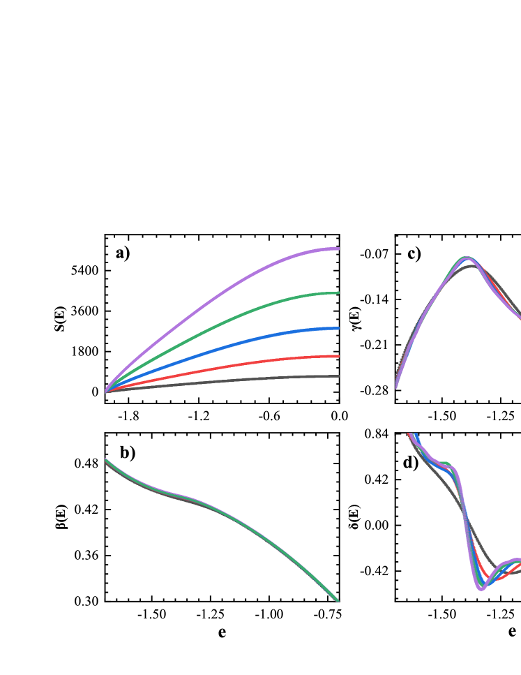
Figure 1: a) The logarithm of the density of states; b) the inverse temperature, $\beta(e)$; the first and the second derivatives of the inverse temperature, c) $\gamma(e)$ and d) $\delta(e)$ for the Ising model.

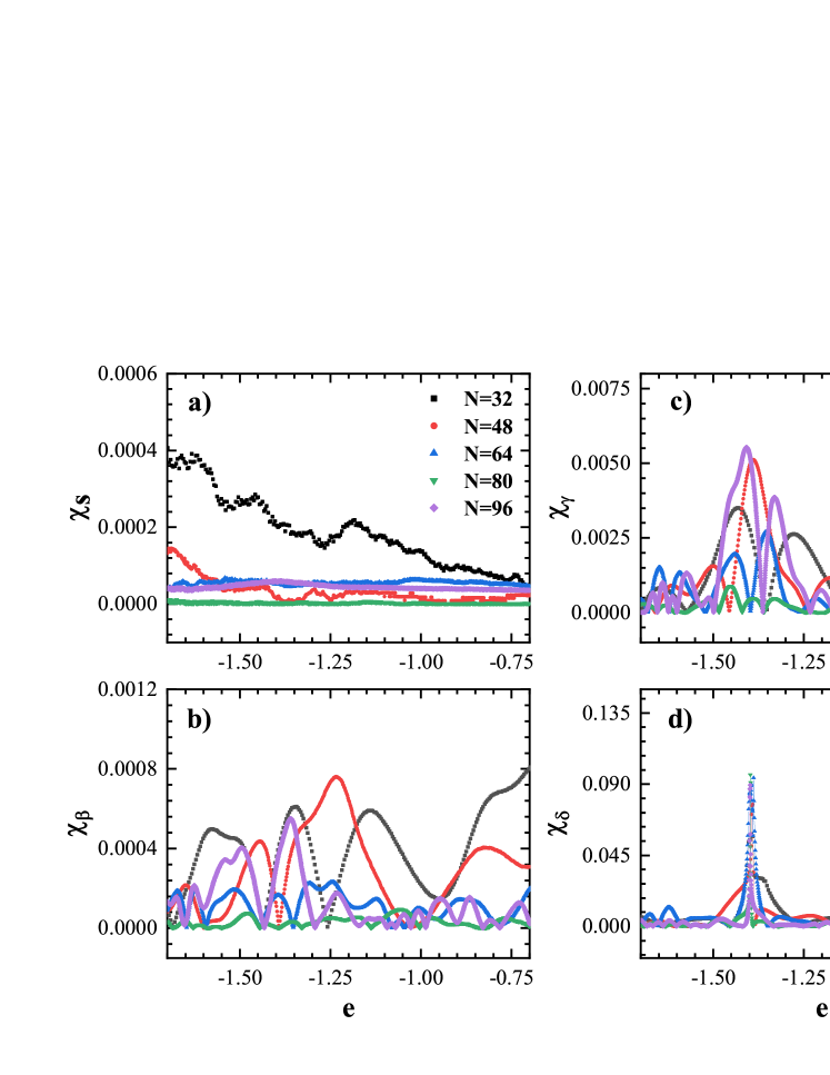
Figure 2: Relative errors of a) the logarithm of the DOSs; b) the inverse temperature, $\beta(e)$; the first and the second derivatives of the inverse temperature, c) $\gamma(e)$ and d) $\delta(e)$ for the Ising model.

The third dependent transition signals were detected as well. The curves for $\delta(E)$ had the negative maximums which could determine the third transition points. The points are shown in Table 3.

Table 3: Locations of the dependent third-order phase transitions for the Ising model.

$N$	32	48	64	96
$1/\beta$	2.727	2.597	2.554	2.540

The transition points obtained with the microcanonical and canonical methods coincide well and are in agreement with the results of Qi et al.’s work [9], which shows that it is reliable to perform microcanonical inflection-point analysis up to third-order transitions using the DOS obtained by the Wang–Landau sampling method.

3.2 Baxter-Wu model

The BW model in the triangular lattice has four degenerate ground states, and has a longer energy range for the spin-1 model. Hence, the simulated lattice sizes are from $N=30$ to $N=90$ for the spin-1/2 model and from $N=18$ to $N=60$ for the spin-1 model.

Using our obtained data on the DOS, we calculated the specific heat and analyzed the finite-size effect. The result we obtained is that the critical exponent $\alpha/\nu$ is equal to $1.022\pm 0.005$ for the spin-1/2 model, whereas it is equal to $1.120\pm 0.006$ for the spin-1 model. The spin-1/2 model belongs to the universality class of four-state Potts, of which the exponent nearly equals $1$. However, the exponent for the spin-1 model is larger than $1$, which suggests that the behavior of the thermodynamic limit of this model is nontrivial. Fig. 3 gives the finite-size effect and the energy distribution of the BW model. The double-peak distribution suggests the first-order transition. Besides, the distribution of spin-1/2 points at low energies shows ”random” behavior to some extent when lattice size is small. We emphasize here that the behavior does not come from simulation noise, and the behavior is not random. The DOS at low energy of this model results in the effect. Fig. 4. a) displays the DOS at $N=18$, and the error bars are too small to see. The DOS for spin-1/2 model shows the distinct non-smoothness, which may lead to the deterministic ”random” distribution.

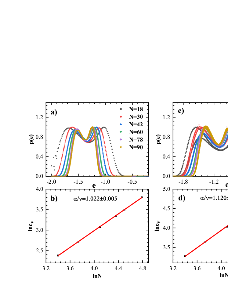
Figure 3: The probability distributions of the internal energy and the finite-size effect of the specific heat of the Baxter–Wu model: a), b) for spin-1/2, and c), d) for spin-1.

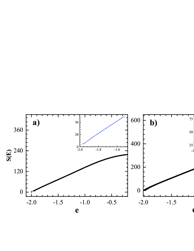
Figure 4: The DOSs of the BW model at lattice size $N=18$, a) for spin$-1/2$, b) for spin-1. The insets are the enlarged views of the low energy regions.

In contrast to the case of the spin-1/2 model, the distribution at a small lattice size for the spin-1 model shows two different height peaks at a low energy region. The DOS of $N=18$ (Fig. 4 . b)) for spin-1 model shows fluctuations that the number of the states at lower energy is larger than the states at nearest higher energy levels at the region of the low energy level, which gives rise to the two peaks. The reason for the unexpected phenomena is that square lattice adding next-nearest-neighbour diagonal bonds is used to produce a triangular lattice. The shape of this representation of triangular lattice is of a rhombus. As a result, for smaller lattice size, it can give rise to unexpected finite-size effect due to the different rotational symmetries from the real triangular lattice [32].

The microcanonical results for the spin-1/2 and spin-1 BW models are displayed in Fig. 5. The non-monotonic ”backbending” of the inverse temperature $\beta$, which is a typical signal of phase coexistence, is observed in both the spin-1/2 and spin-1 models. The positive maximum values of $\gamma$ reveal the first-order phase transitions of which the positions locate the transition points. As the lattice size increases, the values of $\gamma$ become smaller, implying the decrease in the ”latent heat”. This result is consistent with the results of the canonical analysis shown in Fig 3 a) and c).

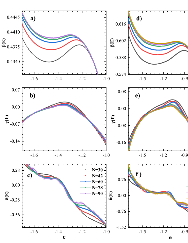
Figure 5: The inverse temperature $\beta(e)$, the first and the second derivatives of the inverse temperature $\gamma(e)$ and $\delta(e)$; a)–c) for spin-1/2, d)–f) for the spin-1 BW model.

Moreover, the signals of the third-order phase transitions appear in the curves of Fig. 5 c and f. Similar to the Ising model, both the independent and dependent transitions were detected. Some of the curves of $\delta(E)$ had positive minimums and negative maximums. However, if the lattice sizes are small, positive minimums and negative maximums of the curves may not appear. The behaviors are found in Ising model as well. The smaller system might show fourth-order phase transitions [9] which are hardly detected via Wang-Landau sampling data due to the simulation noises. Table 4 gives the locations of the third-order phase transitions. $\beta_{a,b}$ stands for the transition inverse temperature, where $a$ denotes the spin-1/2 or 1 models and $b$ denotes the type of transition. $d$ is for the dependent transition and $in$ is for the independent transition. NS stands for ”not simulated” and NF for ”not found”.

Table 4: Locations of the third-order transitions for the BW models.

$N$	18	24	30	42	48	60	78	90
$1/\beta_{1/2,d}$	NS	NS	NF	NF	NF	NF	NF	2.277
$1/\beta_{1/2,in}$	NS	NS	NF	NF	NF	NF	2.276	2.274
$1/\beta_{1,d}$	NF	NF	NF	NF	1.665	1.664	NS	NS
$1/\beta_{1,in}$	1.715	1.688	1.682	1.673	1.670	1.667	NS	NS

Due to the existence of the latent heat of the pseudo-first-order transitions, the higher-order phase transition shows some differences from the system with the second-order transition. The positions of the third-order independent phase transitions are at lower energy levels than the positions of the first-order phase transitions, whereas the positions of the dependent phase transitions are at higher energy levels. The inverse temperature $\beta$ has a non-monotonic ”backbending” phenomenon, and the locations of the third transitions are in the region of the backbending, which leads to the close positions between the independent and dependent transitions. In addition, the independent transitions refer to the transitions between the over-heated states with higher orders and the metastable states with low orders, whereas the dependent transitions might refer to the transitions between supercooled lower-order metastable states and the disordered states. The third-order phase transitions occur in the region of the coexisting phase, hence, the positions of the independent and dependent transitions are very close.

4 Conclusion

In summary, we used Wang–Landau sampling to obtain the DOSs for the Ising and BW models. Then, the orders of the pseudo-transitions for the finite-size systems were analyzed via the microcanonical inflection-point method. We also compared the microcanonical results with the canonical ones. The data for the Ising model reveal that the DOS obtained via Wang–Landau sampling can be used for analyzing the order of transitions up to the third order, and the positions of the second- and third-order transitions were precisely obtained. The differences of the phases below or above critical point were detected with the independent or dependent third-order pseudo-phase transitions which could not be observed via canonical methods. Based on the reliability of this method, we studied the spin-$1/2$ and -$1$ BW models. The data show that the finite-size BW models have the first and third transitions. The ”latent heat” of the first-order transitions decreases as the systems become larger in size. We conjecture that the ”latent heat” disappears at the thermodynamic limit. Third-order phase transitions in both the Ising and BW models imply the universality for the higher-order transitions to some extent. The dependent third order transitions occur at a higher energy than the corresponding independent transitions, which reveals that the systems would be in a less ordered phase before it goes into a ordered phase. This might have potential applications in materials science since dependent higher order transitions might help ones find the unstable structures. Consequently, it would be of importance to confirm the universality of the higher order phase transitions in different spin models and reveal the nature of transitions higher than the second order in future work.

5 Acknowledgements

We would like to thank Prof. Michael Bachmann for his valuable discussion and thank the anonymous referee for his/her helpful suggestions. This work is supported by the Natural Science Basic Research Program of Shaanxi (Program No.2022JM-039)

References

- [1] Pathria R K and Beale P D 2011 Statistical Mechanics, Third Edition (Academic, Boston)
- [2] Wilson K G 1983 Rev. Mod. Phys. 55 583
- [3] Brush S G 1967 Rev. Mod. Phys. 39 883
- [4] Landau D and Binder K 2021 A guide to Monte Carlo simulations in statistical physics (Cambridge university press)
- [5] Chamberlin R V 2015 Entropy 17 52–73
- [6] Chamberlin R V 2003 Phys. Lett. A 315 313–318
- [7] Newman M 2018 Networks (Oxford university press)
- [8] Gross D H 2001 Microcanonical thermodynamics: phase transitions in” small” systems (World Scientific)
- [9] Qi K and Bachmann M 2018 Phys. Rev. Lett. 120 180601
- [10] Qi K, Liewehr B, Koci T, Pattanasiri B, Williams M J and Bachmann M 2019 J. Chem. Phys. 150 054904
- [11] Beale P D 1996 Phys. Rev. Lett. 76 78
- [12] Sitarachu K, Zia R and Bachmann M 2020 J. Stat. Mech. 2020 073204
- [13] Wood D and Griffiths H 1972 J. Phys. C 5 L253
- [14] Baxter R and Wu F 1973 Phys. Rev. Lett. 31 1294
- [15] Baxter R J and Wu F 1974 Aust. J. Phys. 27 357–368
- [16] Schreiber N and Adler J 2005 J. Phys. A 38 7253
- [17] Liu W, Yan Z and Wang Y 2021 Commun. Theor. Phys. 73 015602
- [18] Antal T, Krapivsky P L and Redner S 2005 Phys. Rev. E 72 036121
- [19] Radicchi F, Vilone D, Yoon S and Meyer-Ortmanns H 2007 Phys. Rev. E 75 026106
- [20] Kargaran A and Jafari G 2021 Physical Review E 103 052302
- [21] Masoumi R, Oloomi F, Kargaran A, Hosseiny A and Jafari G 2021 Physical Review E 103 052301
- [22] Rabbani F, Shirazi A H and Jafari G 2019 Physical Review E 99 062302
- [23] Krawczyk M J and Kułakowski K 2021 Entropy 23 1418
- [24] Jorge L, Ferreira L and Caparica A 2020 Physica A 542 123417
- [25] Wang F and Landau D P 2001 Phys. Rev. Lett. 86 2050
- [26] Cunha-Netto A G d, Caparica A, Tsai S H, Dickman R and Landau D P 2008 Phys. Rev. E 78 055701
- [27] Vogel T, Li Y W, Wüst T and Landau D P 2013 Phys. Rev. Lett. 110 210603
- [28] Vogel T, Li Y W, Wüst T and Landau D P 2014 Phys. Rev. E 90 023302
- [29] Vogel T, Li Y W, Wüst T and Landau D P 2014 Exploring new frontiers in statistical physics with a new, parallel wang-landau framework J. Phys.: Conference Series vol 487 (IOP Publishing) p 012001
- [30] Vogel T, Li Y W and Landau D P 2018 A practical guide to replica-exchange wang—landau simulations J. Phys.: Conference Series vol 1012 (IOP Publishing) p 012003
- [31] Janke W 2002 Quantum Simulations of Complex Many-Body Systems: From Theory to Algorithms 10 423–445
- [32] Newman M E and Barkema G T 1999 Monte Carlo methods in statistical physics (Clarendon Press)