Finite-Key Analysis of Quantum Key Distribution with Characterized Devices Using Entropy Accumulation

Abstract

The Entropy Accumulation Theorem (EAT) was introduced to significantly improve the finite-size rates for device-independent quantum information processing tasks such as device-independent quantum key distribution (QKD). A natural question would be whether it also improves the rates for device-dependent QKD. In this work, we provide an affirmative answer to this question. We present new tools for applying the EAT in the device-dependent setting. We present sufficient conditions for the Markov chain conditions to hold as well as general algorithms for constructing the needed min-tradeoff function. Utilizing Dupuis’ recent privacy amplification without smoothing result, we improve the key rate by optimizing the sandwiched Rényi entropy directly rather than considering the traditional smooth min-entropy. We exemplify these new tools by considering several examples including the BB84 protocol with the qubit-based version and with a realistic parametric downconversion source, the six-state four-state protocol and a high-dimensional analog of the BB84 protocol.

1 Introduction

Quantum key distribution (QKD) protocols [1, 2] enable two legitimate parties (Alice and Bob) to establish shared secret keys in the presence of any eavesdropper (Eve) who has control over the channel connecting the two parties and is only limited by the laws of quantum mechanics. That is, QKD protocols establish an information-theoretically secure shared secret key. The generated secret keys can be used in many cryptographic applications that our modern cybersecurity relies on, such as encryption and authentication. The field of QKD has grown rapidly in the last couple decades. Novel protocols have been proposed and analyzed (see [3, 4, 5] for reviews). Many QKD experiments (e.g. [6, 7]) have been demonstrated to reach increasingly longer distances and/or to achieve higher key bits per second. The maturity of the field can be witnessed by development of commercial prototypes in several companies, successful launch of a QKD satellite in China [8], many ongoing efforts to launch QKD satellites from all over the world [9], and developments of chip-based QKD systems [10, 11, 12].

While currently the field of implementation security (as opposed to protocol security), requiring certification procedures and security proofs with more refined models, captures an increasing amount of attention, there are still challenges to be addressed on the level of protocol security itself. One major technical difficulty is guaranteeing security of the protocol when using finite resources. The security of a novel protocol is often first proved in the asymptotic key limit where Alice and Bob exchange infinitely many signals, since in that regime typically reduction to the identically and independently distributed (i.i.d.) assumption about the individual exchanged signals can be made and statistical fluctuations can be neglected. However, any realistic system can only exchange a finite number of signals. For example, the time interval of low orbiting satellites having line of sight to ground stations is limited to minutes, thus naturally limiting the total number of signals that can be exchanged. The study of security with finite resources is known as finite key analysis. In recent years, finite key analysis against general attacks has been performed for several QKD protocols. One aims to provide security proofs that allow one to generate the most key using the fewest signals and converge to the fundamental asymptotic limit quickly.

Over the past decade, several techniques have been proposed to bridge the gap between asymptotic security and finite key analysis against general attacks. The Quantum de Finetti theorem [13] was first used to achieve this task. While it makes no restrictions on the QKD protocol implemented, the key rate becomes very pessimistic at practical signal block size. The postselection technique [14] was later presented to improve the key rate if the protocol is permutation invariant with respect to any input. Although it gives better performance, the key rate is believed to remain pessimistic as it scales exponentially in the dimension of Alice and Bob’s signals. More recently, the entropy accumulation theorem [15, 16] was developed to offer tighter finite key analysis. It has been successfully applied to prove the security of device-independent (DI) QKD protocols [17, 18].

From the perspective of implementation security, DIQKD is favorable since it requires minimal assumptions on Alice and Bob’s devices and thus is immune to most side-channel attacks. Thanks to the entropy accumulation theorem [15] and its application to DIQKD [17], the experimental requirements to implement DIQKD have become within reach of state-of-the-art technologies. Very recently, proof-of-principle experimental demonstrations of DIQKD with positive key rates are reported for extremely short distances [19, 20, 21]. Even if the transmission distance is extended to practical regimes in a near future, a DIQKD system is expected to be more costly since the experimental requirements are still demanding. In fact beyond the experimental requirements, it may be viewed as significantly more expensive simply because at best one must use a new system of devices each time one wishes to establish a key because DIQKD is not known to be universally composably secure [22, 18]. As such, while DIQKD has advantages for implementation security and can be implemented, at least over very short distances, device-dependent QKD (i.e. QKD with characterized devices) remains the more practical option at the moment.

Beyond these limitations, as less assumptions are put on trusted parties’ devices, DIQKD key rates are unavoidably lower than a standard device-dependent QKD protocol. On the other hand, with the best practice to countermeasure known side-channel attacks, suitable risk management and use cases, and efforts from standardization, device-dependent QKD remains a vital player for a wide adoption of QKD in the future. Therefore, it is still of great interest to provide as tight as possible key rates for device-dependent QKD. Our goal here is to apply the entropy accumulation theorem to provide better finite key rates of device-dependent QKD.

So far, the entropy accumulation theorem has not been applied to determine the key rate for any device-dependent QKD protocol. There are two major obstacles to overcome in applying EAT to device-dependent QKD. The first one is to guarantee the Markov condition is satisfied by the protocol. This condition in effect guarantees the protocol is well-behaved in what side-information is leaked to Eve during the protocol. This is an important aspect as device-dependent protocols often make use of announcing more information about each signal than DI protocols. In this work, we provide sufficient conditions for satisfying the Markov conditions of the EAT. Specifically, we prove that when Alice and Bob’s announcements are determined by POVMs with a simple block-diagonal structure, then the protocol satisfies the Markov chain conditions (see Section 4.2). This block-diagonal structure is satisfied for many practical discrete-variable QKD protocols. The second challenge is to have a general method to construct the required min-tradeoff function. This challenge has been addressed for the device-independent scenario in a recent work [23], but has not been addressed in the device-dependent scenario in which we have more structure of which to take advantage. We present a numerical method (with two algorithm variants) to construct tight min-tradeoff functions for device-dependent QKD protocols satisfying the above restrictions. The basic idea of one of the algorithm variants is similar to our existing numerical method for asymptotic key rates [24, 25] and the other one which improves on the first one is based on the Fenchel duality. However, unlike the formulation of the objective function in Refs. [24, 25], we present here a different formulation of the objective function for the optimization which has advantages in terms of dimension needed for the numerical optimization as well as a simpler representation of procedures to handle classical postprocessing. Using the guarantee of our numerical method constructing a min-tradeoff function, we present a general key length bound. It is largely similar to that of Ref. [17], but, building on the recent result that privacy amplification may be characterized using sandwiched Rényi entropies rather than the smooth min-entropy [26], we are able to show we can improve the key rate by optimizing over sandwiched Rényi entropies rather than using the smooth min-entropy bounds. We then apply our method to several examples. The first example is a simple qubit-based BB84 protocol and the second example is the entanglement-based six-state four-state protocol [27]. We use these two examples to demonstrate behaviors of our algorithms. The third one is a high-dimensional analog of the BB84 protocols. We compare these results with the key rates obtained by the postselection technique [14] to show that the EAT can outperform the postselection technique for high-dimensional signals. In the last example, we demonstrate that our method can also work for optical implementations of QKD and in particular, we study the entanglement-based BB84 protocol with a spontaneous parametric downconversion source in a lossy and noisy channel.

Our work here provides a first step along the direction of applying EAT to general device-dependent QKD protocols. Currently, we limit ourselves to entanglement-based protocols. To handle prepare-and-measure protocols, one needs to be able to incorporate the source-replacement scheme [28] into the EAT subprotocol and to be able to add a promise that Alice’s reduced density operator is not affected by Eve’s attacks. There remain technical challenges to do so. We leave this for future work.

The rest of the paper is organized as follows. In Section 2.1, we summarize our notational conventions and in Section 2.2, we review the security definition of QKD. In Section 3, we review the entropy accumulation theorem and adapt the theorem to the device-dependent setting. We do this first in the case where side information is all seeded randomness, as was the case in previous works. We then provide sufficient conditions for satisfying the Markov chain conditions necessary to apply the EAT without relying on all side-information being randomly seeded. This is important as many device-dependent QKD protocols make announcements which depend on the outcome of the measurement. In Section 4, we describe the generic protocol to which our method is applicable and also the assumptions on public announcements. In Section 5, we then apply the EAT to this family of protocols and obtain a key length formula. In Section 6, we discuss how to construct min-tradeoff functions numerically and present two numerical algorithms for obtaining a nearly tight min-tradeoff function. In Section 7, we apply our method to several examples. We then conclude in Section 8. We leave technical details to appendixes.

2 Preliminaries

We discuss the notational convention and some useful definitions in Section 2.1. We then review the security definition of QKD in Section 2.2.

2.1 Notation

We briefly summarize the notation which we use throughout this work.

Table 1: Overview of notational conventions.

General notations	Descriptions
$A,B,C,\cdots$	Quantum systems and their associated Hilbert spaces
$|A|,|B|,|C|,\cdots$	Dimension of the Hilbert spaces
$A^{n}_{1}$	Shorthand for $A_{1}A_{2}\cdots A_{n}$
$[n]$	The set of natural numbers from 1 to $n$
$\id$	Identity map
$f$	A min-tradeoff function
$\bm{f}$	A vector that is used to construct the min-tradeoff function $f$
$\bm{1}$	A vector of all ones
EAT statement	Descriptions
$P_{i}$	Public information in the EAT statement
$S_{i}$	Secret information in the EAT statement
$T_{i}$	Test flag variable
$X_{i}$	Test result register in the EAT statement
$E$	Eve’s system
$\Omega$	An event
$\rho[\Omega]$	Probability of $\Omega\subset\mathcal{X}$ for $\rho_{XA}$ (See main text in Section 2.1)
$\mathsf{freq}($)	Frequency of a given event
$\bm{q}$	A probability vector
${{\mathbb{P}}}(\mathcal{X})$	The probability vector space with events from $\mathcal{X}$
$\mathrm{D}(A)$	The set of quantum states on Hilbert space $A$

For consistency, we at times use the notation for quantum states conditioned on an event from previous works [15, 16]. Let $\mathcal{X}$ be a finite alphabet, $X\cong\mathbb{C}^{|\mathcal{X}|}$. Then a classical-quantum (CQ) state may be written as $\rho_{XA}=\sum_{x\in\mathcal{X}}\outerproduct{x}{x}\otimes\rho_{A,x}$ where the quantum part of this decomposition is generally called the conditional state. Given an event $\Omega\subset\mathcal{X}$, the probability of the event is $\rho[\Omega]$, which may be calculated by $\rho[\Omega]:=\sum_{x\in\Omega}\Tr[\rho_{A,x}]$. Lastly, the state conditioned on the event is given by $\rho_{XA|\Omega}=\frac{1}{\rho[\Omega]}\sum_{x\in\Omega}\rho_{A,x}$. Note that a conditioned state is therefore re-normalized.

We will also require various entropies which we also introduce here. We use the notation of [15, 16]. We refer to [29] for further background, but note that the notation differs in that work.

For $\alpha\in(0,1)\cup(1,\infty)$, define the minimal divergence by

$$D_{\alpha}(\rho||\sigma):=\begin{cases}\frac{1}{\alpha-1}\log\frac{\|\sigma^{\frac{1-\alpha}{2\alpha}}\rho\sigma^{\frac{1-\alpha}{2\alpha}}\|^{\alpha}_{\alpha}}{\Tr(\rho)}&\text{ if }\alpha<1\text{ or if }\alpha>1\text{ and }\mathrm{supp}(\rho)\subseteq\mathrm{supp}(\sigma)\\ +\infty&\text{ otherwise}\end{cases}\ ,$$

where $\norm{\cdot}_{p}$ is the Schatten $p$-norm for $p\geq 1$ and the definition is extended to all $p>0$. For any $\rho\in\mathrm{D}(A\otimes B)$, $\sigma\in\mathrm{D}(B)$, define

$$H_{\alpha}(\rho_{AB}||\sigma_{B}):=-D_{\alpha}(\rho_{AB}||\mathbb{1}_{A}\otimes\sigma_{B})\,.$$

We then define $H_{\alpha}(A|B)_{\rho_{AB}}:=H_{\alpha}(\rho_{AB}||\rho_{B})$ and $H^{\uparrow}_{\alpha}(A|B)_{\rho}:=\sup_{\sigma_{B}}-D_{\alpha}(\rho_{AB}||\mathbb{1}_{A}\otimes\sigma_{B})$. We refer to both these classes of entropies as sandwiched Rényi entropies. We may also recall the smooth min-entropy defined by

$$H^{\varepsilon}_{\min}(A|B)_{\rho_{AB}}:=\underset{\tilde{\rho}\in\mathcal{B}^{\epsilon}(\rho_{AB})}{\max}H_{\min}(A|B)_{\tilde{\rho}}\ ,$$

where $H_{\min}(A|B)_{\rho_{AB}}:=-\log(\min\{\Tr(Y): \rho_{AB} \leq\mathbb{1}_{A} \otimes Y_{B} \ \})$, $\mathcal{B}^{\epsilon}(\rho_{AB}):=\{\tilde{\rho}_{AB}\geq 0:\Tr(\tilde{\rho}_{AB})\leq 1\,\&\,P(\tilde{\rho}_{AB},\rho_{AB})\leq\varepsilon\}$, and $P$ is the purified distance [30, 29]. Throughout this work, $\log$ is referred to $\log_{2}$.

2.2 QKD security definition

We provide a short review of the $\varepsilon$-security framework of QKD [13, 31]. A QKD protocol is $\varepsilon$-secure if for any input state, the output state $\rho_{S_{A}S_{B}E}$ conditioned on that the protocol does not abort (and thus subnormalized) satisfies

$$\frac{1}{2}\norm{\rho_{S_AS_BE}-\pi_{S_AS_B}\ox\rho_E}_{1}\leq\varepsilon\,,$$ (1)

where $\pi_{S_{A}S_{B}}=\sum_{s\in\mathcal{S}}\frac{1}{\absolutevalue{\cS}}\outerproduct{s}{s}\otimes\outerproduct{s}{s}$, and $\mathcal{S}$ is the space of keys that could be generated from the protocol. The security parameter $\varepsilon$ quantifies the amount of deviation of the real protocol from an ideal protocol. In an ideal QKD protocol, Alice and Bob are supposed to obtain an identical key, which is the correctness requirement; The key is supposed to be distributed from a uniform distribution among all possible keys and that Eve knows no information about the key, which is the secrecy requirement. This security definition in terms of trace distance has an operational interpretation: If a distinguisher is given either the real or the ideal protocol as a black box with an equal a priori probability and the goal is to verify which protocol the black box implements, then the probability that this distinguisher can guess correctly by looking at output states of the black box is at most $\frac{1}{2}(1+\varepsilon)$. We note that in the case of aborting, both protocols output a trivial key symbol.

In Equation 1, we use subnormalized states. Equivalently, if we define in terms of normalized output states $\tilde{\rho}_{S_{A}S_{B}E}=\rho_{S_{A}S_{B}E}/\Tr(\rho_{S_AS_BE})$ and $\tilde{\rho}_{E}=\rho_{E}/\Tr(\rho_E)$ where $\Tr(\rho_{S_AS_BE})=\Tr(\rho_E):=\Pr(\text{accept})$ denotes the probability that the protocol does not abort, then Equation 1 can be written as

$$\frac{1}{2}\Pr(\text{accept})\norm{\tilde{\rho}_{S_AS_BE}-\pi_{S_AS_B}\ox\tilde{\rho}_E}_{1}\leq\varepsilon\ .$$ (2)

It is often convenient to discuss the secrecy requirement and correctness requirement separately since the correctness requirement is usually guaranteed by the error correction and error verification steps of a QKD protocol. A key is $\varepsilon_{\text{\rm sec}}$-secret if

$$\frac{1}{2}\norm{\rho_{S_AE}-\pi_{S_A}\ox\rho_E}_{1}\leq\varepsilon_{\text{\rm sec}}\,,$$ (3)

where $\pi_{S_{A}}=\sum_{s\in\mathcal{S}}\frac{1}{\absolutevalue{\cS}}\outerproduct{s}{s}$. A QKD protocol is $\varepsilon_{\text{cor}}$-correct if the joint probability that the protocol does not abort and that Bob’s key is different from Alice’s key is at most $\varepsilon_{\text{cor}}$. By the triangle inequality of the trace norm, it is easy to see that if the QKD protocol is $\varepsilon_{\text{cor}}$-correct and it generates $\varepsilon_{\text{\rm sec}}$-secret keys, then the protocol is $\varepsilon$-secure with $\varepsilon=\varepsilon_{\text{\rm sec}}+\varepsilon_{\text{cor}}$.

3 The Entropy Accumulation Theorem

Figure 1: Diagrammatic depiction of EAT process and theorem. (a) Captures the overall process and (b) is the process captured by the min-tradeoff function (See Definition 2). They are related by the Entropy Accumulation Theorem (Theorem 1). Note that $\mathcal{M}_{n}$ may be viewed as outputting a trivial register, $R_{n}\cong\mathbb{C}$, which we have suppressed. The output of the EAT process is $\rho_{S^{n}_{1}P^{n}_{1}X^{n}_{1}E}$, the output registers along with the purification.

In this section we review the Entropy Accumulation Theorem (EAT) [15, 16] which is the unifying technical tool of this work. The EAT is motivated as follows. Fundamentally, the formal property of secrecy using a process with a finite number of rounds is characterized by the smooth min-entropy [13]. Unfortunately, the smooth min-entropy is a functional that is difficult to calculate directly for large systems. It therefore follows that one wishes to determine tight bounds on the smooth min-entropy of a given process via a reduction that is computationally feasible. The EAT accomplishes this task for well-behaved sequential processes. The idea of the EAT is that, under some reasonable behavior, one can bound the smooth min-entropy of the finite-length process by the worst-case accepted asymptotic behavior along with some correction terms.

However, in this work we find empirically that a recent work that characterizes secrecy using the sandwiched Rényi entropies $H^{\uparrow}_{\alpha}$ [26] can lead to improved key rates. As such, rather than presenting results in terms of smoothed entropies in the main text, we present them in terms of $H^{\uparrow}_{\alpha}$ entropies. For completeness and perhaps intuition, in Appendix D, we present all results in terms of smooth entropies. We now present the formal statement of the EAT along with relevant definitions after which we elaborate on the intuition and relation to the rest of this work.

3.1 Formal statement

To formally state the EAT, we review some definitions first [15, 16] (See Figure 1 for a visualization).

Definition 1 (EAT Channels).

EAT channels are Completely Positive Trace-Preserving (CPTP) maps

$$\mathcal{M}_{i}:R_{i-1}\to S_{i}P_{i}X_{i}R_{i}$$ (4)

where for all $i\in\{1,\cdots n\}$, $R_{i}$ are quantum systems (with $R_{n}\cong\mathbb{C}$ the trivial register) and where $S_{i}$, $P_{i}$, and $X_{i}$ for $i\in\{1,\cdots n\}$ are classical systems taking values in $\mathcal{S},\mathcal{P}$, and $\mathcal{X}$ respectively.

Furthermore, we assume that $X_{i}$ is a deterministic function of $S_{i}$ and $P_{i}$. In other words, the EAT channels can be decomposed as

$$\mathcal{M}_{i}=\mathcal{T}_{i}\circ\mathcal{M}_{i}^{\prime}$$ (5)

where $\mathcal{M}_{i}^{\prime}:R_{i-1}\to S_{i}P_{i}R_{i}$ is some CPTP map and where $\mathcal{T}_{i}:S_{i}P_{i}\to S_{i}P_{i}X_{i}$ is a classical operation assigning a value for $X_{i}$ as a function of $S_{i}$ and $P_{i}$ of the form

$$\mathcal{T}_{i}(W_{S_{i}P_{i}})=\sum_{s\in\mathcal{S},\;p\in\mathcal{P}}(\Pi_{S_{i},s}\otimes\Pi_{P_{i},p})W_{S_{i}P_{i}}(\Pi_{S_{i},s}\otimes\Pi_{P_{i},p})\otimes\ket{t(s,p)}\bra{t(s,p)}_{X_{i}},$$ (6)

where $\{\Pi_{S_{i},s}:s\in\mathcal{S}\}$ and $\{\Pi_{P_{i},p}:p\in\mathcal{P}\}$ are families of mutually orthogonal projectors on $S_{i}$ and $P_{i}$, and the function $t:\mathcal{S}\times\mathcal{P}\to\mathcal{X}$ is a deterministic function.

In the above definition, the registers $S_{i}$ and $P_{i}$ stand for ‘secret’ key registers and ‘public’ announcement registers respectively as this will be the natural interpretations of these registers in the context of cryptography. The $X_{i}$ register is then a ‘testing’ register which is a function of the secret and public registers. Note that we consider the particular case of classical systems $S_{i}$ and $P_{i}$, compared to [15, 16, 26] where they can be quantum, as this is sufficient for this work. The main idea of the EAT channels is that they can be composed such as in Figure 1, starting from an initial state $\rho_{R_{0}E}^{0}\in\mathrm{D}(R_{0}\otimes E)$ and applying the EAT maps sequentially to produce the output state

$$\rho_{S^{n}_{1}P^{n}_{1}X^{n}_{1}E}=(\mathcal{M}_{n}\circ\cdots\circ\mathcal{M}_{1}\otimes\id_{E})(\rho_{R_{0}E}^{0})\,.$$ (7)

The most important restriction on this state is that we require it to satisfy the Markov chain conditions:

$$S_{1}^{i-1}\leftrightarrow P_{1}^{i-1}E\leftrightarrow P_{i}\qquad\forall i\in\{1,\ldots,n\}\ ,$$ (8)

where one may recall a quantum Markov chain, denoted $A\leftrightarrow B\leftrightarrow C$, is a quantum state $\rho_{ABC}$ such that the conditional mutual information is zero, i.e. $I(A:C|B)=0$. It follows the Markov chain conditions are claims about the mutual information between the previous secret registers and the previous public registers (along with Eve’s information) when conditioned on the current public announcement. The reason this is important to the proof of the theorem is that the Markovian behavior restriction guarantees that the process (defined by the sequential application of $\mathcal{M}_{i}$) does not a priori destroy entropy being accumulated in the $S^{n}_{1}$ registers. It does this by guaranteeing that, for each $i\in[n]$, the public announcement in round $i$, $P_{i}$, is not correlated to the generated secret information of previous rounds, $S^{i-1}_{1}$, when we condition on the side information $E$ and all public announcements up to then $P_{1}^{i-1}$.

It is also perhaps useful to preemptively stress that the EAT channels do not have to be a model of the actual implementation, rather they only need to capture the same relationships between the output random variables $S^{n}_{1},P^{n}_{1}$ and $X^{n}_{1}$ as the actual implementation because the entropy only depends on the random variables. This insight is what allowed the EAT to be used for device-independent information processing where dimensions cannot be bounded.

Definition 2 (Min-tradeoff functions).

An affine function $f$ on the space of probability distributions ${{\mathbb{P}}}(\mathcal{X})=\{\bm{p}\in\mathbb{R}^{\absolutevalue{\cX}}:\bm{p}(x)\geq 0,\sum_{x}\bm{p}(x)=1\}$ is called a min-tradeoff function for the EAT channel $\mathcal{M}_{i}$ if it satisfies

$$f(\bm{q})\leq\min_{\nu\in\Sigma_{i}(\bm{q})}H(S_{i}|P_{i}R)_{\nu}\quad\forall\bm{q}\in{{\mathbb{P}}}(\mathcal{X}),$$ (9)

where the minimization is over the set of quantum states compatible with the statistics $\bm{q}$ that is defined as below:

$$\Sigma_{i}(\bm{q}):=\left\{\nu_{S_{i}P_{i}X_{i}R_{i}R}=(\mathcal{M}_{i}\otimes\id_{R})(\omega_{R_{i-1}R}):\omega\in\DM(R_{i-1}\otimes R)\text{ and }\nu_{X_{i}}=\bm{q}\right\}\,,$$ (10)

where $R$ is isomorphic to $R_{i-1}$.

Remark 1.

Note that Ref. [15] considers affine functions. However, because of $\sum_{x}\bm{q}(x)=1$, any affine function on ${{\mathbb{P}}}(\mathcal{X})$ can be represented as a linear function. In particular, $f$ can be specified by a vector $\bm{f}\in\mathbb{R}^{\absolutevalue{\cX}}$, that is, $f(\bm{q})=\bm{f}\cdot\bm{q}:=\sum_{x}\bm{f}(x)\bm{q}(x)$. We note that this is equivalent to an affine function since for an affine function $f^{\prime}_{0}+\bm{f^{\prime}}\cdot\bm{q}$, one can define $\bm{f}(x)=\bm{f^{\prime}}(x)+f^{\prime}_{0}\ \forall x\in\mathcal{X}$ such that $f^{\prime}_{0}+\bm{f^{\prime}}\cdot\bm{q}=\bm{f}\cdot\bm{q}$.

By Definition 2, the min-tradeoff function characterizes the minimum amount of (von Neumann) entropy of the secret information conditioned on the public information and quantum side-information (encoded as the register $R$) for all probability distributions on the testing register. This encapsulates the notion of the minimum von Neumann entropy being accumulated in a given round. For QKD security proofs, the min-tradeoff function can be seen as the term that bounds Eve’s ignorance about the key in the asymptotic regime given by the Devetak-Winter formula [33], and so the min-tradeoff function may be seen as determining the first-order term in a finite-size key distillation protocol.

With these considerations, we can state the EAT with its improved second order term [16].

Theorem 1 (Special Case of Proposition V.3 of [16]).

Consider EAT channels $\mathcal{M}_{1},...,\mathcal{M}_{n}$ and their output $\rho_{S^{n}_{1}P^{n}_{1}X^{n}_{1}E}$ such that it satisfies the Markov conditions and $S_{i}$ is a classical register for all $i\in[n]$. Let $h\in\mathbb{R}$, $\alpha\in(1,2)$, and $f$ be a min-tradeoff function for $\mathcal{M}_{1},\dots,\mathcal{M}_{n}$. Then, for any event $\Omega\subseteq\mathcal{X}^{n}$ that implies $f(\mathsf{freq}(X_{1}^{n}))\geqslant h$,

$$H_{\alpha}^{\uparrow}(S_{1}^{n}|P_{1}^{n}E)_{\rho_{|\Omega}} >nh-n\frac{(\alpha-1)\ln 2}{2}V^{2}-\frac{\alpha}{\alpha-1}\log\frac{1}{\rho[\Omega]}-n(\alpha-1)^{2}K_{\alpha}$$ (11)

holds for

$$V =\sqrt{\mathsf{Var}(f)+2}+\log(2 d_{S}^{2}+1)\;$$ (12)

$$K_{\alpha} =\frac{1}{6(2-\alpha)^{3}\ln 2}2^{(\alpha-1)(\log d_{S}+(\mathsf{Max}(f)-\mathsf{Min}_{\Sigma}({f})))}\ln^{3}\left(2^{\log d_{S}+(\mathsf{Max}(f)-\mathsf{Min}_{\Sigma}(f))}+e^{2}\right)$$ (13)

where

$$\mathsf{Max}(f) :=\max_{\bm{q}\in{{\mathbb{P}}}(\mathcal{X})}f(\bm{q}),$$ (14)

$$\mathsf{Min}(f) :=\min_{\bm{q}\in{{\mathbb{P}}}(\mathcal{X})}f(\bm{q}),$$

$$\mathrm{Min}_{\Sigma}(f) :=\min_{\bm{q}:\Sigma_{i}(\bm{q})\neq\emptyset}f(\bm{q}),$$

$$\mathrm{Var}(f) :=\max_{\bm{q}:\Sigma_{i}(\bm{q})\neq\emptyset}\sum_{x}\bm{q}(x)\bm{f}(x)^{2}-\left[\sum_{x}\bm{q}(x)\bm{f}(x)\right]^{2}$$

and $d_{S}=\max_{i\in[n]}|S_{i}|$ is the maximum dimension of the systems $S_{i}$.

Remark 2.

Note that, beyond the Markov chain conditions, the EAT applying to a state depends on the event $\Omega\subseteq\mathcal{X}^{n}$ implying $f(\mathsf{freq}(X^{n}_{1}))$. Letting $\mathcal{Z}$ be a finite alphabet, if one is interested in an event $\Omega^{\prime}\subseteq\mathcal{Z}^{n}\times\mathcal{X}^{n}$ that guarantees such an $\Omega$ (i.e. $\Pr[\Omega|\Omega^{\prime}]=1$ which denotes the probability of event $\Omega$ conditioned on event $\Omega^{\prime}$) then, assuming the conditions for EAT held on generating $X^{n}_{1},S^{n}_{1},P^{n}_{1}$, the EAT will hold for $\rho_{X^{n}_{1}S^{n}_{1}P^{n}_{1}E|_{|\Omega^{\prime}}}$. This has been used implicitly in previous works such as [17], but we stress it here for completeness as we also use it.

It is worth noting the above theorem from [16] is actually an improved version of the original EAT [15]. The improvement is in the the second-order term where the dependency on the gradient of the min-tradeoff function $f$ is eliminated, which for certain applications caused the second-order term to dominate. We note that for a specific choice of $\alpha$, one can write Equation 11 in the form $H_{\alpha}^{\uparrow}>nh-O(\sqrt{n})$ [16] to clearly separate the first-order and second-order terms. However, we do not state it in this form because, while asymptotically optimal, to get the best finite size bounds we will optimize over the parameter $\alpha\in(1,2)$ as suggested in [16]. It is also noted that the exact from of the expression of $K_{\alpha}$ here uses the fact that $S_{i}$ is classical [16, Dicussion after Eq. (22)].

3.2 Applying EAT to device-dependent QKD

3.2.1 Tensor product structure

As noted earlier, the EAT maps in general do not have to be the same maps as the actual process as long as they capture the same relationship between output random variables. In the case of device-independent information processing, this is necessary since one cannot describe the device itself. In contrast, for device-dependent QKD as we consider here, without loss of generality we can let the EAT maps model the guaranteed behavior of the device in each round. It then follows that the EAT maps act on separate quantum systems. Formally, if we let $(Q_{i})_{i\in[n]}$ be $n$ quantum systems then we can consider the $n$ rounds of the QKD protocol as $n$ CPTP maps of the form

$$\widetilde{\mathcal{M}}_{i}:Q_{i}\rightarrow S_{i}P_{i}X_{i}\,,$$ (15)

each acting independently on its own $Q_{i}$ space. It follows that these maps can be expressed in the notation of the EAT theorem by defining the EAT channels $\mathcal{M}_{i}:R_{i-1}\rightarrow S_{i}P_{i}X_{i}R_{i}$ as follows:

$$\mathcal{M}_{i} =\widetilde{\mathcal{M}}_{i}\otimes\id_{Q_{i+1}^{n}}$$ (16)

where $R_{i}=\bigotimes_{j=i+1}^{n}Q_{j}$ and $\id_{Q_{i+1}^{n}}$ is the identity map on the registers $Q_{i+1}^{n}$. In other words, at round $i$ the EAT channel $\mathcal{M}_{i}$ effectively only acts on the system $Q_{i}$ to produce the outputs $S_{i},P_{i},$ and $X_{i}$, but not on the next systems $Q_{i+1}^{n}$.

By the fact that the outputs $S_{i}$ and $P_{i}$ are classical, we can make another simplification. In this case, the first requirement in Definition 1 of the EAT channels boils down to the requirement that $X_{i}$ is obtained by applying a deterministic function on $S_{i}$ and $P_{i}$: $x_{i}=t(s_{i},p_{i})$. In typical QKD protocols, we can further assume this function is identical for all rounds. Under this assumption, the EAT channels are thus entirely defined by specifying the function $t$ and the POVM elements $\{M_{sp}\}_{s,p}$ such that

$$\widetilde{\mathcal{M}}_{i}(\rho)=\sum_{s,p}\Tr(\rho M_{sp})\outerproduct{s,p}{s,p}_{S_{i}P_{i}}\otimes\outerproduct{t(s,p)}{t(s,p)}_{X_{i}}$$ (17)

for all $\rho\in\mathrm{D}(Q_{i})$. These POVM elements $\{M_{sp}\}_{s,p}$ are uniquely associated to $\widetilde{\mathcal{M}}_{i}$ and satisfy $M_{sp}\geq 0$ and $\sum_{s,p}M_{sp}=\idm{}$.

Now that we have reduced the scope of the EAT theorem, we still have two challenges to solve. The first challenge is how we can generate the best possible min-tradeoff function. The second is how we guarantee the Markov chain conditions in Equation 8.

3.2.2 Challenge 1: constructing optimal min-tradeoff functions

It is desirable to have a general procedure (applicable to many protocols) to construct min-tradeoff functions according to Definition 2. In addition to having valid min-tradeoff functions, we would like to find the best possible min-tradeoff function that can produce as tight key rates as possible for each signal block size when it is used in the EAT. In general, the construction of tight min-tradeoff functions is difficult. The difficulty arises from the non-trivial behavior of the conditional von Neumann entropy of the output state of a map (in this case the EAT channel) as a function of the resulting observations. We note that while for certain small-dimensional and theoretically simple QKD protocols, it may be possible to determine the optimal min-tradeoff function from uncertainty relations [15, Section 5.1], the analytic construction of min-tradeoff functions for generic device-dependent protocols is less straightforward, and thus it warrants a numerical method. This issue has also been recognized in the device-independent scenario and been addressed with its own numerical method [23]. In this work, we address this issue in the device-dependent setting and utilize additional structures of device-dependent QKD protocols. In Section 6, we present two algorithms for numerically constructing (almost) tight min-tradeoff functions in the case where one knows the structure of the EAT channels.

3.2.3 Challenge 2: guaranteeing Markov chain conditions

The Markov chain conditions [Equation 8] put strong restrictions on the maps $\mathcal{M}_{i}$’s that can be used with the EAT theorem. Roughly speaking, it states that, from the point of view of the adversary $E$, the process at round $j$ does not leak information about the secret register(s) $S_{i}$ of previous rounds $i<j$. In typical device-independent protocols, this restriction on the output state is in a sense trivially satisfied as all public announcements $P_{i}$, such as measurement settings, are independently seeded with random numbers. In other words, the probability distribution of the announcement $P_{i}$ does not depend on the state sent by Eve. Formally, if $\{p\}$ is the set of public announcements in round $i$ and there are $n$ rounds, then the Markov chain conditions trivially hold if $\Pr[p|\rho_{i}]=\Pr[p]$ $\forall\rho_{i}\in\mathrm{D}(Q_{i})$, $\forall i\in[n]$, i.e., the distribution over announcements is independent of the state being measured in each round.

However, one advantage of device-dependent QKD over device-independent QKD is its ability to have more complicated public announcement structures. One example is postselection on detection events in device-dependent QKD. Postselection implicitly requires an announcement. However, since the probability of a detection event depends on the state sent by Eve, the public announcement is not based on independently seeded randomness. A simple argument shows that this is potentially problematic, as it can lead to a violation of the Markov chain conditions, even when the EAT channels act on independent systems. This happens when Eve prepares a pure state $\ket{\phi}_{Q_{1}^{n}E}=\ket{\psi}_{Q_{1}^{n}}\otimes\ket{\psi^{\prime}}_{E}$, entangled between different rounds but not with her quantum memory. In that case, there can be correlations between announcements in one round and the private key register in another round. This could potentially prevent us from applying the EAT even if Eve could only learn from the public announcement. We therefore prove in Appendix A that the following condition (Definition 3) still guarantees the Markov conditions hold for Eve’s optimal attack, which is sufficient for applying the EAT (Theorem 1). We state this result below as Theorem 2.

Definition 3.

Given some quantum-to-classical CPTP map $\mathcal{W}:Q\rightarrow SP$ which can be fully specified by a POVM $\{M_{sp}:s\in\mathcal{S},\ p\in\mathcal{P}\}$, we say that the variable $P$ is weakly dependent (on the input state) when there exists a decomposition of the input space $Q$ into a direct sum of orthogonal subspaces $V^{\lambda}$, i.e., $Q=\bigoplus_{\lambda}V^{\lambda}$, such that

1. the channel $\mathcal{W}$ is block diagonal along $V^{\lambda}$: i.e., its POVM elements are of the form $M_{sp}={\bigoplus}_{\lambda}M_{sp}^{(\lambda)}$ with $M_{sp}^{(\lambda)}\in\mathcal{L}(V^{\lambda})$ acting on $V^{\lambda}$;

2. the probability of an announcement $P$ is the same for all states in a given subspace $V^{\lambda}$: i.e., there exist constants $c_{p,\lambda}$’s such that

   $$\mathrm{Pr}_{P}(p|\rho_{\lambda})=c_{p,\lambda}\,,\quad\text{ for all }\rho_{\lambda}\in D(V^{\lambda})$$ (18)

   where $\mathrm{Pr}_{P}(p|\rho_{\lambda}):=\Tr[M_{p}\rho_{\lambda}]$ with $M_{p}=\sum_{s}M_{sp}$.

Note that (b) in the definition is equivalent to saying that for each $\lambda$ and $p$, $M_{p}^{(\lambda)}:=\sum_{s}M_{sp}^{(\lambda)}=c_{p,\lambda}\idm_{V^{\lambda}}$ is proportional to the identity. This means that, equivalently, for any $\sigma\in Q$, $\Pr_{P}(p|\sigma)=c_{p,\lambda}\Tr[\Pi_{\lambda}\sigma\Pi_{\lambda}]$, where $\Pi_{\lambda}$ is the projector onto the subspace, i.e. the announcement only depends on a constant and the weight of the state on the subspace, which makes it ‘weakly’ dependent on the state. For intuition, this is distinct from independently randomly seeded announcements where each announcement has POVM elements of the form $M_{p}=c_{p}\idm_{Q}$, which results in the announcement being independent on the state all together. Note the independently randomly seeded case trivially satisfies Definition 3, and so it is a (strictly) special case of weakly dependent announcements.

Here we state that the advantage of weakly dependent announcements is that they guarantee the EAT may be applied.

Theorem 2.

If the announcements $P_{i}$ of the CPTP maps $\widetilde{\mathcal{M}}_{i}:Q_{i}\rightarrow S_{i}P_{i}X_{i}$ are weakly dependent, then the result of Theorem 1 may be applied to prove security.

We give a physical intuition why this theorem would hold and defer the proof to Appendix A. The POVM being of the block-diagonal form in Definition 3 means the subspace information is knowable to Eve. This is because without loss of generality, Eve should send such block-diagonal states and so she knows the information by implementing a quantum nondemolition (QND) measurement that determines the subspace which she then stores in a secondary register. Indeed, this idea of Eve having an extra register with the subspace information is how this is proven in Appendix A. We note equivalently that Eve’s purification of such a block-diagonal state includes the subspace information and so it is knowable to Eve from the perspective of purification as well.

4 The Quantum Key Distribution Protocol

In this section we present the class of entanglement-based (EB) QKD protocols for which we prove security. At a high level, there are three related protocols: the QKD protocol for physical implementations (Section 4.1), its equivalent virtual QKD protocol (Section 4.1) for security proof purposes, and the (also virtual) Entropy Accumulation subprotocol (Section 5.1), referred to as the EAT subprotocol, to which we apply the EAT to derive a desired entropic bound. The virtual QKD protocol requires certain properties so that the EAT subprotocol can be applied to its analysis. Of particular importance is that the virtual QKD protocol can be thought of as acting sequentially, i.e. the signals are processed round by round, and that the announcements satisfy the Markov chain conditions in Equation 8. The necessary properties of the virtual QKD protocol impose necessary structures on the physical implementation of the protocol so that it is equivalent to the virtual QKD protocol.

4.1 Physical and virtual protocol description

In this section, we present the physical QKD protocol followed by the virtual QKD protocol to which it is equivalent.

 

1 Physical Device-Dependent Quantum Key Distribution Protocol

 

Inputs:

$\{M^{A}_{a}\}_{a},\{M^{B}_{b}\}_{b}$	Alice and Bob’s measurement devices (POVMs)
$\mathbf{K}$	Subset of Alice and Bob’s public announcements to be kept during sifting
$n\in\mathbb{N}_{+}$	Number of rounds
$\gamma\in(0,1]$	Probability of testing
$\mathcal{Q}$	Set of acceptable frequency distributions over $\mathcal{X}$

Protocol:

1. For $i\in[n]$, do Items 1, 2, 3 and 4:

2. • State Transmission: A source (that may be under Eve’s control) distributes a state $\rho_{Q_{i}}$ between Alice and Bob.

3. • Measurements: Alice and Bob implement their local POVMs $\{M_{a}^{A}\}_{a}$, $\{M_{b}^{B}\}_{b}$ to measure their respective halves of the state and record their outcomes.

4. • Data Partition: Alice partitions her data into (data that will eventually be) public $\widetilde{A}_{i}$ and (data that will stay) private $\overline{A}_{i}$. Likewise, Bob partitions his data into public $\widetilde{B}_{i}$ and private $\overline{B}_{i}$.

5. • Testing Designation: Alice randomly chooses $T_{i}\in\{0,1\}$ according to $\Pr(T_{i}=1)=\gamma$.

6. Announcements: Alice and Bob announce their public data $\widetilde{A}^{n}_{1}$ and $\widetilde{B}^{n}_{1}$, respectively. Alice then announces $T^{n}_{1}$. For all $i\in[n]$ such that $T_{i}=1$, Alice announces $\overline{A}_{i}$.

7. Parameter Estimation: For all $i\in[n]$, Bob computes $X^{n}_{1}$ according to $X_{i}=t(\overline{A}_{i},\overline{B}_{i},\widetilde{A}_{i},\widetilde{B}_{i})$ if $T_{i}=1$ and $X_{i}=\perp$ otherwise, where $t$ is a deterministic function. Alice and Bob abort the protocol if $\mathsf{freq}(X^{n}_{1})\not\in\mathcal{Q}$.

8. General Sifting: If $(\widetilde{A}_{i},\widetilde{B}_{i},T_{i})\in\mathbf{K}^{C}\times\{0\}$, Alice sets the $\overline{A}_{i}=\perp$.

9. Key Map: If $(\widetilde{A}_{i},\widetilde{B}_{i},T_{i})\in\mathbf{K}\times\{0\}$, Alice updates $\overline{A}_{i}:=f_{KM}(\overline{A}_{i},\widetilde{A}_{i},\widetilde{B}_{i})$ where $f_{KM}$ is the key map. This subset of rounds may be denoted as the register $\mathbf{Z}$, Alice’s raw key.

10. Error Correction & Detection: Using an error correction scheme, Alice and Bob communicate for Bob to construct his guess of Alice’s raw key, $\mathbf{\widehat{{Z}}}$. He then uses a 2-universal hash function to send a hash of his guess to Alice. This detects if the correction worked. If it did not, they abort. Otherwise, they continue.

11. Privacy Amplification: Using a family of 2-universal hash functions, Alice and Bob perform privacy amplification to achieve the desired secrecy.

 

A few remarks are necessary. First, we have implicitly required that the announcement structure of the protocol be round by round. This announcement structure is necessary to move to our virtual protocol as we need a protocol that is sequential for the majority of the steps. Second, we have required no announcements be made until all of the measurement data have been obtained. This is important as it avoids Eve altering her actions depending on announcements. This requirement makes the protocol equivalent to the one where Eve distributes the whole $n$-round state (for which she may hold a purification) at the beginning and then only gains additional information via Alice’s and Bob’s announcements. The latter will be the necessary structure for the virtual protocol. Third, we have required the function $t$ in Item 6 to be deterministic. This is a condition needed to apply the Entropy Accumulation Theorem [see Equation 6], but it does not seem limiting for standard protocols.

We note that requiring the testing be done round by round specifically differs from standard practice in device-dependent QKD security proofs [13] which perform fixed-length parameter estimation. Fixed-length parameter estimation is when, before the protocol is executed, it is decided that $m$ of the $n$ signals will be used for parameter estimation. Then, rather than having Items 4 and 6 of Section 4.1, the protocol would include Alice uniformly choosing a bit string from the set of bit strings of length $n$ and Hamming weight $m$ which determines which rounds to test. This is not necessarily a large gap if one considers testing probability $\gamma$ such that $\gamma n=m$, as a Bernoulli variable converges to its mean quickly. However, for rigor, after proving the security of Section 4.1, which is equivalent to the security of Section 4.1, in Section 5.2.1, we present how to convert statements of security on this probabilistic round-by-round testing protocol to statements of security on the fixed length testing protocol without introducing any looseness.

Lastly, we note that we need the extra assumption beyond being round by round that the announcements satisfy the Markov conditions. More technically, the announcement structure will have to be such that the virtual QKD protocol would satisfy the Markov chain conditions in Equation 8 in the case that Alice did not announce her fine-grained data $\overline{A}_{i}$ when the round $i$ is a testing round, i.e., $T_{i}=1$. Since Alice does announce her fine-grained data during testing rounds, we stress why this works preemptively. If Alice’s fine-grained data $\overline{A}_{i}$ is announced publicly, it could threaten the Markov chain conditions by leaking too much information if Eve sends states that are correlated across rounds. However, this fine-grained data is needed by Bob to compute $X_{i}$ on testing rounds, so we require Alice to announce this data. We therefore need a way to address this. In the security proof, we start with the conditional entropy of Alice’s raw key which, among other registers, is conditioned on Eve knowing the fine-grained data Alice announces during testing rounds. By applying entropic chain rules, we are able to convert to a conditional entropy term corresponding to the case in which Alice kept all fine-grained data private. In this case, the Markov conditions hold by restrictions on the announcement structure we require. The final technical issue is that physically $X_{i}$ needs to be computed using $\overline{A}_{i}$ and $\overline{B}_{i}$. It follows that if neither party has both registers, there is no physical process to compute $X_{i}$. However, this is not an issue as the EAT subprotocol is virtual (that is, there is no need to implement this protocol in practice) and only needs to generate the same (quantum) random variables as the real process. Therefore we construct a sequence of protocols where the security claim on the physical protocol holds by the equivalence to the security of the virtual protocol whose security relies on a virtual EAT subprotocol. We also note for intuition that there is a penalty to the key rate by announcing the $\overline{A}_{i}$ in the aforementioned chain rules, which is not a part of the virtual EAT subprotocol. We discuss the specific assumptions on the announcement structure to guarantee the Markov chain conditions hold in Section 4.2 after presenting the virtual QKD protocol.

We now present the virtual QKD protocol. Given the discussion above, we note that the difference from the physical QKD protocol is that announcements, sifting, generation of the test round data (but not aborting based on the test data), and the key map are all implemented round by round. Beyond this conversion of many steps to being performed sequentially, the virtual QKD protocol is the same as the physical one. This is what will allow the protocols to be equivalent.

 

2 Virtual Device-Dependent Quantum Key Distribution Protocol

 

Inputs:

$\{M^{A}_{a}\}_{a},\{M^{B}_{b}\}_{b}$	Alice and Bob’s measurement devices (POVMs)
$\mathbf{K}$	Subset of Alice and Bob’s public announcements to be kept during sifting
$n\in\mathbb{N}_{+}$	Number of rounds
$\gamma\in(0,1]$	Probability of testing
$\mathcal{Q}$	Set of acceptable frequency distributions over $\mathcal{X}$

Protocol:

1. State Transmission: Eve distributes the $n$ states, which may be entangled in an arbitrary manner, such that the total state is of the form $\rho_{Q_{1}^{n}E}$.

2. For $i\in[n]$, do Items 1, 2, 3, 4, 5 and 6:

3. • Measurements: Alice and Bob implement their local POVMs $\{M_{a}^{A}\}_{a}$, $\{M_{b}^{B}\}_{b}$ to measure their respective halves of the state and record their outcomes.

4. • Data Partition and Announcement: Alice partitions her data into public $\widetilde{A}_{i}$ and private $\overline{A}_{i}$. Likewise, Bob partitions his data into public $\widetilde{B}_{i}$ and private $\overline{B}_{i}$. Then they announce their public data.

5. • Testing Designation: Alice randomly chooses $T_{i}\in\{0,1\}$ according to $\Pr(T_{i}=1)=\gamma$.

6. • General Sifting: If $(\widetilde{A}_{i},\widetilde{B}_{i},T_{i})\in\mathbf{K}^{C}\times\{0\}$, Alice sets the $\overline{A}_{i}=\perp$. Denote

     $$\mathcal{S}=\{i\in[n]:(\widetilde{A}_{i},\widetilde{B}_{i},T_{i})\in\mathbf{K}^{C}\times\{0\}\}$$

     so that $\overline{A}_{\mathcal{S}}$ denotes the registers of discarded rounds.

7. • Key Map: If $(\widetilde{A}_{i},\widetilde{B}_{i},T_{i})\in\mathbf{K}\times\{0\}$, Alice updates $\overline{A}_{i}:=f_{KM}(\overline{A}_{i},\widetilde{A}_{i},\widetilde{B}_{i})$ where $f_{KM}$ is the key map. This subset of rounds may be denoted as the register $\mathbf{Z}$, Alice’s raw key.

8. • Statistical Tests:
     

     • If $T_{i}=1$, Alice announces $\overline{A}_{i}$ publicly. Using this, Bob generates $X_{i}$ using a deterministic function $t$ such that $X_{i}=t(\overline{A}_{i},\overline{B}_{i},\widetilde{A}_{i},\widetilde{B}_{i})$.

     • If $T_{i}=0$, Bob sets $X_{i}=\perp$.

     Denote $\mathcal{T}=\{i\in[n]:T_{i}=1\}$. Then the registers Alice announces are $\overline{A}_{\mathcal{\mathcal{T}}}$.

9. Parameter Estimation: Alice and Bob abort the protocol if $\mathsf{freq}(X^{n}_{1})\not\in\mathcal{Q}$.

10. Error Correction and Parameter Estimation: Do Items 9 and 10 of Section 4.1.

 

We note that both Sections 4.1 and 4.1 assume Alice establishes the key. However, if Bob were to establish the key, this merely switches the roles of Alice and Bob in Section 4.1 and Section 4.1. Thus, this setting is not a restriction. Furthermore, we emphasize we still require that testing be determined in a round-by-round manner as the EAT is an i.i.d. reduction for sequential processes, which was discussed earlier.

The only remaining assumption to make explicit is the ability to guarantee the Markov chain conditions hold from the announcement structure.

4.2 Assumptions on public announcements

To verify the applicability of the EAT for a given protocol, we need to verify that the conditions from Theorem 2 are satisfied. This puts some restrictions on the type of protocols that can be included in our security proof and more specifically on the type of announcements and postselection that we can do.

Theorem 2 says that the partitioned announcements can have some dependence on the state, but only in a limited way. It can only depend on the subspace $V^{\lambda}$ in which the state lies. The underlying reason for this is that for block diagonal measurements, we can assume without loss of generality that Eve sends a state $\rho_{Q_{1}^{n}E}$ where each state in register $Q_{i}$ is block diagonal and so she already holds that information in her purification. We therefore do not give her new information about the state by leaking $\widetilde{A}_{i}$ and $\widetilde{B}_{i}$. Recall that announcements being independent of the input state is a particular case of this setting as explained in Section 3.2.3.

To summarize, we make the following assumption throughout this work, which guarantees we can apply Theorem 1 by Theorem 2 so long as we guarantee the conditions stated in Definition 3 are satisfied.

Assumption 1.

The measurements and subsequent announcement structure of Alice and Bob guarantee that the partitioned data $\widetilde{A}_{i}$’s and $\widetilde{B}_{i}$’s are weakly dependent (Definition 3).

Example (optical discrete-variable protocols):

The generalization from independently seeded announcements to weakly dependent announcements is crucial in the case of discrete-variable protocols. In those protocols, we typically perform postselection in the case of loss to remove the no-detection events from the raw data. However, postselection implies that each party needs to publicly announce if they have a detection or not (in addition to announcing the basis choice for protocols like BB84). This announcement is potentially problematic because the detection probability depends on the state; i.e., states with more photons have a higher probability of being detected. However, we can use the fact that the measurements by single-photon detectors commute with the total photon number operators $N$. In other words, Alice’s (or Bob’s) optical space can be decomposed in subspaces, each of which has a given total photon number $n_{a}$ (or $n_{b}$), as $Q_{A}=\oplus_{n_{a}=0}^{\infty}V_{A}^{n_{a}}$ (or $Q_{B}=\oplus_{n_{b}=0}^{\infty}V_{B}^{n_{b}}$), and the measurement device’s POVM elements are block diagonal along the subspaces $V^{n_{a}}_{A}$ (or $V^{n_{b}}_{B}$).

Let’s take BB84 as an example. Assuming that the basis choice is independently seeded, we only need to verify that the probability of a detection is the same for all states with the given basis choice $x$ and the same total photon number $N_{A}=n_{a}$. That is, for each total photon number $n_{a}$ and basis choice $x$, there exists some constant $c_{x,n_{a}}$ such that the probability of detection conditioned on sending a state from the basis $x$ in the subspace $V^{n_{a}}_{A}$ is

$$\mathrm{Pr}(\mathrm{detection}\;|x,\rho_{n_{a}})=c_{x,n_{a}}\fa\rho_{n_{a}}\in\DM(V^{n_{a}}_{A})\;.$$ (19)

Likewise, we have a similar requirement for Bob’s detectors. This requirement needs to hold for both Alice’s and Bob’s detectors.

We remark that this property holds for the BB84 passive-detection setup using identical (imperfect) single-photon detectors (See Section 7.4).

5 Security of Device-Dependent QKD from EAT

In this section we present the security of the considered QKD protocols (Section 4.1). We stress that our security proof is for coherent attacks. Recall Section 4.1 does not assume anything about the state distribution but guarantees announcements are after all measurements. It is therefore equivalent to Section 4.1 where $\rho_{Q_{1}^{n}E}$ is an arbitrary state and announcements are made round-by-round. Recall that for an i.i.d. collective attack, one would assume $\rho_{Q_{1}^{n}E}=\sigma_{QR}^{\otimes n}$ so that Eve sends $n$ copies of the state $\sigma_{Q}$ for which she holds a purification $\sigma_{QR}$ to Alice and Bob. However, we do not make this assumption here in the security proof.

5.1 Entropy rate of EAT process

As discussed previously, we aim to apply the EAT to analyze the virtual QKD protocol (Section 4.1) which is equivalent to the physical QKD protocol (Section 4.1) in terms of security. However, we cannot directly use the EAT to analyze the virtual protocol. Specifically, the QKD protocol only accumulates entropy until parameter estimation. As such, our interest is in the entropy accumulated given some event passes, namely that parameter estimation passes. Therefore, the security proof is broken into two parts. First, one proves the entropy accumulation rate on a ‘subprotocol’ that is nearly (for technical reasons) equivalent to that of Items 0, 1, 2, 3, 4, 5, 6 and 7 of Section 4.1. After this, one proves the security of the virtual protocol by relating it back to the subprotocol. In this subsection, we present the EAT subprotocol (Section 5.1) and its entropy accumulation rate. Then in the next subsection we present the secure key length of the QKD protocol (Theorem 4). A similar proof for a device-independent QKD protocol was given in [17]. However, that proof relied on a particular structure of the protocol which simplifies the analysis but is not as general as the protocol we consider here. In particular, the parameter estimation was done on the error corrected bit string instead of on the raw measurement results, like we do here. This allows us to use all the available measurement information to bound the key rate.

 

3 Device-Dependent Entropy Accumulation Subprotocol

 

Inputs: Same as Section 4.1

Protocol: Run Items 0, 1, 2, 3, 4, 5, 6 and 7 of Section 4.1, except in Items 4 and 6, Bob assigns $\overline{B}_{i}=\perp$ (i.e. if $T_{i}=0$, then $\overline{B}_{i}=\perp$), and in Item 6 Alice does not announce $\overline{A}_{i}$ when $T_{i}=1$. Regardless, $X_{i}=t(\overline{A}_{i},\overline{B}_{i},\widetilde{A}_{i},\widetilde{B}_{i})$ can be calculated the same as before.  

 

It is worth noting that in principle the EAT does not rely on knowing all of the steps of the protocol explicitly. It just requires the existence of EAT channels that output (quantum) random variables that are the same as the real process. This is why we are not concerned about $X_{i}$ being computed locally. Here we described the procedure per round largely the same as in Section 4.1, because when we use our numerical algorithms to construct the min-tradeoff function (Section 6), we use our knowledge of a way to implement the process to construct the EAT channels explicitly. We also note for this reason, this protocol can handle QKD protocols in which one party’s public announcement is conditioned upon the other, so long as one can prove the resulting output random variables still satisfy the required Markov conditions.

With the protocol defined, we may use the EAT to bound the entropy accumulated. We first state the relabeling from the registers used in the EAT statement in Section 3 and ones used in Section 5.1:

$$S_{i} \leftrightarrow\overline{A}_{i}\overline{B}_{i}$$

$$P_{i} \leftrightarrow\widetilde{A}_{i}\widetilde{B}_{i}T_{i}$$

$$X_{i} \leftrightarrow X_{i}$$

$$Q_{i} \leftrightarrow A_{i}B_{i}$$

$$R_{i} \leftrightarrow R_{i}$$

$$E \leftrightarrow E\ .$$

With these conversions, we state the sandwiched Rényi entropy rate of the entropy accumulation subprotocol (Section 5.1).

Theorem 3.

Consider the entropy accumulation protocol defined in Section 5.1 and assume the 1 is satisfied. Let $\Omega=\{x^{n}_{1}\in\mathcal{X}^{n}:\mathsf{freq}(x^{n}_{1})\in\mathcal{Q}\}$ and $\rho$ be the output of the protocol. Let $h$ such that $f(\bm{q})\geq h$ for all $\bm{q}\in\mathcal{Q}$ where $f$ is the min-tradeoff function generated by either Section 6.2 or Section 6.3. Then for any $\varepsilon_{\text{\rm EA}}\in(0,1)$, either the protocol aborts with probability greater than $1-\varepsilon_{\text{\rm EA}}$, or

$$H^{\uparrow}_{\beta}(\overline{A}^{n}_{1}\overline{B}^{n}_{1}|\widetilde{A}^{n}_{1}\widetilde{B}^{n}_{1}T^{n}_{1}E)_{\rho_{|\Omega}}>nh-n\frac{(\beta-1)\ln 2}{2}V^{2}-\frac{\beta}{\beta-1}\log\frac{1}{\varepsilon_{\text{\rm EA}}}-n(\beta-1)^{2}K_{\beta}$$ (20)

where $\beta\in(1,2)$ by Theorem 1.

Proof.

We simply check that everything we have done satisfies the requirements of EAT.

1. As we assume the protocol satisfies 1 which implies that Theorem 2 holds for the protocol, the output state $\rho$ satisfies the Markov conditions in Equation 8.

2. By our definition of how we compute the test register $X_{i}$, the testing map $\mathcal{T}_{i}$ is of the form in Equation 6 of Definition 1.

3. By our construction of the min-tradeoff function (Section 6.2 or Section 6.3), we have a min-tradeoff function and the value $h$ in the statement of the theorem above satisfies the requirements to be $h$ in the statement of Theorem 1.

Thus we have satisfied the requirements of the EAT and can apply it. ∎

Remark 3.

The statement of Theorem 3 requires that either the EAT protocol aborts with a probability greater than $1-\varepsilon_{\text{\rm EA}}$ or else the entropy bound holds. In the language of Renner’s PhD thesis [13], this theorem says either $\rho$ is $\varepsilon_{\text{\rm EA}}$-securely filtered by the EAT protocol or the entropy bound holds. This explains the replacement of the failure probability of parameter estimation, which appeared in Renner’s original coherent-attack security proofs [13], with the term $\varepsilon_{\text{\rm EA}}$ in the statement of $\varepsilon$-security.

5.2 Security of QKD protocol

We can now present the key length for a QKD protocol using the EAT without introducing any smoothing. We note this depends on the construction of a max-tradeoff entropy accumulation theorem for the sandwiched Rényi entropy $H^{\uparrow}_{\delta}$, which we provide in Appendix B.

Theorem 4.

Consider any QKD protocol which follows Section 4.1 and satisfies 1. Let $\varepsilon_{\text{\rm sec}},\varepsilon_{\text{\rm EC}},\varepsilon_{\text{\rm{acc}}}\in(0,1]$ such that $\varepsilon_{\text{\rm{acc}}}\geq\varepsilon_{\text{\rm sec}}+\varepsilon_{\text{\rm EC}}$. Let $h$ such that $f(\bm{q})\geq h$ for all $\bm{q}\in\mathcal{Q}$ where $f$ is the min-tradeoff function generated by Section 6.2 or Section 6.3.

Let $\beta\in(1,2)$, $\delta\in(1/2,1)$ and $\alpha=\frac{-\beta+\delta}{-1+2\delta-\beta\delta}$. The QKD protocol is $\varepsilon_{\text{\rm{acc}}}$-secure for key length

$$\ell\leq nh-\text{\rm leak}_{\varepsilon_{\text{\rm EC}}}-n\frac{(\beta-1)\ln 2}{2}V^{2}-n(\beta-1)^{2}K_{\beta}-n\gamma\log|\mathcal{A}\times\mathcal{B}|$$ (21)

$$+\frac{\beta-\delta}{(\beta+1)(1-\delta)}\log(\vAcc)+\frac{\alpha}{\alpha-1}\log(\vSec)+1$$

where

$$V =\sqrt{\mathsf{Var}(f)+2}+\log(2 d_{S}^{2}+1)$$

$$K_{\beta} =\frac{1}{6(2-\beta)^{3}\ln 2}2^{(\beta-1)(\log d_{S}+\mathsf{Max}(f)-\mathsf{Min}_{\Sigma}({f}))}\ln^{3}\left(2^{\log d_{S}+\mathsf{Max}(f)-\mathsf{Min}_{\Sigma}(f)}+e^{2}\right)$$

where $\mathcal{A}$ and $\mathcal{B}$ are the alphabets of private outcomes for Alice’s and Bob’s announcements excluding the symbol $\perp$, respectively, $d_{S}=(|\mathcal{A}|+1)(|\mathcal{B}|+1)$, $\text{\rm leak}_{\varepsilon_{\text{\rm EC}}}$ is the amount of information leakage during the error correction step.

Proof.

See Appendix B. ∎

Remark 4.

In the proof of Theorem 4 in Appendix B there is another parameter, $\eta$, to optimize over. At the end of the proof, we make a natural choice for this parameter. As a result, the parameter $\eta$ is not stated in the above theorem.

Remark 5.

While not necessary, it seems natural to set $\varepsilon_{\text{\rm{acc}}}=\varepsilon_{\text{\rm EC}}+\varepsilon_{\text{\rm sec}}$. As shown in the proof of Theorem 4, the optimal choice of security parameters will always have $\varepsilon_{\text{\rm{acc}}}\geq\varepsilon_{\text{\rm EC}}+\varepsilon_{\text{\rm sec}}$. In principle, one has no control over the input states, so it is necessary to prove the security for many states, which would require $\varepsilon_{\text{\rm{acc}}}$ to be small. The scaling term of $\log(\vAcc)$ in the theorem is small unless $(\beta,\delta)$ is near $(2,1)$, which is clearly suboptimal as the $V$ and $K_{\beta}$ correction terms increase linearly and exponentially in $\beta$ respectively. Moreover, $\delta$ is effectively free as $\alpha\in[1,1.5]$ always. As such, it is reasonable to set $\varepsilon_{\text{\rm{acc}}}=\varepsilon_{\text{\rm EC}}+\varepsilon_{\text{\rm sec}}$ as this results in the strongest security claim without changing $\varepsilon_{\text{\rm EC}},\varepsilon_{\text{\rm sec}}$ and, one would expect, obtains similar key rates assuming $\varepsilon_{\text{\rm{acc}}},\varepsilon_{\text{\rm sec}},\varepsilon_{\text{\rm EC}}$ were not originally significantly different orders.

Remark 6.

As noted in Section 3, by specific choice of parameters in using the EAT, the resulting bound on the entropy can scale as $nh-O(\sqrt{n})$. As such, with suitable choices of $\beta$ and $\delta$, Theorem 4 gives the the key length that scales as $\ell(n)\leq nh-\text{\rm leak}_{\varepsilon_{\text{\rm EC}}}-O(\sqrt{n})$. If the min-tradeoff function is chosen appropriately, the key rate will reach the asymptotic key rate in the infinite-key limit.

5.2.1 Fixed number of test rounds

We have just proven the security of Section 4.1 by proving the security of Section 4.1 with the help of entropy accumulation subprotocol (Section 5.1). However, traditionally device-dependent QKD protocols use fixed-length testing instead of probabilistic round-by-round testing. This leaves us with two options. First, the device-dependent QKD protocol could be altered to do the parameter estimation round by round as is described in Section 4.1. In this case, one can use the result of Theorem 4 directly. However, if one wishes to use Theorem 4 and apply it to QKD protocols with fixed-length testing, one must connect the failure probability of Section 4.1 to the failure probability of the device-dependent QKD protocol actually implemented. Here we state the relation between the two failure probabilities in the case that $T_{i}$ is an independent Bernoulli random variable (e.g. determined by seeded randomness). This can then be used to calculate secure key length using Theorem 4 for protocols with fixed-length testing as explained beneath the following theorem. In Appendix C, we present the derivation of this result. We note that, given the proof method, this result is exact rather than a bound.

Theorem 5.

Let $\rho^{in}_{Q_{1}^{n}E}\in\mathrm{D}(Q_{1}^{n}E)$ be the input to the protocol. Let $\rho^{out}$ denote the output of Section 4.1 but with fixed-length parameter estimation on the input state $\rho^{in}_{Q_{1}^{n}E}$. Let $\rho^{out}_{EAT}$ denote the output of the EAT protocol where for each round the probability of testing is $\gamma$. Let $\Omega$ be the event of not aborting on parameter estimation, which to be the same in both protocols, can only accept when there are $m$ tests. Then $\rho^{out}_{EAT}[\Omega]=2^{-nh(\gamma)}\binom{n}{m}\rho^{out}[\Omega]$. Furthermore, $\rho^{out}_{|\Omega}=\rho^{out}_{EAT|\Omega}$. (See Section 2.1 to recall notation.)

Proof.

See Appendix C. ∎

In proving security, one wishes to consider the set of inputs $\rho^{in}$ which will be accepted except with probability $\varepsilon$ in the testing. In EAT this probability is $\varepsilon_{\text{\rm EA}}$ and in fixed-length testing we will say this is $\varepsilon_{\text{\rm PE}}$. That is, one would like to consider the set of $\rho^{in}$ such that $\rho^{out}[\Omega]\geq\varepsilon_{\text{\rm EA}}$ (resp. $\varepsilon_{\text{\rm PE}}$). The above theorem tells us how the set of $\rho^{in}$ that satisfy these conditions changes when going between the considered fixed-length setting and probabilistic round-by-round testing. In other words, if one wishes to consider a protocol with a fixed-length testing that considers all input states that are not $\varepsilon_{\text{\rm PE}}$-filtered, it suffices to calculate the secure key length of the EAT with $\varepsilon_{\text{\rm EA}}=2^{-nh(\gamma)}\binom{n}{m}\varepsilon_{\text{\rm PE}}$. As Theorem 5 is tight, this completely closes the gap in this setting. Note, however, that this approach does make the second-order term in Theorem 4 scale closer to that of the first-order term. That is, considering that $\log(\vBar\rho[\Omega])$ is replaced with $\log(\vBar\vEA)$ in applying Theorem 1 for Theorem 3, we see $\log( \vBar\rho^{out}_{EAT}[\Omega])\geq\log(\vBar\vPE)+\log( \frac{e^2}{\sqrt{2\pi}} \sqrt{\gamma(1-\gamma)n})$, as is shown in Appendix C. This means that the correction term scales as $O(\sqrt{n}\log(\sqrt{n}))$ rather than $O(\sqrt{n})$, which may suggest this is not the ideal way to merge fixed-length testing and the ideas from EAT.

6 Construction of (Near-)Optimal Min-Tradeoff Functions

The QKD key rates obtained by the EAT method crucially depend on the choice of min-tradeoff function. For any given block size, it is desirable to choose the min-tradeoff function that maximizes the key rate among all valid min-tradeoff functions. In the infinite-key limit, we would like to choose a min-tradeoff function such that the key rate obtained by the EAT method reproduces the expected asymptotic key rate. We also would like to make our method as general as possible so that it can be applied to a large family of protocols. Our framework can be used whenever the EAT maps have the specific tensor product form as explained in Section 3.2. Our first approach is to use the numerical framework for asymptotic QKD rate calculation [25] to construct min-tradeoff functions (via a similar two-step procedure). As will be explained in depth later, the important observation here is that the dual problem of the linearization of the original optimization problem gives us the desired min-tradeoff functions. The linearization is a semidefinite program (SDP) and thus its dual problem can be efficiently solved. This method is conceptually simple and can give us a family of valid min-tradeoff functions. We then optimize the choice of min-tradeoff functions when we evaluate the key rate in the finite-key regime using this algorithm. On the other hand, the generation of each individual min-tradeoff function by this approach takes into account only the first-order information in the key rate expression. It is typically the case that the min-tradeoff function that gives the highest first-order term does not give the optimal finite-key rate when lower-order terms are included. This motivates us to derive the second algorithm that also considers the second-order terms. With the aid of Fenchel duality, we show that the second algorithm can also be written in terms of convex optimization.

As a starting point, we review the asymptotic key rate optimization formulation in [25]. We present our first algorithm that utilizes the essential idea of [25] in Section 6.2 and then discuss the second algorithm in Section 6.3.

6.1 Review of asymptotic key rate optimization

To construct min-tradeoff functions, we establish the intimate relation that exists between the problem of generating a good min-tradeoff function for a given protocol and the problem of computing asymptotic key rates in QKD. It is shown [25, 34] that the latter problem can be rewritten as a convex optimization problem. The main idea is that, given a map $\widetilde{\mathcal{M}}_{i}:Q_{i}\rightarrow S_{i}P_{i}X_{i}$ (from an input quantum system to the key, public announcement and testing registers), the function $r_{\infty}(\bm{q})$ gives the worst-case conditional entropy compatible with the given statistics $\bm{q}$. Explicitly, it is the result of the following convex optimization problem:

$$r_{\infty}(\bm{q})=\mathop{\mathrm{minimize}}\limits_{\rho_{Q}} W(\rho_{Q})$$ (22)

$$\st \Tr[\rho_{Q}M_{x}]=\bm{q}(x)$$

$$\rho_{Q}\geq 0$$

where the objective function

$$W(\rho_{Q}):=H(S_{i}|P_{i}R)_{\widetilde{\mathcal{M}}_{i}\otimes\id_{R}(\rho_{QR})}$$ (23)

is defined as the conditional entropy of the state obtained by applying the map $\widetilde{\mathcal{M}}_{i}\otimes\id_{R}$ to the state $\rho_{QR}$ which is a purification of $\rho_{Q}$, and the constraints come from the POVM elements $M_{x}:=\sum_{s,p:t(s,p)=x}M_{sp}$ associated to the map $\Tr_{S_{i}P_{i}}\circ\widetilde{\mathcal{M}}_{i}$. Here we use register $R$ to refer to Eve’s register in a single round as depicted in Figure 1. The objective function can be written in terms of these POVM elements as 1 shows.

Proposition 1.

Let $\{M_{sp}:s,p\}$ be Alice and Bob’s joint POVM which is regrouped according to the public information $p$ and the value of the final key $s$. Let $M_{p}=\sum_{s}M_{sp}$. Then for $\rho\in\DM(Q_{i})$,

$$W(\rho) =\sum_{s,p}H\left(\mathcal{K}_{sp}(\rho)\right)-\sum_{p}H\left(\mathcal{K}_{p}(\rho)\right)$$ (24)

where $\mathcal{K}_{sp}(\rho):=K_{sp}\rho K_{sp}^{\dagger}$ with $K_{sp}=\sqrt{M_{sp}}$, and $\mathcal{K}_{p}(\rho):=K_{p}\rho K_{p}^{\dagger}$ with $K_{p}=\sqrt{M_{p}}$.

Proof.

See Appendix E. ∎

To solve the convex optimization problem in Equation 22, numerical algorithms typically require the gradient information of the objective function. The gradient of $W$ for $\rho>0$ is given as

$$\nabla W(\rho) =-\sum_{s,p}\mathcal{K}_{sp}^{\dagger}\Big(\log\mathcal{K}_{sp}(\rho)\Big)+\sum_{p}\mathcal{K}_{p}^{\dagger}\Big(\log\mathcal{K}_{p}(\rho)\Big),$$ (25)

where $\mathcal{K}_{sp}^{\dagger}$ denotes the adjoint map of $\mathcal{K}_{sp}$ and can be written as $\mathcal{K}_{sp}^{\dagger}(\rho):=K_{sp}^{\dagger}\rho K_{sp}$. Similarly, $\mathcal{K}_{p}^{\dagger}$ is the adjoint map of $\mathcal{K}_{p}$. When $\rho$ is singular, this gradient is not well-defined. We can use the same perturbation technique used in [25] for the quantum relative entropy formulation to define the gradient for every $\rho\geq 0$. In particular, we denote the depolarizing channel with a depolarizing probability $p$ by $\mathcal{D}_{p}$, which is defined as

$$\mathcal{D}_{p}(\rho)=(1-p)\rho+p\Tr(\rho)\frac{\idm}{d}\,,$$ (26)

where $d$ is the dimension of the Hilbert space relevant for $\rho$. We denote the perturbed version of the objective function as $W_{\epsilon}(\rho)$ with a perturbation $\epsilon$, which is defined as

$$W_{\epsilon}(\rho)=\sum_{s,p}H\left(\mathcal{K}^{\epsilon}_{sp}(\rho)\right)-\sum_{p}H\left(\mathcal{K}^{\epsilon}_{p}(\rho)\right),$$ (27)

where $\mathcal{K}^{\epsilon}_{sp}=\mathcal{D}_{\epsilon}\circ\mathcal{K}_{sp}$ and $\mathcal{K}^{\epsilon}_{p}=\mathcal{D}_{\epsilon}\circ\mathcal{K}_{p}$. In Appendix E, we also discuss the continuity of our objective function under this small perturbation. In particular, we have

$$|W(\rho)-W_{\epsilon}(\rho)|\leq\eta_{\epsilon}\quad\text{with}\quad\eta_{\epsilon}=(\absolutevalue{S}+1)\absolutevalue{P}\epsilon(d-1)\log\frac{d}{\epsilon(d-1)},$$ (28)

where $\absolutevalue{S}$ and $\absolutevalue{P}$ denote the size of alphabets for $S_{i}$ and $P_{i}$, respectively.

6.2 An algorithm derived from the asymptotic numerical optimization

Section 6.2 for finding a min-tradeoff function has the same spirit as the algorithm for finding the asymptotic key rate in Ref. [25]. We prove it provides a valid min-tradeoff function in 2. In 3, we show that each construction of min-tradeoff function gives us tight asymptotic key rate for the observed statistics $\bm{q}_{0}$ that we use in the construction.

 

1 Algorithm for constructing the min-tradeoff functions based on the asymptotic key rate method

 

Inputs:

$\bm{q}_{0}$	A given probability distribution in $\mathbb{P}(\mathcal{X})$
$\{M_{x}:x\in\mathcal{X}\}$	Bipartite POVM used for testing

Output:

$\bm{y^{\star}}$

A vector in $\mathbb{R}^{\absolutevalue{\cX}}$ which defines a min-tradeoff function by $f_{\epsilon}(\bm{q}):=\langle\bm{q},\bm{y^{\star}}\rangle-\eta_{\epsilon}$.

Algorithm:

1. Consider the convex optimization $r_{\epsilon}(\bm{q}_{0}):=\min_{\rho\in\Sigma_{i}(\bm{q}_{0})}W_{\epsilon}(\rho)$ with the true optimal solution $\rho^{\text{opt}}$. Solve the optimization (e.g. by Frank-Wolfe algorithm) and obtain a near-optimal solution $\rho_{\epsilon}^{\star}$ with the perturbation error $\epsilon\in(0,1/(e(d-1))]$ determined by the algorithm.

2. Let $W_{\epsilon}^{\text{lin}}(\rho):=W_{\epsilon}(\rho_{\epsilon}^{\star})+\Tr[\nabla W_{\epsilon}(\rho_{\epsilon}^{\star})\cdot(\rho-\rho_{\epsilon}^{\star})]$ be the linearization of the function $W_{\epsilon}$ at the point $\rho_{\epsilon}^{\star}$. It can be equivalently written as

   $$W_{\epsilon}^{\text{lin}}(\rho)=\Tr[O_{\epsilon}\rho]\quad\text{with}\quad O_{\epsilon}:=\left(W_{\epsilon}(\rho_{\epsilon}^{\star})-\Tr[\nabla W_{\epsilon}(\rho_{\epsilon}^{\star})\cdot\rho_{\epsilon}^{\star}\big]\right)\idm+\nabla W_{\epsilon}(\rho_{\epsilon}^{\star}).$$ (29)

   Since $W_{\epsilon}(\rho)$ is a convex function in $\rho$, we know that $W_{\epsilon}^{\text{lin}}(\rho)\leq W_{\epsilon}(\rho)$, $\forall\rho$, and $W_{\epsilon}^{\text{lin}}(\rho_{\epsilon}^{\star})=W_{\epsilon}(\rho_{\epsilon}^{\star})$.

3. Consider the SDP $\min_{\rho\in\Sigma_{i}(\bm{q}_{0})}W_{\epsilon}^{\text{lin}}(\rho)$ whose dual SDP is given by

   $$\max_{y}\ \langle\bm{q}_{0},\bm{y}\rangle\quad\text{subject to}\quad\sum_{x\in\mathcal{X}}\bm{y}(x)M_{x}\leq O_{\epsilon},\ \bm{y}\in\mathbb{R}^{\absolutevalue{\cX}}.$$ (30)

   Solve the dual program and obtain an optimal solution $\bm{y^{\star}}$.

4. Construct the min-tradeoff function by $f_{\epsilon}(\bm{q}):=\langle\bm{q},\bm{y^{\star}}\rangle-\eta_{\epsilon}$.

 

Remark 7.

Note that the first term of $O_{\epsilon}$ in Equation 29 always vanishes, i.e., $W_{\epsilon}(\rho_{\epsilon}^{\star})-\Tr[\nabla W_{\epsilon}(\rho_{\epsilon}^{\star})\cdot\rho_{\epsilon}^{\star}\big]=0$ for any $\rho_{\epsilon}^{\star}$. This can be shown by expanding the definitions.

Remark 8 (Strong duality for SDP in Equation 30).

Let $\lambda_{\min}$ be the smallest eigenvalue of $O_{\epsilon}$. It follows that $(\lambda_{\min}-1)\idm<O_{\epsilon}$. Since $\sum_{x}M_{x}=\idm$, $(\lambda_{\min}-1,\lambda_{\min}-1,\cdots,\lambda_{\min}-1)$ is a strictly feasible solution for Equation 30. As long as $\Sigma_{i}(\bm{q}_{0})$ is non-empty, the Slater’s condition is satisfied [35, Theorem 1.18]. Thus, the strong duality holds for the SDP in Equation 30. This means that the dual problem in Equation 30 gives the same optimal value as the primal problem which is $\min_{\rho\in\Sigma_{i}(\bm{q}_{0})}W_{\epsilon}^{\text{lin}}(\rho)$.

Remark 9.

Note that the min-tradeoff function constructed by Section 6.2 depends on the input choice of $\bm{q}_{0}\in{{\mathbb{P}}}(\mathcal{X})$. In the end we need to optimize over $\bm{q}_{0}$ to get the best key rate (similar to [17, Eq. (32)]).

In the following we show that the function constructed in Section 6.2 is indeed a valid min-tradeoff function.

Proposition 2 (Correctness).

Let $\epsilon\in(0,1/(e(d^{\prime}-1))]$ and assume that $\sum_{i}\bm{y^{\star}}(i)\Gamma_{i}\leq O_{\epsilon}$ is satisfied. Then $f_{\epsilon}$ constructed from Section 6.2 is a valid min-tradeoff function.

Proof.

To check whether $f_{\epsilon}$ is a valid min-tradeoff function, according to Definition 2, one needs to check that $f_{\epsilon}$ is an affine function and it satisfies Equation 9. It is clear that $f_{\epsilon}$ is a real-valued affine function by construction. It remains to check Equation 9. For any $\bm{q}\in{{\mathbb{P}}}(\mathcal{X})$ and any $\rho\in\Sigma_{i}(\bm{q})$, it holds

$$f_{\epsilon}(\bm{q})=\langle\bm{q},\bm{y}^{\star}\rangle-\eta_{\epsilon} =\sum_{i}\bm{y}^{\star}(i)\bm{q}(i)-\eta_{\epsilon}$$ (31)

$$=\sum_{i}\bm{y}^{\star}(i)\Tr[\rho\Gamma_{i}]-\eta_{\epsilon}$$ (32)

$$=\Tr[\big(\sum_{i}\bm{y}^{\star}(i)\Gamma_{i}\big)\rho\Big]-\eta_{\epsilon}$$ (33)

$$\leq\Tr[O_{\epsilon}\rho]-\eta_{\epsilon}$$ (34)

$$=W_{\epsilon}^{\text{\rm lin}}(\rho)-\eta_{\epsilon}$$ (35)

$$\leq W_{\epsilon}(\rho)-\eta_{\epsilon}$$ (36)

$$\leq W(\rho),$$ (37)

where the second line follows by the assumption that $\rho\in\Sigma_{i}(\bm{q})$, the third line follows by the linearity of trace, the fourth line follows by the assumption that $\bm{y}^{\star}$ satisfying the constraint $\sum_{i}\bm{y}^{\star}(i)\Gamma_{i}\leq O_{\epsilon}$, the fifth line follows by definition of $W_{\epsilon}^{\text{\rm lin}}$, the sixth line follows as $W$ is a convex function and $W_{\epsilon}^{\text{\rm lin}}$ is a linearization of $W$, and the last line follows by the continuity bound in Equation 28. Minimizing over all $\rho\in\Sigma_{i}(\bm{q})$, we have

$$f_{\epsilon}(\bm{q})\leq r(\bm{q}):=\min_{\rho\in\Sigma_{i}(\bm{q})}W(\rho).$$ (38)

As this holds for any $\bm{q}\in{{\mathbb{P}}}(\mathcal{X})$, we conclude that $f_{\epsilon}$ is a valid min-tradeoff function. ∎

Proposition 3 (Tightness).

Let $\epsilon\in(0,1/(e(d^{\prime}-1))]$ and assume that $\Sigma_{i}(\bm{q}_{0})$ is non-empty and the first step of Section 6.2 is solved exactly, i.e., $\rho_{\epsilon}^{\star}=\rho^{\text{\rm opt}}$. Then $\lim_{\epsilon\to 0^{+}}f_{\epsilon}(\bm{q}_{0})=r(\bm{q}_{0})$.

Proof.

Since $\rho_{\epsilon}^{\star}$ is the minimizer of $W_{\epsilon}$ over the convex set $\Sigma_{i}(\bm{q}_{0})$, by [25, Lemma 2 and Eq. (86), equivalently Eq. (95)], we know that $\min_{\rho\in\Sigma_{i}(\bm{q}_{0})}\Tr[\nabla W_{\epsilon}(\rho_{\epsilon}^{\star})\cdot(\rho-\rho_{\epsilon}^{\star})]=0$. Thus $\min_{\rho\in\Sigma_{i}(\bm{q}_{0})}W_{\epsilon}^{\text{\rm lin}}(\rho)=W_{\epsilon}(\rho_{\epsilon}^{\star})=r_{\epsilon}(\bm{q}_{0})$. Moreover, since $\Sigma_{i}(\bm{q}_{0})$ is non-empty, by Remark 8 the strong duality of Equation 30 holds. Then we have $f_{\epsilon}(\bm{q}_{0})+\eta_{\epsilon}=\langle\bm{q}_{0},\bm{y}^{\star}\rangle=\min_{\rho\in\Sigma_{i}(\bm{q}_{0})}W_{\epsilon}^{\text{\rm lin}}(\rho)=r_{\epsilon}(\bm{q}_{0})$. This implies $\lim_{\epsilon\to 0^{+}}f_{\epsilon}(\bm{q}_{0})=\lim_{\epsilon\to 0^{+}}r_{\epsilon}(\bm{q}_{0})=r(\bm{q}_{0})$. ∎

6.3 An alternative algorithm that uses second-order information

To apply Section 6.2 in the finite-key rate calculation, we need to optimize the choice of min-tradeoff functions by heuristically picking different starting points. As such, while the previous algorithm will reproduce the asymptotic key rate in the infinite-key limit, it may behave poorly in the small block-size regime if the optimization over the starting point $\bm{q}_{0}$ is not done properly. This limitation motivates us to design a new algorithm that considers the effect of the choice of min-tradeoff function on second-order correction terms when constructing the min-tradeoff function. While ideally we would look at the key length expression in Theorem 4 and collect all terms that depend on the choice of min-tradeoff function $f$ for our new objective function, this would involve an additional optimization over the choices of $\beta$ and $\delta$. This is because the terms $V$ and $K_{\beta}$ depend on both the min-tradeoff function $f$ and the choice of $\beta$, and there are constant terms that depend on both $\beta$ and $\delta$. In principle, one could optimize the min-tradeoff function $f$ and two parameters $\beta$ and $\delta$ simultaneously to obtain the best possible key rate. However, because such a joint optimization is challenging, we choose to consider a simpler scenario that we now explain.

As we will claim the Rényi entropy key length obtains better key lengths than the smooth min-entropy key length, we build an algorithm that should behave best for the smooth min-entropy key length, Theorem 14 [see Theorem 14], which already has one fewer free parameters than in Theorem 4. To simplify further, we follow [16] in fixing a specific choice of $\alpha$ that leads to a simplified statement of the EAT [16, Theorem V.2, Eq. (28)]. Again using the fact that $S_{i}$ is classical, and dividing relevant terms by the number of signals, $n$, we have the following candidate for the objective function to use to to generate a near-optimal min-tradeoff function:

$$\mathcal{L}(f):=f(\bm{q}_{0})-\frac{1}{\sqrt{n}}c(f)-\frac{1}{n}c^{\prime}(f),$$ (39)

where $c(f)$ and $c^{\prime}(f)$ are defined as

$$c(f) =\sqrt{2\ln(2)}\Big[\log(2d_S^2+1)+\sqrt{2+\mathsf{Var}(f)}\Big]\sqrt{1-2\log(\vBar\rho[\Omega])},$$ (40)

$$c^{\prime}(f) =\frac{35[1-2\log(\vBar\rho[\Omega])]}{[\log(2d_S^2+1)+\sqrt{2+\mathsf{Var}(f)}]^{2}}2^{\log(d_S)+\mathsf{Max}(f)-\mathsf{Min}_{\Sigma}(f)}\ln^{3}\Big(2^{\log d_{S}+\mathsf{Max}(f)-\mathsf{Min}_{\Sigma}(f)}+e^{2}\Big).$$

For a general min-tradeoff function $f$, $\mathsf{Var}(f)$ can be upper bounded by a function of $\mathsf{Max}(f)$ and $\mathsf{Min}(f)$ as

$$\mathsf{Var}(f)\leq\frac{1}{4}[\mathsf{Max}(f)-\mathsf{Min}(f)]^{2}.$$ (41)

We note that in the application of EAT to security proofs of QKD protocols (see Theorem 14), one replaces $\rho[\Omega]$ by $\varepsilon_{\text{\rm{acc}}}$ and uses $\bar{\varepsilon}/4$ in the place of $\bar{\varepsilon}$. We also note while the term $c^{\prime}(f)$ has a complicated dependence on the min-tradeoff function $f$, its contribution to the key rate is much smaller than the first two terms of Equation 39 due to the $1/n$ dependence. Therefore, for simplicity of our method, we ignore the $c^{\prime}(f)$ term in our objective function for the purpose of constructing min-tradeoff function. We make another simplification in the $c(f)$ term by dropping the term related to $\log(2d_S^2+1)$ since it does not depend on the min-tradeoff function. With all these simplifications, we would like to consider the following objective function:

$$\tilde{\mathcal{L}}(f) :=f(\bm{q}_{0})-\frac{1}{\sqrt{n}}\sqrt{2\ln(2)}\sqrt{1-2\log(\vAcc\vBar/4)}\sqrt{2+\frac{1}{4}[\mathsf{Max}(f)-\mathsf{Min}(f)]^{2}}$$ (42)

$$=f(\bm{q}_{0})-\frac{2}{\sqrt{n}}\sqrt{\ln(2)}\sqrt{1-2\log(\vAcc\vBar/4)}\sqrt{1+\frac{1}{8}[\mathsf{Max}(f)-\mathsf{Min}(f)]^{2}}.$$

Since a min-tradeoff function $f$ can be fully specified by a vector $\bm{f}$, it is the case that $\mathsf{Max}(f)=\max(\bm{f}):=\max_{x}\bm{f}(x)$ and similarly, $\mathsf{Min}(f)=\min(\bm{f}):=\min_{x}\bm{f}(x)$ (see Equation 14 for definitions). This leads to the following optimization problem

$$\maximize_{\bm{f}} \bm{f}\cdot\bm{q}_{0}-c_{0}\sqrt{1+c_{1}^{2}[\max(\bm{f})-\min(\bm{f})]^{2}}$$ (43)

$$\st \sum_{x}\bm{f}(x)\Tr(\rho M_x)\leq W(\rho)\ \forall\rho\in\DM(Q_{i}),$$

where $c_{0},c_{1}$ are two constants to be set for generality, and $\{M_{x}\}$ is the POVM used for testing. In particular, the set of values, $c_{0}=2\sqrt{\ln 2}\sqrt{1-2\log(\vAcc\vBar/4)}/\sqrt{n},c_{1}=\frac{1}{2\sqrt{2}}$, correspond to the optimization of Equation 42. We emphasize that in deriving this simplified expression, we have made a heuristic choice. As we will show later, any vector $\bm{f}$ returned by this optimization gives a valid min-tradeoff function. This means that our heuristic choice does not affect the correctness of a min-tradeoff function. However, it might give sub-optimal min-tradeoff functions that lead to looser key rates. We note that it is possible to make further improvements, particularly for optimizing the min-tradeoff function for Theorem 4.

The reason that we introduce two constants $c_{0}$ and $c_{1}$ is to make our algorithm general enough to allow the construction of crossover min-tradeoff function (which is defined later in Definition 5) as well as the normal min-tradeoff function in the statements of EAT. If our algorithm is used to find a crossover min-tradeoff function $g$, which can be used to reconstruct a min-tradeoff function $f$ by Equations 52 and 53, then $\mathsf{Var}(f)$ is upper bounded by $\frac{1}{\gamma}[\mathsf{Max}(g)-\mathsf{Min}(g)]^{2}$ according to Equation 57. Moreover, $g(\bm{q}^{\prime})=f(\bm{q})$ for every $\bm{q}\in{{\mathbb{P}}}(\mathcal{X})$, where $\bm{q}^{\prime}$ is renormalized after removing the position corresponding to the $\perp$ symbol from $\bm{q}$. Thus, it is the case that the problem for finding a crossover min-tradeoff function still has the form of Equation 43. For crossover min-tradeoff functions, these two constants take the following values: $c_{0}=2\sqrt{\ln 2}\sqrt{1-2\log(\vAcc\vBar/4)}/\sqrt{n}$, $c_{1}=1/\sqrt{2\gamma}$.

The optimization problem in Equation 43 has an infinite number of constraints that we cannot really handle since the constraint needs to be held for every density operator. However, we can use the Fenchel duality (see Section F.2) to show it is the dual problem of some primal problem that we can actually solve. Let $\{M_{x}:x\in\mathcal{X}\}$ denote the relevant bipartite POVM of a protocol. Section F.3 presents a detailed derivation of the primal-dual problem relation including strong duality. The primal problem corresponding to Equation 43 is

$$\mathop{\mathrm{minimize}}\limits_{\rho,\bm{\xi}} W(\rho)-\sqrt{c_{0}^{2}-\Big[\sum_{x}\bm{\xi}(x)\Big]^{2}/(4c_{1}^{2})}$$ (44)

$$\text{subject to } \Tr(\rho)=1$$

$$-\bm{\xi}(x)\leq\Tr(\rho M_x)-\bm{q}_{0}(x)\leq\bm{\xi}(x)$$

$$\sum_{x}\bm{\xi}(x)\leq 2c_{0}c_{1}$$

$$\rho\geq 0\ ,\ \bm{\xi}\in\mathbb{R}^{\absolutevalue{\cX}}\ .$$

We note that the primal problem in Equation 44 is very similar to the primal problem in the asymptotic case in Equation 22, but the difference is that the state $\rho$ is not required to reproduce the statistics $\bm{q}_{0}$ exactly. Instead there is a penalty term in the objective function when $\Tr[\rho M_{x}]\neq\bm{q}_{0}(x)$ and the additional constraint ensures that the penalty term is well-defined. We also note that one may need to use the perturbed version of $W$. The same perturbation procedure used for Section 6.2 is applicable here for the function $W$. For simplicity of the presentation, we ignore the perturbation here.

To solve the primal problem in Equation 44, it is often useful to use the gradient information. As the gradient of $W(\rho)$ is already discussed in the previous algorithm (including necessary perturbation), we just write the derivative of $\sqrt{c_{0}^{2}-\Big[\sum_{j}\bm{\xi}(j)\Big]^{2}/(4c_{1}^{2})}$ with respect to $\bm{\xi}(k)$ here as

$$\frac{\partial}{\partial\bm{\xi}(k)}\sqrt{c_{0}^{2}-\Big(\sum_{j}\bm{\xi}(j)\Big)^{2}/(4c_{1}^{2})}=-\frac{1}{4c_{0}^{2}c_{1}^{2}}\frac{1}{\sqrt{1-[\sum_{j}\bm{\xi}(j)]^{2}/(4c_{0}^{2}c_{1}^{2})}}\sum_{j}\bm{\xi}(j)\ .$$ (45)

We can follow a similar two-step procedure as in [25] to solve the primal problem in Equation 44. In the first step, we try to obtain a near-optimal solution $\rho^{\star}$ and in the second step, we solve the dual problem of the linearization of the objective function at the point $\rho^{\star}$. The dual problem of the linearization at a point $\rho^{\star}\in\DM(Q_{i})$ is

$$\maximize_{\bm{f}} \bm{f}\cdot\bm{q}_{0}-c_{0}\sqrt{1+c_{1}^{2}[\max(\bm{f})-\min(\bm{f})]^{2}}$$ (46)

$$\st \sum_{x}\bm{f}(x)M_{x}\leq\nabla W(\rho^{\star})\ .$$

We rewrite this problem as an SDP by introducing slack variables $u,v,t$:

$$\maximize_{\bm{f},u,v,t} \bm{f}\cdot\bm{q}_{0}-t$$ (47)

$$\st \sum_{x}\bm{f}(x)M_{x}\leq\nabla W(\rho^{\star})$$

$$v\bm{1}\leq\bm{f}\leq u\bm{1}$$

$$\begin{pmatrix}t-c_{0}&c_{0}c_{1}(u-v)\\ c_{0}c_{1}(u-v)&t+c_{0}\end{pmatrix}\geq 0\ .$$

We now present our second algorithm for constructing min-tradeoff function in Section 6.3.

 

2 The second algorithm for constructing min-tradeoff functions

 

Inputs:

$\bm{q}_{0}$	A given probability distribution in $\mathbb{P}(\mathcal{X})$
$c_{0},c_{1}$	Two constants related to the EAT correction terms
$\{M_{x}:x\in\mathcal{X}\}$	Bipartite POVM used for testing

Output:

$\bm{y^{\star}}$

A vector in $\mathbb{R}^{\absolutevalue{\cX}}$ which defines a min-tradeoff function by $f(\bm{q}):=\langle\bm{q},\bm{y^{\star}}\rangle$.

Algorithm:

1. Use either the Frank-Wolfe method or an interior-point method to solve Equation 44 and obtain a nearly optimal solution $\rho^{\star}$.

2. Solve the dual SDP problem of the linearization at the point $\rho^{\star}$ in Equation 47 to obtain $\bm{y}^{\star}=\bm{f}$.

 

Our next task is to show that Section 6.3 constructs a valid min-tradeoff function.

Proposition 4 (Correctness).

Assuming that $\sum_{x}\bm{f}(x)M_{x}\leq\nabla W(\rho^{\star})$ is satisfied, the min-tradeoff function $f$ constructed from $\bm{f}=\bm{y}^{\star}$ returned by Section 6.3 is a valid min-tradeoff function.

Proof.

From the assumption $\sum_{x}\bm{f}(x)M_{x}\leq\nabla W(\rho^{\star})$, it follows that for any $\rho\in\DM(Q_{i})$,

$$\sum_{x}\bm{f}(x)\Tr(\rho M_x)\leq\Tr(\rho\nabla W(\rho^\star))\leq W(\rho),$$ (48)

where the last inequality follows from the linearization of the function $W$ at the point $\rho^{\star}$ since $W$ is a convex function. We note that this is exactly the condition for a valid min-tradeoff function since the left-hand side is the min-tradeoff function evaluated at the statistics produced by a state $\rho$ and the right-hand side is the conditional entropy evaluated at the state $\rho$. As this inequality is true for any state, it follows that $f(\bm{q})\leq\min_{\nu\in\Sigma_{i}(\bm{q})}H(S_{i}|P_{i}R)_{\nu}$ for every $\bm{q}\in\mathbb{P}(\mathcal{X})$ such that $\Sigma_{i}(\bm{q})\neq\emptyset$. We also note that if $\Sigma_{i}(\bm{q})=\emptyset$, the minimum on the right-hand side of Equation 9 is defined as $\infty$ [15] so that $f(\bm{q})\leq\min_{\nu\in\Sigma_{i}(\bm{q})}H(S_{i}|P_{i}R)_{\nu}=\infty$ is still satisfied in this case. ∎

Remark 10.

Due to the numerical precision of any solver, $\sum_{x}\bm{f}(x)M_{x}\leq\nabla W(\rho^{\star})$ may not be exactly satisfied. In implementation, we relax this constraint by $\sum_{x}\bm{f}(x)M_{x}+\epsilon\idm\leq\nabla W(\rho^{\star})$ for some small $\epsilon$ that is slightly larger than the solver precision. By doing so, we make the value $f(\bm{q})$ smaller than it could be if there were no numerical precision issue. Thus, the correctness is guaranteed even when one takes into account of the numerical precision.

Remark 11.

By taking into account some second-order correction terms in the objective function, as we will see later, Section 6.3 can produce similar or better key rates than Section 6.2 without optimizing the initial choice of $\bm{q}_{0}\in{{\mathbb{P}}}(\mathcal{X})$, which can save computational time. Moreover, it is also possible to optimize the choice of $\bm{q}_{0}$ with this algorithm and choose the best one among all selected choices of $\bm{q}_{0}$. In addition, as we mentioned previously, this algorithm can be further improved since we made several simplifications and ignored some second-order correction terms. While it is possible to do so, adding back more terms will definitely make the optimization problem more complicated and thus a more sophisticated problem formulation is potentially needed. We leave any potential improvement for a future work.

6.4 Crossover min-tradeoff function

In practice, the number of testing rounds is typically chosen to be a small fraction of the total signals sent in the QKD protocol. When the number of test rounds becomes sufficiently smaller than the total number of signals, the original version of the EAT (8) is generally dominated by the second-order term because it scales inversely with the testing probability $\gamma$. A solution for this issue is given in Ref. [16], where authors of [16] present the ‘crossover min-tradeoff function’, which may be used to induce a proper min-tradeoff function that does not generally become dominated by the second-order term when testing probability $\gamma$ is small. For this reason, it is often advantageous to construct the crossover min-tradeoff function first and then reconstruct a normal min-tradeoff function from the crossover version. We review the definitions from [16] for completeness of our presentation and refer to [16, Section V.A] for further discussion.

Definition 4 (Channel with infrequent sampling).

A channel with testing probability $\gamma\in[0,1]$ is an EAT channel $\mathcal{M}_{i,Q_{i}\to S_{i}P_{i}X_{i}}$ such that $\mathcal{X}=\mathcal{X}^{\prime}\cup\{\perp\}$ and that can be expressed as

$$\mathcal{M}_{i,Q_{i}\to S_{i}P_{i}X_{i}}(\cdot)=\gamma\mathcal{M}_{i,Q_{i}\to S_{i}P_{i}X_{i}}^{\text{\rm test}}(\cdot)+(1-\gamma)\mathcal{M}_{i,Q_{i}\to S_{i}P_{i}}^{\text{\rm gen}}(\cdot)\otimes\outerproduct{\perp}{\perp}_{X_{i}},$$ (49)

where $\mathcal{M}_{i}^{\text{\rm test}}$ never outputs the symbol $\perp$ on $X_{i}$.

In our case $\M^{\text{\rm gen}}_{i,Q_{i}\rightarrow S_{i}P_{i}}$ is given by the protocol description where $S_{i}=\overline{A}_{i}$ and $P_{i}=\widetilde{A}_{i}\widetilde{B}_{i}$. The testing map $\M^{\text{\rm test}}_{i,Q_{i}\rightarrow S_{i}P_{i}X_{i}}$ is given by $S_{i}=\overline{A}_{i}\overline{B}_{i}$ and $P_{i}=\widetilde{A}_{i}\widetilde{B}_{i}$ as per Section 5.1.

Definition 5 (Crossover min-tradeoff function).

Let $\mathcal{M}_{i}$ be a channel with testing probability $\gamma$ as defined above. The crossover min-tradeoff function for $\mathcal{M}_{i}$ is an affine function $g:{{\mathbb{P}}}(\mathcal{X}^{\prime})\to\mathbb{R}$ satisfying

$$g(\bm{q}^{\prime})\leq\min_{\nu\in\Sigma_{i}^{\prime}(\bm{q}^{\prime})}H(S_{i}|P_{i}R)_{\nu}\quad\forall\bm{q}^{\prime}\in{{\mathbb{P}}}(\mathcal{X}^{\prime}),$$ (50)

where the set of quantum states

$$\Sigma_{i}^{\prime}(\bm{q}^{\prime}):=\left\{\nu_{S_{i}P_{i}X_{i}R}=(\mathcal{M}_{i}\otimes\id_{R})(\omega_{Q_{i}R}):\omega\in\DM(Q_{i}\otimes R)\,\&\,[(\mathcal{M}_{i}^{\text{\rm test}}\otimes\mathcal{I}_{R})(\omega_{Q_{i}R})]_{X_{i}}=\bm{q}^{\prime}\right\}.$$ (51)

We note that the difference between the crossover min-tradeoff function and the original min-tradeoff function defined in Definition 2 is that we only require the testing rounds to give the correct frequency distribution.

For each $x\in\mathcal{X}$, let $\delta_{x}\in{{\mathbb{P}}}(\mathcal{X})$ denote the frequency distribution with $\delta_{x}(x)=1$ and $\delta_{x}(x^{\prime})=0$ for all other $x^{\prime}\in\mathcal{X}$ such that $x^{\prime}\neq x$. The crossover min-tradeoff function $g$ automatically defines a min-tradeoff function $f:{{\mathbb{P}}}(\mathcal{X})\to\mathbb{R}$ by [16]:

$$f(\delta_{x}) =\mathsf{Max}(g)+\frac{1}{\gamma}[g(\delta_{x})-\mathsf{Max}(g)]\qquad\forall x\in\mathcal{X}^{\prime}$$ (52)

$$f(\delta_{\perp}) =\mathsf{Max}(g)\,.$$ (53)

Moreover, we have the relations [16]:

$$\mathsf{Max}(f) =\mathsf{Max}(g)$$ (54)

$$\mathsf{Min}(f) =(1-\frac{1}{\gamma})\mathsf{Max}(g)+\frac{1}{\gamma}\mathsf{Min}(g)$$ (55)

$$\mathsf{Min}_{\Sigma}(f) \geq\mathsf{Min}(g)$$ (56)

$$\mathsf{Var}(f) \leq\frac{1}{\gamma}[\mathsf{Max}(g)-\mathsf{Min}(g)]^{2}.$$ (57)

6.5 Procedure for key rate calculation

We now provide an instruction for the finite-key length $\ell$ calculation using Section 6.2 and Theorem 4.

1. We first pick a frequency distribution $\bm{q}_{0}$ and then apply Section 6.2 to construct a crossover min-tradeoff function $g$. By solving the dual SDP of the linearized problem, the algorithm returns us a list of dual variables, which are coefficients of the min-tradeoff function $g$.

2. We construct the min-tradeoff function $f$ needed for EAT by Equation 52 and Equation 53, and then compute $\min_{\bm{q}\in\mathcal{Q}}f(\bm{q})$ to get the first-order term $h$.

3. We evaluate $\mathsf{Max}(g)$, $\mathsf{Min}(g)$ by simply taking the max and min of coefficients.

4. We apply Theorem 4 with the relations in Equations 54, 55, 56 and 57 to obtain a lower bound. To do so, we optimize the choice of $\beta$ and $\delta$ in Theorem 4 using MATLAB built-in fmincon function. This optimization gives us the optimal second-order correction terms for the given choice of min-tradeoff function.

5. We repeat this process with a different frequency distribution $\bm{q}_{0}$ to generate a different min-tradeoff function. We optimize the choice of min-tradeoff functions in a simple heuristic way by picking several different $\bm{q}_{0}$’s.

Similarly, we can use Section 6.3 and Theorem 4. The procedure is similar to the above except that we do not need to optimize the initial choice $\bm{q}_{0}$ (although one can still do it if it can give a better choice of the min-tradeoff functions). To apply Theorem 14, we also have a similar procedure except that we optimize the choice of $\alpha$ in the statement of Theorem 14 with MATLAB built-in fminbnd function.

7 Examples

We first present examples with announcements based on only seeded randomness and then consider an example with more sophisticated announcements. In the first example, we apply our method to the entanglement-based BB84 protocol with an ideal entangled photon source. In the second example, we provide a finite key analysis of six-state four-state protocol [27]. We use both these two examples to demonstrate the effectiveness of our method, compare performances of two algorithms and compare two versions of the EAT (smoothed min-entropy versus sandwiched Rényi entropy). In the third example, we then show the key rates of high-dimensional protocols with two mutually unbiased bases (MUBs), i.e. analogs of BB84 using qudit systems. We show that for these protocols the Entropy Accumulation Theorem can outperform the postselection technique [14]. In the last example, we show the key rates of the entanglement-based BB84 with a realistic entangled photon source.

In all examples, for the purpose of illustration, we set the overall security parameter to be $\varepsilon_{\text{\rm{acc}}}=10^{-8}$. To do so, we set $\varepsilon_{\text{\rm sec}}=\frac{2}{3}\times 10^{-8}$ and $\varepsilon_{\text{\rm EC}}=\frac{1}{3}\times 10^{-8}$ in the application of Theorem 4 and set $\bar{\varepsilon}=\varepsilon_{\text{\rm PA}}=\varepsilon_{\text{\rm EC}}=\frac{1}{3}\times 10^{-8}$. In the case of postselection technique, we evenly distribute the overall security parameter $\varepsilon$ among all contributing factors. We note that it is possible to perform an optimization over the individual security parameters. However, the results would be similar. For the simplicity of calculation, we fix the choice. We also remark that our implementation allows us to define the acceptance set $\Q$ (see Section 4.1) as $\Q=\{F\in\mathbb{P}(\mathcal{X}):\norm{F-\bar{F}}_{1}\leq\xi_{t}\}$, where $\bar{F}$ is the expected frequency distribution in an honest implementation and $\xi_{t}$ is the acceptance threshold. Key rates for small $\xi_{t}$’s drop (but insignificantly) compared to the case with $\xi_{t}=0$. In all plots presented here, to illustrate main ideas without complicating the calculation, we choose $\xi_{t}=0$; that is, $\Q$ contains a single frequency distribution. To estimate the cost of error correction $\text{\rm leak}_{\varepsilon_{\text{\rm EC}}}$, we set $\text{\rm leak}_{\varepsilon_{\text{\rm EC}}}=nf_{\text{EC}}H(Z|\hat{Z})+\log(2/\vEC)$, where $f_{\text{EC}}$ is the inefficiency of an error correction code and $H(Z|\hat{Z})$ is the von Neumann entropy of Alice’s key (in a single round) conditioned on Bob’s guess $\hat{Z}$. In the simulation, we set $f_{\text{EC}}=1.16$ for all examples.

We highlight that we optimize both $\beta$ and $\delta$ in the statement of Theorem 4 when we use the key-length expression from this theorem. Similarly, we optimize the choice of $\alpha$ in the statement of Theorem 14 when using it. As discussed previously, this optimization is done with Matlab’s fmincon function for the former case and fminbnd function for the latter case.

7.1 Qubit-based BB84

We apply our method to analyze a simple entanglement-based BB84 example based on the qubit implementation to compare different EAT statements and two algorithm variants for the construction of min-tradeoff functions. We assume that Alice’s system and Bob’s system are qubits and do not consider loss for this example.

7.1.1 Protocol description and simulation

We consider the following setup for this protocol:

1. Alice chooses the $Z$ basis with a probability $p_{z}$ and the $X$ basis with a probability $1-p_{z}$. Bob chooses to measure in the $Z$ basis with a probability $p_{z}$ and in $X$ basis with a probability $1-p_{z}$.

2. Key-generation rounds are where they both choose $Z$ basis. The testing rounds are where they both choose $X$ basis. They discard rounds with mismatched basis choices.

3. They perform parameter estimation before error correction. For parameter estimation, we use the phase error POVM $\{E_{X},\idm-E_{X}\}$ where $E_{X}$ is the $X$-basis error operator. This corresponds to statistics $\{e_{x},1-e_{x}\}$ where $e_{x}$ is the $X$-basis error rate.

We note that in this protocol setup, the testing probability $\gamma$ is given by the probability that both Alice and Bob choose the $X$ basis, that is, $\gamma=(1-p_{z})^{2}$. The sifting factor for the key rate is $p_{z}^{2}$. We consider an efficient version of BB84 [36] by choosing $p_{z}$ to be close to $1$. This also corresponds to infrequent testing in our setup. We remark that since basis choices are made based on seeded random numbers and they are chosen independently in each round, their announcements trivially satisfy the Markov condition.

In our simulation, we use the depolarizing channel to model noises. The simulated state that we use to calculate the observed statistics is

$$\rho^{\text{sim}}=(1-\frac{3}{2}Q)\outerproduct{\Phi^+}{\Phi^+}+\frac{Q}{2}(\outerproduct{\Phi^-}{\Phi^-}+\outerproduct{\Psi^+}{\Psi^+}+\outerproduct{\Psi^-}{\Psi^-}),$$ (58)

where $\ket{\Phi^{+}},\ket{\Phi^{-}},\ket{\Psi^{+}}$ and $\ket{\Psi^{-}}$ are Bell states, and $Q$ is the quantum bit error rate. The statistics $\bm{q}_{0}$ that we need to give as an input to the min-tradeoff function construction algorithm is then given by $\bm{q}_{0}(j)=\Tr(\rho^{\text{sim}}M_j)$ for Alice and Bob’s joint POVM $\{M_{j}\}$.

7.1.2 Results

Figure 2: Key rate versus the number of signals for the qubit BB84 protocol to compare two algorithms for the generation of min-tradeoff functions. The quantum bit error rate is set to $Q=0.01$ in the simulation. The red circle marker corresponds to Section 6.2 while the green star marker corresponds to Section 6.3. The key rate formula is based on Theorem 4. Other protocol parameters are optimized as described in the main text.

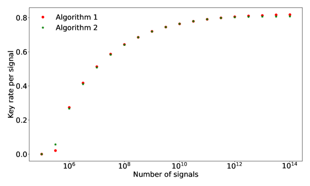
When applying Section 6.2 to the finite-key rate calculation, we optimize the min-tradeoff functions by choosing different $\bm{q}_{0}=(Q,1-Q)$ where $Q$ is searched over the interval $[0.005,0.07]$ with a step size $0.005$. For each min-tradeoff function generated from a particular value of $Q$, we calculate the key rate, which is the key length $\ell$ divided by the total number of signals $n$. We then choose the maximum key rate among all possible choices of min-tradeoff functions generated in this way. This way of coarse-grained search over $\bm{q}_{0}$ is a heuristic approach to optimize the choice of min-tradeoff functions. We find these choices of $\bm{q}_{0}$ in general give us good results. However, a more sophisticated optimization over $\bm{q}_{0}$ might potentially improve the results presented here.

For Section 6.3, we use the interior-point method from Matlab’s fmincon function for the first step and then use CVX for the linearized dual problem. We note that we can also use the Frank-Wolfe algorithm for the first step instead of the and the interior-point method. When we do so, results are similar (slightly worse) for this example.

For both algorithms, we optimize $p_{z}$ by optimizing $\gamma=(1-p_{z})^{2}=10^{-k}$ where $k$ is chosen from the interval $[2,4]$ with a step size of $0.1$. For block sizes larger than or equal to $10^{10}$, we allow $p_{z}$ to be closer to 1 by searching $k$ in the interval $[3,7]$ with a step size of $0.2$. Again, those choices are heuristic and could be potentially improved. Nevertheless, they are sufficient for our purpose.

Figure 3: Key rate versus the number of signals for the qubit BB84 protocol to compare different second-order correction terms using Section 6.3. The quantum bit error rate is set to $Q=0.01$ in the simulation. The red circle marker corresponds to the key rate formula given in Theorem 4 [26] while the green star marker corresponds to the key rate formula from Theorem 14 [16].

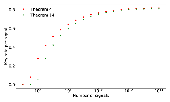
In Figure 2, we compare the key rates obtained from these two algorithms with Theorem 4. Interestingly, both algorithms give similar results while Section 6.3 seems to be slightly better in terms of the smallest number of signals for nonzero key rates. Intuitively, we expect Section 6.3 to behave better as it takes into account some second-order correction terms, while Section 6.2 only looks for the min-tradeoff function that gives the highest leading-order term. As we perform an optimization of the choice of min-tradeoff function by different initial $\bm{q}_{0}$’s for Section 6.2, we observe that the optimal finite key rate from Section 6.2 is often given by a min-tradeoff function that does not give the highest value for the leading-order term. Due to the optimization of $\bm{q}_{0}$, the running time of Section 6.2 is much longer than that of Section 6.3.

In Figure 3, we compare key rates given by Theorems 14 and 4 when we use Section 6.3. One can see that Theorem 4 gives better key rates. This confirms our conjecture that the EAT based on the sandwiched $\alpha$-Rényi entropy is tighter than the EAT based on the smooth min-entropy for lower-order correction terms. The intuition for this is that the Entropy Accumulation Theorem for smooth entropies is first derived in terms of $H_{\alpha}$ sandwiched Rényi entropies and then converted to statements about smooth entropies [15, 16]. It follows that avoiding the conversion to smooth entropies should only improve the key rate.

7.2 Six-state four-state protocol

Another interesting example is the six-state four-state protocol [27]. In the free space implementation of QKD protocols with the polarization encoding, there is naturally one axis that is stable against turbulence while other axes are slowly drifting. The idea of reference-frame-independent QKD [37] was motivated to address this issue and it was shown that such a protocol can be robust to slow drifts. The basic idea is that if the reference frame drift can be described by a unitary rotation, by using the information from an additional basis, one can effectively undo this unitary rotation. Here we consider the six-state four-state protocol [27] which has the reference-frame-independent feature. In particular, we consider the entanglement-based version and assume Alice and Bob have qubits. We do not consider losses in this example.

7.2.1 Protocol and simulation

We analyze the entanglement-based version of the six-state four-state protocol [27] assuming that Alice and Bob each receive a qubit in each round for simplicity of calculation. In this protocol, Alice measures the state in one of the $X,Y$ and $Z$ bases according to the probability distribution $((1-p_{z})/2,(1-p_{z})/2,p_{z})$, while Bob measures in one of $X$ and $Z$ bases with the probability distribution $(1-p_{z},p_{z})$. Similarly to the previous qubit BB84 example, when both Alice and Bob choose the $Z$ basis, this round is used for key generation. When Alice chooses $X$ or $Y$ basis and Bob chooses $X$ basis, this round is used for parameter estimation. All other rounds are discarded. We consider an efficient version by setting $p_{z}$ to be close to $1$. In the testing step of the protocol, we use the POVM that contains error rates in the $XX$ and $YX$ bases.

For the simulation, we assume the $Z$ basis is free of misalignment. The misalignment happens in the $X$-$Y$ plane of the Bloch sphere. Thus, on top of the qubit depolarizing channel, we also apply a unitary rotation along the $Z$ axis to Bob’s qubit in order to model the misalignment. We choose the angle of rotation to be $11^{\circ}$ in the simulation. The state used to obtain the observed statistics from this simulation is

$$\rho^{\text{sim}}=(\idm_{A}\otimes e^{i\theta\sigma_{Z}})\rho^{\text{dp}}(\idm_{A}\otimes e^{-i\theta\sigma_{Z}}),$$ (59)

where $\sigma_{Z}$ is the Pauli-$Z$ matrix, $\theta$ is the angle of rotation and $\rho^{\text{dp}}$ is the state given in Equation 58 (that is, the simulated state in the qubit-based BB84 example).

7.2.2 Results

In the application of Section 6.2 to the finite-key rate calculation, we optimize the min-tradeoff functions by choosing different $\bm{q}_{0}$’s. We adopt a heuristic approach to optimize the choice of min-tradeoff functions. Each $\bm{q}_{0}$ is created by choosing a different depolarizing probability $Q$, which is searched over the interval $[0.005,0.07]$ with a step size $0.005$. It is a heuristic choice that serves our purpose. For each min-tradeoff function generated from a particular value of $Q$, we calculate the key rate and then choose the maximum key rate among them. For Section 6.3, we use same procedure as for the qubit BB84 example in Section 7.1 including the optimization over the choice of $p_{z}$.

Figure 4: Key rate versus the number of signals for the six-state four-state protocol with two algorithms. The quantum bit error rate is set to $Q=0.01$ in the simulation. This plot is obtained by using the key rate formula given in Theorem 4 [26]. The red circle marker corresponds to the min-tradeoff function construction by Section 6.2 while the green star marker corresponds to the min-tradeoff function construction by Section 6.3.

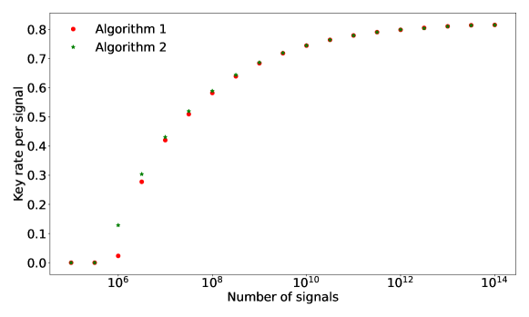
In Figure 4, we compare two algorithms for the min-tradeoff function construction. For this plot, similar to qubit-based BB84 example, we perform additional initial point $\bm{q}_{0}$ optimization for Section 6.2 while we do not optimize $\bm{q}_{0}$ for Section 6.3. Like Figure 2, both algorithms give similar key rates.

Figure 5: Key rate versus the number of signals for the six-state four-state protocol with different second-order correction terms. The quantum bit error rate is set to $Q=0.01$ in the simulation. This plot is obtained by using Section 6.3. The red circle marker corresponds to the key rate formula given in Theorem 4 [26] while the green star marker corresponds to the key rate formula from Theorem 14 [16].

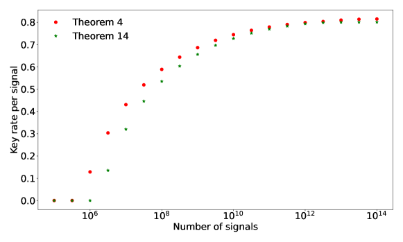
In Figure 5, we compare key rates for Theorems 14 and 4 and observe the same behavior as the qubit-based BB84 example in Figure 3. As explained in the qubit-based BB84 example in Figure 3, this behavior is not surprising since the sandwiched Rényi entropy was used in the middle step of the proofs of Theorems 10 and 1 in Refs. [15, 16] before converting to the smooth min-entropy by an additional inequality. One would expect that bypassing the smooth min-entropy gives tighter key rates due to the removal of an inequality.

7.3 High-dimensional 2-MUB protocol

To demonstrate an advantage of our approach in the EAT framework, we analyze an interesting family of protocols which are the high-dimensional analog of the BB84 protocol. In BB84, two mutually unbiased bases (MUBs) are used. We consider qudit systems with 2 MUBs. We compare our calculation with the postselection technique [14] combined with the numerical approach of [34]. We use this example to demonstrate that EAT can give better key rates compared to the postselection technique [14], especially when the dimension $\dim(\mathcal{H}_{AB})$ in the protocol is large.

7.3.1 Protocol and simulation

To properly define the protocol setup, recall that the discrete Weyl operators are defined as

$$U_{jk}=\sum_{s=0}^{d-1}\omega^{sk}\outerproduct{s+j}{s}$$ (60)

for $j,k\in\{0,1,\dots,d-1\}$ where $\omega=e^{2\pi i/d}$ is a $d$th root of unity. We note that $U_{01}$ is the generalized Pauli-$Z$ matrix and $U_{10}$ is the generalized Pauli-$X$ matrix. We define the qudit version of $Z$ and $X$ operators as $Z:=U_{01}$ and $X:=U_{10}$. The generalized Bell states are

$$\ket{\Phi_{jk}}=\frac{1}{\sqrt{d}}\sum_{s=0}^{d-1}\omega^{sk}\ket{s,s+j}=\idm\otimes U_{jk}\ket{\Phi_{00}}.$$ (61)

In the 2-MUB protocol, Alice measures in the eigenbasis of either $U_{01}$ or $U_{10}$. Bob similarly measures in the eigenbasis of either $U_{01}^{*}$ or $U_{10}^{*}$. The eigenbasis of the operator $Z:=U_{01}$ is the computational basis $\{\ket{s}:0\leq s\leq d-1\}$. The eigenbasis of the operator $X:=U_{10}$ is $\{\ket{\psi^{X}_{j}}:0\leq j\leq d-1\}$ where

$$\ket{\psi^{X}_{j}}:=\sum_{s=0}^{d-1}\frac{\omega^{-js}}{\sqrt{d}}\ket{s}.$$ (62)

They each choose to measure in the $Z$ basis with the probability $p_{z}$ and choose to measure in the $X$ basis with the probability $1-p_{z}$. In the classical phase, Alice and Bob announce their basis choices and discard rounds with mismatched bases. We allow an asymmetric basis choice, i.e., setting $p_{z}$ close to 1. In this protocol, all public announcements are based on seeded randomness. For simplicity of calculation, the testing rounds are those when they both choose $X$ basis and the key generation rounds are rounds when they both choose $Z$ basis.

It is interesting to note that the state $\ket{\Phi_{00}}=\frac{1}{\sqrt{d}}\sum_{s}\ket{s,s}$ is invariant under any $U_{jk}\otimes U^{*}_{jk}$. In an honest implementation, the source is supposed to prepare the state $\ket{\Phi_{00}}$, and then to distribute one half to Alice and the other half to Bob. If the quantum channel is ideal, then they are supposed to obtain perfectly correlated results just like the qubit case.

Following the reasoning of [38, 39], Alice’s and Bob’s joint density operator can be taken as diagonal in the generalized Bell basis:

$$\rho_{AB}^{\text{BG}}=\sum_{j,k}\lambda_{jk}\outerproduct{\Phi_{jk}}{\Phi_{jk}},$$ (63)

where

$$\lambda_{jk}=\frac{1}{d}\Big(\sum_{s}q_{1s}^{(sj-k\bmod d)}+q_{01}^{(j)}-1\Big)$$ (64)

with $q_{jk}^{(i)}$ being the $i$th entry of the error vector $\bm{q}_{jk}$. See also [40] for a detailed discussion. For our purpose of simulating the frequency distribution $\bm{q}_{0}$ needed for Section 6.2 or Section 6.3, we take the simulation state $\rho_{AB}^{\text{sim}}$ used to generate the full statistics as $\rho_{AB}^{\text{sim}}=\rho_{AB}^{\text{BG}}$.

We follow the simulation in [40] by considering the following observation for error vector $\bm{q}_{jk}$ in each basis $U_{jk}$, which is based on the natural generalization of the qubit depolarizing channel with a depolarizing probability $Q$:

$$\bm{q}_{jk}(Q):=\{1-Q,Q/(d-1),\dots,Q/(d-1)\}.$$ (65)

7.3.2 Results

(a)

(b)

Figure 6: 2-MUB protocols with qudits for various values of dimension $d$. The depolarizing probability is set to $Q=0.01$ in the simulation. The calculation is done with Section 6.3 and the finite-key rate formula is from Theorem 4 [26]. The calculation of postselection technique is done using the numerical approach of [34] in combination of [14]. The asymptotic key rate formula is given in [28, 40].

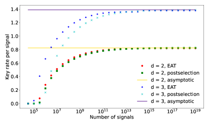
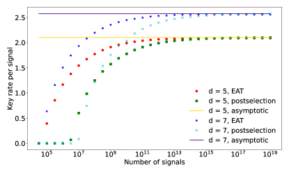
In Figure 6, we compare our results using Theorem 4 [26] with results obtained by the postselection technique [14] for 2-MUB protocols in dimensions $d=2,3,5$ and $7$. We note that 2-MUB protocols exist in any dimensions $d\geq 2$ and our proof method can work for any dimension. Here, we restrict to prime dimensions due to our choice of data simulation method. For both EAT and the postselection technique, we optimize the probability of choosing $Z$ basis. The probability of testing is set to $\gamma=(1-p_{z})^{2}$. We optimize the probability of choosing $Z$-basis in the same way as in the qubit-based BB84 example.

It can be seen that both EAT and postselection technique can approach the expected asymptotic key rate in the infinite-key limit. Also, our method based on EAT outperforms the postselection technique for 2-MUB protocols in any dimensions. We also observe that for larger dimensions, our method can give much higher key rate than the postselection technique for small block sizes. This makes our method attractive since small block sizes are of particular interests for experimental implementations.

In the same plot, we also show the asymptotic key rate for 2-MUB protocol. The asymptotic key rate formula is given in [28, 40]. Both our method and the postselection technique can approach the asymptotic key rate for sufficiently large block size. We also note that for block size larger than $10^{17}$, there seems to be a small constant deviation from the asymptotic key rate in both postselection technique and our method. This deviation is mainly due to our optimization over $p_{z}$, which is done by choosing a set of values. The asymptotic key rate formula that we use assumes that we can set $p_{z}$ to be arbitrarily close to $1$ such that the sifting factor is $1$. On the other hand, numerical optimization over $p_{z}$ in our method cannot take $p_{z}$ too close to one. The reason for our EAT method is that our testing probability is set to be $(1-p_{z})^{2}$. When the testing probability is small, the variance of the min-tradeoff function, $\mathsf{Var}(f)$, becomes large as shown in Equation 57. Since $\mathsf{Var}(f)$ shows up in the second-order correction term, for a fixed block size, there is always a limit on how small the testing probability $\gamma$ can be before we start to lose key rates due to its adverse effect on the second-order correction term. For a fair comparison between our EAT approach and the postselection technique, we also use the same optimization of $p_{z}$ in the calculation with the postselection technique.

7.4 BB84 with a realistic spontaneous parametric downconversion source

We consider an example where the Markov chain conditions are not simply based on seeded randomness. This example considers an optical implementation of entanglement-based BB84. The photon-pair source is a spontaneous parametric downconversion source where there is a non-negligible probability that the source emits vacuum or more than one photon pair. Due to photon loss during the transmission and non-unity detector efficiencies, there are no-detection events. In the protocol, Alice and Bob announce these events and discard the corresponding rounds. We need to verify that this type of announcements do not violate the Markov chain conditions.

7.4.1 Protocol and simulation method

In this protocol, a type-II parametric down-conversion (PDC) source emits a state with polarization encoding [41, 42] which is

$$\ket{\Psi}=(\cosh(\chi))^{-2}\sum_{n=0}^{\infty}\sqrt{n+1}\tanh^{n}(\chi)\ket{\Phi_{n}}$$ (66)

where $\ket{\Phi}_{n}$ is the state of an $n$-photon pair which can be written as

$$\ket{\Phi_{n}}=\frac{1}{\sqrt{n+1}}\sum_{m=0}^{n}(-1)^{m}\ket{n-m,m}_{a}\ket{m,n-m}_{b}.$$ (67)

The average number of photon pairs generated by one pump pulse is $2\lambda$, where $\lambda=\sinh(\chi)$. In this protocol, Alice and Bob each have a set of single-photon detectors. We consider the BB84 detector setup with a passive basis choice; that is, each measurement setup consists of an initial 50/50 beam splitter and each output port of this beam splitter is directed to a polarizing beam splitter with two single-photon detectors. We assume Alice’s two detectors have the same detector efficiency $\eta_{A}$ and the same dark count probability $Y_{0A}$. Similarly, we assume that Bob’s two detectors have the same detector efficiency $\eta_{B}$ and the same dark count probability $Y_{0B}$. Using the similar choice as in other examples, whenever Alice and Bob choose $X$-basis, the round is used for testing. The key generation round is when they both choose $Z$-basis. Their probabilities of choosing $Z$ basis is $p_{zA}$ and $p_{zB}$, respectively. The probability of testing is set to $\gamma=(1-p_{zA})(1-p_{zB})$.

Our simulation is based on [42]. In this simulation, there are three main contributions to quantum bit error rate: (i) background counts of detectors, which are random noises with $e_{0}=1/2$; (ii) intrinsic detector error $e_{d}$, which is the probability that a photon enters the erroneous detector and is used to characterized the alignment and stability of optical system between Alice’s and Bob’s detection systems; (iii) errors due to multiphoton-pair states: (a) Alice and Bob may detect different photon pairs and (b) double clicks from detectors. Alice and Bob assign a random bit for each double-click event in order to use the squashing model [43, 44].

In particular, the overall gain, $Q_{\lambda}$, as a function of the average number of photon, $\lambda$, in each mode, dark counts and detector efficiencies is given by [42, Eq. (9)]

$$Q_{\lambda}=1-\frac{1-Y_{0A}}{(1+\eta_{A}\lambda)}-\frac{1-Y_{0B}}{(1+\eta_{B}\lambda)}+\frac{(1-Y_{0A})(1-Y_{0B})}{(1+\eta_{A}\lambda+\eta_{B}\lambda-\eta_{A}\eta_{B}\lambda)^{2}}.$$ (68)

The overall quantum bit error rate ($E_{\lambda}$) is given by [42, Eq. (10)]

$$E_{\lambda}Q_{\lambda}=e_{0}Q_{\lambda}-\frac{2(e_{0}-e_{d})\eta_{A}\eta_{B}\lambda(1+\lambda)}{(1+\eta_{A}\lambda)(1+\eta_{B}\lambda)(1+\eta_{A}\lambda+\eta_{B}\lambda-\eta_{A}\eta_{B}\lambda)}.$$ (69)

To reduce the number of free parameters in the protocol setup, we set $p_{zA}=p_{zB}=p_{z}$ and the testing probability is set to $\gamma=(1-p_{z})^{2}$. We optimize the choice of $p_{z}$ in the same way as in Section 7.1.

7.4.2 Assumption on announcements

We need to verify for Markov chain conditions that the probability of a detection event only depends on the total photon number, but not on the particular $n$-photon state. We show that this holds when Alice’s (Bob’s) detectors consist of two single-photon detectors with an identical detection efficiency $\eta_{A}$ ($\eta_{B}$), and a basis-independent dark count probability $Y_{0A}$ ($Y_{0B}$). We note that the measurement performed by Bob (Alice) is block diagonal in the total photon number basis, as is the case in all discrete-variable protocols.

Under our assumption about the detectors, we can treat all the imperfections of detectors as a part of the quantum channel and then assume ideal detectors in our analysis. Doing so only strengthens Eve’s power. After assigning double-click events to random bits, we note that the measurement setup in this protocol admits a squashing model [43, 44]. In our analysis, we can use the effective qubit measurement for Alice (Bob) as the target measurement. This target measurement acts on the Hilbert space that consists of a one-dimensional vacuum space and a two-dimensional qubit space. In particular, the announcement about detection and no-detection corresponds to the POVM $\{M_{\text{det}},M_{\text{no-det}}\}$, which is defined as

$$M_{\text{det}}=\begin{pmatrix}0&0&0\\ 0&1&0\\ 0&0&1\end{pmatrix},\,M_{\text{no-det}}=\begin{pmatrix}1&0&0\\ 0&0&0\\ 0&0&0\end{pmatrix},$$ (70)

where they are represented in the basis $\{\ket{\text{vac}},\ket{0},\ket{1}\}$. Here $\ket{\text{vac}}$ is the vacuum state and $\ket{0},\ket{1}$ are the computational basis states of a qubit. Clearly, this POVM is weekly dependent according to Definition 3. Thus, this announcement is allowed in applying Theorem 4.

7.4.3 Results

Figure 7: Key rate per signal sent versus the number of signals for BB84 with a spontaneous parametric downconversion source for various distances between Alice and Bob. This plot is obtained with Section 6.2 and Theorem 4. Parameters are specified in the main text.

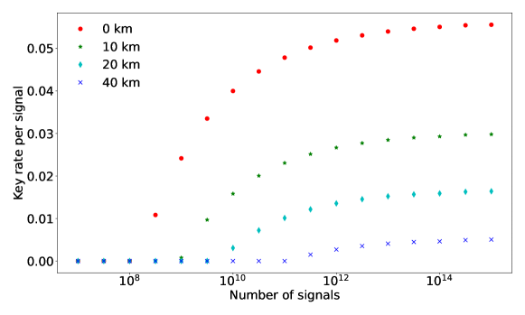
In Figure 7, we show the key rate of this protocol for different distances ($L$ in kilometers) between Alice and Bob. We assume the source is located in the middle and at an equal distance from Alice and Bob. We choose detector efficiencies $\eta_{A}=\eta_{B}=0.8$ and dark counts $Y_{0A}=Y_{0B}=10^{-7}$ for the simulation in this plot. We also set the intrinsic detector error $e_{d}$ as $1\%$. On one hand, we can see that our method works for optical implementations from this figure. On the other hand, as the distance between Alice and Bob increases, the minimal number of signals for positive key rate also increases significantly and the key rate drops quickly. In our key rate expression from Theorem 4 (also from Theorem 14), the term $-n\gamma\log(\abs{\cA})$ decreases the key length and becomes more problematic for this protocol since the entropy only accumulates in rounds where both Alice and Bob successfully detected photons. However, this term does not scale with the probability of detection. For long distances, this seems to suggest that the cost for parameter estimation is higher than the entropy accumulated from rounds with successful detection. Unfortunately, this counter-intuitive effect comes from the limitation of our proof method in dealing with parameter estimation registers. We hope that a better approach to handle the information leakage from parameter estimation step can be found in the future to significantly improve the key rate.

8 Discussion and Conclusion

In this work, we have adapted the EAT to entanglement-based device-dependent QKD protocols. To do so, we introduced new tools. First, we constructed new sufficient conditions on the public announcements of the protocol to guarantee the Markov conditions necessary for the EAT. These conditions capture the intuition that if Eve would always know some information for each round of the protocol, then announcing that information cannot change the security. The interesting point is that this guarantees the Markov conditions on Eve’s optimal attack.

Second, we proposed two variants of a numerical algorithm to construct min-tradeoff functions, both of which are efficient and one which considers second-order effects. Both methods build off of previous work [24, 25], but the ability to construct min-tradeoff functions that take into account second-order correction information is novel and we expect could be useful in other settings. We note this second-order correction algorithm relies on using Fenchel duality, which to the best of our knowledge has not been used in quantum information theory previously.

Third, we derived our key length bound (Theorem 4) using Dupuis’ privacy amplification for sandwiched Rényi entropies $H^{\uparrow}_{\alpha}$ [26]. In that work, Dupuis demonstrates one can obtain simpler error exponents for privacy amplification using the Rényi version of the EAT along with his Rényi leftover hashing lemma [26, Theorem 9] than if one were to apply the smooth min-entropy leftover hashing lemma [13]. Here we have shown an alternative advantage: by avoiding the conversion of the Rényi EAT into smooth min-entropy terms, we can tighten our bound on the key rate.

We then apply our methods to several examples. First, we applied it to ideal qubit-based BB84 and six-state four-state protocols where we show the application of both our min-tradeoff construction algorithms and that using our Rényi entropy rate improves the finite-size key rate to considering the smooth min-entropy rate, at least in the current proof method. We next considered the high-dimensional two mutually unbiased bases protocols which exemplified an improvement in the key rate over the postselection technique [14], an alternative proof method for coherent-attack security which is limited in how it scales with respect to the dimension of Alice and Bob’s quantum states. This confirms there is a regime in which the postselection technique is “loose”, further suggesting the importance of the application of the EAT. Lastly, we demonstrate our method for an optical implementation. This example demonstrates that our method is also applicable to practical protocols instead of restricting to theoretically simple ones. On the other hand, due to unsatisfactory results in small block sizes, we also observe that the EAT currently appears to require more improvements in handling loss and noise in order to have good key rates for experimentally feasible block sizes.

Given these results, it is natural to consider where improvements might be made or further avenues to explore. First and foremost, we note that we were restricted to considering entanglement-based protocols as we need the entanglement-based protocol framework to use our algorithms. In previous work [34], this has not been limiting as we could use the source-replacement scheme [45, 28] to convert prepare-and-measure protocols to entanglement-based ones. However, it is not clear how the source-replacement scheme interacts with the Markov chain requirements for the EAT, which is why this work is restricted to entanglement-based protocols. Second, we have seen that while the EAT scales well in terms of the dimension of the states, it seems limited by loss and noise. In particular, the ability to handling high loss parameter regime is of particular interest for realistic implementations. As such, a natural question is to try and find ways to make the EAT more robust to loss and noise, at least in the device-dependent setting.

Appendix A A Sufficient Condition for the Markov Chain Condition

In this section, we prove Theorem 2 from the main text which gives sufficient conditions for ensuring the Markov chain conditions hold on the optimal attack. We note the statement in this section (5) includes an additional equivalent condition which is quick to verify and so may be of use.

Recall that we consider EAT channels with a special tensor product structure. We consider $n$ CPTP maps $\widetilde{\mathcal{M}}_{i}:Q_{i}\rightarrow S_{i}P_{i}X_{i}$ acting in tensor product on the $n$ independent systems $\{Q_{i}\}_{i}$. The maps are defined by the POVM $\{M_{sp}\}$ such that

$$\widetilde{\mathcal{M}}_{i}(\rho)=\sum_{s,p}\Tr[\rho M_{sp}]\outerproduct{s,p}{s,p}_{S_{i}P_{i}}\otimes\outerproduct{t(s,p)}{t(s,p)}_{X_{i}}\,.$$ (71)

From these we define the corresponding EAT channels $\mathcal{M}_{i}:R_{i-1}\rightarrow R_{i}S_{i}P_{i}X_{i}$ acting on the quantum systems $R_{i}=Q_{i+1}^{n}$, as $\mathcal{M}_{i}=\widetilde{\mathcal{M}}_{i}\otimes\id_{Q_{i+1}^{n}}$ (see main text for further details). In this case, it is simple to prove that the output state of the protocol $\rho_{S_{1}^{n}P_{1}^{n}X_{1}^{n}E}=\mathcal{M}_{1}\circ\dots\circ\mathcal{M}_{n}\otimes\id_{E}(\rho_{R_{0}E})$ takes on the simple form

$$\rho_{S_{1}^{n}P_{1}^{n}X_{1}^{n}E}=\bigotimes_{i=1}^{n}\widetilde{\mathcal{M}}_{i}\otimes\id_{E}(\rho_{Q_{1}^{n}E})$$ (72)

where $R_{0}=Q_{1}^{n}$.

We now want to prove the following proposition.

Proposition 5.

Let $\{M_{sp}:s\in\mathcal{S},p\in\mathcal{P}\}$ be the POVM associated to a given quantum-to-classical CPTP map $\widetilde{\mathcal{M}}_{i}:Q_{i}\rightarrow S_{i}P_{i}X_{i}$ and let $M_{p}:=\sum_{s}M_{sp}$ correspond to the POVM elements of the map $\Tr_{S_{i}X_{i}}\circ\widetilde{\mathcal{M}}_{i}:Q_{i}\rightarrow P_{i}$. If either item (A) or item (B) below holds for each CPTP map $\widetilde{\mathcal{M}}_{i}$, then without loss of generality the optimal attack by an eavesdropper is of a block-diagonal form such that the Markov chain conditions, Equation 8, hold and so the EAT may be applied (Theorem 1).

1. There exists a decomposition $Q_{i}=\bigoplus_{\lambda}V^{\lambda}$ of the space $Q_{i}$ into orthogonal subspaces $\{V^{\lambda}\}_{\lambda}$ such that

   • For all $(s,p)\in\mathcal{S}\times\mathcal{P}$, $M_{sp}$ is block diagonal: $M_{sp}=\bigoplus_{\lambda}M^{(\lambda)}_{sp}$, where $M_{sp}^{(\lambda)}$ acts on the subspace $V^{\lambda}$.

   • For all $p\in\mathcal{P}$, $M_{p}$ is block diagonal and proportional to the identity in each subspace: there exist constants $m_{p}^{\lambda}\in[0,1]$ such that $M_{p}=\bigoplus_{\lambda}m_{p}^{\lambda}\idm_{V^{\lambda}}$, where $\idm_{V^{\lambda}}$ is the identity operator on $V^{\lambda}$.

2. For all $s\in\mathcal{S}$, $p,p^{\prime}\in\mathcal{P}$, $M_{sp}$ and $M_{p^{\prime}}$ commute: $[M_{sp},M_{p^{\prime}}]=0$.

Furthermore, (A) and (B) are equivalent.

Remark 12.

The statement of Theorem 2 just states item (A) in 5 under the name of ‘weakly dependent’ (Definition 3), which is of primary interest. While equivalent, item (B) is stated here as it could be of use when one knows the measurement operators, as it is then easy to check item (B) to determine if 5 may be applied.

One way to prove the EAT theorem applies under item (A) or item (B) would be to show the output state in Equation 72 satisfies the Markov chain conditions, but this does not work in general. Instead, we show that we can assume the initial state is of a certain block diagonal form without loss of generality due to the block diagonal structure of the EAT channels (Lemma 1). Then we show that this block diagonal form satisfies the Markov chain conditions (Proof of 5), and, as assuming this form was without loss of generality, this is sufficient. The reduction to a quantum state with block-diagonal structure is well-known in discrete-variable QKD where the measurement operators that model single-photon detectors are block diagonal in the total photon number basis. In such a setting, this block diagonal structure implies Eve’s optimal attack includes implementing a QND measurement on the total number of photons before sending out the states, thereby resulting in the state being block-diagonal without loss of generality. One may view Lemma 1 and 5 as a generalization of such a method, but with the further insight that such structure implies the Markov chain conditions hold.

Lemma 1.

Let each $\widetilde{\mathcal{M}}_{i}$ be a quantum-to-classical CPTP map whose associated POVM elements are block diagonal; i.e., for each $i$ there exists a decomposition $Q_{i}=\bigoplus_{\lambda}V^{\lambda}$ such that $M_{sp}=\bigoplus_{\lambda}M_{sp}^{(\lambda)}$ with $M_{sp}^{(\lambda)}$ acting on $V^{\lambda}$. Then for any initial state $\rho_{Q_{1}^{n}E}$, there exists another state $\nu_{Q_{1}^{n}E^{\prime}}$ such that

• the state $\nu_{Q_{1}^{n}E^{\prime}}$ has the block diagonal form

  $$\nu_{Q_{1}^{n}E\Lambda_{1}^{n}}=\sum_{\bm{\lambda}=(\lambda_{1},\cdots\lambda_{n})}\rho_{Q_{1}^{n}E}{(\bm{\lambda})}\otimes\outerproduct{ \vect{\lambda}}{ \vect{\lambda}}_{\Lambda_{1}^{n}}\,,$$ (73)

  where Eve’s registers $E^{\prime}=(E,\Lambda_{1},\cdots\Lambda_{n})$ are composed of a quantum memory $E$ and $n$ classical registers $\Lambda_{i}$ indicating the subspace, so that, for all $\bm{\lambda}$, the state $\Tr_{E}[\rho_{Q_{1}^{n}E}{(\bm{\lambda})}]$ is defined on $V^{\bm{\lambda}}:=\bigotimes_{i}V^{\lambda_{i}}$, and

• the output states $\nu_{S_{1}^{n}P_{1}^{n}X_{1}^{n}E^{\prime}}$ and $\rho_{S_{1}^{n}P_{1}^{n}X_{1}^{n}E}$ are related by

  $$\Tr_{\Lambda_{1}^{n}}[\nu_{S_{1}^{n}P_{1}^{n}X_{1}^{n}E\Lambda_{1}^{n}}]=\rho_{S_{1}^{n}P_{1}^{n}X_{1}^{n}E}\,.$$ (74)

Proof.

To construct the state $\nu_{Q_{1}^{n}E^{\prime}}$ from the state $\rho_{Q_{1}^{n}E}$, we consider the dephasing map $\Delta_{i}:Q_{i}\rightarrow Q_{i}\Lambda_{i}$

$$\Delta_{i}(\rho)={\sum}_{\lambda}P_{\lambda}\rho P_{\lambda}\otimes\outerproduct{\lambda}{\lambda}_{\Lambda_{i}}\,,$$ (75)

where $P_{\lambda}$ is a projector on the subspace $V^{\lambda}$. This map $\Delta_{i}$ projects the state onto each subspace $V^{\lambda}$ without affecting the coherence inside the subspace $V^{\lambda}$ and writes the result in $\Lambda_{i}$. We then define $\nu_{Q_{1}^{n}E^{\prime}}:=\nu_{Q_{1}^{n}E\Lambda_{1}^{n}}:=\left(\bigotimes_{i}\Delta_{i}\otimes\id_{E}\right)(\rho_{Q_{1}^{n}E})$. The state $\nu_{Q_{1}^{n}E\Lambda_{1}^{n}}$ is indeed of the form Equation 73, as required.

Because of the block diagonal structure of the maps $\widetilde{\mathcal{M}}_{i}$, it is simple to see that the dephasing map does not affect the measurement statistics. We can observe that the maps $\Delta_{i}$ and $\widetilde{\mathcal{M}}_{i}$ are related by $\Tr_{\Lambda_{i}}\circ\widetilde{\mathcal{M}}_{i}\circ\Delta_{i}=\widetilde{\mathcal{M}}_{i}\circ\Tr_{\Lambda_{i}}\circ\Delta_{i}=\widetilde{\mathcal{M}}_{i}$. Consequently, we have

$$\Tr_{\Lambda_{1}^{n}}[\nu_{S_{1}^{n}P_{1}^{n}X_{1}^{n}E\Lambda_{1}^{n}}] =\Tr_{\Lambda_{1}^{n}}\circ\left(\bigotimes_{i}\widetilde{\mathcal{M}}_{i}\otimes\id_{E\Lambda_{1}^{n}}\right)\circ\left(\bigotimes_{i}\Delta_{i}\otimes\id_{E}\right)(\rho_{Q_{1}^{n}E})$$ (76)

$$=\left(\bigotimes_{i}\widetilde{\mathcal{M}}_{i}\otimes\id_{E}\right)(\rho_{Q_{1}^{n}E})$$ (77)

$$=:\rho_{S_{1}^{n}P_{1}^{n}X_{1}^{n}E}.$$ (78)

∎

Proof of 5.

Let $\rho_{Q_{1}^{n}E}$ be some initial state used in the EAT (Theorem 1). We assume that the maps $\widetilde{\mathcal{M}}_{i}$ satisfy the item (A) instead of the Markov chain conditions. Let us show that the Markov chain conditions follow from this condition.

Using the block diagonal structure of item (A), we can use Lemma 1 to show that there exists a block diagonal state $\nu_{Q_{1}^{n}E^{\prime}}$ with the same passing probability $\nu[\Omega]=\rho[\Omega]$, which satisfies $H_{\min}^{\epsilon}(S_{i}^{n}|P_{i}^{n}E)_{\rho_{|\Omega}}\geq H_{\min}^{\epsilon}(S_{i}^{n}|P_{i}^{n}E^{\prime})_{\nu_{|\Omega}}$. Indeed, this follows by using Equation 74 and the strong subadditivity of smooth min-entropies. We conclude that whatever min-entropy lower-bound statement holds for $\nu_{Q_{1}^{n}E^{\prime}}$ must also hold for $\rho_{Q_{1}^{n}E}$.

To prove 5, we then show that the new state $\nu_{Q_{1}^{n}E}$ satisfies the Markov chain conditions in Equation 8. We can do this by showing that given the state $\nu_{S_{1}^{i-1}P_{1}^{i-1}E^{\prime}}$, there exists a recovery map $\mathcal{R}_{P_{i}E\leftarrow E^{\prime}}$ which acts on Eve’s registers $E^{\prime}=(E,\Lambda_{1}^{n})$ and recovers the register $P_{i}$, i.e., $\mathcal{R}(\nu_{S_{1}^{i-1}P_{1}^{i-1}E^{\prime}})=\nu_{S_{1}^{i-1}P_{1}^{i}E}$. Since the POVM elements $M_{p}$ are proportional to the identity in every subspace $V^{\lambda}$, the probability distribution of $P_{i}$ only depends on the subspace $V^{\lambda}$, which is indicated in Eve’s register $\Lambda_{i}$. This means the variable $P_{i}$ can therefore be recovered from $\Lambda_{i}$ by simply generating it with the distribution $\Pr_{P}(p|\lambda)=m_{p}^{\lambda}$. Moreover, as we have shown the Markov chain conditions for $\nu_{Q^{n}_{1}E^{\prime}}$ and without loss of generality, Eve can only do better using a state of the form $\nu$, we can conclude we may use the EAT (Theorem 1) to prove security.

Having shown that the Markov chain conditions follow from item (A), it remains to show that (A) and (B) are equivalent. To do so, we first note that the commutation relation $[M_{sp},M_{p^{\prime}}]=0$ in item (B) is a direct consequence of the block diagonal conditions in (A). Conversely, we note that by construction the POVM elements $M_{p}$’s are linear combinations of the measurement operators $M_{sp}$’s. Therefore, the commutation relation in item (B) implies the commutation relation $[M_{p},M_{p^{\prime}}]=0$ for all $p,p^{\prime}\in\mathcal{P}$. This consequently implies the existence of a joint basis that simultaneously diagonalizes the operators $M_{p}$’s. We can thus find an orthogonal decomposition $V^{\lambda}$ so that $M_{p}=\bigoplus_{\lambda}m_{p}^{\lambda}\idm_{V^{\lambda}}$. Using the commutation relation in item (B) a second time implies that the operators $M_{sp}$ must be block diagonal along the same subspaces $V^{\lambda}$’s. ∎

Remark 13.

We note this proof does not change for Rényi entropies as they also satisfy strong subadditivity.

Appendix B Security of QKD using EAT without Smoothing

In this appendix, we present the necessary technical lemmas and the resulting proof for Theorem 4. The primary tool is Dupuis’ recent result on applying privacy amplification without smoothing [26]. However, we will also need to prove a max-tradeoff function upper bound on $H^{\uparrow}_{\alpha}(S_{1}^{n}|P_{1}^{n}E)_{\rho_{|\Omega}}$. We note that in the original work [15] a max-tradeoff function upper bound for $H^{\uparrow}_{\alpha}$ is implied to be straightforward given the max-tradeoff result presented in said work and simply not presented because upper bounding an alternative entropy will result in a tighter bound on $H^{\varepsilon}_{\max}$ [15, Footnote 13]. For completeness, we present our proof of such a bound. Throughout this appendix we present results using the Greek letters $(\alpha,\beta,...)$ that will be ultimately used in our key length security result rather than always using $\alpha$ for the Rényi entropy, so that it is easier to see how the results combine. We refer to Section 2.1 for a summary of common notations. We do however use $A_{i}$ and $B_{i}$ rather than $S_{i}$ and $P_{i}$ respectively from the main text.

B.1 Background Rényi divergence results

Here we present the special cases of the Rényi entropy chain rules which we will need in this section. We refer to Section 2.1 for basic entropic notation used in this work.

Theorem 6 ([46, Theorem 1]).

Let $\rho_{ABC}\in\mathrm{D}(ABC)$, $\tau_{C}\in\mathrm{D}(C)$, $\alpha,\beta,\gamma\in(1/2,1)\cup(1,\infty)$ such that $\frac{\alpha}{\alpha-1}=\frac{\beta}{\beta-1}+\frac{\gamma}{\gamma-1}$.

1. Case 1: If $(\alpha-1)(\beta-1)(\gamma-1)>0$,  $H_{\beta}^{\uparrow}(A|BC)_{\rho}\leq H_{\alpha}(\rho_{ABC}||\tau_{C})-H_{\gamma}(\rho_{BC}||\tau_{C})\ .$

2. Case 2: If $(\alpha-1)(\beta-1)(\gamma-1)<0$,  $H_{\alpha}(\rho_{ABC}||\tau_{C})\leq H^{\uparrow}_{\beta}(A|BC)_{\rho}+H_{\gamma}(\rho_{BC}||\tau_{C})\ .$

Remark 14.

In Ref. [46], the result is presented with the product $(\alpha-1)(\beta-1)(\gamma-1)$ to be bounded by one rather than zero. If one checks the conditions used to derive the theorem ([46, Propositions 7 and 8]), it only depends on the sign of the product. This has been realized in previous works, e.g. [29].

Corollary 7 (Special Cases of Chain Rules).

Let $\rho_{ABC}\in\mathrm{D}(ABC)$, $\tau_{C}\in\mathrm{D}(C)$. Let $\alpha,\beta,\delta,\eta,\gamma,\zeta\in(1/2,1)\cup(1,\infty)$.

1. Let $(\eta-1)(\delta-1)(\zeta-1)>0$, $\frac{\eta}{\eta-1}=\frac{\delta}{\delta-1}+\frac{\zeta}{\zeta-1}$ and $B$ be a trivial (one-dimensional) register. Then $H_{\delta}^{\uparrow}(A|C)_{\rho}\leq H_{\eta}(\rho_{AC}||\tau_{C})+D_{\zeta}(\rho_{C}||\tau_{C})\ .$

2. Let $(\alpha-1)(\beta-1)(\delta-1)<0$ and $\frac{\beta}{\beta-1}=\frac{\alpha}{\alpha-1}+\frac{\delta}{\delta-1}$. Then $H^{\uparrow}_{\beta}(AB|C)_{\rho}\leq H^{\uparrow}_{\alpha}(A|BC)_{\rho}+H^{\uparrow}_{\delta}(B|C)_{\rho}\ .$

Proof.

Item 1 follows from Item 1 of Theorem 6 by noting if $B$ is trivial, the $B$ register may be dropped. Because $H_{\gamma}(\rho_{BC}||\tau_{C})=-D_{\gamma}(\rho_{C}||\idm_{\mathbb{C}}\otimes\tau_{C})$, the negative signs cancel. Dropping the register $B$ and setting $\beta\to\delta$, $\alpha\to\eta$, and $\gamma\to\zeta$ completes the proof. Item 2 follows from Item 2 of Theorem 6 by letting $\tau_{C}$ be the optimizer for $H^{\uparrow}_{\alpha}(AB|C)_{\rho}$. Then by definition, $H^{\uparrow}_{\gamma}(B|C)_{\rho}\geq H_{\gamma}(\rho_{BC}||\tau_{C})$. Relabeling by $\alpha\to\beta$, $\beta\to\alpha$, $\gamma\to\delta$ completes the proof. ∎

B.2 Applying privacy amplification without smoothing

In Ref. [26], it was shown that privacy amplification could be performed without smoothing. While it was stated as holding for strongly 2-universal hashing functions, it is straightforward to show that the proof is the same for a general family of 2-universal hash functions. Recall that a family of 2-universal hash functions is the pair $(p_{F},\mathcal{F})$ where $\mathcal{F}$ is a set of functions from discrete alphabet $\mathcal{X}$ to discrete alphabet $\mathcal{Z}$ and $p_{f}$ is a probability distribution over $\mathcal{F}$ such that $\Pr_{f}[f(x)=f(x^{\prime})]\leq|\mathcal{Z}|^{-1}$ for all $x\neq x^{\prime}\in\mathcal{X}$. Altering notation to better fit for our purposes, Theorem 8 of Ref. [26] is in terms of $\mathbb{E}_{f\in\mathcal{F}}\left\|\rho_{ZE}^{f}-\frac{1}{|\{0,1\}^{\ell}|}\mathbb{1}_{Z}\otimes\rho_{E}\right\|_{1}$ where $\rho^{f}_{ZE}$ is $\rho_{XE}$ after the hash function $f$ has been applied to register $X$ and $\mathcal{Z}=\{0,1\}^{\ell}$. Using that announcing the choice of hash function $f\in\mathcal{F}$ will make the state block diagonal in the register $F$ that stores this announcement, it is clear that

$$\|\rho_{ZEF}-\frac{1}{|\{0,1\}^{\ell}|}\mathbb{1}_{Z}\otimes\rho_{EF}\|_{1} =\sum_{f}p(f)\|\rho^{f}_{ZE}-\frac{1}{|\{0,1\}^{\ell}|}\mathbb{1}_{Z}\otimes\rho_{E}\|_{1}$$

$$=\mathbb{E}_{f}\|\rho^{f}_{ZE}-\frac{1}{|\{0,1\}^{\ell}|}\mathbb{1}_{Z}\otimes\rho_{E}\|_{1}\ ,$$

so we state the result in the fashion more commonly used in QKD.

Proposition 6 (Special Case of [26, Theorem 8]).

Let $\rho_{XE}\in\mathrm{D}(XE)$ be a classical-quantum state where $X\cong\mathbb{C}^{|\mathcal{X}|}$ where $\mathcal{X}$ is some finite set. Let $(p_{f},\mathcal{F})$ be a family of two-universal hash functions from $\mathcal{X}\to\mathcal{Z}$ and $\mathcal{Z}=\{0,1\}^{\ell}$. Let $\alpha\in(1,2)$. Then

$$\left\|\rho_{ZEF}-\frac{1}{|\{0,1\}^{\ell}|}\mathbb{1}_{Z}\otimes\rho_{EF}\right\|_{1}\leq 2^{\frac{2}{\alpha}-1}\cdot 2^{\frac{1-\alpha}{\alpha}\left(H_{\alpha}^{\uparrow}(X|E)_{\rho}-\ell\right)}\ ,$$

where $F$ is the register storing the announcement of the hash function.

From this we obtain the following corollary immediately.

Corollary 8.

Let $\rho_{XE{|\Omega}}\in\mathrm{D}(XE)$ be a classical-quantum state. Let $\varepsilon_{sec}:=\frac{1}{2}\cdot 2^{\frac{2}{\alpha}-1}\cdot 2^{\frac{1-\alpha}{\alpha}\left(H_{\alpha}^{\uparrow}(X|E)_{\rho}-\ell\right)}$ where $\alpha\in(1,2)$. Then for an $\varepsilon_{sec}$-secret key, the length of the key, $\ell$, must satisfy the following bound:

$$\ell\leq H^{\uparrow}_{\alpha}(X|E)_{\rho}-\frac{\alpha}{\alpha-1}\log(\frac{1}{\vSec})+2\ .$$

Proof.

Starting from how we defined $\varepsilon_{\text{\rm sec}}$:

$$\varepsilon_{\text{\rm sec}}\leq 2^{\frac{2}{\alpha}-2}\cdot 2^{\frac{1-\alpha}{\alpha}\left(H_{\alpha}^{\uparrow}(X|E)_{\rho}-\ell\right)}$$

$$\Rightarrow \log(\vSec)\leq\frac{2}{\alpha}-2+\frac{1-\alpha}{\alpha}\left(H_{\alpha}^{\uparrow}(X|E)_{\rho}-\ell\right)$$

$$\Rightarrow \frac{1-\alpha}{\alpha}\ell\leq\frac{2}{\alpha}-2+\frac{1-\alpha}{\alpha}H_{\alpha}^{\uparrow}(X|E)_{\rho}+\log(\frac{1}{\vSec})$$

$$\Rightarrow \ell\leq H^{\uparrow}_{\alpha}(X|E)_{\rho}+\frac{\alpha}{1-\alpha}\log(\frac{1}{\vSec})+2\ .$$

Pulling a negative sign out of the $\frac{\alpha}{1-\alpha}$ term completes the proof. ∎

Remark 15.

Note we added the $\frac{1}{2}$ term in defining $\varepsilon_{\text{\rm sec}}$ because trace distance should be divided by two for the operational interpretation.

B.3 Entropy Accumulation Theorem for upper bound on $H_{\delta}^{\uparrow}$

In this section we prove an upper bound on $H^{\uparrow}_{\delta}$ in terms of a max-tradeoff function. While almost all of the work is done by [15], we split it into two pieces as we will need to use a chain rule and also as it allows us to specify what results of [15] we use at each step. As explained earlier, this result is implied to be expected to exist in some form in [15, Footnote 13]. We present it in its entirety for rigour.

As we switched the secret and public register notation, we emphasize in the current notation the Markov conditions are:

$$A_{1}^{i-1}\leftrightarrow B_{1}^{i-1}E\leftrightarrow B_{i}\qquad\forall i\in\{1,\ldots,n\}\ .$$ (79)

We proceed by using the original entropy price function which we know is sub-optimal in the second-order terms, but that will not matter for our purposes. For every $i$, we use a CPTP map $\mathcal{D}_{i}:X_{i}\to X_{i}D_{i}\overline{D}_{i}$

$$\mathcal{D}_{i}(W_{X_{i}})=\sum_{x\in\mathcal{X}}\bra{x}W_{X_{i}}\ket{x}\outerproduct{x}{x}\otimes\tau(x)_{D_{i}\overline{D}_{i}}\ ,$$

where $\tau(x)_{D_{i}\overline{D}_{i}}$ is such that $H(D_{i}|\overline{D}_{i})_{\tau(x)}=\overline{g}-f(\delta_{x})$, $f$ is a min-tradeoff function, $[g_{\min},g_{\max}]$ is the smallest real interval containing $f({{\mathbb{P}}}(\mathcal{X}))$ and $\overline{g}:=(g_{\min}+g_{\max})/2$. This is possible by letting $\tau(x)_{D_{i}\overline{D}_{i}}$ be a mixture of the maximally entangled state and the maximally mixed state. Following the argument from [15, Beginning of Proof of Proposition 4.5], this can be done if $|D_{i}|\leq\exp(\lceil\|\nabla f\|_{\infty} \rceil)$. We also note the general definition $\overline{\rho}:=(\mathcal{D}_{n}\circ\ldots\circ\mathcal{D}_{1})(\rho)$. With all of this specified, we begin with our equivalent of Claim 4.6 of [15].

Lemma 2.

Let $\delta\in[1/2,\infty)$. Assuming the Markov chain conditions are satisfied [Equation 79], then

$$H^{\uparrow}_{\delta}(A^{n}_{1}|B^{n}_{1}E)_{\rho_{|\Omega}}\leq H^{\uparrow}_{\delta}(A^{n}_{1}D^{n}_{1}|B^{n}_{1}E\overline{D}^{n}_{1})_{\overline{\rho}_{|\Omega}}+nh-n\overline{g}\ ,$$

where $h\in\mathbb{R}$ that satisfies the conditions assumed in Theorem 1 and $\overline{g}$ is as defined above.

Proof.

First note that

$$\overline{\rho}_{A^{n}_{1}X^{n}_{1}B^{n}_{1}E\overline{D}^{n}_{1}|\Omega}=\frac{1}{\rho[\Omega]}\sum_{x^{n}_{1}\in\Omega}\outerproduct{x^{n}_{1}}{x^{n}_{1}}\otimes\rho_{A^{n}_{1}B^{n}_{1}E,x^{n}_{1}}\otimes\Tr_{D^{n}_{1}}(\tau(x^{n}_{1})_{D^{n}_{1}\overline{D}^{n}_{1}})\ .$$

Note that $\Tr_{D_{i}}(\tau(x_{i})_{D_{i}\overline{D}_{i}})=\frac{1}{\absolutevalue{\ol{D}_{i}}}\idm_{\overline{D}_{i}}$ for all $i$ and $x_{i}$ because $\tau(x_{i})$ is a mixture of the maximally mixed and maximally entangled state. It follows we know that register is independent of the rest of the registers and that

$$\overline{\rho}_{A^{n}_{1}X^{n}_{1}B^{n}_{1}E\overline{D}^{n}_{1}|\Omega}=\frac{1}{\rho[\Omega]}\sum_{x^{n}_{1}\in\Omega}\outerproduct{x^{n}_{1}}{x^{n}_{1}}\otimes\rho_{A^{n}_{1}B^{n}_{1}E,x^{n}_{1}}\otimes\overline{\rho}_{\overline{D}^{n}_{1}}\ .$$ (80)

It follows the state is invariant under tracing off $\overline{\rho}_{\overline{D}^{n}_{1}}$ and re-appending it. Denote this map $\mathcal{R}$. By data-processing,

$$-D_{\delta}(\rho_{A^{n}_{1}X^{n}_{1}B^{n}_{1}E\overline{D}^{n}_{1}}||\idm_{A^{n}_{1}X^{n}_{1}}\otimes\sigma_{B^{n}_{1}E\overline{D}^{n}_{1}})_{\overline{\rho}_{|\Omega}}\,\leq \,-D_{\delta}(\mathcal{R}(\rho_{A^{n}_{1}X^{n}_{1}B^{n}_{1}E\overline{D}^{n}_{1}})||\mathcal{R}(\idm_{A^{n}_{1}X^{n}_{1}}\otimes\sigma_{B^{n}_{1}E\overline{D}^{n}_{1}}))_{\overline{\rho}_{|\Omega}}$$

$$= \,-D_{\delta}(\rho_{A^{n}_{1}X^{n}_{1}B^{n}_{1}E\overline{D}^{n}_{1}}||\idm_{A^{n}_{1}X^{n}_{1}}\otimes\overline{\sigma}_{B^{n}_{1}E\overline{D}^{n}_{1}})_{\overline{\rho}_{|\Omega}}\ ,$$ (81)

where $\overline{\sigma}_{B^{n}_{1}E\overline{D}^{n}_{1}}=\sigma_{B^{n}_{1}E}\otimes\overline{\rho}_{\overline{D}^{n}_{1}}$. This implies that $H^{\uparrow}_{\delta}(A^{n}_{1}X^{n}_{1}|B^{n}_{1}E\overline{D}^{n}_{1})_{\overline{\rho}_{|\Omega}}$ is obtained by a maximizer of the form $\overline{\sigma}_{B^{n}_{1}E\overline{D}^{n}_{1}}$.

Next we recall Lemma 3.1 of [15] (with terms moved around):

$$-D_{\delta}(\rho_{A_{1}B}||\mathbb{1}_{A_{1}}\otimes\sigma_{B})+H_{\delta}(A_{2}|A_{1}B)_{\nu}=-D_{\delta}(\rho_{A_{1}A_{2}B}||\mathbb{1}_{A_{1}A_{2}}\otimes\sigma_{B})\ ,$$

for any $\sigma_{B}$ where

$$\nu_{A_{1}A_{2}B}=\nu^{\frac{1}{2}}_{A_{1}B}\rho_{A_{2}|A_{1}B}\nu^{\frac{1}{2}}_{A_{1}B}\,\text{ where }\,\nu_{A_{1}B}=\frac{\left(\rho^{\frac{1}{2}}_{A_{1}B}\sigma_{B}^{\frac{1-\alpha}{\alpha}}\rho^{\frac{1}{2}}_{A_{1}B}\right)^{\alpha}}{\tr\left(\rho^{\frac{1}{2}}_{A_{1}B}\sigma_{B}^{\frac{1-\alpha}{\alpha}}\rho^{\frac{1}{2}}_{A_{1}B}\right)^{\alpha}}\ .$$

Making the substitutions $A_{1}=A^{n}_{1}X^{n}_{1}$, $A_{2}=D^{n}_{1}$, $B=B^{n}_{1}E\overline{D}^{n}_{1}$ and letting $\sigma=\overline{\sigma}_{B^{n}_{1}E\overline{D}^{n}_{1}}$ be the optimizer of $H^{\uparrow}_{\delta}(A^{n}_{1}X^{n}_{1}|B^{n}_{1}E\overline{D}^{n}_{1})_{\overline{\rho}_{|\Omega}}$, we obtain

$$H^{\uparrow}_{\delta}(A^{n}_{1}X^{n}_{1}|B^{n}_{1}E\overline{D}^{n}_{1})_{\overline{\rho}_{|\Omega}}+H_{\delta}(D^{n}_{1}|A^{n}_{1}X^{n}_{1}B^{n}_{1}E\overline{D}^{n}_{1})_{\nu} =-D_{\delta}(\overline{\rho}_{A^{n}_{1}X^{n}_{1}D^{n}_{1}B^{n}_{1}E\overline{D}^{n}_{1}|\Omega}||\mathbb{1}_{A^{n}_{1}X^{n}_{1}D^{n}_{1}}\otimes\overline{\sigma}_{B^{n}_{1}E\overline{D}^{n}_{1}})$$

$$\leq H^{\uparrow}_{\delta}(A^{n}_{1}X^{n}_{1}D^{n}_{1}|B^{n}_{1}E\overline{D}^{n}_{1})_{\overline{\rho}_{|\Omega}}\ ,$$

where the second inequality is by the definition of $H^{\uparrow}_{\delta}$. Now the goal is to simplify.

1. $H^{\uparrow}_{\delta}(A^{n}_{1}X^{n}_{1}|B^{n}_{1}E\overline{D}^{n}_{1})_{\overline{\rho}_{|\Omega}}=H^{\uparrow}_{\delta}(A^{n}_{1}|B^{n}_{1}E)_{\rho_{|\Omega}}$ as [15, Lemma B.7] allows us to remove the $X^{n}_{1}$ register and $\overline{D}^{n}_{1}$ is independent of everything as shown in Equation 80.

2. $H_{\delta}(D^{n}_{1}|A^{n}_{1}X^{n}_{1}B^{n}_{1}E\overline{D}^{n}_{1})_{\nu}=H_{\delta}(D^{n}_{1}|\overline{D}^{n}_{1}X^{n}_{1})_{\nu}$ as [15, Eq. (46)] still holds because our $\nu$ is of the same form.

3. $H^{\uparrow}_{\delta}(A^{n}_{1}X^{n}_{1}D^{n}_{1}|B^{n}_{1}E\overline{D}^{n}_{1})_{\overline{\rho}_{|\Omega}}=H^{\uparrow}_{\delta}(A^{n}_{1}D^{n}_{1}|B^{n}_{1}E\overline{D}^{n}_{1})_{\overline{\rho}_{|\Omega}}$ by [15, Eq. (43)], as the proof for this equation still holds in our setting.

Therefore we have simplified to

$$H^{\uparrow}_{\delta}(A^{n}_{1}|B^{n}_{1}E)_{\rho_{|\Omega}}+H_{\delta}(D^{n}_{1}|\overline{D}^{n}_{1}X^{n}_{1})_{\nu}\leq H^{\uparrow}_{\delta}(A^{n}_{1}D^{n}_{1}|B^{n}_{1}E\overline{D}^{n}_{1})_{\overline{\rho}_{|\Omega}}\ .$$

Using the fact that $H_{\delta}(D^{n}_{1}|\overline{D}^{n}_{1}X^{n}_{1})_{\nu}\geq n\overline{g}-nh$ as before [15, Below Eq. (52)] and by pushing that term over to the other side,

$$H^{\uparrow}_{\delta}(A^{n}_{1}|B^{n}_{1}E)_{\rho_{|\Omega}}\leq H^{\uparrow}_{\delta}(A^{n}_{1}D^{n}_{1}|B^{n}_{1}E\overline{D}^{n}_{1})_{\overline{\rho}_{|\Omega}}-n\overline{g}+nh\ .$$

∎

Theorem 9.

Let $\delta\in(1/2,1)$, $\eta\in(1,1+2/V)$, $\zeta\in(1/2,1)\cup(1,\infty)$, such that $\frac{\eta}{\eta-1}=\frac{\delta}{\delta-1}+\frac{\zeta}{\zeta-1}$ and $(\eta-1)(\delta-1)(\zeta-1)>0$. Assuming the Markov chain conditions are satisfied [Equation 79], then

$$H^{\uparrow}_{\delta}(A^{n}_{1}|B^{n}_{1}E)_{\rho_{|\Omega}}\leq nh-\frac{\delta}{1-\delta}\log(\rho[\Omega])+n\frac{\eta-1}{4}V^{2}\ ,$$

where $V:=2\lceil\|\nabla f\|_{\infty}\rceil+2\log(1+2d_{A})$.

Proof.

Combining Lemma 2 with [15, Lemma B.5] applied to $\overline{\rho}$, which we can do by requiring $\delta\in(1/2,1)$ and noting $\overline{\rho}=\rho[\Omega]\overline{\rho}_{|\Omega}+(\overline{\rho}-\rho[\Omega]\overline{\rho}_{|\Omega})$, one obtains

$$H^{\uparrow}_{\delta}(A^{n}_{1}|B^{n}_{1}E)_{\rho_{|\Omega}}\leq H^{\uparrow}_{\delta}(A^{n}_{1}D^{n}_{1}|B^{n}_{1}E\overline{D}^{n}_{1})_{\overline{\rho}}-\frac{\delta}{\delta-1}\log(\frac{1}{\rho[\Omega]})+nh-n\overline{g}\ .$$

Next we use Corollary 7 Item 1 with the substitutions $A=A^{n}_{1}D^{n}_{1}$, $C=B^{n}_{1}E\overline{D}^{n}_{1}$, $\tau_{C}=\overline{\rho}_{B^{n}_{1}E\overline{D}^{n}_{1}}$, where we will require $\eta\in(1,1+1/\log(1+d_{A}d_{D}))$.

$$H^{\uparrow}_{\delta}(A^{n}_{1}D^{n}_{1}|B^{n}_{1}E\overline{D}^{n}_{1})_{\overline{\rho}}\leq H_{\eta}(A^{n}_{1}D^{n}_{1}|B^{n}_{1}E\overline{D}^{n}_{1})_{\overline{\rho}}+D_{\gamma}(\overline{\rho}_{B^{n}_{1}E\overline{D}^{n}_{1}}||\overline{\rho}_{B^{n}_{1}E\overline{D}^{n}_{1}})=H_{\eta}(A^{n}_{1}D^{n}_{1}|B^{n}_{1}E\overline{D}^{n}_{1})_{\overline{\rho}}\ ,$$

where the equality is by positive definiteness of Rényi divergences. This gives us

$$H^{\uparrow}_{\delta}(A^{n}_{1}|B^{n}_{1}E)_{\rho_{|\Omega}}\leq H_{\eta}(A^{n}_{1}D^{n}_{1}|B^{n}_{1}E\overline{D}^{n}_{1})_{\overline{\rho}}-\frac{\delta}{\delta-1}\log(\frac{1}{\rho[\Omega]})+nh-n\overline{g}\ .$$

We just need to bound the $H_{\eta}$ term, which follows the same type of argument as leading to [15, Eq. (40)], as noted at the end of the proof of [15, Proposition 4.5]. We have

$$H_{\eta}(A^{n}_{1}D^{n}_{1}|B^{n}_{1}E\overline{D}^{n}_{1})_{\overline{\rho}} \leq\sum_{i}\underset{\omega_{R_{i-1}R}}{\sup}H_{\eta}(A_{i}D_{i}|B_{i}\overline{D}_{i}R)_{(\mathcal{D}_{i}\circ\mathcal{M}_{i})(\omega)}$$

$$\leq\sum_{i}\underset{\omega_{R_{i-1}R}}{\sup}H(A_{i}D_{i}|B_{i}\overline{D}_{i}R)_{(\mathcal{D}_{i}\circ\mathcal{M}_{i})(\omega)}+n(\eta-1)\log^{2}(1+2d_{A}d_{D})$$

$$\leq\sum_{i}\underset{\omega_{R_{i-1}R}}{\sup}H(A_{i}D_{i}|B_{i}\overline{D}_{i}R)_{(\mathcal{D}_{i}\circ\mathcal{M}_{i})(\omega)}+n\frac{\eta-1}{4}V^{2}\ ,$$

where the first line is because the Markov conditions are satisfied even including the $D_{i}\overline{D}_{i}$ registers due to our assumption that the Markov conditions in Equation 79 hold so we can apply [15, Corollary 3.5], the second is by applying [15, Lemma B.9] which we can do by our restriction on $\eta$, and the third is by definition of $V$. Lastly one can show $H(A_{i}D_{i}|B_{i}\overline{D}_{i}R)_{(\mathcal{D}_{i}\circ\mathcal{M}_{i})(\omega)}\leq\overline{g}$ [15, End of proof of Proposition 4.5]. Combining these points gets us our theorem. ∎

B.4 QKD security proof with Rényi entropies

We now can present the proof of Theorem 4. In the main text we present physical and virtual QKD protocols (Section 4.1 and Section 4.1 respectively). As explained in the main text, they are equivalent and so the following security proof holds for both. From a technical viewpoint, we use the EAT which holds for sequential processes, so the security is most directly proven for the virtual QKD protocol because it is sequential.

Proof of Theorem 4.

By the equivalence of Section 4.1 and Section 4.1, which is by construction, proving the security of Section 4.1 is equivalent to proving the security of Section 4.1. We refer to Section 4.1 in the proof, but this is just for the ease of the reader to link to the main text and Section 4.1’s sequential presentation. Let $\Omega^{\prime}$ be the event that Section 5.1 does not abort (i.e. $\Omega$ is satisfied) and error correction verification accepts (i.e. $\text{\rm hash}(\mathbf{Z})=\text{\rm hash}(\mathbf{\widehat{Z}})$). Let $\Omega^{\prime\prime}$ be the event that Section 4.1 does not abort and error correction verification passes. Let $\tilde{\rho}_{|\Omega^{\prime\prime}}$ be the output of the Section 4.1 conditioned on not aborting and error correction verification passing and $\rho_{|\Omega^{\prime}}$ be the output of Section 5.1 conditioned on not aborting and error correction verification passing.

Fundamentally, we are interested in the entropy of the raw key which excludes the registers discarded in the general sifting step or the registers used for parameter estimation. As defined in Section 4.1, $\mathbf{Z}\equiv\overline{A}^{n}_{1}\setminus(\overline{A}_{\mathcal{S}}\cup\overline{A}_{\mathcal{T}})$. However, we note that Alice announces $\overline{A}_{\mathcal{T}}$ in Section 4.1, making it part of what is conditioned on, and $\overline{A}_{\mathcal{S}}$ is determined entirely by the registers $\widetilde{A}^{n}_{1}$, $\widetilde{B}^{n}_{1}$, and $T^{n}_{1}$. In other words, it is clear by Section 4.1 that there exists a deterministic function $f$ which can reconstruct $\overline{A}_{\mathcal{S}},\overline{A}_{\mathcal{T}}$ using a map of the form $\sum_{(s,p)}\outerproduct{s}{s}\otimes\outerproduct{p}{p}(\cdot)\outerproduct{s}{s}\otimes\outerproduct{p}{p}\otimes\outerproduct{f(s,p)}{f(s,p)}_{\overline{A}_{\mathcal{S}}\overline{A}_{\mathcal{T}}}$. Therefore, by [15, Lemma B.7],

$$H_{\alpha}^{\uparrow}(\mathbf{Z}|\widetilde{A}^{n}_{1}\widetilde{B}^{n}_{1}T^{n}_{1}\overline{A}_{\mathcal{T}}CE)_{\tilde{\rho}_{|\Omega^{\prime\prime}}}=H_{\alpha}^{\uparrow}(\overline{A}^{n}_{1}|\widetilde{A}^{n}_{1}\widetilde{B}^{n}_{1}T^{n}_{1}\overline{A}_{\mathcal{T}}CE)_{\tilde{\rho}_{|\Omega^{\prime\prime}}}\ .$$

We can handle the classical communication cost of error correction by [29, Eq. (5.96)]:

$$H^{\uparrow}_{\alpha}(\overline{A}^{n}_{1}|\widetilde{A}^{n}_{1}\widetilde{B}^{n}_{1}T^{n}_{1}\overline{A}_{\mathcal{T}}CE)_{\tilde{\rho}_{|\Omega^{\prime\prime}}} \geq H^{\uparrow}_{\alpha}(\overline{A}^{n}_{1}|\widetilde{A}^{n}_{1}\widetilde{B}^{n}_{1}T^{n}_{1}\overline{A}_{\mathcal{T}}E)_{\tilde{\rho}_{|\Omega^{\prime\prime}}}-{\text{\rm leak}}_{\varepsilon_{\text{\rm EC}}}$$ (82)

$$=H^{\uparrow}_{\alpha}(\overline{A}^{n}_{1}|\widetilde{A}^{n}\widetilde{B}^{n}T^{n}_{1}\overline{A}_{\mathcal{T}}E)_{\rho_{|\Omega^{\prime}}}-{\text{\rm leak}}_{\varepsilon_{\text{\rm EC}}}$$ (83)

where $C$ is the register storing the classical communication due to error correction, and the equality comes from noting that $\rho_{\overline{A}^{n}_{1}\widetilde{A}^{n}_{1}\widetilde{B}^{n}_{1}T^{n}_{1}X^{n}_{1}E{|\Omega^{\prime}}}=\tilde{\rho}_{\overline{A}^{n}_{1}\widetilde{A}^{n}_{1}\widetilde{B}^{n}_{1}T^{n}_{1}X^{n}_{1}E{|\Omega^{\prime\prime}}}$. We stress that Bob’s private register, $\overline{B}^{n}_{i}$, for both the EAT and the QKD protocol, is excluded in the equality as they differ. We note that $\overline{A}_{\mathcal{T}}$ is conditioned upon as Alice publicly announced it, but $X^{n}_{1}$ is not conditioned upon as Bob computes it locally and does not need to announce it unless aborting.

With all of this addressed, the entropy term that we would like to calculate to perform privacy amplification is

$$H^{\uparrow}_{\alpha}(\overline{A}^{n}_{1}|\widetilde{A}^{n}_{1}\widetilde{B}^{n}_{1}T^{n}_{1}\overline{A}_{\mathcal{T}}E)_{\rho_{|\Omega^{\prime}}}\ .$$ (84)

This imposes one major difficulty: We need to find a way to relate this term to the term $H^{\uparrow}_{\beta}(\overline{A}^{n}_{1}\overline{B}^{n}_{1}|\widetilde{A}^{n}\widetilde{B}^{n}T^{n}_{1}E)_{\rho_{|\Omega^{\prime}}}$ on the left-hand side of Equation 20, where the Entropy Accumulation Theorem can be applied.

Following derivations in the DI-QKD setting [17], but also handling the $\overline{A}_{\mathcal{T}}$ register, we use the following series of claims:

$$H^{\uparrow}_{\alpha}(\overline{A}^{n}_{1}|\widetilde{A}^{n}_{1}\widetilde{B}^{n}_{1}T^{n}_{1}\overline{A}_{\mathcal{T}}E)_{\rho_{|\Omega^{\prime}}} \geq H^{\uparrow}_{\alpha}(\overline{A}^{n}_{1}|\widetilde{A}^{n}_{1}\widetilde{B}^{n}_{1}T^{n}_{1}\overline{A}_{\mathcal{T}}\overline{B}^{n}_{1}E)_{\rho_{|\Omega^{\prime}}}$$

$$\geq H^{\uparrow}_{\beta}(\overline{A}^{n}_{1}\overline{B}^{n}_{1}\overline{A}_{\mathcal{T}}|\widetilde{A}^{n}_{1}\widetilde{B}^{n}_{1}T^{n}_{1}E)_{\rho_{|\Omega^{\prime}}}-H^{\uparrow}_{\delta}(\overline{B}^{n}_{1}\overline{A}_{\mathcal{T}}|\widetilde{A}^{n}_{1}\widetilde{B}^{n}_{1}T^{n}_{1}E)_{\rho_{|\Omega^{\prime}}}$$

$$\geq H^{\uparrow}_{\beta}(\overline{A}^{n}_{1}\overline{B}^{n}_{1}|\widetilde{A}^{n}_{1}\widetilde{B}^{n}_{1}T^{n}_{1}E)_{\rho_{|\Omega^{\prime}}}-H^{\uparrow}_{\delta}(\overline{B}^{n}_{1}\overline{A}_{\mathcal{T}}|T^{n}_{1}E)_{\rho_{|\Omega^{\prime}}}\ .$$ (85)

The first inequality is the data processing inequality for sandwiched Rényi entropies [29, Corollary 5.5] for the specific choice of tracing out the $\overline{B}^{n}_{1}$ register. The second inequality is Case 2 of Corollary 7 with the substitutions $A=\overline{A}^{n}_{1}$, $B=\overline{A}_{\mathcal{T}}\overline{B}^{n}_{1}$, $C=\widetilde{A}^{n}_{1}\widetilde{B}^{n}_{1}T^{n}_{1}E$, where we also demand $\alpha\in(1,2)$, $\delta\in(1/2,1)$. The last inequality is again using the data-processing inequality for the $H^{\uparrow}_{\delta}$ term and [15, Lemma B.7] for the $H^{\uparrow}_{\beta}$ term using that $\overline{A}_{\mathcal{T}}$ may be generated using a deterministic mapping from $\overline{A}^{n}_{1}$ and $T^{n}_{1}$.

As Equation 85 includes the term in Equation 84, we need to bound the $H^{\uparrow}_{\delta}$ term in Equation 85. We will do this using Theorem 9. We use the replacements $A_{i}=\overline{A}_{\mathcal{T}_{i}}\overline{B}_{i}$, $B_{i}=T_{i}$, and $E=E$, from which it is clear how to define the EAT maps for this process. We note it is okay to use $\overline{A}_{\mathcal{T}}$ as we may treat it as if it were actually $n$ registers where it is $\perp$ whenever $T_{i}\neq 0$. The Markov conditions trivially hold since $T_{i}$ uses seeded randomness. Then using the fact that $\overline{A}_{\mathcal{T}_{i}}\overline{B}_{i}=\perp\times\perp$ except when $T_{i}=1$ which happens with probability $\gamma$, we construct the max-tradeoff function analytically by the following observation:

$$H(\overline{A}_{\mathcal{T}_{i}}\overline{B}_{i}|T_{i}R^{\prime})_{\mathcal{M}_{i}(\omega)} \leq H(\overline{A}_{\mathcal{T}_{i}}\overline{B}_{i}|T_{i})_{\mathcal{M}_{i}(\omega)}$$

$$=(1-\gamma)H(\overline{A}_{\mathcal{T}_{i}}\overline{B}_{i}|T_{i}=0)_{\mathcal{M}_{i}(\omega)}+\gamma H(\overline{A}_{\mathcal{T}_{i}}\overline{B}_{i}|T_{i}=1)_{\mathcal{M}_{i}(\omega)}$$

$$\leq\gamma\log|\mathcal{A}\times\mathcal{B}|$$ (86)

where $\mathcal{A}$ and $\mathcal{B}$ are the alphabets of private outcomes Bob utilizes during parameter estimation. This tells us we can let the max-tradeoff function $f_{\max}(\bm{q})=\gamma\log|\mathcal{A}\times\mathcal{B}|$ for all $\bm{q}\in\mathbb{P}(\mathcal{X})$. This also implies $\|\nabla f_{\max}\|_{\infty}=0$. Note that for Theorem 9 to hold, we require $\delta\in(1/2,1)$, which is why we demanded this in the first chain rule. Therefore, using Theorem 9 we get

$$H^{\uparrow}_{\delta}(\overline{A}_{\mathcal{T}}\overline{B}^{n}_{1}|T^{n}_{1}E)_{\rho_{|\Omega^{\prime}}}\leq n\gamma\log|\mathcal{A}\times\mathcal{B}|-\frac{\delta}{1-\delta}\log(\vAcc)+n(\eta-1)\log(1+2d_{S})$$ (87)

where we have replaced $\rho[\Omega]$ with $\rho[\Omega^{\prime}]$ and then assumed $\varepsilon_{\text{\rm{acc}}}\leq\rho[\Omega^{\prime}]$. We have also defined $d_{S}=(|\mathcal{A}|+1)(|\mathcal{B}|+1)$.

Combining Equation 85 and Equation 87,

$$H^{\uparrow}_{\alpha}(\overline{A}^{n}_{1}|\widetilde{A}^{n}_{1}\widetilde{B}^{n}_{1}T^{n}_{1}\overline{A}_{\mathcal{T}}E)_{\rho_{|\Omega^{\prime}}} \geq H^{\uparrow}_{\beta}(\overline{A}^{n}_{1}\overline{B}^{n}_{1}|\widetilde{A}^{n}_{1}\widetilde{B}^{n}_{1}T^{n}_{1}E)_{\rho_{|\Omega^{\prime}}}-n\gamma\log|\mathcal{A}\times\mathcal{B}|$$

$$\hskip 21.33955pt+\frac{\delta}{1-\delta}\log(\vAcc)-n(\eta-1)\log(1+2d_{S})\ .$$

We now apply the equivalent of Theorem 3 to the $H_{\beta}^{\uparrow}$ term. We can do this by our restriction on $\beta$ earlier along with noting on the relevant marginal that any frequency distribution $\bm{q}$ accepted in the event $\Omega^{\prime}$ is by definition also accepted in the event $\Omega$ so the value of $h$ will hold. Therefore, the only formal change in Theorem 3 is using the replacement $\varepsilon_{\text{\rm EA}}\to\varepsilon_{\text{\rm{acc}}}$. Therefore, we have that either the input state aborts with probability greater than $1-\varepsilon_{\text{\rm{acc}}}$ or

$$H^{\uparrow}_{\alpha}(\overline{A}^{n}_{1}|\widetilde{A}^{n}_{1}\widetilde{B}^{n}_{1}T^{n}_{1}\overline{A}_{\mathcal{T}}E)_{\rho_{|\Omega^{\prime}}} >nh-n\frac{(\beta-1)\ln 2}{2}V^{2}-\frac{\beta}{\beta-1}\log\frac{1}{\varepsilon_{\text{\rm{acc}}}}-n(\beta-1)^{2}K_{\beta}$$

$$-n\gamma\log|\mathcal{A}\times\mathcal{B}|+\frac{\delta}{1-\delta}\log(\vAcc)$$

$$-n(\eta-1)\log(1+2d_{S})\ .$$

Grouping terms, the $\varepsilon_{\text{\rm{acc}}}$ correction term is of the form $\frac{\beta-\delta}{(\beta+1)(1-\delta)}\log(\vAcc)$. Then, plugging this back into Equation 83 and applying the leftover hash lemma for non-smooth entropies [26], Corollary 8, resolves everything except that one has many conditions on $\alpha,\beta,\delta,\gamma,\eta,\zeta$.

To get the simplified conditions on $\alpha,\beta,\delta,\gamma,\eta,\zeta$ in the theorem, note the conditions on $\alpha,\beta,\delta$ are satisfied for $\beta\in(1,2),\delta\in(1/2,1),\alpha=\frac{-\beta+\delta}{-1+2\delta-\beta\delta}$. The conditions on $\delta\in(1/2,1),\eta\in(1,1+\log^{-1}(1+d_{S})),\zeta\in(1/2,1)\cup(1,\infty)$ are satisfied for the whole relevant range so long as $\zeta=\frac{-\delta+\eta}{-1+2\eta-\delta\eta}$, which does not enter into our key length. Finally, we note that $\eta>1$, $\log(1+2d_{S})>1$, so $-n(\eta-1)\log(1+2d_{S})<0$, so this term is always a penalty on the key rate. In principle we would need to minimize $\eta$, but noting that $-n(\eta-1)\log(1+2d_{S})$ goes to $0$ as $\eta$ goes to $1$, and $\eta$ is free to tend towards $1$, we choose $\eta$ such that $-n(\eta-1)\log(1+2d_{S})=-1$.

Lastly, we need to explain the security claim in the statement of the theorem. There are two cases. Either $\rho[\Omega]<\varepsilon_{\text{\rm{acc}}}$ or $\rho[\Omega]\geq\varepsilon_{\text{\rm{acc}}}$. If $\rho[\Omega]<\varepsilon_{\text{\rm{acc}}}$, then for that input, the security is trivially bounded by $\varepsilon_{\text{\rm{acc}}}$ by using Equation 2 with the replacement $\Pr(\text{accept})=\rho[\Omega]<\varepsilon_{\text{\rm{acc}}}$. Therefore the focus is on the case $\rho[\Omega]\geq\varepsilon_{\text{\rm{acc}}}$. First we consider the secrecy. Starting from the subnormalized state $\rho_{S_{A}EF}$ where $S_{A}:=h(\mathbf{Z})$ is the hashed key, $h$ is the hash function, and $F$ is the announcement of the hash function,

$$\frac{1}{2}\|\rho_{S_{A}EF}-|S_{A}|^{-1}\idm_{S_{A}}\otimes\rho_{EF}\|_{1}=\frac{1}{2}\rho[\Omega^{\prime}]\|\rho_{S_{A}F_{|\Omega^{\prime}}}-|S_{A}|^{-1}\idm_{S_{A}}\otimes\rho_{EF_{|\Omega^{\prime}}}\|_{1}\leq\rho[\Omega^{\prime}]\varepsilon_{\text{\rm sec}}\leq\varepsilon_{\text{\rm sec}}\ ,$$

where we started from the subnormalized state, normalized it by the condition of passing, and in the last line used that Corollary 8 tells us the trace norm divided by two is at most $\varepsilon_{\text{\rm sec}}$. Therefore any input such that $\rho[\Omega^{\prime}]\geq\varepsilon_{\text{\rm{acc}}}$, the key is $\varepsilon_{\text{\rm sec}}$-secret. Finally, we need to address correctness which is an upper bound on $\Pr[S_{A}\neq S_{B}\,\&\Omega^{\prime}]$. By the analysis of error correction verification using 2-universal hash functions [13], $\varepsilon_{\text{\rm EC}}$ is exactly what bounds this term, so we have the key is $\varepsilon_{\text{\rm EC}}$-correct. Therefore, when $\rho[\Omega^{\prime}]\geq\varepsilon_{\text{\rm{acc}}}$, the key is $\varepsilon_{\text{\rm sec}}+\varepsilon_{\text{\rm EC}}$-secure. Combining these points, we have the protocol is $\max\{\varepsilon_{\text{\rm{acc}}},\varepsilon_{\text{\rm sec}}+\varepsilon_{\text{\rm EC}}\}$-secure. Finally, noting that if $\varepsilon_{\text{\rm{acc}}}<\varepsilon_{\text{\rm EC}}+\varepsilon_{\text{\rm sec}}$ you could increase to $\varepsilon_{\text{\rm{acc}}}=\varepsilon_{\text{\rm EC}}+\varepsilon_{\text{\rm sec}}$ to increase the key length without changing the security claim, so without loss of generality $\varepsilon_{\text{\rm{acc}}}\geq\varepsilon_{\text{\rm EC}}+\varepsilon_{\text{\rm sec}}$. As such, we can just say the protocol is $\varepsilon_{\text{\rm{acc}}}$-secure. ∎

We remark on an alternative key length that may be obtained largely following the same proof that allows us to express things in terms of $\varepsilon_{\text{\rm EA}}$ directly. This does not seem to provide a clear advantage over the previous proof. As such, we note that the use of [15, Lemma B.5] could presumably be replaced by [47, Lemma 10] for the smoothed version, but we omit such a proof in this work.

Proposition 7.

Consider any QKD protocol which follows Section 4.1 and satisfies 1. $\varepsilon_{\text{\rm EA}},\varepsilon_{\text{\rm sec}},\varepsilon_{\text{\rm EC}}\in(0,1]$, $\varepsilon_{\text{\rm{EC,rob}}}\in[0,1]$, such that $\varepsilon_{\text{\rm EA}}\geq\varepsilon_{\text{\rm sec}}+\varepsilon_{\text{\rm EC}}$. Let $h$ such that $f(\bm{q})\geq h$ for all $\bm{q}\in\mathcal{Q}$ where $f$ is the min-tradeoff function generated by Section 6.2 or Section 6.3.

Let $\beta\in(1,2)$, $\delta\in(1/2,1)$ and $\alpha=\frac{-\beta+\delta}{-1+2\delta-\beta\delta}$. The QKD protocol is $\varepsilon_{\text{\rm EA}}$-secure for key length

$$\ell\leq nh-\text{\rm leak}_{\varepsilon_{\text{\rm EC}}}-n\frac{(\beta-1)\ln 2}{2}V^{2}-n(\beta-1)^{2}K_{\beta}-n\gamma\log|\mathcal{A}\times\mathcal{B}|$$ (88)

$$+\frac{\beta-\delta}{(\beta-1)(1-\delta)}\log(\vEA)+\frac{\alpha}{\alpha-1}\log(\ve_{\mathrm{sec}}\cdot(1-\vECRob))+1$$

where

$$V =\sqrt{\mathsf{Var}(f)+2}+\log(2 d_{S}^{2}+1)$$

$$K_{\beta} =\frac{1}{6(2-\beta)^{3}\ln 2}2^{(\beta-1)(\log d_{S}+\mathsf{Max}(f)-\mathsf{Min}_{\Sigma}({f}))}\ln^{3}\left(2^{\log d_{S}+\mathsf{Max}(f)-\mathsf{Min}_{\Sigma}(f)}+e^{2}\right)\ ,$$

where $\mathcal{A}$ and $\mathcal{B}$ are the alphabets of private outcomes for Alice’s and Bob’s announcements excluding the symbol $\perp$, respectively, $d_{S}=(|\mathcal{A}|+1)(|\mathcal{B}|+1)$, $\text{\rm leak}_{\varepsilon_{\text{\rm EC}}}$ is the amount of information leakage during the error correction step.

Proof.

We largely follow the previous proof with some modifications which we explain. We start at Equation 83. First we note that $\rho_{|\Omega}=\rho[\Omega^{\prime}|\Omega]\rho_{|\Omega^{\prime}}+(\rho_{|\Omega}-\rho[\Omega^{\prime}|\Omega]\rho_{|\Omega^{\prime}})$, where $[\Omega^{\prime}|\Omega]$ denotes the event $\Omega^{\prime}$ occurring conditioned on $\Omega$ occurring, i.e. the probability that error correction succeeds given we pass parameter estimation. Moreover, since ultimately $\alpha>1$ will always hold on the conditions that complete the proof, we can apply [15, Lemma B.5, Eq. (80)] to determine

$$H^{\uparrow}_{\alpha}(\overline{A}^{n}_{1}|\widetilde{A}^{n}\widetilde{B}^{n}T^{n}_{1}\overline{A}_{\mathcal{T}}E)_{\rho_{|\Omega^{\prime}}} \geq H^{\uparrow}_{\alpha}(\overline{A}^{n}_{1}|\widetilde{A}^{n}\widetilde{B}^{n}T^{n}_{1}\overline{A}_{\mathcal{T}}E)_{\rho_{|\Omega}}-\frac{\alpha}{\alpha-1}\log(\frac{1}{\rho[\Omega'|\Omega]})$$

$$\geq H^{\uparrow}_{\alpha}(\overline{A}^{n}_{1}|\widetilde{A}^{n}\widetilde{B}^{n}T^{n}_{1}\overline{A}_{\mathcal{T}}E)_{\rho_{|\Omega}}+\frac{\alpha}{\alpha-1}\log(1-\vECRob),$$

where the second inequality follows from the assumption $\rho[\Omega^{\prime}|\Omega]\geq 1-\varepsilon_{\text{\rm{EC,rob}}}$. Everything through Equation 87 is the same argument but with $\rho_{|\Omega}$. The only change this results in is that any term with $\varepsilon_{\text{\rm{acc}}}\to\varepsilon_{\text{\rm EA}}$. Since we consider $\rho_{|\Omega}$, we can apply Theorem 3 directly, so we replace $\varepsilon_{\text{\rm{acc}}}$ in previous proof with $\varepsilon_{\text{\rm EA}}$ again. Combining things and simplifying the greek alphabet parameters is the largely the same as before. This completes the proof.

As for the security claim. We split into two cases in the same fashion. In the case $\rho[\Omega]<\varepsilon_{\text{\rm EA}}$, the state is trivially $\varepsilon_{\text{\rm EA}}$ secure. In the case $\rho[\Omega]\geq\varepsilon_{\text{\rm EA}}$, we have identical analysis to the previous case. The correctness argument is the same as before, so the security claim is $\varepsilon=\max\{\varepsilon_{\text{\rm EA}},\varepsilon_{\text{\rm sec}}+\varepsilon_{\text{\rm EC}}\}$. ∎

Appendix C Relation between Fixed-Length and Probabilistic Round-by-Round Parameter Estimation Protocols

In this appendix we provide the proof of Theorem 5. Effectively, we need to describe the QKD protocol in enough detail that we can view the output as a (somewhat complicated) CQ state whose probability of certain sequences can be determined using the structure of the protocol. To do this, we first describe the general description of a device-dependent QKD protocol through the parameter estimation step in the most explicit formal fashion, i.e. in terms of conditional states. We then show how this relates to the output of the EAT subprotocol, and finally we relate conditional states of these two cases. This allows us to determine exactly how the security parameter relates in the two cases. We stress that the notation in this appendix slightly differs from that of the rest of the paper so as to keep things concise. In this appendix, we use registers $Q_{A}Q_{B}$ instead of register $Q$ to separate Alice’s and Bob’s registers. We try to keep the notation as close to the main text for consistency.

As explained in Section 3.2, since we are considering device-dependent QKD protocols, we may make the assumption that the measurements by Alice and Bob are performed in an $n$-fold manner, i.e. $\mathcal{E}^{M}=\Phi_{\mathcal{P}}^{\otimes n}$ where $\Phi_{\mathcal{P}}:Q_{A}Q_{B}\to\mathbb{C}^{\absolutevalue{\cA\times\cB}}$ where, following the notation of Theorem 4, $\mathcal{A}\times\mathcal{B}$ is a joint finite alphabet of Alice and Bob’s outcomes for parameter estimation, and we dropped the subscript $i$ from the Hilbert spaces as traditionally device-dependent QKD assumes the dimension to be fixed in each round. Given this assumption, we may write the output state of the measurement as

$$(\mathcal{E}^{M}\otimes\id_{E})(\rho_{Q^{n}_{A,1}Q^{n}_{B,1}E})=\sum_{(a^{n}_{1},b^{n}_{1},p^{n}_{1})}\outerproduct{a^{n}_{1}}{a^{n}_{1}}\otimes\outerproduct{b^{n}_{1}}{b^{n}_{1}}\otimes\outerproduct{p^{n}_{1}}{p^{n}_{1}}\otimes\rho_{E}^{(a^{n}_{1},b^{n}_{1},p^{n}_{1})}\ ,$$

where $a_{i}$, $b_{i}$ are outcomes of Alice’s and Bob’s private registers and outcomes of all public registers of the $i^{\text{th}}$ round are grouped as $p_{i}$, and $\rho_{E}^{(a^{n}_{1},b^{n}_{1},p^{n}_{1})}$ is the (subnormalized) conditional state of Eve.

Next Alice and Bob perform parameter estimation. Canonically the assumption is they are going to pick a random subset of the $n$ signals of size $m$ and announce their respective outcomes on those $m$ rounds. Finally they decide if they continue the protocol or not based on those outcomes. That is, they have some set of observed sequences $\mathcal{Q}\subset{\mathcal{X}^{\prime}}^{\times m}$ which they accept on, where $\mathcal{X}^{\prime}$ is as defined in Section 6.4. It follows that one could split $\mathcal{E}^{PE}$ as a channel which generates which rounds to test, a map where they make their announcements, and a map where they abort if the observations are not in a set of pre-agreed upon acceptable observations $\mathcal{Q}$:

$$\mathcal{E}^{PE}=\mathcal{E}^{\mathcal{Q}}\circ\mathcal{E}^{PE,ann}\circ\mathcal{E}^{PE,testgen}\ .$$

Note that while fundamentally $\mathcal{Q}$ is a set of sequences of length $m$, $x^{m}_{1}\in{\mathcal{X}^{\prime}}^{\times m}$, it can trivially be extended to a set of sequences of length $n$, $x_{1}^{n}\in(\mathcal{X}^{\prime}\cup\{\perp\})^{\times n}$, which better matches the EAT and is denoted $\Omega$. In the case that it is a set of sequences of length $n$, it only makes sense for all sequences in $\Omega$ to have $n-m$ of the entries be the $\perp$ symbol. To match with EAT we mean this event $\Omega$ than aligns properly with extending $\mathcal{Q}$.

Having completed the explanation of the protocol, we can see the natural definitions for these maps are:

$$\mathcal{E}^{PE,testgen}(\alpha)=\frac{1}{|T_{m}|}\sum_{t^{n}_{1}\in T_{m}}\outerproduct{t^{n}_{1}}{t^{n}_{1}}$$

where $T_{m}=\{x\in\{0,1\}^{n}:\text{Hamming Weight}(x)=m\}$.

$$\mathcal{E}^{PE,ann}(\rho_{A^{n}_{1}B^{n}_{1}T^{n}_{1}})= \sum_{(a^{n}_{1},b^{n}_{1},t^{n}_{1})}\outerproduct{\mathrm{x}^{\times n}(a^{n}_{1},b^{n}_{1},t^{n}_{1},p^{n}_{1})}{\mathrm{x}^{\times n}(a^{n}_{1},b^{n}_{1},t^{n}_{1},p^{n}_{1})}_{X^{n}_{1}}\otimes\outerproduct{a^{n}_{1}}{a^{n}_{1}}$$

$$\hskip 170.71652pt\otimes\outerproduct{b^{n}_{1}}{b^{n}_{1}}\otimes\outerproduct{p^{n}_{1}}{p^{n}_{1}}\otimes\rho_{E}^{(a^{n}_{1},b^{n}_{1},p^{n}_{1})}$$

where $\mathrm{x}(a_{i},b_{i},t_{i},p_{i})=(a_{i}\times b_{i})\in\mathcal{A}\times\mathcal{B}$ when $t_{i}=1$ and otherwise equals $\perp$, i.e. $\mathrm{x}$ is the deterministic announcement function due to testing that constructs $x_{i}\in\mathcal{X}$.

$$\mathcal{E}^{\mathcal{Q}}(\rho_{X^{n}_{1}})=\sum_{x^{n}_{1}\in\Omega}\outerproduct{x^{n}_{1}}{x^{n}_{1}}\rho_{X^{n}_{1}}\outerproduct{x^{n}_{1}}{x^{n}_{1}}\ ,$$

where we the event $\Omega$ as the set of sequences of length $n$ that satisfy $\mathcal{Q}$ as stated earlier.

Since $p_{i}$ is a function of $(a_{i},b_{i},t_{i})$ by construction of Section 4.1 and $x_{i}$ is a function of $(a_{i},b_{i},t_{i},p_{i})$, we are interested in the set $\{(a^{n}_{1},b^{n}_{1},t^{n}_{1})\text{ such that }x^{n}_{1}\in\Omega\text{ with non-zero probability}\}$. Throughout, when we write a summation over something of the form “$(a^{n}_{1},b^{n}_{1},t^{n}_{1}):x^{n}_{1}\in\Omega$," we are indicating the set of sequences that result in $x^{n}_{1}\in\Omega$. Therefore, combining all of this, we find the output state after parameter estimation is

$$\widetilde{\rho}^{out}= \frac{1}{|T_{m}|}\sum_{\begin{subarray}{c}(a^{n}_{1},b^{n}_{1},t^{n}_{1})\,:x^{n}_{1}\in\Omega\end{subarray}}\outerproduct{\mathrm{x}^{\times n}(a^{n}_{1},b^{n}_{1},t^{n}_{1},p^{n}_{1})}{\mathrm{x}^{\times n}(a^{n}_{1},b^{n}_{1},t^{n}_{1},p^{n}_{1})}_{X^{n}_{1}}\otimes\outerproduct{a^{n}_{1}}{a^{n}_{1}}$$

$$\hskip 142.26378pt\otimes\outerproduct{b^{n}_{1}}{b^{n}_{1}}\otimes\outerproduct{p^{n}_{1}}{p^{n}_{1}}\otimes\outerproduct{t^{n}_{1}}{t^{n}_{1}}\otimes\rho_{E}^{(a^{n}_{1},b^{n}_{1},p^{n}_{1})}\ ,$$

where $\widetilde{\rho}^{out}=(\mathcal{E}^{PE,ann}\circ\mathcal{E}^{PE,testgen}\circ\mathcal{E}^{M}\otimes\id_{E})(\rho_{Q^{A,n}_{1}{Q}^{B,n}_{1}E})$. We stress by construction of $\Omega$, that any element of $(a^{n}_{1},b^{n}_{1},t^{n}_{1}):x^{n}_{1}\in\Omega$ has $t^{n}_{1}\in T_{m}$, which is why we don’t restrict the space $T^{n}$. We will define the final output after sifting and the key map (but prior to error correction) as

$$\rho^{out}= \frac{1}{|T_{m}|}\sum_{(\hat{a}^{n}_{1},\hat{b}^{n}_{1},t^{n}_{1}):x^{n}_{1}\in\Omega}\outerproduct{\mathrm{x}^{\times n}(\hat{a}^{n}_{1}, \hat{b}^{n}_{1},t^{n}_{1},p^{n}_{1})}{\mathrm{x}^{\times n}(\hat{a}^{n}_{1}, \hat{b}^{n}_{1},t^{n}_{1},p^{n}_{1})}_{X^{n}_{1}}\otimes\outerproduct{\hat{a}^{n}_{1}}{\hat{a}^{n}_{1}}$$

$$\hskip 142.26378pt\otimes\outerproduct{\hat{b}^{n}_{1}}{\hat{b}^{n}_{1}}\otimes\outerproduct{p^{n}_{1}}{p^{n}_{1}}\otimes\outerproduct{t^{n}_{1}}{t^{n}_{1}}\otimes\rho_{E}^{(\hat{a}^{n}_{1},\hat{b}^{n}_{1},p^{n}_{1})}\ ,$$

where hats denoted updated registers, and the reason that we can define $\mathrm{x}$ on the updated sequence is that by assumption testing commutes with sifting and the key map, given the registers $T^{n}_{1}$.

This completes our account of the output state of parameter estimation in the fixed-length device-dependent QKD protocol. However, we will need these extra definitions when comparing to the output of the EAT protocol:

$$\rho^{out}_{|\Omega_{sub}}=(\mathcal{E}^{\mathcal{Q}}\otimes\id_{E})(\rho^{out})\qquad\rho^{out}_{|\Omega}=\frac{1}{\Tr(\rho^{out}_{\Omega_{sub}})}\rho^{out}_{\Omega_{sub}}\ .$$ (89)

Using the same notation as we did for the fixed-length device-dependent QKD protocol, it is straightforward from the effective tensor product structure of device-dependent QKD (Section 3.2) that the output of the EAT protocol can be written as:

$$\rho_{EAT}^{out}= \sum_{(\hat{a}^{n}_{1},\hat{b}^{n}_{1},t^{n}_{1}):x^{n}_{1}\in\Omega}\outerproduct{\mathrm{x}^{\times n}(\hat{a}^{n}_{1}, \hat{b}^{n}_{1},t^{n}_{1},p^{n}_{1})}{\mathrm{x}^{\times n}(\hat{a}^{n}_{1}, \hat{b}^{n}_{1},t^{n}_{1},p^{n}_{1})}_{X^{n}_{1}}\otimes\outerproduct{\hat{a}^{n}_{1}}{\hat{a}^{n}_{1}}$$

$$\hskip 142.26378pt\otimes\outerproduct{\hat{b}^{n}_{1}}{\hat{b}^{n}_{1}}\otimes\outerproduct{p^{n}_{1}}{p^{n}_{1}}\otimes\outerproduct{t^{n}_{1}}{t^{n}_{1}}\otimes\rho_{E}^{(\hat{a}^{n}_{1},\hat{b}^{n}_{1},p^{n}_{1})}\ .$$

Our interest is then proving the relation of $\rho^{out}_{EAT}$ to $\rho^{out}$ to prove Theorem 5.

Proof of Theorem 5.

Ultimately we need to argue about the probabilities of given sequences conditioned on passing, so we start by simplifying the joint probability of the sequences. For notational simplicity in this proof, we let

$$\hat{r}_{i}:=(\hat{a}_{i},\hat{b}_{i},p_{i})\quad i\in[n]\hskip 14.22636pt\text{and}\hskip 14.22636pt\widehat{\mathcal{S}}_{|\Omega}:=\{(x^{n}_{1},r^{n}_{1},t^{n}_{1}):x^{n}_{1}\in\Omega\}\ ,$$

and $r_{i}$, $\mathcal{S}_{|\Omega}$ are defined the same way but with the un-updated $a_{i},b_{i}$. First consider $\rho^{in}\equiv\rho_{Q^{n}_{A,1}Q^{n}_{B,1}E}$ to the fixed-length protocol that satisfies data partitioning as in Section 4.1 (so that we consider the same announcement structure between the two settings for fair comparison). Then, for any non-zero probability sequence, we have:

$$\Pr(x^{n}_{1},r^{n}_{1},t^{n}_{1})=\Pr(r^{n}_{1},t^{n}_{1})=\Pr(t^{n}_{1})\Pr(r^{n}_{1})=\frac{1}{|T_{m}|}\Pr(r^{n}_{1})\ ,$$

where the first equality is because $x^{n}_{1}$ is produced by a deterministic function of the other sequences, the second equality is because $t^{n}_{1}$ is determined independent of the other sequences, and the third equality is because $t^{n}_{1}$ was uniformly chosen from the set $T_{m}$. Note that sifting and the key map, while deterministic, are not bijective in general. However, since accepting or not accepting a sequence is a deterministic function given $x^{n}_{1}$ which is a deterministic function of $(r^{n}_{1},t^{n}_{1})$ and doesn’t change under updating, we have

$$\sum_{(x^{n}_{1},\hat{r}^{n}_{1},t^{n}_{1})\in\mathcal{S}_{|\Omega}}\Pr(x^{n}_{1},\hat{r}^{n}_{1},t^{n}_{1})=\sum_{(x^{n}_{1},r^{n}_{1},t^{n}_{1})\in\mathcal{S}_{|\Omega}}\Pr(x^{n}_{1},r^{n}_{1},t^{n}_{1})=\frac{1}{|T_{m}|}\sum_{(x^{n}_{1},r^{n}_{1},t^{n}_{1})\in\mathcal{S}_{|\Omega}}\Pr(x^{n}_{1}|r^{n}_{1},t^{n}_{1})\Pr(r^{n}_{1})\ .$$

Now we consider the EAT protocol. Note that the sequence $t^{n}_{1}$ is an i.i.d. sequence generated from sampling the distribution $Q=(1-\gamma,\gamma)^{T},$ whose probability is determined by the method of types. Following the notation used in [48], we have $\Pr(t^{n})=Q^{n}(t^{n}_{1})$ for any binary sequence $t^{n}_{1}$ sampled from $Q$ $n$ times. It follows,

$$\Pr(r^{n}_{1},t^{n}_{1})=\Pr(t^{n}_{1})\Pr(r^{n}_{1})=Q^{n}(t^{n}_{1})\Pr(r^{n}_{1})\ ,$$

which, again using that acceptance is a deterministic function of $(r^{n}_{1},t^{n}_{1})$,

$$\sum_{(x^{n}_{1},\hat{r}^{n}_{1},t^{n}_{1}):x^{n}_{1}\in\Omega}\Pr(x^{n}_{1},\hat{r}^{n}_{1},t^{n}_{1})= \sum_{(x^{n}_{1},\hat{r}^{n}_{1},t^{n}_{1}):x^{n}_{1}\in\Omega}\Pr(x^{n}_{1}|r^{n}_{1},t^{n}_{1})\Pr(r^{n}_{1},t^{n}_{1})$$

$$= \sum_{(x^{n}_{1},r^{n}_{1},t^{n}_{1}):x^{n}_{1}\in\Omega}Q^{n}(t^{n}_{1})\Pr(x^{n}_{1}|r^{n}_{1},t^{n}_{1})\Pr(r^{n}_{1})\ ,$$

where in the first line we stress we have kept the sum indexing over the non-updated registers, so the sum is independent of how they get updated conditioned on $x^{n}_{1}\in\Omega$. By [48, Theorem 11.1.2], we know $Q^{n}(t^{n}_{1})=2^{-n\left(H(f_{t})-D(f_{t}||Q)\right)}$ where $f_{t}$ is the frequency distribution over $T$ induced by $t^{n}_{1}$ (i.e. the type). Therefore, if ${t}^{n}_{1}$ has Hamming weight $m$, since $m$ is defined as $m=\gamma n$, we have $Q^{n}({t}^{n}_{1})=2^{-nh(\gamma)}$ as the relative entropy term is zero, where $h(\cdot)$ is the binary entropy function. As a sequence will only be accepted if $t^{n}_{1}$ has Hamming weight $m$ and $x^{n}_{1}$ is acceptable, we have that

$$\rho^{out}_{EAT}[\Omega] =\Tr(\sum_{(x^{n}_{1},\hat{r}^{n}_{1},t^{n}_{1}) \in\widehat{\cS}_{|\Omega}} \Pr(x^{n}_{1},\hat{r}^{n}_{1},t^{n}_{1}) \dyad{x^{n}_{1},\hat{r}^{n}_{1},t^{n}_{1}} \otimes\hat{\rho}_{E}^{(\hat{r}^{n}_{1})})$$

$$=\sum_{(x^{n}_{1},\hat{r}^{n}_{1},t^{n}_{1})\in\widehat{\mathcal{S}}_{|\Omega}}\Pr(x^{n}_{1},\hat{r}^{n}_{1},t^{n}_{1})$$

$$=2^{-nh(\gamma)}\sum_{(x^{n}_{1},\hat{r}^{n}_{1},t^{n}_{1})\in\mathcal{S}_{|\Omega}}\Pr(x^{n}_{1}|r^{n}_{1},t^{n}_{1})\Pr(r^{n}_{1})$$

$$=2^{-nh(\gamma)}|T_{m}|\sum_{(x^{n}_{1},\hat{r}^{n}_{1},t^{n}_{1})\in\mathcal{S}_{|\Omega}}\frac{1}{|T_{m}|}\Pr(x^{n}_{1}|r^{n}_{1},t^{n}_{1})\Pr(r^{n}_{1})$$

$$=2^{-nh(\gamma)}|T_{m}|\Tr(\sum_{(x^{n}_{1},\hat{r}^{n}_{1},t^{n}_{1}) \in\widehat{\cS}_{|\Omega}} \Pr(x^{n}_{1},\hat{r}^{n}_{1},t^{n}_{1}) \dyad{x^{n}_{1}\hat{r}^{n}_{1},t^{n}_{1}} \otimes\hat{\rho}_{E}^{(\hat{r}^{n}_{1})})$$

$$=2^{-nh(\gamma)}\binom{n}{m}\rho^{out}[\Omega]\ ,$$

where the last line is because there are $\binom{n}{m}$ $n$-length bit strings with Hamming weight $m$.

To see that $\rho^{out}_{EAT|\Omega}=\rho^{out}_{|\Omega}$, we make the following observations:

1. The set of sequences $(a^{n}_{1},b^{n}_{1},p^{n}_{1},t^{n}_{1})$ allowed by $\Omega$ is exactly the same in both cases.

2. For any tuple of sequences $(a^{n}_{1},b^{n}_{1},p^{n}_{1})$, $p(a^{n}_{1},b^{n}_{1},p^{n}_{1})$ is the same for both protocols given that $\rho^{in}$ is the same and the measurement and announcement procedures are the same— it is just the distribution over $\Pr(t^{n}_{1})$ that differs.

3. For every allowed tuple of sequences, the probability $\Pr(t^{n}_{1})$ is a fixed (uniform) value. Specifically, for allowed tuples of sequences, $\Pr(t^{n}_{1})=2^{-nh(\gamma)}$ for EAT, but $\Pr(t^{n}_{1})=\frac{1}{|T_{m}|}$ for fixed test length. While the fixed value differs in the two cases, it cancels under the renormalization of conditioning the state on the allowed tuples of sequences.

It therefore follows under the renormalization that the distribution over the sequences in both cases is identical (and $\rho_{E}^{(a^{n}_{1},b^{n}_{1},p^{n}_{1})}$ for each sequence is the same too since both are based on $(a^{n}_{1},b^{n}_{1},p^{n}_{1})$ followed by the introduction of an independent sequence and then deterministic functions). ∎

Note this equivalence was able to be derived in effect because the testing in both cases is independent and the probability is uniform over sequences contained in the event $\Omega$ in question beyond the conditional probabilities that arise from the measurement, and since the measurements and announcements are the same process in both cases, this is not altered.

Finally, we explain the derivation of the bound presented below Theorem 5:

$$\log( \vBar\rho^{out}_{EAT}[\Omega]) =\log(\vBar)+\log(2^{-nh(\gamma)} {n \choose m} \rho^{out}[\Omega])$$

$$=\log(\vBar\rho^{out}[\Omega])-nh(\gamma)+\log{n \choose m}$$

$$\geq\log(\vBar\rho^{out}[\Omega])+\log( \frac{e^2}{\sqrt{2\pi}} \sqrt{\gamma(1-\gamma)n})$$

$$=\log(\vBar\vPE)+\log( \frac{e^2}{\sqrt{2\pi}} \sqrt{\gamma(1-\gamma)n})\ ,$$

where the inequality follows from using $\sqrt{2\pi}n^{n+1/2}e^{-n}\leq n!\leq en^{n+1/2}e^{-n}$ [49] to bound ${n\choose m}$.

Appendix D Security of QKD using EAT with Smoothing

In this section we present the security proof for smooth min-entropy rather than sandwiched Rényi entropies.

D.1 Background smooth entropy results

For completeness, in this section we present the max-tradeoff function and original version of the EAT [15] for max-tradeoff functions which we make use of in the security proof in this Section. Likewise, we give an account of the Leftover Hashing Lemma [13] and how it is applied in Theorem 14.

We first state the min-tradeoff function in terms of smooth min-entropy.

Proposition 8 (Theorem V.2 of [16] (Special Case)).

Consider EAT channels $\mathcal{M}_{1},...,\mathcal{M}_{n}$ and $\rho_{S^{n}_{1}P^{n}_{1}X^{n}_{1}E}$ as defined in Equation 7 such that it satisfies the Markov conditions [Equation 8]. Let $h\in\mathbb{R}$, $\alpha\in(1,2)$, $f$ be a min-tradeoff function for $\mathcal{M}_{1},\dots,\mathcal{M}_{n}$, and let $\bar{\varepsilon}\in(0,1)$. Let $S_{i}$ always be classical. Then, for any event $\Omega\subseteq\mathcal{X}^{n}$ that implies $f(\mathsf{freq}(X_{1}^{n}))\geqslant h$,

$$H_{\min}^{\bar{\varepsilon}}(S_{1}^{n}|P_{1}^{n}E)_{\rho_{|\Omega}} \geq nh-n\frac{(\alpha-1)\ln 2}{2}V^{2}-\frac{1}{\alpha-1}\log\frac{2}{\bar{\varepsilon}^{2}\rho[\Omega]^{2}}-n(\alpha-1)^{2}K_{\alpha}$$ (90)

holds for

$$V =\sqrt{\mathsf{Var}(f)+2}+\log(2d_{S}^{2}+1)\;$$ (91)

$$K_{\alpha} =\frac{1}{6(2-\alpha)^{3}\ln 2}2^{(\alpha-1)(\log d_{S}+\mathsf{Max}(f)-\mathsf{Min}_{\Sigma}({f}))}\ln^{3}\left(2^{\log d_{S}+\mathsf{Max}(f)-\mathsf{Min}_{\Sigma}(f)}+e^{2}\right)$$ (92)

where $\mathsf{Max}(f))$, $\mathsf{Min}(f)$, $\mathrm{Min}_{\Sigma}(f)$ and $\mathrm{Var}(f)$ are defined in Equation 14 and $d_{S}=\max_{i\in[n]}|S_{i}|$ is the maximum dimension of the systems $S_{i}$.

Moreover, for a specific choice of $\alpha\in(1,2)$ [16],

$$H_{\min}^{\bar{\varepsilon}}(S_{1}^{n}|P_{1}^{n}E)_{\rho_{|\Omega}} >nh-c\sqrt{n}-c^{\prime}$$

where $c$ and $c^{\prime}$ are functions of $\bar{\varepsilon}$, $d_{S}$, $\rho[\Omega]$, and properties of the tradeoff function as follows:

$$c =\sqrt{2\ln 2}\left(\log(2d_S^2+1)+\sqrt{2+\mathsf{Var}(f)}\right)\sqrt{1-2\log(\bar{\varepsilon} \rho[\Omega])}\;$$ (93)

$$c^{\prime} =\frac{35(1-2\log(\bar{\varepsilon} \rho[\Omega]))}{\left(\log(2 d_S^2 + 1)+\sqrt{2+\mathsf{Var}(f)}\right)^{2}}2^{\log d_{S}+\mathsf{Max}(f)-\mathsf{Min}_{\Sigma}(f)}\ln^{3}\left(2^{\log d_{S}+\mathsf{Max}(f)-\mathsf{Min}_{\Sigma}(f)}+e^{2}\right)\ .$$ (94)

Next we recall the notion of max-tradeoff function.

Definition 6.

Following the notation of Section 3. An affine function $f$ on $\mathbb{P}(\mathcal{X})$ is called max-tradeoff function $f$ for an EAT Channel $\mathcal{M}_{i}$ if it satisfies

$$f(\bm{q})\geq\underset{\nu\in\Sigma_{i}(\bm{q})}{\sup}H(S_{i}|P_{i}R)_{\nu},\hskip 14.22636pt\forall\bm{q}\in\mathbb{P}(\mathcal{X})\ .$$

We now state the EAT for max-tradeoff functions from [15].

Theorem 10 (Part of Theorem 4.4 of [15]).

Let $\mathcal{M}_{1},\dots,\mathcal{M}_{n}$ be EAT channels and $\rho_{S_{1}^{n}P_{1}^{n}X_{1}^{n}E}$ be of the form in Equation 7 which satisfies the Markov conditions from Equation 8. Let $h\in\mathbb{R}$, let $f$ be an affine max-tradeoff function for $\mathcal{M}_{1},\dots,\mathcal{M}_{n}$, and let $\bar{\varepsilon}\in(0,1)$. Then, for any event $\Omega\subseteq\mathcal{X}^{n}$ that implies $f(\mathsf{freq}(X_{1}^{n}))\leqslant h$,

$$H_{\max}^{\bar{\varepsilon}}(S_{1}^{n}|P_{1}^{n}E)_{\rho_{|\Omega}} <nh+c\sqrt{n}$$ (95)

holds for $c=2\bigl(\log(1+2 d_S)+\left\lceil\|\nabla f\|_{\infty}\right\rceil\bigr)\sqrt{1-2\log(\bar{\varepsilon} \rho[\Omega])}$, where $d_{S}:=\max_{i\in[n]}\{|S_{i}|\}$.

This completes the statement of the EAT for max-tradeoff functions. We now turn our attention to the Leftover Hashing Lemma (LHL). The LHL tells us that applying a two-universal hash function to a somewhat secret string constructs a shorter $\varepsilon$-secret key. The notion of secrecy is measured by distance from uniformity given Eve’s side-information.

Theorem 11 (Corollary 5.6.1 of [13]).

Let $\rho_{XE}\in\mathrm{D}(XE)$ be a classical-quantum state where $X\cong\mathbb{C}^{|\Sigma|}$ where $\Sigma$ is some finite set. Let $\mathcal{F}$ be a family of two-universal hash functions from $\Sigma\to\{0,1\}^{\ell}$ and $\varepsilon>0$. Then

$$\frac{1}{2}\left\|\rho_{F(X)EF}-\frac{1}{|\{0,1\}^{\ell}|}\mathbb{1}_{F(X)}\otimes\rho_{EF}\right\|_{1}\leq\varepsilon+2^{-\frac{1}{2}(H^{\varepsilon^{\prime}}_{\min}(X|E)-\ell-2)}\ .$$

From this we obtain the following corollary immediately.

Corollary 12.

Let $\rho_{XE}\in\mathrm{D}(XE)$ be a classical-quantum state. Let $\varepsilon_{sec}:=\varepsilon^{\prime}+2^{-\frac{1}{2}(H^{\varepsilon^{\prime}}_{\min}(X|E)-\ell-2)}$ and $\varepsilon^{\prime}>0$. Let $\varepsilon_{\text{\rm PA}}:=\varepsilon_{sec}-\varepsilon^{\prime}>0$. Then for an $\varepsilon_{sec}$-secret key, the length of the key, $\ell$, must satisfy the following bound:

$$\ell\leq H^{\varepsilon^{\prime}}_{\min}(X|E)-2\log(\frac{2}{\vPA})\ .$$

D.2 Technical lemmas for smooth entropy key rate

The following lemma shows that generating a classical register from the classical side information does not change the value of the smooth min-entropy.

Lemma 3.

For any CQ state $\rho_{AB}=\sum_{i}p_{i}\rho_{A}^{i}\otimes\outerproduct{i}{i}_{B}$ and $\rho_{ABC}=\sum_{i}p_{i}\rho_{A}^{i}\otimes\outerproduct{i}{i}_{B}\otimes\outerproduct{f(i)}{f(i)}_{C}$ with a given function $f$, it holds that

$$H_{\min}^{\varepsilon}(A|B)=H_{\min}^{\varepsilon}(A|BC).$$ (96)

Proof.

This can be seen by defining isometry $V:\ket{i}_{B}\to\ket{i}_{B}\ket{f(i)}_{C}$. Then $\rho_{ABC}=V\rho_{AB}V^{\dagger}$. The result then holds by the fact that the smooth min-entropy is invariant under local isometries [29, Corollary 6.11]. Note that this holds for any function $f$ which may not necessarily be deterministic one (c.f. [29, Eqs. 6.77]). ∎

Lemma 4.

Consider a CCQ state $\rho_{XPE}=\sum_{(x,p)}\outerproduct{x}{x}\otimes\outerproduct{p}{p}\otimes\rho_{E}^{(x,p)}$. Consider another classical register $Y$ which be constructed using a deterministic function on the registers $X$ and $P$, i.e. $f:X\times P\to Y$. That is, there exists an isometry, $V\equiv\sum_{(x,p)}\outerproduct{x}{x}\otimes\outerproduct{p}{p}\otimes\ket{f(x,p)}_{Y}$ reconstructing $Y$ from $X$ and $P$. Then

$$H^{\varepsilon}_{\min}(YX|PE)_{V\rho V^{\dagger}}=H^{\varepsilon}_{\min}(X|PE)_{\rho}\ .$$ (97)

Proof.

To prove this proposition, we simply prove

$$H^{\varepsilon}_{\min}(YX|PE)_{V\rho V^{\dagger}}\geq H^{\varepsilon}_{\min}(X|PE)_{\rho}\ ,$$ (98)

$$H^{\varepsilon}_{\min}(YX|PE)_{V\rho V^{\dagger}}\leq H^{\varepsilon}_{\min}(X|PE)_{\rho}\ .$$ (99)

We start with Equation 98 as it is straightforward using previous results. Namely, we see:

$$H^{\varepsilon}_{\min}(YX|PE)_{V\rho V^{\dagger}}\geq H^{\varepsilon}_{\min}(X|PE)_{V\rho V^{\dagger}}=H^{\varepsilon}_{\min}(X|PE)_{\rho}\ .$$ (100)

The first inequality comes from the fact that the entropy of a classical register is non-negative [29, Lemma 6.17]. The equality follows from noting that $\Tr_{Y}(V\rho V^{\dagger})=\rho.$ Therefore we can focus on the other direction of the inequality.

By combining [29, Definitions 6.2 and 6.9] we note the definition of the smooth min-entropy terms we are concerned with:

$$H^{\varepsilon}_{\min}(YX|PE)_{V\rho V^{\dagger}} :=\underset{\overline{\rho}\in\mathcal{B}^{\varepsilon}(V\rho V^{\dagger})}{\max}\,\underset{\overline{M}_{PE}\in\mathrm{D}_{\leq}(PE)}{\max}\max\left\{\overline{\lambda}\in\mathbb{R}:\mathbb{1}_{Y}\otimes\mathbb{1}_{X}\otimes 2^{-\overline{\lambda}}\overline{M}_{PE}\geq\overline{\rho}_{YXPE}\right\}$$ (101)

$$H^{\varepsilon}_{\min}(X|PE)_{\rho} :=\underset{\widetilde{\rho}\in\mathcal{B}^{\varepsilon}(\rho)}{\max}\,\underset{\widetilde{M}_{PE}\in\mathrm{D}_{\leq}(PE)}{\max}\max\left\{\widetilde{\lambda}\in\mathbb{R}:\mathbb{1}_{X}\otimes 2^{-\widetilde{\lambda}}\widetilde{M}_{PE}\geq\widetilde{\rho}_{XPE}\right\}\ ,$$ (102)

where $\mathrm{D}_{\leq}$ is the set of sub-normalized states. One can see from these definitions it would be sufficient to show the optimal solution for $H^{\varepsilon}_{\min}(YX|PE)_{V\rho V^{\dagger}}$ is a feasible solution for $H^{\varepsilon}_{\min}(X|PE)_{\rho}$ to prove Equation 99. Suppose the optimal solution of $H^{\varepsilon}_{\min}(YX|PE)_{V\rho V^{\dagger}}$ is taken at $(\overline{\lambda},\overline{M}_{PE},\overline{\rho}_{YXPE})$ where $\overline{\rho}_{YXPE}$ is chosen as a CCCQ state by [29, Lemma 6.13]. This gives

$$\mathbb{1}_{Y}\otimes\mathbb{1}_{X}\otimes 2^{-\overline{\lambda}}\overline{M}_{PE}\geq\overline{\rho}_{YXPE}:=\sum_{(y,x,p)}\outerproduct{y}{y}\otimes\outerproduct{x}{x}\otimes\outerproduct{p}{p}\otimes\overline{\rho}^{(y,x,p)}_{E}\ .$$ (103)

Applying the pinching map $\Delta_{P}(\cdot):=\sum_{p}\ket{p}\bra{p}\cdot\ket{p}\bra{p}$ on both sides, we get

$$\sum_{(y,x,p)}\outerproduct{y}{y}\otimes\outerproduct{x}{x}\otimes\outerproduct{p}{p}\otimes 2^{-\overline{\lambda}}\overline{M}_{E}^{(p)}\geq\sum_{(y,x,p)}\outerproduct{y}{y}\otimes\outerproduct{x}{x}\otimes\outerproduct{p}{p}\otimes\overline{\rho}^{(y,x,p)}_{E},$$ (104)

with $\overline{M}_{E}^{(p)}:=\langle p|\overline{M}_{PE}|p\rangle$. We can further ‘un-compute’ $Y$ by applying $V^{\dagger}\cdot V$ on both sides,

$$\sum_{(x,p)}\outerproduct{x}{x}\otimes\outerproduct{p}{p}\otimes 2^{-\overline{\lambda}}\overline{M}_{E}^{(p)}\geq\sum_{(x,p)}\outerproduct{x}{x}\otimes\outerproduct{p}{p}\otimes\overline{\rho}^{(f(x,p),x,p)}_{E},$$ (105)

which is equivalent to

$$\mathbb{1}_{X}\otimes 2^{-\overline{\lambda}}\sum_{p}\outerproduct{p}{p}\otimes\overline{M}_{E}^{(p)}\geq V^{\dagger}\overline{\rho}_{YXPE}V\ .$$ (106)

Since $V^{\dagger}\cdot V$ is a CPTNI map, we know that the purified distance cannot increase under this map. Therefore,

$$P(V^{\dagger}\overline{\rho}_{YXPE}V,\rho_{XPE})\leq P(\overline{\rho}_{YXPE},V\rho_{XPE}V^{\dagger})\leq\varepsilon,$$ (107)

where the second inequality follows by the assumption of $\overline{\rho}_{YXPE}$. Thus, it is the case that $(\overline{\lambda},\sum_{p}\outerproduct{p}{p}\otimes\overline{M}_{E}^{(p)},V^{\dagger}\overline{\rho}_{YXPE}V)$ is a feasible solution for $H^{\varepsilon}_{\min}(X|PE)_{\rho}$, which implies Equation 99. ∎

D.3 Entropy Accumulation subprotocol with smoothing

Here we present the equivalent of Theorem 3. The proof is the same as in the main text except that we need to use the smooth min-entropy EAT (8).

Theorem 13.

Consider the entropy accumulation protocol defined in Section 5.1 where the announcements $\widetilde{A}_{i}$’s and $\widetilde{B}_{i}$’s satisfy 1. Let $\Omega=\{x^{n}_{1}\in\mathcal{X}^{n}:\mathsf{freq}(x^{n}_{1})\in\mathcal{Q}\}$ and $\rho$ be the output of the protocol. Let $h$ such that $f(\bm{q})\geq h$ for all $\bm{q}\in\mathcal{Q}$ where $f$ is the min-tradeoff function generated by Section 6.2 or Section 6.3. Then for any $\alpha\in(1,2)$, $\varepsilon_{\text{\rm EA}},\bar{\varepsilon}\in(0,1)$, either the protocol aborts with probability greater than $1-\varepsilon_{\text{\rm EA}}$, or

$$H^{\bar{\varepsilon}}_{\min}(\overline{A}^{n}_{1}\overline{B}^{n}_{1}|\widetilde{A}^{n}_{1}\widetilde{B}^{n}_{1}T^{n}_{1}E)_{\rho_{|\Omega}}>nh-n\frac{(\alpha-1)\ln 2}{2}V^{2}-\frac{1}{\alpha-1}\log\frac{2}{\bar{\varepsilon}^{2}\varepsilon_{\text{\rm EA}}^{2}}-n(\alpha-1)^{2}K_{\alpha}$$ (108)

where $V$ and $K_{\alpha}$ are given by Equations 91 and 92 and we replace $\rho[\Omega]$ by $\varepsilon_{\text{\rm EA}}$.

Moreover, the bound can be further optimized by using Equation 90 and optimizing over $\alpha$.

D.4 QKD security proof with smooth entropies

Here we present the equivalent of Theorem 4. The proof is similar, but we include it for completeness.

Theorem 14.

Consider any QKD protocol which follows Section 4.1 and satisfies 1. Let $\bar{\varepsilon},\varepsilon_{\text{\rm PA}},\varepsilon_{\text{\rm EC}},\varepsilon_{\text{\rm{acc}}}\in(0,1)$ such that $\varepsilon_{\text{\rm{acc}}}\geq\bar{\varepsilon}+\varepsilon_{\text{\rm PA}}+\varepsilon_{\text{\rm EC}}$. Let $h$ such that $f(\bm{q})\geq h$ for all $\bm{q}\in\mathcal{Q}$ where $f$ is the min-tradeoff function generated by Section 6.2 or Section 6.3. For $\alpha\in(1,2)$, the QKD protocol is $\varepsilon_{\text{\rm{acc}}}$-secure for key length

$$\ell \leq nh-{\text{\rm leak}}_{\varepsilon_{\text{\rm EC}}}-n\frac{(\alpha-1)\ln 2}{2}V^{2}-n(\alpha-1)^{2}K_{\alpha}-n\gamma\log(|\cA||\cB|)$$

$$\hskip 7.11317pt-2\sqrt{n}\log(1+2d_{S})\sqrt{1-2\log(\vBar/4 \cdot\vAcc)}-\frac{1}{\alpha-1}\log\frac{32}{(\bar{\varepsilon}\cdot\varepsilon_{\text{\rm{acc}}})^{2}}$$ (109)

$$\hskip 14.22636pt-2\log(1-\sqrt{1-(\vBar/4)^{2}})-2\log(2/\vPA)$$

where $V$ and $K_{\alpha}$ are given by Equations 91 and 92, $\mathcal{A}$ and $\mathcal{B}$ are the alphabets of private outcomes Alice and Bob will announce excluding the symbol $\perp$, $d_{S}=(|\mathcal{A}|+1)(|\mathcal{B}|+1)$, $\text{\rm leak}_{\varepsilon_{\text{\rm EC}}}$ is the amount of information leaked during error correction.

Proof.

By the equivalence of Section 4.1 and Section 4.1, which is by construction, proving the security of Section 4.1 is equivalent to proving the security of Section 4.1. We refer to Section 4.1 in the proof, but this is just for the ease of the reader to link to the main text and Section 4.1’s sequential presentation. Let $\Omega^{\prime}$ be the event that Section 5.1 does not abort (i.e. $\Omega$ is satisfied) and error correction succeeds (i.e. $\text{\rm hash}(\mathbf{Z})=\text{\rm hash}(\mathbf{\widehat{Z}})$). Let $\Omega^{\prime\prime}$ be the event that Section 4.1 does not abort and error correction verification succeeds. Let $\tilde{\rho}_{|\Omega^{\prime\prime}}$ be the output of the Section 4.1 conditioned on not aborting and error correction succeeding and $\rho_{|\Omega^{\prime}}$ be the output of Section 5.1 conditioned on not aborting and error correction being applied and succeeding.

Fundamentally, we are interested in the entropy of the raw key which excludes the sifted registers or the registers used for parameter estimation. As defined in Section 4.1, $\mathbf{Z}\equiv\overline{A}^{n}_{1}\setminus(\overline{A}_{\mathcal{S}}\cup\overline{A}_{\mathcal{T}})$. However, we note that Alice announces $\overline{A}_{\mathcal{T}}$, making it part of what is conditioned on, and $\overline{A}_{\mathcal{S}}$ is determined entirely by the registers $\widetilde{A}^{n}_{1}$, $\widetilde{B}^{n}_{1}$, and $T^{n}_{1}$. Therefore, by Lemma 4, we can conclude:

$$H_{\min}^{\bar{\varepsilon}}(\mathbf{Z}|\widetilde{A}^{n}_{1}\widetilde{B}^{n}_{1}T^{n}_{1}\overline{A}_{\mathcal{T}}CE)_{\tilde{\rho}_{|\Omega^{\prime\prime}}}=H_{\min}^{\bar{\varepsilon}}(\overline{A}^{n}_{1}|\widetilde{A}^{n}_{1}\widetilde{B}^{n}_{1}T^{n}_{1}\overline{A}_{\mathcal{T}}CE)_{\tilde{\rho}_{|\Omega^{\prime\prime}}}\ .$$

We can handle the classical communication cost of error correction by [29, Lemma 6.17]:

$$H^{\bar{\varepsilon}}_{\min}(\overline{A}^{n}_{1}|\widetilde{A}^{n}_{1}\widetilde{B}^{n}_{1}T^{n}_{1}\overline{A}_{\mathcal{T}}CE)_{\tilde{\rho}_{|\Omega^{\prime\prime}}} \geq H^{\bar{\varepsilon}}_{\min}(\overline{A}^{n}_{1}|\widetilde{A}^{n}_{1}\widetilde{B}^{n}_{1}T^{n}_{1}\overline{A}_{\mathcal{T}}E)_{\tilde{\rho}_{|\Omega^{\prime\prime}}}-{\text{\rm leak}}_{\varepsilon_{\text{\rm EC}}}$$ (110)

$$=H^{\bar{\varepsilon}}_{\min}(\overline{A}^{n}_{1}|\widetilde{A}^{n}\widetilde{B}^{n}T^{n}_{1}\overline{A}_{\mathcal{T}}E)_{\rho_{|\Omega^{\prime}}}-{\text{\rm leak}}_{\varepsilon_{\text{\rm EC}}}$$ (111)

where $C$ is the register storing the classical communication due to error correction, and the equality comes from noting that $\rho_{\overline{A}^{n}_{1}\widetilde{A}^{n}_{1}\widetilde{B}^{n}_{1}T^{n}_{1}X^{n}_{1}E_{|\Omega^{\prime}}}=\tilde{\rho}_{\overline{A}^{n}_{1}\widetilde{A}^{n}_{1}\widetilde{B}^{n}_{1}T^{n}_{1}X^{n}_{1}E_{|\Omega^{\prime\prime}}}$. We stress that Bob’s private register, $\overline{B}^{n}_{i}$, for both the EAT and the QKD protocol, is excluded in the equality as they differ. We note that $\overline{A}_{\mathcal{T}}$ is conditioned upon as Alice publicly announced it, but $X^{n}_{1}$ is not conditioned upon as Bob computes it locally and does not need to announce it unless aborting.

With all of this addressed, we can conclude that we would like to do privacy amplification using the smooth min-entropy term:

$$H^{\bar{\varepsilon}}_{\min}(\overline{A}^{n}_{1}|\widetilde{A}^{n}_{1}\widetilde{B}^{n}_{1}T^{n}_{1}\overline{A}_{\mathcal{T}}E)_{\rho_{|\Omega^{\prime}}}\ .$$ (112)

This imposes one major difficulty: we need to find a way to relate this to the term $H^{\bar{\varepsilon}}_{\min}(\overline{A}^{n}_{1}\overline{B}^{n}_{1}|\widetilde{A}^{n}\widetilde{B}^{n}T^{n}_{1}E)_{\rho_{|\Omega^{\prime}}}$ on the left-hand side of Equation 108.

Following derivations in the DI-QKD setting [17], but also handling the $\overline{A}_{\mathcal{T}}$ register, we use the following series of claims:

$$H^{\bar{\varepsilon}}_{\min}(\overline{A}^{n}_{1}|\widetilde{A}^{n}_{1}\widetilde{B}^{n}_{1}T^{n}_{1}\overline{A}_{\mathcal{T}}E)_{\rho_{|\Omega^{\prime}}}$$

$$\geq H^{\bar{\varepsilon}}_{\min}(\overline{A}^{n}_{1}|\widetilde{A}^{n}_{1}\widetilde{B}^{n}_{1}\overline{A}_{\mathcal{T}}\overline{B}^{n}_{1}T^{n}_{1}\overline{A}_{\mathcal{T}}E)_{\rho_{|\Omega^{\prime}}}$$

$$\geq H^{\bar{\varepsilon}/4}_{\min}(\overline{A}^{n}_{1}\overline{B}^{n}_{1}\overline{A}_{\mathcal{T}}|\widetilde{A}^{n}_{1}\widetilde{B}^{n}_{1}T^{n}_{1}E)_{\rho_{|\Omega^{\prime}}}-H^{\bar{\varepsilon}/4}_{\max}(\overline{B}^{n}_{1}\overline{A}_{\mathcal{T}}|\widetilde{A}^{n}_{1}\widetilde{B}^{n}_{1}T^{n}_{1}E)_{\rho_{|\Omega^{\prime}}}-2\log\left(1-\sqrt{1-(\bar{\varepsilon}/4)^{2}}\right)$$

$$\geq H^{\bar{\varepsilon}/4}_{\min}(\overline{A}^{n}_{1}\overline{B}^{n}_{1}|\widetilde{A}^{n}_{1}\widetilde{B}^{n}_{1}T^{n}_{1}E)_{\rho_{|\Omega^{\prime}}}-H^{\bar{\varepsilon}/4}_{\max}(\overline{B}^{n}_{1}\overline{A}_{\mathcal{T}}|T^{n}_{1}E)_{\rho_{|\Omega^{\prime}}}-2\log\left(1-\sqrt{1-(\bar{\varepsilon}/4)^{2}}\right)\ .$$ (113)

The first inequality holds by data-processing. The second inequality follows from [29, Eq. (6.60)]. The third inequality comes from data-processing for the smooth max-entropy term and applying Lemma 4 to remove $\overline{A}_{\mathcal{T}}$ in the smooth min-entropy term. More specifically, the strong subadditivity follows from the data-processing inequality of smooth max-entropy of [29, Theorem 6.19] where we have applied the partial trace map on the side information.

Now all that is left is to bound the max-entropy term using the original version of EAT (Theorem 10) [15]. To do this we use the EAT in the form of Theorem 10 with the replacements $S_{i}\to\overline{A}_{\mathcal{T}_{i}}\overline{B}_{i}$, $P_{i}\to T_{i}$, and $E\to E$. We note it is okay to use $\overline{A}_{\mathcal{T}}$ as we may treat it as if it were actually $n$ registers where it is $\perp$ whenever $T_{i}\neq 0$. The Markov conditions trivially hold since $T_{i}$ uses seeded randomness. Then using the fact that $\overline{A}_{\mathcal{T}_{i}}\overline{B}_{i}=\perp\times\perp$ except when $T_{i}=1$ which happens with probability $\gamma$, we construct the max-tradeoff function analytically by the following observation:

$$H(\overline{A}_{\mathcal{T}_{i}}\overline{B}_{i}|T_{i}R^{\prime})_{\mathcal{M}_{i}(\omega)} \leq H(\overline{A}_{\mathcal{T}_{i}}\overline{B}_{i}|T_{i})_{\mathcal{M}_{i}(\omega)}$$

$$=(1-\gamma)H(\overline{A}_{\mathcal{T}_{i}}\overline{B}_{i}|T_{i}=0)_{\mathcal{M}_{i}(\omega)}+\gamma H(\overline{A}_{\mathcal{T}_{i}}\overline{B}_{i}|T_{i}=1)_{\mathcal{M}_{i}(\omega)}$$

$$\leq\gamma\log|\mathcal{A}\times\mathcal{B}|$$ (114)

where $\mathcal{A}$ and $\mathcal{B}$ are the alphabets of private outcomes Bob utilizes during parameter estimation. This tells us we can let the max-tradeoff function $f_{\max}(\bm{q})=\gamma\log|\mathcal{A}\times\mathcal{B}|$ for all $\bm{q}\in\mathbb{P}(\mathcal{X})$. This also implies $\|\nabla f_{\max}\|_{\infty}=0$. Therefore, using this with Theorem 10 we get

$$H^{\bar{\varepsilon}/4}_{\max}(\overline{B}^{n}_{1}\overline{A}_{\mathcal{T}}|T^{n}_{1}E)_{\rho_{|\Omega^{\prime}}}\leq n\gamma\log|\mathcal{A}\times\mathcal{B}|+\sqrt{n}2\log(1+2 d_{S})\sqrt{1-2\log(\vBar/4 \cdot\vAcc)}$$ (115)

where we have assumed $\rho[\Omega^{\prime}]\geq\varepsilon_{\text{\rm{acc}}}$, and $d_{S}:=(|\mathcal{A}|+1)(|\mathcal{B}|+1)$ using that $|\overline{B}_{i}|=|\mathcal{B}|+1,|\overline{A}_{\mathcal{T},i}|=|\mathcal{A}|+1$.

We now put all of these together to get the following:

$$H^{\bar{\varepsilon}}_{\min}(\overline{A}^{n}_{1}|\widetilde{A}^{n}_{1}\widetilde{B}^{n}_{1}T^{n}_{1}\overline{A}_{\mathcal{T}}E)_{\rho_{|\Omega^{\prime}}} \geq H^{\bar{\varepsilon}/4}_{\min}(\overline{A}^{n}_{1}\overline{B}^{n}_{1}|\widetilde{A}^{n}_{1}\widetilde{B}^{n}_{1}T^{n}_{1}E)_{\rho_{|\Omega^{\prime}}}-\text{\rm leak}_{\varepsilon_{\text{\rm EC}}}-n\gamma\log(|\mathcal{A} \times\mathcal{B}|)$$

$$\hskip 21.33955pt-2\sqrt{n}\log(1+2d_{S})\sqrt{1-2\log(\vBar/4 \cdot\vAcc)}$$

$$\hskip 28.45274pt-2\log\left(1-\sqrt{1-(\bar{\varepsilon}/4)^{2}}\right)\ .$$ (116)

We now apply Theorem 13 to the right-hand-side min-entropy term (with appropriate choice of $\bar{\varepsilon}/4$ and $\varepsilon_{\text{\rm EA}}\to\varepsilon_{\text{\rm{acc}}}$) so that we have that either the input state aborts with probability greater than $1-\varepsilon_{\text{\rm{acc}}}$ or

$$H^{\bar{\varepsilon}}_{\min}(\overline{A}^{n}_{1}|\widetilde{A}^{n}_{1}\widetilde{B}^{n}_{1}T^{n}_{1}\overline{A}_{\mathcal{T}}E)_{\rho_{|\Omega^{\prime}}}$$ (117)

$$\geq nh-\text{\rm leak}_{\varepsilon_{\text{\rm EC}}}-n\frac{(\alpha-1)\ln 2}{2}V^{2}-n(\alpha-1)^{2}K_{\alpha}-n\gamma\log(|\mathcal{A} \times\mathcal{B}|)$$

$$-2\sqrt{n}\log(1+2 d_{S})\sqrt{1-2\log(\vBar/4 \cdot\vAcc)}-2\log\left(1-\sqrt{1-(\bar{\varepsilon}/4)^{2}}\right)$$

$$-\frac{1}{\alpha-1}\log\frac{32}{(\bar{\varepsilon}\cdot\varepsilon_{\text{\rm{acc}}})^{2}}\ .$$

Applying the leftover hash lemma [13] (Corollary 12) completes the proof.

The proof of the security claim is nearly identical to the non-smooth case. We consider two mutually exclusive and exhaustive cases. When $\rho[\Omega]<\varepsilon_{\text{\rm{acc}}}$, then the output is trivially $\varepsilon_{\text{\rm{acc}}}$-secure. Now consider $\rho[\Omega]$. Starting from the subnormalized state $\rho_{S_{A}EF}$ where $S_{A}:=h(\mathbf{Z})$ is the hashed key, $h$ is the hash function, and $F$ is the announcement of the hash function,

$$\frac{1}{2}\|\rho_{S_{A}EF}-|S_{A}|^{-1}\idm_{S_{A}}\otimes\rho_{EF}\|_{1}= \frac{1}{2}\rho[\Omega^{\prime}]\|\rho_{S_{A}F_{|\Omega^{\prime}}}-|S_{A}|^{-1}\idm_{S_{A}}\otimes\rho_{EF_{|\Omega^{\prime}}}\|_{1}$$

$$\leq \frac{1}{2}\|\rho_{S_{A}F_{|\Omega^{\prime}}}-|S_{A}|^{-1}\idm_{S_{A}}\otimes\rho_{EF_{|\Omega^{\prime}}}\|_{1}\ ,$$

$$\leq \varepsilon_{\text{\rm sec}}=\bar{\varepsilon}+\varepsilon_{\text{\rm PA}}$$

where the second inequality is by theorem 11 along with the definition of $\varepsilon_{\text{\rm sec}}$ in Corollary 12 by choosing $\varepsilon^{\prime}\to\bar{\varepsilon}$. The final inequality is by the definition $\varepsilon_{\text{\rm PA}}:=\varepsilon_{\text{\rm sec}}-\varepsilon^{\prime}$ in Corollary 12. The correctness argument is the same as in the unsmoothed proof. Therefore we the key is $\max\{\varepsilon_{\text{\rm{acc}}},\bar{\varepsilon}+\varepsilon_{\text{\rm PA}}+\varepsilon_{\text{\rm EC}}\}$-secure. As in the previous proofs, note that if $\varepsilon_{\text{\rm{acc}}}<\bar{\varepsilon}+\varepsilon_{\text{\rm PA}}+\varepsilon_{\text{\rm EC}}$, you could improve the key rate without changing the security claim by setting $\varepsilon_{\text{\rm{acc}}}=\bar{\varepsilon}+\varepsilon_{\text{\rm PA}}+\varepsilon_{\text{\rm EC}}$. This completes the proof. ∎

Appendix E Key Rate Optimization Based on Quantum Conditional Entropy

We find a way to represent Eve’s conditional states in terms of Alice’s and Bob’s joint state and express the quantum conditional entropy $H(S_{i}|P_{i}R)$ with those conditional states. (We use register $R$ to refer to Eve’s register in a single round as depicted in Figure 1.) We then show this function is convex. We write the objective function based on the quantum conditional entropy as

$$W(\rho) :=H(S_{i}|P_{i}R)_{\rho},$$ (118)

for $\rho\in\DM(Q_{i})$. 1 gives us a more explicit expression of $W(\rho)$ in terms of $\rho\in\DM(Q_{i})$ and Alice’s and Bob’s joint POVM. The convexity of $W(\rho)$ is given in 9. We now prove 1.

Proof.

Recall from the definition of conditional entropy that for a classical-quantum state $\rho_{S_{i}P_{i}R}=\sum_{s,p}\outerproduct{s}{s}_{S_{i}}\otimes\outerproduct{p}{p}_{P_{i}}\otimes\rho_{R}^{(s,p)}$, we have $H(S_{i}|P_{i}R)=\sum_{s,p}H(\rho_{R}^{(s,p)})-\sum_{p}H(\rho_{R}^{(p)})$, where $\rho_{R}^{(p)}=\sum_{s}\rho_{R}^{(s,p)}$. We need to find the marginal states $\rho_{R}^{(s,p)}=\Tr_{AB}[(M_{sp}\otimes\idm_{R})\rho_{Q_{i}R}]$. Without loss of generality, we can write the purifying state as $\rho_{Q_{i}R}=\outerproduct{\psi}{\psi}$, where $\ket{\psi}=\sqrt{\rho}\otimes\idm_{R}\ket{\Phi^{+}}$ and $\ket{\Phi^{+}}=\sum_{j}\ket{j}_{Q_{i}}\ket{j}_{R}$, from which we find

$$\rho_{R}^{(s,p)} =\Tr_{Q_{i}}[(M_{sp}\otimes\idm_{R})\rho_{Q_{i}R}]$$ (119)

$$=\Tr_{Q_{i}}[(\sqrt{\rho}M_{sp}\sqrt{\rho}\otimes\idm_{R})\outerproduct{\Phi^+}{\Phi^+}]$$

$$=\sum_{s,p}\left(\sqrt{\rho}M_{sp}\sqrt{\rho}\right)^{T}\ .$$

By the fact that for any operator $A$, $(A^{\dagger}A)$ and $(A^{\dagger}A)^{T}$ have the same spectrum, it is the case that $H(\rho_{R}^{(s,p)})=H\Big([(\sqrt{\rho}K_{sp})(K_{sp}\sqrt{\rho})]^{T}\Big)=H(K_{sp}\rho K_{sp})=H(K_{sp}\rho K_{sp}^{\dagger})$ and a similar expression holds for $H(\rho_{R}^{(p)})$. ∎

Proposition 9.

The function $W(\rho)$ is convex.

Proof.

Let $\bar{\rho}_{Q}=\sum_{\lambda}p_{\lambda}\rho^{\lambda}_{Q}$ be a convex decomposition of $\bar{\rho}_{Q}$. We want to show that

$$\sum_{\lambda}p_{\lambda}W(\rho_{Q}^{\lambda})\geq W(\bar{\rho}_{Q})\,.$$ (120)

Let $\rho_{QR}^{\lambda}$ be the purification of $\rho^{\lambda}_{Q}$. From these, we define the state $\rho_{QR\Lambda}=\sum_{\lambda}p_{\lambda}\rho^{\lambda}_{QR}\otimes\outerproduct{\lambda}{\lambda}_{\Lambda}$, which satisfies $\Tr_{R\Lambda}[\rho_{QR\Lambda}]=\bar{\rho}_{Q}$. Then

$$\sum_{\lambda}p_{\lambda}W(\rho_{Q}^{\lambda}) :=\sum_{\lambda}p(\lambda)H(S|PR)_{\widetilde{\mathcal{M}}\otimes\id_{R}(\rho^{\lambda}_{QR})}$$ (121)

$$=H(S|PR\Lambda)_{\widetilde{\mathcal{M}}\otimes\id_{R\Lambda}(\rho_{QR\Lambda})}$$ (122)

$$\geq H(S|PR)_{\widetilde{\mathcal{M}}\otimes\id_{R}(\bar{\rho}_{QR})}$$ (123)

$$:=W(\bar{\rho}_{Q})$$ (124)

where $\bar{\rho}_{QR}$ is the purification of $\bar{\rho}_{Q}$ and where the inequality comes from subadditivity because the entropy will be minimized when Eve holds a purification of $\bar{\rho}_{Q}$. ∎

The physical intuition of the proof is the fact that if Eve has a family of states $\rho_{Q}^{\lambda}$ that she sends out with probability $p(\lambda)$, while keeping their purification, then that attack will be suboptimal. This is because it is better to send out the average state $\bar{\rho}_{Q}=\sum_{\lambda}p(\lambda)\rho_{Q}^{\lambda}$ and keep the corresponding purification, as this produces the same measurement statistics and Eve holds more information about the state.

As mentioned in the main text, we need to introduce a small perturbation to guarantee that the gradient $\nabla W(\rho)$ is well-defined for any $\rho\geq 0$. To do so, we introduced the perturbed objective function $W_{\epsilon}(\rho)$, which is

$$W_{\epsilon}(\rho)=\sum_{s,p}H\left(\mathcal{K}^{\epsilon}_{sp}(\rho)\right)-\sum_{p}H\left(\mathcal{K}^{\epsilon}_{p}(\rho)\right).$$ (125)

Then the gradient $\nabla W_{\epsilon}(\rho)$ always exists for all $\rho\geq 0$:

$$\nabla W_{\epsilon}(\rho)=-\sum_{s,p}(\mathcal{K}^{\epsilon}_{sp})^{\dagger}\left[\log\mathcal{K}^{\epsilon}_{sp}(\rho)\right]+\sum_{p}(\mathcal{K}_{p}^{\epsilon})^{\dagger}\left[\log\mathcal{K}^{\epsilon}_{p}(\rho)\right].$$ (126)

By [25, Lemma 7], we know that

$$\norm{\cK_{sp}(\rho) - \cK_{sp}^\epsilon(\rho)}_{1}\leq\epsilon(d-1)\quad\text{and}\quad\norm{\cK_{p}(\rho) - \cK_{p}^\epsilon(\rho)}_{1}\leq\epsilon(d-1).$$ (127)

By the continuity of von Neumann entropy (known as Fannes’ inequality), it holds for any $\epsilon\in(0,1/(e(d-1))]$ and any density operator $\rho$,

$$\left|H\left(\mathcal{K}_{sp}(\rho)\right)-H\left(\mathcal{K}_{sp}^{\epsilon}(\rho)\right)\right|\leq\zeta_{\epsilon}\quad\text{and}\quad\left|H\left(\mathcal{K}_{p}(\rho)\right)-H\left(\mathcal{K}_{p}^{\epsilon}(\rho)\right)\right|\leq\zeta_{\epsilon}.$$ (128)

with $\zeta_{\epsilon}=\epsilon(d-1)\log\frac{d}{\epsilon(d-1)}$. Thus we have Equation 28 after taking the worst-case scenario among all contributing terms.

Appendix F Proof for the Second Algorithm Construction

F.1 Basic definitions

For completeness, we review some basic definitions. In this appendix, $f,g,h$ denote some general functions. Readers are cautioned not to confuse them with min-tradeoff functions used in the main text.

Definition 7 (Affine hull).

For a set $C\subseteq\mathbb{R}^{n}$, the affine hull of $C$, denoted by $\aff(C)$, is defined as

$$\aff(C)=\Big\{\sum_{i=1}^{k}\theta_{i}x_{i}:x_{1},\dots,x_{k}\in C,\sum_{i=1}^{k}\theta_{i}=1\text{ for some }k\in\mathbb{N}\Big\}.$$ (129)

We note that the affine hull is the smallest affine set that contains $C$.

Definition 8 (Relative interior).

The relative interior of a set $C\subseteq\mathbb{R}^{n}$, denoted by $\relint(C)$ is defined as

$$\relint(C)=\{x\in C:B_{r}(x)\cap\aff(C)\subseteq C\text{ for some }r>0\},$$ (130)

where $B_{r}(x)$ is a ball centered at $x$ with a radius $r$.

It is often convenient to let a function $f$ be defined over the entire $\mathbb{R}^{n}$ and let it take the value $+\infty$ outside its domain which is denoted by $\dom(f)$. It is thus interesting to talk about the extended-value extension.

Definition 9 (Extended-value extension).

If $f:\dom(f)\subseteq\mathbb{R}^{n}\rightarrow\mathbb{R}$ is convex, we define its extended-value extension $\tilde{f}:\mathbb{R}^{n}\rightarrow\mathbb{R}\cup\{+\infty\}$ by

$$\tilde{f}(x)=\begin{cases}f(x)&x\in\dom(f)\\ +\infty&x\not\in\dom(f).\end{cases}$$ (131)

It is sometimes useful to define the domain of an extension as

$$\dom(\tilde{f})=\{x\in\mathbb{R}^{n}:\tilde{f}(x)<\infty\}.$$ (132)

F.2 Fenchel duality

We review one form of duality called Fenchel duality that is relevant for our algorithm. See [50] for details about Fenchel duality.

Definition 10 (Fenchel conjugate).

The Fenchel conjugate of a function $h:\mathbb{R}^{n}\rightarrow[-\infty,+\infty]$ is the function $h^{*}:\mathbb{R}^{n}\rightarrow[-\infty,+\infty]$ defined by

$$h^{*}(v)=\sup_{x\in\mathbb{R}^{n}}\{\langle v,x\rangle-h(x)\}.$$ (133)

We now state Fenchel’s duality theorem [50, Theorem 3.3.5] with the condition for strong duality replaced by Equation 136 according to [50, page 74, Exercise 20(e)].

Theorem 15 (Fenchel duality, [50, Theorem 3.3.5]).

For given functions $f:\mathbb{R}^{n}\rightarrow(-\infty,+\infty]$ and $g:\mathbb{R}^{m}\rightarrow(-\infty,+\infty]$ and a (bounded) linear map $A:\mathbb{R}^{n}\rightarrow\mathbb{R}^{m}$, let $p,d\in[-\infty,+\infty]$ be primal and dual values in the following Fenchel problems:

$$p =\inf_{x\in\mathbb{R}^{n}}\{f(x)+g(Ax)\},$$ (134)

$$d =\sup_{v\in\mathbb{R}^{m}}\{-f^{*}(A^{\dagger}v)-g^{*}(-v)\}.$$ (135)

These values satisfy the weak duality $p\geq d$.

If $f$ and $g$ are convex and satisfy the condition

$$\relint(\dom(g))\cap A\relint(\dom(f))\neq\emptyset,$$ (136)

where $A\relint(\dom(f))=\{Ax:x\in\relint(\dom(f))\}$, then the strong duality holds; i.e., $p=d$, and the supremum in the dual problem [Equation 135] is attained if $d<+\infty$.

We note that although the formulation of this theorem is for unconstrained optimization, one can easily handle constrained optimization by the extended-value extension. Similarly, one can define an indicator function for a set $C$ by

$$\delta_{C}(x)=\begin{cases}0&\text{ if }x\in C\\ \infty&\text{ if }x\not\in C,\end{cases}$$ (137)

and use this indicator function to convert a constraint set $C$ into a part of the objective function.

F.3 Deriving dual problem of Equation 44

In this section, let $\mathcal{H}$ be a Hilbert space and define a map that stores the measurement outcomes of the POVM $\{M_{\lambda}\}$ with associated alphabet $\mathcal{X}$ for outcomes as

$$\Phi_{\bm{\mathcal{M}}}(\sigma)=\sum_{\lambda\in\mathcal{X}}\Tr( \sigma M_{\lambda})\ket{\lambda}.$$ (138)

Let $W$ be the quantum conditional entropy function in Equation 24. Let $m=\absolutevalue{\cX}$ be the number of outcomes. We define the set

$$\mathcal{F}_{\text{dual}}:=\{\bm{f}\in\mathbb{R}^{m}:\bm{f}\cdot\Phi_{\bm{\mathcal{M}}}(\rho)\leq W(\rho)\ \forall\rho\in\DM(\mathcal{H})\}.$$ (139)

It is also easy to see that $\mathcal{F}_{\text{dual}}$ is a convex set. Moreover, we can write the indicator function [see Equation 137] for the set $\mathcal{F}_{\text{dual}}$ in a useful way by the following lemma.

Lemma 5.

Let $\delta_{\mathcal{F}_{\text{dual}}}$ be the indicator function for the set $\mathcal{F}_{\text{dual}}$. Then,

$$\sup_{\rho}\{\langle\bm{f},\Phi_{\bm{\mathcal{M}}}(\rho)\rangle-W(\rho):\rho\in\pos(\mathcal{H})\}=\delta_{\mathcal{F}_{\text{dual}}}(\bm{f})\ \,\forall\bm{f}\in\mathbb{R}^{m}.$$ (140)

Proof.

Let $\alpha(\bm{f}):=\sup_{\rho}\{\langle\bm{f},\Phi_{\bm{\mathcal{M}}}(\rho)\rangle-W(\rho):\rho\in\pos(\mathcal{H})\}$.

If $\bm{f}\in\mathcal{F}_{\text{dual}}$, then $\langle\bm{f},\Phi_{\bm{\mathcal{M}}}(\rho)\rangle-W(\rho)\leq 0$ for any $\rho\in\DM(\mathcal{H})$. As any positive operator can be scaled from $\rho\in\DM(\mathcal{H})$ by a non-negative coefficient, it is the case that $\alpha\leq 0$. Thus, $\alpha(\bm{f})=0$ with $\rho=0$.

If $\bm{f}\not\in\mathcal{F}_{\text{dual}}$, then there exists $\rho_{0}\in\DM(\mathcal{H})$ such that $\langle\bm{f},\Phi_{\bm{\mathcal{M}}}(\rho_{0})\rangle-W(\rho_{0})>0$. Let $\gamma=\langle\bm{f},\Phi_{\bm{\mathcal{M}}}(\rho_{0})\rangle-W(\rho_{0})$ and $\rho_{\beta}=\beta\rho_{0}$ with $\beta\geq 0$. We notice that $W(\beta\rho)=\beta W(\rho)$ for any $\beta\geq 0$. Because $\Phi_{\bm{\mathcal{M}}}$ is linear, with $\rho_{\beta}$, it is the case that $\alpha(\bm{f})>\beta\gamma$. With $\beta\rightarrow\infty$, $\alpha(\bm{f})\rightarrow\infty$. Thus, Equation 140 holds. ∎

To derive the dual problem of Equation 44, we first compute the Fenchel conjugate of two functions that will become useful.

Lemma 6.

For $c_{0}\geq 0$ and $c_{1}>0$, let $s:\mathbb{R}\rightarrow\mathbb{R}\ \cup\{+\infty\}$ be defined as

$$s(x)=\begin{cases}-\sqrt{c_{0}^{2}-\absolutevalue{x}^{2}/c_{1}^{2}}&\text{ if }\absolutevalue{x}\leq c_{0}c_{1},\\ \infty&\text{ otherwise.}\end{cases}$$ (141)

The Fenchel conjugate function of $s$ is

$$s^{*}(y)=c_{0}\sqrt{1+c_{1}^{2}y^{2}}.$$ (142)

Proof.

By Definition 10, the conjugate function of $s$ is

$$s^{*}(y) =\sup_{x\in\mathbb{R}}\{xy-s(x)\}$$ (143)

$$=\sup_{x\in\mathbb{R}}\{xy+\sqrt{c_{0}^{2}-\absolutevalue{x}^{2}/c_{1}^{2}}:\absolutevalue{x}\leq c_{0}c_{1}\}$$

By a simple calculation to optimize over $x$, it is easy to verify that Equation 142 is indeed the conjugate function of $s$. ∎

Lemma 7.

For $c_{0}\geq 0$ and $c_{1}>0$, let $\mathcal{E}(\bm{\lambda}):\mathbb{R}^{m}\rightarrow\mathbb{R}\ \cup\{+\infty\}$ be defined as

$$\mathcal{E}(\bm{\lambda})=\begin{cases}s(\norm{\vect{\lambda}}_{1}/2)&\text{ if }\sum_{x}\bm{\lambda}(x)=0\\ \infty&\text{ otherwise,}\end{cases}$$ (144)

where $s$ is defined in Lemma 6. Then $\mathcal{E}$ is a convex function and its conjugate function $\mathcal{E}^{*}(\bm{f})$ is $\mathcal{E}^{*}(\bm{f})=s^{*}(\max(\bm{f})-\min(\bm{f}))$, that is,

$$\mathcal{E}^{*}(\bm{f})=c_{0}\sqrt{1+c_{1}^{2}[\max(\bm{f})-\min(\bm{f})]^{2}}\ .$$ (145)

Proof.

The convexity of $\mathcal{E}$ follows from the convexity of $s$ and the convexity of the set $\{\bm{\lambda}\in\mathbb{R}^{m}:\sum_{x}\bm{\lambda}(x)=0\}$. From Definition 10,

$$\mathcal{E}^{*}(\bm{f}) =\sup_{\bm{\lambda}\in\mathbb{R}^{m}}\{\langle\bm{\lambda},\bm{f}\rangle-\mathcal{E}(\bm{\lambda})\}$$ (146)

$$=\sup_{\bm{\lambda}\in\mathbb{R}^{m}}\{\langle\bm{\lambda},\bm{f}\rangle-s(\norm{\vect{\lambda}}_{1}/2):\sum_{x}\bm{\lambda}(x)=0\}$$

$$=\sup_{\bm{\lambda}\in\mathbb{R}^{m}}\{\langle\bm{\lambda},\bm{f}\rangle+\sqrt{c_{0}^{2}-\norm{\vect{\lambda}}_{1}^{2}/(4c_{1}^{2})}:\norm{\vect{\lambda}}_{1}\leq 2c_{0}c_{1},\sum_{x}\bm{\lambda}(x)=0\}$$

Let $\bm{\lambda_{+}}$ be defined as $\bm{\lambda_{+}}(x)=\max(\bm{\lambda}(x),0)$ and $\bm{\lambda_{-}}$ be defined as $\bm{\lambda_{-}}(x)=\max(-\bm{\lambda}(x),0)$. Then, it is clear that $\bm{\lambda}=\bm{\lambda_{+}}-\bm{\lambda_{1}}$ and $\norm{\vect{\lambda}}_{1}=\norm{\vect{\lambda_+}}_{1}+\norm{\vect{\lambda_-}}_{1}$. The condition $\sum_{x}\bm{\lambda}(x)=0$ implies $\norm{\vect{\lambda_+}}_{1}=\norm{\vect{\lambda_-}}_{1}=\frac{1}{2}\norm{\vect{\lambda}}_{1}.$ Thus,

$$\mathcal{E}^{*}(\bm{f}) =\sup_{\begin{subarray}{c}\bm{\lambda_{+}}\in\mathbb{R}^{m}\\ \bm{\lambda_{-}}\in\mathbb{R}^{m}\end{subarray}}\{\langle\bm{f},\bm{\lambda_{+}}\rangle-\langle\bm{f},\bm{\lambda_{-}}\rangle+\sqrt{c_{0}^{2}-\norm{\vect{\lambda_+}}_{1}^{2}/c_{1}^{2}}:\norm{\vect{\lambda_+}}_{1}=\norm{\vect{\lambda_-}}_{1}\leq c_{0}c_{1},\bm{\lambda_{+}}\geq 0,\bm{\lambda_{-}}\geq 0\}$$ (147)

$$=\sup_{\bm{\lambda_{+}}\in\mathbb{R}^{m},v\in\mathbb{R}}\{\langle\bm{f},\bm{\lambda_{+}}\rangle-v\min(\bm{f})+\sqrt{c_{0}^{2}-v^{2}/c_{1}^{2}}:0\leq v=\norm{\vect{\lambda_+}}_{1}\leq c_{0}c_{1},\bm{\lambda_{+}}\geq 0\}$$

$$=\sup_{v\in\mathbb{R}}\{v[\max(\bm{f})-\min(\bm{f})]+\sqrt{c_{0}^{2}-v^{2}/c_{1}^{2}}:0\leq v\leq c_{0}c_{1}\}$$

$$=\sup_{v\in\mathbb{R}}\{v[\max(\bm{f})-\min(\bm{f})]+\sqrt{c_{0}^{2}-v^{2}/c_{1}^{2}}:\absolutevalue{v}\leq c_{0}c_{1}\}$$

$$=\sup_{v\in\mathbb{R}}\{v[\max(\bm{f})-\min(\bm{f})]-s(v)\}$$

$$=s^{*}(\max(\bm{f})-\min(\bm{f})).$$

In the second line above, we optimize $\bm{\lambda_{-}}$ and the optimal value is achieved when $\bm{\lambda_{-}}$ contains a single nonzero entry in the position corresponding to $\min(\bm{f})$. In the third line, we optimize $\bm{\lambda_{+}}$ and the optimal value is achieved when $\bm{\lambda_{+}}$ contains a single nonzero entry in the position corresponding to $\max(\bm{f})$. In the fourth line, we drop the constraint $v\geq 0$ since the optimal value is always achieved when $v\geq 0$ due to the fact $\max(\bm{f})-\min(\bm{f})\geq 0$. In the fifth line, we use the definition of $s$. The last line follows from the definition of $s^{*}$. ∎

Proposition 10.

Let $c_{0}\geq 0$ and $c_{1}>0$ be constants. For the problem

$$h_{\text{primal}}(\bm{q}_{0}):= \mathop{\mathrm{minimize}}\limits_{\rho} \;\;W(\rho)+\sqrt{c_{0}^{2}-\norm{\vect{q}_0- \Phi_{\vect{\cM}}(\rho)}_{1}^{2}/(4c_{1}^{2})}$$ (148)

$$\st \ \Tr(\rho)=1$$

$$\ \norm{\vect{q}_0- \Phi_{\vect{\cM}}(\rho)}_{1}\leq 2c_{0}c_{1}$$

$$\ \rho\geq 0,$$

its Fenchel dual problem is

$$h_{\text{dual}}(\bm{q}_{0}):= \maximize_{\bm{f}} \ \bm{q}_{0}\cdot\bm{f}-c_{0}\sqrt{1+c_{1}^{2}[\max(\bm{f})-\min(\bm{f})]^{2}}$$ (149)

$$\st \ \bm{f}\cdot\Phi_{\bm{\mathcal{M}}}(\rho)\leq W(\rho)\ \forall\rho\in\DM(\mathcal{H}).$$

Moreover, if there exists $\sigma\in\DM(\mathcal{H})$ such that $\Phi_{\bm{\mathcal{M}}}(\sigma)=\bm{q}_{0}$, then $h_{\text{primal}}(\bm{q}_{0})=h_{\text{dual}}(\bm{q}_{0})$.

Proof.

We introduce the indicator function $\delta_{\pos(\mathcal{H})}$ for the set $\pos(\mathcal{H})$ (see Equation 137). We identify any $\rho\in\pos(\mathcal{H})$ as an element in $\mathbb{R}^{n}$ for $n=4\dim(\mathcal{H})^{2}$ by representing $\rho$ with its real and imaginary parts, and then applying an appropriate vectorization of $\rho$. Similarly, we abuse the notation $\Phi_{\bm{\mathcal{M}}}$ and let it denote the corresponding linear map from $\mathbb{R}^{n}$ to $\mathbb{R}^{m}$ where $m$ is the number of POVM elements for this measurement map. To apply Theorem 15, we define $f(\rho)=W(\rho)+\delta_{\pos(\mathcal{H})}(\rho)$, $g(\bm{\lambda})=\mathcal{E}(\bm{\lambda}-\bm{q}_{0})$ and let $\Phi_{\bm{\mathcal{M}}}$ play the role of $A$ in the theorem. We first calculate $f^{*}$ and $g^{*}$:

$$f^{*}(Z) =\sup_{\rho}\{\langle Z,\rho\rangle-f(\rho)\}$$

$$=\sup_{\rho}\{\langle Z,\rho\rangle-W(\rho):\rho\in\pos(\mathcal{H})\}$$ (150)

$$g^{*}(\bm{f}) =\sup_{\bm{\lambda}}\{\langle\bm{f},\bm{\lambda}\rangle-\mathcal{E}(\bm{\lambda}-\bm{q_{0}})\}$$

$$=\sup_{\bm{\lambda^{\prime}}}\{\langle\bm{f},\bm{\lambda^{\prime}}\rangle+\langle\bm{f},\bm{q_{0}}\rangle-\mathcal{E}(\bm{\lambda^{\prime}})\}$$

$$=\mathcal{E}^{*}(\bm{f})+\langle\bm{f},\bm{q_{0}}\rangle.$$ (151)

Because $\sum_{x}\bm{q_{0}}(x)=1$ and $\sum_{x}\Phi_{\bm{\mathcal{M}}}(\rho)(x)=1$ for $\Tr(\rho)=1$, one can use the definition of $f$ and $\mathcal{E}$ to rewrite the problem in Equation 148 as

$$h_{\text{primal}}(\bm{q_{0}}) =\inf_{\rho\in\mathbb{R}^{n}}\{f(\rho)+\mathcal{E}(\Phi_{\bm{\mathcal{M}}}(\rho)-\bm{q_{0}})\}$$ (152)

$$=\inf_{\rho\in\mathbb{R}^{n}}\{f(\rho)+g(\Phi_{\bm{\mathcal{M}}}(\rho))\}.$$

We then use the indicator function for the set $\mathcal{F}_{\text{dual}}$ and the conjugate function $\mathcal{E}^{*}$ of $\mathcal{E}$ to rewrite Equation 149 as

$$h_{\text{dual}}(\bm{q}_{0}) =\sup_{\bm{f}}\{-\langle\bm{q}_{0},-\bm{f}\rangle-\mathcal{E}^{*}(\bm{f})-\delta_{\mathcal{F}_{\text{dual}}}(\bm{f})\}$$ (153)

$$=\sup_{\bm{f}}\{-g^{*}(-\bm{f})-\delta_{\mathcal{F}_{\text{dual}}}(\bm{f})\}.$$

By Lemma 5, $\delta_{\mathcal{F}_{\text{dual}}}(\bm{f})=\sup_{\rho}\{\langle\bm{f},\Phi_{\bm{\mathcal{M}}}(\rho)\rangle-W(\rho):\rho\in\pos(\mathcal{H})\}.$ Using this substitution, we find

$$h_{\text{dual}}(\bm{q}_{0}) =\sup_{\bm{f}\in\mathbb{R}^{m}}\{-\sup_{\rho}\{\langle\bm{f},\Phi_{\bm{\mathcal{M}}}(\rho)\rangle-W(\rho):\rho\in\pos(\mathcal{H})\}-g^{*}(-\bm{f})\}$$ (154)

$$=\sup_{\bm{f}\in\mathbb{R}^{m}}\{-\sup_{\rho}\{\langle\Phi_{\bm{\mathcal{M}}}^{\dagger}(\bm{f}),\rho\rangle-W(\rho):\rho\in\pos(\mathcal{H})\}-g^{*}(-\bm{f})\}$$

$$=\sup_{\bm{f}\in\mathbb{R}^{m}}\{-f^{*}(\Phi_{\bm{\mathcal{M}}}^{\dagger}(\bm{f}))-g^{*}(-\bm{f})\}.$$

Therefore, the optimization problem in Equation 149 is the dual problem of the optimization problem in Equation 148.

To show $h_{\text{primal}}(\bm{q}_{0})=h_{\text{dual}}(\bm{q}_{0})$, we just need to verify the condition

$$\relint(\dom(g))\cap\Phi_{\bm{\mathcal{M}}}\relint(\dom(f))\neq\emptyset.$$ (155)

From the definition of domain [see Equation 132],

$$\dom(g) =\{\bm{\lambda}\in\mathbb{R}^{m}:\sum_{x}\bm{\lambda}(x)=1,\norm{\vect{\lambda}-\vect{q_0}}_{1}\leq 2c_{0}c_{1}\}$$ (156)

$$\dom(f) =\{\rho\in\mathbb{R}^{n}:\rho\geq 0\}$$

It is clear that $\bm{q}_{0}\in\relint(\dom(g))$. Moreover, there exists some $\epsilon>0$ such that $(1-\epsilon)\bm{q}_{0}+\epsilon\bm{1}/m\in\relint(\dom(g))$. We now show that $(1-\epsilon)\bm{q}_{0}+\epsilon\bm{1}/m\in\Phi_{\bm{\mathcal{M}}}\relint(\dom(f))$. By the assumption, there exists $\sigma\in\DM(\mathcal{H})$ such that $\Phi_{\bm{\mathcal{M}}}(\sigma)=\bm{q}_{0}$. Then for any $\delta>0$, it is the case that $\mathcal{D}_{\delta}(\sigma)\in\relint(\dom(f))$. In particular, $\mathcal{D}_{\epsilon}(\sigma)\in\relint(\dom(f))$. Since $\Phi_{\bm{\mathcal{M}}}(\mathcal{D}_{\epsilon}(\sigma))=(1-\epsilon)\bm{q}_{0}+\epsilon\bm{1}/m$, it is the case that $(1-\epsilon)\bm{q}_{0}+\epsilon\bm{1}/m\in\Phi_{\bm{\mathcal{M}}}\relint(\dom(f))$. Therefore, Equation 155 holds. We conclude that $h_{\text{primal}}(\bm{q}_{0})=h_{\text{dual}}(\bm{q}_{0})$. ∎

Since we establish that $h_{\text{primal}}(\bm{q}_{0})=h_{\text{dual}}(\bm{q}_{0})$, we can now solve the primal problem in Equation 148. The difficulty is that the objective function is not differentiable at points where$\Phi_{\bm{\mathcal{M}}}(\rho)=\bm{q}_{0}$. Since many standard solvers handle differentiable functions more effectively, we introduce a slack variable and rewrite the problem to an equivalent one according to the following lemma.

Lemma 8.

The following optimization problem

$$\tilde{h}_{\text{primal}}(\bm{q}_{0}):= \mathop{\mathrm{minimize}}\limits_{\rho,\bm{\xi}}\ \ W(\rho)-\sqrt{c_{0}^{2}-\Big(\sum_{x}\bm{\xi}(x)\Big)^{2}/(4c_{1}^{2})}$$ (157)

$$\st\ \ -\bm{\xi}\leq\Phi_{\bm{\mathcal{M}}}(\rho)-\bm{q}_{0}\leq\bm{\xi}$$

$$\ \sum_{x}\bm{\xi}(x)\leq 2c_{0}c_{1}$$

$$\Tr(\rho)=1$$

$$\ \rho\geq 0,\ \bm{\xi}\in\mathbb{R}^{\absolutevalue{\cX}}$$

has the same optimal value as the problem in Equation 148, that is, $\tilde{h}_{\text{primal}}(\bm{q}_{0})=h_{\text{primal}}(\bm{q}_{0}).$

Proof.

We first notice that the function $-\sqrt{c_{0}^{2}-t^{2}/(4c_{1}^{2})}$ is a monotonically non-decreasing function of $0\leq t\leq 2c_{0}c_{1}$. For $\bm{\xi}\geq 0,\norm{\vect{\xi}}_{1}=\sum_{j}\bm{\xi}(j).$ The condition $-\bm{\xi}\leq\Phi_{\bm{\mathcal{M}}}(\rho)-\bm{q_{0}}\leq\bm{\xi}$ implies that $\bm{\xi}\geq 0$ and $\norm{\vect{\xi}}_{1}\geq\norm{\vect{q}_0- \Phi_{\vect{\cM}}(\rho)}_{1}$. Thus, it is clear that $\tilde{h}_{\text{primal}}(\bm{q}_{0})\geq h_{\text{primal}}(\bm{q}_{0})$. Let $\rho^{\star}$ be an optimal solution for $h_{\text{primal}}(\bm{q}_{0})$ and let $\bm{\xi}^{\star}(j):=\absolutevalue{\vect{q}_0(j)- \Phi_{\vect{\cM}}(\rho^\star)(j)}$. Then $\norm{\vect{\xi}^\star}_{1}=\norm{\vect{q}_0- \Phi_{\vect{\cM}}(\rho^\star)}_{1}\leq 2c_{0}c_{1}.$ This implies, $(\rho^{\star},\bm{\xi}^{\star})$ is a feasible solution for $\tilde{h}_{\text{primal}}(\bm{q}_{0})$ that achieves the same objective function value as $h_{\text{primal}}(\bm{q}_{0})$. Therefore, $\tilde{h}_{\text{primal}}(\bm{q}_{0})\leq h_{\text{primal}}(\bm{q}_{0})$. We conclude that $\tilde{h}_{\text{primal}}(\bm{q}_{0})=h_{\text{primal}}(\bm{q}_{0}).$ ∎

References

- Bennett and Brassard [1984] Charles H. Bennett and Gilles Brassard. Quantum cryptography: Public key distribution and coin tossing. In Proceedings of IEEE International Conference on Computers, Systems and Signal Processing, pages 175–179, New York, 1984. IEEE. URL https://doi.org/10.1016/j.tcs.2014.05.025.
- Ekert [1991] Artur K. Ekert. Quantum cryptography based on Bell’s theorem. Phys. Rev. Lett., 67(6):661, 1991. doi: 10.1103/PhysRevLett.67.661.
- Scarani et al. [2009] V. Scarani, H. Bechmann-Pasquinucci, N. J. Cerf, M. Dušek, N. Lütkenhaus, and M. Peev. The security of practical quantum key distribution. Rev. Mod. Phys., 81:1301, 2009. doi: 10.1103/RevModPhys.81.1301.
- Xu et al. [2020] Feihu Xu, Xiongfeng Ma, Qiang Zhang, Hoi-Kwong Lo, and Jian-Wei Pan. Secure quantum key distribution with realistic devices. Rev. Mod. Phys., 92(2):025002, 2020. doi: 10.1103/RevModPhys.92.025002.
- Pirandola et al. [2020] S. Pirandola, U. L. Andersen, L. Banchi, M. Berta, D. Bunandar, R. Colbeck, D. Englund, T. Gehring, C. Lupo, C. Ottaviani, J. Pereira, M. Razavi, J. S. Shaari, M. Tomamichel, V. C. Usenko, G. Vallone, P. Villoresi, and P. Wallden. Advances in quantum cryptography. Adv. Opt. Photon., 12:1012–1236, 2020. doi: 10.1364/AOP.361502.
- Boaron et al. [2018] Alberto Boaron, Gianluca Boso, Davide Rusca, Cédric Vulliez, Claire Autebert, Misael Caloz, Matthieu Perrenoud, Gaëtan Gras, Félix Bussières, Ming-Jun Li, Daniel Nolan, Anthony Martin, and Hugo Zbinden. Secure quantum key distribution over 421 km of optical fiber. Phys. Rev. Lett., 121(19):190502, 2018. doi: 10.1103/PhysRevLett.121.190502.
- Fang et al. [2020] Xiao-Tian Fang, Pei Zeng, Hui Liu, Mi Zou, Weijie Wu, Yan-Lin Tang, Ying-Jie Sheng, Yao Xiang, Weijun Zhang, Hao Li, Zhen Wang, Lixing You, Hao Chen Ming-Jun Li, Yu-Ao Chen, Qiang Zhang, Cheng-Zhi Peng, Xiongfeng Ma, Teng-Yun Chen, and Jian-Wei Pan. Implementation of quantum key distribution surpassing the linear rate-transmittance bound. Nat. Photonics, 14(7):422–425, 2020. doi: 10.1038/s41566-020-0599-8.
- Liao et al. [2017] Sheng-Kai Liao, Wen-Qi Cai, Wei-Yue Liu, Liang Zhang, Yang Li, Ji-Gang Ren, Juan Yin, Qi Shen, Yuan Cao, Zheng-Ping Li, Feng-Zhi Li, Xia-Wei Chen, Li-Hua Sun, Jian-Jun Jia, Jin-Cai Wu, Xiao-Jun Jiang, Jian-Feng Wang, Yong-Mei Huang, Qiang Wang, Yi-Lin Zhou, Lei Deng, Tao Xi, Lu Ma, Tai Hu, Qiang Zhang, Yu-Ao Chen, Nai-Le Liu, Xiang-Bin Wang, Zhen-Cai Zhu, Chao-Yang Lu, Rong Shu, Cheng-Zhi Peng, Jian-Yu Wang, and Jian-Wei Pan. Satellite-to-ground quantum key distribution. Nature, 549(7670):43–47, 2017. doi: 10.1038/nature23655.
- Bedington et al. [2017] Robert Bedington, Juan Miguel Arrazola, and Alexander Ling. Progress in satellite quantum key distribution. npj Quantum Inf., 3(1):1–13, 2017. doi: 10.1038/s41534-017-0031-5.
- Sibson et al. [2017] P. Sibson, C. Erven, M. Godfrey, S. Miki, T. Yamashita, M. Fujiwara, M. Sasaki, H. Terai, M. G. Tanner, C. M. Natarajan, R. H. Hadfield, J. L. O’Brien, and M. G. Thompson. Chip-based quantum key distribution. Nat. Commun., 8(1):13984, 2017. doi: 10.1038/ncomms13984.
- Zhang et al. [2019] G. Zhang, J. Y. Haw, H. Cai, F. Xu, S. M. Assad, J. F. Fitzsimons, X. Zhou, Y. Zhang, S Yu, J Wu, W. Ser, L. C. Kwek, and A. Q. Liu. An integrated silicon photonic chip platform for continuous-variable quantum key distribution. Nat. Photonics, 13(12):839–842, 2019. doi: 10.1038/s41566-019-0504-5.
- Wei et al. [2020] Kejin Wei, Wei Li, Hao Tan, Yang Li, Hao Min, Wei-Jun Zhang, Hao Li, Lixing You, Zhen Wang, Xiao Jiang, Teng-Yun Chen, Sheng-Kai Liao, Cheng-Zhi Peng, Feihu Xu, and Jian-Wei Pan. High-speed measurement-device-independent quantum key distribution with integrated silicon photonics. Phys. Rev. X, 10(3):031030, 2020. doi: 10.1103/PhysRevX.10.031030.
- Renner [2005] Renato Renner. Security of Quantum Key Distribution. PhD thesis, ETH Zürich, Zürich, Switzerland, 2005. URL https://arxiv.org/abs/quant-ph/0512258.
- Christandl et al. [2009] Matthias Christandl, Robert König, and Renato Renner. Postselection technique for quantum channels with applications to quantum cryptography. Phys. Rev. Lett., 102:020504, 2009. doi: 10.1103/PhysRevLett.102.020504.
- Dupuis et al. [2020] Frederic Dupuis, Omar Fawzi, and Renato Renner. Entropy accumulation. Commun. Math. Phys., 379:867–913, 2020. doi: 10.1007/s00220-020-03839-5.
- Dupuis and Fawzi [2019] Frédéric Dupuis and Omar Fawzi. Entropy accumulation with improved second-order term. IEEE Trans. Inf. Theory, 65:7596–7612, 2019. doi: 10.1109/TIT.2019.2929564.
- Arnon-Friedman et al. [2018] Rotem Arnon-Friedman, Frédéric Dupuis, Omar Fawzi, Renato Renner, and Thomas Vidick. Practical device-independent quantum cryptography via entropy accumulation. Nature communications, 9(1):459, 2018. doi: 10.1038/s41467-017-02307-4.
- Arnon-Friedman et al. [2019] Rotem Arnon-Friedman, Renato Renner, and Thomas Vidick. Simple and tight device-independent security proofs. SIAM J. Comput., 48(1):181–225, 2019. doi: 10.1137/18M1174726.
- Nadlinger et al. [2021] D. P. Nadlinger, P. Drmota, B. C. Nichol, G. Araneda, D. Main, R. Srinivas, D. M. Lucas, C. J. Ballance, K. Ivanov, E. Y-Z. Tan, P. Sekatski, R. L. Urbanke, R. Renner, N. Sangouard, and J-D. Bancal. Device-independent quantum key distribution. arXiv:2109.14600, 2021. URL https://arxiv.org/abs/2109.14600.
- Zhang et al. [2021] Wei Zhang, Tim van Leent, Kai Redeker, Robert Garthoff, Rene Schwonnek, Florian Fertig, Sebastian Eppelt, Valerio Scarani, Charles C. W. Lim, and Harald Weinfurter. Experimental device-independent quantum key distribution between distant users. arXiv:2110.00575, 2021. URL https://arxiv.org/abs/2110.00575.
- Liu et al. [2021] Wen-Zhao Liu, Yu-Zhe Zhang, Yi-Zheng Zhen, Ming-Han Li, Yang Liu, Jingyun Fan, Feihu Xu, Qiang Zhang, and Jian-Wei Pan. High-speed device-independent quantum key distribution against collective attacks. arXiv:2110.01480, 2021. URL https://arxiv.org/abs/2110.01480.
- Barrett et al. [2013] Jonathan Barrett, Roger Colbeck, and Adrian Kent. Memory attacks on device-independent quantum cryptography. Phys. Rev. Lett., 110:010503, Jan 2013. doi: 10.1103/PhysRevLett.110.010503.
- Brown et al. [2021] Peter Brown, Hamza Fawzi, and Omar Fawzi. Computing conditional entropies for quantum correlations. Nat. Commun., 12:575, 2021. doi: 10.1038/s41467-020-20018-1.
- Coles et al. [2016] Patrick J. Coles, Eric M. Metodiev, and Norbert Lütkenhaus. Numerical approach for unstructured quantum key distribution. Nat. Commun., 7:11712, 2016. doi: 10.1038/ncomms11712.
- Winick et al. [2018] Adam Winick, Norbert Lütkenhaus, and Patrick J. Coles. Reliable numerical key rates for quantum key distribution. Quantum, 2:77, 2018. doi: 10.22331/q-2018-07-26-77.
- Dupuis [2021] Frédéric Dupuis. Privacy amplification and decoupling without smoothing. arXiv:2105.05342, 2021. URL https://arxiv.org/abs/2105.05342.
- Tannous et al. [2019] Ramy Tannous, Zhangdong Ye, Jeongwan Jin, Katanya B. Kuntz, Norbert Lütkenhaus, and Thomas Jennewein. Demonstration of a 6 state-4 state reference frame independent channel for quantum key distribution. Appl. Phys. Lett., 115:211103, 2019. doi: 10.1063/1.5125700.
- Ferenczi and Lütkenhaus [2012] Agnes Ferenczi and Norbert Lütkenhaus. Symmetries in quantum key distribution and the connection between optimal attacks and optimal cloning. Phys. Rev. A, 85:052310, 2012. doi: 10.1103/PhysRevA.85.052310.
- Tomamichel [2016] Marco Tomamichel. Quantum Information Processing with Finite Resources. Springer International Publishing, 2016. doi: 10.1007/978-3-319-21891-5. All equation numbers and theorem numbers cited in this work refer to the fourth arXiv version of this cited work: https://arxiv.org/abs/1504.00233v4.
- Tomamichel [2012] Marco Tomamichel. A Framework for Non-Asymptotic Quantum Infomration Theory. PhD thesis, ETH Zürich, Zürich, Switzerland, 2012. URL https://arxiv.org/abs/1203.2142.
- Portmann and Renner [2014] Christopher Portmann and Renato Renner. Cryptographic security of quantum key distribution. arXiv preprint arXiv:1409.3525, 2014.
- Sutter [2018] David Sutter. Approximate quantum markov chains. In Approximate Quantum Markov Chains, pages 75–100. Springer, 2018. doi: 10.1007/978-3-319-78732-9_5.
- Devetak and Winter [2005] Igor Devetak and Andreas Winter. Distillation of secret key entanglement from quantum states. Proc. R. Soc. A, 461:207–235, 2005. doi: 10.1098/rspa.2004.1372.
- George et al. [2021] Ian George, Jie Lin, and Norbert Lütkenhaus. Numerical calculations of the finite key rate for general quantum key distribution protocols. Phys. Rev. Research, 3:013274, 2021. doi: 10.1103/PhysRevResearch.3.013274.
- Watrous [2018] John Watrous. The Theory of Quantum Information. Cambridge University Press, Cambridge, UK, 2018. ISBN 1107180562. doi: 10.1017/9781316848142.
- Lo et al. [2005] Hoi-Kwong Lo, H. F. Chau, and M. Ardehali. Efficient quantum key distribution scheme and a proof of its unconditional security. J. Cryptol., 18:133–165, 2005. doi: 10.1007/s00145-004-0142-y.
- Laing et al. [2010] Anthony Laing, Valerio Scarani, John G. Rarity, and Jeremy L. O’Brien. Reference-frame-independent quantum key distribution. Phys. Rev. A, 82(3):012304, 2010. doi: 10.1103/PhysRevA.82.012304.
- Kraus et al. [2005] Barbara Kraus, Nicolas Gisin, and Renato Renner. Lower and upper bounds on the secret-key rate for quantum key distribution protocols using one-way classical communication. Phys. Rev. Lett., 95(8):080501, 2005. doi: 10.1103/PhysRevLett.95.080501.
- Renner et al. [2005] Renato Renner, Nicolas Gisin, and Barbara Kraus. Information-theoretic security proof for quantum-key-distribution protocols. Phys. Rev. A, 72(1):012332, 2005. doi: 10.1103/PhysRevA.72.012332.
- Sheridan and Scarani [2010] Lana Sheridan and Valerio Scarani. Security proof for quantum key distribution using qudit systems. Phys. Rev. A, 82(3):030301(R), 2010. doi: 10.1103/PhysRevA.82.030301.
- Kok and Braunstein [2000] Pieter Kok and Samuel L. Braunstein. Postselected versus nonpostselected quantum teleportation using parametric down-conversion. Phys. Rev. A, 61(4):042304, 2000. doi: 10.1103/PhysRevA.61.042304.
- Ma et al. [2007] Xiongfeng Ma, Chi-Hang Fred Fung, and Hoi-Kwong Lo. Quantum key distribution with entangled photon sources. Phys. Rev. A, 76:012307, 2007. doi: 10.1103/PhysRevA.76.012307.
- Beaudry et al. [2008] Normand J. Beaudry, Tobias Moroder, and Norbert Lütkenhaus. Squashing models for optical measurements in quantum communication. Phys. Rev. Lett., 101:093601, 2008. doi: 10.1103/PhysRevLett.101.093601.
- Gittsovich et al. [2014] O. Gittsovich, N. J. Beaudry, V. Narasimhachar, R. R. Alvarez, T. Moroder, and N. Lütkenhaus. Squashing models for detectors and applications to quantum key distribution protocols. Phys. Rev. A, 89:012325, 2014. doi: 10.1103/PhysRevA.89.012325.
- Curty et al. [2004] Marcos Curty, Maciej Lewenstein, and Norbert Lütkenhaus. Entanglement as precondition for secure quantum key distribution. Phys. Rev. Lett., 92:217903, 2004. doi: 10.1103/PhysRevLett.92.217903.
- Dupuis [2015] Frédéric Dupuis. Chain rules for quantum rényi entropies. Journal of Mathematical Physics, 56(2):022203, 2015. doi: 10.1063/1.4907981.
- Tomamichel and Leverrier [2017] Marco Tomamichel and Anthony Leverrier. A largely self-contained and complete security proof for quantum key distribution. Quantum, 1:14, 2017.
- Cover and Thomas [2005] Thomas M. Cover and Joy A. Thomas. Elements of Information Theory, Second Edition. John Wiley & Sons, 2005. ISBN 0471241954. doi: 10.1002/047174882X.
- Romik [2000] Dan Romik. Stirling’s approximation for n!: the ultimate short proof? The American Mathematical Monthly, 107(6):556–557, 2000. doi: 10.1080/00029890.2000.12005235.
- Borwein and Lewis [2006] Jonathan Borwein and Adrian S. Lewis. Convex Analysis and Nonlinear Optimization: Theory and Examples. Springer-Verlag, New York, USA, 2006. doi: 10.1007/978-0-387-31256-9.