A hyperbolic Kac–Moody Calogero model

Abstract

A new kind of quantum Calogero model is proposed, based on a hyperbolic Kac–Moody algebra. We formulate nonrelativistic quantum mechanics on the Minkowskian root space of the simplest rank-3 hyperbolic Lie algebra $AE_{3}$ with an inverse-square potential given by its real roots and reduce it to the unit future hyperboloid. By stereographic projection this defines a quantum mechanics on the Poincaré disk with a unique potential. Since the Weyl group of $AE_{3}$ is a $\mathds{Z}_{2}$ extension of the modular group PSL(2,$\mathds{Z}$), the model is naturally formulated on the complex upper half plane, and its potential is a real modular function. We present and illustrate the relevant features of $AE_{3}$, give some approximations to the potential and rewrite it as an (almost everywhere convergent) Poincaré series. The corresponding Dunkl operators are constructed and investigated. We find that their commutativity is obstructed by rank-2 subgroups of hyperbolic type (the simplest one given by the Fibonacci sequence), casting doubt on the integrability of the model. We close with some remarks about the energy spectrum, which is a deformation of the discrete parity-odd part of the spectrum of the hyperbolic Laplacian on automorphic functions. An appendix with Don Zagier investigates the computability of the potential. We foresee applications to cosmological billards and to quantum chaos.

1 Introduction

To every finite Coxeter group of rank $n$ one can associate a (classical and quantum) maximally superintegrable mechanical system known as a (rational) Calogero–Moser model (Calogero model for short) living in $2n$-dimensional phase space with momenta $p_{i}$ and coordinates $x^{i}$ collected into $x\in\mathds{R}^{n}$ [1, 2, 3]. It is determined by the Hamiltonian

$$H\ =\ \tfrac{1}{2}\sum_{i=1}^{n}p_{i}^{2}\ +\ V(x)\qquad\quad\textrm{with}\quad\quad V(x)\ =\ \tfrac{1}{2}\sum_{\alpha\in{\cal R}}g_{\alpha}(g_{\alpha}{-}\hbar)\,\frac{\alpha{\cdot}\alpha}{2(\alpha{\cdot}x)^{2}}\ ,$$ (1.1)

where ‘${\cdot}$’ denotes the standard Euclidean scalar product in $\mathds{R}^{n}$, and the sum runs over the root system $\cal R$ consisting of all nonzero roots $\alpha$ belonging to the Coxeter-group reflections 

$$s_{\alpha}:\ \mathds{R}^{n}\to\mathds{R}^{n}\qquad\textrm{via}\qquad s_{\alpha}x\ =\ x-2\tfrac{x{\cdot}\alpha}{\alpha{\cdot}\alpha}\alpha\ .$$ (1.2)

The real coupling constants $g_{\alpha}$ are constant on each Weyl-group orbit, so in an irreducible simply-laced case they all agree, $g_{\alpha}{=}g$. For the classical Hamiltonian, $\hbar{=}0$, while in the quantum case we represent the momenta by differential operators,

$$p_{i}\ =\ \tfrac{\hbar}{\mathrm{i}}\tfrac{\partial}{\partial x^{i}}\ =:\ -\mathrm{i}\hbar\,\partial_{i}\qquad\textrm{such that}\qquad[x^{i},p_{j}]=\mathrm{i}\hbar\,\delta^{i}_{\ j}\ .$$ (1.3)

Henceforth we set $\hbar=1$ for convenience.

There exist a variety of generalizations for these models, but we like to mention only their restriction to the unit sphere $S^{n-1}$ given by $x{\cdot}x=1$,

$$H_{\Omega}\ =\ -\tfrac{1}{2}L^{2}+U(\vartheta)\quad\quad\textrm{with}\quad\quad L^{2}=\sum_{i<j}(x^{i}\partial_{j}{-}x^{j}\partial_{i})^{2}\quad\quad\textrm{and}\quad\quad U(\vartheta)=x{\cdot}x\,V(x)\ ,$$ (1.4)

which has been named the (spherical) angular Calogero model [4, 5, 6]. In the quantum version, $L^{2}$ is the (scalar) Laplacian on $S^{n-1}$, and the potential $U$ depends only on its angular coordinates $\vartheta=\{\vartheta_{1},\ldots,\vartheta_{n-1}\}$. Since $V(x)$ is singular at the mirror hyperplanes $\alpha{\cdot}x{=}0$ of the Coxeter group, $U(\vartheta)$ blows up at their intersection with the unit sphere. The full as well as the angular Calogero model and their generalization have a rich history as paradigmatic many-body integrable models (for a review, see [7, 8]).

Generalizing to infinite Coxeter groups of the affine type renders the coordinates periodic, $x\in T^{n}$, which turns rational Calogero models into Sutherland models [9]. However, to the author’s knowledge, hyperbolic Coxeter groups [10] have not been employed to this purpose. In the present paper, we propose a rational Calogero model based on one of the simplest hyperbolic Coxeter groups, namely the paracompact right triangular hyperbolic group labelled by $[p,q,r]=[2,3,\infty]$ and Coxeter–Dynkin diagram  $\bullet\underset{\infty}{\textrm{\textemdash}}\!\bullet\!\underset{3}{\textrm{\textemdash}}\bullet$ (see Fig. 1). This happens to be the Weyl group of the simplest hyperbolic rank-3 Lie algebra $AE_{3}$, a double extension of $A_{1}\equiv sl_{2}$ [11]. Its root space is of Lorentzian signature, which we take as $(-,+,+)$.

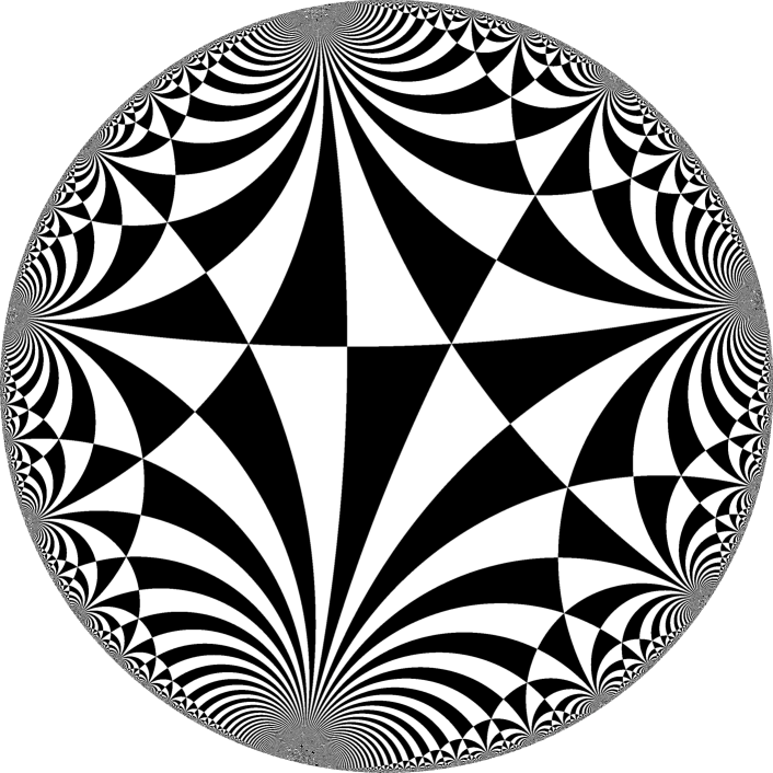
Figure 1: Poincaré disk model of fundamental domain triangles for the hyperbolic Coxeter group $[2,3,\infty]$

Denoting the phase-space coordinates by $(x^{\mu},p_{\mu})$ for $\mu=0,1,2$, the Minkowski metric by $\eta_{\mu\nu}$ and the Lorentzian scalar product again by ‘$\cdot$’, the Hamiltonian then has the form (employing the Einstein summation convention and pulling the coupling out of the potential)

$$H\ =\ \tfrac{1}{2}\eta^{\mu\nu}p_{\mu}p_{\nu}+\ g(g{-}1)\,V(x)\ =\ \tfrac{1}{2}\bigl{(}-p_{0}^{2}+p_{1}^{2}+p_{2}^{2}\bigr{)}\ +\ \tfrac{1}{2}\sum_{\alpha\in{\cal R}}\frac{g(g{-}1)}{(\alpha\cdot x)^{2}}\ ,$$ (1.5)

where the sum is restricted to the set $\cal R$ of real roots, which we normalize to $\alpha{\cdot}\alpha=2$. Since $\cal R$ for $AE_{3}$ decomposes into two Weyl orbits ${\cal R}_{+}$ and ${\cal R}_{-}$ [17], we may actually split the potential into two pieces and weigh them individually. However, for the sake of simplicity we keep the couplings equal for this paper, $g_{+}{=}g_{-}{=}g$. We also do not consider the possible inclusion of imaginary roots in the potential.

Like the Euclidean theory can be reduced to the unit sphere, the Minkowskian variant can be restricted to the one-sheeted hyperboloid ($x{\cdot}x=1$) or (one sheet of) the two-sheeted hyperboloid ($x{\cdot}x=-1$). In order to produce a model on a Riemannian manifold (with Euclidean signature), we consider the future hyperboloid $H^{2}$ given by $x{\cdot}x=-1$ and $x^{0}>1$. Let us parametrize the Minkowski future by

$$x^{0}=r\,\cosh\theta\ ,\quad x^{1}=r\,\sinh\theta\,\cos\phi\ ,\quad x^{2}=r\,\sinh\theta\,\sin\phi\quad\quad\textrm{with}\quad r\in\mathds{R}_{>0}\ ,\quad\theta\in\mathds{R}_{\geq 0}\ ,\quad\phi\in[0,2\pi]$$ (1.6)

so that we may restrict to $r{=}1$ and obtain the quantum Hamiltonian of a “hyperbolic Calogero model” 

$$H_{\Omega}\ =\ -\tfrac{1}{2}L^{2}+g(g{-}1)\,U(\theta,\phi)\quad\quad\textrm{with}\quad\quad L^{2}=\partial_{\theta}^{2}+\coth\theta\,\partial_{\theta}+\textrm{csch}^{2}\!\theta\,\partial_{\phi}^{2}\quad\quad\textrm{and}\quad\quad U(\theta,\phi)=r^{2}\,V(x)\ ,$$ (1.7)

where $L^{2}$ is just the (scalar) Laplacian on $H^{2}$. Our task will be to compute and characterize the potential $V$ respective $U$.

2 The real roots of the Kac–Moody algebra $AE_{3}$

In order to formulate the Calogero potential for the real roots of $AE_{3}$ we need to collect some facts about this simplest of hyperbolic Kac–Moody algebras [13, 12, 11]. Starting from its Cartan matrix,

$$A\ =\ \begin{pmatrix}\phantom{-}2&-2&\phantom{-}0\phantom{-}\\ -2&\phantom{-}2&-1\phantom{-}\\ \phantom{-}0&-1&\phantom{-}2\phantom{-}\end{pmatrix}\ ,$$ (2.1)

we parametrize the three simple roots $\alpha_{\mu}$ of length-square 2 in three-dimensional Minkowski space $\mathds{R}^{1,2}$ with a Minkowski-orthonormal basis $\{e_{\mu}\}=\{e_{0},e_{1},e_{2}\}$,

$$e_{\mu}{\cdot}\,e_{\nu}\ =\ \eta_{\mu\nu}\quad\quad\textrm{for}\quad\quad(\eta_{\mu\nu})=\textrm{diag}(-1,+1,+1)\ ,$$ (2.2)

via

$$\alpha_{0}\ =\ \sqrt{2}\,\bigl{(}\tfrac{1}{\sqrt{3}}e_{0}-e_{1}-\tfrac{1}{\sqrt{3}}e_{2}\bigr{)}\ ,\qquad\alpha_{1}\ =\ \sqrt{2}\,e_{1}\ ,\qquad\alpha_{2}\ =\ \sqrt{2}\,\bigl{(}-\tfrac{1}{2}e_{1}+\tfrac{1}{2}\sqrt{3}\,e_{2}\bigr{)}\ .$$ (2.3)

For symmetry reasons we add the non-simple root

$$\alpha_{3}\ =\ -\alpha_{1}{-}\alpha_{2}\ =\ \sqrt{2}\bigl{(}-\tfrac{1}{2}e_{1}-\tfrac{1}{2}\sqrt{3}\,e_{2}\bigr{)}\ ,$$ (2.4)

so that the overextended simple root can be rewritten as

$$\alpha_{0}\ =\ \sqrt{\tfrac{2}{3}}\,e_{0}-\tfrac{2}{3}\,\alpha_{1}+\tfrac{2}{3}\,\alpha_{3}\ .$$ (2.5)

The three roots $\alpha_{i}$, $i=1,2,3$, belong to an $A_{2}$ subalgebra and obey the relations

$$\alpha_{1}+\alpha_{2}+\alpha_{3}=0\ ,\qquad\alpha_{i}{\cdot}\,\alpha_{i}=2\ ,\qquad\alpha_{i}{\cdot}\,\alpha_{j}=-1\ (i{\neq}j)\ ,\qquad(\alpha_{i}-\alpha_{j}){\cdot}\,\alpha_{k}=0\ (i{\neq}k{\neq}j)\ .$$ (2.6)

The real roots of $AE_{3}$ lie on the one-sheeted hyperboloid $x{\cdot}x{=}2$ and are given by

$$\alpha\ =\ \ell\,\alpha_{0}+m\,\alpha_{1}+n\,\alpha_{2}\quad\quad\textrm{with}\quad\quad\ell,m,n\in\mathds{Z}\quad\quad\textrm{and}\quad\quad\alpha\cdot\alpha=2\ ,$$ (2.7)

where the length condition translates to the diophantine equation

$$(\ell-m)^{2}+n\,(n-m)\ =\ 1\ .$$ (2.8)

Since the roots come in pairs $(\alpha,-\alpha)$, it suffices to analyze $\ell\geq 0$ only. At any given “level” $\ell$ the solutions furnish (generically several) highest weights of the “horizontal” $A_{2}\equiv sl_{3}$ subalgebra plus their images under its $S_{3}$ Weyl-group action,

$$(m,n)\ \to\ (m,m{-}n)\ \to\ (2\ell{-}n,m{-}n)\ \to\ (2\ell{-}n,2\ell{-}m)\ \to\ (2\ell{-}m{+}n,2\ell{-}m)\ \to\ (2\ell{-}m{+}n,n)\ .$$ (2.9)

Such a sextet of weights belongs to an $A_{2}$ representation with Dynkin labels

$$[{\bar{p}},{\bar{q}}]\ =\ [-2\ell{+}2m{-}n,{-}m{+}2n]\qquad\Leftrightarrow\qquad(m,n)_{\textrm{hw}}\ =\ \tfrac{1}{3}\,(4\ell{+}2{\bar{p}}{+}{\bar{q}},2\ell{+}{\bar{p}}{+}2{\bar{q}})$$ (2.10)

for the highest-weight values $(m,n)_{\textrm{hw}}$ in (2.9). Fig. 2 shows the distribution of the real roots for low levels.

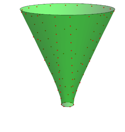
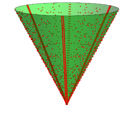
Figure 2: Hyperboloid $x{\cdot}x=2$ (green) and real roots $\alpha$ (red) for $0\leq\ell\leq 12$ (left) and $0\leq\ell\leq 122$ (right)

We obtain a parametrization more symmetric under spatial rotations by replacing $\alpha_{0}$ with $e_{0}$ using (2.5) and employing a kind of barycentric coordinates,

$$x\ =\ x^{0}\,e_{0}+\bar{x}^{i}\,\alpha_{i}\qquad\quad\textrm{with}\quad\quad\bar{x}^{1}{+}\bar{x}^{2}{+}\bar{x}^{3}=0\ .$$ (2.11)

In these coordinates, the real roots take the form

$$\alpha\ =\ \sqrt{\tfrac{2}{3}}\,\ell\,e_{0}+\bar{\alpha}\quad\quad\textrm{with}\quad\quad\bar{\alpha}\ =\ \tfrac{1}{3}{\bar{p}}\,\alpha_{1}+\tfrac{1}{3}{\bar{q}}\,\alpha_{2}+\tfrac{1}{3}{\bar{r}}\,\alpha_{3}\quad\quad\textrm{and}\quad\quad{\bar{p}}+{\bar{q}}+{\bar{r}}=0\ ,$$ (2.12)

where ${\bar{p}}$ and ${\bar{q}}$ coincide with the Dynkin labels in case $\bar{\alpha}$ is a highest $A_{2}$ weight. The $S_{3}$ Weyl group action simply permutes the coefficients $({\bar{p}},{\bar{q}},{\bar{r}})$ and multiplies them with the sign of the permutation. On a given level $\ell$ the $A_{2}$ weights $\bar{\alpha}$ all have the same length-square $\bar{\alpha}{\cdot}\bar{\alpha}=2+\tfrac{2}{3}\ell^{2}$. On may translate the diophantine equation (2.8) to the Dynkin labels and obtain

$$-{\bar{p}}{\bar{q}}-{\bar{p}}{\bar{r}}-{\bar{r}}{\bar{p}}\ \equiv\ {\bar{p}}^{2}+{\bar{q}}^{2}+{\bar{p}}\,{\bar{q}}\ =\ \ell^{2}+3\qquad\textrm{as well as}\qquad 3\mid\ell-{\bar{p}}+{\bar{q}}\ .$$ (2.13)

The number of $A_{2}$ representations grows erratically with the level, as displayed in Fig. 3. Two representations appear first at $\ell{=}6$, three at $\ell{=}12$, four at $\ell{=}30$, eight at $\ell{=}72$ and so on.

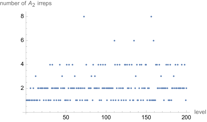
Figure 3: Multiplicity of $A_{2}$ representations occurring at level $\ell$

At level zero one simply finds the adjoint representation,

$$\ell=0:\qquad(m,n)_{\textrm{hw}}=(1,1)\qquad\Leftrightarrow\qquad[{\bar{p}},{\bar{q}}]=[1,1]\ .$$ (2.14)

Although the number of solutions grows quickly with $\ell$ it is easy to give a few infinite families of real roots (see also [11]),

$$\ell\geq 1: (m,n)_{\textrm{hw}}=(2\ell,\ell{+}1)\qquad \Leftrightarrow \qquad[{\bar{p}},{\bar{q}}]=[\ell{-}1,2]\ ,$$ (2.15)

$$\ell=3k\geq 3: (m,n)_{\textrm{hw}}=(5k{+}1,4k)\qquad \Leftrightarrow \qquad[{\bar{p}},{\bar{q}}]=[2,3k{-}1]\ ,$$

$$\ell=k(k{+}1)\geq 6: (m,n)_{\textrm{hw}}=(2k(k{+}1){-}1,k(k{+}2))\qquad \Leftrightarrow \qquad[{\bar{p}},{\bar{q}}]=[k^{2}{-}2,2k{+}1]\ ,$$

where at $\ell{=}6$ the second and third series coincide for $k{=}2$, the $k{=}1$ solution is contained in the first series at $\ell{=}3$, and the $\ell{=}1$ solution is degenerate under the Weyl group action,

$$(m,n)=(2,2),(2,0),(0,0)\qquad\Leftrightarrow\qquad[{\bar{p}},{\bar{q}}]=[0,2]\ .$$ (2.16)

With increasing level the real roots hug the lightcone, as is apparent from Fig. 4.

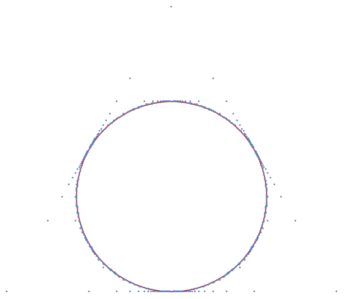
Figure 4: Projective view $\tfrac{\alpha}{|\alpha{\cdot}e_{0}|}-e_{0}$ of the real roots $\alpha$ for $1\leq\ell\leq 100$ (the red circle is the lightcone)

The roots of the first family are also neatly expressed as

$$\alpha\ =\ \ell\,n_{i}\pm\alpha_{i}\quad\quad\textrm{for}\quad\quad i=1,2,3\qquad\quad\textrm{with}\quad\quad\alpha_{\textrm{hw}}=\ell\,n_{2}+\alpha_{2}$$ (2.17)

in terms of a triplet of null vectors

$$n_{1} \ =\ \alpha_{0}-\alpha_{2}-\alpha_{3}\ =\ \sqrt{\tfrac{2}{3}}\,e_{0}+\tfrac{1}{3}(\alpha_{3}-\alpha_{2})\ =\ \sqrt{2}\,\bigl{(}\tfrac{1}{\sqrt{3}}e_{0}-\tfrac{1}{\sqrt{3}}e_{2}\bigr{)}\ ,$$ (2.18)

$$n_{2} \ =\ \alpha_{0}+\alpha_{1}-\alpha_{3}\ =\ \sqrt{\tfrac{2}{3}}\,e_{0}+\tfrac{1}{3}(\alpha_{1}-\alpha_{3})\ =\ \sqrt{2}\,\bigl{(}\tfrac{1}{\sqrt{3}}e_{0}+\tfrac{1}{2}e_{1}+\tfrac{1}{2\sqrt{3}}e_{2}\bigr{)}\ ,$$

$$n_{3} \ =\ \alpha_{0}+\alpha_{1}+\alpha_{2}\ =\ \sqrt{\tfrac{2}{3}}\,e_{0}+\tfrac{1}{3}(\alpha_{2}-\alpha_{1})\ =\ \sqrt{2}\,\bigl{(}\tfrac{1}{\sqrt{3}}e_{0}-\tfrac{1}{2}e_{1}+\tfrac{1}{2\sqrt{3}}e_{2}\bigr{)}\ ,$$

which satisfy the relations

$$n_{i}{\cdot}\,n_{i}=0\ ,\quad n_{i}{\cdot}\,n_{j}=-1\ (i{\neq}j)\ ,\quad\alpha_{i}{\cdot}\,n_{j}={\textstyle\sum}_{k}\epsilon_{ijk}\ ,\quad n_{1}{+}n_{2}{+}n_{3}=\sqrt{6}\,e_{0}\ ,\quad(\ell\,n_{i}\pm\alpha_{i})^{2}=2\ .$$ (2.19)

Since the real roots

$$\alpha\ =\ \sqrt{2}\bigl{(}\sinh\eta\,e_{0}\ +\ \cosh\eta\cos\chi\,e_{1}\ +\ \cosh\eta\sin\chi\,e_{2}\bigr{)}$$ (2.20)

are spacelike and located on a one-sheeted hyperboloid, the fix planes of the corresponding reflections $s_{\alpha}$,

$$\alpha{\cdot}x\ =\ 0\qquad\Leftrightarrow\qquad\tanh\eta\ =\ \tanh\theta\,\cos(\chi{-}\phi)\ ,$$ (2.21)

are timelike planes through the origin, which we call “mirrors”. They intersect the lightcone and the two-sheeted hyperboloid $x{\cdot}x=-1$. The reflections $s_{\alpha}$ act on the Minkowskian components $x^{\mu}$ of a point $x$ as $(s_{\alpha}x)^{\mu}=S^{\mu}_{\ \nu}x^{\nu}$ with

$$\bigl{(}S^{\mu}_{\ \nu}\bigr{)}\ =\ \begin{pmatrix}1&0&0\\ 0&\cos\chi&-\sin\chi\\ 0&\sin\chi&\cos\chi\end{pmatrix}\begin{pmatrix}\cosh 2\eta&-\sinh 2\eta&0\\ \sinh 2\eta&-\cosh 2\eta&0\\ 0&0&1\end{pmatrix}\begin{pmatrix}1&0&0\\ 0&\cos\chi&\sin\chi\\ 0&-\sin\chi&\cos\chi\end{pmatrix}\ .$$ (2.22)

Each such hyperbolic reflection preserves the radial coordinate $r=\sqrt{-x{\cdot}x}$ and the time orientation but reverses the spatial orientation ($\det S=-1$), hence it represents an involution on the future hyperboloid. A collection of such mirrors is displayed in Fig. 5, and Fig. 6 shows their intersections with the $x^{0}{=}1$ plane.

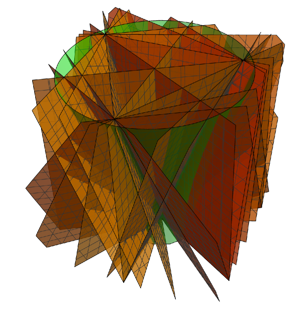
Figure 5: The real-root mirrors for levels $|\ell|\leq 3$ (the green hyperboloid is $x{\cdot}x=2$)

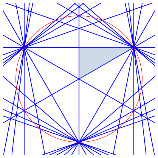
Figure 6: Intersection of the mirror planes (blue) for $|\ell|\leq 5$ and the lightcone (red) with the $x^{0}{=}1$ plane. The standard fundamental alcove is shaded.

3 The potential

The “horizontal” $A_{2}$ slicing of the root space into levels $\ell\in\mathds{Z}$ leads to a decomposition of the potential,

$$V(x)\ =\ \sum_{\ell\in\mathds{Z}}V_{\ell}(x)\qquad\quad\textrm{with}\quad\quad V_{\ell}(x)\ =\ \tfrac{1}{2}\sum_{\alpha\in{\cal R}_{\ell}}\frac{1}{(\alpha\cdot x)^{2}}\ ,$$ (3.1)

where ${\cal R}_{\ell}$ denotes the set of real roots $\alpha$ with $\alpha{\cdot}e_{0}=\sqrt{\tfrac{2}{3}}\,\ell$. Clearly, $V_{-\ell}=V_{\ell}$.

Let us take a look at levels zero and one. Summing over the adjoint representation of $A_{2}$,

$$V_{0}(r,\theta,\phi)\ =\ \sum_{i=1,2,3}\frac{1}{(\alpha_{i}\cdot x)^{2}}\ =\ \frac{\mathrm{csch}^{\!2}\theta}{2\,r^{2}}\biggl{(}\frac{1}{\cos^{2}\!\phi}+\frac{1}{\cos^{2}(\phi{-}\tfrac{2\pi}{3})}+\frac{1}{\cos^{2}(\phi{+}\tfrac{2\pi}{3})}\biggr{)}\ =\ \frac{9}{2\,r^{2}}\,\frac{\mathrm{csch}^{\!2}\theta}{\cos^{2}\!3\phi}$$ (3.2)

is just the celebrated Pöschl–Teller potential, modulated by a $\theta$ dependence. For level one we sum over the three extremal weights of the $[0,2]$ representation,

$$V_{1}(r,\theta,\phi)\ =\ \sum_{i=1,2,3}\frac{1}{([n_{i}{+}\alpha_{i}]\cdot x)^{2}}$$ (3.3)

$$\ =\ \frac{3}{2\,r^{2}}\biggl{(}\frac{1}{(\cosh\theta+2\sinh\theta\sin\phi)^{2}}+\frac{1}{(\cosh\theta+2\sinh\theta\sin(\phi{-}\tfrac{2\pi}{3}))^{2}}+\frac{1}{(\cosh\theta+2\sinh\theta\sin(\phi{+}\tfrac{2\pi}{3}))^{2}}\biggr{)}$$

$$\ =\ \frac{18}{r^{2}}\,\frac{\cosh^{4}\!\theta+3\sinh^{4}\!\theta+4\cosh\theta\sinh^{3}\!\theta\sin 3\phi}{(\cosh 3\theta-3\cosh\theta+4\sinh^{3}\!\theta\sin 3\phi)^{2}}\ .$$

It is also possible to sum over whole families of solutions to the diophantine equation (2.8). Let us do so for the first family in (2.15), extending it to negative levels (to include the negative real roots) and including levels zero and one with their proper weight inside $V$,

$$V_{\textrm{1st family}} \ =\ -V_{0}-V_{1}+\ \sum_{\ell=0}^{\infty}\sum_{i=1,2,3}\biggl{(}\frac{1}{([\ell\,n_{i}{+}\alpha_{i}]\cdot x)^{2}}+\frac{1}{([\ell\,n_{i}{-}\alpha_{i}]\cdot x)^{2}}\biggr{)}$$ (3.4)

$$\ =\ -V_{0}-V_{1}+\sum_{i=1,2,3}\frac{2}{(n_{i}{\cdot}x)^{2}}\ \sum_{\ell=0}^{\infty}\frac{\ell^{2}+\bigl{(}\tfrac{\alpha_{i}{\cdot}x}{n_{i}{\cdot}x}\bigr{)}^{2}}{\bigl{[}\ell^{2}-\bigl{(}\tfrac{\alpha_{i}{\cdot}x}{n_{i}{\cdot}x}\bigr{)}^{2}\bigr{]}^{2}}$$

$$\ =\ -V_{0}-V_{1}+\sum_{i=1,2,3}\frac{1}{(n_{i}{\cdot}x)^{2}}\ \biggl{(}\frac{1}{\bigl{(}\tfrac{\alpha_{i}{\cdot}x}{n_{i}{\cdot}x}\bigr{)}^{2}}+\frac{\pi^{2}}{\sin^{2}\!\bigl{(}\pi\tfrac{\alpha_{i}{\cdot}x}{n_{i}{\cdot}x}\bigr{)}}\biggr{)}$$

$$\ =\ \sum_{i=1,2,3}\biggl{(}\frac{\pi^{2}}{(n_{i}{\cdot}x)^{2}\sin^{2}\!\bigl{(}\pi\tfrac{\alpha_{i}{\cdot}x}{n_{i}{\cdot}x}\bigr{)}}\ -\ \frac{1}{([n_{i}{+}\alpha_{i}]\cdot x)^{2}}\biggr{)}\ ,$$

where the $V_{0}$ contribution got cancelled on the way. Although this is only a part of the full potential, it does show some characteristic features of $V$:

• the $A_{2}$ subgroup’s Weyl group $S_{3}$ yields a dihedral symmetry and six-fold mirrors,

• infinitely many mirrors intersect in the three null lines $\lambda n_{i}$,

• in the $\ell\to\infty$ limit the mirrors accumulate in the three null planes $n_{i}{\cdot}x=0$.

• the mirrors tessalate the interior of the lightcone with infinitely many triangular Weyl alcoves

• a fundamental Weyl alcove is spanned by $\{e_{0},2e_{0}{+}e_{2},2e_{0}{+}\sqrt{3}e_{1}{+}e_{2}\}$

A contour plot of $\log V$ on the plane $x^{0}{=}1$ is given in Fig. 7 for one Weyl alcove.

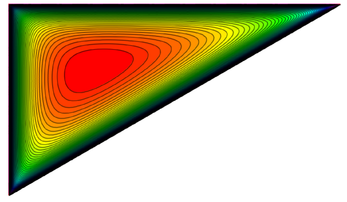
Figure 7: Contour lines of $\log V$ for the standard fundamental alcove intersecting the $x^{0}{=}1$ plane

4 Mapping to the complex half-plane

Since our model is scale invariant, for the potential we can restrict ourselves to the future hyperboloid $r^{2}=-x{\cdot}x=1$ and $x^{0}\geq 1$. It is convenient to pass to complex embedding coordinates

$$t=x^{0}\quad\textrm{and}\quad w=x^{1}+\mathrm{i}x^{2}\qquad\quad\textrm{with}\quad\quad t^{2}-\bar{w}w=1\ .$$ (4.1)

By a stereographic projection (see Fig. 8) the hyperboloid gets mapped to the unit disk $\bar{v}v\leq 1$ for $v\in\mathds{C}$,

$$\frac{w}{t{+}1}=\frac{v}{1}\qquad\Rightarrow\qquad w=\frac{2v}{1-\bar{v}v}\ ,\quad v=\frac{w}{1+\sqrt{1{+}\bar{w}w}}\ ,\quad t=\frac{1+\bar{v}v}{1-\bar{v}v}\ .$$ (4.2)

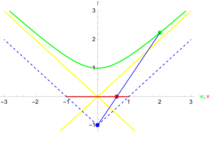
Figure 8: Stereographic projection of the hyperboloid (green) to the disk (red), with the lightcone (yellow)

The metric induced from the Minkowski metric turns this into the Poincaré disk model of the hyperbolic plane $H^{2}$. The intersection curves with the mirrors of level zero and one are easily computed as

$$\ell=0: \qquad\,v+\bar{v}=0\ ,\qquad\quad\ \bar{\rho}\,v+\rho\,\bar{v}=0\ ,\qquad\ \rho\,v+\bar{\rho}\,\bar{v}=0\ ,$$ (4.3)

$$\ell=1: \qquad|v-2\mathrm{i}|^{2}=3\ ,\qquad|v-2\mathrm{i}\rho|^{2}=3\ ,\qquad|v-2\mathrm{i}\bar{\rho}|^{2}=3\ ,$$

where

$$\rho=\mathrm{e}^{2\pi\mathrm{i}/3}\qquad\Rightarrow\qquad\rho^{2}=\bar{\rho}\ ,\quad\rho+\bar{\rho}=-1\ ,\quad 1+\rho+\rho^{2}=0\ .$$ (4.4)

Adding the infinity of real-root mirrors produces a paracompact triangular tessalation of type $[p,q,r]=[2,3,\infty]$. Each of the hyperbolically congruent triangles has angles $\frac{\pi}{2}$, $\frac{\pi}{3}$ and $0$, and at the corresponding vertices there meet 4, 6 and infinitely many triangles, thus one vertex is always at the boundary, as is visible from Fig. 9.

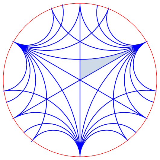
Figure 9: The mirror lines (blue) for $|\ell|\leq 5$ in the Poincaré disk $\bar{v}v{<}1$ (with red boundary $\bar{v}v{=}1$)

We employ a variant of the Cayley map to further pass to the complex upper half plane ${\cal H}\ni z$,

$$v=-\mathrm{i}\,\frac{\rho\,z+1}{z+\rho}\qquad\Leftrightarrow\qquad z=\frac{1-\mathrm{i}\rho\,v}{\mathrm{i}\,v-\rho}\ ,$$ (4.5)

such that the boundary $|v|{=}1$ becomes the real axis $\textrm{Im}\,z{=}0$. The direct relation between $w$ and $z$ reads

$$w\ =\ \frac{2}{\sqrt{3}}\,\frac{(1{+}\rho\,z)(\bar{\rho}{+}\bar{z})}{z-\bar{z}}\ =\ \frac{2}{\sqrt{3}}\,\frac{\rho\,z\bar{z}+(z{+}\bar{z})+\bar{\rho}}{z-\bar{z}}\ =\ \frac{2\,\rho}{\sqrt{3}}\,\frac{(z{+}\bar{\rho})(\bar{z}{+}\bar{\rho})}{z-\bar{z}}\ ,$$ (4.6)

and the mirror curves at level zero and one become (in the same order as in (4.3))

$$\ell=0: \qquad z\,{\bar{z}}=1\ ,\qquad\quad\ z+{\bar{z}}=1\ ,\qquad\qquad\quad\ (z{-}1)({\bar{z}}{-}1)=1\ ,$$ (4.7)

$$\ell=1: \qquad z+{\bar{z}}=0\ ,\qquad(2z{-}1)(2{\bar{z}}{-}1)=1\ ,\qquad z+{\bar{z}}=2\ .$$

The first two curves in the $\ell{=}0$ list and the first one at $\ell{=}1$ bound a standard fundamental domain

$${\cal F}\ =\ \bigl{\{}z\in{\cal H}\ \bigm{|}\ |z|\geq 1\quad\textrm{and}\quad 0\leq\Re\,z\leq\tfrac{1}{2}\bigr{\}}\ ,$$ (4.8)

which is co-finite (with a hyperbolic volume of $\tfrac{\pi}{6}$) but not co-compact due to a cusp at $\mathrm{i}\infty$. Fig. 10 shows the mirror lines of Fig. 9 mapped to the upper half plane $\cal H$.

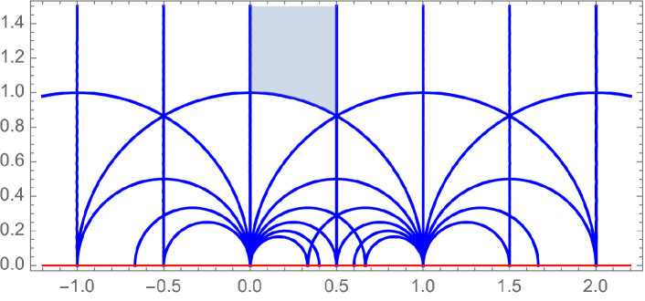
Figure 10: The mirror lines (blue) for $|\ell|\leq 5$ in the upper half plane $\Im\,z>0$ (with red boundary $\Im\,z=0$)

Any other triangle in the tessalation is reached by applying a suitable element of PGL($2,\mathds{Z}$), the group of integral $2{\times}2$ matrices with determinant $+1$ or $-1$ modulo $\{\pm\mathbbm{1}\}$:

$$z\ \mapsto\ \begin{cases}\ \tfrac{az+b}{cz+d}&\textrm{if}\quad\bigl{|}\begin{smallmatrix}a&b\\ c&d\end{smallmatrix}\bigr{|}=+1\\[4.0pt] \ \tfrac{a{\bar{z}}+b}{c{\bar{z}}+d}&\textrm{if}\quad\bigl{|}\begin{smallmatrix}a&b\\ c&d\end{smallmatrix}\bigr{|}=-1\end{cases}\qquad\quad\textrm{with}\quad a,b,c,d\in\mathds{Z}\ .$$ (4.9)

This happens to be the Weyl group of our hyperbolic Kac-Moody algebra. It can be generated by the three reflections

$$s_{1}=s_{\alpha_{1}}:\quad z\mapsto 1/{\bar{z}}\ ,\qquad s_{2}=s_{\alpha_{2}}:\quad z\mapsto 1{-}{\bar{z}}\ ,\qquad s_{3}=s_{\alpha_{0}-2\alpha_{3}}:\quad z\mapsto-{\bar{z}}\ ,$$ (4.10)

whose fixpoints form the three mirror curves mentioned above, which bound the fundamental triangle (4.8). The two generators of the even subgroup PSL($2,\mathds{Z}$) are

$$T=s_{2}s_{3}:\quad z\mapsto z{+}1\quad\quad\textrm{and}\quad\quad S=s_{1}s_{3}:\quad z\mapsto-1/z\ ,$$ (4.11)

and its standard fundamental domain is cut in half by the extra reflection $s_{3}$. In matrix representation $(\begin{smallmatrix}a&b\\ c&d\end{smallmatrix})$ we have

$$s_{1}\mathrel{\widehat{=}}(\begin{smallmatrix}0&1\\ 1&0\end{smallmatrix})\ ,\qquad s_{2}\mathrel{\widehat{=}}(\begin{smallmatrix}1&-1\\ 0&-1\end{smallmatrix})\ ,\qquad s_{3}\mathrel{\widehat{=}}(\begin{smallmatrix}1&0\\ 0&-1\end{smallmatrix})\ ,\qquad T\mathrel{\widehat{=}}(\begin{smallmatrix}1&1\\ 0&1\end{smallmatrix})\ ,\qquad S\mathrel{\widehat{=}}(\begin{smallmatrix}0&-1\\ 1&0\end{smallmatrix})\ ,$$ (4.12)

up to multiplication by $-1$ of course. The simple-root reflection $s_{\alpha_{0}}:z\mapsto\frac{{\bar{z}}}{2{\bar{z}}-1}$ appears in the middle of our $\ell{=}1$ lists (4.3) and (4.7). Choosing it instead of $s_{3}$ leads to a fundamental domain with the cusp sitting at $1$ rather than $\mathrm{i}\infty$. In any case, it is clear that the potential $U(z)=V\bigl{(}r{=}1,\theta(z),\phi(z)\bigr{)}$ is a real automprphic function with respect to PGL($2,\mathds{Z}$). We end this section by displaying $\log U$ in the Poincaré disk and in the upper half plane for the standard fundamental domain in Fig. 11.

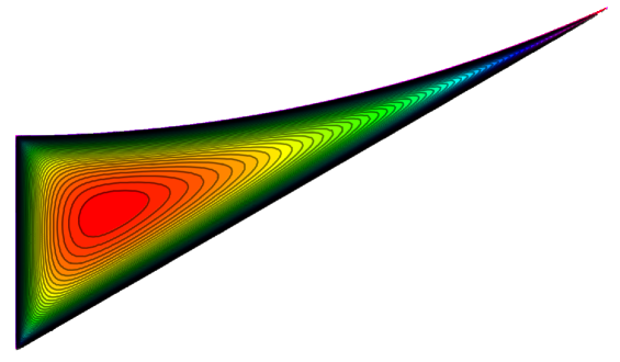
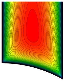
Figure 11: Contour lines of $\log U$ for a fundamental domain in the $v$ disk (left) and the $z$ plane (right)

5 The potential as a Poincaré series

Our potential is a sum over all real roots $\alpha$ of $AE_{3}$, thus each reflection $s_{\alpha}$ inside PGL($2,\mathds{Z}$) provides one summand. These reflections are given by traceless matrices $R$ of determinant $-1$,

$$s_{\alpha}\equiv s_{R}\ :\quad z\ \mapsto\ \frac{p{\bar{z}}+q}{r{\bar{z}}-p}\qquad\quad\textrm{with}\quad\quad R=\begin{pmatrix}p&q\\[2.0pt] r&-p\end{pmatrix}\quad\quad\textrm{and}\quad\quad p^{2}+q\,r=1\ .$$ (5.1)

The scalar product in root space is an invariant bilinear form,

$$\alpha{\cdot}\alpha^{\prime}\ =\ \mathrm{tr}(s_{\alpha}\,s_{\alpha^{\prime}})\ =\ 2\,p\,p^{\prime}+q\,r^{\prime}+r\,q^{\prime}\ \in\mathds{Z}\ .$$ (5.2)

From (4.6) we see that the real function $\alpha{\cdot}x$ odd under $s_{\alpha}$ becomes a real quadratic polynomial in $z$ and ${\bar{z}}$ divided by $|z{-}{\bar{z}}|$. A quick computation shows that

$$\alpha{\cdot}x\ =\ \tfrac{\sqrt{2}\,\mathrm{i}}{z-{\bar{z}}}\,\bigl{[}r\,z\,{\bar{z}}-p(z{+}{\bar{z}})-q\bigr{]}$$ (5.3)

is indeed odd under the reflection (5.1). Therefore, on the upper half plane the potential is expressed as

$$U(z)\equiv V\bigl{(}x(z)\bigr{)}\ =\ \frac{1}{4}\sum_{R}\frac{|z-{\bar{z}}|^{2}}{[r\,z\,{\bar{z}}-p(z{+}{\bar{z}})-q]^{2}}\ =\ \frac{1}{4}\sum_{R}\frac{4\,y^{2}}{[r(x^{2}{+}y^{2})-2p\,x-q]^{2}}\ =:\ \frac{1}{4}\sum_{R}u_{R}(z)$$ (5.4)

where $z=x+\mathrm{i}\,y$ and the sum runs over all reflections $R$ in (5.1), with $R$ and $-R$ contributing the same. Comparison with

$$-\alpha{\cdot}x\ =\ \tfrac{\sqrt{2}\,\mathrm{i}}{z-{\bar{z}}}\,\bigl{[}(2\ell{-}m)\,z{\bar{z}}+(n{-}\ell)(z{+}{\bar{z}})+(m{-}n)\bigr{]}$$ (5.5)

provides the translation between the labels $(p,q,r)$ and $(\ell,m,n)$, up to a common sign of course. As an aside, we characterize in the following table the two orbits (e for $\ell$ even, o for $\ell$ odd) of the Weyl group on the set $\cal R$ of real roots.

	$\ell$	$m$	$n$	$p$	$q$	$r$
	e	o	o	o	e	o
${\cal R}_{+}$	e	e	o	o	o	e
	e	o	e	e	o	o
${\cal R}_{-}$	o	e	e	o	e	e

Restricting our potential to one of the two Weyl orbits removes either the $\ell{=}\textrm{odd}$ or the $\ell{=}\textrm{even}$ mirror lines from all diagrams and doubles the fundamental domain. In an Appendix with Don Zagier we outline how far one can proceed with an explicit computation of the potential function $U(z)$.

The potential $U(z)$ is a real modular function under the action of GL($2,\mathds{Z}$), which is manifest via

$$u_{R}(Mz)\ =\ u_{M^{-1}R\,M}(z)\qquad\quad\textrm{for}\quad\quad Mz=\tfrac{az+b}{cz+d}\quad\quad\textrm{with}\quad\quad a,b,c,d\in\mathds{Z}\ .$$ (5.6)

Hence, we can replace the sum over $R$ with sums over appropriate orbits by the adjoint action of GL($2,\mathds{Z}$) for a suitable reference, say

$$R_{0}\ =\ \bigl{(}\begin{smallmatrix}1&0\\[2.0pt] 0&-1\end{smallmatrix}\bigr{)}\qquad\Leftrightarrow\qquad z\ \mapsto\ -{\bar{z}}\qquad\Leftrightarrow\qquad u_{R_{0}}(z)=\frac{y^{2}}{x^{2}}=:u(z)\ ,$$ (5.7)

and obtain 

$$2\,U(z)\ =\ \frac{1}{4}\sum_{M}u_{M^{-1}R_{0}M}(z)\ =\ \frac{1}{4}\sum_{M}u(Mz)\ =\ \frac{1}{4}\sum_{M}\frac{(ad{-}bc)^{2}\ y^{2}}{[ac(x^{2}{+}y^{2})+(ad{+}bc)x+bd]^{2}}\ .$$ (5.8)

The question is: over which subset of GL($2,\mathds{Z}$) matrices does this sum run? Since our fundamental domain ${\cal F}$ in (4.8) is half of the standard one for PSL($2,\mathds{Z}$), all reflections $R$ should be covered using adjoint orbits by matrices $M_{n}$ of determinant $n=ad{-}bc$ equal to one or two. Indeed, for $R\in{\cal R}_{+}$, we can find a unique (up to sign and the footnote) matrix $M_{2}$ such that $R=M_{2}^{-1}R_{0}M_{2}$. In the case of $R\in{\cal R}_{-}$, in constrast, there are two such matrices $M_{2}$, which have the form

$$\Bigl{(}\begin{smallmatrix}2a^{\prime}&2b^{\prime}\\[4.0pt] c^{\prime}&d^{\prime}\end{smallmatrix}\Bigr{)}\quad\quad\textrm{and}\quad\quad\Bigl{(}\begin{smallmatrix}a^{\prime}&b^{\prime}\\[4.0pt] 2c^{\prime}&2d^{\prime}\end{smallmatrix}\Bigr{)}\qquad\Rightarrow\qquad\det\Bigl{(}\begin{smallmatrix}a^{\prime}&b^{\prime}\\[4.0pt] c^{\prime}&d^{\prime}\end{smallmatrix}\Bigr{)}=1\ ,$$ (5.9)

so such reflections $R$ are covered twice by summing over $M_{2}$. However, they also make up (again uniquely) the $M_{1}$ orbit of $R_{0}$. Therefore, we can correct the overcount by subtracting,

$$2\,U(z)\ =\ F_{2}(z)-F_{1}(z)\qquad\quad\textrm{for}\quad\qquad F_{n}(z)\ :=\ \tfrac{1}{4}\sum_{M_{n}}u(Mz)\ .$$ (5.10)

The function $F_{2}$ can be obtained from $F_{1}$ by applying a Hecke operator $T_{2}$ (for weight $k{=}0$),

$$F_{2}(z)\ =\ (T_{2}F_{1})(z)\ =\ \sum_{\genfrac{}{}{0.0pt}{2}{ad=2}{a,d>0}}\sum_{b\,(\textrm{mod}\,d)}F_{1}\bigl{(}\tfrac{az+b}{d}\bigr{)}\ =\ F_{1}(2z)+F_{1}(\tfrac{z}{2})+F_{1}(\tfrac{z+1}{2})\ ,$$ (5.11)

and thus we have

$$2\,U(z)\ =\ F_{1}(2z)+F_{1}(\tfrac{z}{2})+F_{1}(\tfrac{z+1}{2})-F_{1}(z)\ .$$ (5.12)

Therefore, it suffices to compute the Poincaré series

$$F_{1}(z)\ =\ \tfrac{1}{4}\!\!\!\!\!\!\sum_{M\in\textrm{SL}(2,\mathds{Z})}\!\!\!\!u(Mz)\ .$$ (5.13)

There is another path to this result, which provides a useful connection to binary quadratic forms. Let us define [18]

$$\widetilde{F}_{D}(z)\ =\ \frac{1}{2}\sum_{Q(D)}\frac{D\ y^{2}}{[A(x^{2}{+}y^{2})+B\,x+C]^{2}}\ =\ \frac{1}{2}\sum_{Q(D)}\frac{D\ y^{2}}{|A\,z^{2}+B\,z+C|^{2}-y^{2}}\ ,$$ (5.14)

where $Q(D)$ denotes the set of binary quadratic forms $As^{2}{+}Bst{+}Ct^{2}$ over $\mathds{Z}$ with discriminant $D=B^{2}{-}4AC$. For $D{=}1$ there is a bijection between $Q(1)$ and PSL($2,\mathds{Z}$) by solving

$$a\,c=A\ ,\qquad b\,d=C\ ,\qquad a\,d={\textstyle\frac{1}{2}}(B{+}1)\ ,\qquad b\,c={\textstyle\frac{1}{2}}(B{-}1)\ .$$ (5.15)

We conclude that $\widetilde{F}_{1}=F_{1}$. For $D{=}4$ we have a bijection between $Q(4)$ and our reflections $R$ in (5.1),

$$r=A\ ,\qquad-2p=B\ ,\qquad-q=C\ .$$ (5.16)

Therefore, the potential can also be expressed as

$$2\,U(z)\ =\ \widetilde{F}_{4}(z)\ =\ \frac{1}{2}\sum_{Q(4)}\frac{4\ y^{2}}{[A(x^{2}{+}y^{2})+B\,x+C]^{2}}\ .$$ (5.17)

Now, $Q(4)$ can be reduced to $Q(1)$, and it is not too hard to check that indeed [18]

$$\widetilde{F}_{4}(z)\ =\ (T_{2}\widetilde{F}_{1})(z)-\widetilde{F}_{1}(z)\ =\ \widetilde{F}_{1}(2z)+\widetilde{F}_{1}(\tfrac{z}{2})+\widetilde{F}_{1}(\tfrac{z+1}{2})-\widetilde{F}_{1}(z)\ ,$$ (5.18)

confirming (5.12). It thus suffices to compute the generalized real-analytic Eisenstein series

$$\widetilde{F}_{1}(z)\ =\ \frac{1}{2}\sum_{Q(1)}\frac{y^{2}}{[A(x^{2}{+}y^{2})+B\,x+C]^{2}}\ =\ \frac{1}{2}\sum_{Q(1)}\frac{y^{2}}{|A\,z^{2}+B\,z+C|^{2}-y^{2}}\ ,$$ (5.19)

where $Q(1)$ indicates a discriminant $B^{2}-4AC=1$. As was shown in [18], this sum converges almost everywhere. However, it does not decay at $\mathrm{i}\infty$, but grows as $\widetilde{F}_{1}(x{+}\mathrm{i}y)\sim y^{2}$ for $y\to\infty$.

The form (5.17) can be translated back to the unit hyperboloid and indeed the Minkowski future, with the result

$$V(x)\ =\ \sum_{Q(4)}\frac{3}{\bigl{[}(2A{-}B{+}2C)\,x^{0}+\sqrt{3}(A{-}C)\,x^{1}-(A{-}2B{+}C)\,x^{2}\bigr{]}^{2}}\ ,$$ (5.20)

where the sum runs over all integers $A$, $B$ and $C$ subject to the $Q(4)$ condition $B^{2}-4AC=4$. In this way, the real roots are parametrized by binary quadratic forms, which is of course equivalent to the solutions of the diophantine equation (2.8) but may be more convenient or manageable.

6 Dunkl operators

Calogero models in a Euclidean space are known to be maximally superintegrable. This is also the case for the spherical reduction of the rational models. One key instrument to establish this property is the Dunkl operators [19]

$${\cal D}_{i}\ =\ \partial_{i}\ -\ \tfrac{g}{2}\sum_{\alpha\in\cal R}\frac{\alpha_{i}}{\alpha{\cdot}x}\,s_{\alpha}\qquad\textrm{for}\quad i=1,\ldots,n$$ (6.1)

and their angular versions

$${\cal L}_{ij}\ =\ x^{i}{\cal D}_{j}-x^{j}{\cal D}_{i}\ ,$$ (6.2)

respectively. Their crucial property is the commutation $[{\cal D}_{i},{\cal D}_{j}]=0$, while the ${\cal L}_{ij}$ deform the angular momentum algebra to a subalgebra of a rational Cherednik algebra [20]. It is known that every Weyl-invariant polynomial in the ${\cal D}_{i}$ or in the ${\cal L}_{ij}$ will, upon its restriction ‘res’ to Weyl-invariant functions, provide a conserved quantity, i.e. an operator which commutes with the Hamiltonian $H$ or $H_{\Omega}$, respectively. Indeed, the Hamiltonians themselves can be expressed in this way,

$$-2\,H \ =\ \textrm{res}\sum_{i=1}^{n}{\cal D}_{i}^{2}\ =\ \sum_{i=1}^{n}\partial_{i}^{2}-\textrm{res}\sum_{\alpha\in{\cal R}}\frac{\alpha{\cdot}\alpha}{2(\alpha{\cdot}x)^{2}}\,g(g{-}s_{\alpha})\ ,$$ (6.3)

$$-2\,H_{\Omega} \ =\ \textrm{res}\sum_{i<j}{\cal L}_{ij}^{2}-2E_{0}\ =\ L^{2}-\textrm{res}\sum_{\alpha\in{\cal R}}\frac{\alpha{\cdot}\alpha\,x{\cdot}x}{2(\alpha{\cdot}x)^{2}}\,g(g{-}s_{\alpha})\ ,$$

with the ground-state energy

$$E_{0}\ =\ \tfrac{1}{2}\,\textrm{res}\,gS(gS{+}n{-}2)\qquad\textrm{for}\quad S=\tfrac{1}{2}{\textstyle\sum}_{\alpha}s_{\alpha}\ .$$ (6.4)

Let us repeat this construction for $\mathds{R}^{1,2}$ and the restriction to the hyperboloid $x{\cdot}x=-r^{2}=-1$. We define the ‘hyperbolic Dunkl operators’ ($i=1,2$)

$${\cal C}\ =\ x^{1}\partial_{2}{-}x^{2}\partial_{1}-\tfrac{g}{2}\sum_{\alpha\in\cal R}{\textstyle\frac{x^{1}\alpha^{2}{-}x^{2}\alpha^{1}}{\alpha{\cdot}x}}\,s_{\alpha}\quad\quad\textrm{and}\quad\quad{\cal B}_{i}\ =\ -x^{0}\partial_{i}-x^{i}\partial_{0}+\tfrac{g}{2}\sum_{\alpha\in\cal R}{\textstyle\frac{x^{0}\alpha^{i}{-}x^{i}\alpha^{0}}{\alpha{\cdot}x}}\,s_{\alpha}$$ (6.5)

with $\alpha{\cdot}x=-\alpha^{0}x^{0}+\alpha^{i}x^{i}$ as deformed rotation and boost generators. Lorentz indices are raised and lowered with the Minkowski metric. In complex coordinates (4.1) on the hyperboloid these Dunkl operators read 

$${\cal C} \ =\ \mathrm{i}(w\partial_{w}{-}{\bar{w}}\partial_{\bar{w}})-\mathrm{i}\,\tfrac{g}{4}\sum_{\alpha\in\cal R}\tfrac{w\alpha^{\bar{w}}{-}{\bar{w}}\alpha^{w}}{\alpha{\cdot}x}\,s_{\alpha}\quad\quad\textrm{and}\quad$$ (6.6)

$${\cal B}_{+} \ =\ {\cal B}_{1}{+}\mathrm{i}{\cal B}_{2}\ =\ 2\sqrt{1{+}w{\bar{w}}}\;\partial_{\bar{w}}+\tfrac{g}{2}\sum_{\alpha\in\cal R}\tfrac{t\alpha^{w}{-}w\alpha^{t}}{\alpha{\cdot}x}\,s_{\alpha}\ =\ ({\cal B}_{-})^{*}\ .$$

In half-plane coordinates they take the form

$$\sqrt{3}\;{\cal C} \ =\ (z{+}\rho)(z{+}\bar{\rho})\partial_{z}+({\bar{z}}{+}\rho)({\bar{z}}{+}\bar{\rho})\partial_{\bar{z}}\ +\ \tfrac{g}{2}\sum_{\alpha\in{\cal R}}\frac{(r{-}2p)z{\bar{z}}-(q{+}r)(z{+}{\bar{z}})+(q{+}2p)}{r\,z{\bar{z}}-p\,(z{+}{\bar{z}})-q}\,s_{R}\ ,$$ (6.7)

$$\sqrt{3}\;{\cal B}_{+} \ =\ \rho\,(z{+}\bar{\rho})^{2}\partial_{z}+\rho\,({\bar{z}}{+}\bar{\rho})^{2}\partial_{\bar{z}}\ +\ \tfrac{g}{2}\sum_{\alpha\in{\cal R}}\frac{(2r{+}2\rho p)z{\bar{z}}+(\rho q{+}\bar{\rho}r)(z{+}{\bar{z}})+(2q{-}2\bar{\rho}p)}{r\,z{\bar{z}}-p\,(z{+}{\bar{z}})-q}\,s_{R}\ ,$$

$$\sqrt{3}\;{\cal B}_{-} \ =\ \bar{\rho}\,(z{+}\rho)^{2}\partial_{z}+\bar{\rho}\,({\bar{z}}{+}\rho)^{2}\partial_{\bar{z}}\ +\ \tfrac{g}{2}\sum_{\alpha\in{\cal R}}\frac{(2r{+}2\bar{\rho}p)z{\bar{z}}+(\bar{\rho}q{+}\rho r)(z{+}{\bar{z}})+(2q{-}2\rho p)}{r\,z{\bar{z}}-p\,(z{+}{\bar{z}})-q}\,s_{R}\ .$$

These operators obey the algebra

$$[{\cal C}\,,\,{\cal B}_{\pm}]\ =\ \pm\mathrm{i}\,{\cal B}_{\pm}\ +\ O(g)\qquad\quad\textrm{and}\quad\qquad[{\cal B}_{+}\,,\,{\cal B}_{-}]\ =\ -2\mathrm{i}\,{\cal C}\ +\ O(g)\ ,$$ (6.8)

where the $O(g)$ deformations are determined by the action of the differential parts on the reflection parts and by the commutators of the reflection parts themselves.

A standard computation shows that the commutator of two Dunkl operators, $[{\cal D}_{\mu},{\cal D}_{\nu}]$, reduces to the antisymmetric part (under $\mu\leftrightarrow\nu$) of

$$g^{2}Y_{\mu\nu}\ :=\ \tfrac{g^{2}}{4}{\sum_{\alpha,\beta}}^{\prime}\frac{\alpha_{\mu}\beta_{\nu}}{\alpha{\cdot}x\ s_{\alpha}(\beta{\cdot}x)}\,s_{\alpha}s_{\beta}\ =\ \ \tfrac{g^{2}}{4}{\sum_{\alpha,\beta}}^{\prime}\frac{\alpha_{\mu}\beta_{\nu}-(\alpha{\cdot}\beta)\alpha_{\mu}\alpha_{\nu}}{\alpha{\cdot}x\ \beta{\cdot}x}\,s_{\beta}s_{\alpha}\ ,$$ (6.9)

where the prime indicates excluding pairs with $\beta{=}{\pm}\alpha$. In the last step, under the sum we substituted $\beta\to s_{\alpha}\beta=\beta-(\beta{\cdot}\alpha)\,\alpha$, i.e. $s_{\beta}\to s_{\alpha}s_{\beta}s_{\alpha}$, and used $s_{\alpha}\alpha=-\alpha$ or $s_{\alpha}^{2}=1$. Hence, the criterion for Dunkl operators to commute is the vanishing of a two-form,

$$Y\ \equiv\ Y_{\mu\nu}\,\mathrm{d}x^{\mu}{\wedge}\mathrm{d}x^{\nu}\ =\ \tfrac{1}{8}{\sum_{\alpha,\beta}}^{\prime}\frac{\alpha\wedge\beta}{\alpha{\cdot}x\ \beta{\cdot}x}\,[s_{\alpha},s_{\beta}]\ \buildrel!\over{=}\ 0$$ (6.10)

where we abbreviated $\alpha_{\mu}\mathrm{d}x^{\mu}{=}\alpha$ and $\beta_{\nu}\mathrm{d}x^{\nu}{=}\beta$. Note that the four pairs $(\alpha,\pm\beta)$ and $(-\alpha,\pm\beta)$ contribute equally to the double sum.

In order to generate the Hamiltonian $H_{\Omega}$ in (1.4), we compute

$$\sum_{\mu<\nu}{\cal L}_{\mu\nu}{\cal L}^{\mu\nu}\ =\ {\cal C}^{2}-\tfrac{1}{2}({\cal B}_{+}{\cal B}_{-}+{\cal B}_{-}{\cal B}_{+})\ =\ -L^{2}+\sum_{\alpha\in{\cal R}}\frac{x{\cdot}x}{(\alpha{\cdot}x)^{2}}\,g(g{-}s_{\alpha})+gS(gS{+}1)-g^{2}\,\eta^{\mu\nu}Y_{\mu\nu}$$ (6.11)

by generalizing the results in [20] to $\mathds{R}^{1,2}$. We remark that, due to the indefinite root-space signature and $x{\cdot}x{=}-1$, the relative sign between $\sum{\cal L}^{2}$ and the Hamiltonian is flipped and the ground-state energy $E_{0}=-\tfrac{1}{2}\,\textrm{res}\,gS(gS{+}1)$ is negative and formally infinite. Besides this energy shift, our Dunkl operators can generate the Hamiltonian provided that $(Y_{\mu\nu})$ is not only symmetric but also traceless, i.e.

$$\eta^{\mu\nu}Y_{\mu\nu}\ =\ -\tfrac{1}{8}{\sum_{\alpha,\beta}}^{\prime}\frac{\alpha\cdot\beta}{\alpha{\cdot}x\ \beta{\cdot}x}\,\{s_{\alpha},s_{\beta}\}\ \buildrel!\over{=}\ 0\ .$$ (6.12)

7 Integrability?

A test for integrability of our hyperbolic Kac–Moody Calogero model is the validity of (6.10) and (6.12), i.e. $Y=0$ and $Y^{\mu}_{\ \mu}=0$. We shall now investigate these conditions.

For classical root systems indeed $Y=0$, because the double sum in (6.10) can be recast as a sum over planes of contributions stemming from the real root pairs lying in a given plane $\Pi$, which add up to zero for any such plane. In our hyperbolic model, this is obvious only for root pairs $(\alpha,\beta)$ at level $\ell{=}0$, which form the $A_{2}$ subalgebra with a hexagon of roots and $\alpha{\cdot}\beta{=}{\pm}1$ throughout. Generically however, two arbitrary real roots $\alpha$ and $\beta$ generate an infinite planar collection of real roots,

$$\alpha\longrightarrow s_{\beta}\alpha\longrightarrow s_{\alpha}s_{\beta}\alpha\longrightarrow s_{\beta}s_{\alpha}s_{\beta}\alpha\longrightarrow\ldots\quad\quad\textrm{and}\quad\quad\beta\longrightarrow s_{\alpha}\beta\longrightarrow s_{\beta}s_{\alpha}\beta\longrightarrow s_{\alpha}s_{\beta}s_{\alpha}\beta\longrightarrow\ldots$$ (7.1)

and their negatives. The roots in either string are related by hyperbolic reflections and rotations, but $\alpha$ and $\beta$ need not be. All these comprise the real roots of a rank-2 subalgebra whose Cartan matrix reads [21]

$$A_{m}\ =\ \begin{pmatrix}\phantom{-}2&-m\\ -m&\phantom{-}2\end{pmatrix}\qquad\quad\textrm{for}\quad m=|\alpha{\cdot}\beta|\ \in\,\{0,1,2,3,4,\ldots\}$$ (7.2)

and whose Weyl group is

$$\bigl{\{}(s_{\alpha}s_{\beta})^{k-1}\ ,\ (s_{\alpha}s_{\beta})^{k-1}s_{\alpha}\bigr{\}}\qquad\quad\textrm{for}\quad k\in\mathds{Z}$$ (7.3)

because $(s_{\alpha}s_{\beta})^{-1}=s_{\beta}s_{\alpha}$ and $s_{\alpha}^{2}=s_{\beta}^{2}=\mathbbm{1}$. Each odd element is a reflection on a hyperplane orthogonal to some real root $\gamma_{k}$, while the even elements are elliptic, parabolic or hyperbolic elements of PSL$(2,\mathds{Z})$, for $m{\leq}1$, $m{=}2$ or $m{\geq}3$, respectively.

Without loss of generality we can choose the signs of $\alpha$ and $\beta$ such that $\alpha{\cdot}\beta=-m\leq 0$. Any real root in $\Pi_{m}=\langle\alpha\beta\rangle$ is a linear combination

$$\gamma\ =\ \xi\,\alpha\ +\ \eta\,\beta\qquad\quad\textrm{with}\quad\quad(\xi,\eta)\in\mathds{Z}^{2}\quad\textrm{and}\quad\xi^{2}+\eta^{2}-m\,\xi\,\eta=1\ .$$ (7.4)

Rather than finding the integral points on this quadric, we may compute the coefficients $\xi$ and $\eta$ recursively from (7.1). We recombine these two sequences in an alternating fashion (and flipping half of the signs) into a double-infinite sequence

$$\gamma_{2\ell-1}=(s_{\alpha}s_{\beta})^{\ell-1}\alpha\quad\textrm{and}\quad\gamma_{2\ell}=(s_{\alpha}s_{\beta})^{\ell-1}s_{\alpha}\beta\qquad\Leftrightarrow\qquad s_{\gamma_{k}}=(s_{\alpha}s_{\beta})^{k-1}s_{\alpha}$$ (7.5)

with $k,\ell\in\mathds{Z}$. Due to $s_{\alpha}\alpha=-\alpha$ and $s_{\beta}\beta=-\beta$ it reads

$$\bigl{\{}\gamma_{k}\bigr{\}}\ =\ \bigl{\{}\ \ldots\ ,\ -s_{\beta}s_{\alpha}s_{\beta}\alpha\ ,\ -s_{\beta}s_{\alpha}\beta\ ,\ -s_{\beta}\alpha,-\beta\ ,\ \alpha\ ,\ s_{\alpha}\beta\ ,\ s_{\alpha}s_{\beta}\alpha\ ,\ s_{\alpha}s_{\beta}s_{\alpha}\beta\ ,\ \ldots\ \bigr{\}}$$ (7.6)

and reproduces the ordering of the corresponding Weyl reflections in (7.3), with $\gamma_{0}=-\beta$ and $\gamma_{1}=\alpha$. The real roots $\gamma_{k}$ are the integral points on the positive branch of the quadric (7.4), while the negative branch contains the set $\{-\gamma_{k}\}$.

Remembering $s_{\gamma}x=x-(x{\cdot}\gamma)\,\gamma$ we combine the reflections

$$\gamma_{k}\ \buildrel s_{\beta}\over{\longmapsto}\ -\gamma_{-k}\quad\quad\textrm{and}\quad\quad\gamma_{k}\ \buildrel s_{\alpha}\over{\longmapsto}\ -\gamma_{-k+2}\qquad\quad\textrm{with}\quad\qquad\gamma_{k}\ \buildrel\alpha\leftrightarrow\beta\over{\longmapsto}\ -\gamma_{1-k}$$ (7.7)

and find for $\gamma_{k}=\xi_{k}\alpha+\eta_{k}\beta$ the recursion

$$\xi_{k+1}=m\,\xi_{k}-\eta_{k}\quad\quad\textrm{and}\quad\quad\eta_{k+1}=\xi_{k}\qquad\quad\textrm{for}\quad\qquad\gamma_{k}=\xi_{k}\alpha+\eta_{k}\beta\ .$$ (7.8)

This yields the three-term recursion relation

$$\xi_{k+1}-m\,\xi_{k}+\xi_{k-1}=0\qquad\quad\textrm{with}\quad\quad\xi_{1}=1\quad\textrm{and}\quad\xi_{0}=\eta_{1}=0\ .$$ (7.9)

We note that the recursion can be iterated to the right as well as to the left, with

$$\xi_{-k}=-\xi_{k}\quad\quad\textrm{and}\quad\quad\eta_{-k+1}=-\eta_{k+1}\ .$$ (7.10)

One may check that

$$\gamma_{k}{\cdot}\gamma_{k^{\prime}}\ =\ 2\,(\xi_{k}\xi_{k^{\prime}}+\xi_{k-1}\xi_{k^{\prime}-1})-m\,(\xi_{k}\xi_{k^{\prime}-1}+\xi_{k-1}\xi_{k^{\prime}})\ =\ \xi_{k-k^{\prime}+1}-\xi_{k-k^{\prime}-1}$$ (7.11)

due to (7.9), so that indeed $\gamma_{k}{\cdot}\gamma_{k}=\xi_{1}{-}\xi_{-1}=2$. The recursion can be solved explicitly,

$$\xi_{k+1}\ =\ \sum_{\ell=0}^{\lfloor k/2\rfloor}(-1)^{\ell}\binom{k{-}\ell}{\ell}\,m^{k-2\ell}\qquad\quad\textrm{for}\quad\quad k=0,1,2,3,\ldots$$ (7.12)

giving

$$\xi_{k+1}\ =\ 1\,,\,m\,,\,m^{2}{-}1\,,\,m^{3}{-}2m\,,\,m^{4}{-}3m{+}1\,,\,m^{5}{-}4m^{3}{+}3m\,,\,\ldots\ ,$$ (7.13)

or via a generating function

$$F(z):=\sum_{k=0}^{\infty}\xi_{k+1}\,z^{k}\qquad\Rightarrow\qquad F(z)\ =\ \bigl{(}1-m\,z+z^{2}\bigr{)}^{-1}\ .$$ (7.14)

The zeros of the characteristic polynomial provide a simple closed expression,

$$z_{\pm}^{2}-m\,z_{\pm}+1=0\qquad\Rightarrow\qquad z_{\pm}=\tfrac{1}{2}\bigl{(}m\pm\sqrt{m^{2}{-}4}\bigr{)}\qquad\Rightarrow\qquad\xi_{k+1}\ =\ \frac{1-z_{\pm}^{2k+2}}{z_{\pm}^{k}\ (1-z_{\pm}^{2})}\ ,$$ (7.15)

equally valid for both signs. Another useful parametrization of the real roots in $\Pi_{m}=\langle\alpha\beta\rangle$ is

$$\gamma_{k}\ =\ \eta_{k}\bar{\gamma}+(\xi_{k}{-}\eta_{k})\alpha\ =\ \xi_{k-1}\bar{\gamma}+(\xi_{k}{-}\xi_{k-1})\alpha\qquad\quad\textrm{with}\quad\quad\bar{\gamma}=\alpha{+}\beta\ ,$$ (7.16)

which exhibits the symmetry axis $\bar{\gamma}$ of the quadric (7.4).

Equipped with these tools, we can further specify

$$Y\ =\ \sum_{\{\Pi\}}Y^{\Pi}\ =\ \sum_{m=0}^{\infty}\sum_{\{\Pi_{m}\}}Y^{\Pi_{m}}$$ (7.17)

with, representing $\Pi_{m}=\langle\alpha\beta\rangle$,

$$Y^{\Pi_{m}} \ =\ \tfrac{1}{2}\,\alpha{\wedge}\beta{\sum_{k,k^{\prime}\in\mathds{Z}}}\frac{(\xi_{k}\eta_{k^{\prime}}-\xi_{k^{\prime}}\eta_{k})\ [s_{\gamma_{k}},s_{\gamma_{k^{\prime}}}]}{(\xi_{k}\,\alpha{\cdot}x+\eta_{k}\,\beta{\cdot}x)\,(\xi_{k^{\prime}}\,\alpha{\cdot}x+\eta_{k^{\prime}}\,\beta{\cdot}x)}$$ (7.18)

$$\ =\ \tfrac{1}{2}\,\alpha{\wedge}\beta{\sum_{k,k^{\prime}\in\mathds{Z}}}\frac{\xi_{k^{\prime}-k}\ \bigl{\{}(s_{\alpha}s_{\beta})^{k-k^{\prime}}-(s_{\beta}s_{\alpha})^{k-k^{\prime}}\bigr{\}}}{(\xi_{k}\,\alpha{\cdot}x+\xi_{k-1}\,\beta{\cdot}x)\,(\xi_{k^{\prime}}\,\alpha{\cdot}x+\xi_{k^{\prime}-1}\,\beta{\cdot}x)}$$

$$\ =\ -\alpha{\wedge}\beta\,\sum_{\ell=1}^{\infty}\sum_{k\in\mathds{Z}}\frac{\xi_{\ell}\ \bigl{\{}(s_{\alpha}s_{\beta})^{\ell}-(s_{\beta}s_{\alpha})^{\ell}\bigr{\}}}{\bigl{[}\xi_{k-1}\,\bar{\gamma}{\cdot}x+(\xi_{k}{-}\xi_{k-1})\,\alpha{\cdot}x\bigr{]}\ \bigl{[}\xi_{k-\ell-1}\,\bar{\gamma}{\cdot}x+(\xi_{k-\ell}{-}\xi_{k-\ell-1})\,\alpha{\cdot}x\bigr{]}}\ ,$$

where we used that $\xi_{k}\xi_{k^{\prime}-1}{-}\xi_{k^{\prime}}\xi_{k-1}$ does not change under a common shift of $k$ and $k^{\prime}$.

For $m{=}0$,

$$\xi_{k}\ =\ \ldots\,,\,1\,,\,0\,,\,-1\,,\,0\,,\,1\,,\,0\,,\,-1\,,\,0\,,\,1\,,\,0\,,\,-1\,,\,\ldots\ ,$$ (7.19)

and the situation is trivial since $\alpha{\perp}\beta$, thus $[s_{\alpha},s_{\beta}]=0$ and no further roots are generated, so the subalgebra is $A_{1}\oplus A_{1}$. For $m{=}1$,

$$\xi_{k}\ =\ \ldots\,,\,0\,,\,-1\,,\,-1\,,\,0\,,\,1\,,\,1\,,\,0\,,\,-1\,,\,-1\,,\,0\,,\,1\,,\,\ldots\ ,$$ (7.20)

so the ellipse in (7.4) contains one additional root $\alpha{+}\beta$ (and all negatives), making up an $A_{2}$ subalgebra. Its contribution to $Y$ is proportional to

$$\frac{1}{\alpha{\cdot}x\ \beta{\cdot}x}+\frac{1}{\beta{\cdot}x\ \gamma{\cdot}x}+\frac{1}{\gamma{\cdot}x\ \alpha{\cdot}x}\ =\ \frac{(\alpha{+}\beta{+}\gamma){\cdot}x}{\alpha{\cdot}x\ \beta{\cdot}x\ \gamma{\cdot}x}\ =\ 0\qquad\quad\textrm{for}\quad\quad\gamma=-(\alpha{+}\beta)\ .$$ (7.21)

Therefore, $Y^{\Pi_{m}}$ vanishes for $m=0$ and $1$. The corresponding finite root systems are shown in Fig. 12.

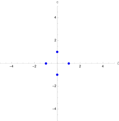
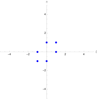
Figure 12: Real root system $\{\gamma=\xi\alpha+\eta\beta\}$ for “elliptic planes” from $|\alpha{\cdot}\beta|=0$ (left) or $1$ (right)

A more interesting case occurs for $m{=}2$. Here, the real roots lie on two straight lines (see Fig. 13 left),

$$\xi_{k}\ =\ k\qquad\Rightarrow\qquad\pm\gamma_{k}\ =\ k\,\alpha+(k{-}1)\beta\ =\ (k{-}1)\bar{\gamma}+\alpha$$ (7.22)

where $\bar{\gamma}=\alpha{+}\beta$ happens to be null and orthogonal to $\alpha$ and $\beta$. This set of roots creates the affine extension $\widehat{sl}_{2}\equiv\widehat{A}_{1}\equiv A_{1}^{(1)}$ of $sl_{2}$. Obviously, any pair of roots in this set has a scalar product of $2$ or $-2$. Such an $\widehat{sl}_{2}$ subsystem is generated by any non-orthogonal pair of real roots from levels $\ell{=}{\pm}1$ and $|\ell|{\leq}1$. Its contribution to $Y$ evaluates to

$$Y^{\Pi_{2}} \ =\ -\alpha{\wedge}\beta\,\sum_{\ell=1}^{\infty}\ell\,\bigl{\{}(s_{\alpha}s_{\beta})^{\ell}-(s_{\beta}s_{\alpha})^{\ell}\bigr{\}}\sum_{k\in\mathds{Z}}\bigl{[}k\,\bar{\gamma}{\cdot}x+\alpha{\cdot}x\bigr{]}^{-1}\bigl{[}(k{-}\ell)\,\bar{\gamma}{\cdot}x+\alpha{\cdot}x\bigr{]}^{-1}$$ (7.23)

$$\ =\ \alpha{\wedge}\beta\,\sum_{\ell=1}^{\infty}\ell\,\bigl{\{}(s_{\alpha}s_{\beta})^{\ell}-(s_{\beta}s_{\alpha})^{\ell}\bigr{\}}\,\frac{\pi}{\ell\,(\bar{\gamma}{\cdot}x)^{2}}\,\Bigl{\{}\cot\bigl{(}\pi[\ell{-}\tfrac{\alpha{\cdot}x}{\bar{\gamma}{\cdot}x}]\bigr{)}+\cot\bigl{(}\pi[\tfrac{\alpha{\cdot}x}{\bar{\gamma}{\cdot}x}]\bigr{)}\Bigr{\}}\ =\ 0$$

due to $\cot(x)+\cot(\ell\pi{-}x)=0$. Hence, also the affine subalgebras do not obstruct the commutativity of the Dunkl operators.

As soon as we go beyond level one, real root pairs with $m{>}2$ show up, and the associated quadric (7.4) is a hyperbola (see Fig. 3 right for $m{=}3$). Let us inspect the simplest such case, $m{=}3$, where the coefficient sequence happens to be the even half of the Fibonacci sequence ($k=1,2,3,\ldots$),

$$\xi_{k+1}=3\,\xi_{k}-\xi_{k-1}\quad\textrm{with}\quad\xi_{1}{=}1\quad\&\quad\xi_{0}{=}0\quad\Rightarrow\quad\xi_{k}=1,3,8,21,55,144,377,987,\ldots=f_{2k}\ ,$$ (7.24)

where $f_{n+1}=f_{n}+f_{n-1}$ with $f_{0}=0$ [22, 23]. The root scalar products take the values $\pm 2,\pm 3,\pm 7,\pm 18,\pm 47$ etc..

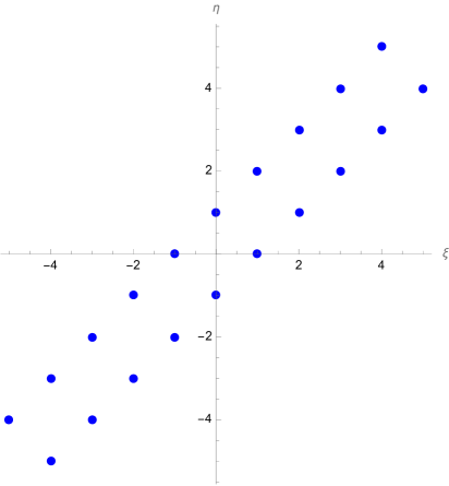
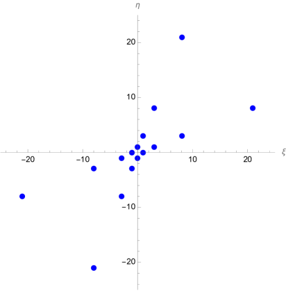
Figure 13: Real roots for a “parabolic plane” ($|\alpha{\cdot}\beta|{=}2$, left) and for a “hyperbolic plane” ($|\alpha{\cdot}\beta|{=}3$, right)

In this case, the contribution to the two-form $Y$ becomes

$$Y^{\Pi_{3}} \ =\ -\alpha{\wedge}\beta\,\sum_{\ell=1}^{\infty}\sum_{k\in\mathds{Z}}\frac{f_{2\ell}\ \bigl{\{}(s_{\alpha}s_{\beta})^{\ell}-(s_{\beta}s_{\alpha})^{\ell}\bigr{\}}}{\bigl{[}f_{2k}\,\bar{\gamma}{\cdot}x+f_{2k+1}\,\alpha{\cdot}x\bigr{]}\ \bigl{[}f_{2k-2\ell}\,\bar{\gamma}{\cdot}x+f_{2k-2\ell+1}\,\alpha{\cdot}x\bigr{]}}\ ,$$ (7.25)

with the understanding that $f_{-n}=(-1)^{n+1}f_{n}$ extends the Fibonacci sequence to the left. As numerical checks show, the individual sums over $k\in\mathds{Z}$ do not vanish, nor does the total expression. Turning off one of the two Weyl orbits in the root-sum for the Dunkl operator (6.1) does not help since odd values of $m$ require both $\alpha$ and $\beta$ to lie in ${\cal R}_{+}$, and thus only this orbit contributes here. We are forced to conclude that $Y\neq 0$ for our model, so its Dunkl operators ${\cal D}_{\mu}$ do not commute, and we cannot construct higher conserved charges unfortunately. Likewise, $Y_{\mu}^{\ \mu}$ does not vanish either, and thus $\textrm{res}\sum{\cal L}^{2}$ in (6.11) does not reproduce the Hamiltonian $H_{\Omega}$.

8 The energy spectrum

We are ultimately interested in the spectrum of our Hamiltonian $H_{\Omega}$ (1.7), which on the complex upper half-plane reads ($z=x+\mathrm{i}y$)

$$H_{\Omega}\ =\ -\tfrac{1}{2}\,y^{2}(\partial^{2}_{x}+\partial^{2}_{y})\ +\ g(g{-}1)\,U(z)\qquad\textrm{with}\quad z\in{\cal F}\ .$$ (8.1)

As a start, let us consider the situation where the coupling $g$ goes to zero (or one). Turning off the coupling does not imply removing the potential, however, since the latter is singular at $\partial{\cal F}$. Rather, it keeps an infinite wall right on the domain’s boundary, which only imposes Dirichlet boundary conditions on the free spectral problem for $\Delta$ [25].

Harmonic analysis on the fundamental domain ${\cal F}{\cup}(-\widebar{\cal F})$ of PSL(2,$\mathds{Z}$) is a rich area of mathematics intimately related to the theory of automorphic forms [26, 27, 28]. It in well known that $-\Delta$ is essentially self-adjoint and non-negative on the Hilbert space of square-integrable automorphic functions. Since it commutes with all Hecke operators $T_{n}$ and with the parity operator $P:z\mapsto-{\bar{z}}$, the spectrum on ${\cal F}{\cup}(-\widebar{\cal F})$ decomposes into

• an even part: $P$-even eigenfunctions, Neumann boundary conditions on $\partial{\cal F}$, continuous spectrum from $\tfrac{1}{4}$ to $\infty$ with embedded discrete eigenvalues, plus zero eigenvalue for the constant function,

• an odd part: $P$-odd eigenfunctions, Dirichlet boundary conditions on $\partial{\cal F}$, infinite discrete and supposedly simple spectrum above $\sim 91.14$, see Fig. 14.

Figure 14: Discrete odd eigenvalues $\lambda_{i}(0)\leq 1000$ of the Laplacian on $\textrm{PGL}(2,\mathds{Z})\backslash{\cal H}$

The $P$-even eigenfunctions are invariant under the reflections $s_{\alpha}$ while the $P$-odd ones are antiinvariant. Therefore, the extension from PSL(2,$\mathds{Z}$) to PGL(2,$\mathds{Z}$) (producing the restriction to $\cal F$) projects onto the even part. The infinite boundary walls, however, effect the opposite: they reduce the free spectrum to the odd part (for both domains), thus are responsible for removing the continuum. Hence, only the odd discrete eigenvalues are relevant for $H_{\Omega}|_{g\to 0}$, and the eigenfunctions are known as odd Maaß wave forms or cusp forms. None of the eigenvalues is known analytically, but many low-lying ones have been computed numerically to high precision [29, 30].

Even though we do not have at our disposal a closed analytic formula for our potential (notwithstanding the Poincaré series (5.19)), it is clear from the positivity of $U$ that increasing $g$ (beyond $\tfrac{1}{2}$) will raise all the discrete eigenvalues $\lambda_{i}(g)$. In case some of the integrable structure of the angular Calogero models extends to our hyperbolic one, we may expect the eigenvalue flow to be isospectral, i.e.

$$\lambda_{i}(g{+}1)=\lambda_{i+\delta(g)}(g)\qquad\textrm{thus}\qquad\lambda_{i}(g{=}n)=\lambda_{i+\delta_{n}}(0)$$ (8.2)

with some positive shifts $\delta(g)$ and $\delta_{n}$, respectively. If this holds, then the spectrum at any integer value of $g$ will agree with the odd part above except for a finite number of missing eigenvalues at the bottom. It will be interesting to test this hypothesis numerically, in order to find evidence for or against integrability of this type of models.

9 Conclusions

Spherical angular Calogero models are obtained by reducing a rational Calogero model in $\mathds{R}^{n}$ to the sphere $S^{n-1}$. Analogously, we have defined a hyperbolic angular model by reducing a Calogero Hamiltonian in $\mathds{R}^{1,n-1}$ to the (future) hyperboloid $H^{n-1}$. The main difference to the conventional angular model is the non-compactness of hyperbolic space and the replacement of a finite spherical Coxeter reflection group by an infinite hyperbolic one. As a consequence, the Calogero-type potential of the model is an infinite sum over all hyperbolic reflections and not easily obtained in a closed form. However, it is a real automorphic function of an associated hyperbolic Kac–Moody algebra.

We have worked out the details for the rank-3 case of $AE_{3}$ leading to a PGL(2,$\mathds{Z}$) invariant quantum mechanical model on the Poincaré disk or the complex upper half plane. In this case, the potential can be reformulated as a Poincaré series, which converges outside the mirror lines of PGL(2,$\mathds{Z}$). We then asked whether the integrability of the spherical angular models extends to the hyperbolic ones. To this end, we introduced the hyperbolic Dunkl operators for the $AE_{3}$ algebra and computed their commutators. It turned out that the presence of hyperbolic rank-2 subalgebras in $AE_{3}$ ruins the commutativity, which is an obstacle to integrability.

Finally, the energy spectrum of the $AE_{3}$ hyperbolic Calogero model is a deformation of the discrete parity-odd part of the spectrum of the hyperbolic Laplacian on square-integrable automorphic functions, because the singular lines of the potential impose Dirichlet boundary conditions on the boundary of the fundamental domain. It remains to be seen whether the spectral flow with the coupling $g$ is isospectral under integral increments of $g$.

Since the Weyl-alcove walls of certain hyperbolic Kac–Moody algebras are the cushions of the billard dynamics in the BKL approach [31, 32], the small-$g$ limit of our hyperbolic Kac–Moody Calogero system provides a model for cosmological billards [11]. The chaotic dynamics of such billards seems to be consistent with a formal integrability of the corresponding hyperbolic Toda-like theories [11]. Furthermore, an alternative description of BKL dynamics leads instead to Euler–Calogero–Sutherland potentials of the $\sinh^{-2}$ type, which also produce sharp walls in the BKL limit [33, 34]. This nurtures the hope that also our Calogero-type potentials retain a kind of integrability. Finally, the well-known quantum chaotic behavior of hyperbolic billards [35] may be “tamed” by turning on our Kac–Moody Calogero potential, since in the large-$g$ limit the wave function will get pinned near the bottom of the potential. We hope that this opens a door to interesting further studies in this field.

Appendix A Appendix (with Don Zagier): Computing the potential

In this appendix we investigate the numerical evaluation of the potential function $U(z)$. We have to sum over infinitely many triples $(\ell,m,n)$ or $(p,q,r)$ subject to a diophantine equation, see (5.3)–(5.5),

$$U(z)=\!\!\!\sum_{\genfrac{}{}{0.0pt}{2}{p,q,r}{p^{2}+qr=1}}\!\!\!\frac{y^{2}}{[r(x^{2}{+}y^{2})-2p\,x-q]^{2}}\ =\ \Bigl{(}\sum_{r=0}+\,2\!\sum_{r>0}\Bigr{)}\!\!\!\sum_{\genfrac{}{}{0.0pt}{2}{p,q}{p^{2}+qr=1}}\!\!\!\frac{y^{2}}{[r(x^{2}{+}y^{2})-2p\,x-q]^{2}}\,=:\,U_{0}(z)+2\,U_{>}(z)\,,$$ (A.1)

where we used that $(p,q,r)$ and $(-p,-q,-r)$ contribute equally. The $r{=}0$ part is easily summed up since then $p=\pm 1$, which yields

$$U_{0}(z)\ :=\ 2\sum_{q\in\mathds{Z}}\frac{y^{2}}{[2\,x+q]^{2}}\ =\ \frac{2\pi^{2}y^{2}}{\sin^{2}(2\pi x)}\ .$$ (A.2)

For $U_{>}$ we do not know how to compute the sum in closed form. The decomposition of the root space detailed in Section 2 suggests to slice the space of triples according to fixed values of

$$\ell=r-p-q\qquad\Rightarrow\qquad q=r-p-\ell\ ,$$ (A.3)

in which case the discussion there shows that for each fixed value of $\ell$ we are left with only a sum over finitely many pairs $(p,r)$. Specifically, if we rewrite the diophantine equation $p^{2}+qr=1$ as

$$3\,r^{2}+(r-2p)^{2}\ =\ 4(\ell\,r+1)\quad\leq\ 4\,r\,(\ell{+}1)$$ (A.4)

then we see that for $r>0$ we must have $\ell\geq 0$ and also $r\leq 4(\ell+1)/3$, reducing the sum over $r$ to a finite one. Then only those $r$ for which $4\ell\,r+4-3r^{2}$ is a square give a contribution. Thus we obtain

$$U_{>}(z)\ =\ \sum_{\ell=0}^{\infty}\sum_{r=1}^{\lfloor 4(l+1)/3\rfloor}\!\!\sum_{s^{2}=4\ell r+4-3r^{2}}\frac{y^{2}}{[r(x^{2}{+}y^{2})-(r{-}s)\,x-\frac{r+s}{2}{+}\ell]^{2}}\ ,$$ (A.5)

where the inner sum is almost always empty and never has more than two terms.

The expression (A.5) converges rather slowly. But one can do better, by going back to (A.1) and reducing the inner sum to a finite one in the following way. For each fixed $r{>}0$ we denote this inner sum by $U_{r}(z)$ and rewrite it as

$$U_{r}(z)\ =\ \frac{y^{2}}{r^{2}}\!\!\!\sum_{\genfrac{}{}{0.0pt}{2}{p\,\in\,\mathds{Z}}{p^{2}\equiv 1\,(\textrm{mod}\,r)}}\!\!\frac{1}{\bigl{[}(x-\tfrac{p}{r})^{2}+y^{2}-\tfrac{1}{r^{2}}\bigr{]}^{2}}\ =\ \frac{y^{2}}{r^{2}}\!\!\!\sum_{\genfrac{}{}{0.0pt}{2}{p\,(\textrm{mod}\,r)}{p^{2}\equiv 1\,(\textrm{mod}\,r)}}\!\!\!S\bigl{(}x-\tfrac{p}{r},\sqrt{\vphantom{|}\smash{y^{2}-\tfrac{1}{r^{2}}}}\bigr{)}$$ (A.6)

where the function $S$ is defined on $\mathds{C}{\times}\mathds{C}$  by $S(x,a):=\sum_{n\,\in\,\mathds{Z}}\bigl{[}(x-n)^{2}+a^{2}\bigr{]}^{-2}$, which obviously depends only on $x$ (mod 1). Using a partial fraction decomposition of the summand together with Euler’s formulæ for $\sum_{n\in\mathds{Z}}1/(x{+}n)$ and $\sum_{n\in\mathds{Z}}1/(x{+}n)^{2}$, we find the closed formula

$$S(x,a)\ =\ \frac{\pi}{2\,a^{3}}\,\frac{\sinh(2\pi\,a)}{\cosh(2\pi\,a)-\cos(2\pi\,x)\vphantom{\big{|}^{2}}}\ +\ \frac{\pi^{2}}{a^{2}}\,\frac{\cosh(2\pi\,a)\,\cos(2\pi\,x)-1}{\bigl{(}\cosh(2\pi\,a)-\cos(2\pi\,x)\bigr{)}^{2}}\ .$$ (A.7)

Inserting this into (A.6) then expresses each $U_{r}(z)$ as a finite sum of elementary functions, and formula (A.1) takes on the more explicit form

$$U(z)\ =\ \frac{2\pi^{2}\,y^{2}}{\sin^{2}(2\pi x)}\ +\ 2\,\sum_{r=1}^{\infty}\ \frac{y^{2}}{r^{2}}\!\!\!\sum_{\genfrac{}{}{0.0pt}{2}{p\,(\textrm{mod}\,r)}{p^{2}\equiv 1\,(\textrm{mod}\,r)}}\!\!\!S\bigl{(}x-\tfrac{p}{r},\sqrt{\vphantom{|}\smash{y^{2}-\tfrac{1}{r^{2}}}}\bigr{)}$$ (A.8)

in which we now simply define $S(x,a)$ by the trigonometric formula (A.7).

Formula (A.8) is both simpler and more rapidly convergent than the original expression (A.1), since the internal infinite sums have been evaluated explicitly, and it also converges more rapidly than the “slicing by $\ell\,$” formula (A.5). As a demonstration, we list in the table below ten-digit values of the partial sums $U(z,R)$ defined by truncating (A.8) at $r{=}R$ for a typical point $z_{1}=0.1+0.7\,\mathrm{i}$ and values of $R$ going up to one million. We have also included the values $U(z_{2},R)$ at the modular image $z_{2}=-1/z_{1}=-0.2+1.4\,\mathrm{i}$, both as a test of the modularity of $U(z)$ and as a confirmation of the accuracy of the computation.

$R$	$10\,000$	$20\,000$	$50\,000$	$100\,000$	$200\,000$	$500\,000$	$1\,000\,000$
$\!\!U(z_{1},R)\!\!\phantom{\Big{|}}$	52.24167922 ​​	​​52.24327256 ​​	​​52.24429208 ​​	​​52.24465475 ​​	​​52.24484553 ​​	​​52.24496635 ​​	​​52.24500890 ​​
$\!\!U(z_{2},R)\!\!$	52.24339662 ​​	​​52.24417862 ​​	​​52.24467954 ​​	​​52.24485793 ​​	​​52.24495185 ​​	​​52.24501138 ​​	​​52.24503236 ​​

It takes PARI about 17 minutes for $R{=}10^{5}$ and about 28 hours for $R{=}10^{6}$ on a standard workstation to compute the values for each point $z_{i}$ given in this table. The output suggests that the final numbers are correct to about 7 significant digits.

The very erratic dependence of the numbers $U_{r}(z)$ on $r$, due to the sum over square-roots of $1$ modulo $r$ in (A.6), prohibits further analytic simplification. For the same reason, the infinite sum for $U(z)$, although convergent, is not very tractable numerically. However, the convergence of the partial sums $U(z,R)$ for $R\to\infty$ can be accelerated by adding a suitable correction term. The following heuristic argument suggests what this correction term should be. If the inner sum in (A.8) were over all values of $p$ (mod $r$) then, since the value of $\sqrt{\vphantom{|}\smash{y^{2}-\tfrac{1}{r^{2}}}}\approx y$ is close to $y$ for $r$ large, this inner sum for large $r$ would simply be $r$ times a Riemann sum for the integral $\int_{\mathds{R}/\mathds{Z}}S(x,y)\,\mathrm{d}x=\int_{\mathds{R}}(x^{2}{+}y^{2})^{-2}\mathrm{d}y=\pi/2y^{3}$ and hence could be approximated by $r\pi/2y^{3}$. The actual inner sum is only over $N(r)$ rather than $r$ values of $p$ (mod $r$), where $N(r)$ denotes the number of square-roots of $1$ modulo $r$. Hence, if these square-roots are more or less uniformly distributed on the interval $[1,r]$ on the average, which is a reasonable heuristic assumption, then the value of the inner sum should be roughly $N(r)\,\pi/y^{3}$ on average. Therefore, the contribution of the terms in (A.8) with $r{>}R$ (the “tail”) should be approximately $\pi/y$ times $\sum_{r>R}N(r)/r^{2}$ for $R$ large. The value of the arithmetic function $N(r)$ fluctuates a lot, but its average behavior is quite regular, and one can give the asymptotic value of the sum $\sum_{r>R}N(r)/r^{2}$ without difficulty. Specifically, from the Chinese remainder theorem we find that $N(r)$ is multiplicative, meaning that $N\bigl{(}\prod p_{i}^{\nu_{i}}\bigr{)}=\prod N(p_{i}^{\nu_{i}})$, and $N(p^{\nu})$ in turn is easily evaluated as 2 for $p$ an odd prime and $\nu{\geq}1$ (the only two square-roots of 1 in this case being $\pm 1$ (mod $p^{r}$)), and as 1 or 2 or 4 for $p{=}2$ and $\nu{=}1$, $2$, or ${\geq}3$, respectively (the only square-roots of 1 in the latter case being $\pm 1$ and $\pm 1{+}2^{r-1}$ (mod $2^{r}$)). This gives

$${\cal N}(s) :=\ \sum_{r=1}^{\infty}\frac{N(r)}{r^{s}}\ =\ \Bigl{(}1+\frac{1}{2^{s}}+\frac{2}{4^{s}}+\frac{4}{8^{s}}+\frac{4}{16^{s}}+\ldots\Bigr{)}\,\prod_{p>2}\Bigl{(}1+\frac{2}{p^{s}}+\frac{2}{p^{2s}}+\frac{2}{p^{3s}}+\ldots\Bigr{)}$$ (A.9)

$$\ =\ \frac{1\,+\,2^{-2s}+2^{1-3s}}{1\,-\,2^{-s}}\,\prod_{p>2}\frac{1+p^{-s}}{1-p^{-s}}\ =\ \bigl{(}1\,-\,2^{-s}+2^{1-2s}\bigr{)}\,\frac{\zeta(s)^{2}}{\zeta(2s)}\ ,$$

where $\zeta(s)$ denotes the Riemann zeta function. In particular, $\mathcal{N}(s)$ has a double pole at $s{=}1$ with principal part $\frac{\zeta(2)^{-1}}{(s-1)^{2}}\,+\,\text{O}\bigl{(}\frac{1}{s-1}\bigr{)}$, so $N(r)$ behaves “on the average” like $\zeta(2)^{-1}\log r$, and $\sum\limits_{r>R}\frac{N(r)}{r^{2}}$ is asymptotically equal to $\zeta(2)^{-1}\,\frac{\log R}{R}$. This suggests that we can improve the convergence of $\sum U_{r}(z)$ by replacing the partial sums $U(z,R)$ by

$$U^{(0)}(z,R)\ =\ U(z,R)\ +\ \frac{6}{\pi y}\,\frac{\log R}{R}\ .$$ (A.10)

This is indeed the case, as we see from the following table below, in which we have tabulated the corrected partial sums with the same parameters as before.

$R$	$10\,000$	$20\,000$	$50\,000$	$100\,000$	$200\,000$	$500\,000$	$1\,000\,000$ ​​
$\!\!U^{(0)}(z_{1},R)\!\!\phantom{\Big{|}}$	52.24419214 ​​	​​52.24462358 ​​	​​52.24488249 ​​	​​52.24496886 ​​	​​52.24501205 ​​	​​52.24503796 ​​	​​52.24504659 ​​
$\!\!U^{(0)}(z_{2},R)\!\!$	52.24465308 ​​	​​52.24485413 ​​	​​52.24497474 ​​	​​52.24501499 ​​	​​52.24503511 ​​	​​52.24504718 ​​	​​52.24505121

We can improve these values further by adding an appropriate term $C/R$ to (A.10), where $C$ is a constant depending on $z$ but not on $R$. For this, we must first give a more precise estimate of $\sum_{r>R}N(r)/r^{2}$ for $R$ large. The function $\zeta(s)$ is holomorphic except for a simple pole at $s{=}1$, with $\zeta(1{+}\varepsilon)=\varepsilon^{-1}+\gamma+\textrm{O}(\varepsilon)$ as $\varepsilon\to 0$, where $\gamma$ is Euler’s constant. It has no zeros in the half-plane $\Re(s)>1$ (or even $\Re(s)>\frac{1}{2}$ if we assume the Riemann Hypothesis), so $\mathcal{N}(s)$ has the same poles as $-c\;\zeta^{\prime}(s)+c_{1}\,\zeta(s)$ in the half-plane $\Re(s)>\frac{1}{2}$ (resp. $>\frac{1}{4}$ on RH), where

$$c\ =\ \frac{1}{\zeta(2)}\ =\ \frac{6}{\pi^{2}}\ =\ 0.6079271\dots\quad\text{and}\quad c_{1}\ =\ c\,\Bigl{(}2\gamma\,-\frac{1}{2}\,\log 2\,-\,2\,\frac{\zeta^{\prime}(2)}{\zeta(2)}\Bigr{)}\ =\ 1.184108\cdots\ .$$ (A.11)

This implies that $N(r)$ behaves on the average like $c\,\log\,r+c_{1}$, and that we have the asymptotic estimate

$$\sum_{r=R+1}^{\infty}\frac{N(r)}{r^{2}}\ \sim\ \frac{c\,\log R+c+c_{1}}{R}\ ,$$ (A.12)

with an error of the order of $R^{-3/2+\varepsilon}$ unconditionally or $R^{-7/4+\varepsilon}$ if we assume the Riemann Hypothesis. This suggests that we can further improve the convergence of $\sum U_{r}(z)$ by replacing $U^{(0)}(z,R)$ of (A.10) with

$$U^{(1)}(z,R)\ =\ U^{(0)}(z,R)\ +\ \frac{\pi}{y}\,\frac{c+c_{1}}{R}\ ,$$ (A.13)

and this is indeed confirmed by the values shown in the following table.

$R$	$10\,000$	$20\,000$	$50\,000$	$100\,000$	$200\,000$	$500\,000$	$1\,000\,000$ ​​
$\!\!U^{(1)}(z_{1},R)\!\!\phantom{\Big{|}}$	52.24499640 ​​	​​52.24502571 ​​	​​52.24504334 ​​	​​52.24504929 ​​	​​52.24505226 ​​	​​52.24505404 ​​	​​52.24505464 ​​
$\!\!U^{(1)}(z_{2},R)\!\!$	52.24505521 ​​	​​52.24505520 ​​	​​52.24505517 ​​	​​52.24505520 ​​	​​52.24505522 ​​	​​52.24505522 ​​	​​52.24505523

However, although these values are better, we see clearly from the graphs shown in Figure 15 that even $U^{(1)}(z_{1},R)$, though much more nearly constant than $U^{(0)}(z_{1},R)$, is still off by a linear term in $1/R$.

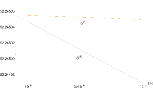
Figure 15:

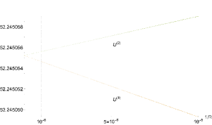
Figure 16:

To understand the reason for this, we must refine the heuristic argument given above. We begin by noting that the values of $\frac{p}{r}$ for $p^{2}\equiv 1$ (mod $r$) are in fact not completely uniformly distributed modulo 1, even on the average, because the two values corresponding to $p\equiv\pm 1$ (mod $r$) are always very near to 0. For the remaining $N(r){-}2$ values the heuristic assumption of equidistribution at first sight still seems plausible, in which case the corresponding contribution to each term $U_{r}(z)$ with $r$ large would have the same average behavior as $\bigl{(}N(r){-}2\bigr{)}\frac{\pi}{r^{2}y}$, but the two values of $p/r$ near 0 give a contribution to $U_{r}(z)$ of approximately $2y^{2}S(x,y)/r^{2}$ each. This suggests the improved correction

$$U^{(2)}(z,R)\ =\ U^{(1)}(z,R)\ +\ \frac{4y^{2}S^{*}(x,y)}{R}\qquad\text{with}\qquad S^{*}(x,y):=S(x,y)-\frac{\pi}{2y^{3}}$$ (A.14)

instead of (A.13), and this indeed does give a further improvement of the convergence, as one sees in the table below and also in the graph in Figure 16. But this same graph makes it clear that we still do not have the right linear correction term. The reason for this is more subtle and is the most interesting part of the discussion.

$R$	$10\,000$	$20\,000$	$50\,000$	$100\,000$	$200\,000$	$500\,000$	$1\,000\,000$
$\!\!U^{(2)}(z_{1},R)\!\!\phantom{\Big{|}}$	52.24509364 ​​	​​52.24507433 ​​	​​52.24506279 ​​	​​52.24505901 ​​	​​52.24505712 ​​	​​52.24505599 ​​	​​52.24505561 ​​
$\!\!U^{(2)}(z_{2},R)\!\!$	52.24505562 ​​	​​52.24505540 ​​	​​52.24505525 ​​	​​52.24505524 ​​	​​52.24505524 ​​	​​52.24505523 ​​	​​52.24505523 ​​

This final heuristic argument depends on the observation that not only are the two obvious square-roots $\pm 1$ of 1 (mod $r$) not randomly distributed modulo $r$, but that there are infinitely many other non-randomly distributed square-roots, each occurring for a set of integers $r$ of positive asymptotic density. For instance, if $r\!\equiv 10\!\pmod{25}$, which happens for $4\%$ of all integers, then the two further numbers $\pm{(r/5\,-\,1)}$ are also square-roots of 1 (mod $r$), because $r/5\,-\,1$ is congruent to $-1$ modulo $r/5$ and to $+1$ modulo 5. For these two values of $p$, one has $\frac{p}{r}\equiv\pm\frac{1}{5}+\text{O}\bigl{(}\frac{1}{r}\bigr{)}$, which are indeed not randomly distributed. More generally, for any rational number $\alpha=N/D$ with $N$ and $D$ coprime and $D>0$, we consider integers $r{>}0$ of the form $D\,n$ with $n\equiv-2N^{-1}\!\pmod{D}$. Then the number $p=Nn+1$ is congruent to 1 modulo $n$ and to $-1$ modulo $D$, so that $p^{2}\equiv 1\!\!\pmod{r}$, while $\frac{p}{r}=\frac{N}{D}+\frac{1}{r}$ is extremely close to $\alpha$ if $r$ is large. For fixed $\alpha$, the set of integers $r$ of this form constitutes a single congruence class modulo $D^{2}$ and hence has asymptotic density $1/D^{2}$. Hence, approximating $x-\frac{p}{r}$ by $x-\alpha$ and $\sqrt{\vphantom{|}\smash{y^{2}-\tfrac{1}{r^{2}}}}$ by $y$ in (A.6) , we see that the total contribution of these terms to the “tail” $r>R$ in (A.6) is approximately $\frac{2\,y^{2}}{D^{2}R}\,S(x-\alpha,y)$. To get the final answer, we must sum this over all rational numbers $\alpha\!\pmod{1}$, i.e., over all denominators $D>0$ and all numerators $N\!\pmod{D}$ prime to $N$.

The easiest way to do this is to use the Fourier expansion of the periodic function $S(x,a)$ which is given by

$$S(x,a)\ =\ \frac{\pi}{a^{3}}\,\Bigl{(}\frac{1}{2}\,+\,\sum_{n=1}^{\infty}\bigl{(}1+2\pi na\bigr{)}\,\mathrm{e}^{-2\pi na}\,\cos(2\pi nx)\Bigr{)}\ .$$ (A.15)

(There are two ways to see this: either one writes the Fourier expansion of $S(x,a)$ as $\sum_{n\in\mathds{Z}}S_{n}(a)\,\mathrm{e}^{2\pi inx}$ with $S_{n}(a)=\int_{\mathds{R}/\mathds{Z}}S(x,a)\,\mathrm{e}^{-2\pi nx}\,\mathrm{d}x=\int_{\mathds{R}}\frac{\mathrm{e}^{-2\pi nx}}{(x^{2}+a^{2})^{2}}\,\mathrm{d}x$ and computes the integral by the Cauchy residue theorem, or else one simply evaluates the expression on the right-hand side of (A.15) in closed form using the formulæ for the sum of a geometric series or its derivative, obtaining precisely the right-hand side of (A.7).) The constant term $\pi/2a^{3}$, in this expansion, with $a$ replaced by $\sqrt{\vphantom{|}\smash{y^{2}-\tfrac{1}{r^{2}}}}\approx y$ and inserted into (A.8), gives exactly the approximation $\frac{\pi}{y}\,\sum_{r>R}\frac{N(r)}{r^{2}}$ to $U(z)-U(z,R)$ that we used in our initial heuristic argument and that led via (A.12) to the function $U^{(1)}(z,R)$ defined in (A.13). The further correction term coming from all rational numbers $\alpha\!\pmod{1}$ as explained above therefore has the form $C(z)/R$, with $C(z)$ given by

$$C(x{+}\mathrm{i}y)\ =\ 2y^{2}\,\sum_{D=1}^{\infty}\frac{1}{D^{2}}\!\!\sum_{\genfrac{}{}{0.0pt}{2}{N\,\text{(mod\leavevmode\nobreak\ $D$)}}{(N,D)=1}}\!\!S^{*}\bigl{(}x{-}\tfrac{N}{D},y\bigr{)}$$ (A.16)

with $S^{*}(x,a)$ as in (A.14). Replacing $S^{*}(x,a)$ by its expression as a sum of exponentially small terms given in (A.15) and interchanging the order of summation, we find

$$C(x{+}\mathrm{i}y)\,=\,\frac{2\pi}{y}\sum_{n=1}^{\infty}\varepsilon(n)\,(1{+}2\pi ny)\,\mathrm{e}^{-2\pi ny}\,\cos(2\pi nx)\qquad\text{with}\qquad\varepsilon(n):=\sum_{D=1}^{\infty}\frac{1}{D^{2}}\!\!\sum_{\genfrac{}{}{0.0pt}{2}{N\,\text{(mod\leavevmode\nobreak\ $D$)}}{(N,D)=1}}\!\!\mathrm{e}^{2\pi\mathrm{i}nN/D}\ .$$ (A.17)

The sum over $N\!\pmod{D}$ is the well-known Ramanujan sum, whose value is given as the sum of $d\,\mu(D/d)$ ($\mu=$ Möbius function) over all common divisors $d$ of $D$ and $n$. Therefore, writing $D$ as $d\,k$ with $k>0$ we find

$$\varepsilon(n)\ =\ \sum_{d|n}\sum_{k=1}^{\infty}\frac{\mu(k)}{d\,k^{2}}\ =\ \frac{6}{\pi^{2}}\;\sigma_{-1}(n)\ ,$$ (A.18)

where $\sigma_{i}(n):=\sum_{d|n}d^{i}$ as usual. This finally gives ($z=x{+}\mathrm{i}y$)

$$C(z)\ =\ \frac{12}{\pi y}\,\sum_{n=1}^{\infty}\bigl{(}\sigma_{-1}(n)\,+\,2\pi\,\sigma_{1}(n)\,y\bigr{)}\,\mathrm{e}^{-2\pi ny}\,\cos(2\pi nx)\ =\ -\frac{12}{\pi y}\,\log\bigl{|}\eta(z)\bigr{|}\,-\,\Re\bigl{(}E_{2}(z)\bigr{)}\ ,$$ (A.19)

where $\eta(z)=\mathrm{e}^{\pi\mathrm{i}z/12}\prod(1-\mathrm{e}^{2\pi\mathrm{i}nz})^{24}$ and $E_{2}(z)=1-24\sum\sigma_{1}(n)\,\mathrm{e}^{2\pi\mathrm{i}nz}$ denote the Dedekind eta-function and the quasimodular Eisenstein series of weight 2 on the full modular group, respectively. Note that each of the two terms on the right-hand side of (A.19) is the sum of a constant $\pm 1$ and an exponentially small term of the order of $\mathrm{e}^{-2\pi y}$, but that their sum $C(z)$ decays exponentially as $y{=}\Im(z)$ grows. This explains why in the tables above the convergence of both $U^{(1)}$ and $U^{(2)}$ was much faster for $z_{2}$ ($y_{2}{=}1.4$) than for $z_{1}$ ($y_{1}{=}0.7$).

Summarizing, we have given an argument suggesting that the “correct” refinement of the truncated sum $U(z,R)$ should be given by

$$U^{(\infty)}(z,R)\ =\ U^{(1)}(z,R)\ +\ \frac{C(z)}{R}$$ (A.20)

with $C(z)$ defined by (A.19) for $z$ in the complex upper half-plane. The table below and the graph in Figure 17 both confirm that this improved version of the previous functions $U^{(i)}(z,R)$ ($i=0,1,2$) does indeed converge very much faster to its limiting value $U(z)$ than any of them did, with the error now decaying faster than $1/R$. (Both the numerical experiments and a heuristic argument suggest that the true order of magnitude of this difference should be something more like $(\log R)^{2}/R^{2}$.) Finally, the graph in Figure 18 gives one last improvement. Here, we have replaced the function $U^{(\infty)}(z,R)$ by a function $\overline{U}(z,R)$ defined as the average value of the numbers $U^{(\infty)}(z,R^{\prime})$ for $R^{\prime}$ in the (somewhat arbitrarily chosen) interval $[2R/3,R]$. The calculations up to the same limit $R{=}10^{6}$ as before now yield at least 12 significant digits rather than the original 7.

$R$	$10\,000$	$50\,000$	$100\,000$	$500\,000$	$1\,000\,000$
$\!\!U^{(\infty)}(z_{1},R)\!\!\phantom{\Big{|}}$	52.2450557618857 ​​	​​52.2450552157850 ​​	​​52.2450552237500 ​​	​​52.2450552285072 ​​	​​52.2450552288639 ​​
$\!\!U^{(\infty)}(z_{2},R)\!\!$	52.2450554614623 ​​	​​52.2450552195214 ​​	​​52.2450552255882 ​​	​​52.2450552288339 ​​	​​52.2450552288596 ​​

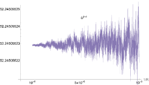
Figure 17:

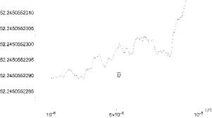
Figure 18:

For the sake of honesty it should perhaps be mentioned that, if our goal were simply to obtain a better convergence of $U(z,R)$ to $U(z)$ as $R\to\infty$, then we could have avoided the whole discussion of the “right” linear correction term $C/R$ to (A.10). One can simply use a least-squares fit to obtain $C$ numerically from our tabulated values (as we in fact did originally, with results that were not all that much worse than $U^{(\infty)}$). Alternatively, at the cost of a little loss of accuracy, one can replace $U^{(0)}(R)$ by the expression $2\,U^{(0)}(R)-U^{(0)}(R/2)$, which eliminates any linear term in $1/R$ and is unchanged by employing $U^{(1)}$, $U^{(2)}$, or $U^{(\infty)}$ instead of $U^{(0)}$. However, our analysis leading to the final correction term as given by (A.10), (A.13) and (A.20) with (A.19) is mathematically interesting and seemed worth giving, especially in view of the unexpected occurrence of the nearly modular functions $\log\bigl{|}\eta(z)\bigr{|}$ and $\Re\bigl{(}E_{2}(z)\bigr{)}$.

Acknowledgments

I am grateful to Don Zagier for illuminating discussions and to Hermann Karcher for helpful comments. I also thank Luca Romano for collaboration at an early stage of this project and Axel Kleinschmidt for pointing out some literature.

References

[1]
F. Calogero,
Solution of the one-dimensional N-body problem with quadratic
and/or inversely quadratic pair potentials,
J. Math. Phys. 12 (1971) 419–436;
Erratum, ibidem37 (1996) 3646.
[2]
M.A. Olshanetsky, A.M. Perelomov,
Classical integrable finite-dimensional systems related to Lie algebras,
Phys. Rept. 71 (1981) 313–400.
[3]
M.A. Olshanetsky, A.M. Perelomov,
Quantum integrable systems related to Lie algebras,
Phys. Rept. 94 (1983) 313–404.
[4]
M.V. Feigin,
Intertwining relations for spherical parts of generalized Calogero operators,
Theor. Math. Phys. 135 (2003) 497–509.
[5]
T. Hakobyan, A. Nersessian, V. Yeghikyan,
The cuboctahedric Higgs oscillator from the rational Calogero model,
J. Phys. A: Math. Theor. 42 (2009) 205206
[arXiv:0808.0430 [hep-th]].
[6]
M.V. Feigin, O. Lechtenfeld and A. Polychronakos,
The quantum angular Calogero–Moser model,
JHEP 07 (2013) 162
[arXiv:1305.5841 [math-ph]].
[7]
A.P. Polychronakos,
Physics and Mathematics of Calogero particles,
J. Phys. A: Math. Gen. 39 (2006) 12793
[arXiv:hep-th/0607033].
[9]
B. Sutherland,
Exact results for a quantum many-body problem in one dimension. I & II,
Phys. Rev. A 4 (1971) 2019–2021 (1971); ibid. A 5 (1972) 1372–1376.
[10]
M.W. Davis,
The Geometry and Topology of Coxeter Groups,
London Mathematical Society Monographs Series vol. 32,
Princeton University Press, 2008.
[11]
T. Damour, M. Henneaux and H. Nicolai,
Cosmological billards,
Class. Quant. Grav. 20 (2003) R145–R200
[arXiv:hep-th/0212256].
[12]
A.J. Feingold and I.B. Frenkel,
A hyperbolic Kac–Moody algebra and the theory of Siegel modular forms of genus 2,
Math. Ann. 263 (1983) 87–144.
[14]
S.-J. Kang,
Root multiplicities of the hyperbolic Kac–Moody algebra ,
J. Algebra 160 (1993) 492–523.
[15]
S.-J. Kang,
On the hyperbolic Kac–Moody Lie algebra ,
Trans. Amer. Math. Soc. 341 (1994) 623–638.
[16]
T. Damour, M. Henneaux, B. Julia and H. Nicolai,
Hyperbolic Kac–Moody algebras and chaos in Kaluza–Klein models,
Phys. Lett. B 509 (2001) 323
[arXiv:hep-th/0103094].
[17]
L. Carbone, A. Conway, W. Freyn and D. Penta,
Weyl group orbits on Kac–Moody root systems,
J. Phys. A: Math. Theor. 47 (2014) 445201
[arXiv:1407.3375 [math.GR]].
[18]
D. Zagier,
Eisenstein series and the Riemann zeta function,
in: Automorphic Forms, Representation Theory and Arithmetic,
pp. 275–301, Springer 1981.
[20]
M. Feigin and T. Hakobyan,
On the algebra of Dunkl angular momentum operators,
JHEP 11 (2015) 107
[arXiv:1409.2480 [math-ph]].
[21]
A.J. Feingold and H. Nicolai,
Subalgebras of hyperbolic Kac–Moody algebras,
Contemp. Math. 343, Amer. Math. Soc. (2004) 97–114.
[22]
A.J. Feingold,
A hyperbolic GCM Lie algebra and the Fibonacci numbers,
Proc. Amer. Math. Soc. 80 (1980) 379–385.
[23]
D.A. Penta,
Decomposition of the rank 3 Kac–Moody Lie algebra with respect to
the rank 2 hyperbolic subalgebra ,
PhD dissertation, Binghampton University, SUNY
[arXiv:1605.06901 [math.RA]].
[24]
G.J. Heckman,
A remark on the Dunkl differential-difference operators,
in: W. Barker, P. Sally (eds.), Harmonic analysis on reductive groups,
Progr. Math. 101 (1991) 181–191.
[25]
A. Kleinschmidt, M. Koehn and H. Nicolai,
Supersymmetric quantum cosmological billiards,
Phys. Rev. D 80 (2009) 061701
[arXiv:0907.3048 [gr-qc]].
[26]
M. Eie and A. Krieg,
The Maaß space on the half-plane of Cayley numbers of degree two,
Math. Z. 210 (1992) 113–128.
[27]
H. Iwaniec,
Spectral methods of automorphic forms,
Am. Math. Soc. Graduate Studies in Mathematics vol. 53 (2002).
[28]
D. Chatzakos,
Spectral theory of automorphic forms and related problems,
lecture notes, 2020,
dimitrioschatzakos.com/wp-content/uploads/2020/02/Notes-for-the-course.pdf.
[29]
G. Steil,
Eigenvalues of the Laplacian and of the Hecke operators for PSL(2,),
DESY preprint 94-028 (March 1994).
[30]
H. Then,
Maaß cusp forms for large eigenvalues,
Math. Comp. 74 (2004) 363
[arXiv:math-ph/0305047].
[31]
V.A. Belinskii, I.M. Khalatnikov and E.M. Lifshitz,
Oscillatory approach to a singular point in the relativistic cosmology,
Adv. Phys. 19 (1970) 525.
[32]
V.A. Belinskii, I.M. Khalatnikov and E.M. Lifshitz,
A general solution of the Einstein equations with a time singularity,
Adv. Phys. 31 (1982) 639.
[33]
M.P. Ryan,
The oscillatory regime near the singularity in Bianchi-type IX universes,
Ann. Phys. (N.Y.) 70 (1972) 301.
[34]
A.M. Khvedelidze and D.M. Mladenov,
Bianchi I cosmology and Euler–Calogero–Sutherland model,
Phys. Rev. D 66 (2002) 123504
[arXiv:gr-qc/0208037].
[35]
E. Bogomolny,
Quantum and arithmetical chaos,
lecture notes
[arXiv:nlin/0312061].