Sparsity and Heterogeneous Dropout for Continual Learning in the Null Space of Neural Activations

Abstract

Continual/lifelong learning from a non-stationary input data stream is a cornerstone of intelligence. Despite their phenomenal performance in a wide variety of applications, deep neural networks are prone to forgetting their previously learned information upon learning new ones. This phenomenon is called “catastrophic forgetting” and is deeply rooted in the stability-plasticity dilemma. Overcoming catastrophic forgetting in deep neural networks has become an active field of research in recent years. In particular, gradient projection-based methods have recently shown exceptional performance at overcoming catastrophic forgetting. This paper proposes two biologically-inspired mechanisms based on sparsity and heterogeneous dropout that significantly increase a continual learner’s performance over a long sequence of tasks. Our proposed approach builds on the Gradient Projection Memory (GPM) framework. We leverage k-winner activations in each layer of a neural network to enforce layer-wise sparse activations for each task, together with a between-task heterogeneous dropout that encourages the network to use non-overlapping activation patterns between different tasks. In addition, we introduce two new benchmarks for continual learning under distributional shift, namely Continual Swiss Roll and ImageNet SuperDog-40. Lastly, we provide an in-depth analysis of our proposed method and demonstrate a significant performance boost on various benchmark continual learning problems.

1 Introduction

The capability to continually acquire and update representations from a non-stationary environment, referred to as continual/lifelong learning, is one of the main characteristics of intelligent biological systems. The embodiment of this capability in machines, and in particular in deep neural networks, has attracted much interests from the artificial intelligence (AI) and machine learning (ML) communities (Farquhar & Gal, 2018; von Oswald et al., 2019; Parisi et al., 2019; Mundt et al., 2020; Delange et al., 2021). Continual learning is a multi-faceted problem, and a continual/lifelong learner must be capable of: 1) acquiring new skills without compromising old ones, 2) rapid adaptation to changes, 3) applying previously learned knowledge to new tasks (forward transfer), and 4) applying newly learned knowledge to improve performance on old tasks (backward transfer), while conserving limited resources. Vanilla deep neural networks (DNNs) are particularly bad lifelong learners. DNNs are prone to forgetting their previously learned information upon learning new ones. This phenomenon is referred to as “catastrophic forgetting” and is deeply rooted in the stability-plasticity dilemma. A large body of recent work focuses on overcoming catastrophic forgetting in DNNs.

The existing approaches for overcoming catastrophic forgetting can be broadly organized into memory-based methods (including memory rehearsal/replay, generative replay, and gradient projection approaches) (Shin et al., 2017; Farquhar & Gal, 2018; Rolnick et al., 2019; Rostami et al., 2020; Farajtabar et al., 2020), regularization-based approaches that penalize changes to parameters important to past tasks (Kirkpatrick et al., 2017; Zenke et al., 2017; Aljundi et al., 2018a; Kolouri et al., 2020; li2, 2021; von Oswald et al., 2019), and 3) architectural methods that rely on model expansion, parameter isolation, and masking (Schwarz et al., 2018; Mallya & Lazebnik, 2018; Mallya et al., 2018; Wortsman et al., 2020). Many recent and emerging approaches leverage a combination of the above mentioned mechanisms, e.g., (Van de Ven & Tolias, 2019). Among the mentioned approaches, gradient-projection based methods (Farajtabar et al., 2020; Saha et al., 2020; Deng et al., 2021; Wang et al., 2021; Lin et al., 2022) have recently shown exceptional performance at overcoming catastrophic forgetting. In this paper, we will focus on the Gradient Projection Memory (GPM) approach introduced by Saha et al. (2020), and propose two biologically-inspired improvements for GPMs, which are algorithmically simple yet they lead to a significant improvement in performance of the GPM algorithm.

Sparsity is a critical concept that commonly occurs in biological neural networks. Sparsity in biological systems emerges as a mechanism for conserving energy and avoiding neural activations’ cost to an extent that is possible. Neuroscientists estimate only 5-10% of the neurons in a mammalian brain to be active concurrently (Lennie, 2003), leading to sparse decorrelated patterns of neural activations in the brain (Yu et al., 2014). Similarly in ML, sparsity plays a critical role for obtaining models that are more generalizable Makhzani & Frey (2013) and are robust to noisy inputs and adversarial attacks Guo et al. (2018). Moreover, sparse neural networks are critical in deploying power-efficient ML models. In continual learning, various recent studies show the role of sparsity in neural parameters (Schwarz et al., 2021) or in neural activations (i.e., representations) (Aljundi et al., 2018b; Jung et al., 2020; Gong et al., 2022) in overcoming catastrophic forgetting. The existing work combine sparse model with regularization based continual learning or memory replay approaches and show significant improvements over baseline performances. These methods enforce sparsity via inhibition of activations (Aljundi et al., 2018b; Ahmad & Scheinkman, 2019), through regularization (Jung et al., 2020), or by optimization reparameterization during training (Schwarz et al., 2021). In this paper, we consider continual learning under power constraints and study the role of sparsity for continual learning in the nullspace of neural activations. We propose an adaptation of the k-winner algorithm (Ahmad & Scheinkman, 2019), to enforce sparsity and encourage decorrelated neural activations among tasks. The power consumption of our proposed algorithm at the inference is significantly smaller than that of the GPM, while it provides a demonstrable advantage over GPM in learning a large sequence of tasks.

Contributions. Our main contributions in this paper are: 1) proposing a modification of the k-winner algorithm that leads to a significant gain in continual learning from long sequences of tasks, 2) showing that sparse activations through the modified k-winner algorithm result in low-rank neural activation subspaces at different layers of a neural network, 3) introducing conditional dropout as a mechanism to encourage decorrelated activations between different tasks, 4) introducing Continual Swiss Roll as a lightweight and interpretable, yet challenging, synthetic benchmark for continual learning, and 5) introducing the ImageNet SuperDog-40 as a ‘distributional shift’ benchmark for continual learning. We demonstrate the effectiveness of our proposed method on various benchmark continual learning tasks and compare with existing approaches.

2 Related Work

Gradient-projection based approaches. These methods rely on the observation that during learning a new task the Stochastic Gradient Descent (SGD)- or its variants- is oblivious to the past knowledge Farajtabar et al. (2020). Hence, generally speaking, these methods rely on carrying the gradient information from previous tasks, whether by storing samples from old tasks or by learning gradient subspaces, and adjust the gradient for the current task such that it does not unlearn or interfere with previous tasks. In Orthogonal Gradient Descent (OGD), Farajtabar et al. (2020) store a memory of the loss gradients on previous tasks and project the loss gradient for the current task onto the nullspace of the previous gradients in the memory. This method requires a growing memory in the number of tasks. This idea is extended in Saha et al. (2020) and Wang et al. (2021) take this idea one step further and propose to carry and update a gradient subspace for previous tasks, and project the current loss gradient onto the nullspace of previous gradients, requiring a fix-size memory. This core idea has been extended in numerous directions in recent publications, e.g., Deng et al. (2021). One major shortcoming of the gradient projection approaches, however, is that, by design, these methods provide no backward transfer. This shortcoming has led to more recent studies (Lin et al., 2022), that relax the orthogonal projection and allow for gradients to live in the subspace of ‘similar’ previous tasks leading to some backward transfer among tasks.

Neural networks with low-rank activation subspaces. low-rank structure of neural activations (i.e., low-rank representations) is a relatively understudied research area. The existing work, for instance, show that inducing low-rank structure on neural activations could result in networks that are more robust to adversarial attacks, and are also, not surprisingly, more compressible Sanyal et al. (2019). As another example, Chen et al. (2018) show the effectiveness of a low-rank constraint on the embedding space of an autoencoder in clustering applications. More relevant to our work, is the fantastic work by Chaudhry et al. (2020), in which the authors learn tasks in orthogonal low-rank vector subspaces (layer-wise) to minimize interference between tasks. We approach the problem from a different angle. Our rationale is that having a lower rank subspace for neural activations of previous tasks, would lead to a larger nullspace for projecting the loss gradient of the current task. In other words, enforcing lower rank neural activation subspaces for previous tasks leads to learning new tasks with a better accuracy as the projection of the loss gradient onto the nullspace introduces a smaller error. Finally, we emphasize that having low rank subspaces for layer-wise neural activations does not imply having sparse activations, and hence it does not provide a lower power consumption.

Sparse neural activations. Sparsifying neural networks has been an active field of research with a focal point of model compression and minimizing power consumption. Sparsity in neural networks could refer to sparsity in parameters (i.e., synapses), or sparsity in neural activations (i.e., sparse representations). In Powerpropagation, Schwarz et al. (2021) propose a reparameterization scheme that encourages larger parameters to become larger and the smaller ones become smaller during training. The authors then showed that pruning a network that is trained with powerpropagation would lead to a very sparsely connected network, that can be combined with the PackNet algorithm Mallya & Lazebnik (2018) and effectively solve continual learning problems on various benchmarks for large sequences of tasks. Similar to PackNet Mallya & Lazebnik (2018), the resulting approach in (Schwarz et al., 2021) requires task identities during the inference/test time. In Selfless Sequential Learning, Aljundi et al. (2018b) show the role of sparse neural activations for regularization-based approaches in continual learning, e.g., Kirkpatrick et al. (2017); Aljundi et al. (2018a). In this work, we leverage k-winner activations (Ahmad & Scheinkman, 2019) to induce sparsity in our network and show the benefit of this induced sparsity in the GPM framework.

Nonoverlapping activations. Using non-overlapping neural representations for overcoming catastrophic forgetting is not a new idea French (1991, 1999). But this idea has recently revived in the continual learning community (Masse et al., 2018; Mallya & Lazebnik, 2018; Chaudhry et al., 2020). Mirzadeh et al. (2020) makes an interesting observation that the vanilla Dropout helps with the catastrophic forgetting problem via inducing an implicit gating mechanism that promotes non-overlapping neural activations. In our work, we introduce a task conditional Dropout that encourages non-overlapping sparse activations between tasks. We show that the addition of task-conditional Dropout to our sparse neural activation framework provides an additional boost in the performance of GPM.

3 Method

3.1 Problem Formulation

Following the recent works in continual learning (Saha et al., 2020; Lin et al., 2022), we consider the setting where the learning agent learns a sequence of tasks $\mathbb{T}=\{t\}_{t=1}^{T}$ that arrive sequentially. Each task $t$ has its corresponding data set $\mathbb{D}_{t}=\{(x_{t,i}\in\mathbb{R}^{d},y_{t,i}\in\mathbb{R}^{k})\}_{i=1}^{N_{t}}$, where $x_{t,i}$ is the d-dimensional sample, and $y_{t,i}$ is its corresponding label vector. Also, while we consider the tasks to be supervised learning tasks, our approach is applicable to unsupervised/self-supervised tasks as well. We consider a neural network with $L$ layers, where each layer’s weights are denoted by $W^{l}$ leading to the parameter set $\mathbb{W}=\{W^{l}\}_{l=1}^{L}$. For the $i$’th sample from the $t$’th task, we denote the neural activations at the $l$’th layer of the network as $x^{l}_{t,i}$ with $x^{1}_{t,i}=x_{t,i}$, and $x^{l+1}_{t,i}=f(W^{l}x^{l}_{t,i})$ for $\forall l\leq L$ where $f$ is the operation of the network layer. Lastly, we assume that the agent does not have access to data from previous tasks while learning a new task (i.e., no memory buffer), and that the agent does not have knowledge about task IDs during training or testing. Note that the model still needs to know about the task boundaries during training but does not require the task IDs.

The core idea behind the gradient projection approaches (Farajtabar et al., 2020; Saha et al., 2020; Deng et al., 2021; Wang et al., 2021) is to update the model parameters on the new task, such that it guarantees preservation of neural activations on previous tasks. Of particular interest to us is the Gradient Projection Memory (GPM) framework of Saha et al. (2020), which we briefly describe here. Let $S_{t}^{l}=span(\{x_{t,i}^{l}\})$ denote the subspace spanned by the neural activations of the $t$’th task at layer $l$. Then while learning task $\tau$, GPM enforces the gradient updates for the $l$’th layer of the network to be in the null-space of $S_{t}^{l}$ for $\forall t<\tau$ by projecting the gradients onto the null space. Let $\mathbb{W}_{\tau}=\{W_{\tau}^{l}\}_{l=1}^{L}$ denote the model parameters after learning task $\tau$. Then under the gradient projection constraint, we can see that, after learning task $\tau$, the neural activations for task $t$ remain unchanged:

$$W_{\tau}^{l}x^{l}_{t,i}=(W_{t}^{l}+\Delta W_{\tau,t}^{l})x^{l}_{t,i}=W_{t}^{l}x^{l}_{t,i}+\Delta W_{\tau,t}^{l}x^{l}_{t,i}=W_{t}^{l}x^{l}_{t,i}$$ (1)

where $\Delta W_{\tau,t}^{l}=W^{l}_{\tau}-W^{l}_{t}$ and $\Delta W_{\tau,t}^{l}x^{l}_{t,i}=0$ follows from the fact that we only optimize the network in the null spaces of $S_{t}^{l}$s. GPM and other gradient-projection based approaches have shown remarkable performance on overcoming catastrophic forgetting. However, despite their great success, one can observe two drawbacks with such gradient-projection approaches: 1) the framework does not allow for backward transfer, and 2) the network can saturate very fast, i.e., the null space of $S_{t}^{l}$ could become empty after a few tasks leading to intransigence. Regarding the first drawback, the lack of backward transfer have led to follow-up work (Lin et al., 2022) that relax the orthogonal projections according to a notion of task similarities in favor of backward transfer. As for the second drawback, which is the focal point of our work, Saha et al. (2020) approximate the null-space by discarding dimensions with low variance of activation (i.e., small eigenvalues). While this practical strategy ensures avoiding intransigence it can violate (1) and lead to catastrophic forgetting of the old tasks. We observe that if $S_{t}^{l}$s are low-rank subspaces, then the null space remain to be large and the network can be trained on more tasks. In this case, one can use a regularization to enforce low-rank activations, for instance through the nuclear norm of the covariance of neural activations. The low-rank constraint, however, does not enforce sparsity in the activations, which can help in reducing the power consumption at the inference time. Next, we propose our neural network with sparse activations for low-power continual learning.

3.2 $k$-Winner Sparsity

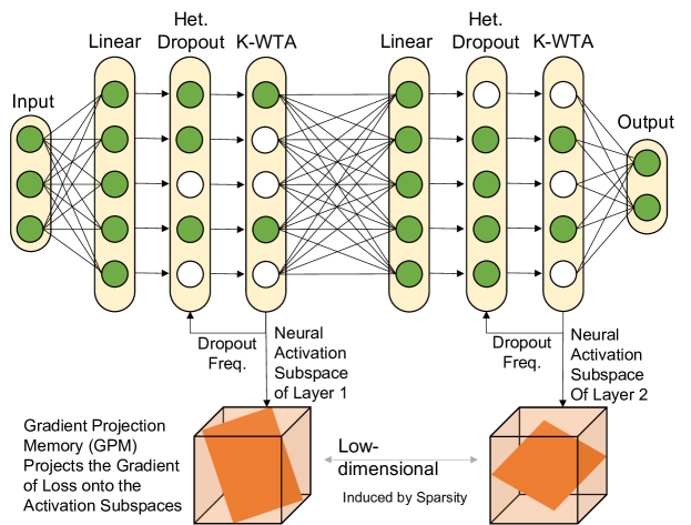
Figure 1: Depicting the overall structure of a multi layer perceptron along-with the k-winner activation and the proposed heterogeneous dropout layers.

We leverage sparsity in neural activations with the target of: 1) reducing power consumption, and 2) reducing the rank of the subspaces $S_{t}^{l}$ for $\forall t\in\mathbb{T}$ and $l\in\{2,...,L\}$. Of course, sparsity of $x^{l}_{t,i}$ does not guarantee a low rank $S_{t}^{l}$, e.g., even one-sparse activations could lead to neural activation subspaces that are full rank. However, we show numerically that neural networks trained with sparse activations often form low-dimensional activation subspace, $S_{t}^{l}$.

Sparse Activations: Following the recent work of Ahmad & Scheinkman (2019) we leverage k-winner activations to induce sparse neural representations. The framework is similar to the work of Majani et al. (1988), Makhzani & Frey (2013), and 44Srivastavacompete2compute. In short, each layer of our network follows, $x_{t,i}^{l+1}=f(W^{l}x_{t,i}^{l})$ where $f(\cdot)$ is an adaptive threshold corresponding to the $k$’th la rgest activation. Hence, only the top-$k$ activations in each layer are allowed to propagate to the next layer leading to $\|x_{t,i}^{l+1}\|_{0}\leq k$. One advantage of the k-winner framework is that we have control over the sparsity of neural activations through parameter $k$.

But why would training with the k-winner activations lead to a low-dimensional activation subspace, $S_{t}^{l}$, at the $l$’th layer for task $t$? The answer is implicitly presented in the work of Ahmad & Scheinkman (2019), where the authors observe that using k-winner activations in a network would lead to a small number of neurons that dominate the neural representation, i.e., they become active for a large percentage of input samples. This observation is also aligned with the previous observations made by Makhzani & Frey (2013) and Cui et al. (2017). Ahmad & Scheinkman (2019) view the dominance of a few neurons as a practical issue and solve this issue through a novel boosting mechanism that prioritizes the neurons with a lower frequency of activations. In our framework, however, we prefer to have a small set of dominantly active neurons in each layer of the network for each task, which translates to having a low-dimensional activation subspace, $S_{t}^{l}$. Hence, unlike the work of Ahmad & Scheinkman (2019), we do not require any boosting within a task.

Not having boosting while learning a task, could lead to dominant neurons across tasks, which could significantly reduce the overall performance of the model. To address this newly emerged practical issue in continual learning, and motivated by the approaches using non-overlapping neural representation for continual learning, we propose a conditional dropout between tasks, that encourages diverse neural activations between different tasks.

3.3 Heterogeneous Dropout

While training a network on a task, we keep track of the frequency of the neural activations. In short, we assign an activation counter per neuron, which increments when a neuron’s activation is in the top-k activations in its layer (i.e., the neuron is activated). Let $[b_{t}^{l}]_{j}$ denote the activation counter for the $j$’th neuron in the $l$’th layer of the network, after learning task $t$. Note that $[b_{t}^{l}]_{j}$ represents the number of times the j’th neuron in layer $l$ was in the top $k$ activations over all previously seen tasks $\tau\in[1,...,t]$. Then, while learning task $t+1$, we would like to encourage the network to utilize the less activated neurons. To that end, we propose a dropout (Srivastava et al., 2014) mechanism that favors to retain neurons that are less activated in previous tasks. We define a binary Bernoulli random variable, $[\delta_{t+1}^{l}]_{j}$, for the $j$’th neuron in layer $l$ during training on task $t+1$ that indicates whether the neuron is disabled by the dropout or not. In particular, we set $P([\delta_{t+1}^{l}]_{j}=1)=[p_{t+1}^{l}]_{j}$ for:

$$[p_{t+1}^{l}]_{j}=exp(-\frac{[b_{t}^{l}]_{j}}{\max_{j}[b_{t}^{l}]_{j}}\alpha)$$ (2)

where $\alpha>0$ is a hyper-parameter of our proposed dropout mechanism. Larger $P$ corresponds to less dropout and larger values of $\alpha$ lead to a more stringent enforcement of non-overlapping representations.

We call the proposed dropout a heterogeneous dropout as the probability of dropout is different for various neurons in the network. Importantly, the probability of dropout is directly correlated with the frequency of activations of a neuron for previous tasks. Hence, heterogeneous dropout will encourage the network to use non-overlapping neural activations for different tasks. Interestingly, the proposed heterogeneous dropout induces a “lifetime sparsity” of a neuron, which is well studied in the neuroscience literature (Beyeler et al., 2016).

In the following section, we first show that the k-winner framework leads to low-dimensional neural activation subspaces, $S_{t}^{l}$. We show that this low-dimensional structure enables learning more tasks with less forgetting using the GPM framework, leading to a significant performance boost. Finally, we show that our heterogeneous dropout encourages non-overlapping neural activations, which provide an additional boost in the performance of GPM over a large sequence of tasks.

4 Numerical Experiments

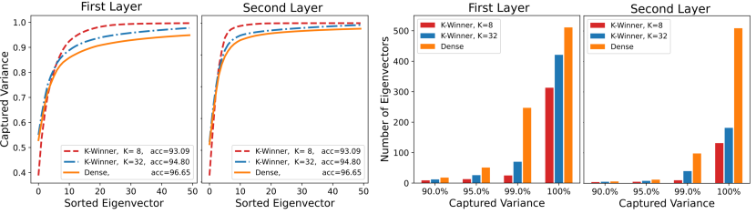
Figure 2: Demonstrating that a multi-layer perceptron, with two hidden layers of size $512$ and with k-winner activations exhibits low-dimensional neural activation subspaces, $S_{t}^{l}$, in its layers. The left column shows the captured variance as a function of top 50 eigenvalues/eigenvectors of the activations’ covariance matrix for the densely trained model (no sparsity), and the networks trained with k-winner activations for $k=8$ and $32$, in the two layers of the networks. The right column shows the approximate dimensionality of $S_{t}^{l}$ at different thresholds on captured variance, $\epsilon_{th}$, for the two layers. It can be seen that networks with k-winner activations consistently provide lower-dimensional activation subspaces (at all thresholds). The reported Accuracy is the average accuracy over all tasks at the end of the training for the last task.

4.1 Training with k-winner Activations Leads to Low-Dimensional Subspaces

Our rationale is that having low-dimensional activation subspaces, $S_{t}^{l}$, while using gradient-projection based continual learning algorithms, like GPM, would lead to less gradient projection error in learning subsequent tasks (i.e., we have a larger null-space). On the other hand, we prefer sparsely activated networks to reduce the power consumption in a continual learner. However, a network with sparse neural activations does not necessarily guarantee low-dimensional activation subspaces. In this section, as one of our core observations, we show that using the k-winner activations to learn a task leads to low-dimensional activation subspaces, $S_{t}^{l}$, at each layer of the network. Then, in the subsequent sections, we show that these low-dimensional activation subspaces lead to a significantly better learning performance on a long sequence of tasks.

We start by training a multi-layer perceptron with two hidden layers of size $512$ on the MNIST dataset (LeCun et al., 1998). We first train the model without the k-winner activations, i.e., with $k=512$, and call this model the Dense model. Next, we train the model using k-winner activations with $k=8$ and $k=32$. For each model we calculate the activations $x_{i}^{l}$ for all $i$ and for $l\in\{1,2\}$. We then calculate the Singular Value Decomposition (SVD) of $X^{l}=[x_{1}^{l},...,x_{N}^{l}]$, calculate the eigenvalues of the covariance matrix (i.e., squared singular values), and sort the eigenvectors according to their eigenvalues. Lastly, we calculate the percentage captured variance (i.e., cumulative sum of sorted eigenvalues devided by the sum of the eigenvalues) for these networks. Figure 2 visualizes the captured variance as a function of the first $50$ eigenvectors for both layers of the network for all three models. We observe that the models trained with k-winner activations lead to lower dimensional activation subspaces, $S_{t}^{l}$. Importantly, we note that Saha et al. (2020), and subsequent works, do not calculate the exact null-space of the activation subspaces, but they approximate the null-space by zeroing out the eigenvalues that capture a small percentage of the variance. This is done via thresholding the captured variance at $0<\epsilon_{th}\leq 1$. Note that the exact null-space may be very small due to very small but non-zero eignevalues. To that end, we show that for various thresholds of the captured variances, i.e., $\epsilon_{th}\in\{0.90,0.95,0.99,1.00\}$, the networks using k-winner activations require fewer eigenvectors. Finally, the low-dimensional activation subspaces are achieved without a major loss in the accuracy of the trained networks.

4.2 Heterogeneous Dropout for non-overlapping representations

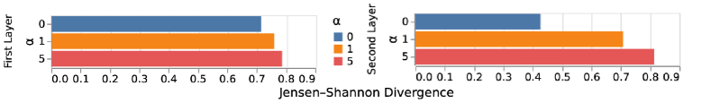
Figure 3: The Jensen-Shannon divergence (JSD in (3)) between activations’ probability mass functions, $q^{l}_{1}$ and $q^{l}_{2}$, for $l\in\{1,2\}$. The plot quantifies the overlap between neural activations of two tasks as a function of our dropout hyperparameter $\alpha$ (See (2)). Higher JSD values mean lower overlap. We can see that we are able to decrease the overlap between neural activations by increasing $\alpha$ ($\alpha=0$ results in no dropout).

Here we numerically confirm that our heterogeneous dropout leads to fewer overlaps between neural representations of different tasks. For these experiments, we use the GPM algorithm on a model with k-winner activations and learn two tasks from Permuted-MNIST sequentially, where the first task is MNIST and the second task is a permuted version. After training on Task 1, we calculate the number of times each neuron is activated for all samples in the validation set of Task 1. Then, we learn Task 2 using gradient-projection and afterwards calculate the number of times each neuron is activated for all samples in the validation set of Task 2. For task $t$ and for the $j$’th neuron in layer $l$, we denote the neural activations on the validation set as $[\nu^{l}_{t}]_{j}$. Note that $\nu^{l}_{t}$ is different from $b_{t}^{l}$ introduced in Subsection 3.3, as it is calculated on the validation set (as opposed to the training set), and it is calculated per task, while $b_{t}^{l}$ is the accumulation of activations over all tasks. Let $\bar{\nu}_{t}^{l}=\sum_{j=1}^{d_{l}}[\nu_{t}^{l}]_{j}$ where $d_{l}$ is the number of neurons in the $l$’th layer, then we can define a probability mass function of activations for each layer as $[q^{l}_{t}]_{j}=[\nu^{l}_{t}]_{j}/\bar{\nu}^{l}_{t}$. Finally, we measure the neural activation overlap between tasks $t_{1}$ and $t_{2}$, via the Jensen-Shannon divergence (i.e., the symmetric KL-divergence) between their neural activation probability mass functions, i.e,:

$$JSD(q^{l}_{t_{1}}||q^{l}_{t_{2}})=\frac{1}{2}\sum_{j}q^{l}_{t_{1}}log(\frac{2q^{l}_{t_{1}}}{q^{l}_{t_{1}}+q^{l}_{t_{2}}})+\frac{1}{2}\sum_{j}q^{l}_{t_{2}}log(\frac{2q^{l}_{t_{2}}}{q^{l}_{t_{1}}+q^{l}_{t_{2}}})$$ (3)

Figure 3 measures the overlap between neural representations (between Task 1, MNIST, and Task 2, a Permuted MNIST) when the networks are trained with and without our heterogeneous dropout and for different values of $\alpha$. Higher Jensen-Shannon divergence means less overlap. In short, $\alpha=0$ means no dropout, and we confirm that higher $\alpha$ translates to less overlap (higher JS-divergence) between the neural representations. Finally, we note that the choice of $\alpha$ truly depends on the amount of forward transfer we expect to see between two tasks. Lower values of $\alpha$ are beneficial when we expect our network to rely more on previously learned features (i.e., forward transfer from previous tasks), while higher values are preferred to learn new features for the new task.

In what follows, we combine k-winner sparse activations with our heterogeneous dropout, utilize Gradient Projection Memory (GPM) as our core continual learning algorithm, and demonstrate the benefits of sparsity and non-overlapping representations in learning long sequences of tasks in GPM.

4.3 Continual Swiss Roll

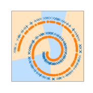
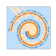
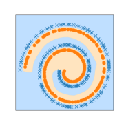
(a) Continuous Swiss Roll	(b) GPM	(c) GPM+K	(d) Multi Task

Figure 4: The Continual Swiss Roll dataset consisting of 50 binary classification tasks (a) and the final decision boundaries of different methods, after having learned the 50 tasks sequentially (b)-(d). GPM+K denotes GPM with k-winner activations. We note that contrary to permuted-MNIST, and due to the high level of similarity between consecutive tasks, adding heterogeneous dropout does not improve the performance.

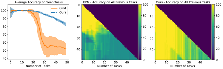
Figure 5: Performance analysis of GPM in comparison with our proposed method on the Continual Swiss Roll dataset with 50 tasks (as seen in Figure 4). The results are averaged over 10 runs.

In this section, we first introduce Continual Swiss Roll as a lightweight and easily interpretable, yet challenging, synthetic benchmark for continual learning. Continual Swiss Roll is generated from two classes of two-dimensional Swiss rolls, where the dataset is shattered into $T$ binary classification tasks according to their angular positions on the roll (See Figure 4 (a)). The continual learner needs to solve the overall Swiss roll binary classification problem by only observing the sequence of tasks. In addition to being simple and interpretable, one can arbitrarily increase the number of tasks and there is also an inherent notion of similarity between tasks in our proposed Continual Swiss Roll (according to their angular location).

Here, we consider a Continual Swiss Roll problem with $T=50$ binary classification tasks. We use two single-head multi-layer perceptrons with two hidden layers of size $1024$, one using Rectified-Linear Unit (ReLU) activations (i.e., Dense) and the other using the k-winner activations with $k=64$. For this problem, we set $\alpha=0$, as the consecutive tasks share much similarities, and we would like to get forward transfer. We solve the continual learning using GPM. Figure 4 shows the learned decision boundaries after learning the 50’th task for GPM, and for our proposed method (i.e., GPM+k-winner). We see that adding sparse activations lead to a significant boost in performance and a much better preservation of the decision boundary in long sequences of tasks. We repeat this experiment $10$ times and report the average and standard deviation of the test accuracy over all seen tasks as a function of number of tasks in Figure 5. In addition, in Figure 5, we show the test accuracy of the current task as well as all previous tasks after learning each new task, as a lower triangular $50\times 50$ matrix for both methods. The $(t_{1},t_{2})$ element of this lower-triangular matrix contain the test accuracy of the model on Task $t_{1}$ immediately after training it on Task $t_{2}$. We see that the network with k-winner activations not only preserves the performance on old tasks better, but also leads to learning new tasks better. Figure 4 shows the final decision boundaries (after learning the 50th task) learned with GPM, GPM+k-winner activations (ours), and the multitask learner (i.e., joint training).

4.4 Permuted-MNIST

	Perm-MNIST (20 Tasks)
	Accuracy	BT
EWC (Kirkpatrick et al., 2017)	64.53	-24.70
ER (Rolnick et al., 2018)	78.63	-21.81
GPM (Saha et al., 2020)	81.23	-14.70
AGEM (Chaudhry et al., 2018)	85.54	-14.33
GEM (Lopez-Paz & Ranzato, 2017b)	91.28	-8.07
GPM + K + HD (Ours)	89.74	-1.62

	Perm-MNIST (50 Tasks)
	Accuracy	BT
GPM	36.56 $\pm$ 0.69	-54.28 $\pm$ 0.75
GPM + K	54.96 $\pm$ 1.92	-31.03 $\pm$ 1.76
GPM + RD	33.60 $\pm$ 1.40	-50.85 $\pm$ 1.63
GPM + HD	28.30 $\pm$ 2.02	-20.55 $\pm$ 2.27
GPM + K + RD	52.90 $\pm$ 2.48	-27.52 $\pm$ 2.15
GPM + K + HD	61.09 $\pm$ 0.87	-21.57 $\pm$ 0.39

Table 1: Final accuracy and backward transfer on Permuted-MNIST with 20 tasks, for benchmark approaches vs our proposed approach (left). Ablation study on 50 tasks of Permuted-MNIST, averaged over 5 runs. Abbreviations correspond to: K (k-winner), RD (Random Dropout), and HD (Heterogeneous Dropout). Our method (GPM + K + HD) achieves the highest accuracy and comparable backward transfer to other combinations of modules (right)

Here, we perform our experiments on the Permuted-MNIST continual learning benchmark with $50$ tasks. Each of the 50 Permuted-MNIST tasks is a 10-classes classification problem obtained from a random permutation (fixed for all images of a task) of the MNIST dataset, where the pixels in each figure are permuted according to the permutation rule. For our models, similar to the models used in Section 4.1, we use multi-layer perceptron with two hidden layers of size $512$, and with ReLU activations (i.e., dense resulting in GPM), and with k-winner activations for $k=8$ and $32$. For dropout, we use $\alpha=24/k$ (i.e., $3$ for $k=8$ and $0.75$ for $k=32$).

Figure 6 (left) shows the average accuracy of the models on previously seen tasks, as a function of the number of tasks. The results are aggregated from 5 runs. We can see that our proposed networks with k-winner sparsity and heterogeneous dropout significantly out-perform the GPM algorithm applied to a dense model. In addition to GPM, we compared our method to some of the benchmark algorithms in the literature including Elastic Weight Consolidation (Kirkpatrick et al., 2017), Experience Replay (Rolnick et al., 2018), Gradient Episodic Memory (Lopez-Paz & Ranzato, 2017a), and Averaged Gradient Episodic Memory (Chaudhry et al., 2018) on 20 Task Permuted-MNIST. Table 1 shows the results of the benchmark algorithms compared to ours. We generate the results of other methods using the wonderful code repository provided by Lomonaco et al. (2021); Lin et al. (2021).

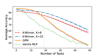
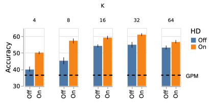
Figure 6: The results of our proposed approach with k-winner sparsity and heterogeneous dropout on the Permuted-MNIST continual learning benchmark with $50$ tasks (a). An ablation study quantifying the effect of sparsity and heterogeneous dropout in learning 50 Permuted-MNIST tasks. We see that sparsity and our heterogeneous dropout contribute to the performance boost in a complementary manner.

Lastly, we performed various ablation studies to shed light on the effect of each proposed component. First, we look at the effect of $k$ in the k-winner activations on our 50-tasks permuted-MNIST experiment with and without heterogeneous dropout and compare it with vanilla GPM. The results of this experiment are reported in Figure 6 (right). This experiment demonstrates that both sparsity and heterogeneous dropout play critical roles in improving the performance of GPM when learning a long sequence of tasks. To further provide insights into the performance of the proposed components, we ran a full ablation study with $k=32$, and also compared our proposed heterogeneous dropout with random dropout. The results of our full ablation study for this problem is shown in Table 1.

4.5 CIFAR-100

	CIFAR-100 Super Class (5 Tasks)		SuperDog-40 (8 Tasks)
	Accuracy	BT	Accuracy	BT
GPM	28.84 $\pm$ 0.64	-22.51 $\pm$ 1.06	39.66 $\pm$ 1.06	-29.88 $\pm$ 1.30
GPM + K	26.57 $\pm$ 0.74	-18.60 $\pm$ 0.95	37.91 $\pm$ 1.79	-25.73 $\pm$ 1.69
GPM + RD	24.86 $\pm$ 0.51	-23.34 $\pm$ 0.74	38.72 $\pm$ 2.33	-32.61 $\pm$ 3.11
GPM + K + RD	17.55 $\pm$ 0.68	-11.87 $\pm$ 0.68	36.73 $\pm$ 1.51	-24.28 $\pm$ 2.19
GPM + K + HD	29.77 $\pm$ 0.41	-9.55 $\pm$ 0.38	42.58 $\pm$ 0.76	-23.17 $\pm$ 1.58
GPM + HD	32.11 $\pm$ 0.71	-11.09 $\pm$ 0.79	42.82 $\pm$ 0.96	-26.60 $\pm$ 2.05

Table 2: Averaged final accuracy and backward transfer (over 5 runs) of an experiment on five 20-superclass classification tasks on CIFAR-100 (middle) and eight 5-superclass classification tasks on SuperDog-40 (right). Both experiments use a single-head AlexNet as their backbone. Since AlexNet has random dropout in its architecture, GPM and GPM + RD correspond to AlexNet without dropout and regular AlexNet, respectively.

In this section, we extend our results on MLPs to Convolutional Neural Networks (CNNs), and demonstrate the practicality of the k-winner activations and Heterogeneous Dropout beyond MLP architectures. We first point out that many of the existing benchmarks in the continual learning literature, e.g., split CIFAR-10, or split CIFAR-100, contain few tasks and do not really reflect the scalability issues of the existing approaches with respect to the number of tasks. Moreover, the majority of the existing approaches focus on multi-head neural architectures, while the arguably more challenging ‘domain incremental learning’ Van de Ven & Tolias (2019) remains comparably understudied. Following the work of Ramasesh et al. (2021), here we use the ‘distribution shift CIFAR-100’ as a domain incremental continual learning setting with five tasks. Each task, in this setting, is a 20-class classification problem, which contains one subclass from each superclass. We used AlexNet Krizhevsky et al. (2012) as our backbone. Table 2 shows our results for this experiment. We observe that AlexNet with Heterogeneous Dropout outperforms other networks. We also noticed that k-winner activations combined with Heterogeneous Dropout results in the least amount of forgetting at the cost of a slight drop in the accuracy.

4.6 ImageNet SuperDog-40

Here, we introduce ImageNet SuperDog-40 as an effective continual learning benchmark for domain incremental learning. SuperDog-40 is a subset of ImageNet Deng et al. (2009) with images from $40$ dog breed classes. These dog breeds belong to five superclasses, namely 1) sporting dog, 2) terrier, 3) hound, 4) toy dog, and 5) working dog, resulting in eight five-way classification tasks. Similar to the ‘domain shift CIFAR-100’ experiment, here we use an AlexNet to learn these 8 tasks. The results are shown in Table 2. Consistent with our results on CIFAR-100, here we observe that the models containing Heterogeneous Dropouts and k-winner activations are the two top performers.

5 Conclusion

This paper studied the effects of sparsity and non-overlapping neural representations in the Gradient projection memory (GPM) framework in continual learning. In addition to providing a power-efficient sparsely activated network, we showed that a network trained with k-winner activations has low-dimensional neural activation subspaces. The low-dimensionality of the neural activation subspaces translates to having a large null-space, which leads to lower gradient projection error for learning new tasks in GPM. Moreover, we proposed a heterogeneous dropout mechanism, which encourages non-overlapping patterns of neural activations between tasks. We showed that heterogeneous dropout complements the $k$-sparse activations of the k-winner framework and significantly improves performance when using the GPM algorithm to learn a long sequence of tasks. We introduced Continual Swiss Roll and ImageNet SuperDog-40 as two benchmark problems for domain incremental learning. Continual Swiss Roll is a lightweight and interpretable yet challenging, continual learning synthetic benchmark, while ImageNet SuperDog-40 is a subset of ImageNet with hand-picked dog images from 40 different breeds that belong to 5 superclasses. Finally, we analyze our proposed approach on the Continual Swiss Roll, Permuted-MNIST, CIFAR-100, and ImageNet SuperDog-40 datasets and provide an ablation study to clarify the contribution of each proposed component.

6 Acknowledgement

SK and HP were supported by the Defense Advanced Research Projects Agency (DARPA) under Contract No. HR00112190135. VB was supported by DARPA under Contract No. HR00112190130.

References

- li2 (2021) Lifelong Learning with Sketched Structural Regularization, volume 157 of Proceedings of Machine Learning Research, 2021. PMLR.
- Ahmad & Scheinkman (2019) Subutai Ahmad and Luiz Scheinkman. How can we be so dense? the benefits of using highly sparse representations. arXiv preprint arXiv:1903.11257, 2019.
- Aljundi et al. (2018a) Rahaf Aljundi, Francesca Babiloni, Mohamed Elhoseiny, Marcus Rohrbach, and Tinne Tuytelaars. Memory aware synapses: Learning what (not) to forget. In ECCV, 2018a.
- Aljundi et al. (2018b) Rahaf Aljundi, Marcus Rohrbach, and Tinne Tuytelaars. Selfless sequential learning. In International Conference on Learning Representations, 2018b.
- Beyeler et al. (2016) Michael Beyeler, Nikil Dutt, and Jeffrey L Krichmar. 3d visual response properties of mstd emerge from an efficient, sparse population code. Journal of Neuroscience, 36(32):8399–8415, 2016.
- Chaudhry et al. (2018) Arslan Chaudhry, Marc’Aurelio Ranzato, Marcus Rohrbach, and Mohamed Elhoseiny. Efficient lifelong learning with a-gem. In International Conference on Learning Representations, 2018.
- Chaudhry et al. (2020) Arslan Chaudhry, Naeemullah Khan, Puneet Dokania, and Philip Torr. Continual learning in low-rank orthogonal subspaces. Advances in Neural Information Processing Systems, 33:9900–9911, 2020.
- Chen et al. (2018) Yuanyuan Chen, Lei Zhang, and Zhang Yi. Subspace clustering using a low-rank constrained autoencoder. Information Sciences, 424:27–38, 2018.
- Cui et al. (2017) Yuwei Cui, Subutai Ahmad, and Jeff Hawkins. The htm spatial pooler—a neocortical algorithm for online sparse distributed coding. Frontiers in computational neuroscience, pp. 111, 2017.
- Delange et al. (2021) Matthias Delange, Rahaf Aljundi, Marc Masana, Sarah Parisot, Xu Jia, Ales Leonardis, Greg Slabaugh, and Tinne Tuytelaars. A continual learning survey: Defying forgetting in classification tasks. IEEE Transactions on Pattern Analysis and Machine Intelligence, 2021.
- Deng et al. (2021) Danruo Deng, Guangyong Chen, Jianye HAO, Qiong Wang, and Pheng-Ann Heng. Flattening sharpness for dynamic gradient projection memory benefits continual learning. In A. Beygelzimer, Y. Dauphin, P. Liang, and J. Wortman Vaughan (eds.), Advances in Neural Information Processing Systems, 2021. URL https://openreview.net/forum?id=q1eCa1kMfDd.
- Deng et al. (2009) Jia Deng, Wei Dong, Richard Socher, Li-Jia Li, Kai Li, and Li Fei-Fei. Imagenet: A large-scale hierarchical image database. In 2009 IEEE conference on computer vision and pattern recognition, pp. 248–255. Ieee, 2009.
- Farajtabar et al. (2020) Mehrdad Farajtabar, Navid Azizan, Alex Mott, and Ang Li. Orthogonal gradient descent for continual learning. In International Conference on Artificial Intelligence and Statistics, pp. 3762–3773. PMLR, 2020.
- Farquhar & Gal (2018) Sebastian Farquhar and Yarin Gal. Towards robust evaluations of continual learning. arXiv preprint arXiv:1805.09733, 2018.
- French (1991) Robert M French. Using semi-distributed representations to overcome catastrophic forgetting in connectionist networks. In Proceedings of the 13th annual cognitive science society conference, volume 1, pp. 173–178, 1991.
- French (1999) Robert M French. Catastrophic forgetting in connectionist networks. Trends in cognitive sciences, 3(4):128–135, 1999.
- Gong et al. (2022) Dong Gong, Qingsen Yan, Yuhang Liu, Anton van den Hengel, and Javen Qinfeng Shi. Learning bayesian sparse networks with full experience replay for continual learning. arXiv preprint arXiv:2202.10203, 2022.
- Guo et al. (2018) Yiwen Guo, Chao Zhang, Changshui Zhang, and Yurong Chen. Sparse dnns with improved adversarial robustness. Advances in neural information processing systems, 31, 2018.
- Jung et al. (2020) Sangwon Jung, Hongjoon Ahn, Sungmin Cha, and Taesup Moon. Continual learning with node-importance based adaptive group sparse regularization. Advances in Neural Information Processing Systems, 33:3647–3658, 2020.
- Kirkpatrick et al. (2017) James Kirkpatrick, Razvan Pascanu, Neil Rabinowitz, Joel Veness, Guillaume Desjardins, Andrei A Rusu, Kieran Milan, John Quan, Tiago Ramalho, Agnieszka Grabska-Barwinska, et al. Overcoming catastrophic forgetting in neural networks. Proceedings of the national academy of sciences, 114(13):3521–3526, 2017.
- Kolouri et al. (2020) Soheil Kolouri, Nicholas A Ketz, Andrea Soltoggio, and Praveen K Pilly. Sliced cramer synaptic consolidation for preserving deeply learned representations. In International Conference on Learning Representations, 2020.
- Krizhevsky et al. (2012) Alex Krizhevsky, Ilya Sutskever, and Geoffrey E Hinton. Imagenet classification with deep convolutional neural networks. Advances in neural information processing systems, 25, 2012.
- LeCun et al. (1998) Yann LeCun, Léon Bottou, Yoshua Bengio, and Patrick Haffner. Gradient-based learning applied to document recognition. Proceedings of the IEEE, 86(11):2278–2324, 1998.
- Lennie (2003) Peter Lennie. The cost of cortical computation. Current biology, 13(6):493–497, 2003.
- Lin et al. (2022) Sen Lin, Li Yang, Deliang Fan, and Junshan Zhang. TRGP: Trust region gradient projection for continual learning. In International Conference on Learning Representations, 2022. URL https://openreview.net/forum?id=iEvAf8i6JjO.
- Lin et al. (2021) Zhiqiu Lin, Jia Shi, Deepak Pathak, and Deva Ramanan. The CLEAR benchmark: Continual LEArning on real-world imagery. In Thirty-fifth Conference on Neural Information Processing Systems Datasets and Benchmarks Track (Round 2), 2021. URL https://openreview.net/forum?id=43mYF598ZDB.
- Lomonaco et al. (2021) Vincenzo Lomonaco, Lorenzo Pellegrini, Andrea Cossu, Antonio Carta, Gabriele Graffieti, Tyler L Hayes, Matthias De Lange, Marc Masana, Jary Pomponi, Gido M Van de Ven, et al. Avalanche: an end-to-end library for continual learning. In Proceedings of the IEEE/CVF Conference on Computer Vision and Pattern Recognition, pp. 3600–3610, 2021.
- Lopez-Paz & Ranzato (2017a) David Lopez-Paz and Marc’Aurelio Ranzato. Gradient episodic memory for continual learning. In Proceedings of the 31st International Conference on Neural Information Processing Systems, NIPS’17, pp. 6470–6479, USA, 2017a. Curran Associates Inc. ISBN 978-1-5108-6096-4.
- Lopez-Paz & Ranzato (2017b) David Lopez-Paz and Marc’Aurelio Ranzato. Gradient episodic memory for continual learning. Advances in neural information processing systems, 30:6467–6476, 2017b.
- Majani et al. (1988) E Majani, Ruth Erlanson, and Yaser Abu-Mostafa. On the k-winners-take-all network. Advances in neural information processing systems, 1, 1988.
- Makhzani & Frey (2013) Alireza Makhzani and Brendan Frey. K-sparse autoencoders. arXiv preprint arXiv:1312.5663, 2013.
- Mallya & Lazebnik (2018) Arun Mallya and Svetlana Lazebnik. Packnet: Adding multiple tasks to a single network by iterative pruning. In Proceedings of the IEEE conference on Computer Vision and Pattern Recognition, pp. 7765–7773, 2018.
- Mallya et al. (2018) Arun Mallya, Dillon Davis, and Svetlana Lazebnik. Piggyback: Adapting a single network to multiple tasks by learning to mask weights. In Proceedings of the European Conference on Computer Vision (ECCV), pp. 67–82, 2018.
- Masse et al. (2018) Nicolas Y Masse, Gregory D Grant, and David J Freedman. Alleviating catastrophic forgetting using context-dependent gating and synaptic stabilization. Proceedings of the National Academy of Sciences, 115(44):E10467–E10475, 2018.
- Mirzadeh et al. (2020) Seyed Iman Mirzadeh, Mehrdad Farajtabar, and Hassan Ghasemzadeh. Dropout as an implicit gating mechanism for continual learning. In Proceedings of the IEEE/CVF Conference on Computer Vision and Pattern Recognition Workshops, pp. 232–233, 2020.
- Mundt et al. (2020) Martin Mundt, Yong Won Hong, Iuliia Pliushch, and Visvanathan Ramesh. A wholistic view of continual learning with deep neural networks: Forgotten lessons and the bridge to active and open world learning. arXiv preprint arXiv:2009.01797, 2020.
- Parisi et al. (2019) German I Parisi, Ronald Kemker, Jose L Part, Christopher Kanan, and Stefan Wermter. Continual lifelong learning with neural networks: A review. Neural Networks, 113:54–71, 2019.
- Ramasesh et al. (2021) Vinay Venkatesh Ramasesh, Ethan Dyer, and Maithra Raghu. Anatomy of catastrophic forgetting: Hidden representations and task semantics. In International Conference on Learning Representations, 2021. URL https://openreview.net/forum?id=LhY8QdUGSuw.
- Rolnick et al. (2018) David Rolnick, Arun Ahuja, Jonathan Schwarz, Timothy P Lillicrap, and Greg Wayne. Experience replay for continual learning. arXiv preprint arXiv:1811.11682, 2018.
- Rolnick et al. (2019) David Rolnick, Arun Ahuja, Jonathan Schwarz, Timothy Lillicrap, and Gregory Wayne. Experience replay for continual learning. Advances in Neural Information Processing Systems, 32, 2019.
- Rostami et al. (2020) Mohammad Rostami, Soheil Kolouri, Praveen Pilly, and James McClelland. Generative continual concept learning. In Proceedings of the AAAI Conference on Artificial Intelligence, volume 34, pp. 5545–5552, 2020.
- Saha et al. (2020) Gobinda Saha, Isha Garg, and Kaushik Roy. Gradient projection memory for continual learning. In International Conference on Learning Representations, 2020.
- Sanyal et al. (2019) Amartya Sanyal, Varun Kanade, and Philip H. Torr. Intriguing properties of learned representations, 2019. URL https://openreview.net/forum?id=SJzvDjAcK7.
- Schwarz et al. (2018) Jonathan Schwarz, Wojciech Czarnecki, Jelena Luketina, Agnieszka Grabska-Barwinska, Yee Whye Teh, Razvan Pascanu, and Raia Hadsell. Progress & compress: A scalable framework for continual learning. In International Conference on Machine Learning, pp. 4528–4537. PMLR, 2018.
- Schwarz et al. (2021) Jonathan Schwarz, Siddhant Jayakumar, Razvan Pascanu, Peter Latham, and Yee Teh. Powerpropagation: A sparsity inducing weight reparameterisation. Advances in Neural Information Processing Systems, 34, 2021.
- Shin et al. (2017) Hanul Shin, Jung Kwon Lee, Jaehong Kim, and Jiwon Kim. Continual learning with deep generative replay. In Proceedings of the 31st International Conference on Neural Information Processing Systems, pp. 2994–3003, 2017.
- Srivastava et al. (2014) Nitish Srivastava, Geoffrey Hinton, Alex Krizhevsky, Ilya Sutskever, and Ruslan Salakhutdinov. Dropout: a simple way to prevent neural networks from overfitting. The journal of machine learning research, 15(1):1929–1958, 2014.
- Van de Ven & Tolias (2019) Gido M Van de Ven and Andreas S Tolias. Three scenarios for continual learning. arXiv preprint arXiv:1904.07734, 2019.
- von Oswald et al. (2019) Johannes von Oswald, Christian Henning, João Sacramento, and Benjamin F Grewe. Continual learning with hypernetworks. arXiv preprint arXiv:1906.00695, 2019.
- Wang et al. (2021) Shipeng Wang, Xiaorong Li, Jian Sun, and Zongben Xu. Training networks in null space of feature covariance for continual learning. In Proceedings of the IEEE/CVF Conference on Computer Vision and Pattern Recognition, pp. 184–193, 2021.
- Wortsman et al. (2020) Mitchell Wortsman, Vivek Ramanujan, Rosanne Liu, Aniruddha Kembhavi, Mohammad Rastegari, Jason Yosinski, and Ali Farhadi. Supermasks in superposition. Advances in Neural Information Processing Systems, 33:15173–15184, 2020.
- Yu et al. (2014) Yuguo Yu, Michele Migliore, Michael L Hines, and Gordon M Shepherd. Sparse coding and lateral inhibition arising from balanced and unbalanced dendrodendritic excitation and inhibition. Journal of Neuroscience, 34(41):13701–13713, 2014.
- Zenke et al. (2017) Friedemann Zenke, Ben Poole, and Surya Ganguli. Continual learning through synaptic intelligence. In International Conference on Machine Learning, pp. 3987–3995. PMLR, 2017.