Distributed Community Detection in Large Networks

Abstract

Community detection for large networks is a challenging task due to the high computational cost as well as the heterogeneous community structure. Stochastic block model (SBM) is a popular model to analyze community structure where nodes belonging to the same communities are connected with equal probability. Modularity optimization methods provide a fast and effective way for community detection under SBM with assortative community structure, where nodes within communities are densely connected and nodes across communities are relatively loosely connected. However, the non-assortative community structure, where nodes across communities are densely connected, widely exists in real-world networks, thus leading to the inconsistency of modularity optimization methods in applications. In this paper, we consider networks with “grouped communities” (or “the group structure”), where nodes within grouped communities are densely connected and nodes across grouped communities are relatively loosely connected, while nodes belonging to the same group but different communities can be either densely or loosely connected. We incorporate the group structure in the SBM and propose a novel divide-and-conquer algorithm to detect the community structure. We show that the proposed method can recover both the group structure and the community structure asymptotically. Numerical studies demonstrate that the proposed method can reduce the computational cost significantly while still achieving competitive performance. Further, we extend the proposed framework from the SBM to the degree-corrected SBM for more general applications.

Keywords: community detection, divide and conquer, large networks, modularity, spectral clustering, stochastic block model

1 Introduction

For many real-world networks, such as social networks, airline route networks, and citation networks (Egghe and Rousseau, 1990), the community structure is commonly observed as functional modules, i.e., nodes belonging to the same community share similar connectivity patterns. Finding such community structure can be useful for exploring, modeling, and interpreting networks (Rohe et al., 2011). The stochastic block model (SBM) (Holland et al., 1983; Snijders and Nowicki, 1997) has been widely used for modeling the community structure in networks and has shown appealing empirical and theoretical properties. Community detection based on the SBM is a nontrivial task, as optimizing the likelihood function over all possible community labels is an NP-hard problem (Bickel and Chen, 2009). Various algorithms have been developed for community detection based on the SBM in the literature. For example, Daudin et al. (2008) considered the variational EM algorithm by optimizing the community assignment and probability matrix iteratively. Rohe et al. (2011) proposed the spectral clustering algorithm by analyzing the Laplacian of the adjacency matrix for high-dimensional SBM. Amini et al. (2013) proposed pseudo-likelihood based algorithm for network community detection task. However, when dealing with very large networks, the computational cost is often too high and causes challenges. In the variational EM method, each EM update requires $O(n^{2})$ computations (Snijders and Nowicki, 1997; Handcock et al., 2007), where $n$ is the number of nodes in the network; for the spectral clustering method, the complexity for each iteration is $O(mK+nK^{2})$, where $m$ is the number of edges and $K$ is the number of communities (White and Smyth, 2005); and pseudo-likelihood algorithm lacks the guarantee of convergence (Wang et al., 2020). Besides, if the size of communities is unknown, selecting number of communities also requires high computational cost. For example, Wang and Bickel (2017) showed that directly using likelihood-based model selection method requires an exponential number of summands and would become intractable as $n$ grows. Even with variational likelihood EM update algorithm, each step will requires $O(n^{2})$ computations. Note that these methods all work and only work with the entire network. To overcome the computational burden for community detection in large networks, a natural idea is to first divide the large network into several sub-networks, and then communities are detected within each sub-network in a parallel way. However, a key question is how to divide the large network into sub-networks in a sensible way. The random division would break the community structure and lead to erroneous community detection results.

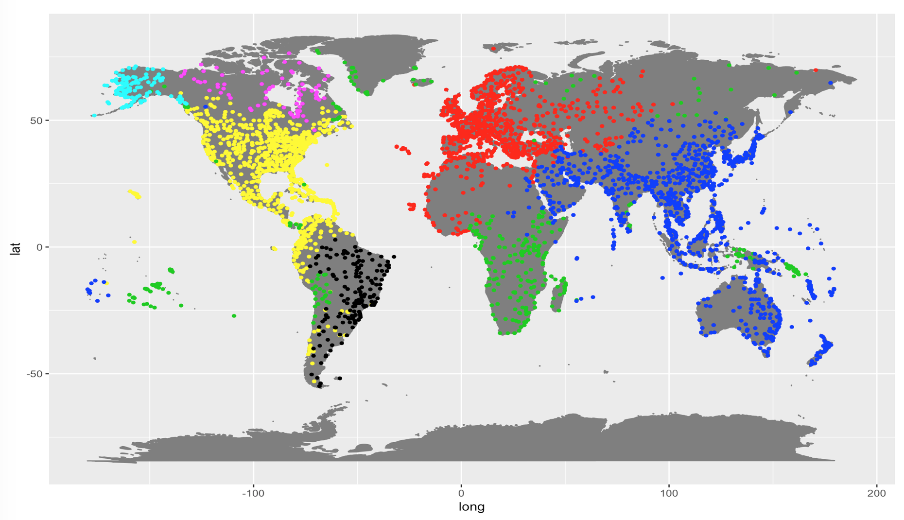
In many real-world applications, it has often been observed that communities in large networks can be divided into groups such that nodes (or communities) within the same group have relatively high link probabilities while nodes (or communities) in different groups have much lower link probabilities. One such example is the airline route network which contains routes among airports spanning the globe. It can be seen that the group structure in the airline route network corresponds to geographical regions, where connections within the same region are much denser than connections across regions. Within each region (group), the airports are further divided into communities depending on connections due to different levels of economies, areas or politics. See Section 6.1 for more details.

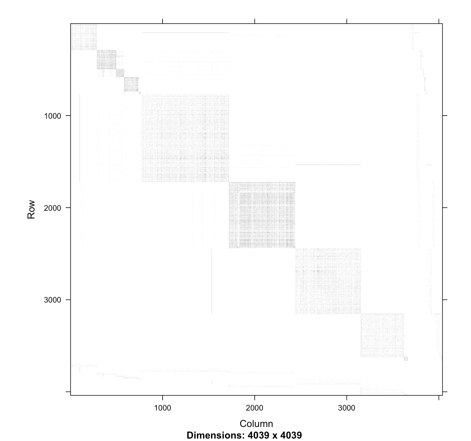
Another illustrative example is the Facebook ego network, which is created based on the “friend lists” of 10 ego people (see Figure 8 in Appendix). Naturally, people connected to the same ego person have higher link probabilities among themselves than to people connected to different ego persons. Therefore, it is reasonable to assume 10 groups are corresponding to the 10 ego people in the Facebook ego network. Within each group, people could belong to different friend circles (communities), such as the colleague circle, the family circle, the classmate circle, etc, of the ego person. See Section 6.2 for more details.

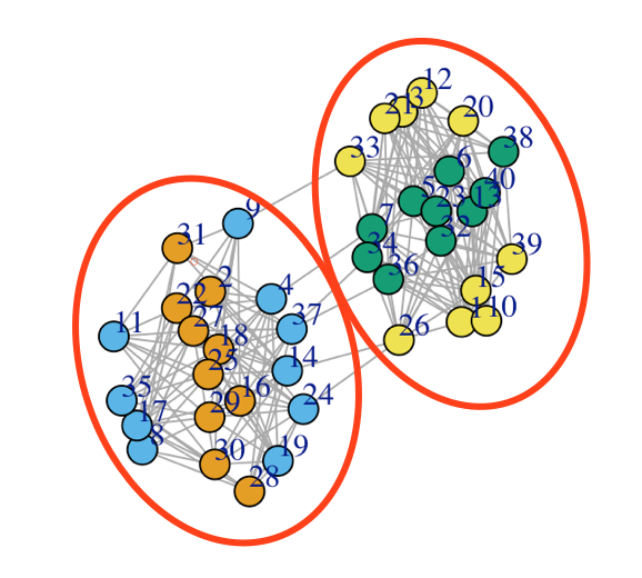
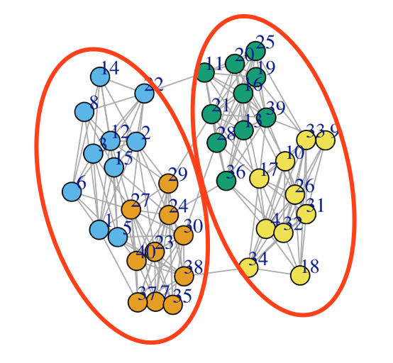
In this paper, we consider large networks with a “grouped community structure”. An illustration of the “grouped community structure” is shown in Figure 1(a) and (b), where the network consists of four communities, with the green and the yellow communities belonging to one group and the orange and blue communities belonging to the other group. The groups are such that nodes (or communities) within each group have much denser links than those from different groups. In Figure 1(a), communities within the same group are disassortative, while Figure 1(b) shows an example that communities within the same group are assortative. Our goal is to first divide the large network into sub-networks according to the group structure of the network so that it does not break the community structure within each group during the division, and then apply community detection methods to each group for identifying communities.

(a)

(b)

Figure 1: An illustration for the grouped community structure: the yellow and the green communities belong to the same group; the orange and blue communities are in another group. In panel (a), communities within the same group are non-assortative (links are dense across communities); and in panel (b), communities within the same group are assortative (links are dense within communities).

Towards this goal, we adopt a division method by optimizing the modularity (Newman and Girvan, 2004), which is a widely used measure for the strength of division of a network into groups. Specifically, modularity is defined as the fraction of edges that fall within the divided groups minus the expected fraction if edges were distributed at random (Newman, 2012). The larger the modularity, the divided groups will have denser connections within the groups but sparser connections between the groups. Many modularity optimization algorithms, such as the edge-betweenness method (Newman and Girvan, 2004), the fast-greedy method (Blondel et al., 2008) and the exhaustive modularity optimization via simulated annealing method (Guimera et al., 2004), have been developed to divide a network into groups. These methods are usually model-free and can be implemented efficiently for large networks. For example, the computational cost for the fast greedy algorithm is $O(n\hbox{log}^{2}n)$, which is nearly linear in the size $n$ (Fortunato and Hric, 2016).

Although the modularity optimization methods are computationally efficient, they can not be used to recover the refined community structure within groups since communities within the same group may have relatively more non-assortative links. This motivates us to propose a novel divide-and-conquer scheme for distributed community detection for large networks. Specifically, we propose to first divide a large network into groups using the modularity-based method and then conduct community detection using the model-based method within each group. We show that our proposed divide-and-conquer method can estimate the community labels consistently for networks with the group structure under certain conditions.

The remainder of the paper is organized as follows. In Section 2, we describe in detail the SBM with the grouped community structure. In Section 3, we present the proposed distributed community detection algorithm. Theoretical properties of the proposed distributed community detection algorithm and extension to the Degree-Corrected SBM (DCSBM) are given in Section 4. In Section 5, we conduct simulation studies to examine the performance of the proposed method and compare it with other community detection methods. In Section 6, we apply the proposed method to an airline route network and a Facebook ego network. We conclude the paper with discussions in Section 7. All technical proofs are provided in the Appendix.

2 SBM with Grouped Community Structure

Consider an undirected and unweighted network ${\bm{\mathbf{N}}}=({\bm{\mathbf{V}}},{\bm{\mathbf{A}}})$, where ${\bm{\mathbf{V}}}=\{v_{1},v_{2},...,v_{n}\}$ is the set of nodes and ${\bm{\mathbf{A}}}=(A_{ij})$ is the adjacency matrix with $A_{ij}=1$ representing a link between nodes $v_{i}$ and $v_{j}$, and 0 otherwise. Specifically, first, we assume that the node set $\{v_{1},v_{2},...,v_{n}\}$ can be partitioned into $G$ disjoint groups $\mathcal{G}_{1},\mathcal{G}_{2},...,\mathcal{G}_{G}$. In addition, each group $\mathcal{G}_{t}$, can be further partitioned into $K_{t}$ disjoint communities $\mathcal{C}_{t,1},\mathcal{C}_{t,2},...,\mathcal{C}_{t,K_{t}}$. Second, the link probabilities are denoted by the matrix ${\bm{\mathbf{B}}}_{n}\in\mathbb{R}^{K\times K}$, where $K=\sum_{t=1}^{G}K_{t}$ is the total number of communities in the network. It is assumed that for any two nodes $v_{i}\in\mathcal{C}_{t,a}$ and $v_{j}\in\mathcal{C}_{s,b}$, they are connected by an edge with the probability $B_{n,\sum_{i=0}^{t-1}K_{i}+a,\sum_{j=0}^{s-1}K_{j}+b}$, where $B_{n,h,l}$ is the $(h,l)$th element in ${\bm{\mathbf{B}}}_{n}$ and $K_{0}$ is set as $0$. Hence, the connection probability between nodes only depends on their community labels. Further, we define ${\bm{\mathbf{g}}}=(g_{1},g_{2},...,g_{n})^{T}$, where $g_{i}\in\{1,2,..,G\}$ denotes the group label for node $v_{i}$, $i=1,\dots,n$, and we assume that the group labels $g_{i}$’s follow a multinomial distribution with parameters ${\bm{\mathbf{\Pi}}}=(\Pi_{1},\Pi_{2},...,\Pi_{G})^{T}$. We also define ${\bm{\mathbf{c}}}=(c_{1},c_{2},...,c_{n})$, where $c_{i}\in\{1,2,..,K\}$ denotes the community label for node $v_{i}$, $i=1,\dots,n$, and we assume that the community labels $c_{i}$’s follow a multinomial distribution with parameters ${\bm{\mathbf{\pi}}}=(\pi_{1},\pi_{2},...,\pi_{K})^{T}$. With these notation, for a node $v_{i}\in\mathcal{C}_{t,a}$ (i.e. the $a$-th community in the $t$-th group), we have $c_{i}=\sum_{i=0}^{t-1}K_{i}+a$. We also have $\Pi_{t}=\sum_{j=1}^{K_{t}}\pi_{\sum_{i=0}^{t-1}K_{i}+j}$, $t=1,...,G$, which indicates that the frequency of a specific group is the summation of the frequencies of the communities in that group.

Note that for the grouped community structure to be meaningful, one needs additional constraints on the groups. Specifically, we introduce Condition 1 on the generative probability matrix ${\bm{\mathbf{B}}}_{n}$ such that links within groups are denser than links across groups.

Condition 1.

Given the group and the community structures, the probability matrix ${\bm{\mathbf{B}}}_{n}$ satisfies that $B_{n,ab}>B_{n,0}$ for communities $a$ and $b$ that belong to the same group, and $B_{n,ab}<B_{n,0}$ for communities $a$ and $b$ that belong to different groups, where $B_{n,0}=\sum_{ab}\pi_{a}\pi_{b}B_{n,ab}$ measures the averaged connection probability over all communities.

Lemma 1 shows that, under Condition 1, the group assignment is well-defined and unique. Therefore, there is no identifiability issue regarding to group structure.

Lemma 1.

If both ${\bm{\mathbf{g}}}^{1}$ and ${\bm{\mathbf{g}}}^{2}$ satisfy Condition 1, then we have ${\bm{\mathbf{g}}}^{1}={\bm{\mathbf{g}}}^{2}$.

Proof: Suppose ${\bm{\mathbf{g}}}^{1}\neq{\bm{\mathbf{g}}}^{2}$, then there exist nodes $v_{i},v_{j}$ such that $g^{1}_{i}=g^{1}_{j}$ and $g^{2}_{i}\neq g^{2}_{j}$. Under the Condition 1, we have $B_{n,c_{i}c_{j}}>B_{n,0}$ and $B_{n,c_{i}c_{j}}<B_{n,0}$, which causes contradiction. Therefore, Lemma 1 holds.  

To illustrate the SBM with the grouped community structure, we consider the toy examples in Figures 1(a) and (b). Both networks are generated under the SBM with $n=40$, $K=4$, and ${\bm{\mathbf{\pi}}}=(1/4,1/4,1/4,1/4)^{T}$. The link probability matrices are

$${\bm{\mathbf{B}}}_{n}^{1}=\begin{pmatrix}0.3&0.8&0.01&0.01\\ 0.8&0.3&0.02&0.02\\ 0.01&0.02&0.3&0.9\\ 0.01&0.02&0.9&0.3\end{pmatrix}~{}~{}\mbox{and}~{}~{}{\bm{\mathbf{B}}}_{n}^{2}=\begin{pmatrix}0.8&0.3&0.02&0.02\\ 0.3&0.7&0.01&0.01\\ 0.02&0.01&0.9&0.3\\ 0.02&0.01&0.3&0.9\end{pmatrix}$$

respectively. Note that both probability matrices satisfy Condition 1 with group size of two. Therefore, both networks are SBM with the grouped community structure, i.e., in both networks, nodes between groups are loosely connected in comparison to nodes within group. In Figure 1(a), nodes within community are loosely connected but nodes across communities within group are densely connected. While in Figure 1(b), the nodes within community have dense links and nodes across communities have loose links.

3 A Distributed Community Detection Algorithm

In this section, we present a divide-and-conquer algorithm that first divides the entire network into disjoint groups and then identifies communities within each group in SBM. The summarized algorithms are provided in Algorithm 1.

3.1 Group Division Based on Modularity Optimization

Modularity, as defined by Newman (2006), is the fraction of the edges that fall within the given groups minus the expected fraction if edges were distributed at random. Hence the group structure can be recovered by maximizing the modularity.

To evaluate the optimality of a group assignment ${\bm{\mathbf{e}}}$, we use the Erdos-Renyi modularity (Guimera et al., 2004), which is defined as

$$Q_{ER}({\bm{\mathbf{e}}})=\sum_{i,j}(A_{ij}-L/n^{2})I(e_{i}=e_{j})=L\sum_{t}\{O_{tt}({\bm{\mathbf{e}}})/L-f_{t}^{2}({\bm{\mathbf{e}}})\}.$$ (1)

Note that modularity $Q_{ER}({\bm{\mathbf{e}}})$ ranges from -1 to 1, and a large value of modularity indicates good performance for the group assignment ${\bm{\mathbf{e}}}$, i.e. the group division based on ${\bm{\mathbf{e}}}$ produces dense links within groups and sparse links between groups.

Exact modularity maximization is an NP-hard problem, which may be intractable for large networks. Henceforth, several approximate methods have been developed to find decent solutions that approximately maximize the modularity. In our implementation, we adopt the fast greedy algorithm (Clauset et al., 2004) to divide a large network into groups by optimizing the modularity, which is a widely used hierarchical clustering algorithm for group detection. The basic idea of the fast greedy algorithm is to start with each node being the single member of a group. Then we repeatedly concatenate the two groups whose amalgamation produces the largest increase in modularity. For a network of $n$ nodes, after $n-1$ such joins, a single group remains and the algorithm stops. The entire process can be represented as a tree whose leaves are the nodes of the original network and whose internal joints correspond to the joins. This dendrogram represents a hierarchical decomposition of the network into groups at all levels. Therefore, a cutoff point of the dendrogram can be selected based on the modularity or a given number of groups.

Since fast greedy algorithm generates a dendrogram, the number of groups $G$ can be determined by choosing the partitions with the greatest modularity during the training process without extra computation (Newman and Girvan, 2004). One potential risk to use maximal modularity to determine the group is to cause the “resolution limit” issue (Fortunato and Barthelemy, 2007), which means maximizing modularity would miss substructures of a network, i.e. wrongly treat several small groups as one large group. However, in our method, the “resolution limit” issue can be corrected in the following community detection step.

3.2 Distributed Community Detection Algorithm

After dividing the network into disjoint groups, we conduct community detection within each group. Various methods can be adapted to estimate the community labels within each group, such as the variational EM algorithm based on SBM (VSBM) (Daudin et al., 2008) and the regularized spherical spectral clustering (SSP) algorithm (Qin and Rohe, 2013). The number of communities $K_{t}$ in group $t$ can be determined by the asymptotic likelihood ratio Bayesian information criterion (LRBIC) (Wang and Bickel, 2017) which is a likelihood-based model selection method. We use ${\bm{\mathbf{c}}}^{sub}_{t}$ to denote the community labels in group $t$, where ${\bm{\mathbf{c}}}^{sub}_{t}=(c^{sub}_{t,1},c^{sub}_{t,2},\ldots,c^{sub}_{t,|\mathcal{G}_{t}|})$ and $|\cdot|$ denotes the cardinality of the set. Let $\hat{{\bm{\mathbf{c}}}}^{sub}_{t}$ denote the estimated community labels in group $t$, for $t=1,\ldots,G$. Then, the estimated community labels $\hat{{\bm{\mathbf{c}}}}$ of the entire network can be constructed by concatenating detected community labels from all groups as follows: for node $v_{i}$ in group $t$, if $\hat{{\bm{\mathbf{c}}}}^{sub}_{t}$ assigns $v_{i}$ to the $k$-th community in group $t$, then we denote the $i$-th element of $\hat{{\bm{\mathbf{c}}}}$ as $\sum_{j=0}^{t-1}\hat{K}_{j}+k$, where $\hat{K}_{j}$ is the estimated number of communities in group $j$ obtained from the previous step. Given the estimated community labels $\hat{{\bm{\mathbf{c}}}}$, we can further estimate the probability matrix $\hat{{\bm{\mathbf{B}}}}_{n}$ by the maximum likelihood estimation (Karrer and Newman, 2011).

Input: the network ${\bm{\mathbf{N}}}=({\bm{\mathbf{V}}},{\bm{\mathbf{A}}})$

Output: the estimated community labels $\hat{{\bm{\mathbf{c}}}}$ and estimated probability matrix $\hat{{\bm{\mathbf{B}}}}_{n}$

1 PART I: Group Division

2 Apply the fast greedy algorithm to the network ${\bm{\mathbf{N}}}$ and obtain the dendrogram $H$

3 If $G$ is not given:

4  Choose an increment threshold $\delta$; initialize the group size $G=1$; initialize the current modularity value $Q=0$

5    for $j=2;\ j<n;\ j=j+1$ do

6       Calculate the modularity value $Q_{j}$ with group size $j$ in dendrogram $H$

7       if $Q_{j}-Q>\delta$: update the current modularity value $Q\leftarrow Q_{j}$ and the group size $G\leftarrow j$

8       else: break the loop, output $G$

9Divide the network ${\bm{\mathbf{N}}}$ into $G$ groups $\{\mathcal{G}_{t}\}_{\{t=1,\ldots,G\}}$ based on the dendrogram $H$

10 PART II: Community Detection

11 Initialization: $t=1$

12 repeat

13       Determine the number of communities $\hat{K}_{t}$ in each group $\mathcal{G}_{t}$ using LRBIC; estimate the community labels $\hat{{\bm{\mathbf{c}}}}_{t}^{sub}$ in $\mathcal{G}_{t}$ using a SBM community detection method (such as VSBM or SSP)

15      14 $t=t+1$ ;

16      

17until $t=G$;

18PART III: Combination

Obtain the community labels $\hat{{\bm{\mathbf{c}}}}$ by concatenating $\hat{{\bm{\mathbf{c}}}}^{sub}_{t}$, for $t=1,\ldots,G$, and the estimated probability matrix $\hat{{\bm{\mathbf{B}}}}_{n}$ given $\hat{{\bm{\mathbf{c}}}}$.

Algorithm 1 Distributed Community Detection

3.3 Computational Cost for Proposed Method

In terms of the computational cost, the division step takes $O(n\hbox{log}^{2}n)$ computations step in fast greedy modularity method. Suppose group $\mathcal{G}_{t}$ (for $t=1,2,..,G$) contains $n_{t}$ nodes and $m_{t}$ edges. For the spectral clustering method, the computational complexity in $\mathcal{G}_{t}$ is $O(m_{t}K_{t}+n_{t}K_{t}^{2})$. Define $K_{max}=\max(K_{1},K_{2},..,K_{G})$ and $n_{max},m_{max}$ in the same way. The computational cost for all groups is $O(G\times(m_{max}K_{max}+n_{max}K_{max}^{2}))$, which is much smaller than the original cost $O(mK+nK^{2})$ as $n$ grows. For VSBM in the community-level detection step, the computational cost in each EM update is $O(G\times n_{max}^{2})$ which is much smaller than applying VSBM to the whole graph. Furthermore, the computational time can be significantly decreased if distributed computing is used in the community detection step. Also, applying LRBIC to each groups of sub-graph for community size $K$ selection will have lower computational cost than to the whole large graph.

4 Theoretical Properties

In this section, we show that the proposed distributed community detection algorithm can consistently recover the community labels for networks with the grouped community structure. We state the main results in this section and provide all the proofs in the Appendix.

4.1 Group Consistency of the Distributed Community Detection Algorithm

We first formally formulate the group detection problem for networks with the grouped community structure. Given the total number of groups $G$, we use ${\bm{\mathbf{e}}}$ to denote a group assignment ${\bm{\mathbf{e}}}=\{e_{1},e_{2},\ldots,e_{n}\}$, where $e_{i}$ is the group label for node $v_{i}$ and it takes value in $\{1,2,\ldots,G\}$. Define $\hat{{\bm{\mathbf{g}}}}=\mbox{argmax}_{{\bm{\mathbf{e}}}}{Q_{ER}({\bm{\mathbf{e}}})}$ as the estimated group labels. Our first goal is to show that $\hat{{\bm{\mathbf{g}}}}$ can consistently estimate the true group labels ${\bm{\mathbf{g}}}$.

To establish group consistency for the proposed distributed community detection algorithm, we make the following assumptions for the probability matrix ${\bm{\mathbf{B}}}_{n}$ and the true group assignment ${\bm{\mathbf{g}}}$. First, we note the probability matrix ${\bm{\mathbf{B}}}_{n}$ is not fixed, as otherwise, the expected degree for each node will grow proportionally to $n$ as $n\rightarrow\infty$, which is not realistic in practical applications. Specifically, we assume the following condition for the probability matrix ${\bm{\mathbf{B_{n}}}}$.

Condition 2.

The probability matrix ${\bm{\mathbf{B}}}_{n}$ can be written as ${\bm{\mathbf{B}}}_{n}=\rho_{n}{\bm{\mathbf{B}}}$, where $\rho_{n}={\bm{\mathbf{\pi}}}^{T}{\bm{\mathbf{B}}}_{n}{\bm{\mathbf{\pi}}}=\sum_{ab}\pi_{a}\pi_{b}B_{n,ab}$ is the averaged probability of two nodes being linked. We assume $\rho_{n}\rightarrow 0$ as $n\rightarrow\infty$.

Condition 2 has been widely used in the literature for studying the consistency of community detection in networks (e.g. Zhao et al., 2012). Under Condition 2, the expected degree of a node is given by $\lambda_{n}=n\rho_{n}$ and the expected total degree in the networks can be written as $u_{n}=n\lambda_{n}=n^{2}\rho_{n}$. If $n\rho_{n}=O(1)$, then the expected degree of a node is bounded as the size of the network grows to infinity.

The strong and weak consistency of estimated group labels $\hat{{\bm{\mathbf{g}}}}$ can be defined by

$$P(\hat{{\bm{\mathbf{g}}}}={\bm{\mathbf{g}}})\rightarrow 1\ \ \ as\ n\rightarrow\infty,$$

and for any $\varepsilon>0$,

$$P\left[\left\{\frac{1}{n}\sum_{i}1(\hat{g}_{i}\neq g_{i})\right\}<\varepsilon\right]\rightarrow 1\ \ \ as\ n\rightarrow\infty,$$

respectively. In the next theorem, we establish the consistency for group detection. Note that all the results are up to permutation of the group labels.

Theorem 1.

Under the SBM, suppose ${\bm{\mathbf{B}}}_{n}$ satisfies Conditions 1 and 2, then the estimated group labels $\hat{{\bm{\mathbf{g}}}}$ obtained by maximizing $Q_{ER}({\bm{\mathbf{e}}})$ are strongly consistent when $\lambda_{n}/\log(n)\rightarrow\infty$ and weakly consistent when $u_{n}\rightarrow\infty$.

Theorem 1 shows that by maximizing the modularity and under certain conditions, the estimated group labels $\hat{{\bm{\mathbf{g}}}}$ can consistently recover the group structure in SBM, without breaking the community structures within the groups.

In comparison to previous works, the key difference lies in the requirement on the link probability matrix in Condition 1. For example, Theorem 2 in Zhao et al. (2012) requires the link probabilities within communities to be higher than a threshold while link probabilities across communities are lower than it, i.e. to achieve consistency, the community structure is required to be assortative. In our theory, the community-level assortative condition is relaxed to the group-level assortative condition, which leads to the divide-and-conquer algorithm (i.e. Algorithm 1) that works not only for assortative networks but also for non-assortative networks.

There are two key and unique challenges in the proof of Theorem 1, which are not shared by previous works. The first one is how to make sure the maximization of modularity maintains the community structure. Motivated by the proof in Zhao et al. (2012), we show that if the maximizer of the modularity’s expectation can be denoted as a generic $G\times K$ matrix with at most one nonzero element in each column, then the corresponding group estimation is consistent. The second challenge is to show that Conditions 1 and 2 are sufficient to lead to the generic matrix with at most one nonzero element in each column. The detailed proof is provided in the Appendix.

4.2 Extension to Degree-corrected SBM

To allow for more flexible degree heterogeneity, we consider the degree-corrected stochastic block model (DCSBM) (Karrer and Newman, 2011), an extension of SBM. Out of simplicity, we use the same notations as in 2 in DCSBM. In addition the parameters of the SBM, each node is also associated with a degree parameter $\theta_{i}$. For identifiability, we assume the expectation of the degree variable is 1, i.e. $E(\theta_{i})=1$. The edge $A_{ij}$ is a Poisson distributed random variable with $P(A_{ij}=1|{\bm{\mathbf{c}}},{\bm{\mathbf{\theta}}})=\theta_{i}\theta_{j}B_{n,c_{i}c_{j}}$, where ${\bm{\mathbf{\theta}}}=(\theta_{1},\theta_{2},..,\theta_{n})$.

The group structure in DCSBM is defined under the same idea as in grouped SBM: links within groups are denser than links across groups. Since DCSBM is a generative model, the group structure can be defined by adding constraint on probality matrix ${\bm{\mathbf{B}}}_{n}$ and degree variable ${\bm{\mathbf{\theta}}}$ as in Condition 3. Also, Lemma 2 shows that the group structure in DCSBM is well-defined.

Condition 3.

Suppose $\theta_{i}$ is a discrete random variable and takes value in the set $\{x_{1},x_{2},..,x_{M}\}$. Let $\tau_{au}$ denote the frequency of community $a$ and the degree value $x_{u}$ (i.e. $\tau_{au}=P(c_{i}=a,\theta_{i}=x_{u})$). Further, let $\tilde{\pi}_{a}=\sum_{u}\tau_{au}$ and $\tilde{B}_{n,0}=\sum_{ab}\tilde{\pi}_{a}\tilde{\pi}_{b}B_{n,ab}$. For the normalized matrix ${\bm{\mathbf{\Gamma}}}=\tilde{{\bm{\mathbf{W}}}}-(\tilde{{\bm{\mathbf{W}}}}\mathbf{1})(\tilde{{\bm{\mathbf{W}}}}\mathbf{1})^{T}$ where $\tilde{W}_{ab}=\tilde{\pi}_{a}\tilde{\pi}_{b}B_{n,ab}/\tilde{B}_{n,0}$, it satisfies that $\Gamma_{n,ab}>0$ for communities $a$ and $b$ that belong to the same group, and $\Gamma_{n,ab}<0$ for $a$ and $b$ that belong to different groups.

Lemma 2.

If both ${\bm{\mathbf{g}}}^{1}$ and ${\bm{\mathbf{g}}}^{2}$ satisfy Condition 2, then we have ${\bm{\mathbf{g}}}^{1}={\bm{\mathbf{g}}}^{2}$.

Following the same idea in Section 3 for SBM, we can build the distributed community detection algorithm for DCSBM. In group division part, the modularity under the DCSBM is defined in Eq. (2), which is a modification of the Erdos-Renyi modularity in Eq. (1) by taking into account the degree heterogeneity,

$$Q_{DC}({\bm{\mathbf{e}}})=\sum_{i,j}(A_{ij}-d_{i}d_{j}/L)I(e_{i}=e_{j})=L\sum_{t}\{O_{tt}({\bm{\mathbf{e}}})/L-O_{t}^{2}({\bm{\mathbf{e}}})/L^{2}\},$$ (2)

where $d_{i}=\sum_{j}A_{ij}$ is the degree of node $v_{i}$, and ${\bm{\mathbf{e}}}$, ${\bm{\mathbf{O}}}({\bm{\mathbf{e}}})$, $L$ are all defined the same as before. As discussed in Section 3.1, exact modularity maximization is infeasible. Therefore, we apply fast greedy method to degree-corrected modularity in DCSBM as well. If the size of groups is unknown, the number of groups $G$ can be obtained during the training process of fast greedy method.

In community detection part, we first use LRBIC to determine the size of community $K_{t}$, then we apply the community detection methods such as, variational DCSBM method, spectral clustering or SCORE (Jin et al., 2015), to identify the community label ${\bm{\mathbf{c}}}_{t}^{sub}$ within each group $t,t=1,2,..,G$. The combination of community label to group label part would be the same as in Algorithm 1. The summarized algorithm of DCSBM can be found in Algorithm 2. (to add in Appendix)

Last, we also prove the consistency under the DCSBM in Theorem 2. Based on the Theorem, the proposed distributed community detection algorithm can consistently recover the community label for DCSBM with group structure.

Theorem 2.

Under the DCSBM, if the model satisfies Conditions 2 and 3, then the estimated group labels $\hat{{\bm{\mathbf{g}}}}$ obtained by maximizing $Q_{DC}({\bm{\mathbf{e}}})$ are strongly consistent when $\lambda_{n}/\log(n)\rightarrow\infty$ and weakly consistent when $u_{n}\rightarrow\infty$.

4.3 Community Consistency of the Distributed Community Detection Algorithm

In this subsection, we establish the strong and weak consistency for the estimated community labels $\hat{{\bm{\mathbf{c}}}}$ obtained using the proposed distributed community detection algorithm. The definitions of the strong and weak consistency for the estimated community labels $\hat{{\bm{\mathbf{c}}}}$ are similar to those for $\hat{{\bm{\mathbf{g}}}}$: The strong and weak consistency of estimated community labels $\hat{{\bm{\mathbf{c}}}}$ can be defined by

$$P(\hat{{\bm{\mathbf{c}}}}={\bm{\mathbf{c}}})\rightarrow 1\ \ \ as\ n\rightarrow\infty,$$

and for any $\varepsilon>0$,

$$P\left[\left\{\frac{1}{n}\sum_{i}1(\hat{c}_{i}\neq c_{i})\right\}<\varepsilon\right]\rightarrow 1\ \ \ as\ n\rightarrow\infty,$$

respectively.

Theorem 3.

(Consistency of Distributed Community Detection Algorithm) Provided that the estimated group labels $\hat{{\bm{\mathbf{g}}}}$ are strongly consistent and the adopted community detection algorithm is strongly (weakly) consistent, then the estimated community labels $\hat{{\bm{\mathbf{c}}}}$ are strongly (weakly) consistent.

Remark: Note that Theorem 3 covers both the SBM and the DCSBM. If the number of groups $G$ is 1, Theorem 3 reduces to the community detection results established in Bickel and Chen (2009) for the SBM and that in Zhao et al. (2011) for the DCSBM.

Because the community level detection methods, including SSP (Von Luxburg et al., 2008) and VSBM (Daudin et al., 2008) for the SBM and SCORE (Jin et al., 2015) for the DCSBM, are consistent, our proposed distributed community detection algorithm is consistent provided that the estimated group labels are strongly consistent as stated in the theorem 3.

5 Simulation Studies

In this section, we conduct simulation studies to evaluate the performance of the proposed distributed community algorithm.

5.1 Comparative Methods and Implementation Detail

5In SBM, we consider three baselines. First, FG denotes the ER modularity optimization (Eq (1)) based on fast-greedy algorithm. The estimated community size and community label can be obtained simultaneously from the dendrogram generated by fast-greedy algorithm. Second, VSBM denotes the variational EM algorithm for maximizing SBM likelihood function. The size of community is selected by LRBIC method where Kmax is set as the true community size. Third, SSP denotes the spherical spectral clustering algorithm, the size of community is also selected by LRBIC method.

As comparison, we study two distributed community detection methods summarized in Algorithm 1. D-VSBM and D-SSP represent group division via modularity optimization and community detection within each sub-network is conducted using VSBM and SSP methods, respectively. The group size is obtained from the group division step and community sizes within sub-networks are estimated from LRBIC method as well.

In DCSBM, three baselines are compared. Firstly, FG-DC denotes the DC modularity optimization (Eq (2)) based on fast-greedy algorithm. Secondly, VDCSBM denotes the variational EM algorithm for maximizing DCSBM likelihood function. Lastly, SCORE denotes the spectral clustering on ratios-of-eigenvectors community detection method. In both VDCSBM and SCORE method, the size of community is selected through LRBIC method. We compare the baselines with distributed method, D-DCSBM and D-SCORE, to evaluate the performance of proposed methods.

5.2 Numerical Results for SBM and DCSBM

Figure 2: Relatively small networks. The panels on the left show the NMI for all methods with growing number of nodes $n$ under the SBM; the panels on the right show the corresponding computing times; the panel on the bottom is the group NMI.

Figure 3: The panels on the left show the NMI for all methods with growing number of nodes $n$ under the DCSBM. The panels on the right show the corresponding computing times; the panel on the bottom is the group NMI.

We start with grouped community structure SBM network with generation based on the description in Section 2. Specifically, we generate networks using the SBM with $G=4$ groups, the four groups contain 2, 3, 3 and 4 communities, respectively. The community frequencies are set as ${\bm{\mathbf{\pi}}}=(1/12,1/12,..,1/12)^{T}$. The probability matrix ${\bm{\mathbf{B}}}_{n}\in\mathbb{R}^{12\times 12}$ is generated as follows: for nodes $v_{i}$ and $v_{j}$ belonging to the same group, $B_{c_{i}c_{j}}\sim\mbox{Unif}(1/100,1)$; for nodes $v_{i}$ and $v_{j}$ from different groups, $B_{c_{i}c_{j}}\sim\mbox{Unif}(0,1/100)$. Hence, the generated ${\bm{\mathbf{B}}}_{n}$ satisfies Condition 1. Therefore, the networks which are generated from ${\bm{\mathbf{B}}}_{n}$ have structure that community structure within a group is non-assortative while the groups remain as assortative. Under the setting of DCSBM, we follow the network generation strategy as in SBM, except that now we have the extra degree parameter ${\bm{\mathbf{\theta}}}=(\theta_{1},\ldots,\theta_{n})$, and they are generated independently as follows,

$$P(\theta_{i}=mx)=P(\theta_{i}=x)=\frac{1}{2},$$

where we set $m=3/2$ and $x=2/(m+1)$ so that $E(\theta_{i})=1$ is satisfied as discussed in Section 4.2. For each setting, we repeat the simulation 100 times with various network sizes $n$.

To evaluate the performance of different methods of community detection, we use the normalized mutual information (NMI) index (Mori and Malik, 2003) shown in Equation (3) where $I(\cdot,\cdot)$ and $H(\cdot)$ are mutual information and entropy respectively. NMI ranges between 0 and 1, with larger values indicating better performance. NMI equals 1 when the method recovers the true community structure perfectly.

$$\begin{split}&NMI(\mathbf{c},\mathbf{\hat{c}})=\frac{2\times I(\mathbf{c},\mathbf{\hat{c}})}{H(\mathbf{c}),H(\mathbf{\hat{c}})}\\ I(\mathbf{c},\mathbf{\hat{c}})&=\sum_{e_{1}\in\mathbf{c}}\sum_{e_{2}\in\mathbf{\hat{c}}}p_{(\mathbf{c},\mathbf{\hat{c})}}(e_{1},e_{2})log(\frac{p_{(\mathbf{c},\mathbf{\hat{c}})}(e_{1},e_{2})}{p_{\mathbf{c}}(e_{1})p_{\mathbf{\hat{c}}}(e_{2})})\\ \end{split}$$ (3)

We also compare the computational time for different methods to evaluate the scalability. The results for both SBM and DCSBM are summarized in Figures 2 and 3, respectively. We have three findings from the result. First, as the size of the network $n$ increases, except for the modularity-based method (FG and FG-DC), the NMI increases for all other methods in both SBM and DCSBM models. Also, we observe that likelihood-based method VSBM and VDCSBM are better than SSP and SCORE in NMI, respectively, while the computational time for VSBM and VDCSBM grows exponentially which means they are not scalable. Third, we find that the distributed method and non-distributed method are close in community detection performance, while distributed methods are scalable in computation time.

To study the performance in relatively large size of networks, we consider relatively large networks where the size of networks varies from 5e3 to 5e5 and the the size group $G$ also grows as the size of nodes increases. Within each group, the community size is 5 with equal community frequency. The probability matrix is designed as the small scale experiment above. we summarize the result in Table 1. Computational time including community size selection using LRBIC and community label detection step, hence SSP and SCORE cannot be calculated when size of n is too large. We use G-NMI to denote the group level NMI which is defined as G-NMI= NMI$(\mathbf{g},\mathbf{\hat{g}})$. From the result, we show the proposed distributed based methods works well even in large size of networks setting. Also, the G-NMIs are large which indicate the proposed distributed method can maintain the group level structure well. The distributed based methods are also scalable compared to baseline methods.

SBM					DCSBM
(n, G, K)	Method	NMI	Time(s)	G-NMI	Method	NMI	Time(s)	G-NMI
(5e3, 1e1, 5e1)	VSBM	0.97 (0.005)	6952.4 (20)	-	VDCSBM	0.95 (0.006)	7024.2 (20)	-
	D-VSBM	0.97 (0.008)	42.4 (6)	0.95	D-VDCSBM	0.95 (0.010)	48.4 (5)	0.96
	SSP	0.88 (0.004)	411.8 (8)	-	SCORE	0.90 (0.007)	502.4 (9)	-
	D-SSP	0.86 (0.006)	25.2 (4)	0.95	D-SCORE	0.89 (0.012)	35.1 (5)	0.96
(5e4, 1e2, 5e2)	VSBM	-	-	-	VDCSBM	-	-	-
	D-VSBM	0.96 (0.010)	512.2 (10)	0.96	D-VDCSBM	0.95 (0.012)	553.4 (12)	0.97
	SSP	-	-	-	SCORE	-	-	-
	D-SSP	0.90 (0.008)	272.6 (11)	0.96	D-SCORE	0.88 (0.013)	394.2 (12)	0.97
(5e5, 1e3, 5e3)	VSBM	-	-	-	VDCSBM	-	-	-
	D-VSBM	0.96 (0.010)	5590.2 (35)	0.94	D-VDCSBM	0.982 (0.010)	6024.5 (32)	0.97
	SSP	-	-	-	SCORE	-	-	-
	D-SSP	0.90 (0.009)	3025.6 (20)	0.94	D-SCORE	0.975 (0.012)	4520.2 (25)	0.97

Table 1: Relatively large networks. Computational time including community size selection and community label detection using LRBIC, hence SSP and SCORE cannot be calculated when size of n is too large.

6 Data Examples

In this section, we apply the proposed method to real-world networks including an airline route network and Facebook ego networks. Since the true community labels of real application are unknown, the evaluation step is based on two aspects: first, in airline route network, we analyze the community detection results from regions’ geometric and economic factors; second, in both applications, we analyze the AUC results by considering the recovering power of edges based on the estimated SBM model.

6.1 Airline Route Network

The airline route network contains 67,663 routes between 3,321 airports on 548 airlines spanning the globe. The adjacency matrix ${\bm{\mathbf{A}}}$ is then constructed as follows: each airport is considered as a node; if there exists a route between two nodes $v_{i}$ and $v_{j}$, we set $A_{ij}=1$, otherwise, $A_{ij}=0$. We apply the proposed method and report the results based on D-SSP. The results from D-VSBM are similar and omitted here.

Figure 4: Group detection in the airline route network; different colors indicate different estimated group labels.

(a) South America (black points in Figure 4 )

(b) Canada (pink points in Figure 4)

Figure 5: In each sub-figure, one panel shows the airline routes (with red points corresponding to airports and green lines corresponding to airline routes), and the other panel shows the estimated community labels - different colors indicate different estimated community labels. In Canada, there are three airports (in black) that are obviously mislabeled.

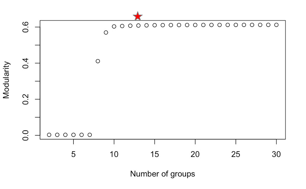
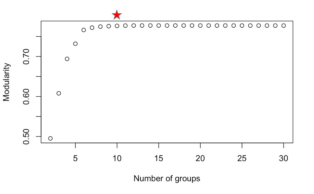
We first choose the number of groups $G$. Figure 6(a) shows the modularity value under different values of $G$. As one can see, the modularity value reaches its peak when $G=13$ and then remains almost the same as $G$ further increases. Therefore, we divide the network into $G=13$ groups.

Figure 4 shows the seven largest identified groups, where different colors correspond to different estimated groups. Roughly speaking, these seven groups represent seven different regions in the world. For example, the black points are mainly in South America, the pink points are mainly in Canada, while the yellow points are mainly in the United States, Mexico, and the Caribbean region.

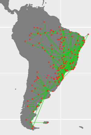
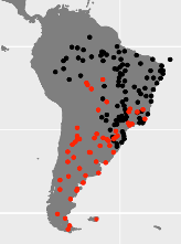
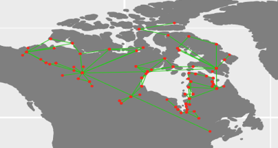
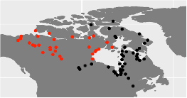
Community detection is then applied to each identified group. For example, the right panel of Figure 5(a) shows the community detection results for the group in South America. As one can see, the two detected communities correspond to the two centers in the left panel of Figure 5(a): one in Uruguay and Argentina, and the other in Brazil, which are understandable. Another example is shown in Figure 5(b). Two detected communities (lower panel) match the airline routes in the upper panel and correspond to eastern and western Canada, respectively.

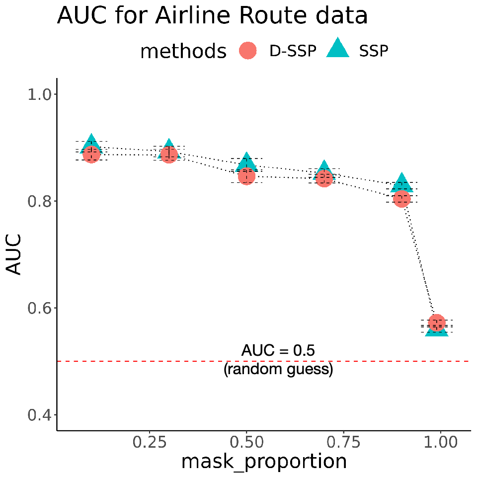
Further, we evaluate the effectiveness of community detection in a predictive manner. Specifically, we first randomly sample a proportion of the node pairs as the testing set and mask the corresponding edge $A_{ij}$ values as zero; then we apply the proposed community detection method to obtain $\hat{{\bm{\mathbf{B}}}}_{n}$ which can be estimated according to the detected community labels $\hat{{\bm{\mathbf{c}}}}$ by considering the connection probability of nodes both within and between communities. Lastly, we evaluate the performance of $\hat{{\bm{\mathbf{B}}}}_{n}$ on the testing set using the area under the receiver operating characteristic curve (AUC). The left panel in Figure 7 shows how the AUC value changes when we vary the proportion of masked node pairs. As we can see, overall, the AUC values are pretty high and stable. As the proportion of masked node pairs increases, the AUC value decreases, but not by a lot. We can also see that the AUC of D-SSP is only slightly lower than that of SSP, indicating again that with data splitting, the proposed distributed community detection method does not degrade the community detection performance.

(a) Airline route network

(b) Facebook ego network

Figure 6: Modularity under different values of $G$

6.2 Ego Networks

Ego networks (Leskovec and Mcauley, 2012; Leskovec and Krevl, 2014) are often created from user surveys in social media, such as Facebook, Twitter, or Google$+$. Each ego person is considered as a primary node, and the ego’s friends are all considered as nodes in the ego network. If two nodes in the ego network are friends with each other, a link is added between these two nodes. For example, the Facebook ego network we consider here contains 4,039 nodes and 88,234 edges, corresponding to 10 ego people (see Figure 8).

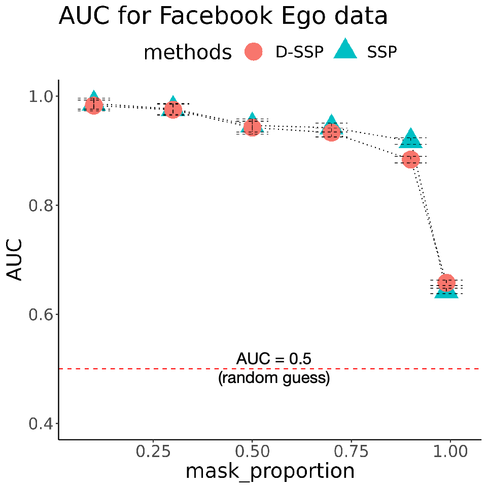
Since there are 10 ego people in this Facebook ego network, it is reasonable to set the number of groups $G$ as 10. The plot of modularity for the ego network (Figure 6(b)), which shows the modularity value under different values of $G$, confirms the conjecture. As one can see, the modularity value reaches its peak at $G=10$ and stays at about the same value for large $G$ values. After setting the number of groups as 10, we apply the D-SSP method to the Facebook ego network to obtain the estimated community labels and link probability matrix. Similar to the previous subsection, the results are evaluated using the AUC on the testing set (see Figure 7).

Figure 7: AUC under different proportions of masked node pairs. The x-axis for masked proportion is set as 0.1, 0.3, 0.5, 0.7, 0.99 respectively.

Network	Egos	Nodes	Edges	AUC (mask $10\%$) (D-SSP)	Time (D-SSP)	AUC (mask $10\%$) (SSP)	Time (SSP)
Facebook	10	4,039	88,234	0.985	44(s)	0.986	214(s)
Twitter	42	5,816	83,694	0.991	34(s)	0.989	420(s)
Google$+$	8	6,382	325,819	0.941	101(s)	0.954	761(s)
Twitter	142	81,306	1,342,296	0.989	1091(s)	——	——
Google$+$	132	107,614	13,673,453	0.974	5030(s)	——	——

Table 2: Numerical results for ego networks; all experiments are conducted via a Dell R7425 machine with dual processor AMD Epyc 32 core 2.2 GHZ with 8GB of RAM

Further, we have also considered a Twitter ego network and a Google$+$ ego network. Since these two networks are relatively large (with 142 and 132 ego people respectively), the SSP method can not be applied due to the computational cost. We thus apply the SSP method only on a subset of the ego network corresponding to a randomly sampled subset of the ego people. The results are shown in Table 2. It can be seen that the proposed distributed community detection method D-SSP has comparable performance to SSP (when SSP can be applied) in terms of the AUC, but significantly reducing the computational cost.

7 Conclusion and Future Work

In this paper, we have proposed a novel distributed community detection method for large networks with a grouped community structure. The method is easy to implement using the current technology in modularity optimization and community detection. We have also established both weak and strong consistency of the proposed method for both group and community detection. Numerical results show that the proposed distributed community detection method achieves similar detection performance in comparison to community detection methods without data splitting, but largely reduces the computational cost.

There are several directions we plan to extend our work. The number of groups $G$ is currently assumed fixed as $n$ grows in our theoretical analysis. Using techniques developed in Choi et al. (2012) and Rohe et al. (2011), we may relax this assumption. Another interesting direction is to generalize the current work to incorporate the dynamic representation of time-varying networks with evolving community structures (Sarkar and Moore, 2006; Berger-Wolf and Saia, 2006). This is challenging and requires further investigation.

Appendix

We first formally formulate the group detection problem for networks with the grouped community structure. Given the total number of groups $G$, we use ${\bm{\mathbf{e}}}$ to denote a group assignment ${\bm{\mathbf{e}}}=\{e_{1},e_{2},\ldots,e_{n}\}$, where $e_{i}$ is the group label for node $v_{i}$ and it takes value in $\{1,2,\ldots,G\}$. Define $\hat{{\bm{\mathbf{g}}}}=\mbox{argmax}_{{\bm{\mathbf{e}}}}{Q_{ER}({\bm{\mathbf{e}}})}$ as the estimated group labels. Our first goal is to show that $\hat{{\bm{\mathbf{g}}}}$ can consistently estimate the true group labels ${\bm{\mathbf{g}}}$. Following Bickel and Chen (2009) and Zhao et al. (2012), for any given group assignment ${\bm{\mathbf{e}}}$, we construct matrix ${\bm{\mathbf{O}}}({\bm{\mathbf{e}}})\in\mathbb{R}^{G\times G}$ as

$$O_{ts}({\bm{\mathbf{e}}})=\sum_{ij}A_{ij}I\{e_{i}=t,e_{j}=s\},$$

where $I$ is the indicator function. The total degree in group $t$ under the group assignment ${\bm{\mathbf{e}}}$ can be defined as

$$O_{t}({\bm{\mathbf{e}}})=\sum_{s}O_{ts}({\bm{\mathbf{e}}}),\qquad t=1,\dots,G.$$

Let ${\bm{\mathbf{f}}}({\bm{\mathbf{e}}})=(\frac{n_{1}(e)}{n},\frac{n_{2}(e)}{n},...,\frac{n_{G}(e)}{n})^{T}$ denote the frequencies in each group under the group assignment ${\bm{\mathbf{e}}}$, where $n_{t}({\bm{\mathbf{e}}})=\sum_{i}I\{e_{i}=t\}$ is the number of nodes in group $t$. Also, denote the sum of degrees as $L=\sum_{ij}A_{ij}$.

We start with the general format of modularity-based criteria, which can be written as

$$Q({\bm{\mathbf{e}}})=F(\frac{{\bm{\mathbf{O}}}({\bm{\mathbf{e}}})}{\mu_{n}},{\bm{\mathbf{f}}}({\bm{\mathbf{e}}})).$$

We aim to find an e that maximizes the modularity.

The key in group detection problem is to construct a “population version” of $Q({\bm{\mathbf{e}}})$ such that the group labels ${\bm{\mathbf{g}}}$ can maximize the “population version” of $Q({\bm{\mathbf{e}}})$. We first need to construct the “population version” of ${\bm{\mathbf{f}}}({\bm{\mathbf{e}}})$ and $O({\bm{\mathbf{e}}})$.

We define a matrix ${\bm{\mathbf{R}}}({\bm{\mathbf{e}}})\in\mathbb{R}^{G\times K\times M}$ as $R_{tau}({\bm{\mathbf{e}}})=\frac{1}{n}\sum_{i}I(e_{i}=t,c_{i}=a,\theta_{i}=x_{u})$, which is a normalized one-hot representation of the relationship between nodes and structure including group label, community labels and degree level. For any generic array ${\bm{\mathbf{S}}}=[S_{tau}]\in\mathbb{R}^{G\times K\times M}$, we can define a G-dimensional vector ${\bm{\mathbf{h}}}({\bm{\mathbf{S}}})=[h_{t}({\bm{\mathbf{S}}})]$ by

$$h_{t}({\bm{\mathbf{S}}})=\sum_{au}S_{tau},$$ (4)

and $G\times G$ matrix ${\bm{\mathbf{H}}}({\bm{\mathbf{S}}})=[H_{ts}({\bm{\mathbf{S}}})]$ by

$$H_{ts}({\bm{\mathbf{S}}})=\sum_{abuv}x_{u}x_{v}B_{ab}S_{ta}S_{sb}.$$ (5)

Then we have Lemma 3 as follows:

Lemma 3.

$$E(f_{t}({\bm{\mathbf{e}}})|{\bm{\mathbf{c}}},{\bm{\mathbf{\theta}}})=h_{t}({\bm{\mathbf{R}}}({\bm{\mathbf{e}}})),$$

$$\frac{1}{u_{n}}E(O_{ts}({\bm{\mathbf{e}}})|{\bm{\mathbf{c}}},{\bm{\mathbf{\theta}}})=H_{ts}({\bm{\mathbf{R}}}({\bm{\mathbf{e}}})).$$

Proof of Lemma 3: For the first equation, left part can be written as $E(f_{t}({\bm{\mathbf{e}}})|{\bm{\mathbf{c}}},{\bm{\mathbf{\theta}}})=f_{t}({\bm{\mathbf{e}}})=\frac{1}{n}\sum_{i}I(e_{i}=t)$ due to the definition of $f_{t}({\bm{\mathbf{e}}})$. From the construction of ${\bm{\mathbf{h}}}$ and ${\bm{\mathbf{R}}}({\bm{\mathbf{e}}})$ above, we have $h_{t}({\bm{\mathbf{R}}}({\bm{\mathbf{e}}}))=\sum_{au}R_{tau}({\bm{\mathbf{e}}})=\sum_{au}\frac{1}{n}\sum_{i}I(e_{i}=t,c_{i}=a,\theta_{i}=x_{u})$. After changing the order of two summations, we have

$$\sum_{au}\frac{1}{n}\sum_{i}I(e_{i}=t,c_{i}=a,\theta_{i}=x_{u})=\sum_{i}\frac{1}{n}\sum_{au}I(e_{i}=t,c_{i}=a,\theta_{i}=x_{u})=\frac{1}{n}\sum_{i}I(e_{i}=t).$$

The last equality holds because community labels ${\bm{\mathbf{c}}}$ and degrees ${\bm{\mathbf{\theta}}}$ take exact one value for each $i$. Therefore, $E(f_{t}({\bm{\mathbf{e}}})|{\bm{\mathbf{c}}},{\bm{\mathbf{\theta}}})=h_{t}({\bm{\mathbf{R}}}({\bm{\mathbf{e}}}))$.

For the second equation, we have by definition of $O_{ts}$:

$$\begin{split}\frac{1}{u_{n}}E(O_{ts}({\bm{\mathbf{e}}})|{\bm{\mathbf{c}}},{\bm{\mathbf{\theta}}})&=\frac{1}{u_{n}}E(\sum_{ij}A_{ij}{I\{e_{i}=t,e_{j}=s\}}|{\bm{\mathbf{c}}},{\bm{\mathbf{\theta}}})\\ &=\frac{1}{u_{n}}E(\sum_{ij}\sum_{abuv}A_{ij}I\{e_{i}=t,g_{i}=a,\theta_{i}=x_{u}\}I\{e_{j}=s,g_{j}=b,\theta_{j}=x_{v}\}|{\bm{\mathbf{c}}},{\bm{\mathbf{\theta}}}).\end{split}$$

Given community labels and degrees, the adjacency matrix ${\bm{\mathbf{A}}}$ is constructed from the probability matrix ${\bm{\mathbf{B}}}_{n}=\rho_{n}{\bm{\mathbf{B}}}$. Therefore, we have:

$$\begin{split}&\frac{1}{u_{n}}E(\sum_{ij}\sum_{abuv}A_{ij}I\{e_{i}=t,g_{i}=a,\theta_{i}=x_{u}\}I\{e_{j}=s,g_{j}=b,\theta_{j}=x_{v}\}|{\bm{\mathbf{c}}},{\bm{\mathbf{\theta}}})\\ &=\frac{\rho_{n}}{u_{n}}\sum_{ij}\theta_{i}\theta_{j}B_{c_{i},c_{j}}\sum_{abuv}I\{e_{i}=t,g_{i}=a,\theta_{i}=x_{u}\}I\{e_{j}=s,g_{j}=b,\theta_{j}=x_{v}\}\\ &=\frac{1}{n^{2}}\sum_{abuv}x_{u}x_{v}B_{ab}\sum_{ij}I\{e_{i}=t,g_{i}=a,\theta_{i}=x_{u}\}I\{e_{j}=s,g_{j}=b,\theta_{j}=x_{v}\}.\end{split}$$

From the construction of ${\bm{\mathbf{H}}}$ and ${\bm{\mathbf{R}}}({\bm{\mathbf{e}}})$, the following equations holds:

$$\begin{split}H_{ts}({\bm{\mathbf{R}}}({\bm{\mathbf{e}}}))&=\frac{1}{n^{2}}\sum_{abuv}x_{u}x_{v}B_{ab}R_{ta}({\bm{\mathbf{e}}})R_{sb}({\bm{\mathbf{e}}})\\ &=\sum_{ab}x_{u}x_{v}B_{ab}\sum_{i}I(e_{i}=t,c_{i}=a)\sum_{j}I(e_{j}=s,c_{j}=b).\end{split}$$

Therefore, $\frac{1}{u_{n}}E(O_{ts}({\bm{\mathbf{e}}})|{\bm{\mathbf{c}}})=H_{ts}({\bm{\mathbf{R}}}({\bm{\mathbf{e}}})).$  

From the Lemma 3, the “population version” of $Q({\bm{\mathbf{e}}})$ can be defined as the expectation conditional on ${\bm{\mathbf{c}}}$ but replacing ${\bm{\mathbf{R}}}({\bm{\mathbf{e}}})$ by ${\bm{\mathbf{T}}}({\bm{\mathbf{e}}})\in\mathbb{R}^{G\times K\times M}$, where

$$T_{tau}({\bm{\mathbf{e}}})=\frac{\sum_{i}I(e_{i}=t,c_{i}=a,\theta_{i}=x_{u})}{\sum_{i}I(c_{i}=a,\theta_{i}=x_{u})}\tau_{au},$$

it can be shown that $T_{tau}({\bm{\mathbf{e}}})=R_{tau}({\bm{\mathbf{e}}})\tau_{au}/\hat{\tau}_{au}$, where $\tau_{au}=\mathbb{P}(c_{i}=a,\theta_{i}=x_{u})$ and $\hat{\tau}_{au}=\frac{1}{n}\sum_{i}I(c_{i}=a,\theta_{i}=x_{u})$. Therefore, the “population version” of $Q({\bm{\mathbf{e}}})$ can be further denoted as $F({\bm{\mathbf{H}}}({\bm{\mathbf{T}}}({\bm{\mathbf{e}}})),{\bm{\mathbf{h}}}({\bm{\mathbf{T}}}({\bm{\mathbf{e}}})))$, where we omit the constant multiplier $L$. Theorem 1 would indicate that the group labels g are the maximizer of $F({\bm{\mathbf{H}}}({\bm{\mathbf{T}}}({\bm{\mathbf{e}}})),{\bm{\mathbf{h}}}({\bm{\mathbf{T}}}({\bm{\mathbf{e}}})))$.

Lemma 4 is based on Bernstein’s inequality which is utilized in Lemma 5. Lemma 5 provides the conditions for the consistency in maximizing modularity $Q({\bm{\mathbf{e}}})$.

Lemma 4.

Define ${\bm{\mathbf{X}}}({\bm{\mathbf{e}}})\in\mathbb{R}^{G\times G}$ by $X_{ts}({\bm{\mathbf{e}}})=\frac{{\bm{\mathbf{O}}}({\bm{\mathbf{e}}})}{\mu_{n}}-{\bm{\mathbf{H}}}({\bm{\mathbf{R}}}({\bm{\mathbf{e}}}))$. Let $||{\bm{\mathbf{X}}}||=max_{s,t}|X_{st}|$ and $|{\bm{\mathbf{e}}}-{\bm{\mathbf{g}}}|=\sum_{i}I(e_{i}\neq g_{i})$. Then

$$P(max_{{\bm{\mathbf{e}}}}||{\bm{\mathbf{X}}}({\bm{\mathbf{e}}})||_{\infty}\geq\varepsilon)\leq 2G^{n+2}exp(-\frac{1}{8C}\varepsilon^{2}\mu_{n})$$ (6)

for $\varepsilon<3C$, where $C=max_{ab}B_{ab}$.

$$P(max_{|{\bm{\mathbf{e}}}-{\bm{\mathbf{g}}}|\leq m}||{\bm{\mathbf{X}}}({\bm{\mathbf{e}}})-{\bm{\mathbf{X}}}({\bm{\mathbf{g}}})||_{\infty}\geq\varepsilon)\leq 2\binom{n}{m}G^{m+2}exp(-\frac{3}{8}\varepsilon\mu_{n})$$ (7)

for $\varepsilon\geq 6Cm/n$.

$$P(max_{|{\bm{\mathbf{e}}}-{\bm{\mathbf{g}}}|\leq m}||{\bm{\mathbf{X}}}({\bm{\mathbf{e}}})-{\bm{\mathbf{X}}}({\bm{\mathbf{g}}})||_{\infty}\geq\varepsilon)\leq 2\binom{n}{m}G^{m+2}exp(-\frac{n}{16C}\varepsilon^{2}\mu_{n})$$ (8)

for $\varepsilon\leq 6Cm/n$.

Proof: See the proof of Lemma A.1. in the supplementary material of Zhao et al. (2012).  

Lemma 5.

For any $Q({\bm{\mathbf{e}}})$ of the form

$$Q({\bm{\mathbf{e}}})=F(\frac{{\bm{\mathbf{O}}}({\bm{\mathbf{e}}})}{\mu_{n}},{\bm{\mathbf{f}}}({\bm{\mathbf{e}}}))$$

if ${\bm{\mathbf{\pi}}},{\bm{\mathbf{B}}},F$ satisfy conditions (*), (a),(b),(c), then Q is strongly consistent under stochastic block models if $\lambda_{n}/(log(n))\rightarrow\infty$ and weakly consistent when $\lambda_{n}\rightarrow\infty.$

The conditions are listed as follows:

(*) $F({\bm{\mathbf{H}}}({\bm{\mathbf{S}}}),{\bm{\mathbf{h}}}({\bm{\mathbf{S}}}))$ is uniquely maximized over $\mathscr{P}=\{{\bm{\mathbf{S}}}:{\bm{\mathbf{S}}}\geq 0,\sum_{t=1}^{G}S_{tau}=\tau_{au}\}$ by ${\bm{\mathbf{S}}}={\bm{\mathbf{S}}}^{*}$, where ${\bm{\mathbf{S}}}^{*}_{tau}=\tau_{au}$ for one $t$, otherwise, ${\bm{\mathbf{S}}}^{*}_{t^{\prime}au}=0$ for $t^{\prime}\neq t$. ${\bm{\mathbf{S}}}^{*}_{\cdot\cdot u}$ has only one nonzero element in each column, and communities within group stay in the same row.

(a) $F$ is Lipschitz in its arguments;

(b) Let ${\bm{\mathbf{W}}}={\bm{\mathbf{H}}}({\bm{\mathbf{D}}})$. The directional derivatives $\frac{\partial^{2}F}{\partial\varepsilon^{2}}({\bm{\mathbf{M}}}_{0}+\varepsilon({\bm{\mathbf{M}}}_{1}-{\bm{\mathbf{M}}}_{0}),{\bm{\mathbf{t}}}_{0}+\varepsilon({\bm{\mathbf{t}}}_{1}-{\bm{\mathbf{t}}}_{0}))|_{\varepsilon=0+}$ are continuous in $({\bm{\mathbf{M}}}_{1},{\bm{\mathbf{t}}}_{1})$ for all $({\bm{\mathbf{M}}}_{0},{\bm{\mathbf{t}}}_{0})$ in a neighborhood of $({\bm{\mathbf{W}}},{\bm{\mathbf{\pi}}})$;

(c) Let $G({\bm{\mathbf{S}}})=F({\bm{\mathbf{H}}}({\bm{\mathbf{S}}}),{\bm{\mathbf{h}}}({\bm{\mathbf{S}}}))$. Then on $\mathscr{P}$, $\frac{\partial G((1-\varepsilon){\bm{\mathbf{D}}}+\varepsilon{\bm{\mathbf{S}}})}{\partial\varepsilon}|_{\varepsilon=0+}<-C<0$ for all ${\bm{\mathbf{\pi}}},{\bm{\mathbf{B}}}$.

Proof:

The proof has three steps.

Step 1: show that the modularity $Q({\bm{\mathbf{e}}})=F(\frac{{\bm{\mathbf{O}}}({\bm{\mathbf{e}}})}{\mu_{n}},{\bm{\mathbf{f}}}({\bm{\mathbf{e}}}))$ is uniformly close to the population version $F({\bm{\mathbf{H}}}({\bm{\mathbf{T}}}({\bm{\mathbf{e}}})),{\bm{\mathbf{h}}}({\bm{\mathbf{T}}}({\bm{\mathbf{e}}})))$. In another word, we need to show that for $\lambda_{n}\rightarrow\infty$, there exist $\varepsilon_{n}\rightarrow 0$ such that

$$P(max_{{\bm{\mathbf{e}}}}|F(\frac{{\bm{\mathbf{O}}}({\bm{\mathbf{e}}})}{\mu_{n}},{\bm{\mathbf{f}}}({\bm{\mathbf{e}}}))-F({\bm{\mathbf{H}}}({\bm{\mathbf{T}}}({\bm{\mathbf{e}}})),{\bm{\mathbf{h}}}({\bm{\mathbf{T}}}({\bm{\mathbf{e}}})))|<\varepsilon_{n})\rightarrow 1.$$ (9)

Since

$$\begin{split}&|F(\frac{{\bm{\mathbf{O}}}({\bm{\mathbf{e}}})}{\mu_{n}},{\bm{\mathbf{f}}}({\bm{\mathbf{e}}}))-F({\bm{\mathbf{H}}}({\bm{\mathbf{T}}}({\bm{\mathbf{e}}})),{\bm{\mathbf{h}}}({\bm{\mathbf{T}}}({\bm{\mathbf{e}}})))|\\ &\leq|F(\frac{{\bm{\mathbf{O}}}({\bm{\mathbf{e}}})}{\mu_{n}},{\bm{\mathbf{f}}}({\bm{\mathbf{e}}}))-F({\bm{\mathbf{H}}}({\bm{\mathbf{R}}}({\bm{\mathbf{e}}})),{\bm{\mathbf{h}}}({\bm{\mathbf{R}}}({\bm{\mathbf{e}}})))|+|F({\bm{\mathbf{H}}}({\bm{\mathbf{R}}}({\bm{\mathbf{e}}})),{\bm{\mathbf{h}}}({\bm{\mathbf{R}}}({\bm{\mathbf{e}}})))-F({\bm{\mathbf{H}}}({\bm{\mathbf{T}}}({\bm{\mathbf{e}}})),{\bm{\mathbf{h}}}({\bm{\mathbf{T}}}({\bm{\mathbf{e}}})))|,\end{split}$$

For the first item on the left hand above, since ${\bm{\mathbf{h}}}({\bm{\mathbf{R}}}({\bm{\mathbf{e}}}))=f({\bm{\mathbf{e}}})$ and by Lipschitz continuity,

$$|F(\frac{{\bm{\mathbf{O}}}({\bm{\mathbf{e}}})}{\mu_{n}},{\bm{\mathbf{f}}}({\bm{\mathbf{e}}}))-F({\bm{\mathbf{H}}}({\bm{\mathbf{R}}}({\bm{\mathbf{e}}})),{\bm{\mathbf{f}}}({\bm{\mathbf{e}}}))|\leq M_{1}||{\bm{\mathbf{X}}}({\bm{\mathbf{e}}})||_{\infty}.$$ (10)

From Equation 6 in Lemma 4, Equation 10 tends to 0 uniformly for $\lambda_{n}\rightarrow\infty$. For the second item,

$$\begin{split}&|F({\bm{\mathbf{H}}}({\bm{\mathbf{R}}}({\bm{\mathbf{e}}})),{\bm{\mathbf{f}}}({\bm{\mathbf{e}}}))-F({\bm{\mathbf{H}}}({\bm{\mathbf{T}}}({\bm{\mathbf{e}}})),{\bm{\mathbf{h}}}({\bm{\mathbf{T}}}({\bm{\mathbf{e}}})))|\\ &\leq M_{1}||{\bm{\mathbf{H}}}({\bm{\mathbf{R}}}({\bm{\mathbf{e}}}))-{\bm{\mathbf{h}}}({\bm{\mathbf{T}}}({\bm{\mathbf{e}}}))||_{\infty}+M_{2}||{\bm{\mathbf{H}}}({\bm{\mathbf{R}}}({\bm{\mathbf{e}}}))-{\bm{\mathbf{h}}}({\bm{\mathbf{T}}}({\bm{\mathbf{e}}}))||_{2},\end{split}$$ (11)

where $||.||_{2}$ is Euclidean norm for vectors. Since for $\lambda_{n}\rightarrow\infty$, $R_{ta}({\bm{\mathbf{e}}})\rightarrow T_{ta}({\bm{\mathbf{e}}})\ \ a.s.$, Equation 11 converges to 0 uniformly too. Thus, Equation 9 holds.

Step 2: show that the weak consistency of group assignments holds. Since ${\bm{\mathbf{T}}}({\bm{\mathbf{g}}})\in\mathscr{P}$ and has only one nonzero element in each column. By continuity and condition $(*)$, there exists $\delta_{n}\rightarrow 0$, if $|{\bm{\mathbf{e}}}-{\bm{\mathbf{g}}}|/n=\sum_{i}I(e_{i}\neq g_{i})/n\geq\delta_{n}$, then

$$F({\bm{\mathbf{H}}}({\bm{\mathbf{T}}}({\bm{\mathbf{g}}})),{\bm{\mathbf{h}}}({\bm{\mathbf{T}}}({\bm{\mathbf{g}}})))-F({\bm{\mathbf{H}}}({\bm{\mathbf{T}}}({\bm{\mathbf{e}}})),{\bm{\mathbf{h}}}({\bm{\mathbf{T}}}({\bm{\mathbf{e}}})))>2\varepsilon_{n}.$$

From Equation 9 in step 1, it is can be shown that

$$\begin{split}&P(max_{\{{\bm{\mathbf{e}}}:|{\bm{\mathbf{e}}}-{\bm{\mathbf{g}}}|/n\geq\delta_{n}\}}F(\frac{{\bm{\mathbf{O}}}({\bm{\mathbf{e}}})}{\mu_{n}},{\bm{\mathbf{f}}}({\bm{\mathbf{e}}}))<F(\frac{{\bm{\mathbf{O}}}({\bm{\mathbf{g}}})}{\mu_{n}},{\bm{\mathbf{f}}}({\bm{\mathbf{g}}})))\\ &\geq P(|max_{\{{\bm{\mathbf{e}}}:|{\bm{\mathbf{e}}}-{\bm{\mathbf{g}}}|/n\geq\delta_{n}\}}F(\frac{{\bm{\mathbf{O}}}({\bm{\mathbf{e}}})}{\mu_{n}},{\bm{\mathbf{f}}}({\bm{\mathbf{e}}}))-max_{\{{\bm{\mathbf{e}}}:|{\bm{\mathbf{e}}}-{\bm{\mathbf{g}}}|/n\geq\delta_{n}\}}F({\bm{\mathbf{H}}}({\bm{\mathbf{T}}}({\bm{\mathbf{e}}})),{\bm{\mathbf{h}}}({\bm{\mathbf{T}}}({\bm{\mathbf{e}}})))|<\varepsilon_{n},\\ &|F(\frac{{\bm{\mathbf{O}}}({\bm{\mathbf{g}}})}{\mu_{n}},{\bm{\mathbf{f}}}({\bm{\mathbf{g}}}))-F({\bm{\mathbf{H}}}({\bm{\mathbf{T}}}({\bm{\mathbf{e}}})),{\bm{\mathbf{h}}}({\bm{\mathbf{T}}}({\bm{\mathbf{e}}})))|<\varepsilon_{n})\rightarrow 1\end{split}$$ (12)

The Equation 12 implies that $P(|{\bm{\mathbf{e}}}-{\bm{\mathbf{g}}}|/n<\delta_{n})\rightarrow 1$, and weak consistency of group assignment holds.

Step 3: show that the strong consistency of group assignments holds. See the step 3 of the proof of of Theorem 4.1 in the Zhao et al. (2012).  

Now we provide the proof of Theorem 1.

Proof of Theorem 1:

Under the block assumption $\theta_{i}\equiv 1$, the population version of $Q_{ER}({\bm{\mathbf{e}}})$ is $F({\bm{\mathbf{H}}}({\bm{\mathbf{S}}}),{\bm{\mathbf{h}}}({\bm{\mathbf{S}}}))=\sum_{t}(H_{tt}({\bm{\mathbf{S}}})-B_{0}h_{t}^{2}({\bm{\mathbf{S}}}))$ up to a constant multiplier, where ${\bm{\mathbf{S}}}\in\mathbb{R}^{G\times K}$. Therefore, it satisfies conditions (a),(b),(c) and we only need to show condition (*) is satisfied as well.

For ${\bm{\mathbf{S}}}\in\mathscr{P}$, we have the following equation:

$$\begin{split}&\sum^{G}_{t}(H_{tt}({\bm{\mathbf{S}}})-B_{0}h^{2}_{t}({\bm{\mathbf{S}}}))+\sum^{G}_{t\neq s}(H_{ts}({\bm{\mathbf{S}}})-B_{0}h_{t}({\bm{\mathbf{S}}})h_{s}({\bm{\mathbf{S}}}))\\ &=\sum^{G}_{t,s}H_{ts}({\bm{\mathbf{S}}})-B_{0}(\sum^{G}_{t}h_{t}({\bm{\mathbf{S}}}))^{2}\\ &=1-1^{2}=0.\end{split}$$ (13)

The second last equality holds due to Lemma 3 and the fact that $\sum_{t}f_{t}=1$ and $\frac{\sum_{ts}O_{ts}}{L}=1$. Also, we construct ${\bm{\mathbf{\Delta}}}\in\mathbb{R}^{G\times G}$ by:

$$\Delta_{ts}=(I(t=s)-1/2)\times 2.$$ (14)

From Equation 13 and 14, the population version $F({\bm{\mathbf{H}}}({\bm{\mathbf{S}}}),{\bm{\mathbf{h}}}({\bm{\mathbf{S}}}))$ can be rewritten as:

$$\begin{split}F({\bm{\mathbf{H}}}({\bm{\mathbf{S}}}),{\bm{\mathbf{h}}}({\bm{\mathbf{S}}}))&=\sum^{G}_{t}(H_{tt}({\bm{\mathbf{S}}})-B_{0}h_{t}^{2}({\bm{\mathbf{S}}}))\\ &=\frac{1}{2}\sum^{G}_{t,s}\Delta_{ts}(H_{ts}({\bm{\mathbf{S}}})-B_{0}h_{t}({\bm{\mathbf{S}}})h_{s}({\bm{\mathbf{S}}})).\end{split}$$

From the Definition of $h$ and $H$ in equation 4 and 5, we get:

$$\begin{split}&\frac{1}{2}\sum^{G}_{t,s}\Delta_{ts}(H_{ts}({\bm{\mathbf{S}}})-B_{0}h_{t}({\bm{\mathbf{S}}})h_{s}({\bm{\mathbf{S}}}))\\ =&\frac{1}{2}\sum^{G}_{t,s}\Delta_{ts}(\sum^{K}_{a,b}B_{ab}S_{ta}S_{sb}-B_{0}\sum^{K}_{a}S_{ta}\sum^{K}_{b}S_{sb})\\ =&\frac{1}{2}\sum^{G}_{t,s}\sum^{K}_{a,b}S_{ta}S_{sb}\Delta_{ts}(B_{ab}-B_{0}).\end{split}$$

Construct ${\bm{\mathbf{\Delta}}}^{{\bm{\mathbf{c}}}}\in\mathbb{R}^{K\times K}$ by:

$$\Delta^{{\bm{\mathbf{c}}}}_{ab}=\begin{cases}1,community\ a,\ b\ belong\ to\ same\ group\\ -1,O.W.\end{cases}$$

From the conditions in Condition 1, the following inequality always holds for any $t,s,a,b$:

$$\Delta_{ts}(B_{ab}-B_{0})\leq\Delta^{{\bm{\mathbf{c}}}}_{ab}(B_{ab}-B_{0}).$$

Therefore, population version of modularity satisfies:

$$\begin{split}F({\bm{\mathbf{H}}}({\bm{\mathbf{S}}}),{\bm{\mathbf{h}}}({\bm{\mathbf{S}}}))&=\frac{1}{2}\sum^{G}_{t,s}\sum^{K}_{a,b}S_{ta}S_{sb}\Delta_{ts}(B_{ab}-B_{0})\\ &\leq\frac{1}{2}\sum^{G}_{t,s}\sum^{K}_{a,b}S_{ta}S_{sb}\Delta^{{\bm{\mathbf{c}}}}_{ab}(B_{ab}-B_{0}).\end{split}$$

We can change the order of summations in last item above:

$$\begin{split}&\frac{1}{2}\sum^{G}_{t,s}\sum^{K}_{a,b}S_{ta}S_{sb}\Delta^{{\bm{\mathbf{c}}}}_{ab}(B_{ab}-B_{0})=\frac{1}{2}\sum^{K}_{a,b}\Delta^{{\bm{\mathbf{c}}}}_{ab}(B_{ab}-B_{0})\sum^{G}_{t}S_{ta}\sum^{G}_{s}S_{sb}\\ &=\frac{1}{2}\sum^{K}_{a,b}\pi_{a}\pi_{b}\Delta^{{\bm{\mathbf{c}}}}_{ab}(B_{ab}-B_{0})=F({\bm{\mathbf{H}}}({\bm{\mathbf{S}}}^{*}),{\bm{\mathbf{h}}}({\bm{\mathbf{S}}}^{*})).\end{split}$$

The second last equality holds because ${\bm{\mathbf{S}}}\in\mathscr{P}$. Therefore, we have $F({\bm{\mathbf{H}}}({\bm{\mathbf{S}}}),{\bm{\mathbf{h}}}({\bm{\mathbf{S}}}))\leq F({\bm{\mathbf{H}}}({\bm{\mathbf{S}}}^{*}),{\bm{\mathbf{h}}}({\bm{\mathbf{S}}}^{*}))$ (up to row permutation of ${\bm{\mathbf{S}}}^{*}$). Therefore, condition $(*)$ is also satisfied. From the result in Lemma 5, Theorem 1 holds.  

Proof of Theorem 2:

For the degree-corrected model, we follow a similar strategy in Proof of Theorem 1. The population version of $Q_{NGM}$ can be denoted as

$$F(H({\bm{\mathbf{S}}}))=\sum_{t}(\frac{H_{tt}}{\tilde{B_{0}}}-(\frac{H_{t}}{\tilde{B_{0}}})^{2})$$

we need to show condition (*) is satisfied. From equation,

$$\sum_{t}(\frac{H_{tt}}{\tilde{B_{0}}}-(\frac{H_{t}}{\tilde{B_{0}}})^{2})+\sum_{t\neq s}(\frac{H_{ts}}{\tilde{B_{0}}}-\frac{H_{t}H_{s}}{\tilde{B^{2}_{0}}})=\sum_{ts}\frac{H_{ts}}{\tilde{B_{0}}}-(\sum_{t}\frac{H_{t}}{\tilde{B_{0}}})^{2}=0,$$

we can show

$$\begin{split}F(H({\bm{\mathbf{S}}}))=\frac{1}{2}\Delta_{ts}(\frac{H_{ts}}{\tilde{B_{0}}}-(\sum_{t}\frac{H_{t}}{\tilde{B_{0}}})^{2})\end{split}$$ (15)

From the definition of ${\bm{\mathbf{H}}}$ in Equation 5, it can be shown that

$$H_{ts}=\sum_{ab}\tilde{S}_{ta}\tilde{S}_{sb}B_{ab},$$

and

$$H_{t}=\sum_{ac}\tilde{S}_{ta}\tilde{\pi}_{c}B_{ac}$$

where $\tilde{S}_{ta}=\sum_{u}x_{u}S_{tau}$. Hence, we obtain

$$\begin{split}F(H({\bm{\mathbf{S}}}))&=\frac{1}{2}\sum_{ts}\Delta_{ts}(\frac{\sum_{ab}\tilde{S}_{ta}\tilde{S}_{sb}B_{ab}}{\tilde{B_{0}}}-\frac{\sum_{ac}\tilde{S}_{ta}\tilde{\pi}_{c}B_{ac}\sum_{bd}\tilde{S}_{sb}\tilde{\pi}_{d}B_{bd}}{\tilde{B_{0}}^{2}})\\ &=\frac{1}{2}\sum_{ts}\sum_{ab}\tilde{S}_{ta}\tilde{S}_{sb}\Delta_{ts}(\frac{B_{ab}}{\tilde{B_{0}}}-\frac{(\sum_{c}\tilde{\pi}_{c}B_{ac})(\sum_{d}\tilde{\pi}_{d}B_{bd})}{\tilde{B_{0}}^{2}}).\end{split}$$ (16)

From the condition 3, it satisfies that

$$\begin{split}&\frac{1}{2}\sum_{ts}\sum_{ab}\tilde{S}_{ta}\tilde{S}_{sb}\Delta_{ts}(\frac{B_{ab}}{\tilde{B_{0}}}-\frac{(\sum_{c}\tilde{\pi}_{c}B_{ac})(\sum_{d}\tilde{\pi}_{d}B_{bd})}{\tilde{B_{0}}^{2}})\\ \leq&\frac{1}{2}\sum_{ts}\sum_{ab}\tilde{S}_{ta}\tilde{S}_{sb}\Delta_{ab}^{c}(\frac{B_{ab}}{\tilde{B_{0}}}-\frac{(\sum_{c}\tilde{\pi}_{c}B_{ac})(\sum_{d}\tilde{\pi}_{d}B_{bd})}{\tilde{B_{0}}^{2}})\\ =&F(H({\bm{\mathbf{S}}}^{*}))\end{split}$$ (17)

Therefore, condition $(*)$ is satisfied (up to permutation). From the result in Lemma 5, Theorem 2 holds.  

Proof of Theorem 3:

For weak consistency, given any $\varepsilon>0$:

$$P(\frac{1}{n}\sum_{i=1}^{n}1(\hat{c}_{i}\neq c_{i})\geq\varepsilon)=P(\{\frac{1}{n}\sum_{i=1}^{n}1(\hat{c}_{i}\neq c_{i})\geq\varepsilon\},\hat{{\bm{\mathbf{g}}}}={\bm{\mathbf{g}}})+P(\{\frac{1}{n}\sum_{i=1}^{n}1(\hat{c}_{i}\neq c_{i})\geq\varepsilon\},\hat{{\bm{\mathbf{g}}}}\neq{\bm{\mathbf{g}}})$$

The second item $P(\{\frac{1}{n}\sum_{i=1}^{n}1(\hat{c}_{i}\neq c_{i})\geq\varepsilon\},\hat{{\bm{\mathbf{g}}}}\neq{\bm{\mathbf{g}}})$ tends to zero because of the strong consistency of group labels $\hat{{\bm{\mathbf{g}}}}$.

The first item can be bounded by considering the event under each group. I.e, for nodes in group $t$, $\{\frac{1}{n}\sum_{k=1}^{n_{t}}1(\hat{c}^{sub}_{t,k}\neq c^{sub}_{t,k})\geq\varepsilon,\hat{{\bm{\mathbf{g}}}}={\bm{\mathbf{g}}}\}$ can lead to $\{\frac{1}{n}\sum_{i=1}^{n}1(\hat{c}_{i}\neq c_{i})\geq\varepsilon,\hat{{\bm{\mathbf{g}}}}={\bm{\mathbf{g}}}\}$. Therefore, we have:

$$\begin{split}P(\{\frac{1}{n}\sum_{i=1}^{n}1(\hat{c}_{i}\neq c_{i})\geq\varepsilon\},\hat{{\bm{\mathbf{g}}}}={\bm{\mathbf{g}}})&\leq P(\cup_{t=1,2,..,G}\{\frac{1}{n}\sum_{k=1}^{n_{t}}1(\hat{c}^{sub}_{t,k}\neq c^{sub}_{t,k})\geq\varepsilon,\hat{{\bm{\mathbf{g}}}}={\bm{\mathbf{g}}}\})\\ &=P(\cup_{t=1,2,..,G}\{\frac{1}{n_{t}}\sum_{k=1}^{n_{t}}1(\hat{c}^{sub}_{t,k}\neq c^{sub}_{t,k})\geq\frac{\varepsilon}{\pi_{t}},\hat{{\bm{\mathbf{g}}}}={\bm{\mathbf{g}}}\})\\ &\leq\sum_{t=1}^{G}P(\{\frac{1}{n_{t}}\sum_{k=1}^{n_{t}}1(\hat{c}^{sub}_{t,k}\neq c^{sub}_{t,k})\geq\frac{\varepsilon}{\pi_{t}},\hat{{\bm{\mathbf{g}}}}={\bm{\mathbf{g}}}\}).\end{split}$$

The last part tends to zero for each $t$ due to the weak consistency of the community labels $\hat{{\bm{\mathbf{c}}}}^{sub}_{t},t=1,2,...,G$.

For strong consistency:

$$\begin{split}P(\hat{{\bm{\mathbf{c}}}}\neq{\bm{\mathbf{c}}})&=P(\hat{{\bm{\mathbf{g}}}}={\bm{\mathbf{g}}},\hat{{\bm{\mathbf{c}}}}\neq{\bm{\mathbf{c}}})+P(\hat{{\bm{\mathbf{g}}}}\neq{\bm{\mathbf{g}}},\hat{{\bm{\mathbf{c}}}}\neq{\bm{\mathbf{c}}})\\ &\rightarrow 0+0=0.\end{split}$$

The first item goes to zero from the strong consistency of the estimated community labels in each correct group; the second item goes to zero from the strong consistency of the estimated group label.  

Figure 8: The adjacency matrix for the Facebook ego network; in the network, each node denotes a user and each link denotes two users are friends in Facebook. From the adjacency matrix, we can easily observe several groups of friend list.

References

- Amini et al. (2013) Arash A Amini, Aiyou Chen, Peter J Bickel, and Elizaveta Levina. Pseudo-likelihood methods for community detection in large sparse networks. The Annals of Statistics, 41(4):2097–2122, 2013.
- Berger-Wolf and Saia (2006) Tanya Y Berger-Wolf and Jared Saia. A framework for analysis of dynamic social networks. In Proceedings of the 12th ACM SIGKDD international conference on Knowledge discovery and data mining, pages 523–528. ACM, 2006.
- Bickel and Chen (2009) Peter J Bickel and Aiyou Chen. A nonparametric view of network models and newman–girvan and other modularities. Proceedings of the National Academy of Sciences, pages pnas–0907096106, 2009.
- Blondel et al. (2008) Vincent D Blondel, Jean-Loup Guillaume, Renaud Lambiotte, and Etienne Lefebvre. Fast unfolding of communities in large networks. Journal of statistical mechanics: theory and experiment, 2008(10):P10008, 2008.
- Choi et al. (2012) David S Choi, Patrick J Wolfe, and Edoardo M Airoldi. Stochastic blockmodels with a growing number of classes. Biometrika, 99(2):273–284, 2012.
- Clauset et al. (2004) Aaron Clauset, Mark EJ Newman, and Cristopher Moore. Finding community structure in very large networks. Physical review E, 70(6):066111, 2004.
- Daudin et al. (2008) J-J Daudin, Franck Picard, and Stéphane Robin. A mixture model for random graphs. Statistics and computing, 18(2):173–183, 2008.
- Egghe and Rousseau (1990) Leo Egghe and Ronald Rousseau. Introduction to informetrics: Quantitative methods in library, documentation and information science. Elsevier Science Publishers, 1990.
- Fortunato and Barthelemy (2007) Santo Fortunato and Marc Barthelemy. Resolution limit in community detection. Proceedings of the National Academy of Sciences, 104(1):36–41, 2007.
- Fortunato and Hric (2016) Santo Fortunato and Darko Hric. Community detection in networks: A user guide. Physics Reports, 659:1–44, 2016.
- Guimera et al. (2004) Roger Guimera, Marta Sales-Pardo, and Luís A Nunes Amaral. Modularity from fluctuations in random graphs and complex networks. Physical Review E, 70(2):025101, 2004.
- Handcock et al. (2007) Mark S Handcock, Adrian E Raftery, and Jeremy M Tantrum. Model-based clustering for social networks. Journal of the Royal Statistical Society: Series A (Statistics in Society), 170(2):301–354, 2007.
- Holland et al. (1983) Paul W Holland, Kathryn Blackmond Laskey, and Samuel Leinhardt. Stochastic blockmodels: First steps. Social networks, 5(2):109–137, 1983.
- Jin et al. (2015) Jiashun Jin et al. Fast community detection by score. The Annals of Statistics, 43(1):57–89, 2015.
- Karrer and Newman (2011) Brian Karrer and Mark EJ Newman. Stochastic blockmodels and community structure in networks. Physical review E, 83(1):016107, 2011.
- Leskovec and Krevl (2014) Jure Leskovec and Andrej Krevl. SNAP Datasets: Stanford large network dataset collection. http://snap.stanford.edu/data, June 2014.
- Leskovec and Mcauley (2012) Jure Leskovec and Julian J Mcauley. Learning to discover social circles in ego networks. In Advances in neural information processing systems, pages 539–547, 2012.
- Mori and Malik (2003) Greg Mori and Jitendra Malik. Recognizing objects in adversarial clutter: Breaking a visual captcha. In Computer Vision and Pattern Recognition, 2003. Proceedings. 2003 IEEE Computer Society Conference on, volume 1, pages I–I. IEEE, 2003.
- Newman (2006) Mark EJ Newman. Modularity and community structure in networks. Proceedings of the national academy of sciences, 103(23):8577–8582, 2006.
- Newman (2012) Mark EJ Newman. Communities, modules and large-scale structure in networks. Nature physics, 8(1):25, 2012.
- Newman and Girvan (2004) Mark EJ Newman and Michelle Girvan. Finding and evaluating community structure in networks. Physical review E, 69(2):026113, 2004.
- Qin and Rohe (2013) Tai Qin and Karl Rohe. Regularized spectral clustering under the degree-corrected stochastic blockmodel. In Advances in Neural Information Processing Systems, pages 3120–3128, 2013.
- Rohe et al. (2011) Karl Rohe, Sourav Chatterjee, and Bin Yu. Spectral clustering and the high-dimensional stochastic blockmodel. The Annals of Statistics, 39(4):1878–1915, 2011.
- Sarkar and Moore (2006) Purnamrita Sarkar and Andrew W Moore. Dynamic social network analysis using latent space models. In Advances in Neural Information Processing Systems, pages 1145–1152, 2006.
- Snijders and Nowicki (1997) Tom AB Snijders and Krzysztof Nowicki. Estimation and prediction for stochastic blockmodels for graphs with latent block structure. Journal of classification, 14(1):75–100, 1997.
- Von Luxburg et al. (2008) Ulrike Von Luxburg, Mikhail Belkin, and Olivier Bousquet. Consistency of spectral clustering. The Annals of Statistics, pages 555–586, 2008.
- Wang et al. (2020) Jiangzhou Wang, Jingfei Zhang, Binghui Liu, Ji Zhu, and Jianhua Guo. Fast network community detection with profile-pseudo likelihood methods. arXiv preprint arXiv:2011.00647, 2020.
- Wang and Bickel (2017) YX Rachel Wang and Peter J Bickel. Likelihood-based model selection for stochastic block models. The Annals of Statistics, 45(2):500–528, 2017.
- White and Smyth (2005) Scott White and Padhraic Smyth. A spectral clustering approach to finding communities in graphs. In Proceedings of the 2005 SIAM international conference on data mining, pages 274–285. SIAM, 2005.
- Zhao et al. (2011) Yunpeng Zhao, Elizaveta Levina, and Ji Zhu. Community extraction for social networks. Proceedings of the National Academy of Sciences, 2011.
- Zhao et al. (2012) Yunpeng Zhao, Elizaveta Levina, and Ji Zhu. Consistency of community detection in networks under degree-corrected stochastic block models. The Annals of Statistics, 40(4):2266–2292, 2012.