A Mixed Quantization Network for Computationally Efficient Mobile Inverse Tone Mapping

Abstract

Recovering a high dynamic range (HDR) image from a single low dynamic range (LDR) image, namely inverse tone mapping (ITM), is challenging due to the lack of information in over- and under-exposed regions. Current methods focus exclusively on training high performing but computationally inefficient ITM models, which in turn hinder deployment of the ITM models in resource-constrained environments with limited computing power such as edge and mobile device applications.

To this end, we propose combining efficient operations of deep neural networks with a novel mixed quantization scheme to construct a well performing but computationally efficient mixed quantization network (MQN) which can perform single image ITM on mobile platforms. In the ablation studies, we explore the effect of using different attention mechanisms, quantization schemes and loss functions on the performance of MQN in ITM tasks. In the comparative analyses, ITM models trained using MQN perform on par with the state-of-the-art methods on benchmark datasets. MQN models provide up to 10 times improvement on latency and 25 times improvement on memory consumption.

1 Introduction

High dynamic range (HDR) imaging enables capturing, storing, and displaying images and videos that cover the whole range of illuminance values present in natural scenes [Reinhard et al.(2010)Reinhard, Heidrich, Debevec, Pattanaik, Ward, and Myszkowski]. In contrast, low dynamic range (LDR) imaging technologies only work with a reduced range of values limited by their channel bit depth, thus producing results of inferior perceived quality [Akyüz et al.(2007)Akyüz, Fleming, Riecke, Reinhard, and Bülthoff, Hanhart et al.(2014)Hanhart, Korshunov, and Ebrahimi].

In the last two decades, HDR imaging methods have been applied in different fields and sectors, such as digital games [(2020), Akenine-Möller et al.(2019)Akenine-Möller, Haines, and Hoffman] and photography [Debevec and Malik(1997), Gallo et al.(2015)Gallo, Troccoli, Hu, Pulli, and Kautz], among others. Due to the lack of appropriate HDR displays, HDR content was converted to LDR. This operation, called tone mapping (TM) [Mantiuk et al.(2008)Mantiuk, Daly, and Kerofsky, Drago et al.(2003)Drago, Myszkowski, Annen, and Chiba, Reinhard et al.(2002)Reinhard, Stark, Shirley, and Ferwerda], pursues reproduction of images by reducing the tonal values within the images, which leads to loss of details and inevitable appearance changes in the reproduced images [Akyüz et al.(2007)Akyüz, Fleming, Riecke, Reinhard, and Bülthoff, Eilertsen et al.(2016)Eilertsen, Unger, and Mantiuk]. Recently, there has been a substantial increase in production and commercialization of HDR displays. Sustained by new standards, such as HDR10, the number of HDR TV shipped worldwide has leaped by more than a 10x factor between years 2016-2019 [(2020)]. In contrast, most content to be reproduced is still LDR, thus not attaining the reproduction capabilities of HDR displays.

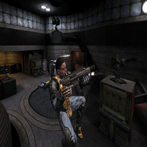
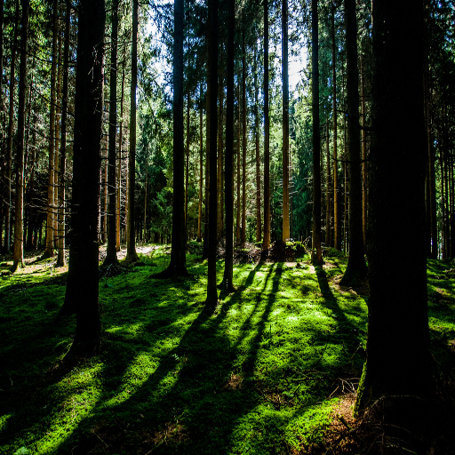
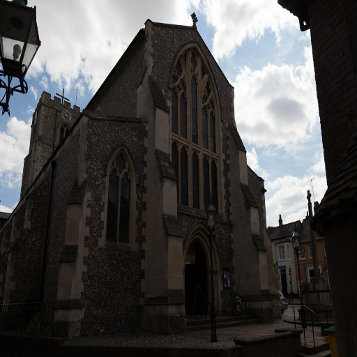
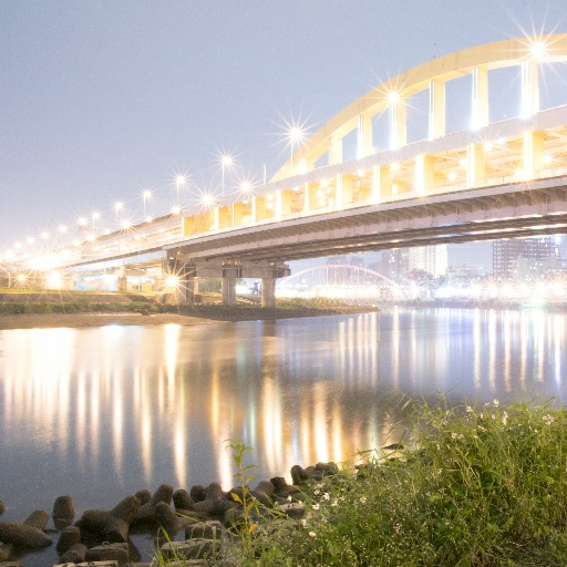
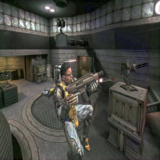
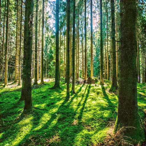
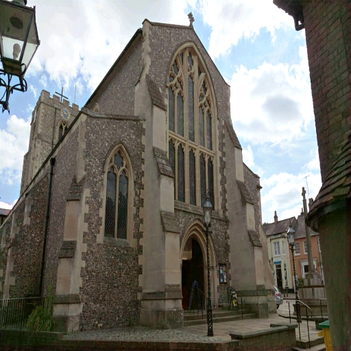
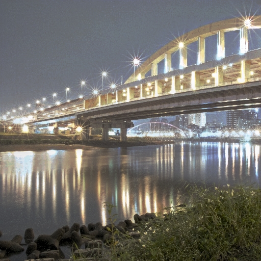
Figure 1: Mobile ITM from single LDR images using mixed quantization network (MQN). Employment of mixed quantization methods and efficient blocks in MQN help reduce computational complexity of HDR image reconstruction (shown at the bottom row) from single LDR images (shown at the top row), and enable its deployment to mobile platforms, achieving a latency of $\approx$21ms on a Samsung Note 20 Exynos 990.

This situation shows the need for the conversion of LDR images into HDR content. This process is referred to as inverse tone mapping (ITM), and involves recreation of the missing information, and expansion and adaptation of the available information to a higher bit depth. Handcrafted ITM algorithms [Banterle et al.(2006)Banterle, Ledda, Debattista, and Chalmers, Rempel et al.(2007)Rempel, Trentacoste, Seetzen, Young, Heidrich, Whitehead, and Ward, Kuo et al.(2012)Kuo, Tang, and Chien, Huo et al.(2014)Huo, Yang, Dong, and Brost, Masia et al.(2009)Masia, Agustin, Fleming, Sorkine, and Gutierrez] focused on range expansion to accommodate the LDR content to the new bit depth, as well as the application of tone operators to linearize the content and adjust the missing information. However, such methods did not provide sufficiently appealing results that could match originally produced HDR content [Banterle et al.(2009)Banterle, Ledda, Debattista, Bloj, Artusi, and Chalmers].

Deep neural networks (DNNs) have been applied to ITM tasks [Serrano et al.(2016)Serrano, Heide, Gutierrez, Wetzstein, and Masia, Eilertsen et al.(2017)Eilertsen, Kronander, Denes, Mantiuk, and Unger, Kim et al.(2020)Kim, Lee, Jo, and Kang] providing state-of-the-art results and products in industrial applications [(2021)]. Nevertheless, current deep-learning-based ITM methods incur high computational costs, both in terms of memory and latency, due to the use of costly operations [Endo et al.(2017)Endo, Kanamori, and Mitani, Marnerides et al.(2018)Marnerides, Bashford-Rogers, Hatchett, and Debattista], large models [Liu et al.(2020)Liu, Lai, Chen, Kao, Yang, Chuang, and Huang, Lee et al.(2018a)Lee, An, and Kang] or feedback loops [Khan et al.(2019)Khan, Khanna, and Raman, Kim et al.(2020)Kim, Lee, Jo, and Kang], among other factors. Such burdens impede their deployment and usage in resource-constrained environments, such as edge devices and mobile phones.

In the present work, we propose a novel Mixed Quantization Network (MQN) for computationally efficient mobile ITM by integrating different quantization schemes applied to models, deploying efficient convolutions into models, and training models using input data. The proposed MQN enables attaining similar accuracy compared to state-of-the-art methods on a reference ITM dataset and can be deployed to a mobile platform to perform more computationally efficient inference. Further, it can be utilised by different hardware platforms, such as CPU or GPU, due to the flexibility of its components and structure. More precisely, our models can perform 10x to 100x times faster inference than competing methods (sample results are given in Figure 1). As far as the authors are aware, this is the first work devoted to constructing computationally efficient DNN-based ITM methods for mobile ITM tasks.

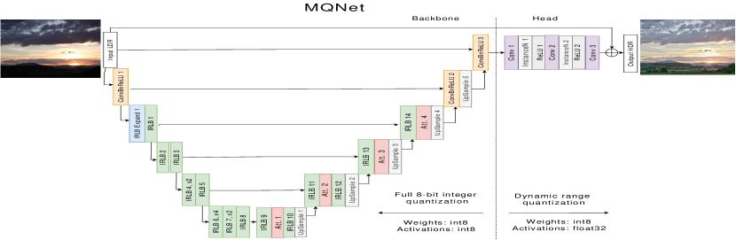
Figure 2: Illustration of the base backbone and high precision head that comprise the MQN. IRLB is used for fast inference and gated attention mechanisms [Zhang et al.(2018)Zhang, Li, Li, Wang, Zhong, and Fu] for improvement of feature representation learning accuracy. The dotted line indicates the separation between the fully quantized architecture and the dynamically quantized head. Input is added to output of the head to produce the overall output. Hyperparameters are given in the supp. mat.

2 Related Work

Vanilla ITM Methods. Vanilla ITM methods have been implemented using tone operators [Banterle et al.(2006)Banterle, Ledda, Debattista, and Chalmers], expansion algorithms [Banterle et al.(2006)Banterle, Ledda, Debattista, and Chalmers, Masia et al.(2017)Masia, Serrano, and Gutierrez, Masia et al.(2009)Masia, Agustin, Fleming, Sorkine, and Gutierrez], such as gamma curve expansion and over-exposed region enhancement [Rempel et al.(2007)Rempel, Trentacoste, Seetzen, Young, Heidrich, Whitehead, and Ward], among other techniques [Akyüz et al.(2007)Akyüz, Fleming, Riecke, Reinhard, and Bülthoff, Huo et al.(2014)Huo, Yang, Dong, and Brost]. A great benefit, in general, of such methods is their low computing power requirement. However, they struggle in generation of high quality image content on over- and under-exposed image regions [Endo et al.(2017)Endo, Kanamori, and Mitani].

DNN-based ITM methods. Recently, DNNs have been employed on ITM tasks. Although most of these methods blatantly differ regarding network architectures and model training components, they can be categorized into three main groups.

The methods in the first group [Zhou et al.(2020)Zhou, Zhao, Han, Xu, Xu, Huang, and Shi, Liu et al.(2020)Liu, Lai, Chen, Kao, Yang, Chuang, and Huang, Khan et al.(2019)Khan, Khanna, and Raman, Marnerides et al.(2018)Marnerides, Bashford-Rogers, Hatchett, and Debattista, Ning et al.(2018)Ning, Xu, Song, Xie, and Zhang, Yang et al.(2018)Yang, Xu, Song, Zhang, Wei, and Lau, Zhang and Lalonde(2017), Eilertsen et al.(2017)Eilertsen, Kronander, Denes, Mantiuk, and Unger, Vien and Lee(2021), Ye et al.(2021)Ye, Huo, Liu, and Li, Sharif et al.(2021)Sharif, Naqvi, Biswas, and Sungjun, Pérez-Pellitero et al.(2021)Pérez-Pellitero, Catley-Chandar, Leonardis, and Timofte, Akhil and Jiji(2021), Chen et al.(2021a)Chen, Zhang, Sun, Gao, Michelini, and Wu] suffer from the problem of not accurately processing over- and under-exposed regions, but provide more compact systems. Methods in the second group use a group of bracketed over- and under-exposed images as input to directly learn to generate HDR output [Pan and Vento(2021), Yan et al.(2019)Yan, Gong, Shi, van den Hengel, Shen, Reid, and Zhang, Niu et al.(2020)Niu, Wu, Liu, Guo, and Lau, Yan et al.(2020)Yan, Zhang, Liu, Zhu, Sun, Shi, and Zhang, Wu et al.(2018)Wu, Xu, Tai, and Tang, Kalantari and Ramamoorthi(2017), Liu et al.(2021)Liu, Lin, Li, Rao, Jiang, Han, Fan, Sun, and Liu, Pan and Vento(2021), Prabhakar et al.(2021)Prabhakar, Senthil, Agrawal, Babu, and Gorthi], as similarly utilized in photographic HDR generation. Methods belonging to these two groups differ mainly according to their network components, such as non-local blocks [Yan et al.(2020)Yan, Zhang, Liu, Zhu, Sun, Shi, and Zhang] and attention mechanisms [Yan et al.(2019)Yan, Gong, Shi, van den Hengel, Shen, Reid, and Zhang]. Methods in the third group train models to generate over- and under-exposed images from an LDR input, and merge them to obtain an HDR image [Kim et al.(2020)Kim, Lee, Jo, and Kang, Lee et al.(2018a)Lee, An, and Kang, Lee et al.(2018b)Lee, Hwan An, and Kang, Endo et al.(2017)Endo, Kanamori, and Mitani]. Their main distinction from the other groups lies in the methods used to generate different exposures, such as deconvolution [Endo et al.(2017)Endo, Kanamori, and Mitani], sequential generation [Lee et al.(2018a)Lee, An, and Kang, Lee et al.(2018b)Lee, Hwan An, and Kang], or recurrency [Kim et al.(2020)Kim, Lee, Jo, and Kang].

Single Image HDR Reconstruction. In this work, we focus on single image HDR reconstruction. The task is substantially more challenging than multi-input HDR imaging. Among the first works on this task, [Eilertsen et al.(2017)Eilertsen, Kronander, Denes, Mantiuk, and Unger] propose using a U-Net type DNN to learn only representations of the over-exposed regions, while the rest of the image is only linearized through a default function. [Marnerides et al.(2018)Marnerides, Bashford-Rogers, Hatchett, and Debattista] use a three-branch network with different dilation ratios and sizes. Recently, [Liu et al.(2020)Liu, Lai, Chen, Kao, Yang, Chuang, and Huang] achieved the state-of-the-art by developing a model that reverses and unravels the camera pipeline to reproduce the final HDR, using a different DNN for each step, thus resulting in a computationally heavy system.

Computationally Efficient ITM Methods. Most DNN-based methods use heuristics which make them unsuitable for deployment in resource-constrained platforms. A common trick to enhance training that burdens inference is using feedback loops [Khan et al.(2019)Khan, Khanna, and Raman, Kim et al.(2020)Kim, Lee, Jo, and Kang, Lee et al.(2018b)Lee, Hwan An, and Kang], which are commonly used to generate differently exposed bracketed images. Another case is when different DNNs are stacked sequentially and/or in parallel [Lee et al.(2018a)Lee, An, and Kang, Liu et al.(2020)Liu, Lai, Chen, Kao, Yang, Chuang, and Huang, Wu et al.(2018)Wu, Xu, Tai, and Tang]. There are also studies that make use of custom network blocks, such as non-local blocks [Yan et al.(2020)Yan, Zhang, Liu, Zhu, Sun, Shi, and Zhang] or 3D convolutions [Endo et al.(2017)Endo, Kanamori, and Mitani], which would hinder their deployment to mobile platforms [Sudhakaran et al.(2020)Sudhakaran, Escalera, and Lanz].

3 A Mixed Quantization Network for Mobile ITM

The purpose of this work is to develop a learning-based ITM system with fast inference, especially devoted to the deployment to platforms with limited computational power. To this end, we propose a Mixed Quantization Network (MQN) by designing its architecture and components with state-of-the-art fast inference techniques such as quantization and efficient convolutions. To be able to accelerate inference while maintaining the required high precision output needed for ITM, we implement a mixed quantization (MQ) scheme as depicted in Figure 2. Moreover, we train models to learn multi-scale feature representations of HDR content over the input using a backbone network. The proposed MQN has two components: (1) a feature learning backbone network, endowed with full integer post-training quantization, and (2) a smaller network equipped with a head utilizing dynamic quantization to obtain a target precision for ITM.

3.1 Backbone and High Precision Head of MQN

In order to learn multi-scale feature representations, we implement the backbone using a U-Net architecture with skip connections which is also utilized in other single image ITM methods [Liu et al.(2020)Liu, Lai, Chen, Kao, Yang, Chuang, and Huang, Eilertsen et al.(2017)Eilertsen, Kronander, Denes, Mantiuk, and Unger, Endo et al.(2017)Endo, Kanamori, and Mitani] due to its strong accuracy to speed trade-off compared to single-scale (resolution) networks [Marnerides et al.(2018)Marnerides, Bashford-Rogers, Hatchett, and Debattista]. As the encoder of the backbone, we use a MobileNetV2 (MBV2) [Sandler et al.(2018)Sandler, Howard, Zhu, Zhmoginov, and Chen] to obtain fast inference. We extensively use IRLB blocks [Howard et al.(2017)Howard, Zhu, Chen, Kalenichenko, Wang, Weyand, Andreetto, and Adam], which have a reduced computation cost compared to vanilla convolutions, and can be used in different hardware platforms (GPU [Tan and Le(2020), Liu(2020)], TPU [Liu(2020)], CPU [Howard et al.(2017)Howard, Zhu, Chen, Kalenichenko, Wang, Weyand, Andreetto, and Adam, Sandler et al.(2018)Sandler, Howard, Zhu, Zhmoginov, and Chen], NPU [Lee et al.(2020)Lee, Kang, and Ha, Choi and Rhu(2020)]) with improvements in latency. To implement the decoder of the backbone, we favor upsampling in contrast to transposed convolutions, since the former is faster and does not produce artifacts [Liu et al.(2020)Liu, Lai, Chen, Kao, Yang, Chuang, and Huang]. To construct the decoder, after each upsampling we concatenate the upsampled feature maps and selected intermediate outputs of the encoder with skip connections. Following the concatenation, we add several IRLB blocks operating on the same resolution. Instead of IRLB blocks, the last two blocks of the decoder are composed of pointwise convolutions followed by batch normalization and ReLU activations. We design the whole network to have a reduced number of filters and convolutions compared to other U-Net structures (U-Net [Ronneberger et al.(2015)Ronneberger, Fischer, and Brox] has 7.76M parameters, U-Net++ [Zhou et al.(2018)Zhou, Siddiquee, Tajbakhsh, and Liang] has 9.04M parameters and our model has about 1M parameters), thus reducing latency and memory consumption.

We employ a gated attention mechanism (depicted by Att. in Figure 2) after IRLB blocks to improve performance. In the analyses, we explore three methods to implement attention. First, we implement Spatial Attention (SA) [Woo et al.(2018)Woo, Park, Lee, and Kweon] gated blocks. Second, we add channel information through a depthwise convolution in parallel to the SA mechanism, which define the channel spatial attention (CSA) mechanism at a given layer by

$$O_{f}=((\sigma\circ D_{f})(I_{f}))\odot(((\sigma\circ C_{1})(I_{f}))\odot I_{f})$$ (1)

where $I_{f}$ and $O_{f}$ are the input and output of the layer with $f$ channels respectively. $C_{1}$ denotes a convolution with a $1\times 1$ kernel, $\sigma$ is a sigmoid activation, $D_{f}$ is a depthwise convolution, and $\circ$ indicates function composition. Finally, we also examine channel attention (CA) blocks [Zhang et al.(2018)Zhang, Li, Li, Wang, Zhong, and Fu], although these have a higher computational cost due to pooling mechanisms. In the analyses (Section 4.2), CA provides higher accuracy compared to SA and CSA. All such attention mechanisms can be seen as reduced one-head attention models without dense connections, thus being faster but also less powerful than those employed in, for example, transformer networks [Vaswani et al.(2017)Vaswani, Shazeer, Parmar, Uszkoreit, Jones, Gomez, Kaiser, and Polosukhin]. More details about the structure of the attention mechanisms can be found in the supplementary material.

The head is in charge of recovering both the required detail and style of the input LDR image in the output HDR image. For this reason, the head is composed of three layers (convolution, instance normalization (IN) [Huang and Belongie(2017)] and ReLU) and a residual connection with the original input of the model. Then, the head produces the final HDR prediction by ${\hat{H}}=\sigma({I}+\phi({O}))$, where $\phi$ denotes a hyperbolic tangent activation function, $I$ is the input LDR image and $O$ is the output HDR image of the system. We use $\phi$ to learn the nonlinear transformation between pixel values of the LDR and HDR images, and the purpose of using $\sigma$ is to map to relative illuminance values, i.e. [0, 1] interval [Marnerides et al.(2018)Marnerides, Bashford-Rogers, Hatchett, and Debattista]. The entire MQN architecture is illustrated in Figure 2.

3.2 Mixed Quantization and Fusion

Full 8-bit integer quantization [Jacob et al.(2018)Jacob, Kligys, Chen, Zhu, Tang, Howard, Adam, and Kalenichenko] cannot be used directly in ITM, since a higher precision output (HDR image) is required. Hence, direct ITM methods [Zhou et al.(2020)Zhou, Zhao, Han, Xu, Xu, Huang, and Shi, Liu et al.(2020)Liu, Lai, Chen, Kao, Yang, Chuang, and Huang, Khan et al.(2019)Khan, Khanna, and Raman, Marnerides et al.(2018)Marnerides, Bashford-Rogers, Hatchett, and Debattista, Ning et al.(2018)Ning, Xu, Song, Xie, and Zhang, Yang et al.(2018)Yang, Xu, Song, Zhang, Wei, and Lau, Zhang and Lalonde(2017), Eilertsen et al.(2017)Eilertsen, Kronander, Denes, Mantiuk, and Unger] cannot use full 8-bit quantization and benefit from size and latency reduction on devices supporting only integer valued operations. To address this problem, we define a mixed quantization scheme. The backbone of MQN is quantized to full 8-bit integer quantization of both weights and activations, to obtain the most acceleration at inference time, thus opening the door to deployment in integer only hardware accelerators, such as NPUs, but without restricting the application in other platforms, such as FPGAs [Baskin et al.(2018)Baskin, Liss, Zheltonozhskii, Bronstein, and Mendelson] or GPUs [Gysel et al.(2018)Gysel, Pimentel, Motamedi, and Ghiasi]. Meanwhile, the remaining part of the network, the head, which produces output with equivalent resolution to that of the input, is quantized by dynamic range post-training quantization [Jacob et al.(2018)Jacob, Kligys, Chen, Zhu, Tang, Howard, Adam, and Kalenichenko]. That is, 8-bit integer quantization is applied to the weights and 32-bit float activations are used in order to obtain the required high precision output for the mobile ITM tasks.

3.3 Loss functions

We train MQN models using the following loss functions of ground-truth and predicted HDR images ${H}$ and $\hat{H}$:

• $\ell_{1}$ loss function $\mathcal{L}_{1}(H,\hat{H})=||{\hat{H}}-{H}||_{1}$, where $\|\cdot\|_{1}$ is the $\ell_{1}$ norm.

• $\ell_{2}$ loss function $\mathcal{L}_{2}(H,\hat{H})=||{\hat{H}}-{H}||_{2}$, where $\|\cdot\|_{2}$ is the $\ell_{2}$ norm.

• Cosine loss function $\mathcal{L}_{CS}(H,\hat{H})=1-\frac{1}{K}\sum_{k=1}^{K}\frac{\langle{\hat{\mathbf{h}}}_{k},\mathbf{h}_{k}\rangle}{||{\hat{\mathbf{h}}}_{k}||_{2}||{\mathbf{h}}_{k}||_{2}},$ where $\langle\cdot,\cdot\rangle$ denotes the inner product, and ${\hat{\mathbf{h}}}_{k}\in\mathbb{R}^{3}$ and ${\mathbf{h}}_{k}\in\mathbb{R}^{3}$ is the $k$-th pixel vector of the image ${\hat{H}}$ and $H$.

• As part of the problem is content generation, we include a perceptual loss in the form of a variant of the feature reconstruction (FR) loss function as in [Johnson et al.(2016)Johnson, Alahi, and Fei-Fei] to force the network to match the feature traits of the original HDR images. In this case, we use a VGG16 to produce the necessary feature maps to compute the FR loss by $\mathcal{L}_{FR}(\hat{H},{H})=\sum_{i=1}^{3}\frac{1}{K}\sum_{k=0}^{K}|F_{i}(h_{k})-F_{i}({\hat{h}_{k}})|$, where $F_{i}$ denotes the output feature map obtained from the $i^{th}$ pooling block of the VGG16 and $|\cdot|$ is the absolute value function.

Thus, the overall loss function used for training the MQN model is defined by

$$\mathcal{L_{MQN}}(\hat{H},{H})=\lambda_{1}\mathcal{L}_{1}(\hat{H},{H})+\lambda_{2}\mathcal{L}_{2}(\hat{H},{H})+\lambda_{3}\mathcal{L}_{CS}(\hat{H},{H})+\lambda_{4}\mathcal{L}_{FR}(\hat{H},{H}),$$ (2)

where $\lambda_{i}>0,i=1,2,3,4$ are parameters used to balance range of loss functions.

4 Experimental Analyses

We first describe the experimental setup and evaluation methodologies, Next, we present the results from the architecture alternatives defined in Section 3. Finally, we compare our model with state-of-the-art methods. In the supplemental material, we provide implementation details such as further information on datasets, training, and evaluation procedures. We also provide a more extensive comparison with state-of-the-art models, extended and additional analyses, and a video that shows prediction results on a video game. The code is available at https://github.com/BCJuan/ITMMQNet.

4.1 Experimental Setup

Datasets. We build our training data from a collection of HDR image datasets [Funt and Shi(2010), Ward(2006), (2015), Hasinoff et al.(2016)Hasinoff, Sharlet, Geiss, Adams, Barron, Kainz, Chen, and Levoy], consisting of 3768 HDR images, split into a training set of 3580 images and a validation set of 188 images. Most of these datasets do not contain unprocessed LDR images which can be used as input. We opt then for creating the LDR images through TM [Marnerides et al.(2018)Marnerides, Bashford-Rogers, Hatchett, and Debattista], that is, we apply a tone mapping operator (TMO) [Drago et al.(2003)Drago, Myszkowski, Annen, and Chiba, Mantiuk et al.(2008)Mantiuk, Daly, and Kerofsky, Reinhard et al.(2002)Reinhard, Stark, Shirley, and Ferwerda] to the original HDR images to produce LDR images. For testing and comparing with state-of-the-art methods, we use publicly available datasets, HDR-Eye [Nemoto et al.(2015)Nemoto, Korshunov, Hanhart, and Ebrahimi], HDR-Real [Liu et al.(2020)Liu, Lai, Chen, Kao, Yang, Chuang, and Huang], and RAISE-1K [Dang-Nguyen et al.(2015)Dang-Nguyen, Pasquini, Conotter, and Boato]. These datasets contain LDR and HDR images, enabling a fair evaluation between methods.

Accuracy measures. We measure the accuracy of methods using Peak Signal Noise Ratio (PSNR), Structural Similarity (SSIM) and HDRVDP-2 [Mantiuk et al.(2011)Mantiuk, Kim, Rempel, and Heidrich]. To measure latency, we perform inference on the CPU on a Samsung Note 20 Exynos 990 (SN20E990).

Training parameters. We use the Adam optimizer with an initial learning rate of ${5\times 10^{-5}}$, a decreasing learning schedule with a decay factor of 0.99 applied at every 4 epochs and a batch size of 4. In the analyses, the best results are obtained using $\lambda_{1}=1$, $\lambda_{2}=1$, $\lambda_{3}=0.1$ and $\lambda_{4}=0.05$ for integrating loss functions.

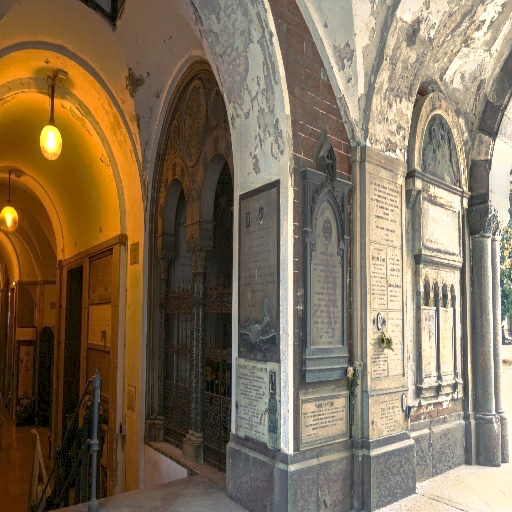
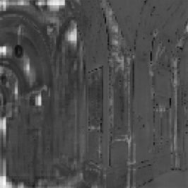
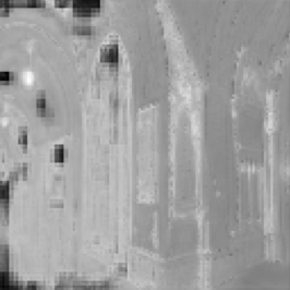
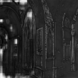
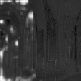
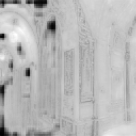
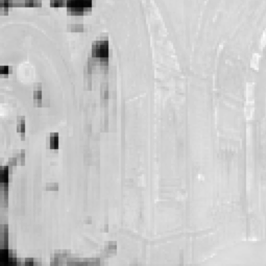
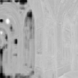
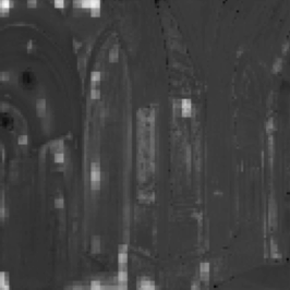
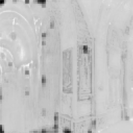
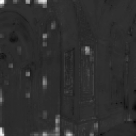
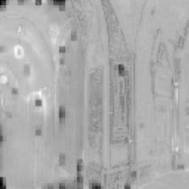
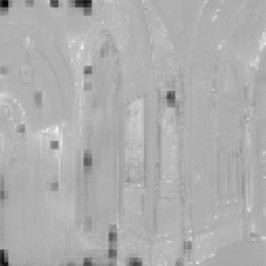
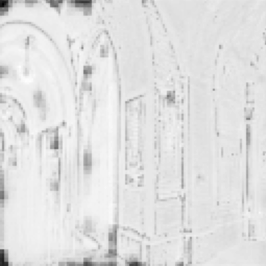
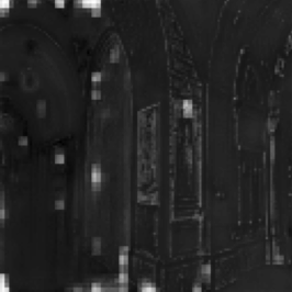
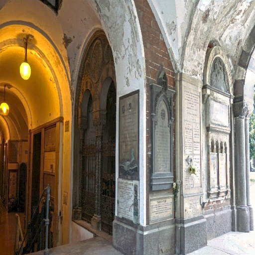
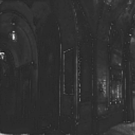
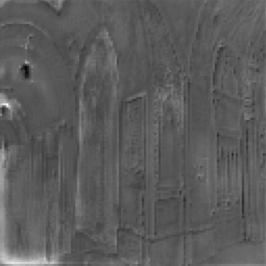
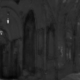
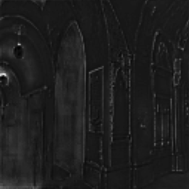
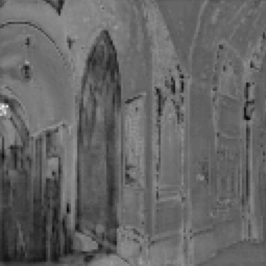
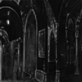
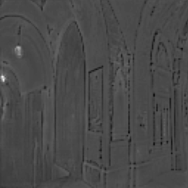
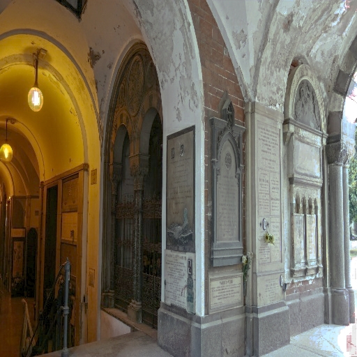
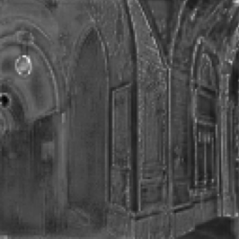
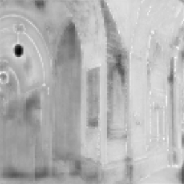
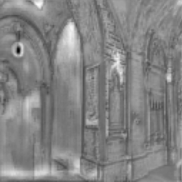
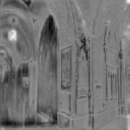
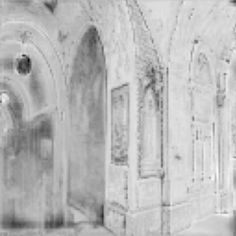
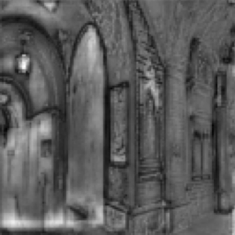
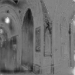
Figure 3: Illustration of feature maps learned at the Att. 4 layer of the MQN depicted in Figure 2. The rows show in order results obtained without using an attention mechanism, followed by using SA, CSA and CA. The first column shows the predicted HDR image $\hat{H}$ and the rest show the feature maps learned at different channels of the Att. 4 layer.

Table 1: (Left) Analyses of accuracy and latency measurements (on the SN20E990) for different attention mechanisms. None indicates that no attention mechanism is used and B indicates backbone. (Right) Analyses of accuracy for different loss combinations.. Blue and red indicate the best and the second best accuracy, respectively.

Attention Latency B (ms) PSNR-$TM$ SSIM-$TM$ None 11.55 $\pm$ 0.27 20.76 $\pm$ 3.21 0.8440 $\pm$ 0.0741 SA 11.68 $\pm$ 0.49 21.12 $\pm$ 3.03 0.8333 $\pm$ 0.0800 CSA 12.17 $\pm$ 0.25 20.75 $\pm$ 3.06 0.8559 $\pm$ 0.0597 CAB 12.40 $\pm$ 0.32 21.25 $\pm$ 3.11 0.8782 $\pm$ 0.0520

Loss PSNR-$TM$ SSIM-$TM$ (i) $\mathcal{L}1$ 20.00 $\pm$ 3.10 0.8295 $\pm$ 0.0646 (ii) $\mathcal{L}_{1}$, $\mathcal{L}_{2}$ 19.96 $\pm$ 3.05 0.8281 $\pm$ 0.0656 (iii) $\mathcal{L}_{1}$, $\mathcal{L}_{2}$, $\mathcal{L}_{CS}$ 20.22 $\pm$ 3.02 0.8268 $\pm$ 0.0625 (iv) $\mathcal{L}_{1}$, $\mathcal{L}_{2}$, $\mathcal{L}_{CS}$, $\mathcal{L}_{FR}$ 21.25 $\pm$ 3.11 0.8782 $\pm$ 0.0520 (v) $\mathcal{L}_{1}$, $\mathcal{L}_{FR}$ 21.19 $\pm$ 2.85 0.8261 $\pm$ 0.0832 (vi) $\mathcal{L}_{2}$, $\mathcal{L}_{FR}$ 21.53 $\pm$ 2.92 0.8343 $\pm$ 0.0675 (vii) $\mathcal{L}_{1}$, $\mathcal{L}_{2}$, $\mathcal{L}_{FR}$ 21.54 $\pm$ 2.85 0.8538 $\pm$ 0.0597

4.2 Ablation Studies

In this section, we study ablations with regard to various attention mechanisms, the quantization schemes, loss functions and deployment of MQN to hardware platforms for efficient mobile ITM.

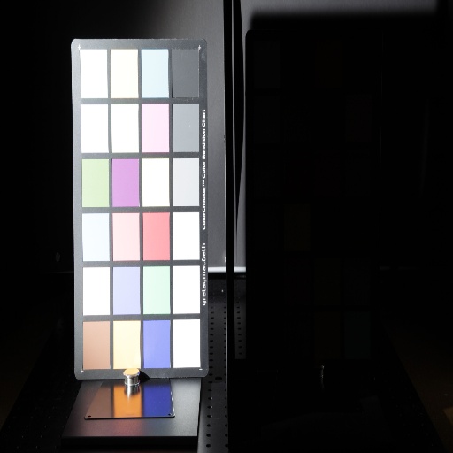
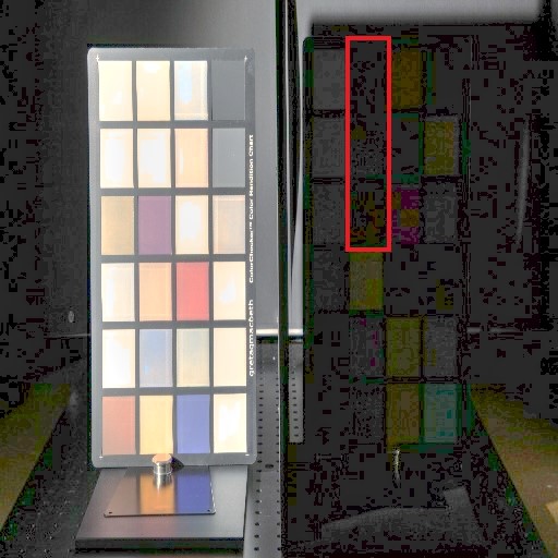
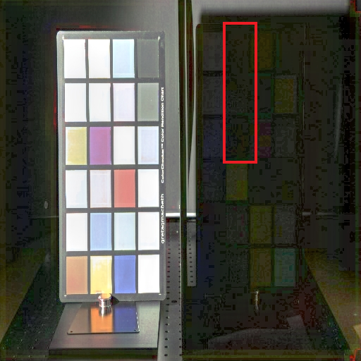
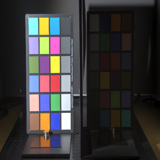
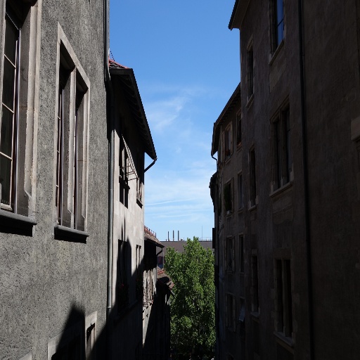
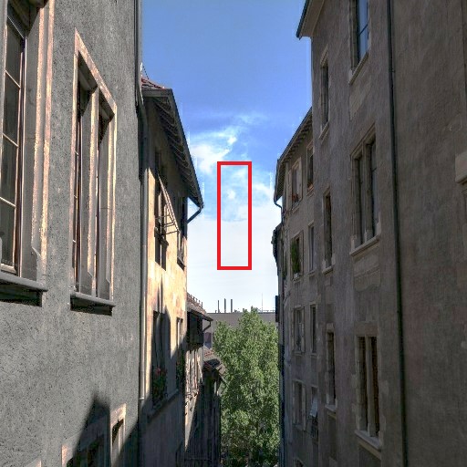
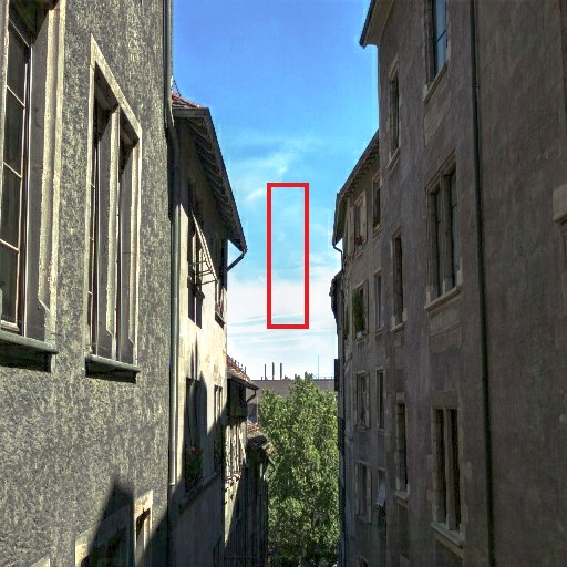
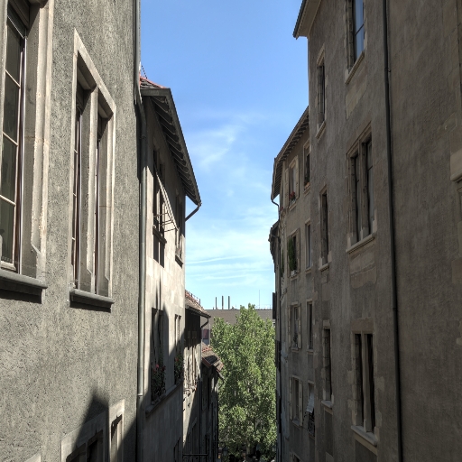
Input $I$.                   $\hat{H}$ wo/$\mathcal{L}_{FR}$.                   $\hat{H}$ w/$\mathcal{L}_{FR}$.                   Ground-truth ${H}$.

Figure 4: Visual analyses of the effect of training models with and without using $\mathcal{L}_{FR}$ on predictions $\hat{H}$. It helps models gain structural coherency and improve color details.

Table 2: Results obained using different quantization schemes. Latency (L.) is measured on the deployment platform (SN20E990).

Backbone Head L. Backbone (ms) L. Head (ms) PSNR-$T$ SSIM-$T$ Quant. Dynamic 11.52 $\pm$ 0.82 9.63 $\pm$ 0.12 21.25 $\pm$ 3.11 0.8782 $\pm$ 0.05 Quant. Float32 11.52 $\pm$ 0.82 20.95 $\pm$ 0.99 21.34 $\pm$ 3.08 0.8793 $\pm$ 0.05 Float32 Float32 21.13 $\pm$ 0.42 20.95 $\pm$ 0.99 21.58 $\pm$ 3.14 0.8727 $\pm$ 0.05

Attention Mechanisms. We explore different attention mechanisms specified in Section 3.1. Results given in Table 1 show that accuracy increases when moving from SA to CAB, which provides the best accuracy with an increase of $3\%$ on SSIM, albeit with an increase in latency of $\approx 1$ ms. We examine the features learned using different attention mechanisms in Figure 3. We observe that better feature representations of edges and surfaces are learned when models are trained using CSA and CA. For instance, in both cases, the lamp is well captured with large feature activation values, enabling the dimming effect in the prediction.

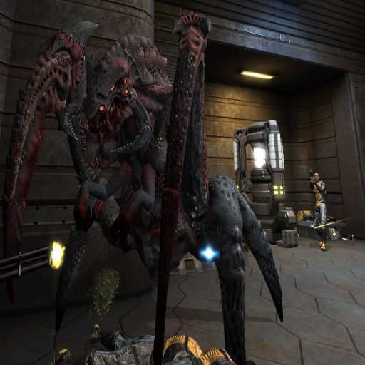
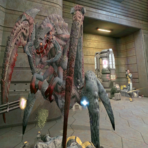
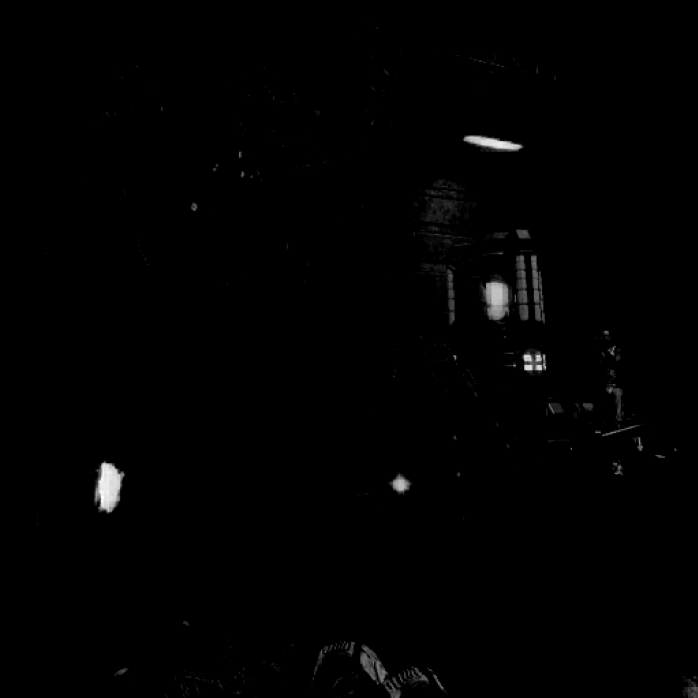
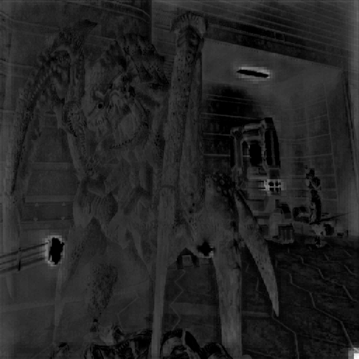
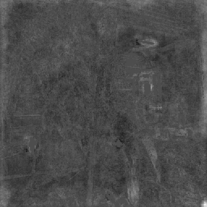
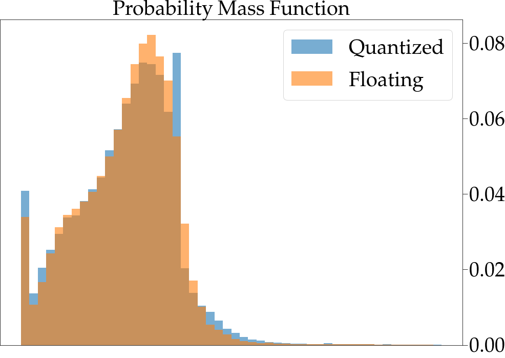
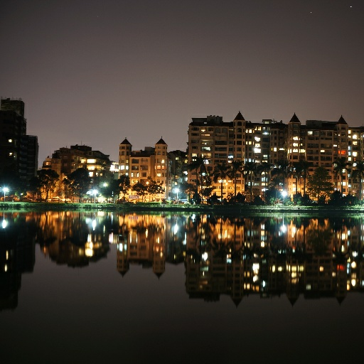
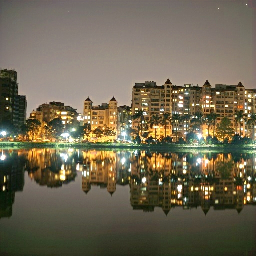
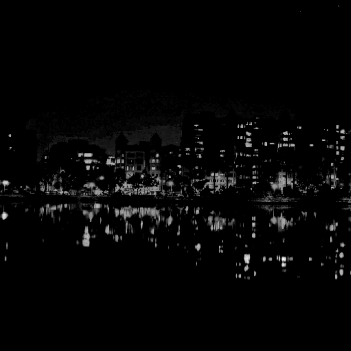
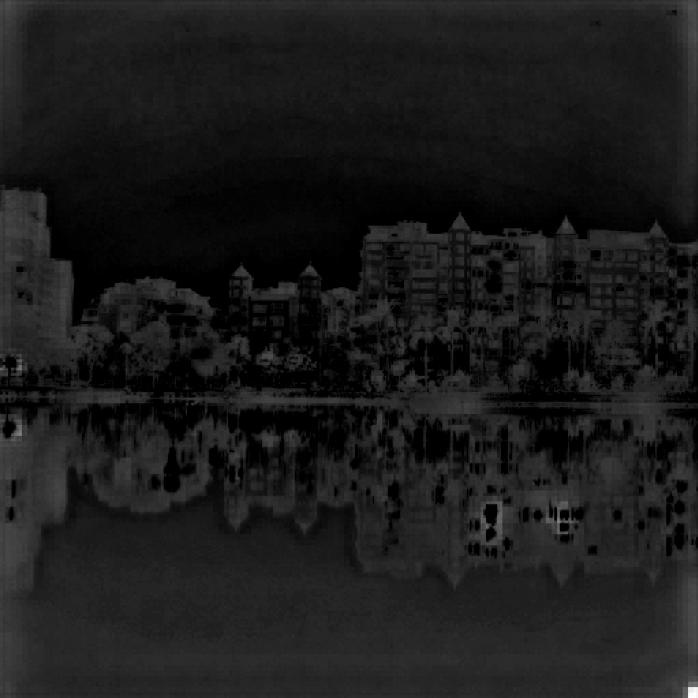
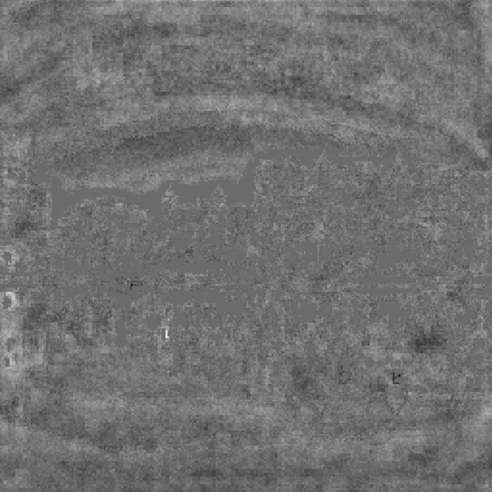
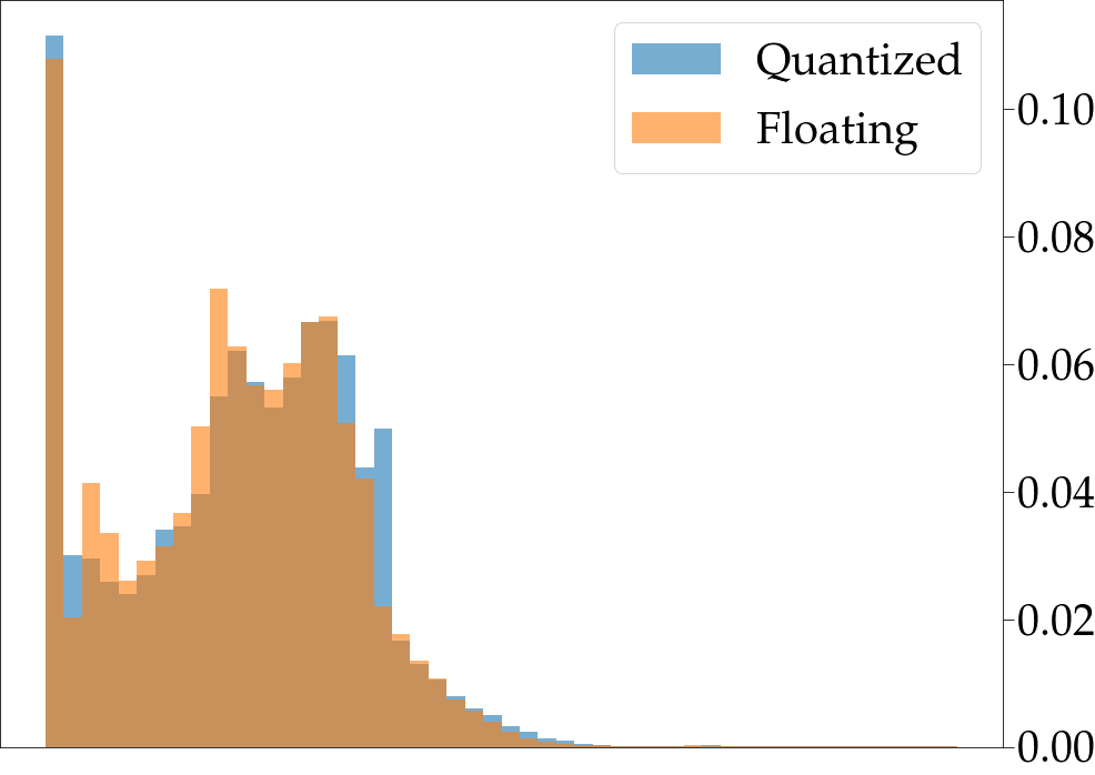
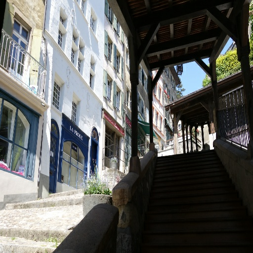
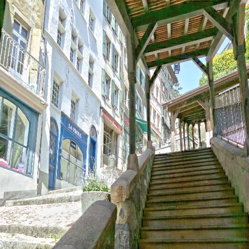
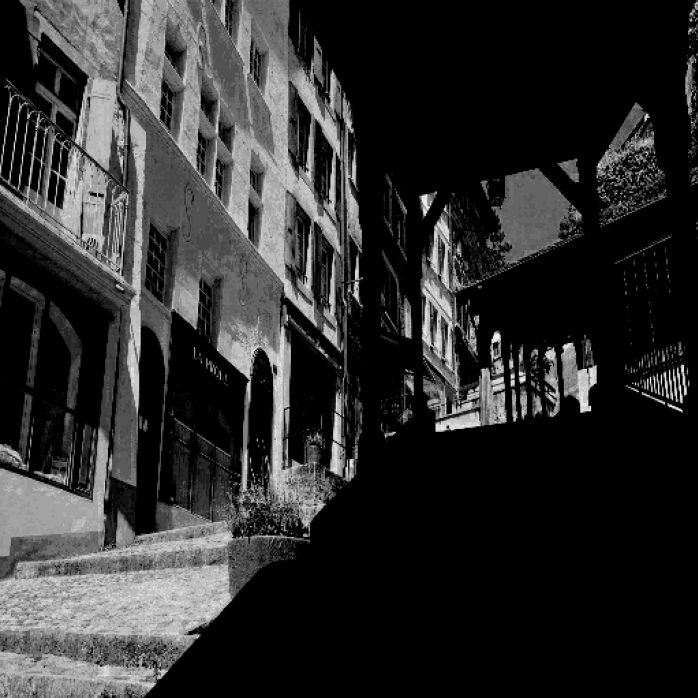
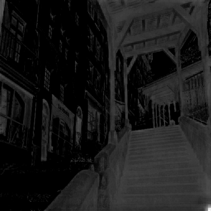
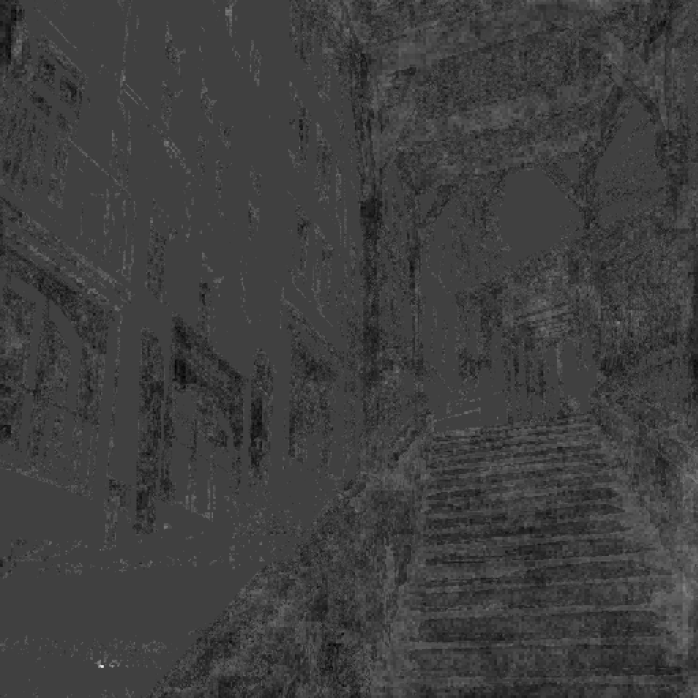
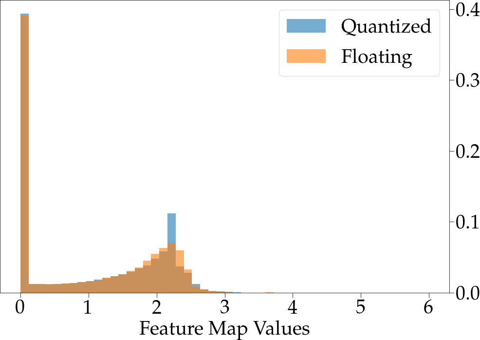
a) $I$.               b) $\hat{H}$.              c) $f_{1}$.              d) $f_{2}$.             e) $\Delta f_{2}$.          f) PMFs.

Figure 5: Analyses of the quantized $Q(\mathbf{f})$ and floating point $F(\mathbf{f})$ features $\mathbf{f}$ learned by the MQN at the ConvBnReLU3 layer at Figure 2 using a) three sample input images with b) predictions $\hat{H}$. Visualization of (c) the first channel $f_{1}$ and (d) the second channel $f_{2}$ of $\mathbf{f}$, (e) the difference map $\Delta f_{2}=\|Q(f_{2})-F(f_{2})\|_{1}$. We show the probability mass function (PMF) of $Q(f_{2})$ and $F(f_{2})$ in (f).

Quantization Schemes. Next, we study the behavior of features $\mathbf{f}$ learned at the interface between the backbone and the head (i.e., at the ConvBnReLU 3 layer depicted in Figure 2), as well as how quantization affects the interface and the head. In Table 2, we analyze how the performance and latency of models change for different quantization methods. The results show that the proposed quantization scheme enables to obtain similar PSNR/SSIM accuracy whilst showing improvements in latency.

In order to analyze the effect of quantization on statistical properties of features, we compute histograms approximating probability mass functions (PMFs) of features and their quantized versions. The results given in Figure 5.e show that distributions of quantized features $Q(\mathbf{f})$ and features with floating point values $F(\mathbf{f})$ have similar distributions. This result suggests that the quantization scheme preserves statistical information of features.

We also study what is learned in the interface as well as the effect of the network on a computer graphics image. In Figure 5 (c and d), we present two feature maps $f_{1}$ and $f_{2}$ corresponding to two channels of $\mathbf{f}$. The maps show that two very different representations are learned in these channels: in (c) light sources are identified, striking its relevancy for the ITM task, while in (d) general edge structures are learned. Moreover, we can see in the first row, as well as in Figure 1, that the network can be applied to computer graphics images without having special artifacts or distortions, opening the door for employment of MQN in computer graphics.

Loss functions. We analyze the effect of using different loss functions defined in Section 3.3 in Table 1. The results show that employing $\mathcal{L}_{FR}$ with $\mathcal{L}_{CS}$ and $\mathcal{L}_{2}$ increases accuracy substantially. Meanwhile, $\mathcal{L}_{CS}$ and $\mathcal{L}_{2}$ seem to provide a slightly negative effect on their own. Moreover, as observed in Figure 4, adding the FR loss to $\mathcal{L}_{1}$, $\mathcal{L}_{2}$, and $\mathcal{L}_{CS}$ helps improve color details and structural coherency.

Table 3: Comparison with other state-of-the-art single image HDR reconstruction methods. Performance metric and latency values reproduced with the same evaluation criteria and original codes. Blue and red indicates the best and second best accuracy. P. indicates number of parameters, L. M. indicates latency for mobile, M. RAM the maximum RAM memory consumed by the model, and O. the numer of operations in multiply-accumulate units. Performance values are given in HDRVDP-Q score. *FHDR[Khan et al.(2019)Khan, Khanna, and Raman] uses recurrence: the present value is computed taking into account two iterations.

Model	P. (M)	L. GPU (ms)	L. M. (ms)	O. (GMAC)	M. RAM (MB)	HDR-Eye	Raise-1K	HDR-Real
HDRCNN [Eilertsen et al.(2017)Eilertsen, Kronander, Denes, Mantiuk, and Unger]	29.44	247	-	30.35	-	51.16 $\pm$ 4.43	51.89 $\pm$ 2.77	45.56 $\pm$ 8.18
SingleHDR [Liu et al.(2020)Liu, Lai, Chen, Kao, Yang, Chuang, and Huang]	29.01	976	-	112.75	-	53.05 $\pm$ 5.08	51.69 $\pm$ 2.56	48.72 $\pm$ 4.03
FHDR [Khan et al.(2019)Khan, Khanna, and Raman]	0.571	54	4970 $\pm$ 434	72.34*	832.40	51.41 $\pm$ 6.72	53.13 $\pm$ 1.71	45.82 $\pm$ 8.67
HDRUnet [Chen et al.(2021b)Chen, Liu, Zhang, Qiao, and Dong]	1.651	17	808 $\pm$ 22	23.42	353.46	50.32 $\pm$ 4.07	51.42 $\pm$ 3.35	44.60 $\pm$ 7.30
ExpandNet [Marnerides et al.(2018)Marnerides, Bashford-Rogers, Hatchett, and Debattista]	0.45	21	474 $\pm$ 7	13.66	262.77	50.52 $\pm$ 3.94	51.83 $\pm$ 1.68	44.86 $\pm$ 8.21
DeepHDR [Santos et al.(2020)Santos, Ren, and Kalantari]	51.545	17	238 $\pm$ 4	18.94	251.17	51.11 $\pm$ 4.45	51.66 $\pm$ 2.79	45.81 $\pm$ 8.34
TwoStage [Sharif et al.(2021)Sharif, Naqvi, Biswas, and Sungjun]	1.088	32	3338 $\pm$ 456	54.91	397.41	49.68 $\pm$ 3.7	52.95 $\pm$ 2.36	43.46 $\pm$ 7.55
Ours (best)	0.928	11	21 $\pm$ 1	0.5	9.45	51.59 $\pm$ 4.61	51.81 $\pm$ 1.56	45.15 $\pm$ 8.15

Deployment Platforms. In the experimental analyses, we used CPU as our main deployment hardware platform. However, as our objective has been to develop a well performing but efficient model employing mixed quantization, attention, and efficient operations, our model can also be extended to other hardware platforms. For this reason, we also deploy our model to the GPU (Arm $Mali^{TM}$-G77 MP11) of SN20E990, elucidating the flexibility of our model with regards to deployment of MQN models on platforms with different hardware configurations. We obtained a latency of 10.5 ms for our backbone and 9.3 ms for our high precision head, improving our results even further and showcasing the hardware flexibility for implementation of our MQN.

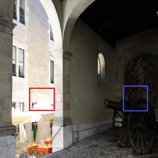
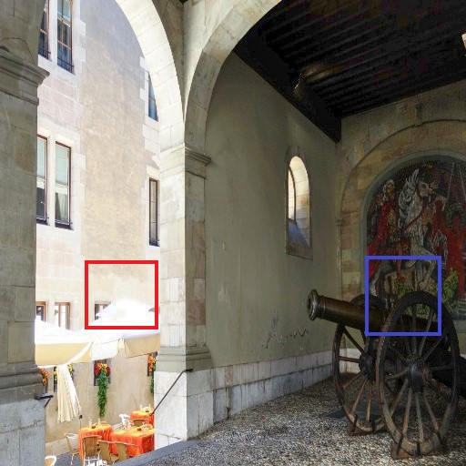
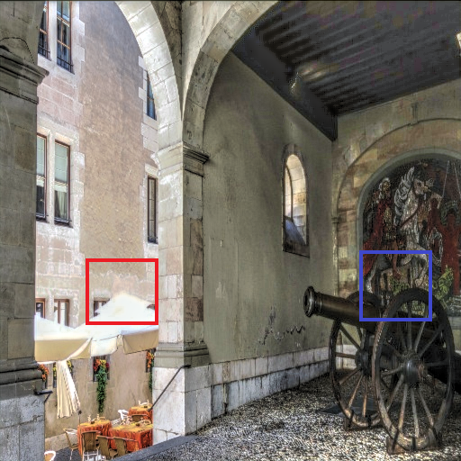
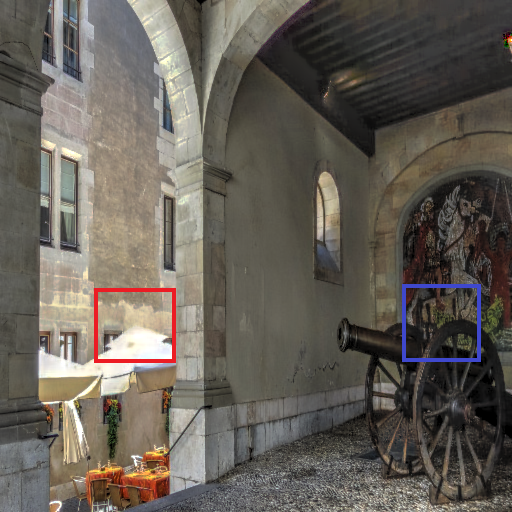
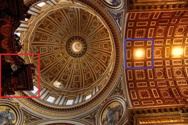
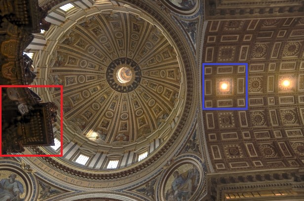
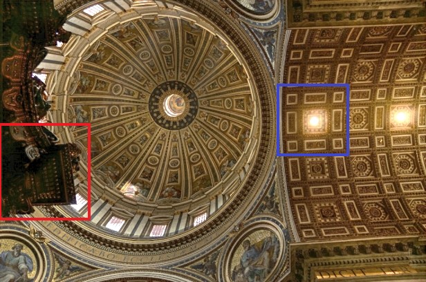
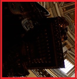
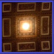
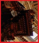
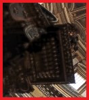
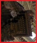
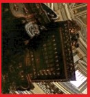
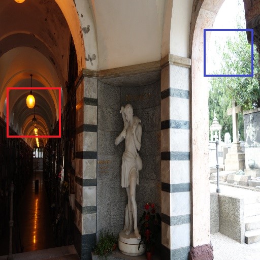
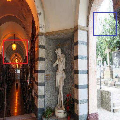
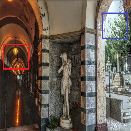
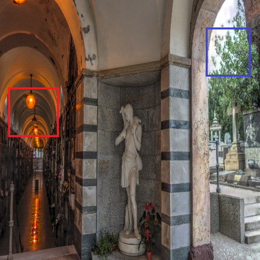
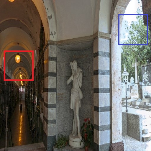
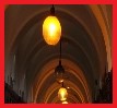
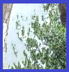
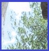
Figure 6: Visual comparison of results obtained using, from left to right; input LDR images, HDRCNN [Eilertsen et al.(2017)Eilertsen, Kronander, Denes, Mantiuk, and Unger], ExpandNet [Marnerides et al.(2018)Marnerides, Bashford-Rogers, Hatchett, and Debattista], SingleHDR [Liu et al.(2020)Liu, Lai, Chen, Kao, Yang, Chuang, and Huang] and our proposed MQN. All images are produced with Balanced TMO from the suite Photomatix [(2017)], similarly to [Liu et al.(2020)Liu, Lai, Chen, Kao, Yang, Chuang, and Huang].

4.3 Comparison with State-of-the-art Methods

In Table 3, we compare accuracy, latency, and size of models trained using MQN and state-of-the-art methods. We selected competing methods according to two criteria: (1) We considered methods that promised a reasonable accuracy-latency trade-off [Chen et al.(2021b)Chen, Liu, Zhang, Qiao, and Dong, Santos et al.(2020)Santos, Ren, and Kalantari] due to their simplicity, to evaluate the efficiency gain introduced with our method. (2) To estimate the cost of adding efficiency as a factor in network design, we compared MQN to state-of-the-art or baseline methods [Liu et al.(2020)Liu, Lai, Chen, Kao, Yang, Chuang, and Huang, Eilertsen et al.(2017)Eilertsen, Kronander, Denes, Mantiuk, and Unger] that did not take accuracy-efficiency trade-off into account. The results show that MQN models provide accuracy (HDRVDP-Q score) on par with the larger state-of-the-art models and with a notable reduction in latency and RAM consumption.

In terms of latency, our MQN provides the fastest model, both in experiments conducted on GPU and mobile deployment platforms. Comparison of the latency of the models on the GPU platform is not fair, since our MQN model uses 8-bit integer quantization and employs depthwise convolutions which are not suited for GPU platforms [Sandler et al.(2018)Sandler, Howard, Zhu, Zhmoginov, and Chen]. To obtain a fair comparison on the mobile deployment platform, we adapt the four methods HDRUNet [Chen et al.(2021b)Chen, Liu, Zhang, Qiao, and Dong], ExpandNet [Marnerides et al.(2018)Marnerides, Bashford-Rogers, Hatchett, and Debattista], DeepHDR [Santos et al.(2020)Santos, Ren, and Kalantari] and TwoStage [Sharif et al.(2021)Sharif, Naqvi, Biswas, and Sungjun] that perform the fastest inference on the GPU. The results show that the difference between the latency of our MQN models and these four models increases further on the mobile platform. More precisely, our MQN model is running in real-time ( 21ms) while others run from a quarter of a second ( DeepHDR with 238ms) to more than 3 seconds (TwoStage with 3338ms). The same trend is observed with memory consumption (maximum RAM MB) where our model stands as the most efficient with a reduction of a factor of x26 or more. The main factor for such differences is employment of our MQ scheme with computationally efficient components, such as IRLB blocks. These facts, along with learning representations of HDR content over the input, enables us to obtain a faster model with similar accuracy. However, other models use methods that hinder efficient deployment, such as by utilising images with same resolution [Marnerides et al.(2018)Marnerides, Bashford-Rogers, Hatchett, and Debattista, Sharif et al.(2021)Sharif, Naqvi, Biswas, and Sungjun], inefficient network composition [Liu et al.(2020)Liu, Lai, Chen, Kao, Yang, Chuang, and Huang], convolution operations and special blocks [Chen et al.(2021b)Chen, Liu, Zhang, Qiao, and Dong, Santos et al.(2020)Santos, Ren, and Kalantari].

In Figure 6, we compare the ITM models visually. In the analyses, our MQN model performs well with good quality in under-exposed regions. For instance, our MQN model recovers details better than others as seen in the detail of the image in row one. In the case of over-exposed regions, our model can recover details better than HDRCNN [Eilertsen et al.(2017)Eilertsen, Kronander, Denes, Mantiuk, and Unger] and similarly to ExpandNet [Marnerides et al.(2018)Marnerides, Bashford-Rogers, Hatchett, and Debattista] as seen in the lamp, tree and tent details. Although SingleHDR [Liu et al.(2020)Liu, Lai, Chen, Kao, Yang, Chuang, and Huang] performs slightly better on over-exposed regions, the SingleHDR model has 29 M parameters and takes almost a second to perform inference on a desktop GPU, while our model is 29x times smaller and almost 100x faster.

5 Conclusion

In this work, we proposed a novel DNN-based method called Mixed Quantization Network (MQN), for computationally efficient ITM. The proposed MQN has produced competitive accuracy with better computational efficiency compared to the state-of-the-art, being the first DNN-based single image ITM method targeting computationally efficient mobile ITM. Moreover, we have proven the flexibility of our framework by deploying it to both CPU and GPU platforms. Future work could consider addressing optimization of latency and accuracy trade-off for mobile ITM using additional network design and search methods, such as structured pruning and neural architecture search.

References

- [Reinhard et al.(2010)Reinhard, Heidrich, Debevec, Pattanaik, Ward, and Myszkowski] Erik Reinhard, Wolfgang Heidrich, Paul Debevec, Sumanta Pattanaik, Greg Ward, and Karol Myszkowski. High dynamic range imaging: acquisition, display, and image-based lighting. Morgan Kaufmann, 2010.
- [Akyüz et al.(2007)Akyüz, Fleming, Riecke, Reinhard, and Bülthoff] Ahmet Oǧuz Akyüz, Roland Fleming, Bernhard E. Riecke, Erik Reinhard, and Heinrich H. Bülthoff. Do HDR displays support LDR content? A psychophysical evaluation. ACM Transactions on Graphics (TOG), 26(3):38–es, 2007. Publisher: ACM New York, NY, USA.
- [Hanhart et al.(2014)Hanhart, Korshunov, and Ebrahimi] Philippe Hanhart, Pavel Korshunov, and Touradj Ebrahimi. Subjective evaluation of higher dynamic range video. In Applications of Digital Image Processing XXXVII, volume 9217, page 92170L. International Society for Optics and Photonics, 2014.
- [ (2020)] Statista . HDR TV shipments worldwide by region 2016-2019, 2020. URL https://www.statista.com/statistics/619634/hdr-tv-shipments-worldwide-by-region/.
- [Akenine-Möller et al.(2019)Akenine-Möller, Haines, and Hoffman] Tomas Akenine-Möller, Eric Haines, and Naty Hoffman. Real-Time Rendering. CRC Press, January 2019. ISBN 978-1-315-36200-7.
- [Debevec and Malik(1997)] Paul E. Debevec and Jitendra Malik. Recovering high dynamic range radiance maps from photographs. In Proceedings of the 24th annual conference on Computer graphics and interactive techniques, pages 369–378, 1997.
- [Gallo et al.(2015)Gallo, Troccoli, Hu, Pulli, and Kautz] Orazio Gallo, Alejandro Troccoli, Jun Hu, Kari Pulli, and Jan Kautz. Locally non-rigid registration for mobile HDR photography. In Proceedings of the IEEE Conference on Computer Vision and Pattern Recognition Workshops, pages 49–56, 2015.
- [Mantiuk et al.(2008)Mantiuk, Daly, and Kerofsky] Rafa\l Mantiuk, Scott Daly, and Louis Kerofsky. Display adaptive tone mapping. ACM Transactions on Graphics (TOG), 27(3):1–10, 2008. Publisher: ACM New York, NY, USA.
- [Drago et al.(2003)Drago, Myszkowski, Annen, and Chiba] Frédéric Drago, Karol Myszkowski, Thomas Annen, and Norishige Chiba. Adaptive logarithmic mapping for displaying high contrast scenes. In Computer graphics forum, volume 22, pages 419–426. Wiley Online Library, 2003. Issue: 3.
- [Reinhard et al.(2002)Reinhard, Stark, Shirley, and Ferwerda] Erik Reinhard, Michael Stark, Peter Shirley, and James Ferwerda. Photographic tone reproduction for digital images. In Proceedings of the 29th annual conference on Computer graphics and interactive techniques, pages 267–276, 2002.
- [Eilertsen et al.(2016)Eilertsen, Unger, and Mantiuk] Gabriel Eilertsen, Jonas Unger, and Rafal K. Mantiuk. Evaluation of tone mapping operators for HDR video. In High Dynamic Range Video, pages 185–207. Elsevier, 2016.
- [Banterle et al.(2006)Banterle, Ledda, Debattista, and Chalmers] Francesco Banterle, Patrick Ledda, Kurt Debattista, and Alan Chalmers. Inverse tone mapping. In Proc. of the 4th Int. Conf. on Computer Graphics and Interactive Techniques in Australasia and Southeast Asia, pages 349–356, 2006.
- [Rempel et al.(2007)Rempel, Trentacoste, Seetzen, Young, Heidrich, Whitehead, and Ward] Allan G. Rempel, Matthew Trentacoste, Helge Seetzen, H. David Young, Wolfgang Heidrich, Lorne Whitehead, and Greg Ward. Ldr2hdr: on-the-fly reverse tone mapping of legacy video and photographs. ACM transactions on graphics (TOG), 26(3):39–es, 2007. Publisher: ACM New York, NY, USA.
- [Kuo et al.(2012)Kuo, Tang, and Chien] Pin-Hung Kuo, Chi-Sun Tang, and Shao-Yi Chien. Content-adaptive inverse tone mapping. In 2012 Visual Communications and Image Processing, pages 1–6. IEEE, 2012.
- [Huo et al.(2014)Huo, Yang, Dong, and Brost] Yongqing Huo, Fan Yang, Le Dong, and Vincent Brost. Physiological inverse tone mapping based on retina response. The Visual Computer, 30(5):507–517, 2014. Publisher: Springer.
- [Masia et al.(2009)Masia, Agustin, Fleming, Sorkine, and Gutierrez] Belen Masia, Sandra Agustin, Roland W. Fleming, Olga Sorkine, and Diego Gutierrez. Evaluation of reverse tone mapping through varying exposure conditions. ACM Transactions on Graphics (TOG), 28(5):1–8, 2009. Publisher: ACM New York, NY, USA.
- [Banterle et al.(2009)Banterle, Ledda, Debattista, Bloj, Artusi, and Chalmers] Francesco Banterle, Patrick Ledda, Kurt Debattista, Marina Bloj, Alessandro Artusi, and Alan Chalmers. A psychophysical evaluation of inverse tone mapping techniques. In Computer Graphics Forum, volume 28, pages 13–25. Wiley Online Library, 2009. Issue: 1.
- [Serrano et al.(2016)Serrano, Heide, Gutierrez, Wetzstein, and Masia] Ana Serrano, Felix Heide, Diego Gutierrez, Gordon Wetzstein, and Belen Masia. Convolutional sparse coding for high dynamic range imaging. In Computer Graphics Forum, volume 35, pages 153–163. Wiley Online Library, 2016. Issue: 2.
- [Eilertsen et al.(2017)Eilertsen, Kronander, Denes, Mantiuk, and Unger] Gabriel Eilertsen, Joel Kronander, Gyorgy Denes, Rafa\l K. Mantiuk, and Jonas Unger. HDR image reconstruction from a single exposure using deep CNNs. ACM transactions on graphics (TOG), 36(6):1–15, 2017. Publisher: ACM New York, NY, USA.
- [Kim et al.(2020)Kim, Lee, Jo, and Kang] Jung Hee Kim, Siyeong Lee, Soyeon Jo, and Suk-Ju Kang. End-to-End Differentiable Learning to HDR Image Synthesis for Multi-exposure Images. arXiv preprint arXiv:2006.15833, 2020.
- [ (2021)] Microsoft Corporation . Auto HDR Preview for PC Available Today, March 2021. URL https://devblogs.microsoft.com/directx/auto-hdr-preview-for-pc-available-today/.
- [Endo et al.(2017)Endo, Kanamori, and Mitani] Yuki Endo, Yoshihiro Kanamori, and Jun Mitani. Deep reverse tone mapping. ACM Transactions on Graphics (TOG), 36(6):1–10, 2017. Publisher: ACM New York, NY, USA.
- [Marnerides et al.(2018)Marnerides, Bashford-Rogers, Hatchett, and Debattista] Demetris Marnerides, Thomas Bashford-Rogers, Jonathan Hatchett, and Kurt Debattista. Expandnet: A deep convolutional neural network for high dynamic range expansion from low dynamic range content. In Computer Graphics Forum, volume 37, pages 37–49. Wiley Online Library, 2018. Issue: 2.
- [Liu et al.(2020)Liu, Lai, Chen, Kao, Yang, Chuang, and Huang] Yu-Lun Liu, Wei-Sheng Lai, Yu-Sheng Chen, Yi-Lung Kao, Ming-Hsuan Yang, Yung-Yu Chuang, and Jia-Bin Huang. Single-Image HDR Reconstruction by Learning to Reverse the Camera Pipeline. In Proceedings of the IEEE/CVF Conference on Computer Vision and Pattern Recognition, pages 1651–1660, 2020.
- [Lee et al.(2018a)Lee, An, and Kang] Siyeong Lee, Gwon Hwan An, and Suk-Ju Kang. Deep chain hdri: Reconstructing a high dynamic range image from a single low dynamic range image. IEEE Access, 6:49913–49924, 2018a. Publisher: IEEE.
- [Khan et al.(2019)Khan, Khanna, and Raman] Zeeshan Khan, Mukul Khanna, and Shanmuganathan Raman. FHDR: HDR Image Reconstruction from a Single LDR Image using Feedback Network. arXiv preprint arXiv:1912.11463, 2019.
- [Zhang et al.(2018)Zhang, Li, Li, Wang, Zhong, and Fu] Yulun Zhang, Kunpeng Li, Kai Li, Lichen Wang, Bineng Zhong, and Yun Fu. Image Super-Resolution Using Very Deep Residual Channel Attention Networks. In Vittorio Ferrari, Martial Hebert, Cristian Sminchisescu, and Yair Weiss, editors, Computer Vision – ECCV 2018, Lecture Notes in Computer Science, pages 294–310, Cham, 2018. Springer International Publishing. ISBN 978-3-030-01234-2. 10.1007/978-3-030-01234-2_18.
- [Masia et al.(2017)Masia, Serrano, and Gutierrez] Belen Masia, Ana Serrano, and Diego Gutierrez. Dynamic range expansion based on image statistics. Multimedia Tools and Applications, 76(1):631–648, January 2017. ISSN 1573-7721. 10.1007/s11042-015-3036-0. URL https://doi.org/10.1007/s11042-015-3036-0.
- [Zhou et al.(2020)Zhou, Zhao, Han, Xu, Xu, Huang, and Shi] Chu Zhou, Hang Zhao, Jin Han, Chang Xu, Chao Xu, Tiejun Huang, and Boxin Shi. UnModNet: Learning to Unwrap a Modulo Image for High Dynamic Range Imaging. Advances in Neural Information Processing Systems, 33, 2020.
- [Ning et al.(2018)Ning, Xu, Song, Xie, and Zhang] Shiyu Ning, Hongteng Xu, Li Song, Rong Xie, and Wenjun Zhang. Learning an inverse tone mapping network with a generative adversarial regularizer. In 2018 IEEE International Conference on Acoustics, Speech and Signal Processing (ICASSP), pages 1383–1387. IEEE, 2018.
- [Yang et al.(2018)Yang, Xu, Song, Zhang, Wei, and Lau] Xin Yang, Ke Xu, Yibing Song, Qiang Zhang, Xiaopeng Wei, and Rynson WH Lau. Image correction via deep reciprocating HDR transformation. In Proceedings of the IEEE Conference on Computer Vision and Pattern Recognition, pages 1798–1807, 2018.
- [Zhang and Lalonde(2017)] Jinsong Zhang and Jean-François Lalonde. Learning high dynamic range from outdoor panoramas. In Proceedings of the IEEE International Conference on Computer Vision, pages 4519–4528, 2017.
- [Vien and Lee(2021)] An Gia Vien and Chul Lee. Single-Shot High Dynamic Range Imaging via Multiscale Convolutional Neural Network. IEEE Access, 2021. Publisher: IEEE.
- [Ye et al.(2021)Ye, Huo, Liu, and Li] Nianjin Ye, Yongqing Huo, Shuaicheng Liu, and Hanlin Li. Single Exposure High Dynamic Range Image Reconstruction Based on Deep Dual-Branch Network. IEEE Access, 9:9610–9624, 2021. Publisher: IEEE.
- [Sharif et al.(2021)Sharif, Naqvi, Biswas, and Sungjun] S. M. A. Sharif, Rizwan Ali Naqvi, Mithun Biswas, and Kim Sungjun. A Two-stage Deep Network for High Dynamic Range Image Reconstruction. arXiv preprint arXiv:2104.09386, 2021.
- [Pérez-Pellitero et al.(2021)Pérez-Pellitero, Catley-Chandar, Leonardis, and Timofte] Eduardo Pérez-Pellitero, Sibi Catley-Chandar, Ales Leonardis, and Radu Timofte. NTIRE 2021 challenge on high dynamic range imaging: Dataset, methods and results. In Proceedings of the IEEE/CVF Conference on Computer Vision and Pattern Recognition, pages 691–700, 2021.
- [Akhil and Jiji(2021)] K. A. Akhil and C. V. Jiji. Single image hdr synthesis using a densely connected dilated convnet. In IEEE/CVF Conference on Computer Vision and Pattern Recognition Workshops, 2021.
- [Chen et al.(2021a)Chen, Zhang, Sun, Gao, Michelini, and Wu] Guannan Chen, Lijie Zhang, Mengdi Sun, Yan Gao, Pablo Navarrete Michelini, and YanHong Wu. Single-image hdr reconstruction with task-specific network based on channel adaptive RDN. In Proceedings of the IEEE/CVF Conference on Computer Vision and Pattern Recognition, pages 398–403, 2021a.
- [Pan and Vento(2021)] Edwin Pan and Anthony Vento. MetaHDR: Model-Agnostic Meta-Learning for HDR Image Reconstruction. arXiv preprint arXiv:2103.12545, 2021.
- [Yan et al.(2019)Yan, Gong, Shi, van den Hengel, Shen, Reid, and Zhang] Qingsen Yan, Dong Gong, Qinfeng Shi, Anton van den Hengel, Chunhua Shen, Ian Reid, and Yanning Zhang. Attention-Guided Network for Ghost-Free High Dynamic Range Imaging. In 2019 IEEE/CVF Conference on Computer Vision and Pattern Recognition (CVPR), pages 1751–1760. IEEE, 2019.
- [Niu et al.(2020)Niu, Wu, Liu, Guo, and Lau] Yuzhen Niu, Jianbin Wu, Wenxi Liu, Wenzhong Guo, and Rynson WH Lau. HDR-GAN: HDR image reconstruction from multi-exposed ldr images with large motions. arXiv preprint arXiv:2007.01628, 2020.
- [Yan et al.(2020)Yan, Zhang, Liu, Zhu, Sun, Shi, and Zhang] Q. Yan, L. Zhang, Y. Liu, Y. Zhu, J. Sun, Q. Shi, and Y. Zhang. Deep HDR Imaging via A Non-Local Network. IEEE Transactions on Image Processing, 29:4308–4322, 2020. ISSN 1941-0042. 10.1109/TIP.2020.2971346. Conference Name: IEEE Transactions on Image Processing.
- [Wu et al.(2018)Wu, Xu, Tai, and Tang] Shangzhe Wu, Jiarui Xu, Yu-Wing Tai, and Chi-Keung Tang. Deep high dynamic range imaging with large foreground motions. In Proceedings of the European Conference on Computer Vision (ECCV), pages 117–132, 2018.
- [Kalantari and Ramamoorthi(2017)] Nima Khademi Kalantari and Ravi Ramamoorthi. Deep high dynamic range imaging of dynamic scenes. ACM Trans. Graph., 36(4):144–1, 2017. URL https://cseweb.ucsd.edu/~viscomp/projects/SIG17HDR/.
- [Liu et al.(2021)Liu, Lin, Li, Rao, Jiang, Han, Fan, Sun, and Liu] Zhen Liu, Wenjie Lin, Xinpeng Li, Qing Rao, Ting Jiang, Mingyan Han, Haoqiang Fan, Jian Sun, and Shuaicheng Liu. ADNet: Attention-guided Deformable Convolutional Network for High Dynamic Range Imaging. arXiv preprint arXiv:2105.10697, 2021.
- [Prabhakar et al.(2021)Prabhakar, Senthil, Agrawal, Babu, and Gorthi] K. Ram Prabhakar, Gowtham Senthil, Susmit Agrawal, R. Venkatesh Babu, and Rama Krishna Sai S Gorthi. Labeled From Unlabeled: Exploiting Unlabeled Data for Few-Shot Deep HDR Deghosting. In Proceedings of the IEEE/CVF Conference on Computer Vision and Pattern Recognition (CVPR), pages 4875–4885, June 2021.
- [Lee et al.(2018b)Lee, Hwan An, and Kang] Siyeong Lee, Gwon Hwan An, and Suk-Ju Kang. Deep recursive hdri: Inverse tone mapping using generative adversarial networks. In Proceedings of the European Conference on Computer Vision (ECCV), pages 596–611, 2018b.
- [Sudhakaran et al.(2020)Sudhakaran, Escalera, and Lanz] Swathikiran Sudhakaran, Sergio Escalera, and Oswald Lanz. Gate-shift networks for video action recognition. In Proceedings of the IEEE/CVF Conference on Computer Vision and Pattern Recognition (CVPR), June 2020.
- [Sandler et al.(2018)Sandler, Howard, Zhu, Zhmoginov, and Chen] Mark Sandler, Andrew Howard, Menglong Zhu, Andrey Zhmoginov, and Liang-Chieh Chen. Mobilenetv2: Inverted residuals and linear bottlenecks. In Proceedings of the IEEE conference on computer vision and pattern recognition, pages 4510–4520, 2018.
- [Howard et al.(2017)Howard, Zhu, Chen, Kalenichenko, Wang, Weyand, Andreetto, and Adam] Andrew G. Howard, Menglong Zhu, Bo Chen, Dmitry Kalenichenko, Weijun Wang, Tobias Weyand, Marco Andreetto, and Hartwig Adam. Mobilenets: Efficient convolutional neural networks for mobile vision applications. CoRR, abs/1704.04861, 2017. URL http://arxiv.org/abs/1704.04861.
- [Tan and Le(2020)] Mingxing Tan and Quoc V. Le. EfficientNet: Rethinking Model Scaling for Convolutional Neural Networks. arXiv:1905.11946 [cs, stat], September 2020. URL http://arxiv.org/abs/1905.11946. arXiv: 1905.11946.
- [Liu(2020)] Timothy Liu. Depth-wise Separable Convolutions: Performance Investigations, 2020. URL https://tlkh.dev/depsep-convs-perf-investigations/.
- [Lee et al.(2020)Lee, Kang, and Ha] Jaeseong Lee, Duseok Kang, and Soonhoi Ha. S3nas: Fast npu-aware neural architecture search methodology. arXiv preprint arXiv:2009.02009, 2020.
- [Choi and Rhu(2020)] Yujeong Choi and Minsoo Rhu. Prema: A predictive multi-task scheduling algorithm for preemptible neural processing units. In 2020 IEEE International Symposium on High Performance Computer Architecture (HPCA), pages 220–233. IEEE, 2020.
- [Ronneberger et al.(2015)Ronneberger, Fischer, and Brox] Olaf Ronneberger, Philipp Fischer, and Thomas Brox. U-net: Convolutional networks for biomedical image segmentation. In International Conference on Medical image computing and computer-assisted intervention, pages 234–241. Springer, 2015.
- [Zhou et al.(2018)Zhou, Siddiquee, Tajbakhsh, and Liang] Zongwei Zhou, Md Mahfuzur Rahman Siddiquee, Nima Tajbakhsh, and Jianming Liang. Unet++: A nested u-net architecture for medical image segmentation. In Deep learning in medical image analysis and multimodal learning for clinical decision support, pages 3–11. Springer, 2018.
- [Woo et al.(2018)Woo, Park, Lee, and Kweon] Sanghyun Woo, Jongchan Park, Joon-Young Lee, and In So Kweon. Cbam: Convolutional block attention module. In Proceedings of the European conference on computer vision (ECCV), pages 3–19, 2018.
- [Vaswani et al.(2017)Vaswani, Shazeer, Parmar, Uszkoreit, Jones, Gomez, Kaiser, and Polosukhin] Ashish Vaswani, Noam Shazeer, Niki Parmar, Jakob Uszkoreit, Llion Jones, Aidan N. Gomez, \Lukasz Kaiser, and Illia Polosukhin. Attention is all you need. In Advances in neural information processing systems, pages 5998–6008, 2017.
- [Huang and Belongie(2017)] Xun Huang and Serge Belongie. Arbitrary style transfer in real-time with adaptive instance normalization. In Proceedings of the IEEE International Conference on Computer Vision, pages 1501–1510, 2017.
- [Jacob et al.(2018)Jacob, Kligys, Chen, Zhu, Tang, Howard, Adam, and Kalenichenko] Benoit Jacob, Skirmantas Kligys, Bo Chen, Menglong Zhu, Matthew Tang, Andrew Howard, Hartwig Adam, and Dmitry Kalenichenko. Quantization and training of neural networks for efficient integer-arithmetic-only inference. In Proceedings of the IEEE Conference on Computer Vision and Pattern Recognition, pages 2704–2713, 2018.
- [Baskin et al.(2018)Baskin, Liss, Zheltonozhskii, Bronstein, and Mendelson] Chaim Baskin, Natan Liss, Evgenii Zheltonozhskii, Alex M. Bronstein, and Avi Mendelson. Streaming architecture for large-scale quantized neural networks on an FPGA-based dataflow platform. In 2018 IEEE International Parallel and Distributed Processing Symposium Workshops (IPDPSW), pages 162–169. IEEE, 2018.
- [Gysel et al.(2018)Gysel, Pimentel, Motamedi, and Ghiasi] Philipp Gysel, Jon Pimentel, Mohammad Motamedi, and Soheil Ghiasi. Ristretto: A Framework for Empirical Study of Resource-Efficient Inference in Convolutional Neural Networks. IEEE Transactions on Neural Networks and Learning Systems, 29(11):5784–5789, November 2018. ISSN 2162-2388. 10.1109/TNNLS.2018.2808319.
- [Johnson et al.(2016)Johnson, Alahi, and Fei-Fei] Justin Johnson, Alexandre Alahi, and Li Fei-Fei. Perceptual losses for real-time style transfer and super-resolution. In European conference on computer vision, pages 694–711. Springer, 2016.
- [Funt and Shi(2010)] Brian Funt and Lilong Shi. The effect of exposure on MaxRGB color constancy. In Human Vision and Electronic Imaging XV, volume 7527, page 75270Y. International Society for Optics and Photonics, 2010. URL https://www2.cs.sfu.ca/~colour/data/funt_hdr/.
- [Ward(2006)] Greg Ward. High dynamic range image encodings, 2006. URL http://www.anyhere.com/gward/hdrenc/pages/originals.html. Publisher: Citeseer.
- [ (2015)] Rafael Mantiuk . PFSTools. High Dynamic Range Images and Videos, 2015. URL http://pfstools.sourceforge.net/hdr_gallery.html.
- [Hasinoff et al.(2016)Hasinoff, Sharlet, Geiss, Adams, Barron, Kainz, Chen, and Levoy] Samuel W. Hasinoff, Dillon Sharlet, Ryan Geiss, Andrew Adams, Jonathan T. Barron, Florian Kainz, Jiawen Chen, and Marc Levoy. Burst photography for high dynamic range and low-light imaging on mobile cameras. ACM Transactions on Graphics, 35(6):192:1–192:12, November 2016. ISSN 0730-0301. 10.1145/2980179.2980254. URL https://doi.org/10.1145/2980179.2980254.
- [Nemoto et al.(2015)Nemoto, Korshunov, Hanhart, and Ebrahimi] Hiromi Nemoto, Pavel Korshunov, Philippe Hanhart, and Touradj Ebrahimi. Visual attention in LDR and HDR images. In 9th International Workshop on Video Processing and Quality Metrics for Consumer Electronics (VPQM), 2015. Issue: CONF.
- [Dang-Nguyen et al.(2015)Dang-Nguyen, Pasquini, Conotter, and Boato] Duc-Tien Dang-Nguyen, Cecilia Pasquini, Valentina Conotter, and Giulia Boato. Raise: A raw images dataset for digital image forensics. In Proceedings of the 6th ACM Multimedia Systems Conference, pages 219–224, 2015.
- [Mantiuk et al.(2011)Mantiuk, Kim, Rempel, and Heidrich] Rafa\l Mantiuk, Kil Joong Kim, Allan G. Rempel, and Wolfgang Heidrich. HDR-VDP-2: A calibrated visual metric for visibility and quality predictions in all luminance conditions. ACM Transactions on graphics (TOG), 30(4):1–14, 2011. Publisher: ACM New York, NY, USA.
- [Chen et al.(2021b)Chen, Liu, Zhang, Qiao, and Dong] Xiangyu Chen, Yihao Liu, Zhengwen Zhang, Yu Qiao, and Chao Dong. HDRUNet: Single Image HDR Reconstruction with Denoising and Dequantization. arXiv:2105.13084, 2021b.
- [Santos et al.(2020)Santos, Ren, and Kalantari] Marcel Santana Santos, Tsang Ing Ren, and Nima Khademi Kalantari. Single image HDR reconstruction using a CNN with masked features and perceptual loss. arXiv preprint arXiv:2005.07335, 2020.
- [ (2017)] HDRSoft Ltd. . Photo Editing Software for HDR & Real Estate Photography | Photomatix, 2017. URL https://www.hdrsoft.com/.