Can Scale-free Network Growth with Triad Formation Capture Simplicial Complex Distributions in Real Communication Networks?

Abstract

In recent years, there has been a growing recognition that higher-order structures are important features in real-world networks. A particular class of structures that has gained prominence is known as a simplicial complex. Despite their application to complex processes such as social contagion and novel measures of centrality, not much is currently understood about the distributional properties of these complexes in communication networks. Furthermore, it is also an open question as to whether an established growth model, such as scale-free network growth with triad formation, is sophisticated enough to capture the distributional properties of simplicial complexes. In this paper, we use empirical data on five real-world communication networks to propose a functional form for the distributions of two important simplicial complex structures. We also show that, while the scale-free network growth model with triad formation captures the form of these distributions in networks evolved using the model, the best-fit parameters are significantly different between the real network and its simulated equivalent. An auxiliary contribution is an empirical profile of the two simplicial complexes in these five real-world networks.

Introduction

Complex systems have undergone intense, interdisciplinary study in recent decades, with network science (Lewis 2011), (Barabási et al. 2016) having emerged as a viable framework for understanding complexity. While early studies in network science tended to be limited to lower-order structures like dyadic links or edges (Seidman 1983), (Milward and Provan 1998), (Motter, Zhou, and Kurths 2005), (Hagberg, Swart, and S Chult 2008) (and later, triangles), a recent and growing body of research has revealed that deep insights can be gained from the systematic study of non-simple networks, multi-layer networks (Mitchison and Durbin 1989) and ‘higher-order’ structures (Xu, Wickramarathne, and Chawla 2016) in simple networks.

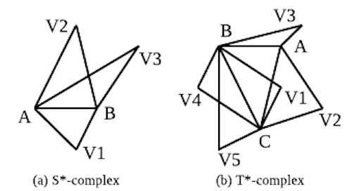
Figure 1: Illustration of an S* simplicial complex and T* simplicial complex, defined in the text.

One such higher-order structure that continues to undergo study is a simplicial complex (often just referred to as a ‘complex’) (Hofmann, Curtiss, and McNally 2016), (Barbarossa, Sardellitti, and Ceci 2018), (Torres and Bianconi 2020). The study of simplicial complexes first took root in mathematics (especially, algebraic topology) (Milnor 1957), (Faridi 2002), (Maria et al. 2014), (Costa and Farber 2016), (Knill 2020), but in the last several years, have found practical applications in network science (as discussed in Related Work). Figure 1 provides a practical example of two such simplicial complexes that have been studied in the literature, especially in theoretical biology and protein interaction networks. Due to space limitations, we do not provide a full formal definition; a good reference is (Estrada and Ross 2018), who detailed some of their properties and even proposed centrality measures due to their importance. An S-complex is defined by a ‘central’ edge A-B, with one or more triangles sharing that edge. A T-complex is similar but the central unit is a triangle (A-B-C). Furthermore, non-central (or peripheral) triangles in a T-complex should not also participate in quads with the central triangle i.e., given central triangle A-B-C and peripheral triangle A-B-V3, there should be no link between V3 and C in a valid T-complex. As we detail subsequently, the adjacency factor of either an S*- or T*-complex is the number of triangles flanking the central structure (an edge or triangle respectively).

Given the growing recognition that these two structures play an important role in real networks, and with this brief background in place, we propose to investigate the following research questions (RQs):

RQ1: In real-world communication networks, what are the respective distributions of S*- and T*-complexes? Can good functional fits be found for these distributions?

RQ2: Can (and to what extent) the scale-free network growth model (with triad formation) accurately capture these distributions? Or are additional parameters and steps (beyond triad formation) needed to model these higher-order structural properties in real-world networks?

Related Work

Communication networks, as well as many other natural and social networks, have the scale-free topology in common. The preferential attachment model (Eisenberg and Levanon 2003), (Vázquez 2003) has been suggested as a candidate network evolution or ‘growth’ model to yield such topologies in complex networks by formalizing the intuition that highly connected nodes increase their connectivity faster than their less connected peers. The degree distribution of such networks has been shown to exhibit power–law scaling (Jeong, Néda, and Barabási 2003).

While the degree distribution provides a glimpse into the structure of a complex network, models that extend pairwise relationships to multi-node relationships occurring in the system, and that allow for higher-order interactions, have been known for some time now to be important for capturing the richness and higher-order topological structures in real networks (Iacopini et al. 2019), (Albert and Barabási 2002), (Torres et al. 2020), (Boccaletti et al. 2006), (Guilbeault, Becker, and Centola 2018). In particular, in the last several years, simplicial complexes have been widely used to analyze aspects of diverse multilayer systems, including social relation (Wang et al. 2020), social contagion (Pastor-Satorras et al. 2015), protein interaction (Serrano, Hernández-Serrano, and Gómez 2020), linguistic categorization (Gong et al. 2011), and transportation (Lin and Ban 2013). New measurements, such as simplicial degree (Serrano, Hernández-Serrano, and Gómez 2020), simplicial degree based centralities (Serrano and Gómez 2020), (Estrada and Ross 2018), and random walks (Schaub et al. 2020) have all been proposed to not only measure the relevance of a simplicial community and the quality of higher-order connections, but also the dynamical properties of simplicial networks.

However, to the best of our knowledge, the distributional properties of such complexes, especially in the context of communication networks, have not been studied so far. A methodology for conducting such studies has also been lacking. While the former is our primary goal in this short paper, we also shed some light on the latter through our proposed methodology.

Methodology

Since our primary goal in this paper is to understand whether (and to what extent) the scale-free network growth (with triad formation) model can accurately and empirically capture the two simplicial complexes described in the introduction, we first briefly recap the details of the growth model below. Full details are provided in (Holme and Kim 2002).

Scale-free Network Growth with Triad Formation

Networks with the power-law degree distribution have been classically modeled by the scale-free network model of Barabási and Albert (BA) (Barabási and Albert 1999). In the original BA model, the initial condition is a network with $n_{0}$ nodes. In each growth timestep, an incoming node $v$ is connected using $m$ edges to existing nodes in the network. The connections are determined using preferential attachment (PA), wherein an edge between $v$ and another node $w$ in the network is established with probability proportional to the degree of $w$.

The growth model informally described above is known to generate a network with the power-law degree distribution; however, other work has found that such networks lack triadic properties (including observed clustering coefficient) in real networks. In order to incorporate such higher-order properties, the growth step in BA model was extended by (Holme and Kim 2002) to include a triad formation (TF) step. Specifically, given that an an edge between nodes $v$ and $w$ was attached using preferential attachment, an edge is also established from $v$ to a random neighbor of $w$ with some probability. If all neighbors of $w$ are connected to $v$, this step does not apply.

In summary, when a ‘new’ node $v$ comes in, a PA step will first be performed, and then a TF step will be performed with probability $P_{t}$ (in other words, the probability of PA without TF is $1-P_{t}$). These two steps are performed repeatedly per incoming node until $m$ edges are added to the network. $P_{t}$ is the control parameter in the model. It has been shown to have a linear relationship with the network’s average (over all nodes) clustering coefficient. The clustering coefficient is a measure of the degree of clustering, the clustering coefficient $\gamma_{v}$ of node $v$ is given by $\frac{|\mathcal{E}(\Gamma_{v})|}{\frac{k_{v}(k_{v}-1)}{2}}$, where $|\mathcal{E}(\Gamma_{v})|$ is the number of edges that exist between node $v$’s neighbors.

Table 1: Details on five real communication networks (including average clustering coefficient) used in this paper.

	Num. Nodes	Num. Edges	Avg. CC.
Email-Enron	36,265	111,179	0.16
Email-DNC	1,866	4,384	0.21
Email-EU	32,430	54,397	0.11
Uni. of Kiel	57,189	92,442	0.04
Phone Calls	36,595	56,853	0.14

Adjacency Factor

To understand the distributional properties of the S*- and T*- complexes in the generated network versus real communication networks, we use the notion of the adjacency factor. From the earlier definition, we know that an S*-complex is defined by a ‘central’ edge (A-B in Figure 1 (a)) that is adjacent to a certain number of triangles. Given an edge in the network, therefore, we denote the adjacency factor (with respect to S*-complexes) as the (maximal) number of triangles adjacent to that edge. For example, the adjacency factor of edge A-B in Figure 1 (a) would be 3, not 1 or 2. While we record adjacency factors of 0 also to obtain a continuous distribution, only cases where adjacency factor is greater than 0 constitute valid S*-complexes.

Similarly, the adjacency factor (with respect to T*-complexes) applies to triangles in the network. For every triangle A-B-C (see Figure 1 (b)), the adjacency factor is the (maximal) number of triangles adjacent to it in the T*-complex configuration. If no (non-quad) triangles are adjacent to any of the edges of the central A-B-C triangle, then the adjacency factor is 0, meaning that the triangle does not technically participate in a T*-complex.

Hence, depending on whether we are studying and comparing S*- or T*-complex distributions, an adjacency factor can be computed for each edge and each triangle (respectively) in the network. We compute a frequency distribution over these adjacency factors to better contrast these higher-order structures in the grown versus the actual networks from a distributional standpoint.

Experiments

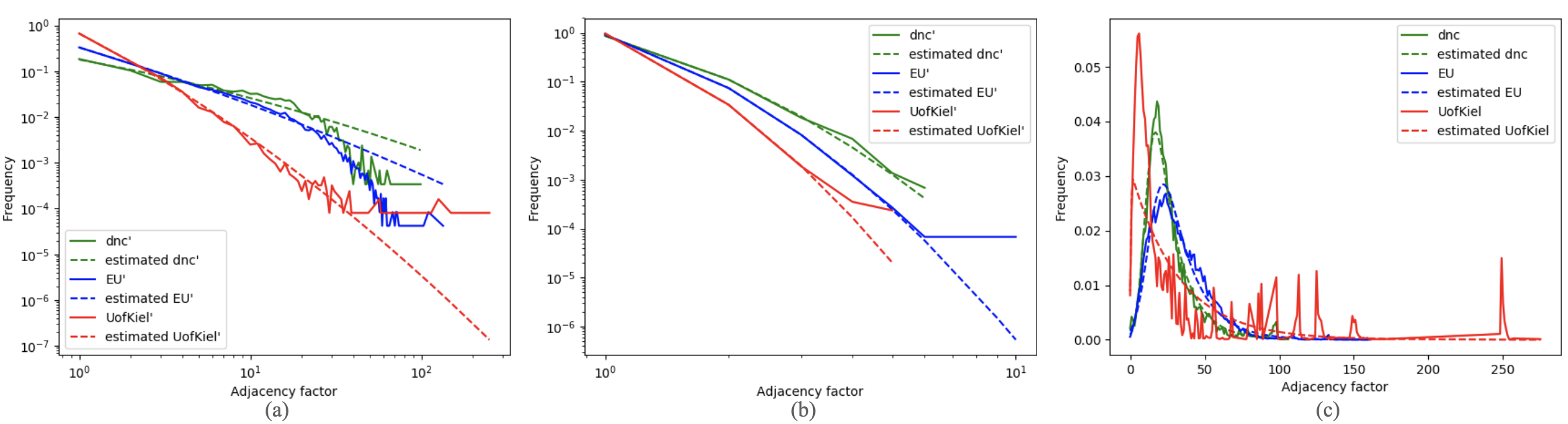
Figure 2: Frequency distribution of adjacency factors (described in the text) of (a) S*- and (c) T*-complexes in the real Email-EU, Email-DNC, and University of Kiel email networks (distributions for the other two datasets are qualitatively similar). S*-complex distributions for the generated networks are shown in (b), with the PA-TF generated networks sharing the same number of nodes, edges, and average clustering coefficient (Table 1) as their real counterparts. Due to space limitation, T*-complex frequency distribution of adjacency-factors for the generated networks is not included here. In all plots, the actual adjacency-factors distribution is always shown as a solid line and the corresponding estimated function with best-fit parameters (Equations 1 and 2) as a dashed line. Both (a) and (b) are on a log-log (with base 10) scale.

We use five publicly available communication networks in our experiments, including Enron email communication network (Email-Enron), 2016 Democratic National Committee email leak network (Email-DNC), a European research institution email data network (Email-EU), the email network based on traffic data collected for 112 days at University of Kiel, Germany (Ebel, Mielsch, and Bornholdt 2002), and a mobile communication network (Song et al. 2010). Details are shown in Table 1. These networks are available publicly and some (such as Enron) have been extensively studied, but to our knowledge studies involving simplicial complexes and their properties have been non-existent with respect to these communication networks. While our primary goal here is not to study these properties for these specific networks, a secondary contribution of the results that follow is that they do shed some light on the extent and distribution of such complexes in these networks.

In the Introduction, we had introduced two separate (but related) research questions. Below, we discuss both individually, although both rely on a shared set of results.

RQ1: For each network, using the numbers of nodes and edges, and the observed average clustering coefficient, we generate 10 networks using the PA-based growth model (with TF). We obtain the frequency distributions (normalized to resemble a probability distribution) of adjacency factors of T*- and S*-complexes in both the real and generated networks, and visualize these distributions in Figure 2. Besides the direct comparison between the distribution curves, the figures suggest two functions that could fit the distributions (for the S*- and T*-complexes respectively):

$$f_{S*}(x;a,b,c)=c(bx^{-a})^{\log x}$$ (1)

$$f_{T*}(x;\mu,\lambda,\sigma)=\frac{\lambda}{2}e^{\frac{\lambda}{2}(2\mu+\lambda\sigma^{2}-2x)}erfc(\frac{\mu+\lambda\sigma^{2}-x}{\sqrt{2}\sigma})$$ (2)

where $erfc(x)=\frac{2}{\sqrt{\pi}}\int_{x}^{\infty}e^{-t^{2}}dt$.

Both functional fits were discovered empirically using the Enron dataset as a ‘development’ set; however, as we show in response to RQ2, the functions fit quite consistently for all five datasets (but with different parameters, of course), although the first function diverges after a point (when the long tail begins). A theoretical basis for the functions is an interesting open question. We note that the second function is an Exponentially modified Gaussian (EMG) distribution, which is an important and general class of models for capturing skewed distributions. It has been broadly studied in mathematics, and has found empirical applications as well (Foley and Dorsey 1984).

	Equation 1				Equation 2
	real / grown				real / grown
	$a$ / $\overline{a^{\prime}}$	$b$ / $\overline{b^{\prime}}$	$c$ / $\overline{c^{\prime}}$	$MND$ / $\overline{MND^{\prime}}$ / ref. $MND$	$\lambda$ / $\overline{\lambda^{\prime}}$	$\mu$ / $\overline{\mu^{\prime}}$	$\sigma$ / $\overline{\sigma^{\prime}}$	$MND$ / $\overline{MND^{\prime}}$ / ref. $MND$
Email-Enron	0.25 / 0.82	0.75 / 0.59	0.19 / 0.53	0.68 / 0.79 / 0.71	0.02 / 0.21	6.82 / 0.87	5.08 / 0.79	0.37 / 0.83 / 0.91
Email-DNC	0.07 / 1.25	0.50 / 0.15	0.18 / 0.85	0.64 / 0.33 / 0.71	0.07 / 0.76	10.86 / 0.00	5.06 / 0.00	0.33 / 0.53 / 0.90
Email-EU	0.06 / 1.79	0.33 / 0.09	0.33 / 0.92	0.67 / 0.34 / 0.74	0.05 / 1.59	13.81 / 0.00	7.58 / 0.00	0.70 / 0.84 / 0.90
Uni. of Kiel	0.16 / 1.35	0.15 / 0.02	0.67 / 0.97	0.49 / 0.47 / 0.55	0.03 / 3.13	0.37 / 0.00	0.57 / 0.00	0.68 / 1.07 / 0.74
Phone Calls	0.65 / 1.78	0.44 / 0.11	0.55 / 0.90	0.56 / 0.28 / 0.84	0.43 / 1.42	0.00 / 0.00	0.00 / 0.00	0.44 / 0.79 / 0.76

Table 2: Best-fit parameter estimates for both Equations 1 and 2. The MND and reference baseline is described in the text.

RQ2: We tabulate the best-fit parameters for each real world network, and the generated networks, in Table 2. For the real world networks, there is only one set of best-fit estimates. For the generated networks there are ten best-fit estimates per parameter (since we generate 10 networks per real-world network), for which we report the average in the table. We also compute a 2-tailed Student’s t-test and found that, for all parameters and all networks, the generated networks’ (averaged) parameter is significantly different from the corresponding real network’s best-fit parameter at the 99% level. This suggests, intriguingly, that despite the similarities between distributions in Figure 2 (a) and (b) (i.e., between the real and generated networks) the best-fit parameters (for real networks) are significantly different in both cases.

Of course, this does not answer the question as to whether the functions that we empirically discovered and suggested in Equations 1 and 2 are good approximations or models for the actual distributions. To quantify such a ‘goodness of fit’ between an actual frequency distribution curve (whether for the real network or the generated networks) and the curve obtained by using the models suggested in Equation 1 or 2 (with best-fit parameter estimates), we compute a metric called Mean Normalized Deviation (MND). This metric is modeled closely after the root mean square error (RMSE) metric. Given an actual curve $f$ and a modeled curve $f^{\prime}$, defined on a common support (x-axis) $X=\{x_{1},x_{2},\ldots x_{n}\}$, the MND is given by:

$$MND(f,f^{\prime},X)=\frac{1}{|X|}\sum_{x\in X}\frac{|f^{\prime}(x)-f(x)|}{f(x)}$$ (3)

Note that the lower the MND, the better $f^{\prime}$ fits $f$ on support $X$. The MND can never be negative for a positive function $f$, but it has no upper bound. Hence, a reference is needed. Since we are not aware of any other candidate functional fits for the simplicial complex distributions in the literature, we use a simple (but functionally effective) baseline, namely the horizontal curve $y=c$, where $c$ is a constant that is selected to roughly coincide with the long-tail of the corresponding real network’s distribution.

In Table 2, we report not just the MNDs of the real and grown networks, but also the corresponding reference MND. Because of the significant long tails in Figure 2, this MND is already expected to be low. We find, however, that with only three exceptions (over both equations) for the generated networks (and none for the real networks) does the reference fit the actual distributions better than our proposed models (through a lower MND), despite being optimized to almost coincide with the long tail. Interestingly, Equation 2 has (much) lower MND scores for the real network compared to the grown networks, as well as the reference function. As we noted earlier, Equation 1 did not seem to be capturing the long tail accurately. We hypothesize that a piecewise function, where Equation 1 is only used for modeling the short tail of the S*-complex frequency distribution, may be a better fit. In all cases, investigating the theory of this phenomenon is a promising area of investigation for complex systems research.

Conclusion

Simplicial complexes have become important in the last several years for modeling and reasoning about higher-order structures in real networks. Many questions remain about these structures, including whether they are captured properly by existing (and now classic) growth models. In this paper, we showed that, for two well-known complexes, the PA-model with triad formation captures the distributional properties of the complexes, but the best-fit parameters are significantly different between the grown networks and the real communication networks. It remains an active area of research to better understand the theoretical underpinnings of our proposed functional fits for the simplicial complex distributions, and also to deduce what could be ‘added’ to the growth model to bring its parameters into alignment with the real-world network. We are also investigating the properties of other growth models with respect to accurately capturing these distributions. Finally, understanding the real-world phenomena modeled by these complexes, which are fairly common motifs in all five networks we studied, continues to be an interesting research avenue in communication (and other complex) systems.

References

- Albert and Barabási (2002) Albert, R.; and Barabási, A.-L. 2002. Statistical mechanics of complex networks. Rev. Mod. Phys., 74: 47–97.
- Barabási and Albert (1999) Barabási, A.-L.; and Albert, R. 1999. Emergence of Scaling in Random Networks. Science, 286(5439): 509–512.
- Barabási et al. (2016) Barabási, A.-L.; et al. 2016. Network science. Cambridge university press.
- Barbarossa, Sardellitti, and Ceci (2018) Barbarossa, S.; Sardellitti, S.; and Ceci, E. 2018. Learning from signals defined over simplicial complexes. In 2018 IEEE Data Science Workshop (DSW), 51–55. IEEE.
- Boccaletti et al. (2006) Boccaletti, S.; Latora, V.; Moreno, Y.; Chavez, M.; and Hwang, D.-U. 2006. Complex networks: Structure and dynamics. Physics Reports, 424(4): 175–308.
- Costa and Farber (2016) Costa, A.; and Farber, M. 2016. Random simplicial complexes. In Configuration spaces, 129–153. Springer.
- Ebel, Mielsch, and Bornholdt (2002) Ebel, H.; Mielsch, L.-I.; and Bornholdt, S. 2002. Scale-free topology of e-mail networks. Phys. Rev. E, 66: 035103.
- Eisenberg and Levanon (2003) Eisenberg, E.; and Levanon, E. Y. 2003. Preferential attachment in the protein network evolution. Physical review letters, 91(13): 138701.
- Estrada and Ross (2018) Estrada, E.; and Ross, G. J. 2018. Centralities in simplicial complexes. Applications to protein interaction networks. Journal of theoretical biology, 438: 46–60.
- Faridi (2002) Faridi, S. 2002. The facet ideal of a simplicial complex. Manuscripta Mathematica, 109(2): 159–174.
- Foley and Dorsey (1984) Foley, J. P.; and Dorsey, J. G. 1984. A review of the exponentially modified Gaussian (EMG) function: evaluation and subsequent calculation of universal data. Journal of chromatographic science, 22(1): 40–46.
- Gong et al. (2011) Gong, T.; Baronchelli, A.; Puglisi, A.; and Loreto, V. 2011. Exploring the Roles of Complex Networks in Linguistic Categorization. Artificial Life, 18(1): 107–121.
- Guilbeault, Becker, and Centola (2018) Guilbeault, D.; Becker, J.; and Centola, D. 2018. Complex contagions: A decade in review. In Complex spreading phenomena in social systems, 3–25. Springer.
- Hagberg, Swart, and S Chult (2008) Hagberg, A.; Swart, P.; and S Chult, D. 2008. Exploring network structure, dynamics, and function using NetworkX. Technical report, Los Alamos National Lab.(LANL), Los Alamos, NM (United States).
- Hofmann, Curtiss, and McNally (2016) Hofmann, S. G.; Curtiss, J.; and McNally, R. J. 2016. A complex network perspective on clinical science. Perspectives on Psychological Science, 11(5): 597–605.
- Holme and Kim (2002) Holme, P.; and Kim, B. 2002. Growing scale-free networks with tunable clustering. Physical review. E, Statistical, nonlinear, and soft matter physics, 65 2 Pt 2: 026107.
- Iacopini et al. (2019) Iacopini, I.; Petri, G.; Barrat, A.; and Latora, V. 2019. Simplicial models of social contagion. Nature communications, 10(1): 1–9.
- Jeong, Néda, and Barabási (2003) Jeong, H.; Néda, Z.; and Barabási, A.-L. 2003. Measuring preferential attachment in evolving networks. EPL (Europhysics Letters), 61(4): 567.
- Knill (2020) Knill, O. 2020. The energy of a simplicial complex. Linear Algebra and its Applications.
- Lewis (2011) Lewis, T. G. 2011. Network science: Theory and applications. John Wiley & Sons.
- Lin and Ban (2013) Lin, J.; and Ban, Y. 2013. Complex network topology of transportation systems. Transport reviews, 33(6): 658–685.
- Maria et al. (2014) Maria, C.; Boissonnat, J.-D.; Glisse, M.; and Yvinec, M. 2014. The Gudhi library: Simplicial complexes and persistent homology. In International Congress on Mathematical Software, 167–174. Springer.
- Milnor (1957) Milnor, J. 1957. The geometric realization of a semi-simplicial complex. Annals of Mathematics, 357–362.
- Milward and Provan (1998) Milward, H. B.; and Provan, K. G. 1998. Measuring network structure. Public administration, 76(2): 387–407.
- Mitchison and Durbin (1989) Mitchison, G.; and Durbin, R. 1989. Bounds on the learning capacity of some multi-layer networks. Biological Cybernetics, 60(5): 345–365.
- Motter, Zhou, and Kurths (2005) Motter, A. E.; Zhou, C.; and Kurths, J. 2005. Enhancing complex-network synchronization. EPL (Europhysics Letters), 69(3): 334.
- Pastor-Satorras et al. (2015) Pastor-Satorras, R.; Castellano, C.; Van Mieghem, P.; and Vespignani, A. 2015. Epidemic processes in complex networks. Reviews of modern physics, 87(3): 925.
- Schaub et al. (2020) Schaub, M. T.; Benson, A. R.; Horn, P.; Lippner, G.; and Jadbabaie, A. 2020. Random walks on simplicial complexes and the normalized Hodge 1-Laplacian. SIAM Review, 62(2): 353–391.
- Seidman (1983) Seidman, S. B. 1983. Network structure and minimum degree. Social networks, 5(3): 269–287.
- Serrano and Gómez (2020) Serrano, D. H.; and Gómez, D. S. 2020. Centrality measures in simplicial complexes: Applications of topological data analysis to network science. Applied Mathematics and Computation, 382: 125331.
- Serrano, Hernández-Serrano, and Gómez (2020) Serrano, D. H.; Hernández-Serrano, J.; and Gómez, D. S. 2020. Simplicial degree in complex networks. applications of topological data analysis to network science. Chaos, Solitons & Fractals, 137: 109839.
- Song et al. (2010) Song, C.; Qu, Z.; Blumm, N.; and Barabási, A.-L. 2010. Limits of Predictability in Human Mobility. Science, 327(5968): 1018–1021.
- Torres and Bianconi (2020) Torres, J. J.; and Bianconi, G. 2020. Simplicial complexes: higher-order spectral dimension and dynamics. Journal of Physics: Complexity, 1(1): 015002.
- Torres et al. (2020) Torres, L.; Blevins, A. S.; Bassett, D. S.; and Eliassi-Rad, T. 2020. The why, how, and when of representations for complex systems. arXiv preprint arXiv:2006.02870.
- Vázquez (2003) Vázquez, A. 2003. Growing network with local rules: Preferential attachment, clustering hierarchy, and degree correlations. Phys. Rev. E, 67: 056104.
- Wang et al. (2020) Wang, D.; Zhao, Y.; Leng, H.; and Small, M. 2020. A social communication model based on simplicial complexes. Physics Letters A, 384(35): 126895.
- Xu, Wickramarathne, and Chawla (2016) Xu, J.; Wickramarathne, T. L.; and Chawla, N. V. 2016. Representing higher-order dependencies in networks. Science advances, 2(5): e1600028.