Computing eigenvalues of semi-infinite quasi-Toeplitz matrices

Abstract

A quasi-Toeplitz (QT) matrix is a semi-infinite matrix of the form $A=T(a)+E$ where $T(a)$ is the Toeplitz matrix with entries $(T(a))_{i,j}=a_{j-i}$, for $a_{j-i}\in\mathbb{C}$, $i,j\geq 1$, while $E$ is a matrix representing a compact operator in $\ell^{2}$. The matrix $A$ is finitely representable if $a_{k}=0$ for $k<-m$ and for $k>n$, given $m,n>0$, and if $E$ has a finite number of nonzero entries. The problem of numerically computing eigenpairs of a finitely representable QT matrix is investigated, i.e., pairs $(\lambda,\bm{v})$ such that $A\bm{v}=\lambda\bm{v}$, with $\lambda\in\mathbb{C}$, $\bm{v}=(v_{j})_{j\in\mathbb{Z}^{+}}$, $\bm{v}\neq 0$, and $\sum_{j=1}^{\infty}|v_{j}|^{2}<\infty$. It is shown that the problem is reduced to a finite nonlinear eigenvalue problem of the kind $WU(\lambda)\bm{\beta}=0$, where $W$ is a constant matrix and $U$ depends on $\lambda$ and can be given in terms of either a Vandermonde matrix or a companion matrix. Algorithms relying on Newton’s method applied to the equation $\det WU(\lambda)=0$ are analyzed. Numerical experiments show the effectiveness of this approach. The algorithms have been included in the CQT-Toolbox [Numer. Algorithms 81 (2019), no. 2, 741–769].

1 Introduction

A quasi-Toeplitz (QT) matrix $A$ is a semi-infinite matrix that can be written as $A=T(a)+E$ where $T(a)=(t_{i,j})_{i,j\in\mathbb{Z}^{+}}$ is Toeplitz, i.e., $t_{i,j}=a_{j-i}$ for a given sequence $\{a_{k}\}_{k\in\mathbb{Z}}$, and $E$ is compact, that is, $E$ is the limit of a sequence of semi-infinite matrices $E_{i}$ of finite rank. Here, convergence means that $\lim_{i\to\infty}\|E-E_{i}\|_{s}=0$, where $\|\cdot\|_{s}$ is the operator norm induced by the vector norm $\|\bm{v}\|_{s}=(\sum_{i=1}^{\infty}|v_{i}|^{s})^{\frac{1}{s}}$, for $\bm{v}=(v_{i})_{i\in\mathbb{Z}^{+}}$, and the value of $s\geq 1$ depends on the specific context where the mathematical model originates.

Matrices of this kind are encountered in diverse applications related to semi-infinite domains. For instance, the analysis of queuing models, where buffers have infinite capacity, leads to QT matrices where the compact correction reproduces the boundary conditions of the model while the Toeplitz part describes the inner action of the stochastic process. A typical paradigm in this framework is given by random walks in the quarter plane. Some references in this regard can be found in the books [5], [26], [28], and in the more recent papers [24], [30], [31]. Another classical and meaningful example concerns the class of matrices that discretize boundary value problems by means of finite differences. In this case, the Toeplitz part of the QT matrix describes the inner action of the differential operator, while the compact correction expresses the boundary conditions imposed on the differential system. In this framework, it is worth citing the two books [19], [20], that are a relevant reference on a very close subject concerning generalized locally Toeplitz matrices (GLT) and their applications, where a rich literature is cited.

Computational aspects in the solution of matrix equations with QT matrices in bidimensional random walk have been recently investigated in [6], [7], [11], while generalizations including probabilistic models with restarts are analyzed in [8]. Other applications of QT matrices have been considered in [3], [4], [10], concerning matrix functions and means, and in [25], [32] concerning Sylvester equations. Important sources of theoretical properties of QT matrices are given in the books [12], [13], and [16]. In [9] a suitable Matlab toolbox, the CQT-toolbox, has been introduced for performing arithmetic operations with QT matrices including the four arithmetic operations and the more relevant matrix factorizations.

1.1 Main results

In this paper, we deal with the computation of the eigenvalues of QT matrices, a topic that was not covered in the CQT-Toolbox of [9]. Namely, we are interested in the design and analysis of algorithms for computing the eigenvalues $\lambda$ and the corresponding eigenvectors $\bm{v}$ of a given QT matrix $A$, that is, $\bm{v}$ is such that $A\bm{v}=\lambda\bm{v}$ and $\bm{v}\in\ell^{s}$ where $1\leq s<\infty$. Here $\ell^{s}$ is the set of vectors $\bm{x}=(x_{i})_{i\geq 1}$ such that $\|\bm{x}\|_{s}<\infty$. For the sake of simplicity, in the following we will set $s=2$ and use $\|\cdot\|$ to denote the $2$-norm. The attention is restricted to the case where $A$ is finitely representable, i.e., $A=T(a)+E$, where $T(a)$ is a band Toeplitz matrix determined by a finite number of parameters $a_{-m},\ldots,a_{n}$ for $m,n>0$, $E$ is a matrix having infinitely many rows and columns but a finite number of nonzero entries. A matrix of this kind represents a bounded linear operator from $\ell^{2}$ in $\ell^{2}$. We associate with the matrix $A$ the Laurent polynomial $a(z)=\sum_{i=-m}^{n}a_{i}z^{i}$.

Recall that the spectrum of a bounded operator $A$ is the set of $\lambda\in\mathbb{C}$ such that $A-\lambda I$ is not invertible, and the essential spectrum is the set of $\lambda\in\mathbb{C}$ such that $A-\lambda I$ is not Fredholm. We wish to point out that, not all the points of the spectrum or of the essential spectrum are necessarily eigenvalues of $A$. Moreover, while for a Toeplitz matrix $A$ the set of eigenvalues does not contain isolated points and can be explicitly determined by the image $a(\mathbb{T})$ of the unit circle $\mathbb{T}$ through the Laurent polynomial $a(z)$ and by the winding number of $a(z)-\lambda$ (see [12]), for a general QT matrix having a nontrivial compact correction the set of eigenvalues may contain a continuous part and a discrete part, the latter is formed by a set of isolated eigenvalues. As an example, see Figure 1.

Figure 1: Isolated eigenvalues (blue dots) and dense set of eigenvalues (green area) of the QT matrix associated with $a(z)=z^{-3}-3z^{-2}+2z^{-1}-2z+z^{2}+2z^{3}$ and with the correction $E=(e_{i,j})$, $e_{1,j}=-2j$, $e_{2,j}=-2(10-j)$, $e_{3,j}=-2$, for $j=1,\ldots,9$, $e_{i,j}=0$ elsewhere.

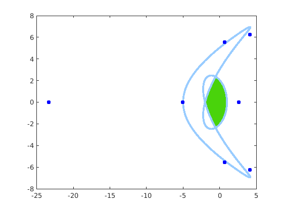
We prove that any isolated eigenvalue $\lambda$ of a QT matrix $A$ is the solution of a finite nonlinear eigenvalue problem of the form

$$WU(\lambda)\bm{\gamma}=0,\quad\bm{\gamma}\in\mathbb{C}^{p}\setminus\{0\},$$

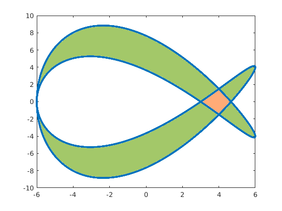
where $W$ is a $q\times k$ constant matrix and $U(\lambda)$ is a $k\times p$ matrix-valued function whose size $p$ and entries depend on $\lambda$ in an implicit way. Here $k,q>0$ are integers depending on the given matrix $A$, while $p$ is the number of zeros $\xi_{j}$, $j=1,\ldots,p$ of modulus less than 1 of the Laurent polynomial $a(z)-\lambda$. It is well-known that the value of $p$ is given by $p=m+w$ where $w$ is the winding number of $a(z)-\lambda$. Thus, it takes constant values on each connected component $\Omega$ of the set $\mathbb{C}\setminus a(\mathbb{T})$ (see Figure 2 for an example). Note that while $p$ depends on $\lambda$, it is locally constant on $\mathbb{C}\setminus a(\mathbb{T})$, and thus we will not write explicitly the dependence on $\lambda$.

We consider two different forms of $U=(u_{i,j})$: the Vandermonde version and the Frobenius version. In the former version, $U$ can be chosen as the Vandermonde matrix with entries $u_{i,j}=\xi_{j}^{i-1}$, $i=1,\ldots,k$, $j=1,\ldots,p$, provided that $\xi_{i}\neq\xi_{j}$ for $i\neq j$. In the latter, $U$ is the truncation to size $k\times p$ of the matrix $[I;G;G^{2};\ldots]$ (we adopted the Matlab notation where “;” separates block rows of the matrix), where $G=F^{p}$ is the $p$-th power of the $p\times p$ companion (Frobenius) matrix $F$ associated with the monic polynomial $s(z)=\prod_{j=1}^{p}(z-\xi_{j})=z^{p}+\sum_{j=0}^{p-1}s_{j}z^{j}$.

This formulation of the problem allows us to detect those components $\Omega$ that constitute continuous sets of eigenvalues (for $q<p$), and to design numerical algorithms for computing the isolated eigenvalues of $A$ (for $q\geq p$) by solving the corresponding nonlinear eigenvalue problem. Nonlinear eigenvalue problems have recently received much attention in the literature. Here we refer to the survey paper [22], to the subsequent paper [21], to the more recent works [18] and [23], and to the references there in.

Our algorithms follow the classical approach of applying Newton’s iteration, as done in [18] and [22], to the scalar equation $f(\lambda)\!=\!0$, where $f(\lambda)\!=\!\det(WU(\lambda))$ by relying on the Jacobi identity $f(\lambda)/f^{\prime}(\lambda)\!=\!1/\hbox{trace}((WU(\lambda))^{-1}WU^{\prime}(\lambda))$. Here, the main problem is to exploit the specific features of the function $f(\lambda)$ through the design of efficient algorithms to compute $U(\lambda)$ and $U^{\prime}(\lambda)$ in both the Vandermonde and in the Frobenius formulation. This analysis leads to the algorithmic study of some interesting computational problems such as computing the winding number of $a(z)-\lambda$, or computing the coefficients of the polynomial factor $s(z)$ having zeros of modulus less than 1 together with their derivatives with respect to $\lambda$, or computing $G=F^{p}$ and the derivative of $G^{j}$ for $j=1,2,\ldots$, with respect to $\lambda$. We will accomplish the above tasks by relying on the combination of different computational tools such as Graeffe’s iteration [29], the Wiener-Hopf factorization of $a(z)-\lambda$ computed by means of the cyclic reduction algorithm [5], and the Barnett factorization of $F^{p}$ [1].

The algorithms based on the Vandermonde and on the Frobenius versions require either the computation of the zeros of the Laurent polynomial $a(z)-\lambda$ and the selection of those zeros $\xi_{1},\ldots,\xi_{p}$ having modulus less than 1, or the computation of the coefficients of the factor $\prod_{j=1}^{p}(z-\xi_{j})$. In principle, the latter approach is less prone to numerical instabilities and avoids the theoretical difficulties encountered when there are multiple or clustered zeros. This fact is confirmed by numerical tests and analysis.

Our procedure uses Newton’s iteration as an effective tool for refining a given approximation to an eigenvalue. In order to numerically compute all the eigenvalues we have combined Newton’s iteration with a heuristic strategy based on choosing as starting approximations the eigenvalues of the $N\times N$ matrix $A_{N}$ given by the leading principal submatrix of $A$ of sufficiently large size. In fact, we may show that for any $\epsilon>0$, the $\epsilon$-pseudospectrum of $A_{N}$ gets closer to any isolated eigenvalue of $A$ as $N$ gets large.

One could argue that a large value of $N$ would provide an approximation of the isolated eigenvalues of $A$, directly. Nevertheless, our approach requires only a rough approximation of the isolated eigenvalues and thus a smaller value of $N$, followed by Newton’s iteration, to compute the eigenvalues with the same accuracy. Numerical experiments show the effectiveness of this approach: examples are shown where in order to obtain full-precision approximations of the eigenvalues of $A$ from the eigenvalues of $A_{N}$ would require large values of $N$ (of the order of millions), while starting Newton’s iteration with the eigenvalues of $A_{N}$ for moderate values of $N$ (of the order of few hundreds) provides very accurate approximations in few steps.

1.2 Paper organization

The paper is organized as follows. In Section 2 we recall some preliminary properties that are useful in the subsequent analysis. In particular, Section 2.1 deals with the eigenvalues of $T(a)$ while Section 2.2 deals with the eigenvalues of $T(a)+E$. Section 3 concerns the reduction of the original eigenvalue problem for QT operators to the form of a nonlinear eigenvalue problem for finite matrices in the Frobenius and in the Vandermonde versions. Section 4 concerns further algorithmic issues. In particular, an efficient method for computing the winding number of a Laurent polynomial is designed based on the Graeffe iteration; the problem of computing a factor of the polynomial $a(z)-\lambda$ together with its derivative with respect to $\lambda$ is analyzed relying on the Barnett factorization and on the solution of a linear system associated with a resultant matrix; morever, in the same section we prove the regularity of the function $\det(WU(\lambda))$ to which Newton’s iteration is applied. In Section 5 we investigate on the relationships between the isolated eigenvalues of $A$ and the eigenvalues of $A_{N}$ when $N$ gets large. The results of some numerical experiments are reported in Section 6. Finally, Section 7 draws the conclusions and describes some open problems.

The algorithms, implemented in Matlab, have been added to the CQT-Toolbox of [9]. The main functions are eig_single and eig_all. The former computes a single eigenvalue of a QT matrix starting from a given approximation, and, optionally, an arbitrary number of components of the corresponding eigenvector, the latter provides the computation of all the eigenvalues. Other related functions integrate the package. More information, together with the description of other auxiliary functions and optional parameters can be found at https://numpi.github.io/cqt-toolbox while the software can be downloaded at https://github.com/numpi/cqt-toolbox.

2 Preliminaries

Let $a(z)=\sum_{i=-m}^{n}a_{i}z^{i}$ be a Laurent polynomial where $a_{i}\in\mathbb{C}$ for $i=-m,\ldots,n$, and $a_{-m},a_{n}\neq 0$. Define $T(a)=(t_{i,j})_{i,j=1,2,\ldots}$, $t_{i,j}=a_{j-i}$, the Toeplitz matrix associated with $a(z)$. Given a semi-infinite matrix $E=(e_{i,j})_{i,j=1,2,\ldots}$, such that $e_{i,j}=0$ for $i>k_{1}$, or $j>k_{2}$, the matrix $A=T(a)+E$ represents a bounded linear operator from the set $\ell^{2}=\{(v_{i})_{i\in\mathbb{Z}^{+}}\,:\,v_{i}\in\mathbb{C},~{}\sum_{i=1}^{\infty}|v_{i}|^{2}<\infty\}$ to itself. Denote by $\mathcal{B}(\ell^{2})$ the set of bounded linear operators from $\ell^{2}$ to itself and by $\mathbb{T}$ the unit circle in the complex plane.

Recall that $A$ is invertible if there exists $B\in\mathcal{B}(\ell^{2})$ such that $AB=BA=I$, where $I$ is the identity on $\mathcal{B}(\ell^{2})$. Moreover, $A$ is Fredholm if there exists $B\in\mathcal{B}(\ell^{2})$ such that $AB-I$ and $BA-I$ are compact, i.e., $A$ is invertible modulo compact operators. Recall also that for $A\in\mathcal{B}(\ell^{2})$ the spectrum of $A$ is defined as

$$\hbox{sp}(A)=\{\lambda\in\mathbb{C}\,:\,A-\lambda I\hbox{ is not invertible}\}$$

while the essential spectrum is defined as

$$\hbox{sp}_{\rm ess}(A)=\{\lambda\in\mathbb{C}\,:\,A-\lambda I\hbox{ is not Fredholm}\},$$

so that $\hbox{sp}_{\rm ess}(A)\subset\hbox{sp}(A)$.

It is well known that for a Laurent polynomial $a(z)$, $T(a)$ is invertible in $\ell^{s}$ if and only if $a(z)\neq 0$ for $z\in\mathbb{T}$ and $\hbox{wind}(a)=0$ (see [13, Corollary 1.11]), where $\hbox{wind}(a)$ is the winding number of the curve $a(\mathbb{T})$.

In the case where $a(z)$ is a Laurent polynomial, we may write

$$\hbox{wind}(a)=\frac{1}{2\pi}\int_{0}^{2\pi}e^{\mathfrak{i}t}\frac{a^{\prime}(e^{\mathfrak{i}t})}{a(e^{\mathfrak{i}t})}dt,$$ (1)

where $a^{\prime}(z)=\sum_{j=-m}^{n}ja_{j}z^{j-1}$ is the first derivative of $a(z)$. Notice that $\hbox{wind}(a-\lambda)$ is constant for $\lambda$ in each connected component $\Omega$ of the set $\mathbb{C}\setminus a(\mathbb{T})$. Consequently, we have (see [13, Corollary 1.12])

$$\hbox{sp}(T(a))=a(\mathbb{T})\cup\{\lambda\in\mathbb{C}\setminus a(\mathbb{T})\,:\,\hbox{wind}(a-\lambda)\neq 0\},$$ (2)

moreover,

$$\hbox{sp}_{\rm ess}(T(a))=a(\mathbb{T}).$$ (3)

We say that $(\lambda,\bm{v})$ is an eigenpair (eigenvalue, eigenvector) if $A\bm{v}=\lambda\bm{v}$ and $\bm{v}\in\ell^{2}$.

2.1 Eigenvalues of $T(a)$

The following results from [13] characterize the eigenpairs of the Toeplitz operator $T(a)$. In this statement and throughout the paper, we used a slightly different notation with respect to [13]. Namely, we denote the entries of $T(a)$ as $(T(a))_{i,j}=a_{j-i}$, while in the classical literature they are denoted as $(T(a))_{i,j}=a_{i-j}$. The reason is that this notation is more suited to fit the context of Markov chains and queueing models where these matrices play an important role.

Lemma 2.1.

[13, Proposition 1.20] Let $1\leq s\leq\infty$. For a Laurent polynomial $a(z)$, a point $\lambda\notin a(\mathbb{T})$ is an eigenvalue of $T(a)$ as an operator on $\ell^{s}$ if and only if $r:={\rm wind}(a-\lambda)>0$. Moreover, the kernel of $T(a)-\lambda I$ has dimension $r$ and if $\bm{v}\in\hbox{\rm ker}(T(a)-\lambda I)$ then $\bm{v}$ is exponentially decaying.

If $\lambda\in a(\mathbb{T})$ a similar result can be given. Let $\tau_{1},\ldots,\tau_{q}$ be the distinct zeros of $a(z)-\lambda$ of modulus 1 and multiplicity $\alpha_{1},\ldots,\alpha_{q}$, respectively. Define

$$c(z)=(a(z)-\lambda)/\prod_{j=1}^{q}\Bigl{(}1-\frac{z}{\tau_{j}}\Bigr{)}^{\alpha_{j}},$$ (4)

so that $c(z)$ is a Laurent polynomial having no zero on $\mathbb{T}$. Then we have the following.

Lemma 2.2.

[13, Proposition 1.22] Let $1\leq s\leq\infty$. For a Laurent polynomial $a(z)$, a point $\lambda\in a(\mathbb{T})$ is an eigenvalue of $T(a)$ as an operator on $\ell^{s}$ if and only if $r:={\rm wind}(c)>0$. Moreover, the kernel of $T(a)-\lambda I$ has dimension $r$ and if $\bm{v}\in\hbox{\rm ker}(T(a)-\lambda I)$ then $\bm{v}$ is exponentially decaying.

Observe that according to the above lemmas, the eigenvalues of $T(a)$ belong to the set $\hbox{sp}(T(a))$, that, in turn, can be explicitly described by means of (2).

Let $\Omega$ be a connected component of the set $\mathbb{C}\setminus a(\mathbb{T})$. The function $\hbox{wind}(a-\lambda)$ is constant on $\Omega$, and this means that if the winding number is $r>0$ then all the values $\lambda\in\Omega$ are eigenvalues of $T(a)$ of (geometric) multiplicity $r$, while if $r\leq 0$ then no $\lambda\in\Omega$ is eigenvalue of $T(a)$. We recall Proposition 1.25 from [13].

Figure 2: Connected components of $\mathbb{C}\setminus a(\mathbb{T})$ for the Laurent polynomial $a(z)=3z^{-3}-2z^{-2}+z^{-1}-z-4z^{2}-3z^{3}$. In green and orange the components with winding numbers 1 and 2, respectively. In white the components with winding number 0.

Lemma 2.3.

If $\lambda\in a(\mathbb{T})$ is in the boundary of $\Omega$, and $\xi=\hbox{\rm wind}(a-\mu)$ for $\mu\in\Omega$, then $\xi\geq\hbox{\rm wind}(c)$, where $c(z)$ is defined in (4).

From the above results it follows that (compare with Corollary 1.26 in [13]) if $\lambda$ lies on the boundary of $\Omega$ such that $\hbox{wind}(a-\mu)\leq 0$ for $\mu\in\Omega$ then $\lambda$ cannot be an eigenvalue of $T(a)$. That is, the eigenvalues of $T(a)$ belong necessarily to those components $\Omega$ for which $\hbox{wind}(a-\lambda)>0$ and to their boundaries. Therefore $T(a)$ cannot have isolated eigenvalues.

2.2 Eigenvalues of $T(a)+E$

From the definition of spectrum and of essential spectrum it follows that

$$\hbox{sp}_{\rm ess}(T(a))=\hbox{sp}_{\rm ess}(T(a)+E)\subset\hbox{sp}(T(a)+E)$$

for any compact operator $E$. In fact, to prove the equality, if $A=T(a)+E$ is a QT matrix, then $A-\lambda I$ is not Fredholm iff $B(A-\lambda I)-I$ and $(A-\lambda I)B-I$ are not compact for any bounded operator $B$. That is, iff $B(T(a)-\lambda I)-I+BE$ and $(T(a)-\lambda I)B-I+EB$ are not compact. This is equivalent to say that $B(T(a)-\lambda I)-I$ and $(T(a)-\lambda I)B-I$ are not compact, i.e., $T(a)-\lambda I$ is not Fredholm.

Another interesting property is given by the following.

Proposition 2.4.

If $A=T(a)+E$ is a QT matrix, then ${\rm sp}(T(a))\subset{\rm sp}(A)$.

The above result is an immediate consequence of the following

Lemma 2.5.

If the QT matrix $A=T(a)+E$ is invertible on $\ell^{s}\ (1\leq s\leq\infty)$ , then $T(a)$ is also invertible on $\ell^{s}$.

Proof.

Since $A=T(a)+E$ is invertible, then $0\notin{\rm sp}(A)$. This implies $0\notin{\rm sp_{ess}}(A)={\rm sp_{ess}}(T(a))=a(\mathbb{T})$ so that $a(z)\neq 0$ for all $z\in\mathbb{T}$. To show $T(a)$ is invertible, it is sufficient to show that the winding number of $a(z)$ is 0, that is, $\hbox{wind}(a)=0$. To this end, suppose wind$(a)=m$ and $m\neq 0$, then $A$ is a Fredholm operator and it follows from [33, Theorem 2.8] and [13, Theorem 1.9] that the index of $A$ is ${\rm Ind}\ A={\rm Ind}\ T(a)=m\neq 0$. On the other hand, since $A$ is invertible, it follows that ${\rm dim\ Ker}\ A={\rm dim\ Coker}\ A=0,$ where ${\rm dim\ Ker}\ A$ is the dimension of the kernel of $A$ and ${\rm dim\ Coker}\ A$ is the dimension of the cokernel of $A$. It follows from [13, page 9] that the index of A is ${\rm Ind}\ A={\rm dim\ Ker}\ A-{\rm dim\ Coker}\ A=0$, from which we get a contradiction. Hence, we must have wind$(a)=0$. ∎

Observe that, in general, $\lambda\in\hbox{sp}(T(a)+E)$ does not imply $\lambda\in\hbox{sp}(T(a))$, as the following example shows. Denote by $\hbox{trid}(\alpha,\beta,\gamma)$ the tridiagonal Toeplitz matrix associated with the Laurent polynomial $\alpha z^{-1}+\beta+\gamma z$. Let $T(a)=\hbox{trid}(-2,5,-2)$, so that $T(a)=UU^{T}$, $U=\hbox{trid}(0,2,-1)$. Set $A=T(a)-4\bm{e}_{1}\bm{e}_{1}^{T}$, where $\bm{e}_{1}=[1,0,\ldots]^{T}$, so that $A=U\hbox{diag}(0,1,1,\ldots)U^{T}$. Then $0\in\hbox{sp}(A)$ since $A$ is not invertible (but it is Fredholm), while $0\not\in\hbox{sp}(T(a))$ since $T(a)$ is invertible being $U$ and $U^{T}$ invertible operators. That is, adding a compact correction $E$ to $T(a)$ there may be eigenvalues of $A=T(a)+E$ not belonging to $\hbox{sp}(T(a))$.

The following two results are useful for our analysis.

Proposition 2.6.

Let $\lambda\notin a(\mathbb{T})$ and $w={\rm wind}(a-\lambda)$. Then the Laurent polynomial $a(z)-\lambda$ has $p=m+w$ zeros of modulus less than 1.

Proof.

Since $a(e^{\mathfrak{i}t})^{\prime}=\mathfrak{i}e^{\mathfrak{i}t}a^{\prime}(e^{\mathfrak{i}t})$, from (1) we get $\frac{1}{2\pi\mathfrak{i}}\int_{0}^{2\pi}\frac{a(e^{\mathfrak{i}t})^{\prime}}{a(e^{\mathfrak{i}t})-\lambda}dt=w$, which implies that the number $p$ of zeros and the number $\hat{m}$ of poles of $a(z)-\lambda$ in the open unit disk are such that $p-\hat{m}=w$. Since $\hat{m}=m$, it follows $p=m+w$. ∎

A similar result holds for $\lambda\in a(\mathbb{T})$.

Proposition 2.7.

Let $\lambda\in a(\mathbb{T})$ and suppose that $a(z)-\lambda$ has $q$ zeros $\tau_{1},\ldots,\tau_{q}$ of modulus 1 with multiplicities $\alpha_{1},\ldots,\alpha_{q}$, let $c(z)$ be the Laurent polynomial in (4). Then, $a(z)-\lambda$ has $p=m+w-(\alpha_{1}+\ldots+\alpha_{q})$ zeros of modulus less than 1, where $w={\rm wind}(c)$.

3 Computational analysis

In this section, we aim at the design and analysis of numerical algorithms for computing the eigenvalues of thefinitely representable QT matrix $A=T(a)+E$ belonging to a given connected component $\Omega$ of $\mathbb{C}\setminus a(\mathbb{T})$, together with the corresponding eigenvectors. For the sake of simplicity, the case $\lambda\in a(\mathbb{T})$ is not treated in this paper.

If $E=0$ then the spectrum and the essential spectrum of $T(a)$ are explicitly known (see (2), and (3)). Moreover, an eigenvalue $\lambda$, together with its multiplicity, can be explicitly characterized in terms of the winding number $\hbox{wind}(a-\lambda)$, if $\lambda\notin a(\mathbb{T})$ (see Lemma 2.1). Therefore the case of interest is $E\neq 0$.

Recall the following notations: $a(z)=\sum_{i=-m}^{n}a_{i}z^{i}$, while $k_{1}$ is the row size of the non zero part of the correction $E$. We set $q=\max(m,k_{1})$, and denote $p$ the number of zeros of modulus less than 1 of the Laurent polynomial $a(z)-\lambda$. In view of Proposition 2.6 we have $p=m+\hbox{wind}(a-\lambda)$, moreover $p$ is constant for $\lambda\in\Omega$. Finally, for a given matrix $A$, we denote by $A_{r\times s}$ the leading principal submatrix of $A$ of size $r\times s$, i.e., the submatrix formed by the entries in the first $r$ rows and in the first $s$ columns. If $r=s$ we write $A_{r}$ in place of $A_{r\times s}$.

3.1 Reduction to a nonlinear eigenvalue problem

Consider an eigenpair $(\lambda,\bm{v})$ of $A=T(a)+E$ so that $\bm{u}:=(A-\lambda I)\bm{v}=0$. Observe that the condition $u_{k}=0$ for $k\geq q+1$ can be written as the linear difference equation

$$\sum_{j=-m}^{n}a_{j}v_{k+j}-\lambda v_{k}=0,\quad k\geq q+1,$$ (5)

whose characteristic polynomial is $b(z)=(a(z)-\lambda)z^{m}$. The dimension of the space of solutions of (5) that belong to $\ell^{2}$ depends on $\lambda$ and coincides with the number $p$ of roots of $a(z)-\lambda$ with modulus less than $1$. Our two approaches differ in the way the basis of the latter space is chosen.

If $\bm{v}^{(j)}$, $j=1,\ldots,p$ is a basis of the space of solutions, then we may write the eigenvector $\bm{v}$ as a linear combination of $\bm{v}^{(j)}$, i.e., $\bm{v}=\sum_{j=1}^{p}\alpha_{j}\bm{v}^{(j)}$. Therefore, we may say that $(\lambda,\bm{v})$ is an eigenpair for $A$ if and only if $\bm{v}=\sum_{j=1}^{p}\alpha_{j}\bm{v}^{(j)}$ and the conditions $u_{1}=\ldots=u_{q}=0$ are satisfied.

The latter conditions form a nonlinear system in $q$ equations and $p$ unknowns which can be written as

$$HV(\lambda){\bm{\alpha}}=\lambda V_{q\times p}(\lambda)\bm{\alpha},\quad H=A_{q\times\infty}$$ (6)

$$V(\lambda)=[\bm{v}^{(1)},\bm{v}^{(2)},\ldots,\bm{v}^{(p)}],\quad\bm{\alpha}\in\mathbb{C}^{p},\quad\hbox{wind}(a-\lambda)=p-m.$$

In fact, $\lambda$ and the $p$ components of $\bm{\alpha}$, normalized such that $\|\bm{\alpha}\|=1$, form a set of $p$ unknowns. It is clear that the system (6) is in the form of a nonlinear eigenvalue problem (NEP).

This system has a non-trivial solution $\bm{\alpha}$ for a given $\lambda$ if and only if $\lambda$ is eigenvalue of $A$ corresponding to the eigenvector $\bm{v}=V(\lambda)\bm{\alpha}$. Notice that, for $p>q$, this system has always a solution since the matrix $HV(\lambda)-\lambda V_{q\times p}(\lambda)$ has more columns than rows so that $\hbox{\rm ker}(HV(\lambda)-\lambda V_{q\times p}(\lambda))\neq\{0\}$ and the multiplicity of $\lambda$ is given by $p-\hbox{rank}(HV(\lambda)-\lambda V_{q\times p}(\lambda))$.

If $p=q$, equation (6) provides a balanced nonlinear eigenvalue problem that we are going to analyze.

If $p<q$ and if the pair $(\lambda,\bm{\alpha})$ solves (6), then it solves also the balanced nonlinear eigenvalue problem

$$H_{p\times\infty}V(\lambda)\bm{\alpha}=\lambda V_{p}(\lambda)\bm{\alpha},$$ (7)

formed by the first $p$ equations of (6). Thus, we may look for solutions $(\lambda,\bm{\alpha})$ of (7), and, if any, we may check if these are also solutions of (6).

We may express the NEP (6) in a more convenient form by using the Toeplitz structure of $T(a)$. This is the subject of the next section.

3.2 A different formulation

Let $Z=(z_{i,j})$ be the shift matrix defined by $z_{i,i+1}=1$, $z_{i,j}=0$ elsewhere. Then for any solution $\bm{v}$ of the linear difference equation (5), the shifted vector $Z^{k}\bm{v}$ is still a solution for any $k\geq 0$. Moreover, if $\bm{v}\in\ell^{2}$ then also $Z^{k}\bm{v}\in\ell^{2}$, and if $\bm{v}^{(1)}$ and $\bm{v}^{(2)}$ are linearly independent, then also $Z^{k}\bm{v}^{(1)}$ and $Z^{k}\bm{v}^{(2)}$ are linearly independent. To show the latter implication, assume that there exists a linear combination $\bm{v}=\alpha_{1}\bm{v}^{(1)}+\alpha_{2}\bm{v}^{(2)}\neq 0$ such that $Z^{k}\bm{v}=0$. Then, $v_{i}=0$ for $i\geq k+1$. But since $a_{-m}\neq 0$, we find that $v_{k}=\ldots=v_{1}=0$, i.e., $\bm{v}=0$ that is a contradiction.

Therefore, if the columns of $V(\lambda)$ are a basis of the space of the solutions in $\ell^{2}$, then also the columns of $U(\lambda)=Z^{m}V(\lambda)$ form a basis of the same space. This implies that the columns of $U(\lambda)$ are linear combinations of the columns of $V(\lambda)$. That is, there exists a non singular $p\times p$ matrix $S(\lambda)$ such that $U(\lambda)=V(\lambda)S(\lambda)$ whence we have $Z^{m}V(\lambda)=V(\lambda)S(\lambda)$.

If we multiply the rows from $m+1$ to $2m$ of the Toeplitz matrix $T(a)-\lambda I$ by $V(\lambda)$ we get

$$\begin{bmatrix}a_{-m}&\ldots&a_{-1}&a_{0}-\lambda&a_{1}&\ldots&a_{n}\\ &\ddots&\ddots&\ddots&\ddots&\ddots&\ddots&\ddots\\ &&a_{-m}&\cdots&a_{-1}&a_{0}-\lambda&a_{1}&\cdots&a_{n}\\ \end{bmatrix}V(\lambda)=0.$$

Observing that $V(\lambda)=[V_{m\times p}(\lambda);Z^{m}V(\lambda)]$, we may rewrite the identity as

$$\begin{bmatrix}B~{}&~{}(T(a)-\lambda I)_{m,\infty}\end{bmatrix}\begin{bmatrix}V_{m\times p}(\lambda)\\ Z^{m}V(\lambda)\end{bmatrix}=0,\quad B=\begin{bmatrix}a_{-m}&\ldots&a_{-1}\\ &\ddots&\vdots\\ &&a_{-m}\end{bmatrix}.$$

Since $Z^{m}V(\lambda)=V(\lambda)S(\lambda)$, we get

$$(T(a)-\lambda I)V(\lambda)=\begin{bmatrix}-B\\ 0_{\infty\times m}\end{bmatrix}V_{m\times p}(\lambda)S(\lambda)^{-1}.$$

On the other hand, relying once again on the property $Z^{m}V(\lambda)=V(\lambda)S(\lambda)$, we find that

$$\begin{split}(A-\lambda I)V(\lambda)&=-\begin{bmatrix}B\\ 0_{\infty\times m}\end{bmatrix}V_{m\times p}(\lambda)S(\lambda)^{-1}+EV(\lambda)\\ &=\left(-\begin{bmatrix}B&0_{m\times\infty}\\ 0_{\infty\times m}&0_{\infty\times\infty}\end{bmatrix}V(\lambda)+EZ^{m}V(\lambda)\right)S(\lambda)^{-1}\end{split}$$

so that

$$(A-\lambda I)V(\lambda)=MV(\lambda)S(\lambda)^{-1},\quad M=\begin{bmatrix}-B&0_{m\times\infty}\\ 0_{\infty\times m}&0_{\infty\times\infty}\end{bmatrix}+EZ^{m}.$$ (8)

The possibly nonzero rows of the matrix $M$ are the first $q=\max(m,k_{1})$ rows, which form the $q\times\infty$ matrix $N=M_{q\times\infty}$, i.e., $M=[N;0]$. It is interesting to observe that the matrix $EZ^{m}$ is obtained by shifting the columns of $E$ to the right of $m$ places. This implies that the matrix $N$ takes one of the following forms

$$N=\begin{bmatrix}-B&E_{1}\\ 0_{(q-m)\times m}&E_{2}\end{bmatrix},\quad N=\begin{bmatrix}-B&E_{1}\end{bmatrix},$$

depending on whether $q>m$ or $q=m$, respectively, where $E=[E_{1};E_{2}]$, and $E_{1}$ has size $m\times\infty$ while $E_{2}$ has size $(q-m)\times\infty$. In other words, the submatrices $E$ and $B$ do not overlap. This fact allows us to rewrite (6) as a set of $q$ equations in $p$ unknowns in the more convenient form

$$NV(\lambda)\bm{\beta}=0,\quad N=\begin{bmatrix}-B&E_{1}\\ 0_{(q-m)\times m}&E_{2}\end{bmatrix},\quad\bm{\beta}=S(\lambda)^{-1}\bm{\alpha}.$$ (9)

Another observation is that multiplying equation (9) on the left by any invertible matrix provides an equivalent formulation of the NEP. In particular, if $q>m$, consider the rank revealing QR factorization $E_{2}=QR$ of the matrix $E_{2}$, assume that $\hbox{rank}(E_{2})=r_{2}$ and denote $\widetilde{R}$ the $r_{2}\times\infty$ matrix formed by the first $r_{2}$ rows of $R$ so that $R=[\widetilde{R};0]$ and we may write $E_{2}=Q[\widetilde{R};0_{(q-m-r_{2})\times\infty}]$.

Multiplying (9) to the left by $\hbox{diag}(I_{m},Q^{*})$, where $Q^{*}$ is the transposed Hermitian of $Q$, yields

$$WV(\lambda)\bm{\beta}=0,\quad W=\begin{bmatrix}-B&E_{1}\\ 0_{r_{2}\times m}&\widetilde{R}\end{bmatrix},\quad\bm{v}=V(\lambda)S(\lambda)\bm{\beta}=Z^{m}V(\lambda)\bm{\beta}.$$ (10)

Observe that $W$ is a constant matrix of full rank, with $m+\hbox{rank}(E_{2})=m+r_{2}$ rows, while $V(\lambda)$ is a matrix depending on $\lambda$. The eigenvalue problem for QT matrices is reduced to the NEP (10) which can take different forms according to the way a basis of the solution of the difference equation (5) is chosen.

We may conclude with the following result.

Theorem 3.1.

Let $\Omega$ be a connected component of the set $\mathbb{C}\setminus a(\mathbb{T})$, let $\lambda\in\Omega$ and $p=m+\hbox{\rm wind}(a-\lambda)$. Let $V(\lambda)$ be a matrix whose $p$ columns form a basis of the space of solutions of the difference equation (5) belonging to $\ell^{2}$. If $p>q$ then all $\lambda\in\Omega$ are eigenvalues of $T(a)+E$. If $p\leq q$ then $\lambda\in\Omega$ is eigenvalue of $A=T(a)+E$ corresponding to the eigenvector $\bm{v}\in\ell^{2}$ iff there exists $\bm{\beta}\in\mathbb{C}^{p}\setminus\{0\}$ which solves the nonlinear eigenvalue problem $WV(\lambda)\bm{\beta}=0$ of (10). In this case, $\bm{v}=Z^{m}V(\lambda)\bm{\beta}$.

3.3 Choosing a basis: Vandermonde and Frobenius versions

Let the zeros $\xi_{i}$ of $a(z)-\lambda$ be simple and ordered as

$$|\xi_{1}|\leq\cdots\leq|\xi_{p}|<1\leq|\xi_{p+1}|\leq\cdots\leq|\xi_{m+n}|,$$

and let $V(\lambda)=(\xi_{j}^{i-1})_{i\in\mathbb{Z}^{+},j=1,\ldots,p}$ be the $\infty\times p$ Vandermonde matrix associated with $\xi_{1},\ldots,\xi_{p}$. The columns $\bm{v}^{(1)},\ldots,\bm{v}^{(p)}$ of $V(\lambda)$ provide a basis of the set of solutions of the difference equation (5) that belong to $\ell^{2}$, so that $\bm{v}$ is an eigenvector of $A$ corresponding to $\lambda$ if and only if there exists $\bm{\alpha}=(\alpha_{i})\in\mathbb{C}^{p}\setminus\{0\}$ such that $\bm{v}=\sum_{j=1}^{p}\alpha_{j}\bm{v}^{(j)}$ and (6) is satisfied. The same argument can be applied in the case of confluent zeros considering a generalized Vandermonde matrix.

The formulation (10) where $V(\lambda)$ is the (generalized) Vandermonde matrix associated with the roots $\xi_{i}$ of $a(z)-\lambda$ is referred to as the Vandermonde version of the problem. It is well known that the zeros of a polynomial are severely ill-conditioned if they are clustered. This may make the choice of the basis $\bm{v}^{(i)}$, given by the columns of the Vandermonde matrix, unsuited in some problems. A way to overcome this issue is to consider the Frobenius version of the NEP obtained in the following way.

For the sake of notational simplicity, in the following we write $V$ in place of $V(\lambda)$. For simple roots, write the Vandermonde matrix $V$ in the form $V=[V_{p};V_{p}D^{p};V_{p}D^{2p};\ldots]$, with $D=\hbox{diag}(\xi_{1},\ldots,\xi_{p})$, and define $U:=VV_{p}^{-1}$. Recall that $V_{p}D^{p}V_{p}^{-1}=F^{p}$, where $F=Z_{p}-\bm{e}_{p}[s_{0},s_{1},\ldots,s_{p-1}]$ denotes the companion (Frobenius) matrix associated with the polynomial $s(z)=(z-\xi_{1})\cdots(z-\xi_{p})=\sum_{i=0}^{p-1}s_{i}z^{i}+z^{p}$, see for instance [5]. Here, $\bm{e}_{p}=[0,\ldots,0,1]^{T}\in\mathbb{R}^{p}$. For multiple roots, a similar construction can be made with the generalized Vandermonde matrix and where $D$ is a block diagonal matrix whose diagonal blocks are Jordan blocks associated with the distinct roots of $a(z)-\lambda$ having modulus smaller than $1$.

Denote $G:=F^{p}$ so that the columns of $U=VV_{p}^{-1}=[I;G;G^{2};\ldots]$ provide a different basis of the set of solutions of the linear difference equation (5). The NEP (10) can be equivalently rewritten as

$$WU\bm{\gamma}=0,\quad\bm{v}=Z^{m}U\bm{\gamma},$$ (11)

We refer to (11) as the Frobenius version of the problem. Observe that in the Frobenius form, it is not relevant if the roots of $a(z)-\lambda$ are multiple or numerically clustered, in fact the matrix $G=F^{p}$ exists and can be computed independently of the location of the roots of $s(z)$.

Notice that if $m+r_{2}=p$, then the matrix $W$ can be partitioned into $p\times p$ blocks as $W=[W_{0},W_{1},W_{2},\ldots]$ and $WU$ can be rewritten in terms of a matrix power series as $WU=\sum_{i=0}^{\infty}W_{i}G^{i}$. The following result provides information in this regard [5, Chapter 3].

Theorem 3.2.

Assume that $a(z)=\sum_{i=-m}^{n}a_{i}z^{i}$, where $a_{-m},a_{n}\neq 0$, has roots $\xi_{i}$, $i=1,\ldots,m+n$ such that $|\xi_{1}|\leq\cdots\leq|\xi_{p}|<1\leq|\xi_{p+1}|\leq\ldots\leq|\xi_{m+n}|$ and denote $s(z)=\prod_{i=1}^{p}(z-\xi_{i})$. Define $A_{k}=(a_{j-i+kp-m+p})_{i,j=1,p}$ for $k=-1,0,1,\ldots$ where we assume $a_{\ell}=0$ if $\ell<-m$ or $\ell>n$. Let $F$ be the Frobenius matrix associated with the factor $s(z)$. Then $G=F^{p}$ is the unique solution of the matrix equation

$$\sum_{k=-1}^{\infty}A_{k}X^{k+1}=0,$$ (12)

having minimum spectral radius $\rho(G)$, moreover, $\rho(G)=|\xi_{p}|$.

Notice that the blocks $A_{k}$ defined in the above theorem are obtained by partitioning the Toeplitz matrix $T\bigl{(}z^{m-p}a(z)\bigr{)}$ into $p\times p$ blocks which are themselves Toeplitz. Moreover, since $T\bigl{(}z^{m-p}a(z)\bigr{)}$ is a banded matrix, then $A_{k}=0$ for $k$ sufficiently large. In the literature, there are several effective algorithms for the numerical computation of $G$, based on fixed point iterations or on doubling techniques. We refer the reader to [2], [5], [14], and [15], for more details.

4 The numerical algorithms

In this section we describe our algorithms to refine a given approximation of an eigenvalue $\lambda$ of $A=T(a)+E$, while in Section 5 we will discuss how to get the initial approximation. The algorithms require: a function $g(x):\mathbb{C}\to\mathbb{C}$ such that the fixed point iteration $\lambda_{\nu+1}=g(\lambda_{\nu})$ converges locally to the eigenvalue $\lambda$, solution of the NEP (10), and a choice of the basis $V(\lambda)$ of the solutions of (5) belonging to $\ell^{2}$.

The general scheme is reported in the Template Algorithm 1. This algorithm, for an initial approximation $\lambda_{0}\in\mathcal{U}_{w}:=\{\lambda\in\mathbb{C}\setminus a(\mathbb{T})\,:\,\mbox{wind}(a-\lambda)=w\}$ of the eigenvalue, provides either a more accurate approximation to the corresponding eigenpair, or a message with the following possible cases: 1) all the elements in the set $\mathcal{U}_{w}$ are eigenvalues; 2) the generated sequence exited from $\mathcal{U}_{w}$; 3) it holds $p<q$ and the approximated solution solves the first $p$ equations but not the full NEP (10); 4) convergence did not occur after the maximum number of allowed iterations.

Algorithm 1 Template Algorithm

0:  the coefficients of $a(z)=\sum_{i=-m}^{n}a_{i}z^{i}$ and the correction matrix $E$; an error bound $\epsilon>0$; an initial approximation $\lambda_{0}\in\mathbb{C}$; an upper bound maxit to the number of iterations; a function $g(x):\mathbb{C}\to\mathbb{C}$ defining a fixed point iteration to solve the NEP (10); a rule to generate $V(\lambda)$.

0:  An approximation $\mu$ to an eigenvalue $\lambda$, the vector $\bm{\beta}$ providing an approximation to the corresponding eigenvector according to (10), together with a message.

1:  Construct the matrix $W$ of (10) together with the scalar $r_{2}$; compute $w_{0}=\hbox{wind}(a-\lambda_{0})$, $p_{0}=m+w_{0}$ and $q=m+r_{2}$. Set $\nu=0$.

2:  while $\nu<$maxit do

3:      Compute $w=\hbox{wind}(a-\lambda_{\nu})$, $p=m+w$.

4:     if $w\neq w_{0}$ then output ‘out of $\mathcal{U}_{w_{0}}$’ and stop; otherwise set $w_{0}=w$.

5:     if $p>q$ then output ‘continuous set of eigenvalues’ and stop.

6:     if $p=q$ then perform one step of the fixed point iteration $\lambda_{\nu+1}=g(\lambda_{\nu})$; set $\nu=\nu+1$, compute $\bm{\beta}$ and $\bm{v}$ according to (10), compute the residual error ${\tt res}=\|((A-\lambda_{\nu}I)\bm{v})_{q\times 1}\|/\|\bm{v}_{q\times 1}\|$; if ${\tt res}\leq\epsilon$, output ‘isolated eigenvalue (p=q)’ together with $\mu=\lambda_{\nu}$, $\bm{\beta}$ and exit, otherwise continue from step 3;

7:     if $p<q$ then perform one step of the fixed point iteration $\lambda_{\nu+1}=g(\lambda_{\nu})$ applied to (10) restricted to the first $p$ components. Check if the residual error in the first $p$ components is less than $\epsilon$. If not, continue from step 3, otherwise check if rank$(WV(\lambda_{\nu}))$ is less than $p$. If so, output ‘isolated eigenvalue (p<q)’ together with $\mu=\lambda_{\nu}$ and $\bm{\beta}$, and exit; otherwise output ‘non converging sequence (p<q)’ and exit;

8:     Stop if the maximum number of iterations maxit has been reached; in this case, output ‘Maximum number of iterations exceeded’.

9:  end while

Now, we deal with algorithmic issues encountered in the design of the fixed point iterations to solve the nonlinear eigenvalue problem (10). This analysis is needed to design algorithms to implement the function $g(x)$ used in the Template Algorithm 1. Without loss of generality, we assume that the nonlinear eigenvalue problem is balanced. This case is encountered if $p=q$ or if $p<q$ where we consider the subset of the first $p$ equations in (10).

We essentially analyze Newton’s iteration applied to the determinantal versions of the problem, that is, $\det(WV)=0$, $\det(WU)=0$, in the Vandermonde and in the Frobenius forms, respectively. Before doing that, we discuss on how to compute the winding number of $a(z)-\lambda$, since this is a fundamental step in the design of the overall algorithm.

4.1 Computing the winding number

The winding number $w$ of the Laurent polynomial $a(z)-\lambda$ can be computed in different ways. The most elementary one is to express $w$ as $w=p-m$, where $p$ is the number of zeros of $a(z)-\lambda$ of modulus less than 1. Any root-finding algorithm applied to the polynomial $z^{m}(a(z)-\lambda)$ can be used for this purpose, for instance, the command roots of Matlab provides approximations to all the roots of $z^{m}(a(z)-\lambda)$, and we may count how many roots have modulus less than 1. This approach has the drawback that polynomial roots are ill-conditioned when clustered, so that we may encounter instability if there are clusters of roots of modulus close to 1.

A second approach is based on equation (1) that expresses $w$ as ratio of two integrals. The integrals can be approximated by the trapezoid rule at the Fourier points using two FFTs. In this case, the presence of roots of the polynomial close to the unit circle may lead to a large number of Fourier points with a consequent slow down of the CPU time.

A third approach, that is the one we have implemented, relies on Graeffe’s iteration [29], that is based in the following observations. Given a polynomial $b(z)$ of degree $m+n$, the polynomial $c(z)=b(z)b(-z)$ is formed by monomials of even degree, i.e., there exists a polynomial $b_{1}(z)$ of degree $m+n$ such that $b_{1}(z^{2})=c(z)$. Therefore, the roots of $b_{1}(z)$ are the square of the roots of $b(z)$. Consider the sequence defined by the Graeffe iteration $b_{k+1}(z^{2})=b_{k}(z)b_{k}(-z)$ with initial value $b_{0}(z)=b(z)$. It turns out that the winding number of $b_{k}(z)$ is constant. Moreover, if $b(z)$ has $m$ zeros of modulus less than 1 and $n$ zeros of modulus greater than 1, then the limit for $k\to\infty$ of $b_{k}(z)/\theta_{k}$ is $z^{m}$. Here $\theta_{k}$ is the coefficient of maximum modulus of $b_{k}(z)$. This means that there exists an index $k$ such that the coefficient of $z^{m}$ in $b_{k}(z)$ has modulus greater than $\frac{1}{2}\|b_{k}(z)\|_{1}$, where $\|b_{k}(z)\|_{1}$ is the sum of the moduli of all the coefficients of $b_{k}(z)$. In view of Rouché theorem, the latter inequality is a sufficient condition to ensure that $b_{k}(z)$ has $m$ roots of modulus less than 1.

Indeed, if there are zeros of modulus 1 then this procedure might not terminate. Therefore, if the number of Graeffe iterations exceeds a given upper bound, then the explicit computation of the polynomial roots is performed. These arguments support Algorithm 2 for counting the number of roots of a polynomial of modulus less than 1.

Algorithm 2 Count roots

0:  The coefficients of a polynomial $b(z)=\sum_{i=0}^{d}b_{i}z^{i}$ of degree $d$; an upper bound maxit to the number of iterations.

0:  Either the number of zeros of $b(z)$ of modulus less than 1, or the message ‘failure’.

1:  Set $b_{0}(z)=b(z)$, $\nu=0$.

2:  while $\nu<$maxit do

3:     Compute the coefficients of $c(z)=\sum_{i=0}^{d}c_{i}z^{i}$ such that $c(z^{2})=b_{\nu}(z)b_{\nu}(-z)$, let $h$ be the minimum index such that $|c_{h}|=\max_{i}|c_{i}|$, and set $b_{\nu+1}(z)=c(z)/c_{h}$.

4:     $\nu=\nu+1$

5:     If $\|b_{\nu}(z)\|_{1}<2$ then output $h$ and exit

6:  end while

7:  Compute the zeros of $c(z)$ and output the number of zeros of modulus less than 1 together with the warning: ‘Reached the maximum number of iterations’

4.2 Implementing Newton’s iteration

In this section we analyze the computational issues concerning the implementation of Newton’s iteration applied either to $f_{V}(\lambda)=\det\Phi_{V}(\lambda)$, where $\Phi_{V}(\lambda)=WV(\lambda)$ in the Vandermonde approach, or to $f_{F}(\lambda)=\det\Phi_{F}(\lambda)$, where $\Phi_{F}(\lambda)=WU(\lambda)$ in the Frobenius approach. We use the symbol $\Phi(\lambda)$ to denote either $\Phi_{V}(\lambda)$ or $\Phi_{F}(\lambda)$, similarly we do for $f(\lambda)$. In all cases, $\Phi(\lambda)$ is assumed to be a $p\times p$ matrix. This is true if $q=p$, and also in the case where $q>p$ when we consider only the first $p$ rows of $WV(\lambda)$ or of $WU(\lambda)$.

Since $U(\lambda)=V(\lambda)V_{p}^{-1}$ then we have $\Phi_{V}(\lambda)=\Phi_{F}(\lambda)V_{p}$ so that $f_{V}(\lambda)=f_{F}(\lambda)\det V_{p}(\lambda)$. We recall that if the function $f(\lambda)$ has continuous second derivative, then Newton’s method applied to the equation $f(\lambda)=0$, given by $z_{\nu+1}=z_{\nu}-f(\lambda_{\nu})/f^{\prime}(\lambda_{\nu})$, locally converges to a zero of $f(\lambda)$. The convergence is at least quadratic if the zero is simple, it is linear if the zero is multiple. If $\Phi(\lambda)$ has entries with continuous second derivative, then also $f(\lambda)=\det\Phi(\lambda)$ has continuous second derivative and for the Newton’s correction $f(\lambda)/f^{\prime}(\lambda)$ we have

$$f(\lambda)/f^{\prime}(\lambda)=1/\hbox{trace}(\Phi(\lambda)^{-1}\Phi^{\prime}(\lambda)).$$ (13)

A simple calculation shows that if $\Phi(\lambda)=P(\lambda)Q(\lambda)$ then

$$f(\lambda)/f^{\prime}(\lambda)=1/\left(\hbox{trace}(P(\lambda)^{-1}P^{\prime}(\lambda))+\hbox{trace}(Q(\lambda)^{-1}Q^{\prime}(\lambda))\right).$$ (14)

In particular, since $U(\lambda)=V(\lambda)V_{p}$, assuming $f_{F}(\lambda)$ and $f_{V}(\lambda)$ differentiable, we have

$$f_{F}(\lambda)/f^{\prime}_{F}(\lambda)=f_{V}(\lambda)/f^{\prime}_{V}(\lambda)+\hbox{trace}(V_{p}(\lambda)^{-1}V^{\prime}_{p}(\lambda)).$$

4.2.1 Vandermonde version

In order to apply Newton’s iteration in the Vandermonde version, we have to assume that the roots $\xi_{i}(\lambda)$ of the polynomial $a(z)-\lambda$ have continuous second derivative. It is well known that if the coefficients of a polynomial $p_{\lambda}(z)$ of degree $\nu$ are analytic functions of $\lambda$, and if for a given $\lambda_{0}$ the polynomial has simple roots $\xi_{1},\ldots,\xi_{\nu}$, then for $\lambda$ in a neighbourhood of $\lambda_{0}$, there exist $\xi_{1}(\lambda),\ldots,\xi_{\nu}(\lambda)$ analytic functions that are roots of $p_{\lambda}(z)$ and $\xi_{i}(\lambda_{0})=\xi_{i}$, for $i=1,\ldots,\nu$. Indeed, the polynomial $z^{m}(a(z)-\lambda)$ has coefficients that are analytic for $\lambda\in\mathbb{C}$, therefore $\xi_{i}(\lambda)$ are analytic functions as long as the zeros remain simple. In this subsection we assume this condition.

In order to compute the Newton correction by means of (13) we need to compute the entries of the Vandermonde matrix $V(\lambda)$. Therefore we assume we are given a polynomial rootfinder which approximates the roots of $z^{m}(a(z)-\lambda)$ so that we may select the $p$ roots of modulus less than 1. For this task we rely on the Matlab command ‘roots’. Then we need to compute $V^{\prime}(\lambda)$, i.e., the derivative of the entries of $V(\lambda)$. Concerning this task we have $(\xi_{j}^{i})^{\prime}=i\xi_{j}^{i-1}\xi^{\prime}_{j}$. Moreover, since $a(\xi_{j})-\lambda=0$, taking the derivative of this equation yields $a^{\prime}(\xi_{j})\xi^{\prime}_{j}-1=0$, whence $\xi^{\prime}_{j}=1/a^{\prime}(\xi_{j})$. Therefore, we are able to implement the Newton iteration where the Newton correction takes the form (13) with $(V^{\prime}(\lambda))_{i,j}=(i-1)\xi_{j}^{i-2}/a^{\prime}(\xi_{j})$.

4.2.2 Frobenius version

Consider the case $\Phi(\lambda)=WU(\lambda)$, where $U(\lambda)$ is the matrix defined in Section 3.3. In order to evaluate the Newton correction, we have to compute the matrix $G$ of minimal spectral radius which solves the matrix equation (12), then evaluate, the powers $G^{j}$ and their derivatives $(G^{j})^{\prime}$, for $j\geq 0$.

Firstly, we discuss on how to compute $G$. This matrix can be obtained by the coefficients of the polynomial $s(z)$ collecting the zeros of $a(z)-\lambda$ of modulus less than 1, that yields the Frobenius matrix $F$ and in turn $G=F^{p}$. In our implementation we compute directly the matrix $G$ as the solution of minimal spectral radius of equation (12) (compare Theorem 3.2). For this task, the algorithm of Cyclic Reduction, having a quadratic convergence, can be effectively applied [2]. It is worth pointing out that the first row of $-G$ contains the coefficients $s_{0},\ldots,s_{p-1}$ of the sought monic factor $s(z)$, so that these coefficients are known once the matrix $G$ has been computed.

Secondly, we show how to compute the derivative of the coefficients $s_{0},\ldots,s_{p-1}$ of $s(z)$ with respect to $\lambda$. The polynomial $z^{m}(a(z)-\lambda)$ can be factorized as $z^{m}(a(z)-\lambda)=s(z)u(z)$, where $u(z)$ has zeros of modulus greater than or equal to 1, and $s(z)$ has zeros of modulus less than 1. Therefore, setting $\widehat{p}=m+n-p$, we have the equation

$$\small\begin{bmatrix}a_{-m}\\ \vdots\\ a_{0}-\lambda\\ \vdots\\ a_{n}\end{bmatrix}=\begin{bmatrix}u_{0}\\ u_{1}&u_{0}\\ \vdots&\ddots&\ddots\\ u_{\widehat{p}}&\ddots&\ddots&\ddots\\ &\ddots&\ddots&\ddots&u_{0}\\ &&\ddots&\ddots&u_{1}\\ &&&\ddots&\vdots\\ &&&&u_{\widehat{p}}\end{bmatrix}\begin{bmatrix}s_{0}\\ s_{1}\\ \vdots\\ s_{p}\end{bmatrix}=\begin{bmatrix}s_{0}\\ s_{1}&s_{0}\\ \vdots&\ddots&\ddots\\ s_{p}&\ddots&\ddots&\ddots\\ &\ddots&\ddots&\ddots&s_{0}\\ &&\ddots&\ddots&s_{1}\\ &&&\ddots&\vdots\\ &&&&s_{p}\end{bmatrix}\begin{bmatrix}u_{0}\\ u_{1}\\ \vdots\\ u_{\widehat{p}}\end{bmatrix}.$$ (15)

Denote by $U$ and $S$ the two matrices in the above equation and observe that they have size $(m+n+1)\times(p+1)$ and $(m+n+1)\times(\widehat{p}+1)$. Since $s_{p}=1$ and $u_{\widehat{p}}=a_{n}$, then $s^{\prime}_{p}=u^{\prime}_{\widehat{p}}=0$. Set $\bm{u}=[u_{1},\ldots,u_{\widehat{p}}]^{T}$, $\bm{s}=[s_{0},\ldots,s_{p}]^{T}$. Taking derivatives with respect to $\lambda$, and denoting $\bm{e}_{m+1}$ the vector with null components except the $(m+1)$-st which is 1, yields the system $-\bm{e}_{m+1}=U\bm{s}^{\prime}+S\bm{u}^{\prime}$ which can be rewritten as

$$[\widehat{U},\widehat{S}]\begin{bmatrix}\widehat{\bm{s}}^{\prime}\\ \widehat{\bm{u}}^{\prime}\end{bmatrix}=-\bm{e}_{m+1},$$ (16)

where $\widehat{\bm{s}}=[s_{0},\ldots,s_{p-1}]^{T}$, $\widehat{\bm{u}}=[u_{0},\ldots,u_{\widehat{p}-1}]^{T}$, and $\widehat{U}$ and $\widehat{S}$ are the matrices obtained from $U$ and $S$, respectively, by removing the last column and the last row. This is a system formed by $m+n$ equations and $m+n$ unknowns. Moreover, the matrix $[\widehat{U},\widehat{S}]$ is invertible since it is a resultant matrix associated with polynomials having no zeros in common. Therefore we have

$$\begin{bmatrix}\widehat{\bm{s}}^{\prime}\\ \widehat{\bm{u}}^{\prime}\end{bmatrix}=-[\widehat{U},\widehat{S}]^{-1}\bm{e}_{m+1}.$$

Thirdly, we explain how to compute $G^{\prime}$ using the derivatives of $s_{0},\ldots,s_{p-1}$. We rely on the Barnett factorization [1] that provides an LU factorization of the matrix $G=F^{p}$

$$\small F^{p}=-\mathcal{L}^{-1}\mathcal{U},\quad\mathcal{L}=\begin{bmatrix}s_{p}\\ s_{p-1}&s_{p}\\ \vdots&\ddots&\ddots\\ s_{1}&\ldots&s_{p-1}&s_{p}\end{bmatrix},\quad\mathcal{U}=\begin{bmatrix}s_{0}&s_{1}&\ldots&s_{p-1}\\ &s_{0}&\ddots&\vdots\\ &&\ddots&s_{1}\\ &&&s_{0}\end{bmatrix},$$ (17)

where $\mathcal{L}$ and $\mathcal{U}$ are lower triangular and upper triangular Toeplitz matrices, respectively. Applying the Barnett factorization (17) to our problem, we have

$$(F^{p})^{\prime}=-\mathcal{L}^{-1}\mathcal{U}^{\prime}+\mathcal{L}^{-1}\mathcal{L}^{\prime}\mathcal{L}^{-1}\mathcal{U},$$ (18)

where $\mathcal{L}^{\prime}$ and $\mathcal{U}^{\prime}$ are the derivatives of $\mathcal{L}$ and $\mathcal{U}$, respectively, that are determined by the derivative $s_{j}^{\prime}$, $j=0,1,\ldots,p$. We may observe that the cost of computing $(F^{p})^{\prime}$ by means of (18) amounts to $O(p^{3})$ arithmetic operations which, due to the triangular Toeplitz structure and to the fast algorithms for triangular Toeplitz matrix inversion and for Toeplitz-vector multiplication can be lowered to $O(p^{2}\log p)$.

Finally, we discuss on how to compute $G^{j}$ and $(G^{j})^{\prime}$ given $G^{\prime}$. From the relation $G^{j}=G^{j-1}G$ we obtain $(G^{j})^{\prime}=(G^{j-1})^{\prime}G+G^{j-1}G^{\prime}$. This expression allows us to compute $(G^{i})^{\prime}$ and $G^{i}$ for $i=1,\ldots,k$ according to the following equations

$$\begin{array}[]{l}G^{i}=GG^{i-1}\\ (G^{i})^{\prime}=(G^{i-1})^{\prime}G+G^{i-1}G^{\prime}\end{array}\quad i=2,\ldots,k.\\$$

Clearly, the cost of this computation is $2(k-1)$ matrix multiplications and $k-1$ matrix additions, for an overall cost of $2(k-1)p^{3}+O(kp^{2})$ arithmetic operations.

In our implementation, we have adopted the algorithm based on the Barnett factorization for its simplicity, but other effective techniques can be used. For instance, a different approach is based on the structure of $F$ and on the fact that $F^{\prime}=-\bm{e}_{p}\bm{s}^{\prime T}$. Indeed, $(F^{k})^{\prime}$ is such that $(F^{k})^{\prime}=(F^{k-1})^{\prime}F+F^{k-1}F^{\prime},~{}F^{\prime}=-\bm{e}_{p}{\bm{s}^{\prime}}^{T}$. This implies that

$$(F^{k})^{\prime}=(F^{k-1})^{\prime}F+\bm{f}_{k-1}{\bm{s}^{\prime}}^{T},\quad\bm{f}_{k}=F\bm{f}_{k-1},\quad k=1,\ldots,p,$$

where $\bm{f}_{0}=-\bm{e}_{p}$. A careful computational analysis shows that this computation can be performed in $O(p^{2})$ arithmetic operations.

A slightly different approach can be carried out as follows. Recall that the last row of $F$ is $-\bm{s}^{T}$ and that $F^{\prime}=-\bm{e}_{p}\bm{s}^{\prime T}$. Given $\bm{s}$ and $\bm{s}^{\prime}$, write

$$(F^{p})^{\prime}=-\sum_{\ell=0}^{p-1}F^{p-1-\ell}\bm{e}_{p}\bm{s}^{\prime T}F^{\ell}=-\sum_{\ell=0}^{p-1}\bm{v}_{p-1-\ell}\bm{s}^{\prime T}F^{\ell},$$

where $\bm{v}_{\ell}\!=\!F^{\ell}\bm{e}_{p}$. Observe that the vector $\bm{v}_{\ell}$ is such that $\bm{v}_{\ell}\!=\!\begin{bmatrix}0&\ldots&0&\sigma_{p}&\ldots&\sigma_{p-\ell}\end{bmatrix}^{T},$ with $\sigma_{p}\!=\!1$ and $\sigma_{p-\ell}\!=\!-\sum_{h=1}^{\ell}s_{p-h}\sigma_{p-\ell+h}$, for $\ell=1,\ldots,p-1$. For the rows $\bm{r}_{1}^{T},\ldots,\bm{r}_{p}^{T}$ of $(F^{p})^{\prime}$ we have

$$\bm{r}_{\ell}^{T} =\sigma_{p-\ell+1}\bm{s}^{\prime T}+\bm{r}_{\ell-1}^{T}F$$

$$=\sigma_{p-\ell+1}\bm{s}^{\prime T}+(F^{p})^{\prime}_{\ell-1,p}\bm{s}^{T}+[0\ (F^{p})^{\prime}_{\ell-1,1}\ \cdots(F^{p})^{\prime}_{\ell-1,p-1}],\quad\ell=2,\ldots,p$$

and $\bm{r}_{1}^{T}=\sigma_{p}\bm{s}^{\prime T}=\bm{s}^{\prime T}$. The cost of the procedure is given by the computation of $\sigma_{1},\ldots,\sigma_{p}$ that requires $p^{2}-p$ operations, and the recursion for $\bm{r}_{1}^{T},\ldots,\bm{r}_{p}^{T}$ that requires about $4p^{2}$ operations.

4.2.3 Convergence of Newton’s iteration

We have seen that in the Vandermonde formulation, the function $f_{V}(\lambda)$ is holomorphic in $\mathbb{C}\setminus a(\mathbb{T})$ as long as the roots of the Laurent polynomial $a(z)-\lambda$ are simple. Here we prove that the function $f_{F}(\lambda)$ is holomorphic in $\mathbb{C}\setminus a(\mathbb{T})$ under no additional condition. We rely on the implicit function theorem for functions of complex variable given in the following form [17, Theorem 15].

Theorem 4.1.

Let $F:\mathcal{V}\subset\mathbb{C}^{k}\times\mathbb{C}^{q}\to\mathbb{C}^{q}$ be a holomorphic mapping such that the linear mapping $\frac{\partial F}{\partial w}(z_{0},w_{0}):\mathbb{C}^{q}\to\mathbb{C}^{q}$ is invertible, where $(z_{0},w_{0})\in\mathcal{V}$. Then there are neighborhoods $\mathcal{U}$ and $\mathcal{A}$, $(z_{0},w_{0})\in\mathcal{U}$, $z_{0}\in\mathcal{A}$, and a holomorphic mapping $g:\mathcal{A}\to\mathbb{C}^{q}$, such that $F(z,w)=F(z_{0},w_{0})$ if and only if $w=g(z)$ for $(z,w)\in\mathcal{U}$.

Observe that for $\lambda\in\Omega$ the winding number of $a(z)-\lambda$ is constant, where $\Omega$ is a connected component of $\mathbb{C}\setminus a(\mathbb{T})$. Therefore, the polynomial $z^{m}(a(z)-\lambda)$ has $p=m+w$ roots of modulus less than 1 and $\widehat{p}=m+n-p$ roots of modulus greater than 1. Thus, there exists the Wiener-Hopf factorization $z^{m}(a(z)-\lambda)=s(z)u(z)$, where $s(z)$ is the monic polynomial of degree $p$, with coefficients $s_{i}$, $i=0,\ldots,p$, having roots of modulus less than 1, while $u(z)$, of degree $\widehat{p}$ and coefficients $u_{i}$, $i=0,\ldots,\widehat{p}$, has roots of modulus greater than 1. Consider the function $F(\lambda;s_{0},\ldots,s_{p-1},u_{0},\ldots,u_{\widehat{p}})=Us-\widehat{a}=Su-\widehat{a}$, where $s=(s_{0},\ldots,s_{p-1},1)^{T}$, $u=(u_{0},\ldots,u_{\widehat{p}})^{T}$, $\widehat{a}=(a_{-m},\ldots,a_{-1},a_{0}-\lambda,a_{1},\ldots,a_{n})^{T}$, and where the matrices $U$ and $S$ are defined in (15). The function $F$ is defined in $\mathbb{C}\times\mathbb{C}^{m+n+1}$ and takes values in $\mathbb{C}^{m+n+1}$. A direct computation shows that the matrix of partial derivatives of $F$ with respect to $s_{i}$ and to $u_{j}$ is given by $[\widetilde{U},S]$, where $\widetilde{U}$ is the matrix obtained by removing the last column of $U$. This matrix is invertible since its last row is $[0,\ldots,0,1]$ and the leading principal submatrix of size $m+n$ coincides with $[\widehat{U},\widehat{S}]$ in equation (16) that is invertible.

Therefore, we may apply Theorem 4.1 to the function $F$ with $k=1$, $q=m+n+1$, where $F(z_{0},w_{0})=0$, and conclude with the following result.

Theorem 4.2.

Let $\Omega$ be any connected component of $\mathbb{C}\setminus a(\mathbb{T})$. Then, for $\lambda\in\Omega$ the function $f_{F}(\lambda)=\det\Phi_{F}(\lambda)$ is holomorphic.

5 Choosing the initial approximation

The algorithms presented in the previous sections can be used for refining a given approximation to an isolated eigenvalue of a QT matrix $A$, once an initial approximation is available. In this section, we investigate the problem of determining initial approximations to each isolated eigenvalue of $A$. More specifically, we show that, if $A$ is Hermitian then for any isolated eigenvalue $\lambda$ of $A$, and for any $\epsilon>0$ there exists an integer $N$ and an eigenvalue $\mu$ of the $N\times N$ leading principal submatrix $A_{N}$ (finite section) of $A$ such that $|\lambda-\mu|\leq\epsilon$. That is, for each isolated eigenvalue $\lambda$ of $A$ we may find a sufficiently close approximation to $\lambda$ among the eigenvalues of the $N\times N$ matrix $A_{N}$ for a sufficiently large value of $N$.

For non-Hermitian matrices we have a weaker result: we show that for any eigenvalue $\lambda$ of $A$ and for any positive $\epsilon$, there exists $N_{0}>0$ such that for any $N\geq N_{0}$ $\lambda$ belongs to the $\epsilon$-pseudospectrum $\hbox{sp}_{\epsilon}$ of $A_{N}$ defined as $\hbox{sp}_{\epsilon}(A_{N})=\{z\in\mathbb{C}:\quad\|(A_{N}-zI)^{-1}\|\geq\epsilon^{-1}\}$.

This fact enables us to implement a heuristic approach that, given $A$, selects a sufficiently large value of $N$, computes all the eigenvalues of $A_{N}$ and applies to each eigenvalue of $A_{N}$ one of the fixed-point methods described in the previous section, and finally selects the values for which the numerical convergence occurs.

Since we do not have an explicit formal relation between $\epsilon$ and $N$, and since we do not have a theoretical bound to the radius of the convergence neighborhood of Newton’s iteration, this strategy remains a heuristics approach. Nevertheless, from our implementation and from the experiments that we performed, this strategy turns out to be practically effective.

5.1 The case of Hermitian matrices

If $A$ is Hermitian then the Bauer-Fike theorem provides a helpful tool to show that the isolated eigenvalues of $A$ can be approximated by the eigenvalues of $A_{N}$.

Let $A=T(a)+E$ be a QT matrix, $a(z)=\sum_{j=-m}^{n}a_{j}z^{j}$, $E$ compact correction with support $h_{1}\times h_{2}$, i.e., its entries outside the leading $h_{1}\times h_{2}$ submatrix are zero. Let $A_{N}$ be the $N\times N$ leading principal submatrix of $A$. Let $A\bm{v}=\lambda\bm{v}$ be such that $\lambda$ is an isolated eigenvalue of $A$ and $\bm{v}=(v_{i})$ has exponential decay, i.e., $\lim_{j}|v_{j}|^{\frac{1}{j}}=\xi$ for $0<\xi<1$, and $\sum_{j}|v_{j}|^{2}=1$. Denote $Y\in\mathbb{C}^{n\times n}$ the lower triangular Toeplitz matrix with first column $(a_{n},\ldots,a_{1})^{T}$. Due to the exponential decay of $v_{i}$, for any $\epsilon>0$ there exists $N_{0}>0$ such that for any $N\geq N_{0}$ it holds that $\|Y\bm{w}_{N}\|\leq\|Y\|\,\|\bm{w}_{N}\|\epsilon$, where $\bm{w}_{N}=(v_{N+1},\ldots,v_{N+n})^{T}$.

If $N>\max(m,n,h_{1},h_{2},N_{0})$ set $\bm{v}_{N}=(v_{1},\ldots,v_{N})^{T}$, $\bm{u}_{N}=[0_{N-n};Y\bm{w}_{N}]$ and rewrite the condition $A\bm{v}=\lambda\bm{v}$ as

$$A_{N}\bm{v}_{N}+\bm{u}_{N}=\lambda\bm{v}_{N}.$$ (19)

Defining $C_{N}=\frac{1}{\bm{v}_{N}^{*}\bm{v}_{N}}\bm{u}_{N}\bm{v}_{N}^{*}$, we may rewrite (19) as $(A_{N}+C_{N})\bm{v}_{N}=\lambda\bm{v}_{N}$. That is, $\lambda$ is eigenvalue of an $N\times N$ matrix which differs from $A_{N}$ by the correction $C_{N}$. Observe also that the matrix $C_{N}$ satisfies the inequality $\|C_{N}\|\leq\frac{1}{\|\bm{v}_{N}\|}\|Y\|\cdot\|\bm{w}_{N}\|\leq\frac{1}{\|\bm{v}_{N}\|}\epsilon$.

That is, we may look at an isolated eigenvalue $\lambda$ of $A$ as an eigenvalue of a finite matrix obtained by perturbing the finite matrix $A_{N}$. Therefore we may invoke the classical perturbation theorems for eigenvalues of finite matrices. For instance we can apply the Bauer-Fike theorem.

Theorem 5.1 (Bauer-Fike).

Let $A$ be a diagonalizable matrix, i.e., there exists $S$ such that $S^{-1}AS=D$, $D$ diagonal, and let $\|\cdot\|$ be an absolute norm. Then, for any eigenvalue $\lambda$ of $A+C$ there exists an eigenvalue $\mu$ of $A$ such that $|\lambda-\mu|\leq\|C\|\cdot\|S\|\cdot\|S^{-1}\|$.

Observe that the $p$-norms are absolute, i.e., $\|\bm{v}\|=\|(|v_{i}|)\|$ for any $\bm{v}=(v_{i})$.

Therefore, if $A$ is Hermitian, then $A_{N}$ is Hermitian and consequently $S$ can be chosen to be unitary so that for the 2-norm we have $\|S\|=\|S^{-1}\|=1$ and by the Bauer-Fike theorem we may conclude that for any eigenvalue $\lambda$ of $A_{N}+C_{N}$, that is for any isolated eigenvalue $\lambda$ of $A$, there exists an eigenvalue $\lambda_{N}$ of $A_{N}$ such that $|\lambda-\lambda_{N}|\leq\|C_{N}\|\leq\epsilon/\|\bm{v}_{N}\|$. Therefore, $|\lambda_{N}-\lambda|\to 0$ exponentially with $N$.

5.2 The general case

The case of nonsymmetric matrices seems more tricky. In fact, the Bauer-Fike theorem can be still applied if $A_{N}$ is diagonalizable but the bound turns into

$$|\lambda_{N}-\lambda|\leq\frac{\|\bm{w}_{N}\|}{\|\bm{v}_{N}\|}\|Y\|\cdot\|S_{N}\|\cdot\|S_{N}^{-1}\|$$

where $S^{-1}_{N}A_{N}S_{N}=D$ is a diagonal matrix. Therefore, in this case we need that $A_{N}$ be diagonalizable and that $\lim_{N}\|\bm{w}_{N}\|\cdot\|S_{N}\|\cdot\|S_{N}^{-1}\|=0$. This condition is satisfied if, say, the condition number $\|S_{N}\|\cdot\|S_{N}^{-1}\|$ is uniformly bounded from above by a constant.

Unfortunately, the condition number of $S_{N}$ may grow very fast with $N$. Think for instance to the tridiagonal matrix $\hbox{trid}(1/2,0,2)=\widehat{D}^{-1}\hbox{trid}(1,0,1)\widehat{D}$ where $\widehat{D}=\hbox{diag}(1,2,2^{2},\ldots,2^{N-1})$, having $S_{N}=Q_{N}\widehat{D}$ as eigenvector matrix with $Q$ orthogonal. Clearly $\hbox{cond}(S_{N})=\hbox{cond}(\widehat{D})=2^{N-1}$.

On the other hand, from (19) we find that if $\lambda$ is not eigenvalue of $A_{N}$, then $(A_{N}-\lambda I)^{-1}\bm{u}_{N}=-\bm{v}_{N}$, that is, $\|(A_{N}-\lambda I)^{-1}\|\geq\|\bm{v}_{N}\|/\|\bm{u}_{N}\|\geq\gamma\epsilon^{-1}$ for some constant $\gamma>0$. This implies that $\lambda\in\hbox{sp}_{\gamma^{-1}\epsilon}(A_{N})$ for any $N>N_{0}$.

Therefore, we may say that for any eigenvalue $\lambda$ of the QT matrix $A$ and for any $\epsilon>0$ there exists an integer $N_{0}$ such that for any $N\geq N_{0}$ the matrix $A_{N}$ has an $\epsilon$-pseudo eigenvalue $\mu$ equal to $\lambda$. This fact motivates using the eigenvalues of $A_{N}$, for sufficiently large values of $N$, as starting approximations for Newton’s iteration.

6 Implementation and numerical results

We have implemented the algorithms described in the previous sections in Matlab and added them to the CQT-Toolbox of [9]. The functions allow the computation in high precision arithmetic relying on the package Advanpix, see https://advanpix.com. The main functions are eig_single and eig_all. The function eig_single computes the approximation of a single eigenvalue by relying on Newton’s iteration, in both the Vandermonde and the Frobenius version, starting from a given approximation $\lambda_{0}$. The function eig_all computes approximations to all the eigenvalues starting from the eigenvalues of the matrix $A_{N}$ for $N=\gamma\max(h_{1},h_{2},m+n)$, the value of $\gamma$ can be optionally changed, by default $\gamma=3$. The iterations are halted if the modulus of the difference between two subsequent approximations is less than $10^{3}u$, where $u$ is the machine precision, and if this value is not less than the value obtained at the previous step. After that the halting condition is satisfied, a further Newton step is applied to refine the approximation. The iterations are halted with the failure flag if $\hbox{wind}(\lambda_{k})\neq\hbox{wind}(\lambda_{k-1})$ for some $k$ or if $|\lambda_{k}|$ is larger than $\|A\|_{\infty}$ or if the maximum number of 20 iterations has been reached. More information, together with the description of other auxiliary functions and optional parameters, can be found at https://numpi.github.io/cqt-toolbox, while the software can be downloaded at https://github.com/numpi/cqt-toolbox.

The tests

We have performed several tests to validate our algorithms. Here, we describe the results of the most meaningful ones. In the following, we denote by am and ap two vectors such that ${\tt am}=[a_{0},a_{-1},\ldots,a_{-m}]$ and ${\tt ap}=[a_{0},a_{1},\ldots,a_{n}]$, where $a(z)=\sum_{i=-m}^{n}a_{i}z^{i}$ is the Laurent polynomial associated with the QT matrix $A=T(a)+E$. We refer to Algorithm V for the Vandermonde approach and Algorithm F for the Frobenius approach. The tests have been run on a laptop with Intel I5 CPU and with Matlab version R2021b.

In Test 1 we have set $m=3$ and $n=2$, where ${\tt am}=[0,-1,1,-1]$, ${\tt ap}=[0,-1,-1]$. We have applied two kinds of corrections, namely, the $20\times 100$ matrix $E_{2}$ having null entries except the last column which is equal to $[1,2,3,\ldots,20]^{T}$, and the $3\times 100$ matrix $E_{1}$ having null entries except in the last column which is equal to $8[1,2,3]^{T}$. We refer to these two corrections as Case 1 and Case 2, respectively.

In Test 2 we have set $m=7$ and $n=2$ where ${\tt am}\!=\![0,-1,1,-1,0,0,0,1]$, ${\tt ap}=[0,-1,-1]$. We have applied two kinds of corrections, namely, $E_{1}$ and $E_{2}$, where $E_{1}$ is the same as in Test 1, while $E_{2}$ has size $7\times 100$ with null entries except the last column which is equal to $8[1,2,3,\ldots,7]^{T}$. We refer to these two corrections as Case 1 and Case 2, respectively.

Test 3 has been designed in order to show that the Vandermonde approach may strongly suffer of numerical instability when the characteristic equation $a(z)-\lambda=0$ has some clustered roots that, consequently, are ill conditioned. For this test, we have constructed $a(z)$ in terms of a Mignotte-like polynomial [27]. More precisely, we set $a(z)=z^{-m}b(z)$, where $b(z)$ is of the form $b(z)=(10^{-1}+z)^{3}+10z^{n+m}$. This polynomial has a very tight cluster of 3 zeros close to $10^{-1}$. In our test we set $m=10$ and $n=2$ and $E=10^{-5}[0_{12},I_{12}]$.

In all the three tests the matrix $A$ is not symmetric.

Details on the implementation

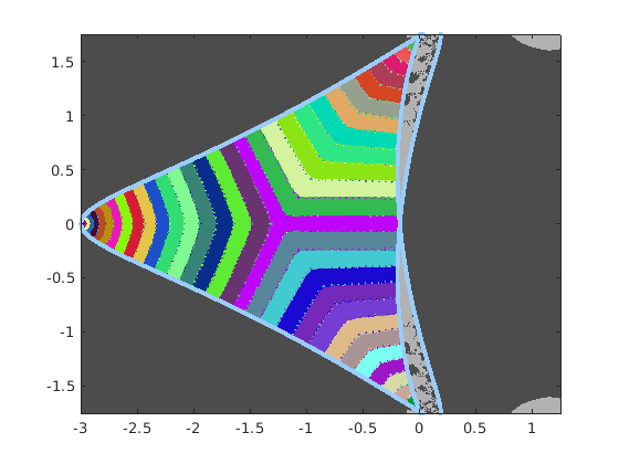
The algorithms have been applied in the double precision floating point arithmetic. The basins of attraction have been constructed as follows. A generic point in the picture, corresponding to the complex number $\lambda_{0}$ has been coloured with a colour depending on the limit of the sequence generated by fixed point iteration $\lambda_{k+1}=g(\lambda_{k})$ for $k\geq 0$. Different colours, randomly generated, have been used for different limits. Different levels of gray have been used to denote that the iteration has been halted with no convergence. The colour green has been used for the values $\lambda_{0}$ belonging to a continuous set of eigenvalues.

The results

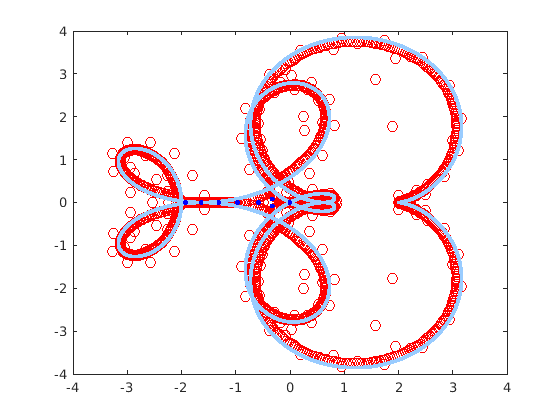
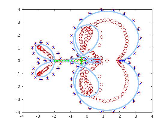
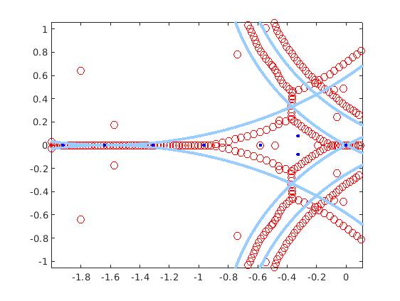
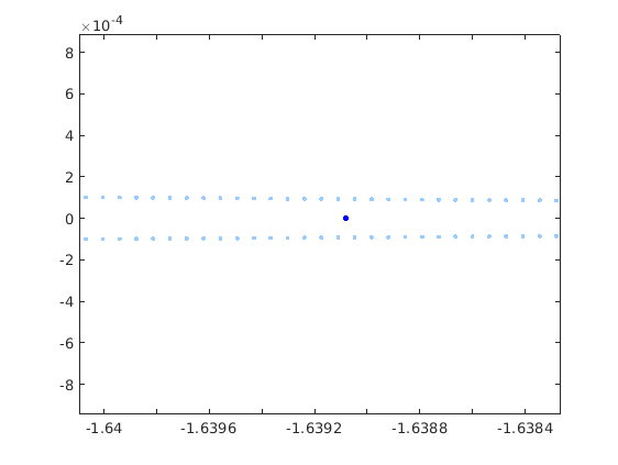
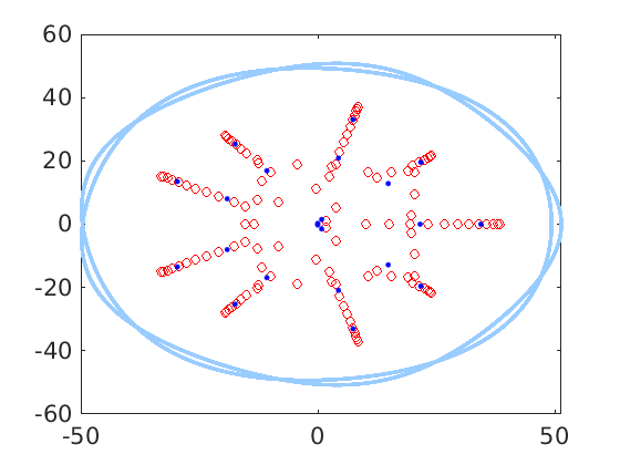
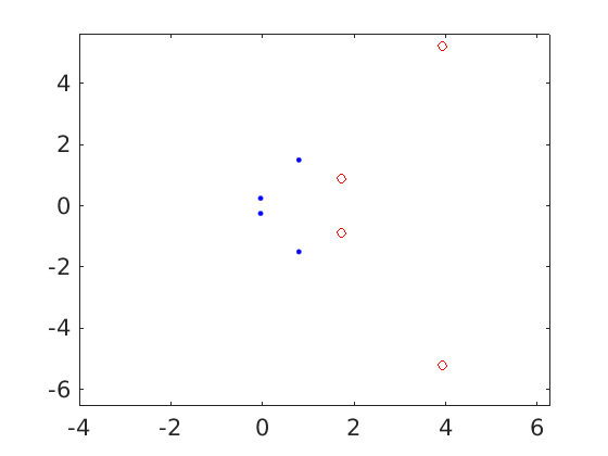
In the figures where the eigenvalues are reported, red circles indicate the eigenvalues of the finite section $A_{N}$, blue dots represent isolated eigenvalues of $A$, while red circles containing a green dot represent eigenvalues of $A_{N}$ that belong to a continuous set of eigenvalues. The light blue curve denotes the set $a(\mathbb{T})$. In the figures displaying the basins of attraction, the light green area indicates a continuous set of eigenvalues. For this set of figures, Algorithm V has been applied.

Figure 3 displays the eigenvalues of $A+E_{1}$, for the matrix of Test 1, and the basins of attraction of Newton’s iteration, together with a zoom of a specific area.

Figure 4 displays the analogous images for the matrix $A+E_{2}$ of Test 1. Here, it is interesting to observe the existence of a connected component formed by a continuous set of eigenvalues denoted by a green triangle-shaped figure. Observe also that the corresponding red circles in this component contain a green dot.

Figure 3: Test 1, Case 1: Eigenvalues of the QT matrix $A$ (blue dots) and of the finite section $A_{N}$ (red circles), together with the basins of attraction for Newton’s iteration computed by Algorithm V. On the right the zoom of a portion.

Figure 4: Test 1, Case 2: Eigenvalues of the QT matrix $A$ (blue dots) and of the finite section $A_{N}$ (red circles), together with the basins of attraction for Newton’s iteration computed by Algorithm V. On the right the zoom of a portion.

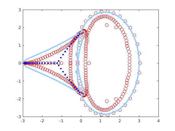
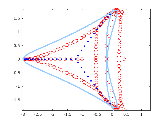
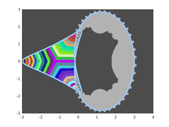
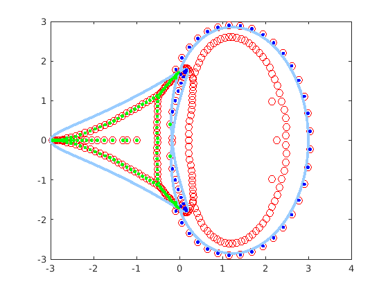
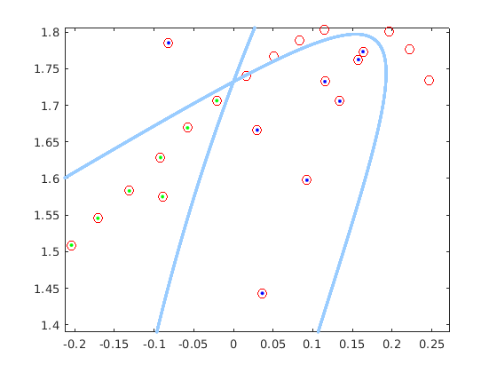
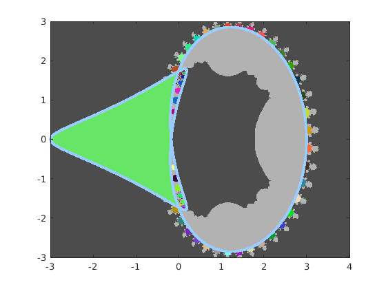
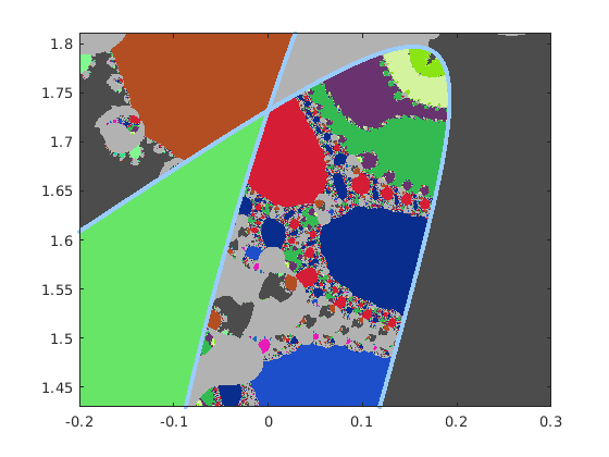
The smallest value of $N_{0}$ for which the number of computed eigenvalues is constant for $N\geq N_{0}$ is $N_{0}=400$ for the Case 1, while it is $N_{0}=200$ for the Case 2. In both cases, the geometry of the basins of attraction, together with the distribution of the eigenvalues of $A_{N}$, explains why Newton’s iteration converges to all the eigenvalues, when starting from the eigenvalues of $A_{N}$ for a quite small value of $N$, even though the latter eigenvalues are far from the eigenvalues of $A$. This latter property is more evident in Case 1, where several blue dots are not contained inside red circles, see Figure 3, zoomed part.

The number of iterations to arrive at convergence is quite small and is the same for both algorithms. Namely, concerning Case 1, it ranges from 3 to 18 with the avergae value of 7.5; concerning Case 2, it ranges from 3 to 10 with average 3.3.

Another interesting issue to investigate, independently of the algorithm used, is to analyze how large must be $N$ in order that the eigenvalues of $A_{N}$ approximate all the eigenvalues of $A$ within the machine precision $u=\tt 2.22e-16$ so that no step of Newton’s iteration would be necessary. It turns out that for the Test 1, Case 1, almost all the eigenvalues are well approximated already for $N=800$, while there are few eigenvalues that require a pretty larger size. Table 1 shows a few significant cases. Typically, the eigenvalues closest to the light blue curve are the ones that need a large value of the truncation level $N$ to be properly approximated by a corresponding eigenvalue of $A_{N}$. For instance, from Table 1 it turns out that $N=3200$ is not enough to approximate the rightmost eigenvalue. Even $N=6400$ does not provide a full accuracy approximation. A similar situation holds for the Case 2.

$\lambda~{}\backslash~{}N$	200	400	800	$1600$	$3200$	$6400$
-4.0e-01$\pm$1.2e+00i	4.1e-04	1.3e-08	–
-3.1e-01$\pm$1.3e+00i	3.0e-03	3.9e-06	5.3e-12	–
-2.2e-01$\pm$1.5e+00i	5.4e-03	6.1e-05	5.9e-09	–
-1.4e-01$\pm$1.6e+00i	2.6e-02	2.0e-03	2.7e-05	1.9e-10	–
-5.9e-02$\pm$1.6e+00i	6.5e-02	3.5e-02	1.1e-02	3.5e-04	9.2e-07	3.8e-13

Table 1: Test1, Case 1: Distances of some eigenvalues of $A$ from the closest eigenvalue of $A_{N}$ for different values of $N$. A “–” denotes a value below 1.e-15.

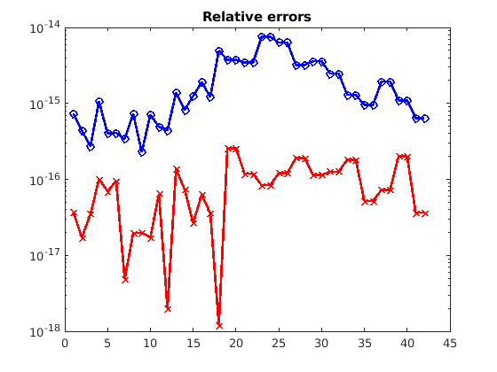
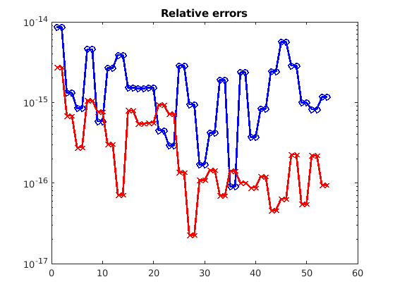
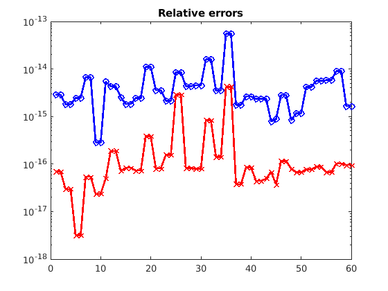
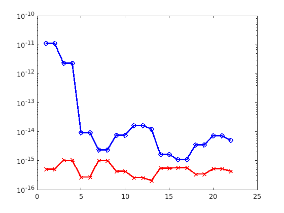
Concerning the accuracy of approximation, Figure 5 shows the relative errors of approximating the eigenvalues of $A$ with the Vandermonde approach (blue circle) and with the Frobenius approach (red cross) in the two cases of Test 1. Here, the eigenvalues have been sorted according to the real part. The relative errors have been obtained by comparing the eigenvalues computed in the standard floating point arithmetic with those computed in the quadruple precision relying on Advanpix. Observe that the results obtained by the Frobenius version are generally more accurate than the ones obtained with the Vandermonde version.

Figure 5: Test 1. Relative errors in each eigenvalue computed with Algorithm V (blue circle) and with Algorithm F (red cross). Case 1 and case 2 on the left and on the right, respectively. Eigenvalues are sorted with respect to the real part.

Finally, concerning the CPU time, the two algorithms have similar performances even though, for this test, Algorithm F generally requires a double time.

Test 2, Case 1, points out in a more evident manner that the eigenvalues of $A$ which are close to the curve $a(\mathbb{T})$ can be hardly approximated by the eigenvalues of a finite section $A_{N}$ of $A$, unless $N$ is extremely large. In fact, as clearly shown in Figure 6 and in the zoomed areas, out of the 8 eigenvalues of $A$, there is a group of few eigenvalues that lie very close to the light blue curve. In particular, the second (from the left) eigenvalue and the last one. The distances of these eigenvalues to the closest eigenvalue of $A_{N}$ for different values of $N$ are reported in Table 2. It turns out that in order to approximate such eigenvalues within the machine precision $u$ without applying Newton’s iteration, one would need truncation levels larger than $1.6$ millions, whereas Newton’s iteration converges quickly just starting from the eigenvalues of $A_{N}$, with $N=3200$.

Figure 6: Test 2, In the first line the eigenvalues of Case 1 (left) and Case 2 (right) are displayed with a blue dot. In the second line, some portion of the domain where the eigenvalues of Case 1 are located are displayed; more specifically, from the left, the area with all the eigenvalues, the second leftmost eigenvalue, and the last rightmost eigenvalue are zoomed, respectively.

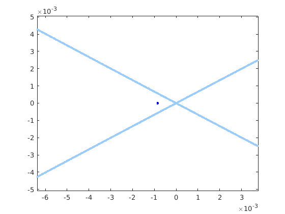
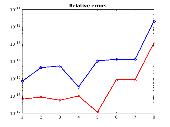
Also in this test, the number of iterations required by Algorithm V and Algorithm F is the same. Namely, for Case 1 it ranges between 5 and 12 with average value 7.25, for Case 2 it ranges between 2 and 4 with average value 3.0. Algorithm F turns out to be more accurate than Algorithm V as shown in Figure 7.

Figure 7: Test 2. Relative errors in each eigenvalue computed with Algorithm V (blue circle) and with Algorithm F (red cross). Case 1 and case 2 on the left and on the right, respectively. Eigenvalues are sorted with respect to the real part.

$\lambda~{}\backslash~{}N$	$400$	$1600$	$6400$	$25600$	$102400$	$409600$	$1638400$
-1.9	1.4e-01	8.3e-02	4.1e-05	–
-1.6	7.6e-01	2.3e-01	9.8e-02	5.8e-02	2.9e-03	2.6e-03	1.4e-07
-1.3	4.2e-01	1.2e-01	1.5e-04	–
-9.6e-01	1.6e-01	5.2e-06	–
-5.8e-01	3.0e-03	7.3e-11	–
-8.5e-04	6.8e-02	1.0e-01	9.2e-02	7.8e-03	2.9e-04	5.3e-13	–

Table 2: Test 2, Case 1: Distances of the real eigenvalues of $A$ from the closest eigenvalue of $A_{N}$ for different values of $N$. A “–” denotes a value below 1.e-15.

Concerning Test 3, the matrix $A$ has a set $\mathcal{S}$ of 22 eigenvalues, shown in Figure 8, that can be grouped into 3 subsets $\mathcal{S}_{1}$, $\mathcal{S}_{2}$, $\mathcal{S}_{3}$. The subset $\mathcal{S}_{1}$ is formed by 4 entries of modulus in the range $[0.25,1.7]$, while $\mathcal{S}_{2}$ and $\mathcal{S}_{3}$ are formed by 9 entries of modulus roughly 20, and 30, respectively. Recall that the Mignotte-like polynomial $z^{m}a(z)$ has a tight cluster formed by three ill-conditioned zeros. For $\lambda\in\mathcal{S}$ the polynomial $z^{m}(a(z)-\lambda)$ still has a cluster of ill-conditioned zeros, where the cluster is tighter and consequently the zeros are more ill-conditioned the smaller is $|\lambda|$. This explains why the errors of the algorithm based on the Vandermonde formulation are much higher in the leftmost part of the graph shown in Figure 8.

Figure 8: Test 3. From the left: Geometry of the eigenvalues with a zoom of the cluster computed by Algorithm F; relative errors for each eigenvalue computed by Algorithm V (blue circle) and by Algorithm F (red cross), where eigenvalues are sorted by increasing modulus.

7 Conclusions and open problems

The problem of computing the eigenvalues of a QT matrix has been reformulated as a nonlinear eigenvalue problem. Newton’s iteration has been analyzed for this task both in the Vandermonde version and in the Frobenius version. As initial approximation for starting the iteration we use the eigenvalues of the truncated matrix $A_{N}$. Numerical experiments show the effectiveness of our approach. The algorithm based on the Frobenius formulation turned out to be more accurate even though slightly slower. Approximating all the eigenvalues to the machine precision directly from the eigenvalues of the truncated matrix $A_{N}$, without using Newton’s iteration, is shown to be infeasible due to the huge values needed for $N$. A Matlab implementation of the algorithm has been provided and the software has been included in the CQT-toolbox of [9].

In order to make the software more robust and effective we plan to provide an optimized implementation of polynomial spectral factorization relying on the algorithms of [14] and [15]. Another important issue is to find theoretical estimates of the truncation parameter $N$ that guarantees the approximation to all the eigenvalues of $A$, starting from those of $A_{N}$. Other approaches to solving the nonlinear eigenvalue problem, say the ones based on rational approximation, could be the subject of subsequent research.

References

- [1] S. Barnett. Polynomials and linear control systems, volume 77 of Monographs and Textbooks in Pure and Applied Mathematics. Marcel Dekker, Inc., New York (1983).
- [2] D. A. Bini, G. Fiorentino, L. Gemignani, and B. Meini. Effective fast algorithms for polynomial spectral factorization. Numer. Algorithms, 34(2-4), 217–227 (2003).
- [3] D. A. Bini, B. Iannazzo, and J. Meng. Algorithms for Approximating Means of Semi-infinite Quasi-Toeplitz Matrices. In B. F. Nielsen F., editor, Geometric Science of Information, GSI 2021, volume 12829 of Lecture Notes in Computer Science, pages 405–414. Springer (2021).
- [4] D. A. Bini, B. Iannazzo, and J. Meng. Geometric means of quasi-Toeplitz matrices. arXiv preprint. (2021).
- [5] D. A. Bini, G. Latouche, and B. Meini. Numerical methods for structured Markov chains. Numerical Mathematics and Scientific Computation. Oxford University Press, New York (2005).
- [6] D. A. Bini, S. Massei, and B. Meini. Semi-infinite quasi-Toeplitz matrices with applications to QBD stochastic processes. Math. Comp., 87(314), 2811–2830 (2018).
- [7] D. A. Bini, S. Massei, B. Meini, and L. Robol. On quadratic matrix equations with infinite size coefficients encountered in QBD stochastic processes. Numer. Linear Algebra Appl., 25(6), 2128, 12 (2018).
- [8] D. A. Bini, S. Massei, B. Meini, and L. Robol. A computational framework for two-dimensional random walks with restarts. SIAM J. Sci. Comput., 42(4), A2108–A2133 (2020).
- [9] D. A. Bini, S. Massei, and L. Robol. Quasi-Toeplitz matrix arithmetic: a MATLAB toolbox. Numerical Algorithms, 81(2), 741–769 (2019).
- [10] D. A. Bini and B. Meini. On the exponential of semi-infinite quasi-Toeplitz matrices. Numer. Math., 141(2), 319–351 (2019).
- [11] D. A. Bini, B. Meini, and J. Meng. Solving quadratic matrix equations arising in random walks in the quarter plane. SIAM J. Matrix Anal. Appl., 41(2), 691–714 (2020).
- [12] A. Böttcher and S. M. Grudsky. Toeplitz matrices, asymptotic linear algebra, and functional analysis. Birkhäuser Verlag, Basel (2000).
- [13] A. Böttcher and S. M. Grudsky. Spectral properties of banded Toeplitz matrices. Society for Industrial and Applied Mathematics (SIAM), Philadelphia, PA (2005).
- [14] A. Böttcher and M. Halwass. A Newton method for canonical Wiener-Hopf and spectral factorization of matrix polynomials. Electron. J. Linear Algebra, 26, 873–897 (2013).
- [15] A. Böttcher and M. Halwass. Wiener-Hopf and spectral factorization of real polynomials by Newton’s method. Linear Algebra Appl., 438(12), 4760–4805 (2013).
- [16] A. Böttcher and B. Silbermann. Introduction to large truncated Toeplitz matrices. Universitext. Springer-Verlag, New York (1999).
- [17] J. P. D’Angelo. Several complex variables and the geometry of real hypersurfaces. Studies in Advanced Mathematics. CRC Press, Boca Raton, FL (1993).
- [18] W. Gander. New algorithms for solving nonlinear eigenvalue problems. Comput. Math. Math. Phys., 61(5), 761–773 (2021).
- [19] C. Garoni and S. Serra-Capizzano. Generalized locally Toeplitz sequences: theory and applications. Vol. I. Springer, Cham (2017).
- [20] C. Garoni and S. Serra-Capizzano. Generalized locally Toeplitz sequences: theory and applications. Vol. II. Springer, Cham (2018).
- [21] B. Gavin, A. Miedlar, and E. Polizzi. FEAST eigensolver for nonlinear eigenvalue problems. J. Comput. Sci., 27, 107–117 (2018).
- [22] S. Güttel and F. Tisseur. The nonlinear eigenvalue problem. Acta Numer., 26, 1–94 (2017).
- [23] M. E. Hochstenbach and B. Plestenjak. Computing several eigenvalues of nonlinear eigenvalue problems by selection. Calcolo, 57(2), Paper No. 16, 25 (2020).
- [24] J. R. Jackson. Networks of waiting lines. Operations Res., 5, 518–521 (1957).
- [25] H.-M. Kim and J. Meng. Structured perturbation analysis for an infinite size quasi-Toeplitz matrix equation with applications. BIT Numerical Mathematics, 61, 859–879 (2021).
- [26] G. Latouche and V. Ramaswami. Introduction to matrix analytic methods in stochastic modeling. ASA-SIAM Series on Statistics and Applied Probability. SIAM, Philadelphia, PA (1999).
- [27] M. Mignotte. Some useful bounds. In Computer algebra, pages 259–263. Springer, Vienna (1983).
- [28] M. F. Neuts. Matrix-geometric solutions in stochastic models: An algorithmic approach, volume 2 of Johns Hopkins Series in the Mathematical Sciences. Johns Hopkins University Press, Baltimore, Md. (1981).
- [29] A. Ostrowski. Recherches sur la méthode de Graeffe et les zéros des polynomes et des séries de Laurent. Acta Mathematica, 72, 99 – 155 (1940).
- [30] T. Ozawa. Stability condition of a two-dimensional qbd process and its application to estimation of efficiency for two-queue models. Performance Evaluation, 130, 101 – 118 (2019).
- [31] T. Ozawa. Asymptotic properties of the occupation measure in a multidimensional skip-free Markov-modulated random walk. Queueing Syst., 97(1-2), 125–161 (2021).
- [32] L. Robol. Rational Krylov and ADI iteration for infinite size quasi-Toeplitz matrix equations. Linear Algebra Appl., 604, 210–235 (2020).
- [33] M. Schechter. Basic theory of Fredholm operators. Ann. Scuola Norm. Sup. Pisa Cl. Sci. (3), 21:261–280 (1967).