Low-Complexity Multicast Beamforming for Millimeter Wave Communications

Abstract

To develop a low-complexity multicast beamforming method for millimeter wave communications, we first propose a channel gain estimation method in this article. We use the beam sweeping to find the best codeword and its two neighboring codewords to form a composite beam. We then estimate the channel gain based on the composite beam, which is computed off-line by minimizing the variance of beam gain within beam coverage. With the estimated channel gain, we propose a multicast beamforming design method under the max-min fair (MMF) criterion. To reduce the computational complexity, we divide the large antenna array into several small-size sub-arrays, where the size of each sub-array is determined by the estimated channel gain. In particular, we introduce a phase factor for each sub-array to explore additional degree of freedom for the considered problem. Simulation results show that the proposed multicast beamforming design method can substantially reduce the computational complexity with little performance sacrifice compared to the existing methods.

I Introduction

Millimeter wave (mmWave) communication is a promising technology for the next generation wireless systems due to its large bandwidth and high achievable rate [1]. However, much smaller number of radio-frequency (RF) chains than the number of antennas are used in mmWave communications to save the hardware cost [2]. To serve more users with limited RF chains, we consider mmWave multicast, which can simultaneously transmit common message to multiple users. Since the mmWave communications need highly directional beamforming [3], the design of mmWave multicast beamforming is on focus.

There have been two criteria for multicast beamforming design in the literature. One aims at minimizing the total transmit power under a predefined signal-to-noise-ratio (SNR) constraint of each user, which is named as quality of service (QoS) criterion. The other aims to maximize the minimum SNR of all users under the total transmit power constraint, which is named as max-min fair (MMF) criterion. Both criteria result in NP-hard optimization problems. Therefore, they are tackled by interior point methods based on semi-definite relaxation under full-digital beamforming structure (SDR-FD) [4]. To reduce the complexity of SDR-FD, the full-digital beamformer is divided into an outer-layer and an inner-layer beamformer, where the former is used to remove multigroup interference and the latter is used to solve the original problems via successive convex approximation [5]. Another way to reduce the complexity of SDR-FD is to approximate the original problem by a sequence of convex subproblems via convex-concave procedures, where each subproblem is then solved by alternating direction method of multipliers [6]. Note that these works are for the full-digital beamforming structure and not applicable for mmWave communications. In [7], mmWave analog beamforming is designed by alternatively optimizing each entry of the beamformer (ALTER) based on the MMF criterion. However, the assumption of perfect channel state information (CSI) is sometimes impractical and the computational complexity of ALTER is high.

In this work, we reduce the design complexity of mmWave multicast beamforming based on the estimated CSI. The contribution of this work can be summarized as follows.

1) We develop a channel gain estimation method. We first use the beam sweeping to find the best codeword, whose two neighboring codewords are used to perform additional beam training. Then we estimate the channel gain based on the composite beam, which is computed off-line by minimizing the variance of beam gain within beam coverage.

2) We propose a multicast beamforming design method under the MMF criterion. To reduce the computational complexity, we divide the large antenna array into several small-size sub-arrays, where the size of each sub-array is determined by the estimated channel gain. In particular, we introduce a phase factor for each sub-array to explore additional degree of freedom for the considered problem.

Notations: Symbols for matrices (upper case) and vectors (lower case) are in boldface. $(\cdot)^{\ast}$, $(\cdot)^{\rm T}$, $(\cdot)^{\rm H}$, $\mathbb{E}\{\cdot\}$, $\rm var(\cdot)$, $\rm round(\cdot)$ and $\mathcal{CN}$ denote the conjugate, transpose, Hermitian (conjugate transpose), expectation, variance, round operation and complex Gaussian distribution, respectively. $\angle(a)$ and $|a|$ denote the angle and amplitude of a complex number $a$, respectively. $\boldsymbol{a}[i]$ denotes the $i$th entry of a vector $\boldsymbol{a}$.

II System Model

Consider an mmWave multicast system with $N_{\rm BS}$ antennas at the base station (BS) and $K$ single-antenna users. The antennas at the BS are placed in a uniform linear array (ULA) with a half wavelength interval. Let $s$ denote the transmitted symbol with unit power, i.e., $\mathbb{E}\{|s|^{2}\}=1$. Then the received signal at the $k$th user for $k=1,2,\ldots,K$ is

$$y_{k}=\sqrt{P}\boldsymbol{h}^{\rm H}_{k}\boldsymbol{f}_{\rm RF}s+n_{k}$$ (1)

where $P$, $\boldsymbol{f}_{\rm RF}$, $\boldsymbol{h}_{k}$, and $n_{k}$ denote the total power of the transmitter, analog beamforming vector, mmWave channel vector, and additive white Gaussian noise (AWGN) obeying $n_{k}\thicksim\mathcal{CN}(0,\sigma_{k}^{2})$, respectively. According to the widely used Saleh-Valenzuela mmWave channel model [8], the channel vector between the BS and the $k$th user can be expressed as

$$\boldsymbol{h}_{\emph{k}}=\sqrt{N_{\rm BS}}\Big{(}\alpha_{k}\boldsymbol{u}(N_{\rm BS},\varphi_{k})+\sum_{l=1}^{L}\alpha_{k}^{(l)}\boldsymbol{u}(N_{\rm BS},\varphi_{k}^{(l)})\Big{)}$$ (2)

where $\alpha_{k}$ and $\varphi_{k}$ denote the channel coefficient and the channel angle of departure (AoD) of the line-of-sight (LoS) path, respectively; and $\alpha_{k}^{(l)}$ and $\varphi_{k}^{(l)}$ denote the channel coefficient and the channel AoD of the $l$th non-line-of-sight (NLoS) paths, respectively, for $l=1,2,\ldots,L$. The channel steering vector is defined as a function of $N$ and $\varphi$ as

$$\boldsymbol{u}(N,\varphi)=\frac{1}{\sqrt{N}}[1,e^{j\pi\varphi},...,e^{j(N-1)\pi\varphi}]^{\rm T}$$ (3)

where $N$ and $\varphi$ are the number of BS antennas and the channel AoD, respectively.

III Channel Gain Estimation

Suppose we perform the beam sweeping simultaneously for all $K$ users based on a predefined codebook

$$\boldsymbol{\mathcal{F}}_{c}\triangleq\{\boldsymbol{f}_{1},\boldsymbol{f}_{2},...,\boldsymbol{f}_{N_{\rm BS}}\},$$ (4)

where

$$\boldsymbol{f}_{n}\triangleq\boldsymbol{u}(N_{\rm BS},-1+(2n-1)/N_{\rm BS})$$ (5)

is the $n$th codeword with beam coverage of $[-1+2(n-1)/N_{\rm BS},-1+2n/N_{\rm BS}]$. The $k$th user finds the index of its best codeword by

$$J_{k}=\arg\max_{i}\big{|}\sqrt{P}\boldsymbol{h}^{\rm H}_{k}\boldsymbol{f}_{i}s+n_{k}\big{|},~{}k=1,2,\ldots,K.$$ (6)

The received signal by the $k$th user corresponding to the best codeword is

$$y_{k}^{\rm C} \triangleq\sqrt{P}\boldsymbol{h}^{\rm H}_{k}\boldsymbol{f}_{J_{k}}s+n_{k}^{\rm C}.$$ (7)

In fact that the beam gain of $\boldsymbol{f}_{J_{k}}$ on NLoS paths is much smaller than that on the LoS path, we can obtain the approximation in (7) as

$$y_{k}^{\rm C}\approx\sqrt{PN_{\rm BS}}\big{(}\alpha_{k}\boldsymbol{u}(N_{\rm BS},\varphi_{k})\big{)}^{\rm H}\boldsymbol{f}_{J_{k}}s+n_{k}^{\rm C}.$$ (8)

Then the estimated channel AoD corresponding to the channel LoS path is

$$\widehat{\varphi}_{k}\triangleq-1+(2J_{k}-1)/N_{\rm BS},$$ (9)

which is inaccurate since any genuine channel AoD in $[\widehat{\varphi}_{k}-\frac{1}{N_{\rm BS}},\widehat{\varphi}_{k}+\frac{1}{N_{\rm BS}}]$ will all result in the estimated channel AoD of $\widehat{\varphi}_{k}$ due to the limited resolution of $\boldsymbol{\mathcal{F}}_{c}$. As a consequence, the channel gain estimation is not accurate enough.

To improve the channel gain estimation, we perform additional two beam training tests. Denote the left and right neighbouring codewords of $\boldsymbol{f}_{J_{k}}$ as $\boldsymbol{f}_{J_{k}}^{\rm L}$ and $\boldsymbol{f}_{J_{k}}^{\rm R}$, respectively, where

$$\boldsymbol{f}_{J_{k}}^{\rm L}\triangleq\boldsymbol{u}(N_{\rm BS},\widehat{\varphi}_{k}-\frac{2}{N_{\rm BS}}),$$ (10)

$$\boldsymbol{f}_{J_{k}}^{\rm R}\triangleq\boldsymbol{u}(N_{\rm BS},\widehat{\varphi}_{k}+\frac{2}{N_{\rm BS}}).$$ (11)

Similar to (8), we can approximate the received signal as

$$y_{k}^{\rm L}\approx\sqrt{PN_{\rm BS}}\big{(}\alpha_{k}\boldsymbol{u}(N_{\rm BS},\varphi_{k})\big{)}^{\rm H}\boldsymbol{f}_{J_{k}}^{\rm L}s+n_{k}^{\rm L},$$ (12)

$$y_{k}^{\rm R}\approx\sqrt{PN_{\rm BS}}\big{(}\alpha_{k}\boldsymbol{u}(N_{\rm BS},\varphi_{k})\big{)}^{\rm H}\boldsymbol{f}_{J_{k}}^{\rm R}s+n_{k}^{\rm R}.$$ (13)

Algorithm 1 Channel Gain Estimation

1:  Input: $N_{\rm BS}$, $\{\boldsymbol{h}_{k},k=1,2,\ldots,K\}$.

2:  Obtain $\widetilde{\eta}_{1}$ and $\widetilde{\eta}_{2}$ via (16).

3:  Compute $Z$ via (17).

4:  Perform beam sweeping to obtain $J_{k}$ and $y_{k}^{\rm C}$ via (6) and (7), respectively.

5:  Obtain the estimated channel AoD $\widehat{\varphi}_{k}$ via (9).

6:  Perform additional beam training to obtain $y_{k}^{\rm L}$ and $y_{k}^{\rm R}$ via (12) and (13), respectively.

7:  Estimate the channel gain $\big{|}\widehat{\alpha}_{k}\big{|}$ via (18).

8:  Output: $\{\big{|}\widehat{\alpha}_{k}\big{|},k=1,2,\ldots,K\}$.

We introduce two phase variables, $\eta_{1},\eta_{2}\in(-\pi,\pi]$ to combine the received signals in (12) and (13) together with (8) by

$$y_{k}^{\rm com}\triangleq y_{k}^{\rm C}+e^{j\eta_{1}}y_{k}^{\rm L}+e^{j\eta_{2}}y_{k}^{\rm R}\approx\sqrt{P}\alpha_{k}^{\ast}g(\varphi_{k},\eta_{1},\eta_{2})s$$ (14)

where

$$g(\varphi_{k},\eta_{1},\eta_{2})\triangleq\sqrt{N_{\rm BS}}\boldsymbol{u}(N_{\rm BS},\varphi_{k})^{\rm H}(\boldsymbol{f}_{J_{k}}^{\rm C}+e^{j\eta_{1}}\boldsymbol{f}_{J_{k}}^{\rm L}+e^{j\eta_{2}}\boldsymbol{f}_{J_{k}}^{\rm R})$$ (15)

denotes the composite beam gain of the three codewords. The motivation to introduce $\eta_{1}$ and $\eta_{2}$ is to make $g(\varphi,\eta_{1},\eta_{2})$ almost constant within the beam coverage $\varphi\in[\widehat{\varphi}_{k}-\frac{2}{N_{\rm BS}},\widehat{\varphi}_{k}+\frac{2}{N_{\rm BS}}]$ by exploring additional degree of freedom of $\eta_{1}$ and $\eta_{2}$, so that we can estimate the channel gain $|\alpha_{k}|$ accurately based on (14). To this end, we choose $\eta_{1}$ and $\eta_{2}$ to minimize the variance of $g(\varphi,\eta_{1},\eta_{2})$ for $\varphi\in[\widehat{\varphi}_{k}-\frac{2}{N_{\rm BS}},\widehat{\varphi}_{k}+\frac{2}{N_{\rm BS}}]$, which can be expressed as

$$[\widetilde{\eta}_{1},\widetilde{\eta}_{2}]=\arg\min_{\eta_{1},\eta_{2}\in[-\pi,\pi]}{\rm var}\big{(}g(\varphi,\eta_{1},\eta_{2})\big{)}.$$ (16)

The optimization problem of (16) can be solved using the existing methods [9]. In fact, $\widetilde{\eta}_{1}$ and $\widetilde{\eta}_{2}$ can be computed off-line before the beam sweeping since different $\widehat{\varphi}_{k}$ only changes the center of the composite beam without any change of the composite beam pattern. Without loss of generality, the first three neighbouring codewords $\boldsymbol{f}_{1}$, $\boldsymbol{f}_{2}$, and $\boldsymbol{f}_{3}$ in $\boldsymbol{\mathcal{F}}_{c}$ are used to compute $\widetilde{\eta}_{1}$ and $\widetilde{\eta}_{2}$, where $\widehat{\varphi}_{k}=-1+3/N_{\rm BS}$. We define

$$Z\triangleq\frac{1}{Q}\sum_{q=1}^{Q}\Big{|}g\big{(}-1+\frac{1}{N_{\rm BS}}+\frac{4q}{N_{\rm BS}Q},\widetilde{\eta}_{1},\widetilde{\eta}_{2}\big{)}\Big{|}.$$ (17)

where we equally sample $[-1+\frac{1}{N_{\rm BS}},-1+\frac{5}{N_{\rm BS}}]$ by $Q$ points. As $Q$ grows to be infinity, $Z$ will approach the mean of $\big{|}g(\varphi,\widetilde{\eta}_{1},\widetilde{\eta}_{2})\big{|}$ for $\varphi\in[-1+\frac{1}{N_{\rm BS}},-1+\frac{5}{N_{\rm BS}}]$.

Then the channel gain estimation can be obtained by

$$\big{|}\widehat{\alpha}_{k}\big{|}=\bigg{|}\frac{y_{k}^{\rm C}+e^{j\widetilde{\eta}_{1}}y_{k}^{\rm L}+e^{j\widetilde{\eta}_{2}}y_{k}^{\rm R}}{sZ\sqrt{P}}\bigg{|}.$$ (18)

where $\widehat{\alpha}_{k}$ is an estimate of $\alpha_{k}$.

The steps of the proposed method for channel gain estimation are summarized in Algorithm 1.

IV Low-Complexity Multicast Beamforming

Based on the estimated channel gain as well as the estimated channel AoD, we can design the multicast beamforming so that the BS can simultaneously transmit the same signal to $K$ users.

IV-A Max-Min Fair Problem Formulation

One important metric of multicast beamforming is the user fairness, which maximizes the minimum received SNR for the served users. We formulate the multicast beamforming design problem under the MMF criterion as

$$\max_{\boldsymbol{f}_{\rm RF}}\min_{k=1,2,...,K} \frac{|\boldsymbol{h}_{k}^{\rm H}\boldsymbol{f}_{\rm RF}|^{2}P}{{\sigma}^{2}_{k}}$$ (19a)

$${\rm s.t.}~{}~{}~{}~{}~{}~{}~{}~{}~{}~{}~{}~{}~{} \angle\big{(}\boldsymbol{f}_{\rm RF}[i]\big{)}\in\mathcal{S},~{}i=1,2,\ldots,N_{\rm BS}$$ (19b)

$$|\boldsymbol{f}_{\rm RF}[i]|=\frac{1}{\sqrt{N_{\rm BS}}}$$ (19c)

where $\mathcal{S}$ denotes a set of quantized angles determined by the resolution of phase shifters [10]. We set

$$\mathcal{S}=\{\pi(-1+\frac{2n-1}{N_{\rm BS}}),~{}n=1,2,\ldots,N_{\rm BS}\},$$ (20)

where the resolution of the phase shifters is $B=\log_{2}{N_{\rm BS}}$. The optimization problem in (19) is a non-convex NP-hard problem. Although we may exhaustively search all available candidates to find the best $\boldsymbol{f}_{\rm RF}$, the computational complexity is prohibitively high, especially when $N_{\rm BS}$ is large. In this context, we consider to divide the large antenna array into $K$ small-size antenna sub-arrays. Denote $N_{k}$ as the size of the $k$th sub-arrays for $k=1,2,\ldots,K$, where

$$N_{1}+N_{2}+\cdots+N_{K}=N_{\rm BS}.$$ (21)

We use $K$ beamforming vectors $\boldsymbol{w}_{1},~{}e^{j{\theta}_{1}}\boldsymbol{w}_{2},\ldots,~{}e^{j{\theta}_{K-1}}\boldsymbol{w}_{K}$ to form analog beams pointing at all the $K$ users, respectively. Based on the estimated channel AoD from (9), we set

$$\boldsymbol{w}_{k}=\frac{1}{\sqrt{N_{\rm BS}}}\big{[}1,e^{j\pi\widehat{\varphi}_{k}},\ldots,e^{j(N_{k}-1)\pi\widehat{\varphi}_{k}}\big{]}^{\rm T}.$$ (22)

Note that we introduce phase factors $\{\theta_{1},\theta_{2},\ldots,\theta_{K-1}\}$ to explore additional degree of freedom to solve (19). Therefore we have

$$\boldsymbol{f}_{\rm RF}=[\boldsymbol{w}_{1}^{\rm T},e^{j{\theta}_{1}}\boldsymbol{w}_{2}^{\rm T},\ldots,e^{j{\theta}_{K-1}}\boldsymbol{w}_{K}^{\rm T}]^{\rm T}$$ (23)

which converts the optimization of $\boldsymbol{f}_{\rm RF}$ into the optimization of $\{\theta_{1},\theta_{2},\ldots,\theta_{K-1}\}$ and $\{N_{1},N_{2},\ldots,N_{K}\}$.

IV-B Determination of Sub-Array Size

Based on Lemma 2 in [11], the optimal solution of the MMF problem in (19) can be obtained when all users have the same SNR, which can be expressed as

$${\frac{|\boldsymbol{h}_{1}^{\rm H}\boldsymbol{f}_{\rm RF}|^{2}P}{{\sigma}_{1}^{2}}}={\frac{|\boldsymbol{h}_{2}^{\rm H}\boldsymbol{f}_{\rm RF}|^{2}P}{{\sigma}_{2}^{2}}}=\cdots={\frac{|\boldsymbol{h}_{K}^{\rm H}\boldsymbol{f}_{\rm RF}|^{2}P}{{\sigma}_{K}^{2}}}.$$ (24)

Since the mmWave analog beamforming is highly directional, the beam gain for the $k$th user mainly comes from the $k$th sub-array. Therefore, we define a zero vector $\overline{\boldsymbol{w}}_{k}$ with the length of $N_{\rm BS}$, except that the entries corresponding to the $k$th sub-array are set the same as $\boldsymbol{w}_{k}$. Then we set

$${\frac{|\boldsymbol{h}_{1}^{\rm H}\overline{\boldsymbol{w}}_{1}|^{2}}{{\sigma}^{2}_{1}}}={\frac{|\boldsymbol{h}_{2}^{\rm H}\overline{\boldsymbol{w}}_{2}|^{2}}{{\sigma}^{2}_{2}}}=\cdots={\frac{|\boldsymbol{h}_{K}^{\rm H}\overline{\boldsymbol{w}}_{K}|^{2}}{{\sigma}^{2}_{K}}}$$ (25)

to approximate (24). Note that in practice $\boldsymbol{h}_{1},\boldsymbol{h}_{2},\ldots,\boldsymbol{h}_{K}$ cannot be directly obtained. Instead, we use beam sweeping to obtain an estimate of $\boldsymbol{h}_{k}$ as

$$\widehat{\boldsymbol{h}}_{k}=\widehat{\alpha}_{k}\boldsymbol{u}(N_{\rm BS},\widehat{\varphi}_{k}).$$ (26)

Substituting (26) into (25), we have

$$\frac{|\widehat{\alpha}_{1}|N_{1}}{\sigma_{1}}=\frac{|\widehat{\alpha}_{2}|N_{2}}{\sigma_{2}}=\cdots=\frac{|\widehat{\alpha}_{K}|N_{K}}{\sigma_{K}}.$$ (27)

Based on (21) and (27), we can determine $N_{k}$ by

$$N_{k}=\left\{\begin{array}[]{cl}{\rm round}\Big{(}\frac{\sigma_{k}N_{\rm BS}}{{|\widehat{\alpha}_{k}|}\sum_{l=1}^{K}{\sigma_{l}/{|\widehat{\alpha}_{l}|}}}\Big{)},&k=1,2,...,K-1,\\ N_{\rm BS}-\sum_{k=1}^{K-1}N_{k},&k=K.\end{array}\right.$$ (28)

Then $\boldsymbol{w}_{k}$, for $k=1,2,\ldots,K$, can be determined by (22).

In fact, we first sort $\{\widehat{\varphi}_{k},k=1,2,\ldots,K\}$ in ascending order, based on which we then divide the large antenna array into the sub-arrays. If the estimated channel AoDs of some users happen to be the same, we combine their sub-arrays together as a single sub-array.

Algorithm 2 Low Complexity Multicast Beamforming Design

1:  Input: $\{\big{|}\widehat{\alpha}_{k}\big{|},k=1,2,\ldots,K\}$, $I_{\rm max}$.

2:  Initialization: $\theta_{n}\leftarrow 0$, $n=1,2,\ldots,K-1$.

3:  Determine $\{N_{k},k=1,2,\ldots,K\}$ via (28).

4:  Set $i\leftarrow 1$, $\gamma\leftarrow 0$.

5:  while $i\leq I_{\rm max}$  do

6:     for $n=1:K-1$ do

7:        Obtain $\widetilde{\theta}_{n}$ via (33).

8:     end for

9:     if $r(\widetilde{\theta}_{1},\widetilde{\theta}_{2},\ldots,\widetilde{\theta}_{K-1})>\gamma$ then

10:        $\gamma\leftarrow r(\widetilde{\theta}_{1},\widetilde{\theta}_{2},\ldots,\widetilde{\theta}_{K-1})$.

11:     else

12:        break.

13:     end if

14:     $i\leftarrow i+1$.

15:  end while

16:  Obtain $\boldsymbol{f}_{\rm RF}$ via (23).

17:  Output: $\boldsymbol{f}_{\rm RF}$.

IV-C Determination of Phase Factors

Once the numbers of sub-array antennas are determined, the multicast beamforming only involves the phase factors according to (23). Then (19) can be converted into

$$\max_{{\theta}_{1},{\theta}_{2},...,{\theta}_{K-1}}\min_{k=1,2,...,K} \frac{|\widehat{\boldsymbol{h}}_{k}^{\rm H}\boldsymbol{f}_{\rm RF}|^{2}P}{{\sigma}^{2}_{k}}$$ (29a)

$${\rm s.t.}~{}~{}~{}~{}~{}~{}~{}~{}~{}~{}~{}~{}~{}~{}~{}~{}~{} {\theta}_{n}\in\mathcal{T},~{}n=1,2,\ldots,K-1,$$ (29b)

where

$$\mathcal{T}\triangleq\{\pi(-1+\frac{2m-1}{2^{M}}),m=1,...,2^{M}\}$$ (30)

denotes a set of quantized angles. In fact, we may set $M\leq B$ to reduce the search space and the computational complexity.

We define

$$r(\theta_{1},\theta_{2},\ldots,\theta_{K-1})\triangleq\min_{k=1,2,...,K}\frac{|\widehat{\boldsymbol{h}}_{k}^{\rm H}\boldsymbol{f}_{\rm RF}|^{2}P}{{\sigma}^{2}_{k}}.$$ (31)

Then (29) can be rewritten as

$$\max_{\theta_{1},\theta_{2},\ldots,\theta_{K-1}\in\mathcal{T}}~{}r(\theta_{1},\theta_{2},\ldots,\theta_{K-1}).$$ (32)

Since the joint optimization of $\theta_{1},\theta_{2},\ldots,\theta_{K-1}$ is difficult to handle, we resort to sequential optimization of $\theta_{1},\theta_{2},\ldots,\theta_{K-1}$, which only optimizes one of $\theta_{1},\theta_{2},\ldots,\theta_{K-1}$ with the others fixed. When optimizing $\theta_{n}$, (32) can be formulated as

$$\widetilde{\theta}_{n}=\arg\max_{\theta_{n}\in\mathcal{T}}~{}r(\theta_{1},\theta_{2},\ldots,\theta_{K-1}).$$ (33)

We sequentially optimize $\theta_{n},n=1,2,\ldots,K-1$ and then obtain $r(\widetilde{\theta}_{1},\widetilde{\theta}_{2},\ldots,\widetilde{\theta}_{K-1})$. We repeat the sequential optimization until we reach a predefined maximum number of iterations $I_{\rm max}$ or $r(\widetilde{\theta}_{1},\widetilde{\theta}_{2},\ldots,\widetilde{\theta}_{K-1})$ cannot increase anymore, which is indicated by step 5 or step 12, respectively.

The steps of the proposed multicast beamforming design method are summarized in Algorithm 2. Note that the output of Algorithm 1, i.e., $\{\big{|}\widehat{\alpha}_{k}\big{|},k=1,2,\ldots,K\}$, is the input of Algorithm 2, which means that Algorithm 1 and Algorithm 2 are in cascade.

IV-D Complexity Analysis

The complexity of Algorithm 2 is $\mathcal{O}\big{(}2^{M}(K-1)I_{\rm max}\big{)}$. As a comparison, the complexity of SDR-FD with constant amplitude (SDR-CA) and ALTER is $\mathcal{O}(N_{\rm BS}^{6})$ and $\mathcal{O}(N^{2}_{\rm BS}KN_{\rm iter})$, respectively, where $N_{\rm iter}$ is the number of iterations for ALTER to converge and is generally set between 2 and 5 [7].

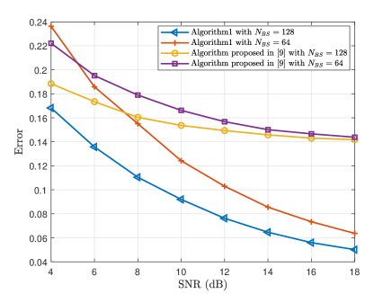
Figure 1: Comparisons of estimation errors for channel gain.

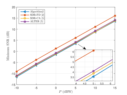
Figure 2: Comparisons of minimum SNR.

V Simulation Results

The considered mmWave multicast system includes a BS equipped with $N_{\rm BS}$ antennas and $K=3$ single-antenna users. The mmWave channel is modeled with one LoS path and $L=2$ NLoS paths, where $\alpha_{k}\thicksim\mathcal{CN}(0,1)$, $\alpha_{k}^{(1)}\thicksim\mathcal{CN}(0,0.01)$ and $\alpha_{k}^{(2)}\thicksim\mathcal{CN}(0,0.01)$. The power of the Gaussian noise is assumed to be $\sigma_{k}^{2}=1$ for $k=1,2,3$. We set $Q=4000$.

We first evaluate the estimation of the channel gain. As shown in Fig. 1, we compare Algorithm 1 with the algorithm proposed in [12], where the estimation error is defined as $\frac{1}{K}\sum_{k=1}^{K}\big{|}|\widehat{\alpha}_{k}|-|\alpha_{k}|\big{|}/|\alpha_{k}|$. We can see that Algorithm 1 outperforms the algorithm proposed in [12]. In particular, the performance gap will get larger as the SNR increases. With larger $N_{\rm BS}$, Algorithm 1 can converge faster. At $\rm{SNR}=18$ dB, the estimation error of Algorithm 1 is only 5%.

Then we evaluate the performance in terms of the minimum SNR. As shown in Fig. 2, we compare Algorithm 2 with SDR-FD [4], SDR-CA and ALTER [7]. We set $N_{\rm BS}=64$, $B=6$, $M=4$ and $I_{\rm max}=30$. Even if the full-digital beamforming is impractical, the performance of SDR-FD can be regarded as the upper bound. We can see that Algorithm 2, ALTER and SDR-CA can all approach the performance of SDR-FD. Although Algorithm 2 is 0.4dB and 0.7dB worse than SDR-CA and ALTER in performance, respectively, its computational complexity is much lower than the other two. According to Section IV-D, the numbers of iterations are 960, 24576 and $64^{6}$ for Algorithm 2, ALTER and SDR-CA, respectively, which indicates Algorithm 2 can reduce the computational complexity by $96.09\%$ and $99.99\%$ compared to ALTER and SDR-CA, respectively.

VI Conclusions

In this article, we have develop a channel gain estimation method, based on which we have proposed a multicast beamforming design method under the MMF criterion. Simulation results have shown that the proposed multicast beamforming design method can substantially reduce the computational complexity with little performance sacrifice compared to the existing methods. Future research includes developing algorithms for simultaneous multiuser beam training to improve the efficiency as well as reducing the overhead of beam training.

References

• [1] L. Yang, Y. Zeng, and R. Zhang, “Channel estimation for millimeter-wave MIMO communications with lens antenna arrays,” IEEE Trans. Veh. Technol., vol. 67, no. 4, pp. 3239–3251, Apr. 2018.
• [2] B. Wang, F. Gao, S. Jin, H. Lin, and G. Y. Li, “Spatial- and Frequency- Wideband Effects in Millimeter-Wave Massive MIMO Systems,” IEEE Trans. Signal Process., vol. 66, no. 13, pp. 3393–3406, July 2018.
• [3] W. Ma, C. Qi, Z. Zhang, and J. Cheng, “Sparse channel estimation and hybrid precoding using deep learning for millimeter wave massive MIMO,” IEEE Trans. Commun., vol. 68, no. 5, pp. 2838–2849, May. 2020.
• [4] N. D. Sidiropoulos, T. N. Davidson, and Z.-Q. Luo, “Transmit beamforming for physical-layer multicasting,” IEEE Trans. Signal Process., vol. 54, no. 6, pp. 2239–2251, June 2006.
• [5] M. Sadeghi, L. Sanguinetti, R. Couillet, and C. Yuen, “Reducing the computational complexity of multicasting in large-scale antenna systems,” IEEE Trans. Wireless Commun., vol. 16, no. 5, pp. 2963–2975, May. 2017.
• [6] E. Chen and M. Tao, “ADMM-based fast algorithm for multi-group multicast beamforming in large-scale wireless systems,” IEEE Trans. Commun., vol. 65, no. 6, pp. 2685–2698, June 2017.
• [7] Z. Wang, Q. Liu, M. Li, and W. Kellerer, “Energy efficient analog beamformer design for mmWave multicast transmission,” IEEE Trans. Green Commun. Netw., vol. 3, no. 6, pp. 552–564, June 2019.
• [8] F. Dong, W. Wang, and Z. Wei, “Low-complexity hybrid precoding for multi-user mmWave systems with low-resolution phase shifters,” IEEE Trans. Veh. Technol., vol. 68, no. 10, pp. 9774–9784, Oct. 2019.
• [9] S. Noh, M. D. Zoltowski, and D. J. Love, “Multi-resolution codebook and adaptive beamforming sequence design for millimeter wave beam aligment,” IEEE Trans. Wireless Commun., vol. 16, no. 9, pp. 5689–5701, Sep. 2017.
• [10] K. Chen, C. Qi, and G. Y. Li, “Two-step codeword design for millimeter wave massive MIMO systems with quantized phase shifters,” IEEE Trans. Signal Process., vol. 68, no. 1, pp. 170–180, Jan. 2020.
• [11] Z. Xiang, M. Tao, and X. Wang, “Massive MIMO multicasting in noncooperative cellular networks,” IEEE J. Sel. Areas Commun., vol. 32, no. 6, pp. 1180–1193, June 2014.
• [12] Z. Xiao, P. Xia, and X.-G. Xia, “Channel estimation and hybrid precoding for millimeter-wave MIMO system: A low-complexity overall solution,” IEEE Access, vol. 5, pp. 16 100–16 110, July 2017.