Doubly Coupled Designs for Computer Experiments

with both Qualitative and Quantitative Factors

Feng Yang, C. Devon Lin, Yongdao Zhou and Yuanzhen He

Sichuan Normal University, Queen’s University, Nankai University

and Beijing Normal University

Abstract: Computer experiments with both qualitative and quantitative input variables occur frequently in many scientific and engineering applications. How to choose input settings for such experiments is an important issue for accurate statistical analysis, uncertainty quantification and decision making. Sliced Latin hypercube designs are the first systematic approach to address this issue. However, it comes with the increasing cost associated with an increasing large number of level combinations of the qualitative factors. For the reason of run size economy, marginally coupled designs were proposed in which the design for the quantitative factors is a sliced Latin hypercube design with respect to each qualitative factor. The drawback of such designs is that the corresponding data may not be able to capture the effects between any two (and more) qualitative factors and quantitative factors. To balance the run size and design efficiency, we propose a new type of designs, doubly coupled designs, where the design points for the quantitative factors form a sliced Latin hypercube design with respect to the levels of any qualitative factor and with respect to the level combinations of any two qualitative factors, respectively. The proposed designs have the better stratification property between the qualitative and quantitative factors compared with marginally coupled designs. The existence of the proposed designs is established. Several construction methods are introduced, and the properties of the resulting designs are also studied.

Key words and phrases: completely resolvable orthogonal array, sliced Latin hypercube, stratification.

1. Introduction

Computer experiments are one of the efficient ways to represent the real world complex systems and have been increasingly used in the physical, engineering and social sciences (Santner et al., 2003; Fang et al., 2005). For recent work on computer experiments, refer to Chen et al. (2018), Wang et al. (2018), Xiao and Xu (2018), Wang et al. (2018), Huang et al. (2021), and reference therein. One prevailing way to select input settings for computer experiments is to use Latin hypercube designs (LHDs) proposed by McKay et al. (1979), because of the desirable feature that when projected onto any factor, the resulting design points spread out uniformly and achieve the maximum stratification. An LHD is not guaranteed to be space-filling in two or higher dimensions and thus some improved LHDs are discussed, such as maxmin LHDs (Morris and Mitchell, 1995; Joseph and Hung, 2008; Wang et al., 2018), orthogonal array-based LHDs (Tang, 1993), orthogonal LHDs (Georgiou and Efthimiou, 2014; Sun and Tang, 2017; Li et al., 2020), and strong orthogonal arrays-based LHDs (He and Tang, 2013; Zhou and Tang, 2019; Shi and Tang, 2020; Wang et al., 2021). However, such designs can be only used when all the factors are continuous or quantitative. In some applications, the qualitative factors are inevitable by nature, and play a crucial role in the study of complex systems (Rawlinson et al., 2006; Long and Bartel, 2006; Joseph et al., 2007; Qian et al., 2008; Hung et al., 2009; Han et al., 2009; Zhou et al., 2011; Huang et al., 2016). Consequently, it calls for the designs for computer experiments involving both qualitative and quantitative factors.

A sliced Latin hypercube design (SLHD) introduced by Qian (2012) is an LHD with the property that it can be divided into several slices, each of which constitutes a smaller LHD. It maintains the maximum one-dimensional stratification for the whole design as well as each slice. The first systematic approach to accommodate both qualitative and quantitative factors in computer experiments is to use an SLHD for the quantitative factors and a (fractional) factorial design for the qualitative factors, and each slice for the quantitative factors corresponds to a level combination of the qualitative factors. It is evident that the run sizes of SLHDs grow rapidly as the number of the level combinations of the qualitative factors increases. That is, an SLHD may be suitable for the situations that the number of the level combinations of the qualitative factors is relatively small, or the experiment is not expensive to run. Inspired by this, Deng et al. (2015) proposed marginally coupled designs (MCDs), where the design points for the quantitative factors form an SLHD with respect to any qualitative factor. For the construction of MCDs, refer to Deng et al. (2015), He et al. (2017a, b), He et al. (2019) and Zhou et al. (2021).

MCDs select input settings that have the desirable stratification between each qualitative factor and all quantitative factors. However, some MCDs may have poor design properties between multiple qualitative factors and all quantitative factors. Intuitively, such design properties are important to study the interaction effects between multiple qualitative factors and quantitative factors, thereby possibly affecting the accuracy of an emulator for the underlying computer simulator. Suppose that there are three qualitative factors, the kind of raw materials (say, M1, M2 and M3), the shape of raw materials (such as, thick, medium and thin), and the type of catalysts (C1, C2 and C3) as well as other quantitative factors in an experiment. It is sensible to adopt a design, where for each kind, each shape or each catalyst, the associated design for the quantitative factors has a desirable space-filling property, and it would be more desirable if for each level combination of any two qualitative factors, like (M1, thick), the corresponding design points for the quantitative factors enjoy the appealing space-filling property, which can help understand the effect between any two qualitative factors and the quantitative factors. In this paper, we focus on designs with the appealing stratification properties between every two qualitative factors and all quantitative factors, along with all the features of MCDs. We call such designs doubly coupled designs (DCDs).

Like in an MCD, a DCD uses an LHD for the quantitative factors. In addition, this LHD not only satisfies the constraint that for each level of any qualitative factor, the corresponding design points for the quantitative factors form an LHD, but also the constraint that for each level combination of any two qualitative factors, the corresponding design points for the quantitative factors form an LHD. In other words, for a DCD, with respect to each qualitative factor, the design for the quantitative factors is an SLHD, and with respect to any two qualitative factors, the design for the quantitative factor is also an SLHD. The concept of DCDs sounds straightforward, however, the construction procedure of DCDs is not trivial and cannot be achieved by the simple extensions of the constructions for MCDs.

The rest of this paper is organized as follows. Section 2 presents the notation and the definitions of the relevant designs. The theoretical results of the existence for the proposed designs are discussed in Section 3. Section 4 provides three constructions for DCDs. The last section presents the conclusions and discussion. All proofs are given in the online supplementary material.

2 Notation and Definitions

An $n\times m$ matrix, of which the $j$-th column has $s_{j}$ levels $\{0,1,\dots,s_{j}-1\}$, is an orthogonal array of $n$ rows, $m$ factors and strength $t$, if each of all possible level combinations occurs with the same frequency in any of its $n\times t$ submatrix. Such an array is denoted by OA$(n,m,s_{1}\cdots s_{m},t)$. If some of $s_{i}$’s are equal, denote it by OA$(n,m,s_{1}^{u_{1}}\cdots s_{l}^{u_{l}},t)$, where $\sum_{i}^{l}u_{i}=m$. Furthermore, if all of $s_{i}$’s are identical, denote it by OA$(n,m,s,t)$. An OA$(n,m,s,2)$ is called a completely resolvable orthogonal array, denoted by CROA$(n,m,s,2)$, if its rows can be divided into ${n}/{s}$ subarrays, such that each of which is an OA$(s,m,s,1)$.

A Latin hypercube of $n$ rows and $m$ factors, denoted by LH($n,m$), is an $n\times m$ matrix, each column of which is a permutation of the $n$ equally-spaced levels, say $\{0,1,\ldots,n-1\}$. Given a Latin hypercube $L=(l_{ij})$, a random Latin hypercube design $D=(d_{ij})$ can be generated by $d_{ij}=(l_{ij}+u_{ij})/n$ where $u_{ij}$ is a random number from (0,1). A Latin hypercube design possesses the property that each of the $n$ equally-spaced intervals has exactly one design point. A random Latin hypercube design may not be space-filling in two or higher dimensional projections. Orthogonal array-based Latin hypercubes introduced by Owen (1992) and Tang (1993) resolve this issue and guarantee the same grids stratification in low dimensional projections as the original orthogonal array. We review the construction method here. Assume an OA$(n,m,s,t)$ exists. For each column of the orthogonal array, replace the $n/s$ positions of level $i$ by a random permutation of $\{i(n/s),i(n/s)+1,\dots,(i+1)(n/s)-1\},$ for $i=0,1,\dots,s-1$. The resulting design is an LH$(n,m)$. Throughout this paper, we call this method as the level-expansion method. Conversely, an array can be obtained by replacing $\{i{(n/s)},i{(n/s)}+1,\dots,(i+1){(n/s)}-1\}$ to the integer $i,$ for $i=0,\dots,s-1$, and this is referred to as the level-collapsion method.

Let ${\mbox{\boldmath$D$}}_{1}$ and ${\mbox{\boldmath$D$}}_{2}$ be the $n$-run designs for $q$ qualitative factors and $p$ quantitative factors, respectively, and denote ${\mbox{\boldmath$D$}}=({\mbox{\boldmath$D$}}_{1},{\mbox{\boldmath$D$}}_{2})$. A design ${\mbox{\boldmath$D$}}=({\mbox{\boldmath$D$}}_{1},{\mbox{\boldmath$D$}}_{2})$ is called a marginally coupled design if ${\mbox{\boldmath$D$}}_{2}$ is a Latin hypercube and the rows in ${\mbox{\boldmath$D$}}_{2}$ corresponding to each level of each factor in ${\mbox{\boldmath$D$}}_{1}$ form a Latin hypercube design.

MCDs possess the appealing stratification property between each qualitative and all quantitative factors. We extend the concept of MCDs, and introduce a general notion, $\omega$-way coupled designs, which have the stronger stratification property between the two types of factors.

Definition 1.

An $n$-run design ${\mbox{\boldmath$D$}}=({\mbox{\boldmath$D$}}_{1},{\mbox{\boldmath$D$}}_{2})$ with $q$ s-level qualitative factors and $p$ quantitative factors, is called an $\omega$-way coupled design, if it satisfies: (i) ${\mbox{\boldmath$D$}}_{2}$ is an LH$(n,p)$; and (ii) the rows in ${\mbox{\boldmath$D$}}_{2}$ corresponding to each level combination of any $l$ factors in ${\mbox{\boldmath$D$}}_{1}$ form an LHD, for $l=1,\ldots,\omega$.

Clearly, an $\omega$-way coupled design is also an $l$-way coupled design for any $l<\omega$. Besides, a one-way coupled design is exactly an MCD. In this paper, we focus on a two-way coupled design and call it a doubly coupled design. We denote such a design by DCD$(n,s^{q},p)$. We concentrate on the study of DCDs with ${\mbox{\boldmath$D$}}_{1}$ being an ${\rm OA}(n,q,s,2)$.

Example 1 below provides a DCD and its visualization.

Example 1.

Consider the design ${\mbox{\boldmath$D$}}=({\mbox{\boldmath$D$}}_{1},{\mbox{\boldmath$D$}}_{2})$ in Table 1. Let ${\mbox{\boldmath$z$}}_{1},{\mbox{\boldmath$z$}}_{2}$ be the two qualitative factors and ${\mbox{\boldmath$d$}}_{1},{\mbox{\boldmath$d$}}_{2},{\mbox{\boldmath$d$}}_{3},{\mbox{\boldmath$d$}}_{4}$ be the four quantitative factors.

Table 1: Design ${\mbox{\boldmath$D$}}=({\mbox{\boldmath$D$}}_{1},{\mbox{\boldmath$D$}}_{2})$ in Example 1

${\mbox{\boldmath$D$}}_{1}^{T}$	0	1	0	1	0	1	0	1
	0	1	1	0	0	1	1	0
${\mbox{\boldmath$D$}}_{2}^{T}$	1	0	6	7	4	5	3	2
	0	4	2	6	5	1	7	3
	0	4	6	2	5	1	3	7
	1	0	2	3	4	5	6	7

Figures 1(a), (b) and (c) display the design points for the first two quantitative factors ${\mbox{\boldmath$d$}}_{1}$ versus ${\mbox{\boldmath$d$}}_{2}$ with respect to the level combinations of $({\mbox{\boldmath$z$}}_{1},{\mbox{\boldmath$z$}}_{2})$, the levels of ${\mbox{\boldmath$z$}}_{1}$ and the levels of ${\mbox{\boldmath$z$}}_{2}$, respectively. From Figure 1(a), it is apparent that the whole 8 points form an LHD while the points of ${\mbox{\boldmath$D$}}_{2}$ corresponding to each of the four level combinations of (${\mbox{\boldmath$z$}}_{1},{\mbox{\boldmath$z$}}_{2}$) are LHDs with 2 levels, respectively. Figures 1(b) and 1(c) reveal that the points in ${\mbox{\boldmath$D$}}_{2}$ corresponding to each level of ${\mbox{\boldmath$z$}}_{1}$ or ${\mbox{\boldmath$z$}}_{2}$ form an LHD, respectively. The plots for other quantitative dimensions are similar, so we omit them to save space. From Definition 1, it is a DCD$(8,2^{2},4)$. Clearly, this DCD has the better stratification property between the qualitative and quantitative factors than an MCD, since the design points for the quantitative factors in an MCD may not enjoy the maximum one-dimensional projection uniformity with respect to each level combination of any two qualitative factors as Figure 1(a).

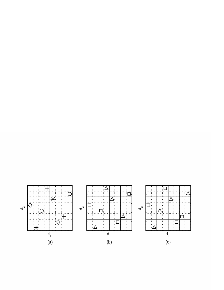
Figure 1: Scatterplots of ${\mbox{\boldmath$d$}}_{1}$ versus ${\mbox{\boldmath$d$}}_{2}$ in Example 1: (a) points represented by $\ast,+,\circ$ and $\lozenge$ correspond to the level combinations (0, 0), (0, 1), (1, 0), and (1, 1) of factors $({\mbox{\boldmath$z$}}_{1},{\mbox{\boldmath$z$}}_{2})$ ; (b) points marked by $\vartriangle$ and $\square$ correspond to the levels 0 and 1 of ${\mbox{\boldmath$z$}}_{1}$; (c) points represented by $\vartriangle$ and $\square$ correspond to the levels 0 and 1 of ${\mbox{\boldmath$z$}}_{2}$.

3 Existence of DCDs

This section focuses on investigating the properties of DCDs and establishing the existence of a DCD$(n,s^{q},p)$, which quantifies all the characteristics of the sub-designs ${\mbox{\boldmath$D$}}_{1}$ and ${\mbox{\boldmath$D$}}_{2}$ in a DCD.

For ease of expression, more notations are introduced. For ${\mbox{\boldmath$D$}}_{1}=({\mbox{\boldmath$z$}}_{1},\dots,{\mbox{\boldmath$z$}}_{q})$ and ${\mbox{\boldmath$D$}}_{2}=({\mbox{\boldmath$d$}}_{1},\dots,{\mbox{\boldmath$d$}}_{p})$ in a DCD, we define $\widetilde{{\mbox{\boldmath$D$}}}_{2}$ and $\widetilde{\widetilde{{\mbox{\boldmath$D$}}}}_{2}$ as,

$$\widetilde{{\mbox{\boldmath$D$}}}_{2}=\left\lfloor\frac{{\mbox{\boldmath$D$}}_{2}}{s}\right\rfloor=(\tilde{{\mbox{\boldmath$d$}}_{1}},\dots,\tilde{{\mbox{\boldmath$d$}}_{p}})~{}\text{and}~{}\widetilde{\widetilde{{\mbox{\boldmath$D$}}}}_{2}=\left\lfloor\frac{\widetilde{{\mbox{\boldmath$D$}}}_{2}}{s}\right\rfloor=(\tilde{\tilde{{\mbox{\boldmath$d$}}_{1}}},\dots,\tilde{\tilde{{\mbox{\boldmath$d$}}_{p}}}),$$ (3.1)

where $\lfloor a\rfloor$ represents the largest integer not exceeding $a$. Since ${\mbox{\boldmath$D$}}_{2}$ is an LH$(n,p)$, we have that $\widetilde{{\mbox{\boldmath$D$}}}_{2}$ is an OA$(n,p,{n}/{s},1)$ and $\widetilde{\widetilde{{\mbox{\boldmath$D$}}}}_{2}$ is an OA$(n,p,{n}/{s^{2}},1)$. Conversely, ${\mbox{\boldmath$D$}}_{2}$ can be obtained from $\widetilde{{\mbox{\boldmath$D$}}}_{2}$ via the level-expansion method.

Theorem 1 provides the necessary and sufficient conditions on both ${\mbox{\boldmath$D$}}_{1}$ and ${\mbox{\boldmath$D$}}_{2}$ to ensure that a DCD exists.

Theorem 1.

Suppose ${\mbox{\boldmath$D$}}_{1}=({\mbox{\boldmath$z$}}_{1},\dots,{\mbox{\boldmath$z$}}_{q})$ is an OA$(n,q,s,2)$, and ${\mbox{\boldmath$D$}}_{2}=({\mbox{\boldmath$d$}}_{1},\dots,{\mbox{\boldmath$d$}}_{p})$ is an LH$(n,p)$. The design ${\mbox{\boldmath$D$}}=({\mbox{\boldmath$D$}}_{1},{\mbox{\boldmath$D$}}_{2})$ is a DCD$(n,s^{q},p)$ if and only if

1. $({\mbox{\boldmath$z$}}_{i},\tilde{{\mbox{\boldmath$d$}}_{k}})$ is an OA$(n,2,s\left({n}/{s}\right),2)$, for any $1\leq i\leq q,1\leq k\leq p$; and

2. $({\mbox{\boldmath$z$}}_{i},{\mbox{\boldmath$z$}}_{j},\tilde{\tilde{{\mbox{\boldmath$d$}}_{k}}})$ is an OA$(n,3,s^{2}\left({n}/{s^{2}}\right),3)$, for any $1\leq i\neq j\leq q,1\leq k\leq p$.

Condition (a) of Theorem 1 is the necessary and sufficient condition for $({\mbox{\boldmath$D$}}_{1},{\mbox{\boldmath$D$}}_{2})$ to be an MCD, see He et al. (2017a). Condition (b) says that for an MCD to be a DCD, $({\mbox{\boldmath$z$}}_{i},{\mbox{\boldmath$z$}}_{j},\tilde{\tilde{{\mbox{\boldmath$d$}}_{k}}})$ must be a full factorial design.

In addition, it is worth noting that Conditions (a) and (b) are independent, that is, if a design satisfies Condition (a), it may not meet Condition (b), vice versa. We give two designs to illustrate this point. Let ${\mbox{\boldmath$D$}}^{(a)}=({\mbox{\boldmath$D$}}_{1},{\mbox{\boldmath$D$}}_{2}^{(a)})$ and ${\mbox{\boldmath$D$}}^{(b)}=({\mbox{\boldmath$D$}}_{1},{\mbox{\boldmath$D$}}_{2}^{(b)})$, where ${\mbox{\boldmath$D$}}_{1}$ is from Table 1, ${\mbox{\boldmath$D$}}_{2}^{(a)}=((1,0,6,7,3,2,4,5)^{T},(0,4,2,6,5,1,7,3)^{T})$ and ${\mbox{\boldmath$D$}}_{2}^{(b)}=\left((6,0,1,4,3,5,7,2)^{T},\right.$ $\left.(2,4,0,5,7,1,6,3)^{T}\right)$. It can be easily seen that ${\mbox{\boldmath$D$}}^{(a)}$ meets Condition (a) but not (b), while ${\mbox{\boldmath$D$}}^{(b)}$ satisfies Condition (b) but not (a).

Remark 1.

In Theorem 1, Condition (a) indicates that $({\mbox{\boldmath$D$}}_{1},\tilde{{\mbox{\boldmath$d$}}_{k}})$ is an OA$(n,q+1,s^{q}\left({n}/{s}\right),2)$. In addition, Condition (b) implies that $({\mbox{\boldmath$D$}}_{1},\tilde{\tilde{{\mbox{\boldmath$d$}}_{k}}})$ is an OA$(n,q+1,s^{q}({n}/{s^{2}}),2)$.

We now revisit Example 1 to show the application of Theorem 1.

Example 2.

(Example 1 continued) For the given ${\mbox{\boldmath$D$}}_{2}$, we can obtain $\widetilde{{\mbox{\boldmath$D$}}}_{2}$ and $\widetilde{\widetilde{{\mbox{\boldmath$D$}}}}_{2}$ via (3.1) and we display these two designs as well as ${\mbox{\boldmath$D$}}_{1}$ in Table 2. It can be checked that $({\mbox{\boldmath$z$}}_{i},\tilde{{\mbox{\boldmath$d$}}_{k}})$ is an OA$(8,2,2\times 4,2)$ and $({\mbox{\boldmath$z$}}_{i},{\mbox{\boldmath$z$}}_{j},\tilde{\tilde{{\mbox{\boldmath$d$}}_{k}}})$ is an OA$(8,3,2,3)$, for any $1\leq i\neq j\leq 2$ and $1\leq k\leq 4$. According to Theorem 1, the design $D$ in Example 1 should be a DCD$(8,2^{2},4)$.

Table 2: The ${\mbox{\boldmath$D$}}_{1}$, $\widetilde{{\mbox{\boldmath$D$}}}_{2}$ and $\widetilde{\widetilde{{\mbox{\boldmath$D$}}}}_{2}$ in Example 2

${\mbox{\boldmath$D$}}_{1}$	$\widetilde{{\mbox{\boldmath$D$}}}_{2}$	$\widetilde{\widetilde{{\mbox{\boldmath$D$}}}}_{2}$
$\begin{array}[]{cc}0&0\\ 1&1\\ 0&1\\ 1&0\\ 0&0\\ 1&1\\ 0&1\\ 1&0\end{array}$	$\begin{array}[]{cccc}0&0&0&0\\ 0&2&2&0\\ 3&1&3&1\\ 3&3&1&1\\ 2&2&2&2\\ 2&0&0&2\\ 1&3&1&3\\ 1&1&3&3\end{array}$	$\begin{array}[]{cccc}0&0&0&0\\ 0&1&1&0\\ 1&0&1&0\\ 1&1&0&0\\ 1&1&1&1\\ 1&0&0&1\\ 0&1&0&1\\ 0&0&1&1\end{array}$

Theorem 1 establishes the existence of DCDs in terms of the relationship between the individual columns in ${\mbox{\boldmath$D$}}_{1}$ and $\tilde{{\mbox{\boldmath$d$}}_{k}}$, and the relationship between any pair of columns in ${\mbox{\boldmath$D$}}_{1}$ and $\tilde{\tilde{{\mbox{\boldmath$d$}}_{k}}}$. Interestingly, we can also give the existence of DCDs in terms of the design property of the entire design ${\mbox{\boldmath$D$}}_{1}$, which shows the required structure of ${\mbox{\boldmath$D$}}_{1}$ in a DCD. The precise result is presented in Theorem 2.

Theorem 2.

A DCD$(n,s^{q},p)$ exists if and only if ${\mbox{\boldmath$D$}}_{1}$ can be partitioned into ${n}/{s^{2}}$ CROA$(s^{2},q,s,2)$’s.

Theorem 2 presents the requirement on ${\mbox{\boldmath$D$}}_{1}$ in a DCD. In the construction of a DCD, the ${\mbox{\boldmath$D$}}_{1}$ required by Theorem 2 is the cornerstone. Since for the given design parameters, only when the expected ${\mbox{\boldmath$D$}}_{1}$ exists we can construct the corresponding ${\mbox{\boldmath$D$}}_{2}$ such that ${\mbox{\boldmath$D$}}=({\mbox{\boldmath$D$}}_{1},{\mbox{\boldmath$D$}}_{2})$ is a DCD.

As an example of Theorem 2, see ${\mbox{\boldmath$D$}}_{1}$ in Table 1. The first four rows and the last four rows of ${\mbox{\boldmath$D$}}_{1}$ are CROA$(4,2,2,2)$’s, respectively. The sufficiency of the proof in fact provides a procedure to construct ${\mbox{\boldmath$D$}}_{2}$’s. The detailed process will be shown in Construction 1 of Section 4.

Theorem 3 below studies the existence of a DCD in terms of the relationship between the columns of ${\mbox{\boldmath$D$}}_{1}$ and the columns of two relevant arrays that we use $B$ and $C$ to denote.

Theorem 3.

Suppose ${\mbox{\boldmath$D$}}_{1}$ is an OA$(n,q,s,2)$ and ${\mbox{\boldmath$D$}}_{2}$ is an LH$(n,p)$. The design ${\mbox{\boldmath$D$}}=({\mbox{\boldmath$D$}}_{1},{\mbox{\boldmath$D$}}_{2})$ is a DCD$(n,s^{q},p)$ if and only if there exist two arrays, ${\mbox{\boldmath$B$}}=OA(n,p,n/s^{2},1)$ and ${\mbox{\boldmath$C$}}=OA(n,p,s,1)$ such that for any $1\leq i\neq j\leq q$ and $1\leq k\leq p$, both $({{\mbox{\boldmath$z$}}}_{i},{{\mbox{\boldmath$z$}}}_{j},{{\mbox{\boldmath$b$}}}_{k})$ and $({{\mbox{\boldmath$z$}}}_{i},{{\mbox{\boldmath$c$}}}_{k},{{\mbox{\boldmath$b$}}}_{k})$ are OA$(n,3,s^{2}\left({n}/{s^{2}}\right),3)$’s, where ${\mbox{\boldmath$z$}}_{i}$ is the $i$th column of ${\mbox{\boldmath$D$}}_{1}$, ${\mbox{\boldmath$b$}}_{k}$ and ${\mbox{\boldmath$c$}}_{k}$ are the $k$th column of $B$ and $C$, respectively, and $\widetilde{{\mbox{\boldmath$D$}}}_{2}$ in (3.1) can be written as $\widetilde{{\mbox{\boldmath$D$}}}_{2}=s{\mbox{\boldmath$B$}}+{\mbox{\boldmath$C$}}$.

Remark 2.

The condition $\widetilde{{\mbox{\boldmath$D$}}}_{2}=s{\mbox{\boldmath$B$}}+{\mbox{\boldmath$C$}}$ in Theorem 3 implies $\widetilde{\widetilde{{\mbox{\boldmath$D$}}}}_{2}={\mbox{\boldmath$B$}}$ which further implies that the space-filling property of ${\mbox{\boldmath$D$}}_{2}$ heavily relies on that of $B$ and is slightly affected by $C$. If $B$ has a better stratification property, so is ${\mbox{\boldmath$D$}}_{2}$. For example, if $B$ is an OA$(n,p,{n}/{s^{2}},2)$ instead of OA$(n,p,{n}/{s^{2}},1)$, ${\mbox{\boldmath$D$}}_{2}$ achieves the stratifications on $({n}/{s^{2}})\times({n}/{s^{2}})$ grids for any two quantitative factors.

Theorems 1, 2 and 3 all provide necessary and sufficient conditions for a DCD to exist. These conditions are essentially the same but described in different ways for different purpose and usages. Theorem 3 reveals that to construct a DCD, we shall find the ${\mbox{\boldmath$D$}}_{1}$, $B$ and $C$ that satisfy the conditions. Next section provides three ways to provide such ${\mbox{\boldmath$D$}}_{1}$, $B$ and $C$.

Before we move to the construction of DCDs in next section, we consider a theoretically and practically important topic in the study of DCDs, that is, the maximum number of $s$-level qualitative factors that an $n$-run DCD can entertain. The following corollary gives the upper bound of the qualitative factors in a DCD.

Corollary 1.

If a DCD with ${\mbox{\boldmath$D$}}_{1}$ being an OA$(n,q,s,2)$ exists, then $q\leqslant s$.

This proof of Corollary 1 is straightforward by Theorem 2 and Lemma 1 of Deng et al. (2015) and thus omitted. This corollary shows that the number of the qualitative factors in a DCD cannot exceed $s$. Although the result seems restrictive, it is still practical. There are applications in the literature that the number of the qualitative factors is no more than the number of the qualitative levels, for example, Phadke (1989) considered a router bit experiment with two qualitative four-level factors and seven quantitative factors. Moreover, when $s$ is a prime power, there always exists a CROA$(s^{2},s,s,2)$ by deleting one column from the saturated OA$(s^{2},s+1,s,2)$. Stacking $n/s^{2}$ such CROAs to obtain a desired ${\mbox{\boldmath$D$}}_{1}$ in Theorem 2, the number of the qualitative factors of the resulting design ${\mbox{\boldmath$D$}}_{1}$ reaches the upper bound, $s$.

4 Construction of DCDs

For constructing DCDs, the computational search approach is often infeasible. This section presents three constructions to generate various DCDs. The two methods in Subsection 4.1 construct DCDs by using the permutation approach, which can entertain a large number of the quantitative factors. Subsection 4.2 can provide DCDs with the guaranteed projection space-filling properties on the quantitative factors, while the number of the quantitative factors in DCDs may be relatively limited. The constructions use orthogonal arrays of strength two or three which are readily available in the textbooks such as Hedayat et al. (1999) and the design catalogues on the websites such as Sloane (2014).

4.1 Constructions of design ${\mbox{\boldmath$D$}}_{2}$ via permutations

In this subsection, we give two procedures based on permutations to construct DCDs with a large number of quantitative factors.

Let ${\mbox{\boldmath$A$}}_{1},\dots,{\mbox{\boldmath$A$}}_{\lambda}$ be OA$(s^{2},q+1,s,2)$’s. Without loss of generality, assume the last column of every ${\mbox{\boldmath$A$}}_{i}$ is $({\bf 0}_{s}^{T},{\bf 1}_{s}^{T},\dots,{\bf(s-1)}_{s}^{T})^{T}$, where ${\mbox{\boldmath$y$}}_{s}$ represents a column vector of length $s$ with all the element being $y$’s. The $\lambda$ OAs will be used to generate ${\mbox{\boldmath$D$}}_{1}$ in this subsection.

One construction procedure of ${\mbox{\boldmath$D$}}_{1}$, $B$ and $C$ in Theorem 3 works as follows and it uses the idea of the proof of Theorem 2.

Construction 1.

• Obtain the array ${\mbox{\boldmath$D$}}_{1}$ by deleting the last column of $({\mbox{\boldmath$A$}}_{1}^{T},\ldots,{\mbox{\boldmath$A$}}_{\lambda}^{T})^{T}$.

• Let ${\mbox{\boldmath$b$}}_{k}={\mbox{\boldmath$v$}}_{k}\otimes{\bf 1}_{s^{2}}$, where ${\mbox{\boldmath$v$}}_{k}$ is a random permutation of $(0,1,\dots,\lambda-1)^{T}$, for $1\leq k\leq p$, and denote ${\mbox{\boldmath$B$}}=({\mbox{\boldmath$b$}}_{1},\dots,{\mbox{\boldmath$b$}}_{p})$.

• Let ${{\mbox{\boldmath$c$}}}_{k}=(({{\mbox{\boldmath$w$}}}_{k1}\otimes{\bf 1}_{s})^{T},\ldots,({{\mbox{\boldmath$w$}}}_{k\lambda}\otimes{\bf 1}_{s})^{T})^{T}$, where ${{\mbox{\boldmath$w$}}}_{kj}$ is a random permutation of $(0,1,\dots,s-1)^{T}$, for $1\leq k\leq p$ and $1\leq j\leq\lambda$, and denote ${\mbox{\boldmath$C$}}=({\mbox{\boldmath$c$}}_{1},\dots,{\mbox{\boldmath$c$}}_{p})$.

• Let $\widetilde{{\mbox{\boldmath$D$}}}_{2}=s{\mbox{\boldmath$B$}}+{\mbox{\boldmath$C$}}$, and obtain ${\mbox{\boldmath$D$}}_{2}=({\mbox{\boldmath$d$}}_{1},\dots,{\mbox{\boldmath$d$}}_{p})$ from $\widetilde{{\mbox{\boldmath$D$}}}_{2}$ via the level-expansion method. Denote ${\mbox{\boldmath$D$}}=({\mbox{\boldmath$D$}}_{1},{\mbox{\boldmath$D$}}_{2})$.

Proposition 1.

The design ${\mbox{\boldmath$D$}}=({\mbox{\boldmath$D$}}_{1},{\mbox{\boldmath$D$}}_{2})$ generated by Construction 1 is a DCD$(\lambda s^{2},s^{q},p)$.

The proof is straightforward, and thus we omit it. In Construction 1, Step 1 is devoted to constructing the ${\mbox{\boldmath$D$}}_{1}$ meets the requirement in Theorem 2. The orthogonal arrays ${\mbox{\boldmath$A$}}_{1},\dots,{\mbox{\boldmath$A$}}_{\lambda}$ are OA$(s^{2},q+1,s,2)$’s. Note that ${\mbox{\boldmath$A$}}_{i}$’s can be either the same or different (isomorphic or non-isomorphic), however, using different ${\mbox{\boldmath$A$}}_{i}$’s is more desirable for generating ${\mbox{\boldmath$D$}}_{1}$ with higher strength. The proposed procedure produces $(s!)^{\lambda s}\cdot(s!)^{\lambda}\cdot\lambda!$ different quantitative columns in Proposition 1, that is, Construction 1 provides the DCDs with a considerable number of quantitative factors. For $2\leq s\leq 11$ and a positive integer $\lambda$, Construction 1 can produce the DCDs with $\lambda s^{2}$ runs, $q$ qualitative factors and $p$ quantitative factors, where $q=s$ for a prime power $s$, $q=2,~{}3$ for $s=6,~{}10$, respectively, and $p\leq(s!)^{\lambda s}\cdot(s!)^{\lambda}\cdot\lambda!$. Details are given in Table 1 of the online supplementary material.

Example 3 illustrates Construction 1. To save the space, we set $p=3$.

Example 3.

Suppose we aim to construct a DCD$(27,3^{3},3)$, that is, $s=3,\lambda=3,q=3,p=3$. We use the three OA$(9,4,3,2)$’s below,

$$\begin{array}[]{ccc}{\mbox{\boldmath$A$}}_{1}=\left[\begin{array}[]{cccc}0&0&0&0\\ 1&1&2&0\\ 2&2&1&0\\ \hdashline 0&2&2&1\\ 1&0&1&1\\ 2&1&0&1\\ \hdashline 0&1&1&2\\ 1&2&0&2\\ 2&0&2&2\end{array}\right],&{\mbox{\boldmath$A$}}_{2}=\left[\begin{array}[]{cccc}0&0&1&0\\ 1&1&0&0\\ 2&2&2&0\\ \hdashline 0&2&0&1\\ 1&0&2&1\\ 2&1&1&1\\ \hdashline 0&1&2&2\\ 1&2&1&2\\ 2&0&0&2\\ \end{array}\right],&{\mbox{\boldmath$A$}}_{3}=\left[\begin{array}[]{cccc}0&0&2&0\\ 1&1&1&0\\ 2&2&0&0\\ \hdashline 0&2&1&1\\ 1&0&0&1\\ 2&1&2&1\\ \hdashline 0&1&0&2\\ 1&2&2&2\\ 2&0&1&2\end{array}\right].\end{array}$$

In Step 1, stack ${\mbox{\boldmath$A$}}_{1},{\mbox{\boldmath$A$}}_{2},{\mbox{\boldmath$A$}}_{3}$ by row and delete the last column of the resulting design to obtain ${\mbox{\boldmath$D$}}_{1}$, which is an OA$(27,3,3,2)$, and can be divided into 3 CROA$(9,3,3,2)$’s. In Steps 2 and 3, let ${\mbox{\boldmath$v$}}_{1}=(1,2,0)^{T},{\mbox{\boldmath$v$}}_{2}=(0,2,1)^{T},{\mbox{\boldmath$v$}}_{3}=(1,0,2)^{T}$, ${\mbox{\boldmath$w$}}_{11}=(0,1,2)^{T}$, ${\mbox{\boldmath$w$}}_{12}=(1,0,2)^{T}$, ${\mbox{\boldmath$w$}}_{13}=(0,2,1)^{T}$, ${\mbox{\boldmath$w$}}_{21}=(1,2,0)^{T}$, ${\mbox{\boldmath$w$}}_{22}=(1,0,2)^{T}$, ${\mbox{\boldmath$w$}}_{23}=(0,1,2)^{T}$, ${\mbox{\boldmath$w$}}_{31}=(2,0,1)^{T}$, ${\mbox{\boldmath$w$}}_{32}=(0,1,2)^{T}$ and ${\mbox{\boldmath$w$}}_{33}=(1,0,2)^{T}$, then by Construction 1, we can obtain

$${\mbox{\boldmath$B$}}=\left(\begin{array}[]{ccccccccccccccccccccccccccc}1&1&1&1&1&1&1&1&1&2&2&2&2&2&2&2&2&2&0&0&0&0&0&0&0&0&0\\ 0&0&0&0&0&0&0&0&0&2&2&2&2&2&2&2&2&2&1&1&1&1&1&1&1&1&1\\ 1&1&1&1&1&1&1&1&1&0&0&0&0&0&0&0&0&0&2&2&2&2&2&2&2&2&2\end{array}\right)^{T}$$

and

$${\mbox{\boldmath$C$}}=\left(\begin{array}[]{ccccccccccccccccccccccccccc}0&0&0&1&1&1&2&2&2&1&1&1&0&0&0&2&2&2&0&0&0&2&2&2&1&1&1\\ 1&1&1&2&2&2&0&0&0&1&1&1&0&0&0&2&2&2&0&0&0&1&1&1&2&2&2\\ 2&2&2&0&0&0&1&1&1&0&0&0&1&1&1&2&2&2&1&1&1&0&0&0&2&2&2\end{array}\right)^{T}.$$

In Step 4, let $\widetilde{{\mbox{\boldmath$D$}}}_{2}=3{\mbox{\boldmath$B$}}+{\mbox{\boldmath$C$}}$ and obtain ${\mbox{\boldmath$D$}}_{2}$. According to Proposition 1, the resulting design ${\mbox{\boldmath$D$}}=({\mbox{\boldmath$D$}}_{1},{\mbox{\boldmath$D$}}_{2})$ is a DCD$(27,3^{3},3)$, listed in Table 3. Moreover, the generated ${\mbox{\boldmath$D$}}_{1}$ is of strength 3. The number of the qualitative factors in this example achieves the upper bound in Corollary 1.

Table 3: ${\mbox{\boldmath$D$}}=({\mbox{\boldmath$D$}}_{1},{\mbox{\boldmath$D$}}_{2})$ in Example 3

${\mbox{\boldmath$D$}}_{1}^{T}$	0	1	2	0	1	2	0	1	2	0	1	2	0	1	2	0	1	2	0	1	2	0	1	2	0	1	2
	0	1	2	2	0	1	1	2	0	0	1	2	2	0	1	1	2	0	0	1	2	2	0	1	1	2	0
	0	2	1	2	1	0	1	0	2	1	0	2	0	2	1	2	1	0	2	1	0	1	0	2	0	2	1
${\mbox{\boldmath$D$}}_{2}^{T}$	9	10	11	13	14	12	15	16	17	22	23	21	19	18	20	24	25	26	2	0	1	7	8	6	4	5	3
	3	5	4	6	7	8	0	1	2	21	22	23	19	20	18	26	24	25	11	10	9	13	14	12	16	15	17
	16	17	15	10	11	9	12	13	14	1	2	0	4	5	3	8	7	6	21	22	23	19	20	18	24	25	26

Remark 3.

If an OA$(\lambda s^{2},q,s,t)$ with $t\geqslant 3$ can be partitioned into $\lambda$ CROA$(s^{2},q,s,2)$’s, a DCD with ${\mbox{\boldmath$D$}}_{1}$ of strength $t\geqslant 3$ can be constructed, such as the ${\mbox{\boldmath$D$}}_{1}$ in Example 3.

We now introduce the second method to construct the required arrays ${\mbox{\boldmath$D$}}_{1}$, $B$ and $C$ in Theorem 3 based on the permutation method.

Construction 2.

• Obtain the array ${\mbox{\boldmath$D$}}_{1}$ by deleting the last column of ${\bf 1}_{\lambda}\otimes{\mbox{\boldmath$A$}}_{1}$.

• Let ${\mbox{\boldmath$B$}}=({\mbox{\boldmath$b$}}_{1},\dots,{\mbox{\boldmath$b$}}_{p})$, where $\{b_{i,k},b_{i+s^{2},k},\dots,b_{i+(\lambda-1)s^{2},k}\}$ is a random permutation of $\{0,1\dots,\lambda-1\}$ and $b_{i,k}$ is the $i$-th entry of ${\mbox{\boldmath$b$}}_{k}$, for $1\leq i\leq s^{2}$ and $1\leq k\leq p$.

• Let ${{\mbox{\boldmath$c$}}}_{k}={\bf 1}_{\lambda}\otimes({\mbox{\boldmath$w$}}_{k}\otimes{\bf 1}_{s})$, where ${{\mbox{\boldmath$w$}}}_{k}$ is a random permutation of $(0,1,\dots,s-1)^{T}$, for $1\leq k\leq p$, and denote ${\mbox{\boldmath$C$}}=({\mbox{\boldmath$c$}}_{1},\dots,{\mbox{\boldmath$c$}}_{p})$.

• Let $\widetilde{{\mbox{\boldmath$D$}}}_{2}=s{\mbox{\boldmath$B$}}+{\mbox{\boldmath$C$}}$, and obtain ${\mbox{\boldmath$D$}}_{2}=({\mbox{\boldmath$d$}}_{1},\dots,{\mbox{\boldmath$d$}}_{p})$ from $\widetilde{{\mbox{\boldmath$D$}}}_{2}$ via the level-expansion method. Denote ${\mbox{\boldmath$D$}}=({\mbox{\boldmath$D$}}_{1},{\mbox{\boldmath$D$}}_{2})$.

Proposition 2.

The design ${\mbox{\boldmath$D$}}=({\mbox{\boldmath$D$}}_{1},{\mbox{\boldmath$D$}}_{2})$ produced by Construction 2 is a DCD$(\lambda s^{2},s^{q},p)$.

In Proposition 2, DCDs with at most $(s!)^{\lambda s}\cdot s!\cdot(\lambda!)^{s^{2}}$ distinct quantitative columns can be generated, which indicates that Construction 2 can also construct the DCDs containing a large number of quantitative factors.

Example 4 below provides an illustration of Construction 2.

Example 4.

Consider generating a DCD$(27,3^{3},3)$ and choose ${\mbox{\boldmath$A$}}_{1}$ shown in Example 3. In Step 1, delete the last column of ${\bf 1}_{\lambda}\otimes{\mbox{\boldmath$A$}}_{1}$ to obtain ${\mbox{\boldmath$D$}}_{1}$. In Step 2, let

$${\mbox{\boldmath$B$}}=\left(\begin{array}[]{ccccccccccccccccccccccccccc}2&0&1&2&0&1&2&0&1&0&1&2&0&1&2&0&1&2&1&2&0&1&2&0&1&2&0\\ 2&1&0&0&2&1&1&0&2&0&2&1&1&0&2&2&1&0&1&0&2&2&1&0&0&2&1\\ 0&2&1&2&1&0&1&0&2&1&0&2&0&2&1&2&1&0&2&1&0&1&0&2&0&2&1\end{array}\right)^{T}.$$

One can easily check that $\{b_{i,k},b_{i+9,k},b_{i+18,k}\}$ is a permutation of $\{0,1,2\}$, for $1\leq i\leq 9$ and $1\leq k\leq 3$. In Step 3, let ${\mbox{\boldmath$w$}}_{1}=(0,1,2)^{T},{\mbox{\boldmath$w$}}_{2}=(1,2,0)^{T}$ and ${\mbox{\boldmath$w$}}_{3}=(2,0,1)^{T}$, and we have

$${\mbox{\boldmath$C$}}=\left(\begin{array}[]{ccccccccccccccccccccccccccc}0&0&0&1&1&1&2&2&2&0&0&0&1&1&1&2&2&2&0&0&0&1&1&1&2&2&2\\ 1&1&1&2&2&2&0&0&0&1&1&1&2&2&2&0&0&0&1&1&1&2&2&2&0&0&0\\ 2&2&2&0&0&0&1&1&1&2&2&2&0&0&0&1&1&1&2&2&2&0&0&0&1&1&1\end{array}\right)^{T}.$$

The obtained design ${\mbox{\boldmath$D$}}=({\mbox{\boldmath$D$}}_{1},{\mbox{\boldmath$D$}}_{2})$ is a DCD, shown in Table 4.

Table 4: ${\mbox{\boldmath$D$}}=({\mbox{\boldmath$D$}}_{1},{\mbox{\boldmath$D$}}_{2})$ in Example 4

${\mbox{\boldmath$D$}}_{1}^{T}$	0	1	2	0	1	2	0	1	2	0	1	2	0	1	2	0	1	2	0	1	2	0	1	2	0	1	2
	0	1	2	2	0	1	1	2	0	0	1	2	2	0	1	1	2	0	0	1	2	2	0	1	1	2	0
	0	2	1	2	1	0	1	0	2	0	2	1	2	1	0	1	0	2	0	2	1	2	1	0	1	0	2
${\mbox{\boldmath$D$}}_{2}^{T}$	19	1	9	22	3	13	25	8	17	0	11	18	5	14	21	6	16	24	10	20	2	12	23	4	15	26	7
	23	12	4	7	26	17	10	1	19	3	22	14	16	8	25	18	9	0	13	5	21	24	15	6	2	20	11
	8	26	17	20	10	2	13	5	21	16	7	25	1	19	11	22	14	3	24	15	6	9	0	18	4	23	12

In practice, for a predetermined $p$, an optimal ${\mbox{\boldmath$D$}}_{2}$ according to some optimization criteria (such as maximin distance, uniform discrepancies, etc) can be found by ranking all possible candidate designs or via the greedy search algorithms such as the simulated annealing or the threshold accepting algorithms if the number of candidate designs is exceedingly large (Morris and Mitchell (1995); Ba et al. (2015)).

4.2 Constructions for the better space-filling property on the quantitative factors

This subsection provides another construction method which uses one array we call $A$ to provide ${\mbox{\boldmath$D$}}_{1}$ and $C$ that is required in Theorem 3. That is, the new construction only involves two arrays $A$ and the $B$. Two specific cases of the construction are provided to produce the required $A$ and $B$, where the resulting DCDs may share some extra high-dimensional space-filling properties among the quantitative factors. Suppose $A$ is an OA$(n,q+1,s,2)$ and $B$ is an OA$(n,p,{n}/{s^{2}},1)$. Construction 3 works as follows.

Construction 3.

• Randomly choose $q$ columns from $A$ to obtain ${\mbox{\boldmath$D$}}_{1}$. Denote the remaining column of $A$ by ${\bf a}^{*}$.

• Let ${\mbox{\boldmath$C$}}=({\mbox{\boldmath$c$}}_{1},\dots,{\mbox{\boldmath$c$}}_{p})$, where ${\mbox{\boldmath$c$}}_{k}$ is obtained by permuting the levels of ${\bf a}^{*}$, for any $1\leq k\leq p$.

• Let $\widetilde{{\mbox{\boldmath$D$}}}_{2}=s{\mbox{\boldmath$B$}}+{\mbox{\boldmath$C$}}$, and obtain ${\mbox{\boldmath$D$}}_{2}=({\mbox{\boldmath$d$}}_{1},\dots,{\mbox{\boldmath$d$}}_{p})$ from $\widetilde{{\mbox{\boldmath$D$}}}_{2}$ via the level-expansion method. Denote ${\mbox{\boldmath$D$}}=({\mbox{\boldmath$D$}}_{1},{\mbox{\boldmath$D$}}_{2})$.

Theorem 4.

Suppose ${{\mbox{\boldmath$A$}}}=({\bf a}_{1},\dots,{\bf a}_{q+1})$ is an OA$(n,q+1,s,2)$ and ${\mbox{\boldmath$B$}}=({\mbox{\boldmath$b$}}_{1},\dots,{\mbox{\boldmath$b$}}_{p})$ is an OA$(n,p,{n}/{s^{2}},1)$. If $({\bf a}_{i},{\bf a}_{j},{\mbox{\boldmath$b$}}_{k})$ is an OA$(n,3,s^{2}\left({n}/{s^{2}}\right),3)$ for any $1\leq i\neq j\leq q+1$ and $1\leq k\leq p$, then the obtained $D$ by Construction 3 above is a DCD$(n,s^{q},p)$.

Theorem 4 tells us that, to construct a DCD$(n,s^{q},p)$, the most important task is to find such two required arrays $A$ and $B$. Under the condition of Theorem 4, it can be verified that the three arrays ${\mbox{\boldmath$D$}}_{1}$, $B$ and $C$ in Construction 3 meet the conditions in Theorem 3. Hence, the obtained $D$ of Construction 3 is a DCD. One can see that Theorem 4 can be regarded as a special case of Theorem 3.

Next, we present an example to illustrate the application of Construction 3.

Example 5.

Suppose that we want to construct a DCD($8,2^{2},4$). Let

$${\mbox{\boldmath$A$}}=({\bf a}_{1},{\bf a}_{2},{\bf a}_{3})=\left(\begin{array}[]{ccc}0&0&0\\ 0&1&1\\ 1&0&1\\ 1&1&0\\ 0&0&0\\ 0&1&1\\ 1&0&1\\ 1&1&0\end{array}\right)\text{and}~{}{\mbox{\boldmath$B$}}=({\mbox{\boldmath$b$}}_{1},{\mbox{\boldmath$b$}}_{2},{\mbox{\boldmath$b$}}_{3},{\mbox{\boldmath$b$}}_{4})=\left(\begin{array}[]{cccc}0&0&0&0\\ 0&1&1&0\\ 1&0&1&0\\ 1&1&0&0\\ 1&1&1&1\\ 1&0&0&1\\ 0&1&0&1\\ 0&0&1&1\end{array}\right).$$

It can be checked that $A$ is an OA$(8,3,2,2)$, $B$ is an OA$(8,4,2,2)$, and $({\bf a}_{i},{\bf a}_{j},{\mbox{\boldmath$b$}}_{k})$ is an OA$(8,3,2,3)$, for $1\leq i\neq j\leq 3,1\leq k\leq 4$. Thus, $A$ and $B$ satisfy the requirements in Theorem 4. In Step 1, select ${\bf a}_{2},{\bf a}_{3}$ of $A$ to be ${\mbox{\boldmath$D$}}_{1}$ and denote ${\bf a}^{*}={\bf a}_{1}$. In Step 2, each column of $C$ is generated by ${\bf a}_{1}$ via the level permutation. Without loss of generality, let ${\mbox{\boldmath$c$}}_{k}={\bf a}_{1}$ for $1\leq k\leq 4$. In Step 3, we can obtain the corresponding $\widetilde{{\mbox{\boldmath$D$}}}_{2}$ and apply the level-expansion method. The resulting design ${\mbox{\boldmath$D$}}=({\mbox{\boldmath$D$}}_{1},{\mbox{\boldmath$D$}}_{2})$ is shown in Example 1. Additionally, $B$ is an orthogonal array of strength 2, therefore, the resulting ${\mbox{\boldmath$D$}}_{2}$ achieves the stratifications on $2\times 2$ grids for any two quantitative factors, which can be verified by Figure 1.

We now present two cases to generate the required arrays $A$ and $B$ in Theorem 4, and they can produce DCDs with $s^{3}$ and $s^{u}$ runs for $u\geqslant 3$, respectively. Besides, Case 1 is suitable for any $s\geqslant 2$, while Case 2 works for any prime power $s$. In both cases, the resulting DCDs enjoy some extra two-dimensional space-filling properties among the quantitative factors.

Case 1.

Let $G$ be an $OA(s^{3},m,s,3)$. Split the columns of $G$ randomly into two arrays, $A$ and $B$, where $A$ has $q+1$ columns and $B$ has $p$ columns, $m=p+q+1$.

The orthogonal array $G$ of strength 3 in Case 1 can be directly taken from the existing websites, such as Sloane (2014).

Proposition 3.

The ${\mbox{\boldmath$D$}}=({\mbox{\boldmath$D$}}_{1},{\mbox{\boldmath$D$}}_{2})$ constructed via Construction 3 by using $A$ and $B$ in Case 1 is a DCD$(s^{3},s^{q},p)$, where $q+p=m-1$. Furthermore, we have

1. ${\mbox{\boldmath$D$}}_{1}$ is an OA$(s^{3},q,s,t)$, where $t=q$, if $q<3$, and $t=3$, if $q\geqslant 3$;

2. $(\tilde{{\mbox{\boldmath$d$}}_{k}},\tilde{{\mbox{\boldmath$d$}}_{k^{\prime}}}),$ for any $1\leq k\neq k^{\prime}\leq p$, achieves the stratification on $s^{2}\times s$ and $s\times s^{2}$ grids; and

3. $\widetilde{\widetilde{{\mbox{\boldmath$D$}}}}_{2}$ is an OA$(s^{3},p,s,t)$, where $t=p$, if $p<3$, and $t=3$, if $p\geqslant 3$.

Parts (b) and (c) in Proposition 3 mean that ${\mbox{\boldmath$D$}}_{2}$ enjoys the two-dimensional and three-dimensional space-filling properties. For $s\leq 10$, the sum of the number of the qualitative and quantitative factors of the DCDs produced by Case 1 of Construction 3 is no more than three for $s=2,3,6,10$, five for $s=4,5$, seven for $s=7$, and nine for $s=8,9$. Table 2 of the online supplementary material shows the details.

We now begin to introduce Case 2, which is based on regular fractional factorial designs (Wu and Hamada (2009)). For any prime power $s$ and any integer $u\geq 3$, let ${\mbox{\boldmath$\xi$}}_{1},\dots,{\mbox{\boldmath$\xi$}}_{u}$ be independent columns of length $s^{u}$ with the entries being from $GF(s)$, the Galois field of order $s$.

Case 2.

• Let

  $$\begin{split}&{\mbox{\boldmath$A$}}=\left\{{\mbox{\boldmath$\xi$}}_{1}+\mu_{2}{\mbox{\boldmath$\xi$}}_{2}~{}|~{}\mu_{2}\in GF(s)\right\}\cup\left\{{\mbox{\boldmath$\xi$}}_{2}\right\}=({\bf a}_{1},\dots,{\bf a}_{s+1}),\\ &{\mbox{\boldmath$R$}}_{v}=\{{\mbox{\boldmath$\xi$}}_{1}+\mu_{2}{\mbox{\boldmath$\xi$}}_{2}+\mu_{v+2}{\mbox{\boldmath$\xi$}}_{v+2}~{}|~{}\mu_{2}\in GF(s),\mu_{v+2}\in GF(s)\backslash\{0\}\}\\ &~{}~{}~{}~{}~{}~{}~{}~{}\cup\{{\mbox{\boldmath$\xi$}}_{2}+\mu_{v+2}{\mbox{\boldmath$\xi$}}_{v+2}~{}|~{}\mu_{v+2}\in GF(s)\backslash\{0\}\}\\ &~{}~{}~{}~{}~{}~{}~{}~{}\cup\{{\mbox{\boldmath$\xi$}}_{v+2}\}=({\mbox{\boldmath$r$}}_{v,1},\dots,{\mbox{\boldmath$r$}}_{v,s^{2}}),\end{split}$$

  where ${\mbox{\boldmath$r$}}_{v,f}$ is a column vector of length $s^{u}$, for $1\leq v\leq u-2$ and $1\leq f\leq s^{2}$.

• For any $1\leq f\leq s^{2},$ let

  $${\mbox{\boldmath$B$}}_{f}=({\mbox{\boldmath$r$}}_{1,f},\dots,{\mbox{\boldmath$r$}}_{u-2,f}){\mbox{\boldmath$T$}},$$

  where

  $${\mbox{\boldmath$T$}}=\left(\begin{array}[]{ccccc}s^{u-3}&1&\cdots&s^{u-5}&s^{u-4}\\ s^{u-4}&s^{u-3}&\cdots&s^{u-6}&s^{u-5}\\ \vdots&\vdots&\vdots&\vdots&\vdots\\ s&s^{2}&\cdots&s^{u-3}&1\\ 1&s&\cdots&s^{u-4}&s^{u-3}\end{array}\right)=({\mbox{\boldmath$t$}}_{1},\dots,{\mbox{\boldmath$t$}}_{u-2}).$$

  There are $u-2$ columns in each ${\mbox{\boldmath$B$}}_{f}.$

• Let ${\mbox{\boldmath$B$}}=({\mbox{\boldmath$B$}}_{1},\dots,{\mbox{\boldmath$B$}}_{s^{2}})=({\mbox{\boldmath$b$}}_{1},\dots,{\mbox{\boldmath$b$}}_{(u-2)s^{2}})$.

Clearly, $A$ consists of the independent columns ${\mbox{\boldmath$\xi$}}_{1},{\mbox{\boldmath$\xi$}}_{2}$ and all possible interactions of these two columns, and thus $A$ has $s+1$ columns. While the column vectors in ${\mbox{\boldmath$R$}}_{v}$ must involve ${\mbox{\boldmath$\xi$}}_{v+2}$ and may contain ${\mbox{\boldmath$\xi$}}_{1}$ and ${\mbox{\boldmath$\xi$}}_{2}$. Lemma 1 summarizes the design properties of ${\mbox{\boldmath$A$}},{\mbox{\boldmath$R$}}_{1},\dots,{\mbox{\boldmath$R$}}_{u-2}$. The proof is straightforward and thus omitted.

Lemma 1.

For ${\mbox{\boldmath$A$}},{\mbox{\boldmath$R$}}_{1},\dots,{\mbox{\boldmath$R$}}_{u-2}$ in Case 2, we have,

1. $A$ is an OA$(s^{u},s+1,s,2)$;

2. $({\mbox{\boldmath$R$}}_{1},\dots,{\mbox{\boldmath$R$}}_{u-2})$ is an OA$(s^{u},(u-2)s^{2},s,2)$;

3. $({\bf a}_{i},{\bf a}_{j},{\mbox{\boldmath$r$}}_{1,f},\dots,{\mbox{\boldmath$r$}}_{u-2,f})$ is an OA$(s^{u},u,s,u)$, for any $1\leq f\leq s^{2}$, $1\leq i\neq j\leq s+1$; and

4. $({\mbox{\boldmath$r$}}_{1,f},\dots,{\mbox{\boldmath$r$}}_{u-2,f},{\mbox{\boldmath$r$}}_{v,l})$ is an OA$(s^{u},u-1,s,u-1)$, for any $1\leq v\leq u-2$, $1\leq f\neq l\leq s^{2}$.

Lemma 1(c) means that taking two distinct columns from $A$, and one column from each ${\mbox{\boldmath$R$}}_{v}$, for $v=1,\ldots,u-2$, the resulting $u$ columns form an $s$-level orthogonal array of $s^{u}$ runs and strength $u$, that is, a full factorial design of $s$ levels and $u$ columns. Similarly, Lemma 1(d) implies that the array of $u-1$ columns, consisting of two distinct columns of ${\mbox{\boldmath$R$}}_{v}$ and one column of each of the remaining $u-3$ arrays ${\mbox{\boldmath$R$}}_{1},\dots,{\mbox{\boldmath$R$}}_{v-1},{\mbox{\boldmath$R$}}_{v+1},\dots,{\mbox{\boldmath$R$}}_{u-2}$, is an orthogonal array of strength $u-1$, i.e., a full factorial design of $s$ levels and $u-1$ columns.

From Lemma 1 and Case 2, we have the following result.

Lemma 2.

For $A$ and $B$ in Case 2, we have

• $({\bf a}_{i},{\bf a}_{j},{\mbox{\boldmath$b$}}_{k})$ is an OA$(s^{u},3,s^{2}(s^{u-2}),3)$, for any $1\leq i\neq j\leq s+1$ and $1\leq k\leq(u-2)s^{2}$; and

• $A$ is an ${\rm OA}(s^{u},s+1,s,2)$ and $B$ is an OA$(s^{u},(u-2)s^{2},s^{u-2},1)$.

Lemma 2 points out that $A$ and $B$ in Case 2 are the required arrays in Theorem 4. For $s=2,u=3$, the two arrays $A$ and $B$ in Case 2 are shown in Example 5.

Proposition 4.

For any prime power $s$ and any integer $u\geqslant 3$, ${\mbox{\boldmath$D$}}=({\mbox{\boldmath$D$}}_{1},{\mbox{\boldmath$D$}}_{2})$ constructed via Construction 3 by using $A$ and $B$ in Case 2 is a DCD$(s^{u},s^{s},(u-2)s^{2})$ with ${\mbox{\boldmath$D$}}_{1}$ being an OA$(s^{u},s,s,2)$ and ${\mbox{\boldmath$D$}}_{2}$ being an LH$(s^{u},(u-2)s^{2})$. In addition, ${\mbox{\boldmath$D$}}_{2}$ has the following properties

1. if $\lfloor(i-1)/(u-2)\rfloor=\lfloor(i^{\prime}-1)/(u-2)\rfloor$, $\tilde{\tilde{{\mbox{\boldmath$d$}}_{i}}}$ and $\tilde{\tilde{{\mbox{\boldmath$d$}}_{i^{\prime}}}}$ achieve $s\times s$ grids stratification; and

2. if $\lfloor(i-1)/(u-2)\rfloor\neq\lfloor(i^{\prime}-1)/(u-2)\rfloor$, $\tilde{\tilde{{\mbox{\boldmath$d$}}_{i}}}$ and $\tilde{\tilde{{\mbox{\boldmath$d$}}_{i^{\prime}}}}$ achieve $s^{u-2}\times s$ and $s\times s^{u-2}$ grids stratification.

Obviously, the number of the qualitative factors for the DCDs in Proposition 4 is $s$, which reaches the upper bound in Corollary 1 and the number of the quantitative factors is $(u-2)s^{2}$.

5 Conclusion

In this paper, we propose $\omega$-way coupled designs with $\omega\geqslant 2$, for computer experiments involving both qualitative and quantitative factors. We focus on the properties and constructions of the two-way coupled designs, namely, doubly coupled designs. Similar to MCDs, such designs are an economical alternative to SLHDs. Different from MCDs, they require that for each level combination of every two qualitative factors, the corresponding design points for quantitative factors form an LHD. This additional requirement leads to the result that given the same run size, DCDs can entertain less qualitative factors than MCDs. In addition, DCDs are equipped with the better stratification properties between the qualitative and quantitative factors than MCDs.

When the design for the qualitative factors ${\mbox{\boldmath$D$}}_{1}$ is an OA$(n,q,s,2)$, the necessary and sufficient conditions for the existence of a DCD are provided and a tight upper bound of the number of the qualitative factors is given. Three construction methods are provided. They are different but related. Particularly, Constructions 1 and 2 are both based on the idea of permutations, but they generate ${\mbox{\boldmath$D$}}_{1},{\mbox{\boldmath$B$}},{\mbox{\boldmath$C$}}$ in different ways. More specifically, Step 1 of Construction 2 uses $\lambda$ identical OAs while ${\mbox{\boldmath$A$}}_{1},\cdots,{\mbox{\boldmath$A$}}_{\lambda}$ used in Step 1 of Construction 1 can be identical, isomorphic or non-isomorphic; Step 2 of Construction 1 is a special case of Step 2 of Construction 2 when $\{b_{i,k},b_{i+s^{2},k},\dots,b_{i+(\lambda-1)s^{2},k}\}$ is the same random permutation of $\{0,1,\cdots,\lambda-1\}$ for $1\leq i\leq s^{2}$; Step 3 of Construction 2 is a special case of Step 3 of Construction 1 when $\omega_{kj}$ is the same permutation of $\{0,1,\cdots,\lambda-1\}$ for $1\leq j\leq\lambda$. Construction 3 is different from Constructions 1 and 2 in that it uses an array $A$ to provide ${\mbox{\boldmath$D$}}_{1}$ and $C$. Thus the building block of Construction 3 is arrays $A$ and $B$ that meet the conditions in Theorem 4. Two cases of such $A$’s and $B$’s are given. Because $B$’s in Case 1 and $R$’s in Case 2 are orthogonal arrays, the ${\mbox{\boldmath$D$}}_{2}$’s of DCDs produced by Construction 3 involving Cases 1 and 2 are orthogonal array-based Latin hypercubes. Constructions 1 and 2 can entertain a large number of the quantitative factors than Construction 3, but their limitation is that the space-filling properties of the designs for the quantitative factors cannot be ensured. On the other hand, the resulting ${\mbox{\boldmath$D$}}_{2}$ constructed by Construction 3 along with Case 1 and Case 2 can guarantee some desirable stratification on grids for the quantitative factors, however, the number of the quantitative factors of the resulting designs may be relatively limited. As all the constructions are algebraic, they do not cost computing time. For the practical use, we list examples of DCDs provided by the proposed construction methods in the online supplementary material.

The needed arrays ${\mbox{\boldmath$D$}}_{1}$, $B$ and $C$ in Theorem 3 can be constructed by other approaches in the future. The methods to generate the two arrays $A$ and $B$ required by Theorem 4 are not limited to the two cases given in this paper, and more pairs of $A$ and $B$ can be considered in the future. Furthermore, we can consider the DCD, ${\mbox{\boldmath$D$}}=({\mbox{\boldmath$D$}}_{1},{\mbox{\boldmath$D$}}_{2})$ with ${\mbox{\boldmath$D$}}_{1}$ being a mixed-level orthogonal array, being an OA of strength $t$, or possessing some good space-filling properties. Study of the space-filling property of ${\mbox{\boldmath$D$}}_{1}$ is an important topic. The work in Zhou and Xu (2014) studied the space-filling property of orthogonal arrays under two commonly used space-filling measures, discrepancy and maximin distance. Because of the requirement relationship between columns in ${\mbox{\boldmath$D$}}_{1}$ and columns in ${\mbox{\boldmath$D$}}_{2}$, it would require additional effort to explore the theoretical space-filling property of ${\mbox{\boldmath$D$}}_{1}$ in a DCD. Another possible direction is to construct DCDs, where ${\mbox{\boldmath$D$}}_{2}$ has the high-dimensional space-filling properties, such as 3 to 4 dimensions. In addition, an interesting but challenging direction is to construct $\omega$-way coupled designs with $\omega>2$. The construction of such designs is not trivial and cannot be easily extended. We hope to study this and report the results in the near future.

Acknowledgements

Partial of the research was done when the first author visited the Department of Mathematics and Statistics at Queen’s University. Yang is supported by the China Scholarship Council, Research start-up funding of Sichuan Normal University and National Natural Science Foundation of China (12101435). Zhou is supported by the National Natural Science Foundation of China (11871288) and Natural Science Foundation of Tianjin (19JCZDJC31100). Lin is supported by the Natural Sciences and Engineering Research Council of Canada. The authors would also like to thank Professor Jianfeng Yang for his valuable suggestions on this topic.

School of Mathematical Sciences & Laurent Mathematics Center, Sichuan Normal University, Chengdu 610066, China E-mail: yangfeng@sicnu.edu.cn

Department of Mathematics and Statistics, Queen’s University, Kingston, ON, K7L 3N6, Canada E-mail: devon.lin@queensu.ca

School of Statistics and Data Science, LPMC & KLMDASR, Nankai University, Tianjin 300071, China E-mail: ydzhou@nankai.edu.cn

School of Statistics, Beijing Normal University, Beijing 100875, China

E-mail: heyuanzhen@bnu.edu.cn

References

- Ba et al. (2015) Ba, S., Myers, W. R and Brenneman, W. A. (2015). Optimal sliced Latin hypercube designs. Technometrics 57, pp. 479-487.
- Chen et al. (2018) Chen, P. H., Santner, T. J., and Dean, A. M. (2018). Sequential pareto minimization of physical systems using calibrated computer simulators. Statistica Sinica 28, pp. 671-692.
- Deng et al. (2015) Deng, X., Hung, Y. and Lin, C. D. (2015). Design for computer experiments with qualitative and quantitative factors. Statistica Sinica 25, pp. 1567-1581.
- Fang et al. (2005) Fang, K. T., Li, R. and Sudjianto, A. (2005). Design and modeling for computer experiments. New York: Chapman and Hall/CRC.
- Georgiou and Efthimiou (2014) Georgiou, S. D. and Efthimiou, I. (2014). Some classes of orthogonal Latin hypercube designs. Statistica Sinica 24, pp. 101-120.
- Han et al. (2009) Han, G., Santner, T. J., Notz, W. I. and Bartel, D. L. (2009). Prediction for computer experiments having quantitative and qualitative input variables. Technometrics 51, pp. 278-288.
- He et al. (2017a) He, Y., Lin, C. D. and Sun, F. (2017a). On the construction of marginally coupled designs. Statistica Sinica 27, pp. 665-683.
- He et al. (2017b) He, Y., Lin, C. D., Sun, F. and Lv, B. J. (2017b). Marginally coupled designs for two-level qualitative factors. Journal of Statistical Planning and Inference 187, pp. 103-108.
- He et al. (2019) He, Y., Lin, C. D. and Sun, F. (2019). Construction of marginally coupled designs by subspace theory. Bernoulli 25, pp. 2163-2182.
- He and Tang (2013) He, Y. and Tang, B. (2013). Strong orthogonal arrays and associated Latin hypercubes for computer experiments. Biometrika 100, pp. 254-260.
- Hedayat et al. (1999) Hedayat, A. S., Sloane, N. J. A., Stufken, J. (1999). Orthogonal Arrays: Theory and Application. Springer, New York.
- Huang et al. (2016) Huang, H., Lin, D. K. J., Liu, M. Q. and Yang, J. (2016). Computer experiments with both qualitative and quantitative variables. Technometrics 58, pp. 495-507.
- Huang et al. (2021) Huang, H., Yu, H., Liu, M. Q. and Wu, D. (2021). Construction of uniform designs and complex-structured uniform designs via partitionable t-designs Statistica Sinica 31, pp. 1689-1706.
- Hung et al. (2009) Hung, Y., Joseph, V. R. and Melkote, S. N. (2009). Design and analysis of computer experiments with branching and nested factors. Technometrics 51, pp. 354-365.
- Joseph et al. (2007) Joseph, V. R. and Delaney, J. D. (2007). Functionally induced priors for the analysis of experiments. Technometrics 49, pp. 1-11.
- Joseph and Hung (2008) Joseph, V.R. and Hung, Y. (2008). Orthogonal-maximin Latin hypercube designs. Statistica Sinica 18, pp. 171-186.
- Li et al. (2020) Li, W., Liu, M. Q and Tang, B. (2020). A method of constructing maximin distance designs. Biometrika. doi: 10.1093/biomet/asaa089.
- Long and Bartel (2006) Long, J. P. and Bartel, D. L. (2006). Surgical variables affect the mechanics of a hip resurfacing system. Clinical Orthopaedics and Related Research 453, pp. 115-122.
- McKay et al. (1979) McKay, M. D. Beckman, R. J. and Conover, W. J. (1979). A comparison of three methods for selecting values of input variables in the analysis of output from a computer code. Technometrics 21, pp. 239-245.
- Morris and Mitchell (1995) Morris, M. D. and Mitchell, T. J. (1995). Exploratory designs for computational experiments. Journal of Statistical Planning and Inference 43, pp. 381-402.
- Owen (1992) Owen, A. B. (1992). Orthogonal arrays for computer experiments, integration and visuazation. Statistica Sinica 2, pp. 439-452.
- Phadke (1989) Phadke, M. S. (1989). Quality engineering using robust design. Englewood Cliffs, NJ: Prentice-Hall.
- Qian (2012) Qian, P. Z. G. (2012). Sliced Latin hypercube designs. Journal of the American Statistical Association 107, pp. 393-399.
- Qian et al. (2008) Qian, P. Z. G., Wu, H. and Wu, C. F. J. (2008). Gaussian process models for computer experiments with qualitative and quantitative factors. Technometrics 50, pp. 383-396.
- Rawlinson et al. (2006) Rawlinson, J. J., Furman, B. D., Li, S., Wright, T. M. and Bartel, D. L. (2006). Retrieval, experimental, and computational assessment of the performance of total knee replacements. Journal of Orthopaedic Research Official Publication of the Orthopaedic Research Society 24, pp. 1384-1394.
- Santner et al. (2003) Santner, T. J., Williams, B. J. and Notz, W. I. (2003). The design and analysis of computer experiments. New York: Springer.
- Shi and Tang (2020) Shi, C. and Tang, B. (2020). Construction results for strong orthogonal arrays of strength three. Bernoulli 26, pp. 418-431.
- Sloane (2014) Sloane, N. J. A. (2014). http://neilsloane.com/oadir/.
- Sun and Tang (2017) Sun, F. and Tang, B. (2017). A general rotation method for orthogonal Latin hypercubes. Biometrika 104, pp. 465-472.
- Tang (1993) Tang, B. (1993). Orthogonal array-based Latin hypercubes. Journal of the American Statistical Association 88, pp. 1392-1397.
- Wang et al. (2018) Wang, L., Xiao, Q. and Xu, H. (2018). Optimal maximin -distance Latin hypercube designs based on good lattice point designs. The Annals of Statistics 46, pp. 3741šC66.
- Wang et al. (2018) Wang, L., Sun, F., Lin, D. K. J., and Liu, M. Q. (2018). Construction of orthogonal symmetric Latin hypercube designs. Statistica Sinica 28, pp. 1503-1520.
- Wang et al. (2021) Wang, C., Yang, J. and Liu, M. Q. (2021). Construction of strong group-orthogonal arrays. Statistica Sinica, online, doi:10.5705/ss.202020.0110.
- Wu and Hamada (2009) Wu, C. F. J. and Hamada, M. (2009). Experiments: planning, analysis, and optimization. New Jersey: John Wiley & Sons, Inc.
- Xiao and Xu (2018) Xiao, Q. and Xu, H. (2018). Construction of maximin distance designs via level permutation and expansion. Statistica Sinica 28(3), pp. 1395-1414.
- Zhou et al. (2021) Zhou, W., Yang, J. and Liu, M. Q. (2021). Construction of orthogonal marginally coupled designs. Statistical Papers 62, pp., 1795-1820.
- Zhou et al. (2011) Zhou, Q., Qian, P. Z. G. and Zhou, S. (2011). A simple approach to emulation for computer models with qualitative and quantitative factors. Technometrics 53, pp. 266-273.
- Zhou and Tang (2019) Zhou, Y. and Tang, B. (2019). Column-Orthogonal Strong Orthogonal Arrays of Strength Two Plus and Three Minus. Biometrika 106, pp. 997-1004.
- Zhou and Xu (2014) Zhou, Y. D. and Xu, H. (2014). Space-filling fractional factorial designs. Journal of the American Statistical Association 109(507), pp. 1134-1144.