The $Z_{3}$ soft breaking in the I(2+1)HDM
and its probes at present and future colliders

Abstract

A $Z_{3}$ symmetric 3-Higgs Doublet Model (3HDM) with two inert doublets and one active doublet (that plays the role of the Higgs doublet), the so-called I(2+1)HDM, is studied. We discuss the behaviour of this 3HDM realisation when one allows for a $Z_{3}$ soft breaking term. Such a symmetry enables the presence of a two-component Dark Matter (DM) scenario in the form of “Hermaphrodite DM”, where the two inert candidates have opposite CP parity and are protected by this discrete symmetry from decaying into Standard Model (SM) particles. Furthermore, the two DM states are potentially distinguishable from each other as they cannot be subsumed into a complex field, having different masses and gauge couplings. With this in mind, we study differential spectra with a distinctive shape from which the existence of two different DM component distributions could be easily inferred. We prove this to be possible at the Large Hadron Collider (LHC) via the $q\bar{q}\to 2l+H_{1}H_{1}$ and $q\bar{q}\to 2l+A_{1}A_{1}$ processes as well as at a future electron-positron machine via the $e^{+}e^{-}\to 2l+H_{1}H_{1}$ and $e^{+}e^{-}\to 2l+A_{1}A_{1}$ channels, where $l=e,\mu$.

I Introduction

A Higgs boson was discovered at the Large Hadron Collider (LHC) in July 2012 [1, 2] and it has been shown that its nature is consistent with the one of the Standard Model (SM), which contains only one SU(2) doublet field. However, no compelling principle has ever been put forward that constrains the Higgs sector responsible for Electro-Weak Symmetry Breaking (EWSB) and mass generation to be the one of the SM. In particular, there is no reason which forbids introducing new fields into the (pseudo)scalar sector of the underlying theory.

There are many possibilities to extend the Higgs sector of the SM. As Nature seems to prefer doublet (pseudo)scalar fields, one could well restrict oneself to extensions of the SM that only include such representations. Indeed, the ensuing $N$-Higgs Doublet Model (NHDM) is a simple and attractive example, where the Higgs sector contains $N$ such fields. The extension with doublet (pseudo)scalar fields also keeps $\rho=1$ at the tree level. However, NHDMs generally lead to dangerous Flavour Changing Neutral Currents (FCNCs). In order to suppress these, a discrete symmetry is often utilised. For example, in the 2HDM, which is well studied in the literature, a softly broken $Z_{2}$ symmetry is usually introduced. Under this $Z_{2}$ symmetry, one doublet is odd, and the other doublet is even. Depending on the $Z_{2}$ parity assignment for the SM fermions, 2HDMs are then classified into four types [3, 4, 5].

There are reasons to consider this kind of SM extension, as there are some problems that the SM cannot explain, calling for new physics. For example, within the SM, there is no viable candidate for Dark Matter (DM), there is no successful mechanism for baryogenesis, there is no dynamics that explains the smallness of the neutrino masses and so on. One should then expect that Beyond the SM (BSM) scenarios can solve these problems, and specifying the Higgs sector provides a vital clue to explore such new physics. NHDMs can, in particular, afford one with viable DM candidates.

For example, the so-called inert 2HDM, also acronym IDM, provides one such DM candidate. In this model, even parity is assigned to the SM fermions, there is no softly broken term acting on the $Z_{2}$ symmetry in the Higgs potential, and only the $Z_{2}$ even doublet gets a Vacuum Expectation Value (VEV) [6]. Since the $Z_{2}$ is kept unbroken, the lightest $Z_{2}$ odd scalar is, therefore, stable, and it can be a DM if the particle is neutral.

The inert sector of an NHDM with more than two doublets also provides DM candidates. In the case of a 3-Higgs Doublet Model (3HDM), there are many possibilities to impose a discrete symmetry and trigger its breaking patterns. DM properties in an unbroken $Z_{3}$ symmetry model that lead to two inert doublets are discussed in Ref. [7]. If the CP symmetry is unbroken in the inert sector, the lightest $Z_{3}$ charged particles in the CP-odd and CP-even sectors are individually stable. Thus two DM candidates with opposite CP charges are provided. This realisation is called a “Hermaphrodite DM” scenario.

In this paper, we analyse collider signals of this scenario. Since the two DM particles interact with the $Z$ and $W$ gauge bosons and the SM Higgs boson, they are produced at collider experiments such as the LHC and/or a future $e^{+}e^{-}$ collider. We will prove that it should be possible to reveal both these two DM candidates by isolating phenomenological properties of processes leading to the same final state, proceeding through the two different states and pointing to their simultaneous presence.

This paper is organised as follows. Sec. II introduces the model with its Hermaphrodite DM scenario. In Sec. III, we discuss the parameters used in our analysis. We show our numerical results in Sec. IV. Finally, we give our conclusions in Sec. V.

II The model

II.1 Lagrangian

In this paper, we consider an extended Higgs sector with three Higgs doublets $\phi_{i}~{}(i=1,2,3)$. We impose a $Z_{3}$ symmetry under which the three doublets transform as

$$\phi_{1}\to\omega\phi_{1}\;,\quad\phi_{2}\to\omega^{2}\phi_{2}\;,\quad\phi_{3}\to\phi_{3}\;,$$ (1)

with $\omega$ being a complex cubic root of unity, i.e., $\omega=e^{2\pi i/3}$. The symmetric Higgs potential is given by

$$V=V_{0}+V_{Z_{3}}$$ (2)

where $V_{0}$ is an invariant part under any phase rotation given by

$$V_{0}= -\mu^{2}_{1}(\phi_{1}^{\dagger}\phi_{1})-\mu^{2}_{2}(\phi_{2}^{\dagger}\phi_{2})-\mu^{2}_{3}(\phi_{3}^{\dagger}\phi_{3})$$ (3)

$$+\lambda_{11}(\phi_{1}^{\dagger}\phi_{1})^{2}+\lambda_{22}(\phi_{2}^{\dagger}\phi_{2})^{2}+\lambda_{33}(\phi_{3}^{\dagger}\phi_{3})^{2}$$

$$+\lambda_{12}(\phi_{1}^{\dagger}\phi_{1})(\phi_{2}^{\dagger}\phi_{2})+\lambda_{23}(\phi_{2}^{\dagger}\phi_{2})(\phi_{3}^{\dagger}\phi_{3})+\lambda_{31}(\phi_{3}^{\dagger}\phi_{3})(\phi_{1}^{\dagger}\phi_{1})$$

$$+\lambda^{\prime}_{12}(\phi_{1}^{\dagger}\phi_{2})(\phi_{2}^{\dagger}\phi_{1})+\lambda^{\prime}_{23}(\phi_{2}^{\dagger}\phi_{3})(\phi_{3}^{\dagger}\phi_{2})+\lambda^{\prime}_{31}(\phi_{3}^{\dagger}\phi_{1})(\phi_{1}^{\dagger}\phi_{3})$$

and $V_{Z_{3}}$ is a collection of extra terms ensuring the $Z_{3}$ symmetry given by

$$V_{Z_{3}}=\lambda_{1}(\phi_{2}^{\dagger}\phi_{1})(\phi_{3}^{\dagger}\phi_{1})+\lambda_{2}(\phi_{1}^{\dagger}\phi_{2})(\phi_{3}^{\dagger}\phi_{2})+\lambda_{3}(\phi_{1}^{\dagger}\phi_{3})(\phi_{2}^{\dagger}\phi_{3})+\text{h.c.}$$ (4)

We adopt an ansatz that only $\phi_{3}$ has a VEV. With this assumption, the EW symmetry is broken by $\langle\phi_{3}\rangle$ while the $Z_{3}$ symmetry is (initially) unbroken. A physical component in the $Z_{3}$ singlet field $\phi_{3}$ behaves like the SM Higgs boson, so we describe it as such using the label $h$. Also, all SM particles have a $Z_{3}$ zero charge, so that only $\phi_{3}$ will couple to fermions. The Yukawa Lagrangian is given by

$$\mathcal{L}_{Y} = \Gamma^{u}_{mn}\bar{q}_{m,L}\tilde{\phi}_{3}u_{n,R}+\Gamma^{d}_{mn}\bar{q}_{m,L}\phi_{3}d_{n,R}$$ (5)

$$+\Gamma^{e}_{mn}\bar{l}_{m,L}\phi_{3}e_{n,R}+\Gamma^{\nu}_{mn}\bar{l}_{m,L}\tilde{\phi}_{3}{\nu}_{n,R}+\text{h.c.}$$

Thanks to the $Z_{3}$ symmetry, the lightest components of $\phi_{1}$ and $\phi_{2}$ can be stable, and they both are DM candidates. Given that $\phi_{1}$ and $\phi_{2}$ are inert, this model is termed I(2+1)HDM [8, 9]. Since the CP symmetry is also kept in the potential, the combination of the CP and $Z_{3}$ symmetries predicts that these two DM candidates are such that one is CP-even and the other is CP-odd. However, evidently not being the real and imaginary part of a complex field (as it will be clear below), such a two-component DM is aptly named Hermaphrodite DM [9].

As we will discuss later, the model with the softly broken term, only affecting the inert sector,

$$V_{\not{Z_{3}}}=-\mu_{12}^{2}(\phi_{1}^{\dagger}\phi_{2})+\text{h.c.}$$ (6)

is the one interesting from the phenomenological point of view, though. In fact, to realise proper EWSB, the parameter $\mu_{12}^{2}$ must be small, thus allowing for a $Z_{3}$ symmetry soft breaking. As a consequence, the stability of the DM candidates is not affected.

II.2 The physical eigenstates

The scalar potential acquires a minimum at the point

$$\phi_{1}=\left(\begin{array}[]{c}{\scriptstyle{H^{0+}_{1}}}\\ \frac{H^{0}_{1}+iA^{0}_{1}}{\sqrt{2}}\end{array}\right),\qquad\phi_{2}=\left(\begin{array}[]{c}{\scriptstyle{H^{0+}_{2}}}\\ \frac{H^{0}_{2}+iA^{0}_{2}}{\sqrt{2}}\end{array}\right),\qquad\phi_{3}=\left(\begin{array}[]{c}{\scriptstyle{H^{0+}_{3}}}\\ \frac{H_{3}^{0}+v+iA^{0}_{3}}{\sqrt{2}}\end{array}\right),$$ (7)

where $v^{2}=\mu_{3}^{2}/\lambda_{33}$. Expanding the potential around the vacuum point we obtain the mass spectrum. In the model that allows a soft breaking of the $Z_{3}$ symmetry we have the following.

• The neutral sector, CP-even scalars:

  $$\textbf{h}=H_{3}^{0}:\quad m^{2}_{h}=2\mu_{3}^{2}=2\lambda_{33}v^{2}.$$ (8)

  $$\textbf{H}_{1}=\cos\theta_{h}H^{0}_{1}+\sin\theta_{h}H^{0}_{2}$$

  $$\hskip 28.45274ptm^{2}_{H_{1}}=(-\mu^{2}_{1}+\Lambda_{1})\cos^{2}\theta_{h}+(-\mu^{2}_{2}+\Lambda_{2})\sin^{2}\theta_{h}-(2\mu^{2}_{12}-\lambda_{3}v^{2})\sin\theta_{h}\cos\theta_{h}.$$

  $$\textbf{H}_{2}=-\sin\theta_{h}H^{0}_{1}+\cos\theta_{h}H^{0}_{2}$$

  $$\hskip 28.45274ptm^{2}_{H_{2}}=(-\mu^{2}_{1}+\Lambda_{1})\sin^{2}\theta_{h}+(-\mu^{2}_{2}+\Lambda_{2})\cos^{2}\theta_{h}+(2\mu^{2}_{12}-\lambda_{3}v^{2})\sin\theta_{h}\cos\theta_{h}.$$

• The neutral sector, CP-odd scalars:

  $$\textbf{A}_{1}=\cos\theta_{a}A^{0}_{1}+\sin\theta_{a}A^{0}_{2}$$ (9)

  $$\hskip 28.45274ptm^{2}_{A_{1}}=(-\mu^{2}_{1}+\Lambda_{1})\cos^{2}\theta_{a}+(-\mu^{2}_{2}+\Lambda_{2})\sin^{2}\theta_{a}-(2\mu^{2}_{12}+\lambda_{3}v^{2})\sin\theta_{a}\cos\theta_{a}.$$

  $$\textbf{A}_{2}=-\sin\theta_{a}A^{0}_{1}+\cos\theta_{a}A^{0}_{2}$$

  $$\hskip 28.45274ptm^{2}_{A_{2}}=(-\mu^{2}_{1}+\Lambda_{1})\sin^{2}\theta_{a}+(-\mu^{2}_{2}+\Lambda_{2})\cos^{2}\theta_{a}+(2\mu^{2}_{12}+\lambda_{3}v^{2})\sin\theta_{a}\cos\theta_{a}.$$

• The charged sector:

  $$\textbf{H}^{\pm}_{1}=\cos\theta_{c}H^{0\pm}_{1}+\sin\theta_{c}H^{0\pm}_{2}$$ (10)

  $$\hskip 28.45274ptm^{2}_{H^{\pm}_{1}}=(-\mu^{2}_{1}+\frac{1}{2}\lambda_{31}v^{2})\cos^{2}\theta_{c}+(-\mu^{2}_{2}+\frac{1}{2}\lambda_{23}v^{2})\sin^{2}\theta_{c}-2\mu^{2}_{12}\sin\theta_{c}\cos\theta_{c}.$$

  $$\textbf{H}^{\pm}_{2}=-\sin\theta_{c}H^{0\pm}_{1}+\cos\theta_{c}H^{0\pm}_{2}$$

  $$\hskip 28.45274ptm^{2}_{H^{\pm}_{2}}=(-\mu^{2}_{1}+\frac{1}{2}\lambda_{31}v^{2})\sin^{2}\theta_{c}+(-\mu^{2}_{2}+\frac{1}{2}\lambda_{23}v^{2})\cos^{2}\theta_{c}+2\mu^{2}_{12}\sin\theta_{c}\cos\theta_{c}.$$

Here, $\Lambda_{1}=(\lambda_{31}+\lambda^{\prime}_{31})v^{2}/2$ and $\Lambda_{1}=(\lambda_{23}+\lambda^{\prime}_{23})v^{2}/2$. The angles $\theta_{h},\theta_{a},\theta_{c}$ are the mixing angles for the scalar, pseudoscalar an charged mass-squared matrices, respectively, such that:

$$\tan 2\theta_{c}=\frac{4\mu_{12}^{2}}{2\mu_{1}^{2}-\lambda_{31}v^{2}-2\mu_{2}^{2}+\lambda_{23}v^{2}}=\varepsilon_{c},$$

$$\tan 2\theta_{h}=\frac{-\lambda_{3}v^{2}+2\mu_{12}^{2}}{\mu_{1}^{2}-\Lambda_{1}-\mu_{2}^{2}+\Lambda_{2}}=-\frac{\lambda_{3}v^{2}}{\mu^{2}_{1}-\Lambda_{1}-\mu^{2}_{2}+\Lambda_{2}}+\varepsilon_{h},$$

$$\tan 2\theta_{a}=\frac{\lambda_{3}v^{2}+2\mu_{12}^{2}}{\mu_{1}^{2}-\Lambda_{1}-\mu_{2}^{2}+\Lambda_{2}}=\frac{\lambda_{3}v^{2}}{\mu^{2}_{1}-\Lambda_{1}-\mu^{2}_{2}+\Lambda_{2}}+\varepsilon_{h},$$ (11)

in terms of the small parameter $\varepsilon_{h}=\frac{2\mu_{12}^{2}}{\mu^{2}_{1}-\Lambda_{1}-\mu^{2}_{2}+\Lambda_{2}}$. From the expressions above we can extract the relation $\tan 2\theta_{a}=-\tan 2\theta_{h}+2\varepsilon_{h}$. Since the $Z_{3}$ is softly broken via the small $\mu_{12}^{2}$ term, then we can write the rotation angles as

$$\theta_{a}=-\theta_{h}+\epsilon_{h}\quad\text{and}\quad\theta_{c}=\epsilon_{c}.$$ (12)

The masses squared for the (pseudo)scalars are

$$m_{H_{1}}^{2} = (-\mu_{1}^{2}+\Lambda_{1})\cos^{2}\theta_{h}+(-\mu_{2}^{2}+\Lambda_{2})\sin^{2}\theta_{h}-\frac{1}{2}(2\mu_{12}^{2}-\lambda_{3}v^{2})\sin 2\theta_{h},$$ (13)

$$m_{A_{1}}^{2} = m_{H_{1}}^{2}+\left[2\mu_{12}^{2}+\epsilon_{h}(-\mu_{1}^{2}+\Lambda_{1}+\mu_{2}^{2}-\Lambda_{2})\right]\sin 2\theta_{h}-\epsilon_{h}(2\mu_{12}^{2}+\lambda_{3}v^{2})\cos 2\theta_{h},$$

$$m_{H_{2}}^{2} = (-\mu_{1}^{2}+\Lambda_{1})\sin^{2}\theta_{h}+(-\mu_{2}^{2}+\Lambda_{2})\cos^{2}\theta_{h}+\frac{1}{2}(2\mu_{12}^{2}-\lambda_{3}v^{2})\sin 2\theta_{h},$$

$$m_{A_{2}}^{2} = m_{H_{2}}^{2}-\left[2\mu_{12}^{2}+\epsilon_{h}(-\mu_{1}^{2}+\Lambda_{1}+\mu_{2}^{2}-\Lambda_{2})\right]+\epsilon_{h}(2\mu_{12}^{2}+\lambda_{3}v^{2})\cos 2\theta_{h}.$$

As we have mentioned above, the CP symmetry makes $H_{1}$ and $A_{1}$ stable, so they can both be DM. After EWSB, we have the vertex $H_{1}A_{1}Z\propto\cos 2\theta_{h}+\epsilon_{h}\sin 2\theta_{h}$, which leads to a too large cross-section for DM scattering off nuclei and thus direct detection immediately excludes the scenario. In order to avoid it, the coupling constant of this vertex should be significantly suppressed. When we choose $\theta_{h}=\pi/4$, the vertex is proportional to $\epsilon_{h}$, and it is thus expected to be small. Note that $\epsilon_{h}=0$ is satisfied in the $Z_{3}$ symmetric limit and two DM candidates, $H_{1}$ and $A_{1}$ are degenerate in mass, $m_{H_{1}}=m_{A_{1}}$.

III Parameters for the analysis

The input parameters

As mentioned, in order to avoid the model being ruled out by direct detection bounds, we will consider the limit $\theta_{h}=\pi/4$ where the masses squared can be written as follows:

$$m_{H_{1}}^{2} = \frac{1}{2}(-\mu_{1}^{2}+\Lambda_{1})+\frac{1}{2}(-\mu_{2}^{2}+\Lambda_{2})-\frac{1}{2}(2\mu_{12}^{2}-\lambda_{3}v^{2}),$$

$$m_{A_{1}}^{2} = m_{H_{1}}^{2}+\left[2\mu_{12}^{2}+\epsilon_{h}(-\mu_{1}^{2}+\Lambda_{1}+\mu_{2}^{2}-\Lambda_{2})\right]$$ (14)

$$m_{H_{2}}^{2} = \frac{1}{2}(-\mu_{1}^{2}+\Lambda_{1})+\frac{1}{2}(-\mu_{2}^{2}+\Lambda_{2})+\frac{1}{2}(2\mu_{12}^{2}-\lambda_{3}v^{2}),$$

$$m_{A_{2}}^{2} = m_{H_{2}}^{2}-\left[2\mu_{12}^{2}+\epsilon_{h}(-\mu_{1}^{2}+\Lambda_{1}+\mu_{2}^{2}-\Lambda_{2})\right],$$ (15)

$$m_{H_{1}^{\pm}}^{2} = -\mu_{1}^{2}+\frac{v^{2}}{2}\lambda_{31}-2\mu_{12}^{2}\epsilon_{c},$$

$$m_{H_{2}^{\pm}}^{2} = -\mu_{2}^{2}+\frac{v^{2}}{2}\lambda_{23}+2\mu_{12}^{2}\epsilon_{c}.$$ (16)

The input parameters $\lambda_{23},\lambda_{13},\lambda_{23}^{\prime},\lambda_{31}^{\prime},\mu_{1}^{2}$ and $\mu_{2}^{2}$ can be rewritten in terms of the physical observables $m_{H_{1}},m_{H_{2}},m_{H_{1}}^{\pm},m_{H_{2}}^{\pm},\lambda_{1}$ and $\lambda_{2}$. Introducing

$$\Delta_{h}=m_{A_{1}}-m_{H_{1}}$$ (17)

$$\Delta_{c}=m_{H_{1}^{\pm}}-m_{H_{1}},$$ (18)

$$\delta_{c}=m_{H_{2}^{\pm}}-m_{H_{1}^{\pm}},$$ (19)

$$\Delta_{n}=m_{A_{2}}-m_{H_{1}}>50~{}{\rm GeV},$$ (20)

$$\Delta_{n}^{\prime}=m_{H_{2}}-m_{A_{1}},$$ (21)

$$m_{H_{2}}^{2}\approx m_{A_{2}}^{2}+2\mu_{12}^{2},$$ (22)

$$g_{1} = \frac{g_{hH_{1}H_{1}}}{v}=\frac{1}{2}(\lambda_{23}+2\lambda_{3}+\lambda_{31}+\lambda_{23}^{\prime}+\lambda_{31}^{\prime}),$$

$$g_{2} = \frac{g_{hH_{1}H_{2}}}{v}=\frac{1}{2}(\lambda_{23}-\lambda_{31}+\lambda_{23}^{\prime}-\lambda_{31}^{\prime}),$$ (23)

where $g_{hH_{1}H_{1}}$ and $g_{hH_{1}H_{2}}$ are the coefficients of the vertices $hH_{1}H_{1}$ and $hH_{1}H_{2}$, respectively, for $\epsilon_{h}\sim 0$, the Lagrangian parameters in terms of the observables reduce to:

$$\lambda_{23} = \frac{1}{v^{2}}\left((g1+g2)v^{2}-2m_{H_{1}}^{2}+2m_{H_{2}^{\pm}}\right)-\frac{2\mu_{12}^{2}}{v^{2}},$$ (24)

$$\lambda_{31} = \frac{1}{v^{2}}\left((g1-g2)v^{2}-2m_{H_{1}}^{2}+2m_{H_{1}^{\pm}}\right)+\frac{2\mu_{12}^{2}}{v^{2}},$$

$$\lambda_{23}^{\prime} = \frac{1}{v^{2}}\left(m_{H_{1}}^{2}+m_{H_{2}}^{2}-2m_{H_{2}^{\pm}}^{2}\right),$$

$$\lambda_{31}^{\prime} = \frac{1}{v^{2}}\left(m_{H_{1}}^{2}+m_{H_{2}}^{2}-2m_{H_{1}^{\pm}}^{2}\right),$$

$$\lambda_{3} = \frac{1}{v^{2}}\left(m_{H_{1}}^{2}-m_{H_{2}}^{2}+2\mu_{12}^{2}\right),$$

$$\mu_{1}^{2} = \frac{1}{2}\left((g_{1}-g_{2})v^{2}-2m_{H_{1}}^{2}\right)+\frac{2\mu_{12}^{2}}{v^{2}},$$

$$\mu_{2}^{2} = \frac{1}{2}\left((g_{1}+g_{2})v^{2}-2m_{H_{1}}^{2}\right)-\frac{2\mu_{12}^{2}}{v^{2}}.$$

Constraints on the model parameters

All the Benchmark Points (BPs) considered in this study agree with the latest theoretical and experimental constraints that are applicable to the model, which are described in detail in [10, 9]. For convenience, we recap these here. As $\phi_{3}$ is identified with the SM Higgs doublet, $\mu_{3}$ and $\lambda_{33}$ are Higgs field parameters and can be written in terms of the mass of the Higgs boson. We use the value $m_{h}=125$ GeV for the latter, so that

$$m^{2}_{h}=2\mu^{2}_{3}=2\lambda_{33}v^{2}.$$ (25)

In agreement with perturbativity bounds and unitary conditions, we take the absolute values $|\lambda_{i}|\leq 3\pi$. For the potential to be bounded from below, the following conditions are required

$$\bullet~{}\lambda_{11},\,\lambda_{22},\,\lambda_{33}\geq 0,$$ (26)

$$\bullet~{}\lambda_{12}+\lambda^{\prime}_{12}+\sqrt{\lambda_{11}\lambda_{22}}\geq 0,$$

$$\bullet~{}\lambda_{23}+\lambda^{\prime}_{23}+\sqrt{\lambda_{22}\lambda_{33}}\geq 0,$$

$$\bullet~{}\lambda_{31}+\lambda^{\prime}_{31}+\sqrt{\lambda_{33}\lambda_{11}}\geq 0,$$

$$\bullet~{}\sqrt{\lambda_{11}\lambda_{22}\lambda_{33}}+(\lambda_{12}+\lambda^{\prime}_{12})\sqrt{\lambda_{33}}+(\lambda_{31}+\lambda^{\prime}_{31})\sqrt{\lambda_{22}}+(\lambda_{23}+\lambda^{\prime}_{23})\sqrt{\lambda_{11}}$$

$$+\sqrt{2(\lambda_{12}+\lambda^{\prime}_{12}+\sqrt{\lambda_{11}\lambda_{22}})(\lambda_{23}+\lambda^{\prime}_{23}+\sqrt{\lambda_{22}\lambda_{33}})(\lambda_{31}+\lambda^{\prime}_{31}+\sqrt{\lambda_{33}\lambda_{11}})}\geq 0.$$

For the $V_{Z_{3}}$ term not to dominate the behaviour of $V$, we also require the parameters of the $V_{Z_{3}}$ part to be smaller than the parameters of the $V_{0}$ part:

$$|\lambda_{1}|,|\lambda_{2}|,|\lambda_{3}|<|\lambda_{ii}|,|\lambda_{ij}|,|\lambda^{\prime}_{ij}|,\quad i\neq j=1,2,3.$$ (27)

Finally, as intimated, in $V_{\cancel{Z_{3}}}$, the parameter $\mu_{12}^{2}$ must be small.

In our numerical studies, we have taken into account the following limits. In agreement with measurements done at LEP [11, 12], the limit on invisible decays of $Z$ and $W^{\pm}$ gauge bosons imply:

$$m_{H_{i}^{\pm}}+m_{H_{i},A_{i}}>m_{W^{\pm}},\quad m_{H_{i}}+m_{A_{i}}>m_{Z},\quad 2m_{H_{i}^{\pm}}>m_{Z}.$$ (28)

Also, the lower limit for the mass of the charged scalars is $m_{H^{\pm}_{i}}>70-90~{}\mbox{GeV}.$ Furthermore, searches for charginos and neutralinos at LEP have been translated into limits on region of masses in the I(1+1)HDM [12], simultaneously requiring ($i=1,2$)

$$m_{H_{i}}\leq 80~{}\mbox{GeV},\quad m_{A_{i}}\leq 100~{}\mbox{GeV}\quad\mbox{and}\quad m_{A_{i}}-m_{H_{i}}\geq 8~{}\mbox{GeV},$$ (29)

otherwise a visible di-lepton or di-jet signal could appear.

The decay width of the SM-like Higgs boson into a pair of the inert scalars with $m_{S_{i}}<m_{h}/2$ is given by

$$\Gamma(h\to S_{i}S_{j})=\frac{g^{2}_{hS_{i}S_{j}}v^{2}}{32\pi m_{h}^{3}}\biggl{[}\biggl{(}m_{h}^{2}-(m_{S_{i}}+m_{S_{j}})^{2}\biggr{)}\biggl{(}m_{h}^{2}-(m_{S_{i}}-m_{S_{j}})^{2}\biggr{)}\biggr{]}^{1/2},$$ (30)

where $S_{i},S_{j}=H_{1},A_{1}$, the coefficient $g_{hS_{i}S_{j}}\,v$ corresponds to the $hS_{i}S_{j}$ term in the Lagrangian and $m_{S_{i}}(m_{S_{j}})$ is the mass of the corresponding neutral inert particle $S_{i}(S_{j})$. From the ATLAS experiment, it is possible to estimate the limit the SM-like Higgs boson invisible Branching Ratios (BR) as $\text{BR}(h\to\text{invisibles})<0.08-0.15.$ [13] . Therefore, we have strong constraints on the Higgs-DM coupling. For our scenarios this BR is:

$$\text{BR}(h\to\text{invisibles})=\frac{\Sigma_{i}\Gamma(h\to S_{i}S_{i})}{\Gamma^{\text{SM}}_{h}+\Sigma_{i}\Gamma(h\to S_{i}S_{i})},$$ (31)

where $S_{i}=H_{1},\,A_{1}$. Due to the constraints coming from $h\to\gamma\gamma$, the parameters and the inert masses in our model are in agreement with experiments as the one presented in [14].

Considering DM constraints, the prediction of the total relic density due to the presence of both $H_{1}$ and $A_{1}$ is given by $\Omega_{\rm DM}h^{2}=\Omega_{H_{1}}h^{2}+\Omega_{A_{1}}h^{2}$. The relic density constraint, according to the last measurements from the Planck experiment [15], is

$$\Omega_{\rm DM}h^{2}=0.120\pm 0.001.$$

The direct detection results of DM measured in XENON1T [16] were then used. Finally, the indirect detection results of FermiLAT [17] were also adopted (these strongly restrict the annihilation of DM in the final states $b\bar{b}$ and $\tau^{+}\tau^{-}$ [9]).

Parameter scan

As we discussed previously, for the $H_{1}$ and $A_{1}$ particles to qualify as viable DM candidates, the $H_{1}A_{1}Z\propto\cos 2\theta_{h}+\epsilon_{h}\sin 2\theta_{h}$ vertex must vanish. Therefore, $\theta_{h}=\pi/4$ is the only acceptable value in the $0\leq\theta_{h}<\pi$ range and $\epsilon_{h}\propto\mu_{12}^{2}$ must be small for the model to qualify as a viable DM framework. Specifically, the constrains on the parameters, according to the invisible Higgs decay rates, requires that the coefficient of the $hH_{1}H_{2}$ vertex must be $-0.029\leq g_{1}\leq 0.029$.

Assuming the parameter relations given in Eqs. (14)–(16) and (23)–(24), we consider first the DM direct and indirect detection constraints as well as the theoretical ones. Figs. 1 and 2 show a scan of the allowed values for the $\lambda^{(^{\prime})}$ (and $\varepsilon$) parameters for a fixed $\mu_{12}$ interval. The scanning is done over the range $40$ GeV $\leq m_{H_{1}}\leq 90$ GeV and mapped over two planes, $(m_{H_{1}},g_{1})$ and $(\Delta_{h}=m_{A_{1}}-m_{H_{1}},g_{1})$. (See Tab. 1 for the full list of input values used for the relevant parameters.)

For the numerical evaluation of the DM abundance, we have used micrOMEGAs [18], which produced the results in Fig. 3, showing a scan of the combined relic density of the two components of DM, $H_{1}$ and $A_{1}$, for the parameters shown in Tab. 2 (so-called scenario B). Different discrete values were used for $g_{1}$ here, with the $\Omega_{\rm DM}h^{2}$ predictions that fall within the green band representing the observed DM relic density within $3\sigma$. We can see that, in the mass ranges $53$ GeV $\leq m_{\rm H_{1}}\leq 64$ GeV and $75$ GeV$\leq m_{\rm H_{1}}\leq 78$ GeV, there is relic density saturation, which is clearly of interest. We further map the latter in Fig. 4, wherein $g_{1}$ is allowed to vary over a continuous range (with the green band again identifying the observed DM relic density within $3\sigma$). Altogether we notice that it is largely $g_{1}$ that dictates the model behaviour in relation to the relic abundance of DM. Further analysis shows that, by varying $g_{2}$, the coefficient of the $hH_{1}H_{2}$ vertex, negative values for it affect the behaviour of the model in such a way that better results for the relic density are found, while the vertex coefficient $hH_{1}H_{1}$ is strongly constrained by invisible Higgs decays to have values $-0.029\leq g_{1}\leq 0.029$ (hence the choice of $y$-axis in Figs. 1 and 2).

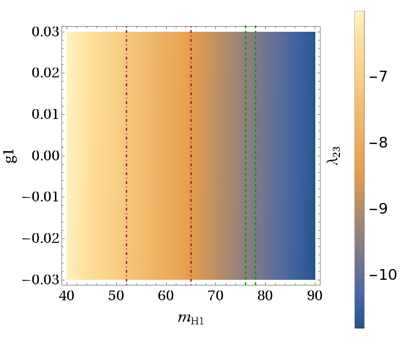
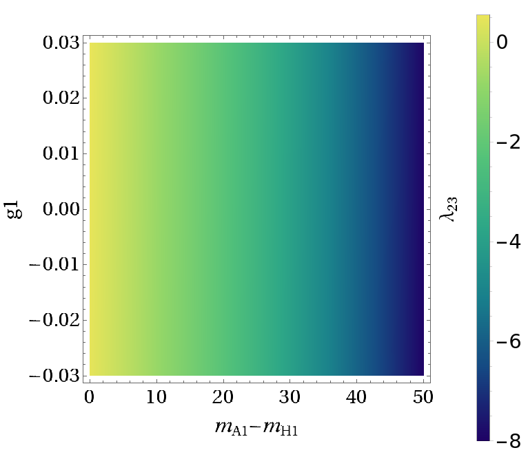
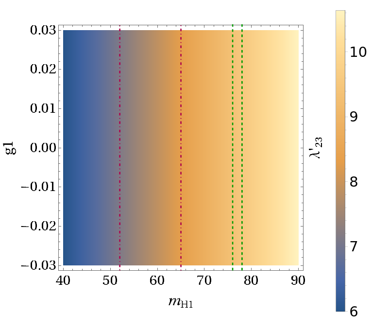
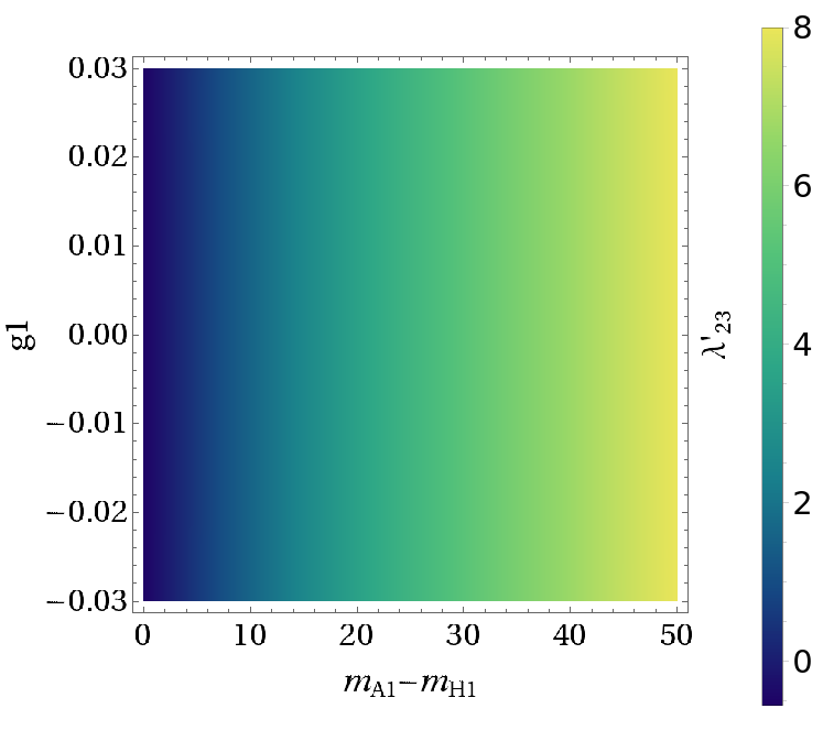
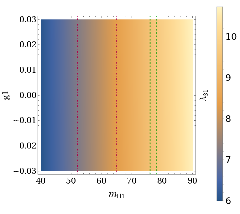
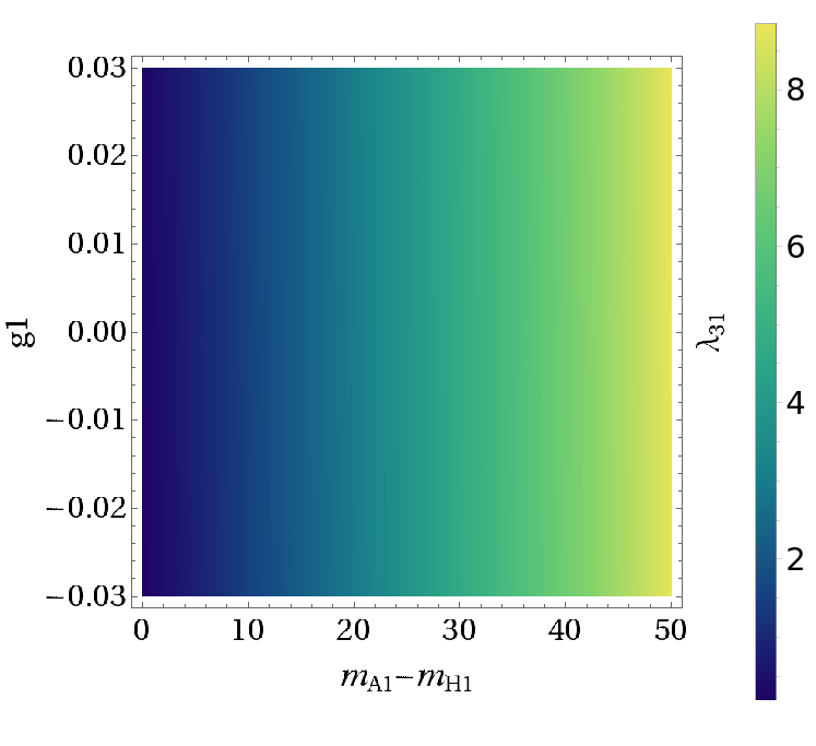
Figure 1: Scan on the $\lambda^{(\prime)}$ parameters, for $0\leq\mu_{12}\leq 63$ GeV. On the left, the scan is shown as a function of $g_{1}$ and $m_{H_{1}}$ with $40$ GeV$\leq m_{H_{1}}\leq 90$ GeV, wherein the dotted lines show the intervals for $m_{H_{1}}$ that satisfy the experimental and theoretical restrictions. On the right, the scan is shown as a function of $g_{1}$ and $\Delta_{h}(=m_{A_{1}}-m_{H_{1}})$ with $0\leq m_{A_{1}}-m_{H_{1}}\leq 50$ GeV.

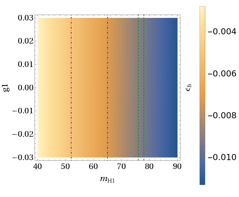
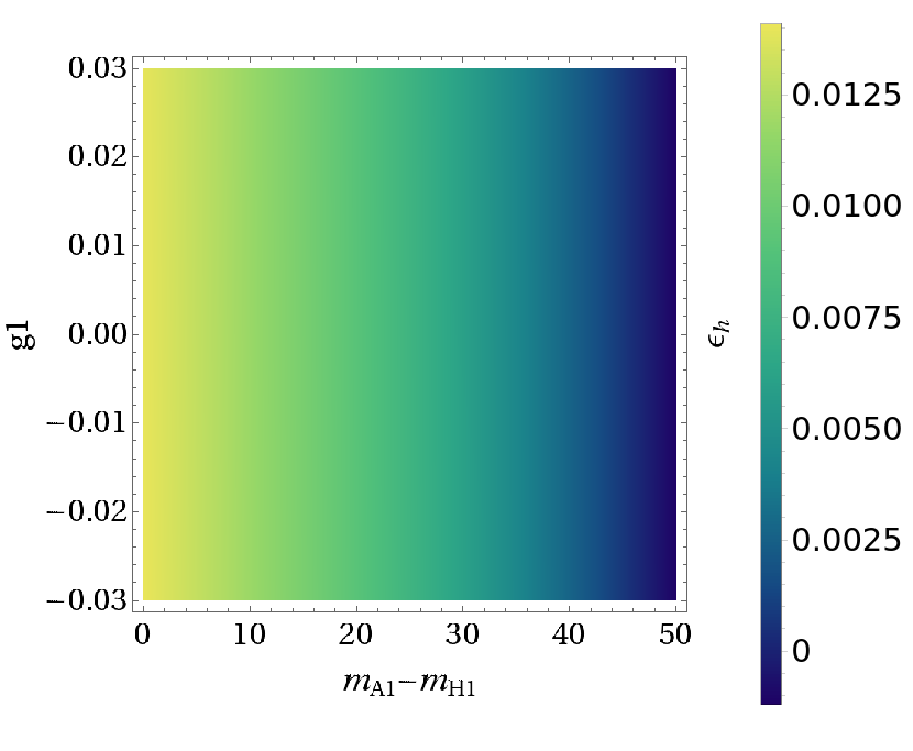
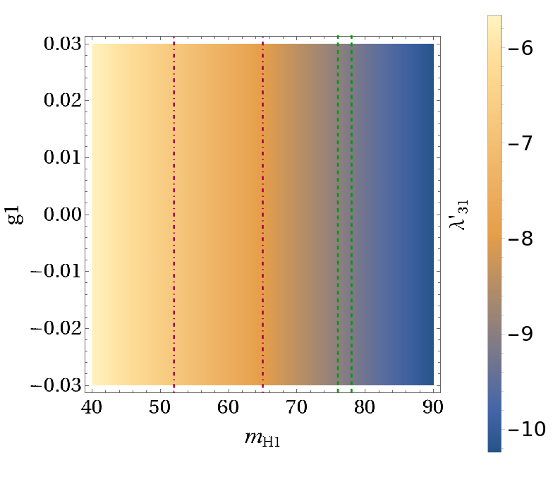
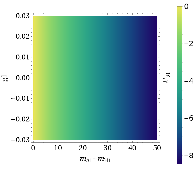
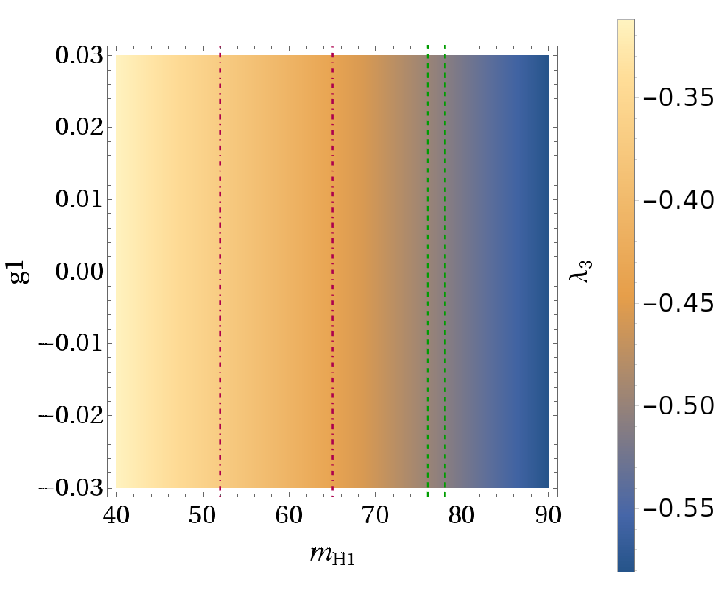
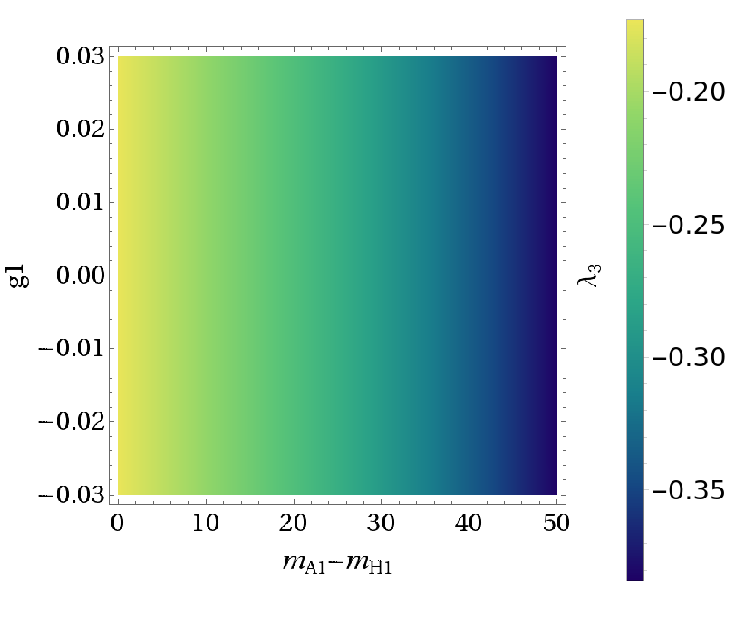
Figure 2: Scan on the $\lambda^{(\prime)}$ parameters and $\epsilon_{n}$, for $0\leq\mu_{12}\leq 63$ GeV. On the left, the scan is shown as a function of $g_{1}$ and $m_{H_{1}}$ with $40$ GeV$\leq m_{H_{1}}\leq 90$ GeV, wherein the dotted lines show the intervals for $m_{H_{1}}$ that satisfy experimental and theoretical restrictions. On the right, the scan is shown as a function of $g_{1}$ and $\Delta_{h}(=m_{A_{1}}-m_{H_{1}})$ with $0\leq m_{A_{1}}-m_{H_{1}}\leq 50$ GeV.

Table 1: Input values for the parameter space scans in Figs. 1–2.

Parameters
$40$ GeV$\leq m_{H_{1}}\leq 90$ GeV
$\Delta_{h}=m_{A_{1}}-m_{H_{1}}=50$ GeV
$\Delta_{c}=m_{H_{1}^{\pm}}-m_{H_{1}}=60$ GeV
$\delta_{c}=m_{H_{2}^{\pm}}-m_{H_{1}^{\pm}}=10$ GeV
$0.005\leq g_{1}\leq 0.02$ and $g_{2}=-0.13$
$0\leq\mu_{12}\leq 63$ GeV

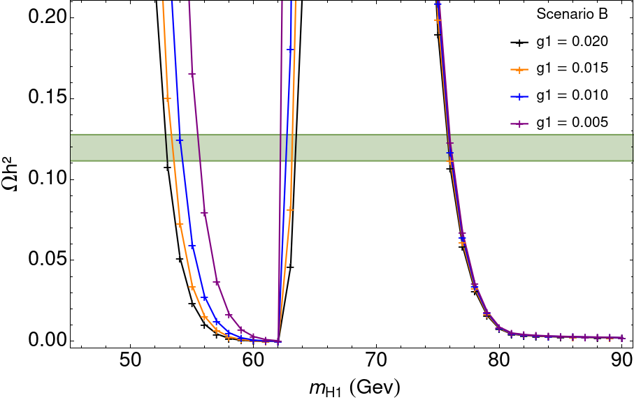
Figure 3: The combined relic density of the DM constituents $H_{1}$ and $A_{1}$ with respect to $m_{H_{1}}$ in scenario B given as lines for discrete values of a positive $g_{1}$ coupling. The gray band represents the values for relic density that satisfy all constrains including direct and indirect detection as well as invisible decays.

Table 2: Input values for the parameter space scan in Fig. 3.

Parameters			scenario B
$\lambda_{11}=0.13$	$\lambda^{\prime}_{12}=0.12$	$-0.029\leq g_{1}\leq 0.029$	$m_{H_{2}}-m_{A_{2}}=$ 30 GeV
$\lambda_{22}=0.11$	$\lambda_{1}=0.1$	$-0.2<g_{2}<0.2$	$\Delta_{c}=$60 GeV
$\lambda_{12}=0.12$		$-0.1<\lambda_{2}<0.1$	$\delta_{c}=$10 GeV
		$\Delta_{n}=m_{A_{2}}-m_{H_{1}}$	$m_{A_{1}}-m_{H_{1}}=50$ GeV
		$\Delta_{n^{\prime}}=m_{H_{2}}-m_{A_{1}}$	$g_{2}=-0.13$
		$50$ GeV $<\Delta_{n}<100$ GeV	$\lambda_{2}=0.1$

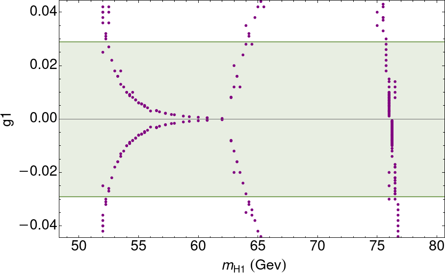
Figure 4: The combined relic density of the DM constituents with respect to $m_{H_{1}}$ in scenario B given as points for continuous values of the $g_{1}$ coupling. The gray band represents the values for relic density that satisfy all constrains including direct and indirect detection as well as invisible decays.

IV Numerical results

Since the Hermaphrodite DM states $H_{1}$ and $A_{1}$ are protected from decaying into SM particles by the conservation of $Z_{3}$ symmetry, the two particles are stable in this model. According to Eqs. (14)–(15) and (20), $m_{H_{1}}<m_{A_{1}}<m_{A_{2}}<m_{H_{2}}$. The heavier particles, $A_{2}$ and $H_{2}$, are unstable and their decays in $H_{1}$, $A_{1}$ or SM particles could provide experimental signals. We focus our study on the production of DM, considering the following processes: $pp\to 2l+2{\rm DM}$ for the current LHC machine (see the Feynman diagrams in Fig. 5) and $e^{+}e^{-}\to 2l+2{\rm DM}$ for a future electron-positron accelerator (see the Feynman diagrams in Fig. 6), wherein $l(\bar{l})=e^{+}(e^{-}),\mu^{+}(\mu^{-})$ and ${\rm DM}=H_{1},A_{1}$. (Hereafter, we use the notation $2l$ for short, to signify an electron or muon pair of opposite charge.) The leading diagrams are those where the vertices $ZA_{1}H_{2}$ and $ZA_{2}H_{1}$ appear. The aforementioned processes to obtain DM particles also involve decays of the $Z$ boson and the $h$ state. As mentioned, we take the scalar field $h$ to the SM-like Higgs boson, hence $m_{h}=125$ GeV. As for the $H_{i},A_{i}$ dark states, we will select a few BPs from the available parameter space that we have isolated. Finally, MadGraph will be used for our calculations at the parton level [19] with integrated and differential distributions obtained via MadAnalysis [20].

Figure 5: Feynman diagrams for the processes $pp\to 2l+2{\rm DM}$, where $q=u,d$, $\bar{q}=\bar{u},\bar{d}$, $l=e^{-}(\mu^{-})$ and $\bar{l}=e^{+}(\mu^{+})$, $H_{s}=A_{2}(H_{2})$ and ${\rm DM}=H_{1}(A_{1})$. The first diagram is the leading one.

Figure 6: Feynman diagrams for the processes $e^{+}e^{-}\to 2l+2{\rm DM}$, where $l=e^{-}(\mu^{-})$ and $\bar{l}=e^{+}(\mu^{+})$, $H_{s}=A_{2}(H_{2})$ and ${\rm DM}=H_{1}(A_{1})$. The first and last diagrams are the leading ones. (The diagrams in the second row only enter for the case $l=e^{-}$ and $\bar{l}=e^{+}$.)

IV.1 LHC signatures $pp\to 2l+2H_{1}(2A_{1})$

For the LHC machine, we consider the following signature: $2l+\cancel{E}_{T}$ (where $\cancel{E}_{T}$ is the missing $E_{T}$ of the event), which can be induced at tree-level by the processes $pp\to 2l+2H_{1}(2A_{1})$. In our analysis, the following basics cuts on leptons are considered: transverse momentum $p_{T}(l)>10$ GeV, pseudorapidity $|\eta(l)|<2.5$ and separation $\Delta R(l^{+},l^{-})>0.4$. We take one BP within scenario B (with $\Delta_{n(n^{\prime})}=70(50)$ GeV), which is identified by the following mass and coupling parameter values: $m_{H_{1}}=53$ GeV, $m_{A_{1}}=103$ GeV, $m_{A_{2}}=123$ GeV, $m_{H_{2}}=153$ GeV and $g_{1}=0.029$. Since the mass difference $\Delta_{h}=m_{A_{1}}-m_{H_{1}}$ is taken larger than the detector resolution in $\cancel{E}_{T}$ as well as in mass variables (e.g., invariant, $M(l^{+}l^{-})$, or transverse, $M_{T}(l^{+}l^{-})$) involving leptons (and $\cancel{E}_{T}$) at the LHC, we could then observe the presence of both Hermaphrodite DM components simultaneously. For this BP of scenario B, we show in Tab. 3 both cross-sections and event rates at partonic level, assuming $\sqrt{s}_{pp}=14$ TeV and a luminosity of $L=100$ fb^-1, which could be accrued within a few years of operation at the LHC during Run 3. In general, the value of the cross-section $\sigma(pp\to 2l+2H_{1}(2A_{1}))$ depends mostly on the mass difference $\Delta_{n}=m_{A_{2}}-m_{H_{1}}$ ($\Delta_{n^{\prime}}=m_{H_{2}}-m_{A_{1}}$), which is thus very important in the description of the distributions generated.

Table 3: Cross-section for the processes $pp\to 2l+2{\rm DM}$, with ${\rm DM}=H_{1},A_{1}$, taking $L=100$ fb^-1 as well as $m_{H_{1}}=53$ GeV, $m_{A_{1}}=103$ GeV, $m_{A_{2}}=123$ GeV, $m_{H_{2}}=153$ GeV, $g_{1}=0.029$ with other parameters as in scenario B.

DM	$\sigma(pp\to 2l+2{\rm DM})$	Event rates
$H_{1}$	0.280 pb	$2.8\times 10^{4}$
$A_{1}$	0.135 pb	$1.35\times 10^{4}$

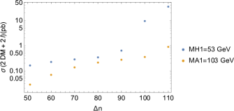
Figure 7: Cross-section of the processes $pp\to 2l+2H_{1}$ (blue colour) and $pp\to 2l+2A_{1}$ (orange colour) as a function of $\Delta_{n}=m_{A_{2}}-m_{H_{1}}$ (in GeV), with $m_{A_{1}}=103$ GeV and $m_{H_{1}}=53$ GeV. All points are compliant with DM (in)direct detection bounds and relic density as well as the Higgs to invisible BR constraint. Here, $\sqrt{s}_{pp}=14$ TeV.

In Fig. 7, we show the behaviour of the cross-section $\sigma(pp\to 2l+2H_{1}(2A_{1}))$ versus the $\Delta_{n}=m_{A_{2}}-m_{H_{1}}$ parameter, the points in blue colour being for $H_{1}$ and the points in orange colour being for $A_{1}$. One can see that, in the region 70 GeV $\leq\Delta_{n}\leq 90$ GeV, the cross-sections for $H_{1}$ and $A_{1}$ are closest to each other. A small relative rate, alongside a sufficiently large absolute value of either $\sigma$, is a precondition to observe the two Hermaphrodite candidates simultaneously. Hence, our BP is taken in this range, in particular, with $\Delta_{n}=70$ GeV, so that the events rates for the two DM processes are within the same order of magnitude (see Tab. 3).

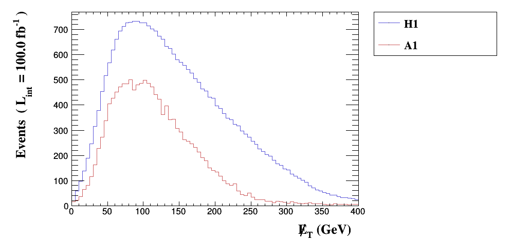
Figure 8: Spectra in missing transverse energy (left) and transverse momentum of each lepton (right) for the processes $pp\to 2l+2{\rm DM}$, where the distributions are identified by a blue colour line for ${\rm DM}=H_{1}$ and a red colour line for ${\rm DM}=A_{1}$. These correspond to scenario B with the specific choices $\Delta_{n}=m_{A_{2}}-m_{H_{1}}=70$ GeV and $\Delta_{n^{\prime}}=m_{H_{2}}-m_{A_{1}}=50$ GeV.

Following such a choice, in Fig. 8, we obtain rather similar shapes in the distributions of the missing transverse energy $\cancel{E}_{T}$ and transverse momentum of each lepton $p_{T}(l)$.

Figure 9: Spectra in pseudorapidity of each lepton (left) and relative distance between leptons (right) for the processes $pp\to 2l+2{\rm DM}$, where the distributions are identified by a blue colour line for ${\rm DM}=H_{1}$ and a red colour line for ${\rm DM}=A_{1}$. These correspond to scenario B with the specific choices $\Delta_{n}=m_{A_{2}}-m_{H_{1}}=70$ GeV and $\Delta_{n^{\prime}}=m_{H_{2}}-m_{A_{1}}=50$ GeV.

Figure 10: Spectra in invariant mass of the leptons for the processes $pp\to 2l+2{\rm DM}$, where the distributions are identified by a blue colour line for ${\rm DM}=H_{1}$ and a red colour line for ${\rm DM}=A_{1}$. These correspond to scenario B with the specific choices $\Delta_{n}=m_{A_{2}}-m_{H_{1}}=70$ GeV and $\Delta_{n^{\prime}}=m_{H_{2}}-m_{A_{1}}=50$ GeV.

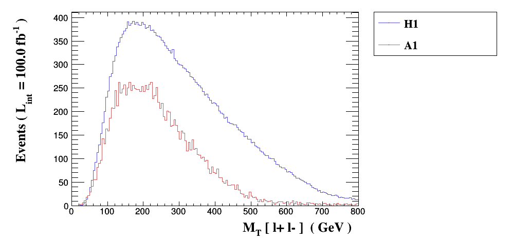
Figure 11: Spectra in transverse mass of the final state for the processes $pp\to 2l+2{\rm DM}$, where the distributions are identified by a blue colour line for ${\rm DM}=H_{1}$ and a red colour line for ${\rm DM}=A_{1}$. These correspond to scenario B with the specific choices $\Delta_{n}=m_{A_{2}}-m_{H_{1}}=70$ GeV and $\Delta_{n^{\prime}}=m_{H_{2}}-m_{A_{1}}=50$ GeV.

Likewise, in Fig. 9, one can see that also the pseudorapidity of each lepton $\eta(l)$ and separation between them $\Delta R(l^{+}l^{-})$ have rather similar shapes. As the last three variables are used for selection purposes, we would conclude that our envisaged cutflow would not dramatically change the relative rates seen in Tab. 3. Unfortunately, though, the $\cancel{E}_{T}$ spectrum cannot afford one with separating the $H_{1}$ and $A_{1}$ components of Hermaphrodite DM. However, this would become possible for the case of the invariant mass of the di-lepton system, as seen in Fig. 10, wherein the off-shell $Z$ large peaks for $H_{1}$ and $A_{1}$ are separately visible and can strongly be correlated to the values of $\Delta_{n}$ and $\Delta_{n^{\prime}}$, respectively. (Also, notice the small on-shell $Z$ peaks for both DM candidates.) In contrast, the transverse mass distribution $M_{T}^{2}(l^{+}l^{-})=(\sum_{i}^{l^{+},l^{-}}E_{Ti})^{2}-(\sum_{i}^{l^{+},l^{-}}p_{Ti})^{2}$, wherein the proton beams are along the $z$-axis, shown in Fig. 11 offers one little chance to pinpoint the presence of Hermaphrodite DM.

IV.2 Electron-positron collider processes $e^{+}e^{-}\to 2l+2H_{1}(2A_{1})$

We here analyse the signature $2l+\cancel{E}_{T}$ at a future electron-positron machine, which is induced by the processes $e^{+}e^{-}\to 2l+2H_{1}(2A_{1})$. In order to demonstrate how to probe our scenario across two different collider environments, we utilise the same model configuration as in the LHC analysis of the previous section, so we select scenario B with the same choice of $\Delta_{n}$ and $\Delta_{n^{\prime}}$ (for the kinematical analysis). As possible energies of a future $e^{+}e^{-}$ collider, we adopt $\sqrt{s}_{ee}=250$, 350, 500 and 1000 GeV, with $L=1000$ fb^-1 in all cases. We also assume the following beam polarisations: 80% for the $e^{-}$ beam and 30% for the $e^{+}$ beam, though neither of these is necessary to uphold our forthcoming conclusions. Cuts are the same as in the LHC case (initially). Again, as it happened for the latter, the cross-sections at an $e^{+}e^{-}$ machine depend on the mass splitting $m_{A_{2}}-m_{H_{1}}$ for the $e^{+}e^{-}\to 2l+2H_{1}$ channel and on $m_{H_{2}}-m_{A_{1}}$ for the channel $e^{+}e^{-}\to 2l+2A_{1}$. Indeed, at a future $e^{+}e^{-}$ machine, the detector resolution is even better than at the LHC, so we expect to be able to see the two DM components of our $Z_{3}$ symmetric I(2+1)HDM scenario even more strikingly. To start with, Fig. 12 illustrates that, at the inclusive level, production rates of the above two processes are extremely significant, so the conditions are now much more favourable than the hadron machine. (Here, we have shown rates for the $H_{1}$ case, but they are overall similar for the $A_{1}$ one.) Furthermore, Fig. 13 illustrates that no matter the value of $e^{+}e^{-}$ collider energy, our choice of the BP within scenario B complies only somewhat with the aforementioned conditions for the total and relative rates of the cross-sections corresponding to the DM candidates while Tab. 4 shows their actual values at $\sqrt{s}=500$ GeV, the energy configuration that we adopt for the forthcoming kinematic analysis. By investigating the usual distributions in $\cancel{E}_{T}$, $p_{T}(l)$, $\eta(l)$ and $\Delta R(l^{+},l^{-})$, see Figs. 14–15, it is clear that their shapes are rather different for the two Hermaphrodite DM contributions, owing to the fact that the collider energy chosen is more comparable to the inert (pseudo)scalar masses than that of the LHC. However, they are such that the $A_{1}$ component is always subleading with respect to the $H_{1}$ one. In fact, even the $M(l^{+}l^{-})$ distribution, Fig. 16, where the two contributions are very different (primarily because of a large on-shell $Z$ contribution in the $H_{1}$ case which is absent in the $A_{1}$ one), would not afford one to separate them.

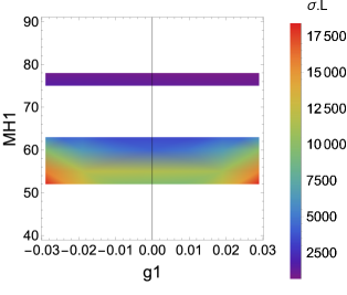
Figure 12: Event rates of the process $e^{+}e^{-}\to 2l+2H_{1}$ as a function of $g_{1}$ and $M_{H_{1}}$ for $\sqrt{s}_{ee}=250$ GeV and $L=1000$ fb^-1 over the parameter space corresponding to scenario B in Tab. 2. All points are compliant with DM (in)direct detection bounds and relic density as well as the Higgs to invisible BR constraint. (The most optimistic BP is for $m_{H_{1}}=53$ GeV and $g_{1}=-0.029$, where the cross-section is $\sigma=16.01$ fb.)

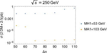
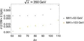
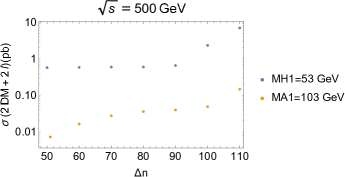
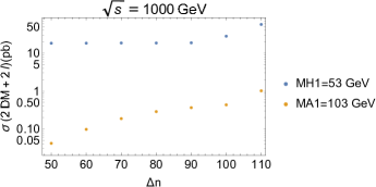
Figure 13: Cross-section of the processes $e^{+}e^{-}\to 2l+2H_{1}$ (blue colour) and $e^{+}e^{-}\to 2l+2A_{1}$ (orange colour) as a function of $\Delta_{n}=m_{A_{2}}-m_{H_{1}}$ (in GeV), with $m_{A_{1}}=103$ GeV and $m_{H_{1}}=53$ GeV. All points are compliant with DM (in)direct detection bounds and relic density as well as the Higgs to invisible BR constraint. Here, $\sqrt{s}_{ee}=250$ (top-left), 350 (top-right), 500 (bottom-left) and 1000 (bottom-right) GeV.

Table 4: Cross-section for the processes $e^{+}e^{-}\to 2l+2{\rm DM}$, with ${\rm DM}=H_{1},A_{1}$, taking $L=1000$ fb^-1 as well as $m_{H_{1}}=53$ GeV, $m_{A_{1}}=103$ GeV, $m_{A_{2}}=123$ GeV, $m_{H_{2}}=153$ GeV, $g_{1}=0.029$ with other parameters as in scenario B.

DM	$\sigma(e^{+}e^{-}\to 2l+2{\rm DM})$	Event rates
$H_{1}$	0.586 pb	$5.86\times 10^{5}$
$A_{1}$	0.027 pb	$2.7\times 10^{4}$

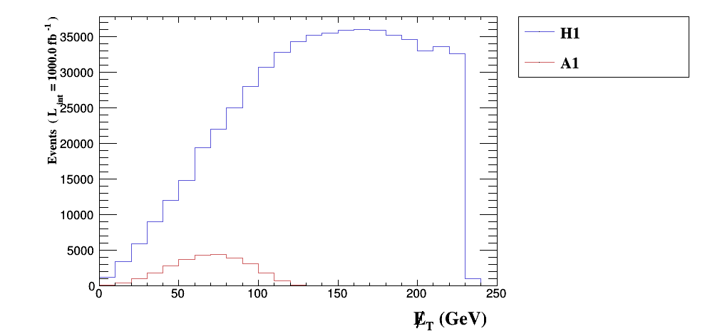
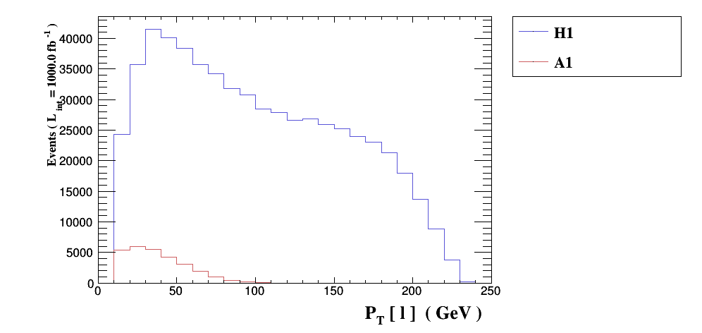
Figure 14: Spectra in missing transverse energy (left) and transverse momentum of each lepton (right) for the processes $e^{+}e^{-}\to 2l+2{\rm DM}$, where the distributions are identified by a blue colour line for ${\rm DM}=H_{1}$ and a red colour line for ${\rm DM}=A_{1}$. These correspond to scenario B with the specific choices $\Delta_{n}=m_{A_{2}}-m_{H_{1}}=70$ GeV and $\Delta_{n^{\prime}}=m_{H_{2}}-m_{A_{1}}=50$ GeV.

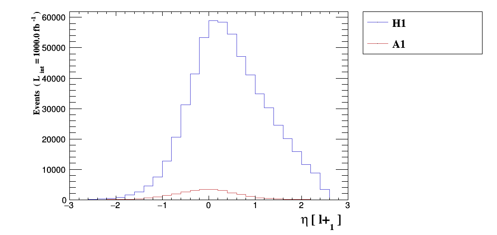
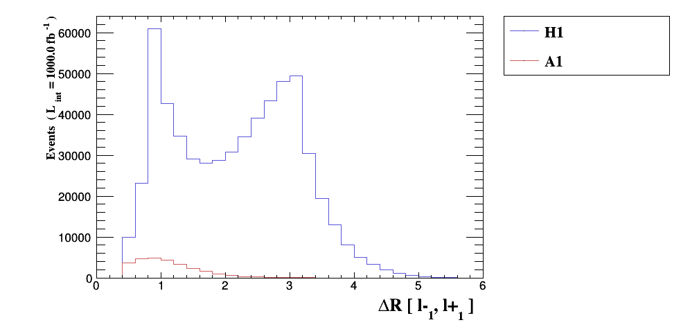
Figure 15: Spectra in pseudorapidity of each lepton (left) and relative distance between leptons (right) for the processes $pp\to 2l+2{\rm DM}$, where the distributions are identified by a blue colour line for ${\rm DM}=H_{1}$ and a red colour line for ${\rm DM}=A_{1}$. These correspond to scenario B with the specific choices $\Delta_{n}=m_{A_{2}}-m_{H_{1}}=70$ GeV and $\Delta_{n^{\prime}}=m_{H_{2}}-m_{A_{1}}=50$ GeV.

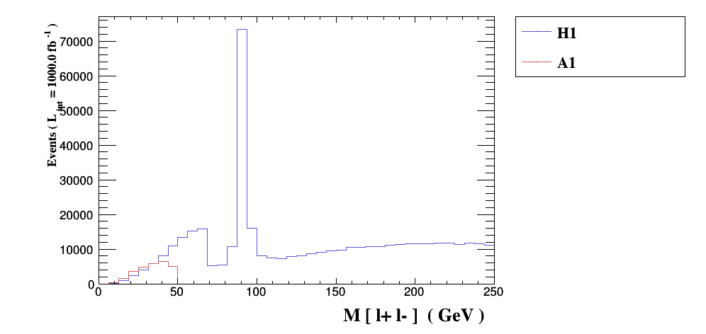
Figure 16: Spectra in invariant mass of the leptons for the processes $e^{+}e^{-}\to 2l+2{\rm DM}$, where the distributions are identified by a blue colour line for ${\rm DM}=H_{1}$ and a red colour line for ${\rm DM}=A_{1}$. These correspond to scenario B with the specific choices $\Delta_{n}=m_{A_{2}}-m_{H_{1}}=70$ GeV and $\Delta_{n^{\prime}}=m_{H_{2}}-m_{A_{1}}=50$ GeV.

Therefore, it is appropriate to enforce some additional cuts, in order to make the two cross-sections for $H_{1}$ and $A_{1}$ more comparable. By inspecting Figs. 14–15, we choose the phase space regions where $\cancel{E}_{T}<120$ GeV and $\Delta R(l,l)<1.4$. In the presence of these additional selections, it becomes clear that the two Hermaphrodite DM contributions become similar in normalisation while retaining sufficiently different shapes so to allow one to attempt their extraction, in both the invariant mass spectrum of the di-lepton pair (Fig. 17) and transverse mass of the final state (Fig. 18).

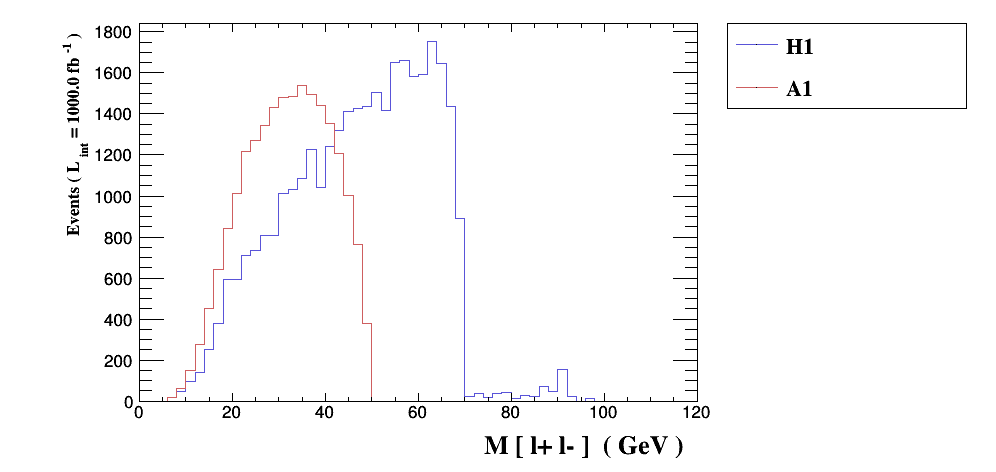
Figure 17: Spectra in invariant mass of the leptons for the processes $e^{+}e^{-}\to 2l+2{\rm DM}$, where the distributions are identified by a blue colour line for ${\rm DM}=H_{1}$ and a red colour line for ${\rm DM}=A_{1}$. These correspond to scenario B with the specific choices $\Delta_{n}=m_{A_{2}}-m_{H_{1}}=70$ GeV and $\Delta_{n^{\prime}}=m_{H_{2}}-m_{A_{1}}=50$ GeV. Here, we include the additional cuts in $\cancel{E}_{T}$ and $\Delta R(l^{+},l^{-})$.

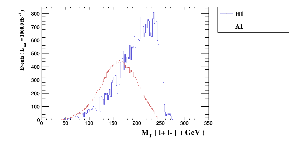
Figure 18: Spectra in transverse mass of the final state for the processes $e^{+}e^{-}\to 2l+2{\rm DM}$, where the distributions are identified by a blue colour line for ${\rm DM}=H_{1}$ and a red colour line for ${\rm DM}=A_{1}$. These correspond to scenario B with the specific choices $\Delta_{n}=m_{A_{2}}-m_{H_{1}}=70$ GeV and $\Delta_{n^{\prime}}=m_{H_{2}}-m_{A_{1}}=50$ GeV. Here, we include the additional cuts in $\cancel{E}_{T}$ and $\Delta R(l^{+},l^{-})$.

V Conclusions

In this paper, we have studied a realisation of the 3HDM, wherein one doublet is active, and two are inert (hence it is termed I(2+1)HDM), which, in the presence of a softly broken $Z_{3}$ symmetry, yields two DM candidates, in the form of the lightest CP-even and CP-odd states from the inert sector, $H_{1}$ and $A_{1}$, respectively. These two states, emerging from the same sector (hence with the same $Z_{3}$ properties), while having opposite CP quantum numbers, are not mass degenerate and have different gauge couplings, so that they cannot be ascribed to being the real and imaginary part of a single complex field. Therefore, they have been called Hermaphrodite DM. In the presence of constraints coming from the theoretical and experimental side, we have been able to isolate an expanse of I(2+1)HDM parameter space over which the two states $H_{1}$ and $A_{1}$ are at the EW scale with a mass separation of order 50 GeV. As the next-to-lightest CP-odd and CP-even states from the inert sector, $A_{2}$ and $H_{2}$, respectively, can decay into the DM candidates via a $Z$ boson, we have pursued here some possible signals of such Hermaphrodite DM, consisting of $2l+\cancel{E}_{T}$ final states, which can be produced at both the LHC and a future electron-positron collider. In the first case, the hard process involved is $q\bar{q}\to Z\to 2l2H_{1}(2A_{1})$ whereas in the second case this is $e^{+}e^{-}\to Z\to 2l2H_{1}(2A_{1})$. The fact that the two Hermaphrodite DM states have a common final state enables one to potentially see these simultaneously in differential distributions that would have a distinctive shape carrying the imprint of the two underlying components, each corresponding to a different DM candidate, at both the hadron and lepton collider. We have proven this to be the case for several observables by using a parton-level MC analysis, albeit without a signal-to-background study. Therefore, we encourage experimentalists to look into this I(2+1)HDM hallmark phenomenology, as it would manifest itself in one of the most studied final states at both the aforementioned machines. Altogether, we expect that some evidence of two-component Hermaphrodite DM could first be seen at the LHC and eventually be characterised at a future $e^{+}e^{-}$ collider.

References

References

• Aad et al. [2012] G. Aad et al. (ATLAS), Observation of a new particle in the search for the Standard Model Higgs boson with the ATLAS detector at the LHC, Phys. Lett. B 716, 1 (2012), arXiv:1207.7214 [hep-ex] .
• Chatrchyan et al. [2012] S. Chatrchyan et al. (CMS), Observation of a New Boson at a Mass of 125 GeV with the CMS Experiment at the LHC, Phys. Lett. B 716, 30 (2012), arXiv:1207.7235 [hep-ex] .
• Barger et al. [1990] V. D. Barger, J. L. Hewett, and R. J. N. Phillips, New Constraints on the Charged Higgs Sector in Two Higgs Doublet Models, Phys. Rev. D 41, 3421 (1990).
• Grossman [1994] Y. Grossman, Phenomenology of models with more than two Higgs doublets, Nucl. Phys. B 426, 355 (1994), arXiv:hep-ph/9401311 .
• Aoki et al. [2009] M. Aoki, S. Kanemura, K. Tsumura, and K. Yagyu, Models of Yukawa interaction in the two Higgs doublet model, and their collider phenomenology, Phys. Rev. D 80, 015017 (2009), arXiv:0902.4665 [hep-ph] .
• Deshpande and Ma [1978] N. G. Deshpande and E. Ma, Pattern of Symmetry Breaking with Two Higgs Doublets, Phys. Rev. D 18, 2574 (1978).
• Aranda et al. [2021a] A. Aranda, D. HernĂĄndez-Otero, J. HernĂĄndez-Sanchez, V. Keus, S. Moretti, D. Rojas-Ciofalo, and T. Shindou, $Z_{3}$ symmetric inert ( 2+1 )-Higgs-doublet model, Phys. Rev. D 103, 015023 (2021a), arXiv:1907.12470 [hep-ph] .
• Ivanov et al. [2012] I. P. Ivanov, V. Keus, and E. Vdovin, Abelian symmetries in multi-Higgs-doublet models, Journal of Physics A: Mathematical and Theoretical 45, 215201 (2012).
• Aranda et al. [2021b] A. Aranda, D. HernĂĄndez-Otero, J. HernĂĄndez-Sanchez, V. Keus, S. Moretti, D. Rojas-Ciofalo, and T. Shindou, $Z_{3}$ symmetric inert (2+1)-Higgs-doublet model, Physical Review D 103 (2021b).
• Keus et al. [2014] V. Keus, S. F. King, and S. Moretti, Phenomenology of the inert (2+1) and (4+2) Higgs doublet models, Physical Review D 90 (2014).
• Cao et al. [2007] Q.-H. Cao, E. Ma, and G. Rajasekaran, Observing the dark scalar doublet and its impact on the standard-model Higgs boson at colliders, Physical Review D 76 (2007).
• Lundström et al. [2009] E. Lundström, M. Gustafsson, and J. Edsjö, Inert doublet model and LEP II limits, Physical Review D 79 (2009).
• Aaboud et al. [2019] M. Aaboud, G. Aad, B. Abbott, D. Abbott, O. Abdinov, A. Abed Abud, D. Abhayasinghe, S. Abidi, O. AbouZeid, N. Abraham, and et al., Combination of Searches for Invisible Higgs Boson Decays with the ATLAS Experiment, Physical Review Letters 122 (2019).
• Cordero-Cid et al. [2020] A. Cordero-Cid, J. HernĂĄndez-SĂĄnchez, V. Keus, S. Moretti, D. Rojas, and D. SokoƂowska, Lepton collider indirect signatures of dark CP-violation, The European Physical Journal C 80 (2020).
• Aghanim et al. [2020] N. Aghanim, Y. Akrami, M. Ashdown, J. Aumont, C. Baccigalupi, M. Ballardini, A. J. Banday, R. B. Barreiro, N. Bartolo, and et al., Planck 2018 results, Astronomy & Astrophysics 641, A6 (2020).
• Aprile et al. [2018] E. Aprile, J. Aalbers, F. Agostini, M. Alfonsi, L. Althueser, F. Amaro, M. Anthony, F. Arneodo, L. Baudis, B. Bauermeister, and et al., Dark Matter Search Results from a One Ton-Year Exposure of XENON1T, Physical Review Letters 121 (2018).
• Karwin et al. [2017] C. Karwin, S. Murgia, T. M. Tait, T. A. Porter, and P. Tanedo, Dark matter interpretation of the Fermi-LAT observation toward the Galactic Center, Physical Review D 95 (2017).
• BĂ©langer et al. [2014] G. BĂ©langer, F. Boudjema, A. Pukhov, and A. Semenov, micrOMEGAs3.1: A program for calculating dark matter observables, Computer Physics Communications 185, 960 (2014).
• Alwall et al. [2014] J. Alwall, R. Frederix, S. Frixione, V. Hirschi, F. Maltoni, O. Mattelaer, H. S. Shao, T. Stelzer, P. Torrielli, and M. Zaro, The automated computation of tree-level and next-to-leading order differential cross sections, and their matching to parton shower simulations, JHEP 07, 079, arXiv:1405.0301 [hep-ph] .
• Conte et al. [2013] E. Conte, B. Fuks, and G. Serret, MadAnalysis 5, A User-Friendly Framework for Collider Phenomenology, Comput. Phys. Commun. 184, 222 (2013), arXiv:1206.1599 [hep-ph] .