Towards Equal Opportunity Fairness through Adversarial Learning

Abstract

Adversarial training is a common approach for bias mitigation in natural language processing. Although most work on debiasing is motivated by equal opportunity, it is not explicitly captured in standard adversarial training. In this paper, we propose an augmented discriminator for adversarial training, which takes the target class as input to create richer features and more explicitly model equal opportunity. Experimental results over two datasets show that our method substantially improves over standard adversarial debiasing methods, in terms of the performance–fairness trade-off.

1 Introduction

While natural language processing models have achieved great successes across a variety of classification tasks in recent years, naively-trained models often learn spurious correlations with confounds like user demographics and socio-economic factors (Badjatiya et al., 2019; Zhao et al., 2018; Li et al., 2018a).

A common way of mitigating bias relies on “unlearning” discriminators during the debiasing process. For example, in adversarial training, an encoder and discriminator are trained such that the encoder attempts to prevent the discriminator from identifying protected attributes (Zhang et al., 2018; Li et al., 2018a; Han et al., 2021c). Intuitively, such debiased representations from different protected groups are not separable, and as a result, any classifier applied to debiased representations will also be agnostic to the protected attributes. The fairness metric corresponding to such debiasing methods is known as demographic parity (Feldman et al., 2015), which is satisfied if classifiers are independent of the protected attribute. Taking loan applications as an example, demographic parity is satisfied if candidates from different groups have the same approval rate.

However, demographic parity has its limitations, as illustrated by Barocas et al. (2019): a hirer that carefully selects applicants from group $a$ and arbitrarily selects applicants from group $b$ with the same acceptance rate of $p>0$ achieves demographic parity, but is far from fair as they are more likely to select inappropriate applicants in group $b$.

In acknowledgement of this issue, (Hardt et al., 2016) proposed: (1) equalized odds, which is satisfied if a classifier is independent of protected attributes within each class, i.e., class-specific independent; and (2) equal opportunity, which is a relaxed version of equalized odds that only focuses on independence in “advantaged” target classes (such as the approval class for loans).

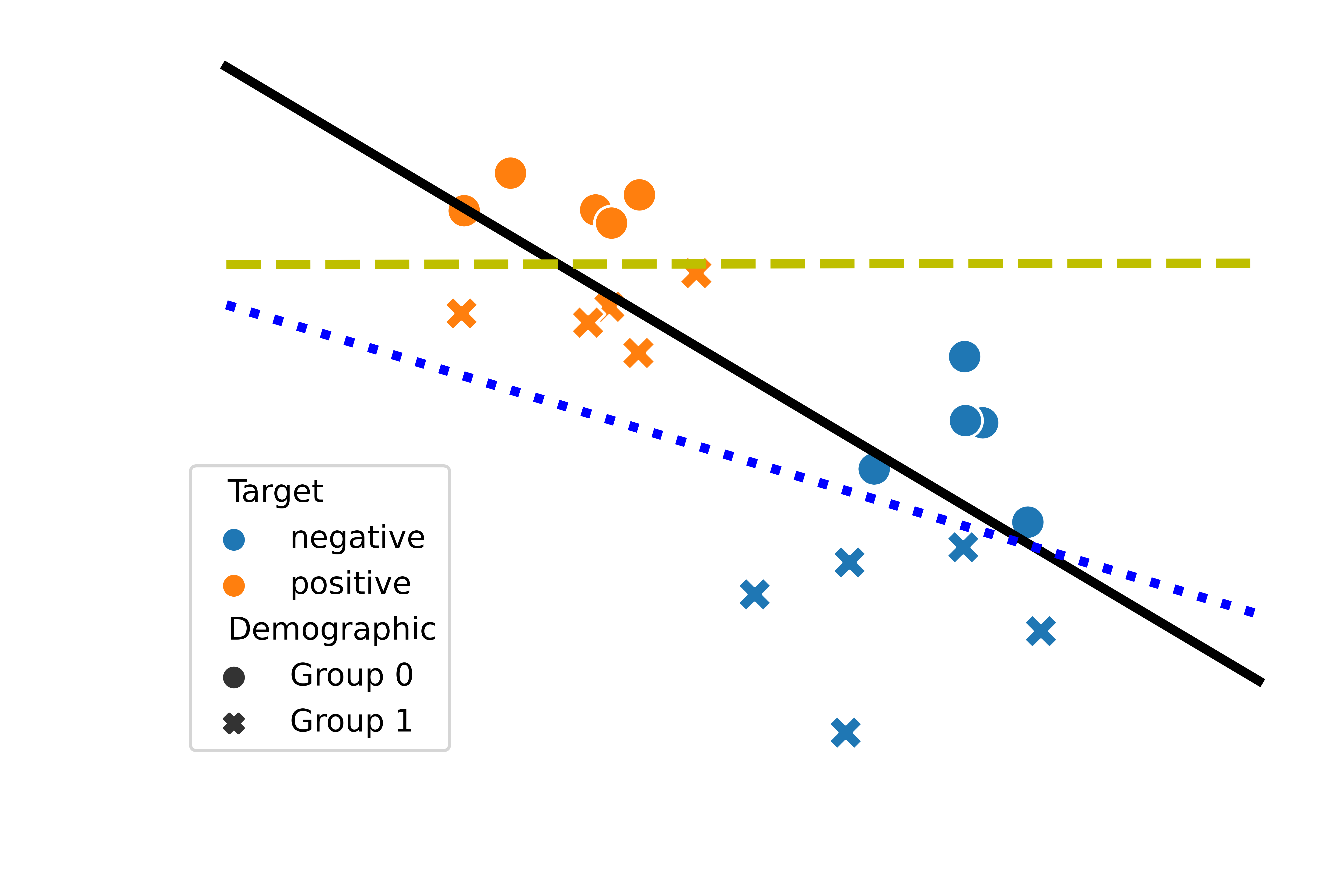
Figure 1: The black solid, yellow dashed, and blue dotted lines are the decision boundaries of linear discriminators for demographic trained over all instances, $\mathbf{y}=$ positive, and $\mathbf{y}=$ negative, resp. The decision boundaries learned by our proposed class-specific discriminators (yellow ashed and blue dotted) are distinct to the previous discriminator setting (black solid).

Similar to demographic parity, standard adversarial training does not consider the target label for protected information removal, which is fundamental to equal opportunity. Figure 1 shows a toy example where hidden representations are labelled with the associated target labels via colour, and protected labels via shape. Taking the target label information into account and training separate discriminators for each of the two protected attributes, it can be seen that the linear decision boundaries are quite distinct, and each is different from the decision boundary when the target class is not taken into consideration.

To enable adversarial training to recognize the correlation between protected attributes and target classes, we propose a novel discriminator architecture that captures the class-specific protected attributes during adversarial training. Moreover, our proposed mechanism is generalizable to other SOTA variants of adversarial training, such as DAdv (Han et al., 2021c). Experiments over two datasets show that our method consistently outperforms standard adversarial learning.

The source code has been included in fairlib (Han et al., 2022), and is available at https://github.com/HanXudong/fairlib.

2 Related Work

2.1 Fairness Criterion

Various types of fairness criteria have been proposed, which Barocas et al. (2019) divide into three categories according to the levels of (conditional) independence between protected attributes, target classes, and model predictions.

Independence, also known as demographic parity (Feldman et al., 2015), is satisfied iff predictions are not correlated with protected attributes. In practice, this requires that the proportion of positive predictions is the same for each protected group. One undesirable property of independence is that base rates for each class must be the same across different protected groups, which is usually not the case (Hardt et al., 2016).

Separation, also known as equalized odds (Hardt et al., 2016), is satisfied iff predictions are independent of protected attributes conditioned on the target classes. In the case of equal opportunity, this requirement is only applied to the positive (or advantaged) class. In the multi-class classification setting, equal opportunity is applied to all classes, and becomes equivalent to equalized odds.

Sufficiency, also known as test fairness (Chouldechova, 2017), is satisfied if the target class is independent of the protected attributes conditioned on the predictions.

In this paper, we focus on the separation criterion, and employ the generalized definition of equal opportunity for both binary and multi-class classification.

2.2 Bias Mitigation

Here we briefly review bias mitigation methods that can be applied to a Standard model (i.e., do not involve any adjustment of the primary objective function to account for bias).

Pre-processing manipulates the input distribution before training, to counter for data bias. Typical methods include dataset augmentation (Zhao et al., 2018), dataset resampling (Wang et al., 2019), and instance reweighting (Lahoti et al., 2020). One limitation of these methods is that the distribution adjustment is statically determined based on the training set distribution, and not updated later. To avoid this limitation, Roh et al. (2021) proposed FairBatch to adjust the input distributions dynamically. Specifically, FairBatch formulates the model training as a bi-level optimization problem: the inner optimizer is the same as Standard, while the outer optimizer adjusts the resampling probabilities of instances based on the loss difference between different demographic groups and target classes from the inner optimization.

At-training-time introduces constraints into the optimization process for model training. We mainly focus on the adversarial training (Adv), which jointly trains a Standard model and a Discriminator component to alleviate protected attributes Elazar and Goldberg (2018); Li et al. (2018a). More recently, Han et al. (2021c) present DAdv, which employs multiple discriminators with orthogonality constraints to unlearn protected information.

Post-processing aims at adjusting a trained classifier based on protected attributes, such that the final predictions are fair to the different protected groups. A popular method is INLP (Ravfogel et al., 2020), which trains a Standard model, and then iteratively projects the last-hidden-layer’s representations to the null-space of demographic information, and uses the projected hidden representations to make predictions.

2.3 Model Comparison

In contrast to single-objective evaluation, evaluation of fairness approaches generally considers fairness and performance simultaneously. Typically, no single method simultaneously achieves the best performance and fairness, making comparison difficult.

Performance–Fairness Trade-off is a common way of comparing different debiasing methods without the requirement for model selection. Specifically, debiasing methods typically involve a trade-off hyperparameter, which controls the extent to which the final model sacrifices performance for fairness, such as the strength of discriminator unlearning in Adv, as shown in Figure 2(a).

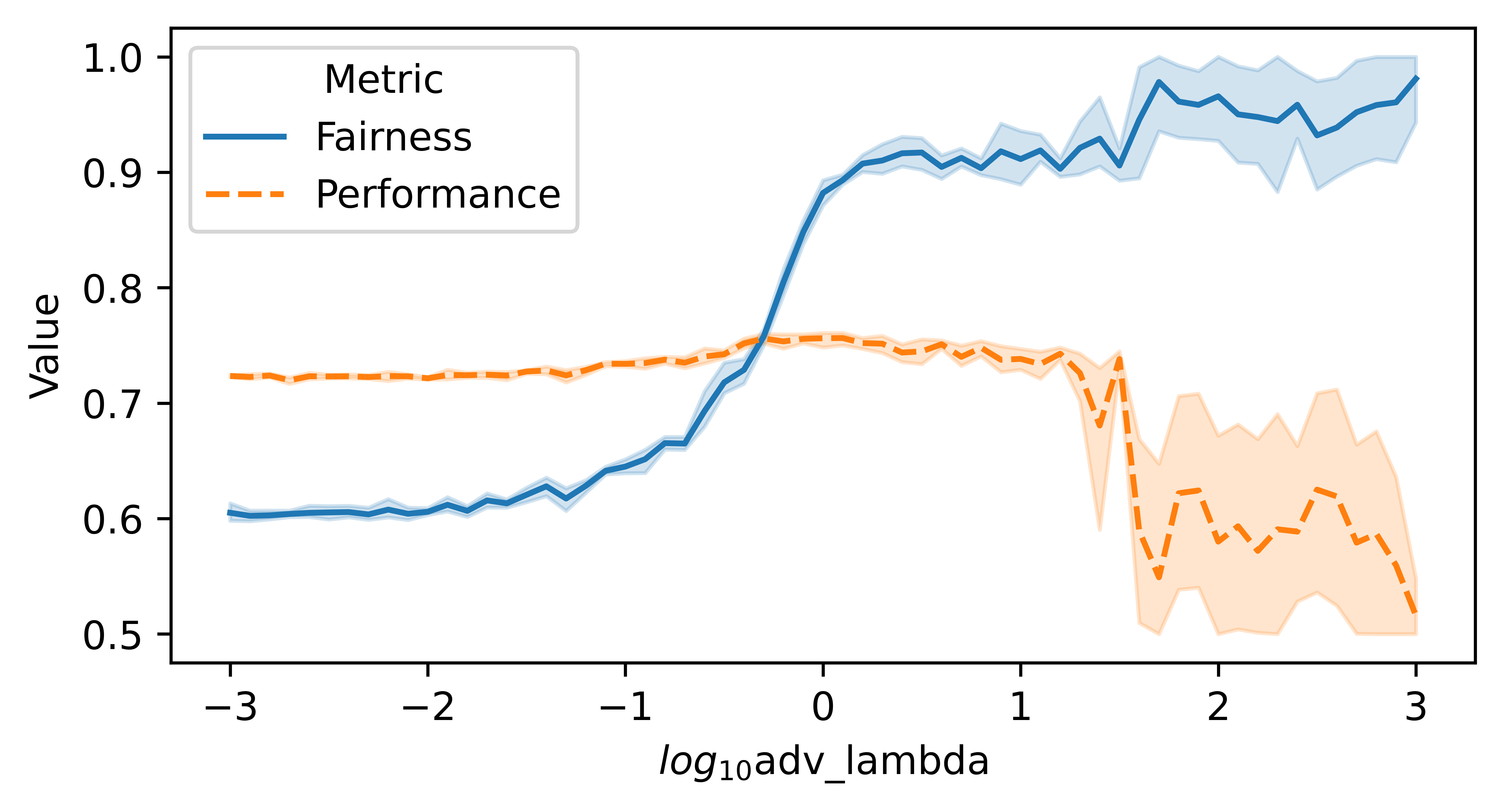
(a) Tuning Adv trade-off hyperparameter

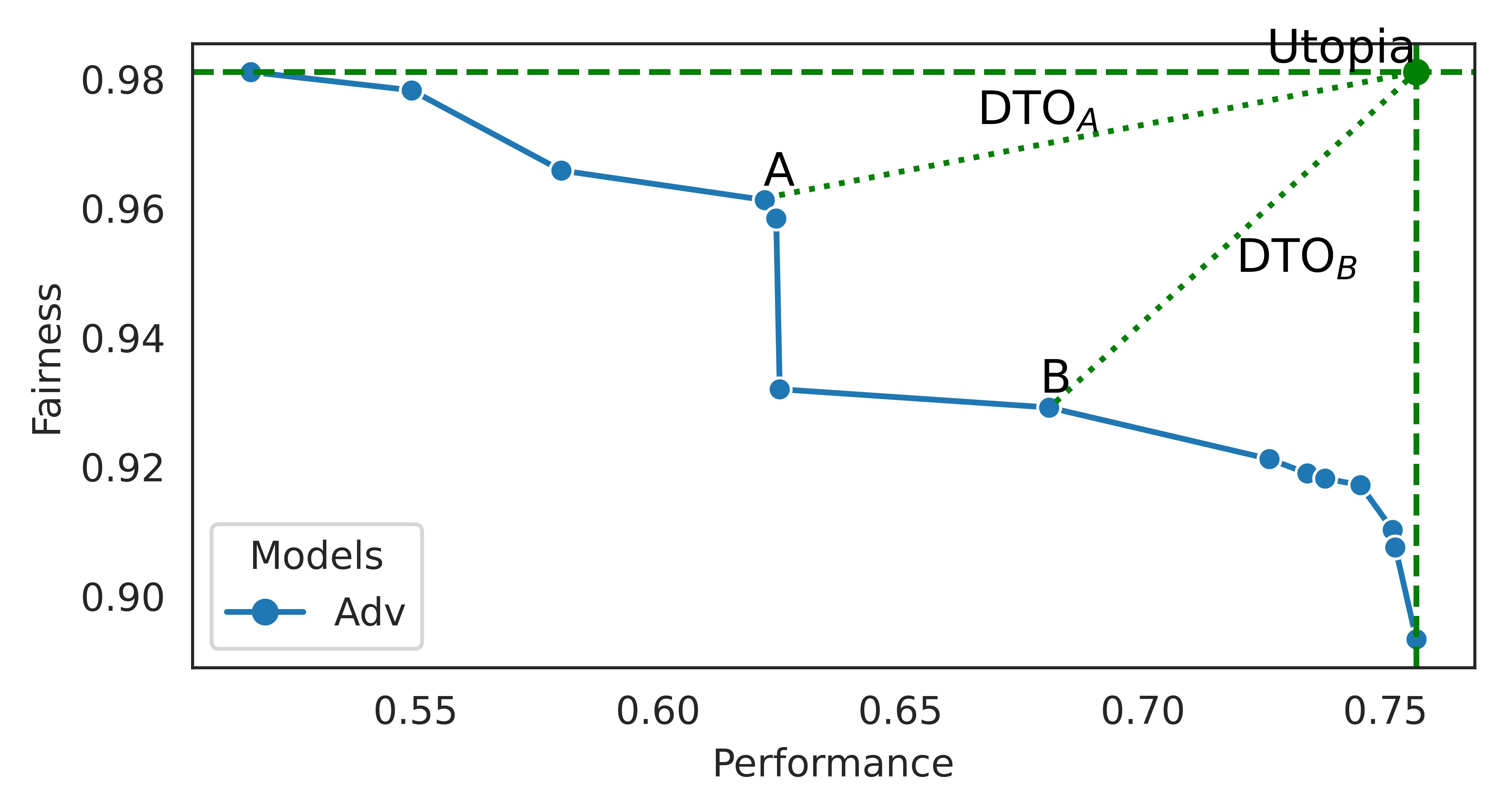
(b) Adv trade-off

Figure 2: An example of performance–fairness trade-off with respect to different values of the strength for the additional loss for discriminator unlearning in Adv. The shaded area refers to 95% CI. Figure 2(b) also provides an example for DTO. The green dashed vertical and horizontal lines denote the best performance and fairness, respectively, and their intersection point is the Utopia point. The length of the green dotted lines from A and B to the Utopia point are the DTO for candidate models A and B, respectively.

Typically, instead of looking at the performance/fairness for different trade-off hyperparameter values, it is more meaningful to focus on the Pareto plots (Figure 2(b)), which show the maximum fairness that can be achieved at different performance levels, and vice versa.

DTO is a metric to quantify the performance–fairness tradeoff, which measures the Distance To the Optimal point for candidate models (Salukvadze, 1971; Marler and Arora, 2004; Han et al., 2021a). Note that the DTO can not only be used to compare different methods, but also for early stopping and model selection. Figure 2(b) provides an example of model selection based on DTO, where the optimal (Utopia) point at the top-right corner and DTO scores are the normalized Euclidean distance (length of green dotted lines) between the optimal points and candidate models.

In this paper, we use DTO for early stopping and method comparison, while selecting the best model for each method based on the results of Standard.

3 Methods

(a) Standard Adversarial

(b) Augmented Adversarial

(c) Augmentation layer

Figure 3: Proposed model architectures. Dashed lines denote gradient reversal in adversarial learning. Green and blue rounded rectangles are the trainable neural network layers for target label classification and bias mitigation, resp. Red circles are operations.

Here we describe the methods employed in this paper. Formally, as shown in Figure 3(a), given an input $\mathbf{x}$ annotated with main task label $\mathbf{y}$ and protected attribute label $\mathbf{g}$, a main task model consists of two connected parts: the encoder $\mathbf{h}=m(\mathbf{x};\bm{\theta}^{m})$ is trained to compute the hidden representation from an input $\mathbf{x}$, and the classifier makes prediction, $\hat{\mathbf{y}}=f(\mathbf{h};\bm{\theta}^{f})$. During training, a discriminator $d$, parameterized by $\bm{\phi}^{d}$, is trained to predict $\hat{\mathbf{g}}=d(\mathbf{h};\bm{\phi}^{d})$ from the final hidden-layer representation $\mathbf{h}$. The discriminator is only used as a regularizer during training, and will be dropped at the test time, i.e., the final model with adversarial training is the same as a naively trained model at the inference time.

3.1 Adversarial Learning

Following the setup of Li et al. (2018a); Han et al. (2021c), the optimisation objective for standard adversarial training is:

$$\min_{\bm{\theta}^{m},\bm{\theta}^{f}}\max_{\bm{\phi}^{*}}\mathcal{X}(\mathbf{y},\hat{\mathbf{y}})-\lambda\mathcal{X}(\mathbf{g},\hat{\mathbf{g}})$$ (1)

where $\bm{\phi}^{*}=\{\bm{\phi}^{d}\}$, $\mathcal{X}$ is the cross entropy loss, and $\lambda$ is a trade-off hyperparameter. Solving this minimax optimization problem encourages the main task model hidden representation $\mathbf{h}$ to be informative to $f$ and to be uninformative to $d$.

3.2 Discriminator with Augmented Representation

As illustrated in Figure 3(b), we propose augmented discrimination, a novel means of strengthening the adversarial component. Specifically, an extra augmentation layer $a$ is added between $m$ and $d$, where $a$ takes the $\mathbf{y}$ into consideration to create richer features, i.e., $\hat{\mathbf{g}}=d(a(\mathbf{h};\mathbf{y};\bm{\phi}^{a});\bm{\phi}^{d})$.

Augmentation Layer

Figure 3(c) shows the architecture of the proposed augmentation layer. Inspired by the domain-conditional model of Li et al. (2018b), the augmentation layer $a$ consists of one shared projector and $|C|$ specific projectors,$\{m^{s},{m^{\prime}}_{1},{m^{\prime}}_{2},\dots,{m^{\prime}}_{|C|}\}$, where $|C|$ is the number of target classes.

Formally, let $m^{s}(\mathbf{h};\bm{\phi}^{s})$ be a function parameterized by $\bm{\phi}^{s}$ which projects a hidden representation $\mathbf{h}$ to $\mathbf{h}^{s}$ representing features w.r.t $\mathbf{g}$ that are shared across classes, and ${m^{\prime}}_{j}(\mathbf{h};\bm{\phi}^{j})$ be a class-specific function to the $j$-th class which projects the same hidden representation $\mathbf{h}$ to ${\mathbf{h}^{\prime}}^{j}$ capturing features that are private to the $j$-th class. In this paper, we employ the same architecture for shared and all private projectors. The resulting output of the augmentation layer is

$$\mathbf{h}^{a}=a(\mathbf{h};\mathbf{y};\bm{\phi}^{a})=\mathbf{h}^{s}+\sum_{j=1}^{|C|}\mathbf{y}_{i,j}{\mathbf{h}^{\prime}}^{j},$$

where $\bm{\phi}^{a}=\{\bm{\phi}^{s},\bm{\phi}^{1},\dots,\bm{\phi}^{|C|}\}$, and $\mathbf{y}_{i,\mathrel{\mathop{\ordinarycolon}}}$ is 1-hot. Moreover, let $\bm{\phi}^{*}=\{\bm{\phi}^{d},\bm{\phi}^{a}\}$, the training objective is the same as Equation 1.

Intuitively, $d$ is able to make better predictions over $\mathbf{g}$ based on $\mathbf{h}^{a}$ than the vanilla $\mathbf{h}$ due to the enhanced representations provided by $a$. More formally, as the augmented discriminator models the conditional probability $\Pr(g|h,y)$, the unlearning of the augmented discriminator encourages conditional independence $\mathbf{h}\perp\mathbf{g}|\mathbf{y}$, which corresponds directly to the equal opportunity criterion.

4 Experiments

In order to compare our method with previous work, we follow the experimental setting of Han et al. (2021c). We provide full experimental details in Appendix B.

4.1 Evaluation Metrics

Following Han et al. (2021c); Ravfogel et al. (2020), we use overall accuracy as the performance metric, and measure TPR GAP for equal opportunity fairness. For multiclass classification tasks, we report the quadratic mean (RMS) of TPR GAP over all classes. While in a binary classification setup, TPR and TNR are equivalent to the TPR of the positive and negative classes, respectively, so we employ the RMS TPR GAP in this case also. For GAP metrics, the smaller, the better, and a perfectly fair model will achieve 0 GAP. We further measure the fairness as 1-GAP, the larger, the better.

More specifically, the calculation of RMS TPR GAP consists of aggregations at the group and class levels. At the group level, we measure the absolute TPR difference of each class between each group and the overall TPR $GAP^{TPR}_{G,y}=\sum_{g\in{G}}|TPR_{g,y}-TPR_{y}|$, and at the next level, we further perform the RMS aggregation at the class level to get the RMS TPR GAP as $GAP=\sqrt{\frac{1}{|Y|}\sum_{y\in{Y}}(GAP^{TPR}_{G,y})^{2}}$.

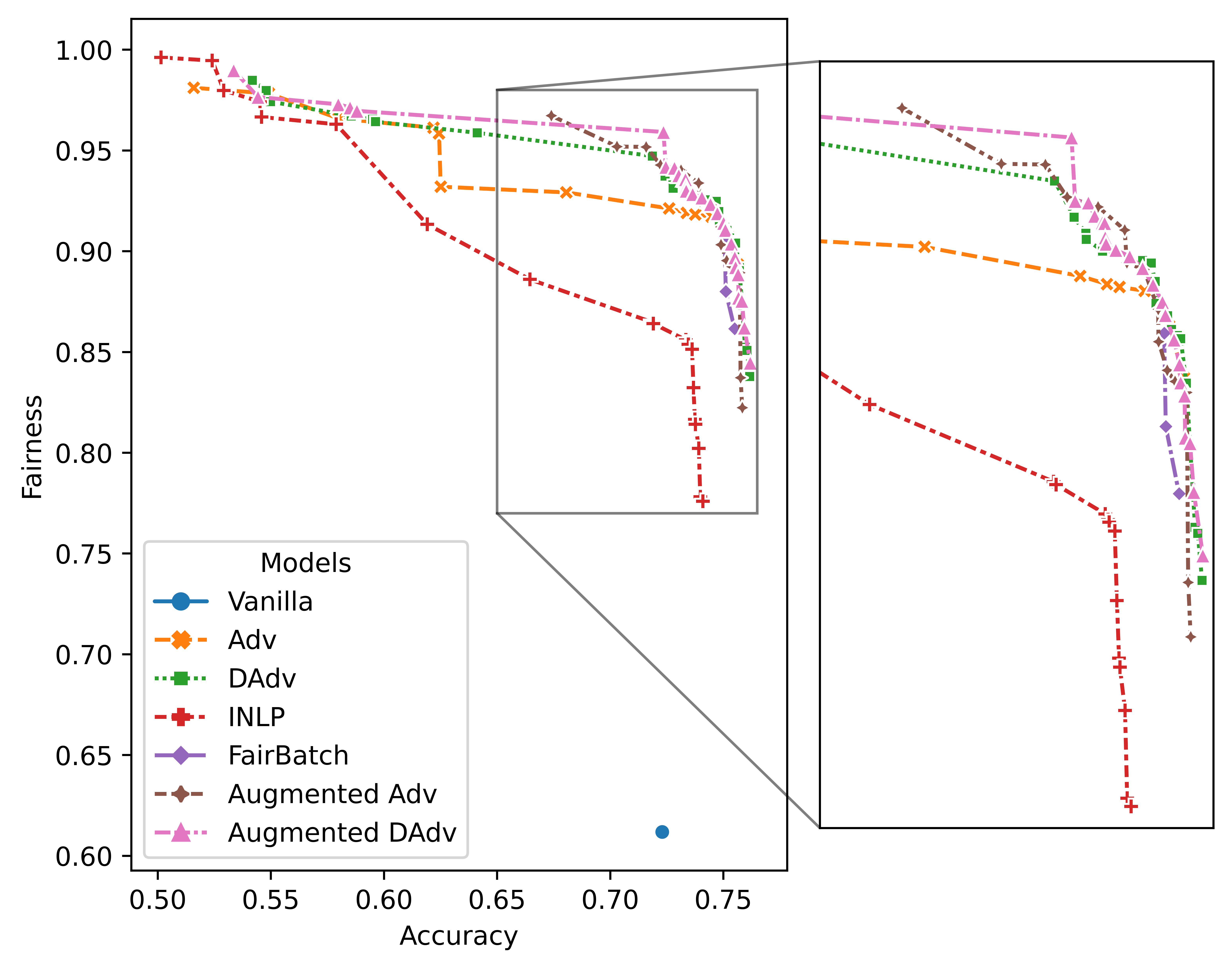
(a) Moji

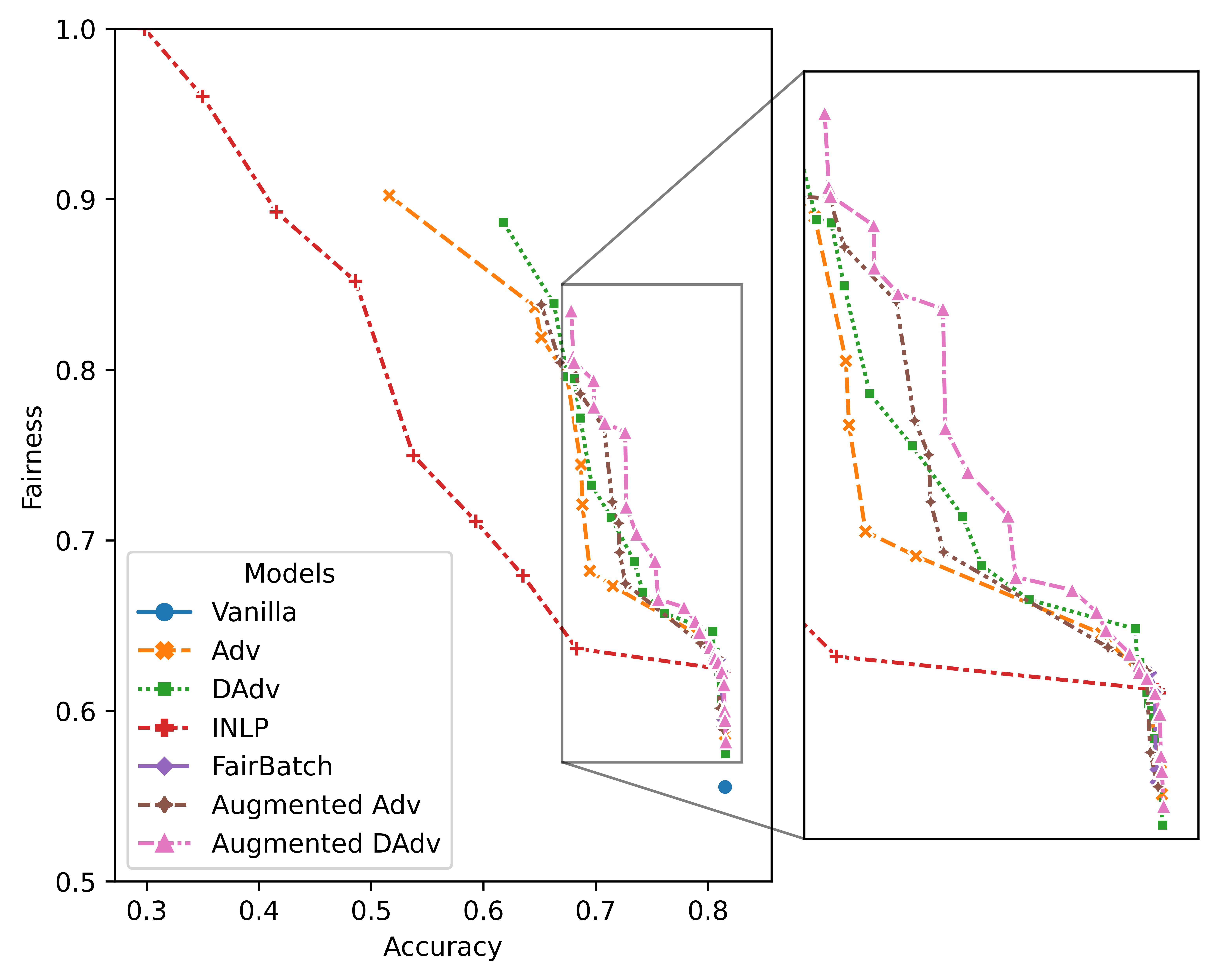
(b) Bios

Figure 4: Pareto frontiers of trade-offs between performance and fairness. The top-right represents ideal model with the idea performance and fairness.

4.2 Dataset

Following Subramanian et al. (2021), we conduct experiments over two NLP classification tasks — sentiment analysis and biography classification — using the same dataset splits as prior work.

Moji

This sentiment analysis dataset was collected by Blodgett et al. (2016), and contains tweets that are either African American English (AAE)-like or Standard American English (SAE)-like. Each tweet is annotated with a binary ‘race’ label (based on language use: either AAE or SAE) and a binary sentiment score determined by (redacted) emoji contained in it.

Bios

The second task is biography classification (De-Arteaga et al., 2019; Ravfogel et al., 2020), where biographies were scraped from the web, and annotated for the protected attribute of binary gender and target label of 28 profession classes.

Besides the binary gender attribute, we additionally consider economic status as a second protected attribute. Subramanian et al. (2021) semi-automatically label economic status (wealthy vs. rest) based on the country the individual is based in, as geotagged from the first sentence of the biography. For bias evaluation and mitigation, we consider the intersectional groups, i.e., the Cartesian product of the two protected attributes, leading to 4 intersectional classes: female–wealthy, female–rest, male–wealthy, and male–rest.

4.3 Models

We first implement a naively trained model on each dataset, without explicit debiasing. On the Moji dataset, we use DeepMoji (Felbo et al., 2017) as the fixed encoders to get 2304d representations of input texts. For the Bios dataset, we use uncased BERT-base (Devlin et al., 2019), taking the ‘AVG’ representations extracted from the pretrained model, without further fine-tuning.

For adversarial method, both the Adv and augmented Adv, we jointly train the discriminator and classifier. Again, we follow Han et al. (2021c) in using a non-linear discriminator, which is implemented as a trainable 3-layer MLP.

A common problem is that a large number of instances are not annotated with protected attributes, e.g. only 28% instances in the Bios dataset are annotated with both gender and economic status labels. The standard adversarial method has required all training instances are annotated with protected attributes, and thus can only be trained over a full-labelled subset, decreasing the training set size significantly. To maintain the performance of the debiased model, we follow Han et al. (2021b) in decoupling the training of the model and the discriminator, making it possible to use all instances for model training at a cost of the performance-fairness trade-off.

4.4 Main results

Figure 4 shows the results. Each point denotes a candidate model, and we take the average over 5 runs with different random seeds.

Trade-off 5% Trade-off 10% Model Accuracy$\uparrow$ Fairness$\uparrow$ DTO $\downarrow$ Accuracy$\uparrow$ Fairness$\uparrow$ DTO $\downarrow$ Standard $72.2981$ $\pm$ $00.4576$ $61.1870$ $\pm$ $01.4356$ $47.6849$ $72.2981$ $\pm$ $00.4576$ $61.1870$ $\pm$ $01.4356$ $47.6849$ Adv $68.0645$ $\pm$ $10.1305$ $92.9164$ $\pm$ $04.0835$ $32.7117$ $62.5106$ $\pm$ $11.5933$ $93.1983$ $\pm$ $06.2517$ $38.1014$ DAdv $71.8605$ $\pm$ $00.4752$ $94.7193$ $\pm$ $01.3539$ $28.6307$ $64.1210$ $\pm$ $12.8721$ $95.8738$ $\pm$ $03.7152$ $36.1155$ INLP 70.92 85.36 $32.5575$ 61.92 91.33 $39.0584$ FairBatch $74.1810$ $\pm$ $00.6203$ $90.4656$ $\pm$ $01.3971$ $27.5232$ $74.1810$ $\pm$ $00.6203$ $90.4656$ $\pm$ $01.3971$ $27.5232$ A-Adv $70.3001$ $\pm$ $00.4699$ $95.1914$ $\pm$ $01.1671$ $30.0867$ $67.3968$ $\pm$ $01.1729$ $96.7237$ $\pm$ $00.6380$ $32.7674$ A-DAdv $72.3556$ $\pm$ $00.9952$ $95.9129$ $\pm$ $01.5552$ $27.9449$ $64.2336$ $\pm$ $09.1795$ $95.7233$ $\pm$ $02.4305$ $36.0212$

(a) Moji

Trade-off 5% Trade-off 10% Model Accuracy$\uparrow$ Fairness$\uparrow$ DTO $\downarrow$ Accuracy$\uparrow$ Fairness$\uparrow$ DTO $\downarrow$ Standard $81.5181$ $\pm$ $0.2435$ $55.5411$ $\pm$ $2.9533$ $48.1475$ $81.5181$ $\pm$ $0.2435$ $55.5411$ $\pm$ $2.9533$ $48.1475$ Adv $77.2195$ $\pm$ $2.9662$ $61.9941$ $\pm$ $2.2156$ $44.3102$ $74.5883$ $\pm$ $2.5882$ $62.8701$ $\pm$ $2.8081$ $44.9932$ DAdv $78.0985$ $\pm$ $1.3802$ $62.5999$ $\pm$ $1.8781$ $43.3410$ $73.4351$ $\pm$ $3.7638$ $68.7555$ $\pm$ $4.9055$ $41.0111$ INLP 80.41 59.39 $45.0919$ 80.41 59.39 $45.0919$ FairBatch $80.5659$ $\pm$ $0.6283$ $61.7986$ $\pm$ $2.0357$ $42.8606$ $80.5659$ $\pm$ $0.6283$ $61.7986$ $\pm$ $2.0357$ $42.8606$ A-Adv $77.6374$ $\pm$ $2.3608$ $63.7065$ $\pm$ $2.5969$ $42.6298$ $73.7561$ $\pm$ $5.1941$ $66.4149$ $\pm$ $5.7328$ $42.6228$ A-DAdv $77.4654$ $\pm$ $1.6841$ $63.7290$ $\pm$ $3.4463$ $42.7012$ $73.0678$ $\pm$ $2.8756$ $71.6363$ $\pm$ $4.6660$ $39.1133$

(b) Bios

Table 1: Evaluation results $\pm$ standard deviation ($\%$) on the test set of sentiment analysis (Moji) and biography classification (Bios) tasks, averaged over 5 runs with different random seeds. DTO is measured by the normalized Euclidean distance between each model and the ideal model, and lower is better. Due to the fact that INLP is a Post-processing approach which cannot be run end to end, we only report the its results for 1 run. Least biased models within a given performance tradeoff thresholds are chosen from development set.

We compare our proposed augmented discriminator against the standard discriminator and various competitive baselines: (1) Standard, which only optimizes performance during training; (2) Adv (Li et al., 2018a), which adjusts the strength of adversarial training ($\lambda$); (3) DAdv (Han et al., 2021c), which is the SOTA Adv variation that removes protected information from different aspects, and both $\lambda$ and the strength of orthogonality constraints are tuned; (4) INLP (Ravfogel et al., 2020), which is a post-processing method, and we tune the number of iteration for null-space projections to control the trade-off, and (5) FairBatch (Roh et al., 2021), which is the STOA pre-processing method, and we tune adjustment rate for the outer optimization to achieve different trade-offs.

In terms of our own methods, we adopt the Augmentation layer (Figure 3(c) for both Adv and DAdv, resulting the Augmented Adv and Augmented DAdv, respectively. Except for the trade-off hyperparameters, other hyperparameters of each model are the same to Standard.

Over both datasets, augmented methods achieve better performance–fairness trade-off. I.e., the adversarial method with augmented discriminator achieves better fairness at the same accuracy level, and achieves better accuracy at the same fairness level. A-Adv, A-DAdv, and DAdv achieve similar results (their trade-off lines almost overlap), while these methods outperform Adv consistently.

Moreover, our proposed methods also achieved better trade-offs than other baseline methods: INLP achieves the worst trade-off over two datasets, as it is a post-process method and the model will not be updated during debiasing; and FairBatch can achieve a similar trade-off as our proposed methods, but its ability of debiasing is limited due to its resampling strategy.

Trade-off 5% Trade-off 10% Model Accuracy$\uparrow$ Fairness$\uparrow$ DTO $\downarrow$ Accuracy$\uparrow$ Fairness$\uparrow$ DTO $\downarrow$ Adv $68.0645$ $\pm$ $10.1305$ $92.9164$ $\pm$ $4.0835$ $32.7117$ $62.5106$ $\pm$ $11.5933$ $93.1983$ $\pm$ $06.2517$ $38.1014$ A-Adv $70.3001$ $\pm$ $0.4699$ $95.1914$ $\pm$ $1.1671$ $30.0867$ $67.3968$ $\pm$ $01.1729$ $96.7237$ $\pm$ $00.6380$ $32.7674$ Adv + Large $72.4706$ $\pm$ $02.2792$ $92.0152$ $\pm$ $3.1307$ $28.6640$ $72.4706$ $\pm$ $02.2792$ $92.0152$ $\pm$ $03.1307$ $28.6640$ A-Adv + BT $71.3853$ $\pm$ $04.1419$ $90.4159$ $\pm$ $5.4043$ $30.1770$ $66.1765$ $\pm$ $09.8215$ $93.4086$ $\pm$ $04.4786$ $34.4597$ Adv +$\mathbf{y}$ $67.8895$ $\pm$ $10.0691$ $93.7331$ $\pm$ $3.8867$ $32.7164$ $67.8895$ $\pm$ $10.0691$ $93.7331$ $\pm$ $03.8867$ $32.7164$ Adv + Sep $68.3046$ $\pm$ $10.3392$ $95.3054$ $\pm$ $3.2996$ $32.0412$ $63.7159$ $\pm$ $12.4834$ $96.2037$ $\pm$ $04.2051$ $36.4821$

(a) Moji

Trade-off 5% Trade-off 10% Model Accuracy$\uparrow$ Fairness$\uparrow$ DTO $\downarrow$ Accuracy$\uparrow$ Fairness$\uparrow$ DTO $\downarrow$ Adv $77.2195$ $\pm$ $2.9662$ $61.9941$ $\pm$ $2.2156$ $44.3102$ $74.5883$ $\pm$ $2.5882$ $62.8701$ $\pm$ $2.8081$ $44.9932$ A-Adv $77.6374$ $\pm$ $2.3608$ $63.7065$ $\pm$ $2.5969$ $42.6298$ $73.7561$ $\pm$ $5.1941$ $66.4149$ $\pm$ $5.7328$ $42.6228$ Adv + Large $77.8762$ $\pm$ $2.8663$ $62.0592$ $\pm$ $1.2736$ $43.9200$ $75.3829$ $\pm$ $5.3457$ $64.0187$ $\pm$ $4.9486$ $43.5965$ A-Adv + BT $77.3251$ $\pm$ $3.0600$ $63.0041$ $\pm$ $5.0249$ $43.3918$ $74.8598$ $\pm$ $5.1214$ $65.3661$ $\pm$ $6.8683$ $42.7965$ Adv + $\mathbf{y}$ $77.6439$ $\pm$ $1.0993$ $59.8756$ $\pm$ $2.6541$ $45.9322$ $71.9278$ $\pm$ $3.5615$ $64.1095$ $\pm$ $4.5137$ $45.5651$ Adv + Sep $77.5513$ $\pm$ $3.3442$ $65.4962$ $\pm$ $4.6331$ $41.1638$ $72.3909$ $\pm$ $4.8889$ $67.0381$ $\pm$ $6.8553$ $42.9970$

(b) Bios

Table 2: Evaluation results $\pm$ standard deviation ($\%$) on the test set of sentiment analysis (Moji) and biography classification (Bios) tasks, averaged over 5 runs with different random seeds. Least biased models within a given performance tradeoff thresholds are chosen from development set. Adv + Large trains larger discriminators with more parameters than A-Adv as discussed in Section 5.1. A-Adv + BT employs the instance reweighting for the A-Adv (Section 5.2). Adv +$\mathbf{y}$ and Adv + Sep are alternative ways of conditional unlearning as discussed in  Section 5.3 which takes class labels as inputs and trains class-specific discriminators, respectively.

Model Moji Bios Adv 181,202 181,202 A-Adv 542,402 5,057,402 Adv + Large 680,450 9,013,250

Table 3: Number of parameters of discriminators over Moji and Bios datasets.

4.5 Constrained analysis

As shown in Figure 4, Pareto curves of different models highly overlap with each other. They can even have multiple intersections, making it hard to say which model strictly outperforms the others. Alternatively, we follow Subramanian et al. (2021) in comparing the fairest models under a minimum performance constraint, where the fairest models that exceed a performance threshold on the development set are chosen, and evaluated on the test set. We provide results under two constrained scenarios — fairest models on the development set trading off 5% and 10% of accuracy.

Table 5(a) shows the results over Moji dataset. With a performance trade-off up to 5%, both A-Adv and A-DAdv are strictly better than their base models Adv and DAdv, respectively. Also, A-DAdv shows the best fairness than others and consistently outperforms A-Adv.

In terms of other baseline methods, INLP shows worse performance and fairness than others. While for FairBatch, although it shows the smallest DTO (i.e., best trade-off), its ability of bias mitigation is limited. In both settings, FairBatch can only achieve a 0.90 fairness score, while A-Adv and A-Adv can achieve a 0.95 fairness score.

For a slack of up to 10% performance trade-off, augmented adversarial models strictly outperform their base models. However, when focusing on the A-DAdv, it can be seen that given a 10% performance trade-off, the fairness score is even not as good as that at the 5% level. The less fairness is caused by the inconsistency between the results over the development set and test set, i.e., the fairest model is selected based on the development set but does not generalize well on the test set.

For the occupation classification, results are summarized in Table 5(b). Similarly, our proposed methods consistently outperform others for both 5% and 10% performance settings, confirming the conclusion based on trade-off plots that adding augmentation layers for adversarial debiasing leads to better fairness.

5 Analysis

To better understand the effectiveness of our proposed methods, we perform three sets of experiments: (1) analysis of the effects of extra parameters in the Augmentation layer, (2) an ablation study of the effect of balanced discriminator training, and (3) a comparison with alternative ways of incorporating target labels in adversarial training. Similar to constrained analysis, we report the fairest models under a minimum performance constraint in Table 2.

5.1 Affects of extra parameters

Augmentation layers increase the number of parameters in discriminators, and thus an important question is whether the gains of augmentation layers are because of additional parameters.

We conduct experiments with two scenarios by controlling the number of parameters of a discriminator in Adv, namely Adv + Large, and compare it with A-Adv models. Specifically, we employ a larger discriminator with an additional layer and more hidden units within each layer, leading to roughly the same number of parameters as the augmented discriminator.

Table 3 summaries the number of parameters of discriminators under different settings. For Adv, the discriminators are 2-layer MLP. Thus its parameter size is only affected by its architecture, resulting in the same amount for two datasets. While for A-Adv, the amount of class-specific components within the augmentation layer is determined by the total distinct target classes, which are 2 and 28 for Moji and Bios, respectively, leading to a much larger discriminator for the Bios dataset.

As shown in Table 2, although Adv + Large contains more parameters than others, it is not as good as A-Adv. Over the Moji dataset, Adv + Large achieves a better trade-off, however, the best fairness that can be achieved is limited to 0.92, which is similar to the FairBatch method. Similarly, for Bios (Table 6(b)), Adv + Large leads to less fair models, and worse trade-offs than A-Adv.

5.2 Balanced discriminator training

One problem is that the natural distribution of the demographic labels is imbalanced. E.g.  in Bios, 87% of nurses are female while 90% of surgeons are male. A common way of dealing with this label imbalance is instance reweighting (Han et al., 2021a), which reweights each instance inversely proportional to the frequency of its demographic label within its target class when training the discriminators.

We experiment with the balanced version of discriminator training to explore the impact of such balanced training methods. The instance weighting is only applied to the discriminator training, while during unlearning, instances are assigned identical weights to reflect the actual proportions of protected groups.

A-Adv methods with balanced training are denoted as A-Adv + BT, and corresponding results over two datasets are shown in Table 2. In contrast to our intuition that balanced training enhances the ability to identify protected attributes and leads to better bias mitigation, the A-Adv + BT methods can not improve the trade-offs in any setting. This might be because of the imbalanced training of the main task model, which mainly focuses on the majority group within each class, in which case the imbalanced trained discriminator is also able to identify protected information properly.

5.3 Alternative ways of conditional unlearning

Essentially, our method is one way of unlearning protected information conditioned on the class labels. Alternatively, we can concatenate the hidden representations $\mathbf{h}$ and target labels $\mathbf{y}$ as the inputs to the discriminator (Wadsworth et al., 2018), as well as train a set of discriminators, one for each target class (Zhao et al., 2019).

Taking target labels $\mathbf{y}$ as the inputs (Adv +$\mathbf{y}$) can only capture the target class conditions as a different basis, which is insufficient. As such, it can be seen from Table 2 that, Adv +$\mathbf{y}$ only leads to minimum improvements over the Adv, but is not as good as A-Adv.

The other alternative method, Adv + Sep which trains one discriminator for each target class, is the closed method to our proposed augmentation layers. However, Adv + Sep has two main limitations: (1) discriminators are trained separately, which cannot learn the shared information across different class like the shared component of augmentation layers, and (2) the training and unlearning process for multiple discriminators are much complicated, especially when combined with other variants of adversarial training, such as Ensemble Adv (Elazar and Goldberg, 2018) and DAdv (Han et al., 2021c) that employs multiple sub-discriminators.

As shown in Table 2, although Adv + Sep shows improvements to Adv +$\mathbf{y}$, A-Adv still outperforms Adv + Sep significantly (1 percentage point better in in terms of trade-off on average).

6 Conclusion

We introduce an augmented discriminator for adversarial debiasing. We conducted experiments over a binary tweet sentiment analysis with binary author race attribute and a multiclass biography classification with the multiclass protected attribute. Results showed that our proposed method, considering the target label, can more accurately identify protected information and thus achieves better performance–fairness trade-off than the standard adversarial training.

Ethical Considerations

This work aims to advance research on bias mitigation in NLP. Although our proposed method requires access to training datasets with protected attributes, this is the same data assumption made by adversarial training. Our target is to remove protected information during training better. To avoid harm and be trustworthy, we only use attributes that the user has self-identified for experiments. Moreover, once being trained, our proposed method can make fairer predictions without the requirement of demographic information. All data in this study is publicly available and used under strict ethical guidelines.

Appendix A Dataset

A.1 Moji

We use the train, dev, and test splits from Han et al. (2021c) of 100k/8k/8k instances, respectively. This training dataset has been artificially balanced according to demographic and task labels, but artificially skewed in terms of race–sentiment combinations, as follows: AAE–happy = 40%, SAE–happy = 10%, AAE–sad = 10%, and SAE–sad = 40%.

A.2 Bios

Since the data is not directly available, in order to construct the dataset, we use the scraping scripts of Ravfogel et al. (2020), leading to a dataset with 396k biographies. Following Ravfogel et al. (2020), we randomly split the dataset into train (65%), dev (10%), and test (25%).

Table 4 shows the target label distribution and protected attribute distribution.

Profession Total male_rest male_wealthy female_rest female_wealthy professor 21715 $0.091\,964$ $0.461\,708$ $0.072\,715$ $0.373\,613$ physician 7581 $0.084\,422$ $0.424\,482$ $0.079\,937$ $0.411\,159$ attorney 6011 $0.099\,152$ $0.511\,728$ $0.062\,219$ $0.326\,901$ photographer 4398 $0.110\,505$ $0.530\,923$ $0.055\,935$ $0.302\,638$ journalist 3676 $0.093\,308$ $0.407\,236$ $0.085\,691$ $0.413\,765$ nurse 3510 $0.011\,396$ $0.075\,499$ $0.149\,288$ $0.763\,818$ psychologist 3280 $0.064\,939$ $0.307\,012$ $0.105\,488$ $0.522\,561$ teacher 2946 $0.061\,439$ $0.351\,324$ $0.095\,044$ $0.492\,193$ dentist 2682 $0.113\,348$ $0.520\,880$ $0.063\,013$ $0.302\,759$ surgeon 2465 $0.123\,732$ $0.726\,572$ $0.023\,935$ $0.125\,761$ architect 1891 $0.116\,341$ $0.641\,460$ $0.034\,373$ $0.207\,827$ painter 1408 $0.088\,778$ $0.473\,011$ $0.075\,284$ $0.362\,926$ model 1362 $0.024\,963$ $0.149\,046$ $0.129\,956$ $0.696\,035$ poet 1295 $0.073\,359$ $0.459\,459$ $0.081\,853$ $0.385\,328$ software_engineer 1289 $0.137\,316$ $0.697\,440$ $0.024\,825$ $0.140\,419$ filmmaker 1225 $0.096\,327$ $0.555\,918$ $0.058\,776$ $0.288\,980$ composer 1045 $0.141\,627$ $0.704\,306$ $0.017\,225$ $0.136\,842$ accountant 1012 $0.094\,862$ $0.553\,360$ $0.063\,241$ $0.288\,538$ dietitian 730 $0.012\,329$ $0.050\,685$ $0.120\,548$ $0.816\,438$ comedian 499 $0.090\,180$ $0.693\,387$ $0.030\,060$ $0.186\,373$ chiropractor 474 $0.143\,460$ $0.618\,143$ $0.031\,646$ $0.206\,751$ pastor 453 $0.145\,695$ $0.593\,819$ $0.035\,320$ $0.225\,166$ paralegal 330 $0.027\,273$ $0.124\,242$ $0.148\,485$ $0.700\,000$ yoga_teacher 305 $0.029\,508$ $0.134\,426$ $0.121\,311$ $0.714\,754$ interior_designer 267 $0.041\,199$ $0.164\,794$ $0.123\,596$ $0.670\,412$ personal_trainer 264 $0.098\,485$ $0.412\,879$ $0.068\,182$ $0.420\,455$ dj 244 $0.155\,738$ $0.709\,016$ $0.024\,590$ $0.110\,656$ rapper 221 $0.153\,846$ $0.746\,606$ $0.009\,050$ $0.090\,498$ Total 72578 $0.088\,635\,67$ $0.450\,797\,76$ $0.074\,636\,94$ $0.385\,929\,62$

Table 4: Training set distribution of the Bios dataset.

Appendix B Reproducibility

B.1 Computing infrastructure

We conduct all our experiments on a Windows server with a 16-core CPU (AMD Ryzen Threadripper PRO 3955WX), two NVIDIA GeForce RTX 3090s with NVLink, and 256GB RAM.

B.2 Computational budget

Over the Moji dataset, we run experiments with 108 different hyperparameter combinations (each for 5 runs with different random seeds) in total, which takes around 300 GPU hours in total and 0.56 hrs for each run. Over the Bios dataset, we run experiments with 162 different hyperparameter combinations for around 466 GPU hours and 0.58 hrs for each run.

B.3 Model architecture and size

In this paper, we used pretrained models as fixed encoder, and the number of fixed parameters of DeepMoji (Felbo et al., 2017) for Moji and uncased BERT-base (Devlin et al., 2019) for Bios are approximately 22M and 110M, resp. The number of remaining trainable parameters of the main model is about 1M for both tasks.

As for the standard discriminator, we follow Han et al. (2021b) and use the same architecture for both tasks, leading to a 3-layer MLP classifier with around 144k parameters.

B.4 Hyperparameters

For each dataset, all main task model models in this paper share the same hyperparameters as the standard model. Hyperparameters are tuned using grid-search, in order to maximize accuracy for the standard model. Table 5 summaries search space and best assignments of key hyperparameters.

Best assignment Hyperparameter Search space Moji Bios number of epochs - 100 patience - 10 embedding size - 2304 768 hidden size - 300 number of hidden layers choice-integer[1, 3] 2 batch size loguniform-integer[64, 2048] 1024 512 output dropout uniform-float[0, 0.5] 0.5 0.3 optimizer - Adam (Kingma and Ba, 2015) learning rate loguniform-float[$10^{-6}$, $10^{-1}$] $3\times 10^{-3}$ $10^{-3}$ learning rate scheduler - reduce on plateau LRS patience - 2 epochs LRS reduction factor - 0.5

Table 5: Search space and best assignments.

To explore trade-offs of our proposed method at different levels, we tune $\lambda$ log-uniformly to get a series of candidate models. Specifically, the search space of $\lambda$ with respect to Moji and Bios are both loguniform-float[$10^{-3}$, $10^{3}$].

References

- Badjatiya et al. (2019) Pinkesh Badjatiya, Manish Gupta, and Vasudeva Varma. 2019. Stereotypical bias removal for hate speech detection task using knowledge-based generalizations. In The World Wide Web Conference, pages 49–59.
- Barocas et al. (2019) Solon Barocas, Moritz Hardt, and Arvind Narayanan. 2019. Fairness and Machine Learning. http://www.fairmlbook.org.
- Blodgett et al. (2016) Su Lin Blodgett, Lisa Green, and Brendan O’Connor. 2016. Demographic dialectal variation in social media: A case study of African-American English. In Proceedings of the 2016 Conference on Empirical Methods in Natural Language Processing, pages 1119–1130.
- Chouldechova (2017) Alexandra Chouldechova. 2017. Fair prediction with disparate impact: A study of bias in recidivism prediction instruments. Big data, 5(2):153–163.
- De-Arteaga et al. (2019) Maria De-Arteaga, Alexey Romanov, Hanna Wallach, Jennifer Chayes, Christian Borgs, Alexandra Chouldechova, Sahin Geyik, Krishnaram Kenthapadi, and Adam Tauman Kalai. 2019. Bias in bios: A case study of semantic representation bias in a high-stakes setting. In Proceedings of the Conference on Fairness, Accountability, and Transparency, pages 120–128.
- Devlin et al. (2019) Jacob Devlin, Ming-Wei Chang, Kenton Lee, and Kristina Toutanova. 2019. Bert: Pre-training of deep bidirectional transformers for language understanding. In Proceedings of the 2019 Conference of the North American Chapter of the Association for Computational Linguistics: Human Language Technologies, Volume 1 (Long and Short Papers), pages 4171–4186.
- Elazar and Goldberg (2018) Yanai Elazar and Yoav Goldberg. 2018. Adversarial removal of demographic attributes from text data. In Proceedings of the 2018 Conference on Empirical Methods in Natural Language Processing, pages 11–21.
- Felbo et al. (2017) Bjarke Felbo, Alan Mislove, Anders Søgaard, Iyad Rahwan, and Sune Lehmann. 2017. Using millions of emoji occurrences to learn any-domain representations for detecting sentiment, emotion and sarcasm. In Conference on Empirical Methods in Natural Language Processing (EMNLP).
- Feldman et al. (2015) Michael Feldman, Sorelle A Friedler, John Moeller, Carlos Scheidegger, and Suresh Venkatasubramanian. 2015. Certifying and removing disparate impact. In proceedings of the 21th ACM SIGKDD international conference on knowledge discovery and data mining, pages 259–268.
- Han et al. (2021a) Xudong Han, Timothy Baldwin, and Trevor Cohn. 2021a. Balancing out bias: Achieving fairness through training reweighting. arXiv preprint arXiv:2109.08253.
- Han et al. (2021b) Xudong Han, Timothy Baldwin, and Trevor Cohn. 2021b. Decoupling adversarial training for fair NLP. In Findings of the Association for Computational Linguistics: ACL-IJCNLP 2021, pages 471–477.
- Han et al. (2021c) Xudong Han, Timothy Baldwin, and Trevor Cohn. 2021c. Diverse adversaries for mitigating bias in training. In Proceedings of the 16th Conference of the European Chapter of the Association for Computational Linguistics: Main Volume, pages 2760–2765.
- Han et al. (2022) Xudong Han, Aili Shen, Yitong Li, Lea Frermann, Timothy Baldwin, and Trevor Cohn. 2022. fairlib: A unified framework for assessing and improving classification fairness. arXiv preprint arXiv:2205.01876.
- Hardt et al. (2016) Moritz Hardt, Eric Price, and Nati Srebro. 2016. Equality of opportunity in supervised learning. Advances in Neural Information Processing Systems, 29:3315–3323.
- Kingma and Ba (2015) Diederick P Kingma and Jimmy Ba. 2015. Adam: A method for stochastic optimization. In International Conference on Learning Representations (ICLR).
- Lahoti et al. (2020) Preethi Lahoti, Alex Beutel, Jilin Chen, Kang Lee, Flavien Prost, Nithum Thain, Xuezhi Wang, and Ed Chi. 2020. Fairness without demographics through adversarially reweighted learning. In Advances in Neural Information Processing Systems, volume 33, pages 728–740.
- Li et al. (2018a) Yitong Li, Timothy Baldwin, and Trevor Cohn. 2018a. Towards robust and privacy-preserving text representations. In Proceedings of the 56th Annual Meeting of the Association for Computational Linguistics (Volume 2: Short Papers), pages 25–30.
- Li et al. (2018b) Yitong Li, Timothy Baldwin, and Trevor Cohn. 2018b. What’s in a domain? learning domain-robust text representations using adversarial training. In Proceedings of the 2018 Conference of the North American Chapter of the Association for Computational Linguistics: Human Language Technologies, Volume 2 (Short Papers), pages 474–479, New Orleans, Louisiana. Association for Computational Linguistics.
- Marler and Arora (2004) R Timothy Marler and Jasbir S Arora. 2004. Survey of multi-objective optimization methods for engineering. Structural and multidisciplinary optimization, 26(6):369–395.
- Ravfogel et al. (2020) Shauli Ravfogel, Yanai Elazar, Hila Gonen, Michael Twiton, and Yoav Goldberg. 2020. Null it out: Guarding protected attributes by iterative nullspace projection. In Proceedings of the 58th Annual Meeting of the Association for Computational Linguistics, pages 7237–7256.
- Roh et al. (2021) Yuji Roh, Kangwook Lee, Steven Euijong Whang, and Changho Suh. 2021. Fairbatch: Batch selection for model fairness. In Proceedings of the 9th International Conference on Learning Representations.
- Salukvadze (1971) M Ye Salukvadze. 1971. Concerning optimization of vector functionals. i. programming of optimal trajectories. Avtomat. i Telemekh, 8:5–15.
- Subramanian et al. (2021) Shivashankar Subramanian, Xudong Han, Timothy Baldwin, Trevor Cohn, and Lea Frermann. 2021. Evaluating debiasing techniques for intersectional biases. In Proceedings of the 2021 Conference on Empirical Methods in Natural Language Processing, pages 2492–2498, Online and Punta Cana, Dominican Republic. Association for Computational Linguistics.
- Wadsworth et al. (2018) Christina Wadsworth, Francesca Vera, and Chris Piech. 2018. Achieving fairness through adversarial learning: an application to recidivism prediction. FAT/ML Workshop.
- Wang et al. (2019) Tianlu Wang, Jieyu Zhao, Mark Yatskar, Kai-Wei Chang, and Vicente Ordonez. 2019. Balanced datasets are not enough: Estimating and mitigating gender bias in deep image representations. In Proceedings of the IEEE International Conference on Computer Vision, pages 5310–5319.
- Zhang et al. (2018) Brian Hu Zhang, Blake Lemoine, and Margaret Mitchell. 2018. Mitigating unwanted biases with adversarial learning. In Proceedings of the 2018 AAAI/ACM Conference on AI, Ethics, and Society, pages 335–340.
- Zhao et al. (2019) Han Zhao, Amanda Coston, Tameem Adel, and Geoffrey J Gordon. 2019. Conditional learning of fair representations. In International Conference on Learning Representations.
- Zhao et al. (2018) Jieyu Zhao, Tianlu Wang, Mark Yatskar, Vicente Ordonez, and Kai-Wei Chang. 2018. Gender bias in coreference resolution: Evaluation and debiasing methods. In Proceedings of the 2018 Conference of the North American Chapter of the Association for Computational Linguistics: Human Language Technologies, Volume 2 (Short Papers), pages 15–20.