Thermal entanglement and quantum coherence of a single electron in a double quantum dot with Rashba interaction

Abstract

In this work, we study the thermal quantum coherence and fidelity in a semiconductor double quantum dot. The device consists of a single electron in a double quantum dot with Rashba spin-orbit coupling in the presence of an external magnetic field. In our scenario, the thermal entanglement of the single electron is driven by the charge and spin qubits, the latter controlled by Rashba coupling. Analytical expressions are obtained for thermal concurrence and correlated coherence using the density matrix formalism. The main goal of this work is to provide a good understanding of the effects of temperature and several parameters in quantum coherence. In addition, our findings show that we can use the Rashba coupling to tune in the thermal entanglement, quantum coherence, as well as, the thermal fidelity behavior of the system. Moreover, we focus on the role played by thermal entanglement and correlated coherence responsible for quantum correlations. We observe that the correlated coherence is more robust than the thermal entanglement in all cases, so quantum algorithms based only on correlated coherence may be stronger than those based on entanglement.

I introduction

The quantum resources theories have been identified as an important field of research over the past few years chi ; stre1 . In particular, quantum coherence and quantum entanglement represent two fundamental features of non-classical systems that can each be characterized within an operational resource theory for quantum technological applications in the context of quantum information process benn-1 ; Ben2 ; lamico and emerging fields such as quantum metrology fro ; gio , quantum thermodynamics brandao ; lan and quantum biology lambert . Furthermore, over the past decade, the manipulation and generation of quantum correlations, has been widely investigated on various quantum systems such as Heisenberg models arne ; kam ; ro ; ro-1 , trapped ions tur , cavity quantum electrodynamics rai ; davi and so on.

One of the most promising physical systems for implementing quantum technologies, particularly quantum computing, is solid-state quantum dots (QDs) peta ; shin . There are proposals for QDs devices using either charge gor or spin benito ; loss ; an like qubits, or even both simultaneously jo ; yang . These quantum systems are of great interest because of their easy integration with existing electronics and scalability advantage ita ; urda . Moreover, in sanz ; sza , the quantum dynamics and the entanglement of two electrons inside the coupled double quantum dots were addressed, while in fan ; qin ; borge ; sou aspects related to the quantum correlations and the decoherence were investigated. Furthermore, several other properties have been investigated: quantum teleportation based on the double quantum dots choo , the quantum noise due to phonons induce steady-state in a double quantum dot charge qubit gia , multielectron quantum dots rao and thermal quantum correlations in two coupled double semiconductor charge qubits moi were also reported. More recently, a conceptual design of quantum heat machines has been developed using two coupled double quantum-dot systems as a working substance moi-1 .

In recent years, the spin-orbit interaction (SOI) in quantum dots has attracted much attention both theoretically and experimentally due to its potential roles in the quantum coherent manipulation of a spin qubit and spintronics fron ; hen . There are two different types of SOI in a semiconductor material, i.e., The Rashba SOI due to structural inversion asymmetry ras and Dresselhauss SOI due to the bulk inversion asymmetry dress .

Interest in the SOI process has been increased in recent past years as a set of potential applications of the SOI process was recently reported. For example, the spin-orbit-coupled quantum memory of a double quantum dot was investigated in chot . Recently, Yi-Chao Li et al. reported the influence of Rashba coupling in qubit gates with simultaneous transport in double quantum dots yili , and the transport of the spin shuttling between neighboring QDs is affected by the spin-orbit interaction ginzel .

On the other hand, quantum coherence arising from quantum superposition is a fundamental feature of quantum mechanics, and it has been widely recognized as the essence of bipartite and multipartite quantum correlations. The framework for quantifying coherence is based on taking into account an incoherent basis and defining an incoherent state as one which is diagonal on that basis. Several measurements have been proposed, and their properties have been investigated in detail over the years(see baum ; Hu ; stre2 , for instance). More recently, a new measure called correlated coherence tan ; tri has been introduced to investigate the relationship between quantum coherence and quantum correlations. Quantum correlated coherence is a measure of coherence with removed local parts; that is, all system coherence is stored entirely in quantum correlations.

Fast reliable spin manipulation in quantum dots is one of the most important challenges in spintronics and semiconductor-based quantum information. However, in real systems and with potential application to quantum information processing, it is crucial to understand the thermal robustness of quantum correlations at high temperatures, which is one of the main goals of this paper.

In this work, we aim to investigate the role of thermal entanglement and the quantum correlated coherence in a single electron spin in a double quantum dot in the presence of an external magnetic field. This electron contributes to tunneling, coupling the QDs and spin-flip tunneling caused by a Rashba spin-orbit coupling. We assume that the system is isolated from its respective electronic reservoirs, which remain in the strong Coulomb blockade regime, where one electron is permitted in a double quantum dot. We obtained analytical solutions, which allowed us to explore in detail the concurrence at zero temperature as well as the performance of the thermal entanglement; it is also possible to study the thermal evolution of the populations and thermal fidelity of the model. We also derived an analytical expression for the quantum correlated coherence and the difference between concurrence and quantum correlated coherence are investigated. In addition, it is compared the thermal entanglement with a quantum correlated coherence. Last but not least, the framework provided by the correlated coherence allows us to retrieve the same concepts of quantum discord and quantum entanglement, providing a unified view of these correlations, where the quantum discord is a measure of the quantum correlations going beyond entanglement ollivier ; wer . Note that, for a multipartite system, if the coherence of the global state is a resource that cannot be increased, the cost of creating discord can be expressed in terms of coherence yue ; ma . In this paper, we study these quantifiers in a thermal bath. The processing of quantum information can be done by controlling the temperature and the Rashba effect parameter present in the double quantum dot.

The outline of this paper is as follows. Section II defines the physical model and the method to treat it. Section III, briefly describes the definition of the concurrence ($\mathcal{C}$) and the correlated coherence ($\mathcal{C}_{cc}$). Thus the analytical expressions for them are found. In Section IV, we discuss some of the most interesting results like entanglement, populations, and correlated coherence taking into the account, the temperature effects, Rashba coupling and the tunneling parameter. Finally, in Section V, we present our conclusions.

II The model

The setup under investigation, depicted in Fig. 1, is a silicon device that consists of a double quantum dot is filled with a single electron and has two charge configurations, with the electron located either on the left ($L$) or right ($R$) dot, corresponding to position states labeled by $\left|L\right>$ and $\left|R\right>$ respectively. The Hamiltonian of the double quantum dot yili is given by

$$\begin{array}[]{ccc}H&=&\frac{\Delta}{2}(\mathbb{I}\otimes\sigma_{z})+t(\tau_{x}\otimes\mathbb{I})-\alpha(\tau_{y}\otimes\sigma_{x}),\end{array}$$ (1)

where $\tau_{x,y}$ are the Pauli matrices in the $\{\left|L\right>,\left|R\right>\}$ basis and $\sigma_{x,z}$ are the Pauli matrices describing the single electronic spin states $\{\left|0\right>,\left|1\right>\}$, $\mathbb{I}$ is the $2\times 2$ identity matrix. Here $\Delta$ is the Zeeman splitting generated by a constant external magnetic field along the $z$-axis, $t$ is the strength of the tunneling coupling between the two quantum dots, while the $\alpha$ is the spin-flip tunnel coupling due to the Rashba SOI ras contribution.

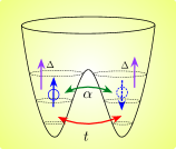
Figure 1: Schematic representation of the double quantum dot, the physical model includes the Rashba interaction $\alpha$. The spin of an electron is represented by the small sphere delocalized between two quantum dots.

The four eigenvectors of Hamiltonian (1) in the natural basis $\left\{\left|L0\right>,\left|L1\right>,\left|R0\right>,\left|R1\right>\right\}$ are

$$\left|\varphi_{1}\right> = A_{+}\left[ia_{+}\left(\left|L0\right>+\left|R0\right>\right)-\left|L1\right>+\left|R1\right>\right],$$

$$\left|\varphi_{2}\right> = A_{-}\left[ia_{-}\left(\left|L0\right>+\left|R0\right>\right)-\left|L1\right>+\left|R1\right>\right],$$

$$\left|\varphi_{3}\right> = B_{+}\left[ib_{+}\left(\left|L0\right>-\left|R0\right>\right)+\left|L1\right>+\left|R1\right>\right],$$

$$\left|\varphi_{4}\right> = B_{-}\left[ib_{-}\left(\left|L0\right>-\left|R0\right>\right)+\left|L1\right>+\left|R1\right>\right],$$ (2)

where $A_{\pm}=\frac{1}{\sqrt{2}\sqrt{a_{\pm}^{2}+1}}$, $a_{\pm}=\frac{\Omega_{+}\pm\sqrt{\Omega_{+}^{2}+4\alpha^{2}}}{2\alpha}$, $B_{\pm}=\frac{1}{\sqrt{2}\sqrt{b_{\pm}^{2}+1}}$, $b_{\pm}=\frac{\Omega_{-}\pm\sqrt{\Omega_{-}^{2}+4\alpha^{2}}}{2\alpha}$, $\Omega_{\pm}=\Delta\pm 2t$ and the corresponding eigenvalues are

$$\varepsilon_{1,2} = \pm\frac{1}{2}\sqrt{\Omega_{+}^{2}+4\alpha^{2}},$$ (3)

$$\varepsilon_{3,4} = \pm\frac{1}{2}\sqrt{\Omega_{-}^{2}+4\alpha^{2}}.$$ (4)

The system state in the thermal equilibrium is described by $\rho(T)=\frac{\exp(-\beta H)}{Z}$, where $\beta=1/k_{B}T$, with $k_{B}$ being the Boltzmann’s constant, $T$ is the absolute temperature and the partition function of the system is defined by $Z=Tr\left[\exp(-\beta H)\right]$.

II.1 The density operator

At thermal equilibrium, the double quantum dot density operator $\rho$ is described as

$$\rho_{AB}(T)=\left[\begin{array}[]{cccc}\rho_{11}&\rho_{12}&\rho_{13}&\rho_{14}\\ \rho_{12}^{*}&\rho_{22}&\rho_{14}&\rho_{24}\\ \rho_{13}&\rho_{14}^{*}&\rho_{11}&-\rho_{12}\\ \rho_{14}^{*}&\rho_{24}&-\rho_{12}^{*}&\rho_{22}\end{array}\right].$$ (5)

The elements of this density matrix, after a cumbersome algebraic manipulation, are given by

$$\begin{array}[]{ccl}\rho_{11}&=&\frac{A_{+}^{2}a_{+}^{2}e^{-\beta\varepsilon_{1}}+A_{-}^{2}a_{-}^{2}e^{-\beta\varepsilon_{2}}+B_{+}^{2}b_{+}^{2}e^{-\beta\varepsilon_{3}}+B_{-}^{2}b_{-}^{2}e^{-\beta\varepsilon_{4}}}{Z},\\ \rho_{12}&=&\frac{i[-A_{+}^{2}a_{+}e^{-\beta\varepsilon_{1}}-A_{-}^{2}a_{-}e^{-\beta\varepsilon_{2}}+B_{+}^{2}b_{+}e^{-\beta\varepsilon_{3}}+B_{-}^{2}b_{-}e^{-\beta\varepsilon_{4}}]}{Z},\\ \rho_{13}&=&\frac{A_{+}^{2}a_{+}^{2}e^{-\beta\varepsilon_{1}}+A_{-}^{2}a_{-}^{2}e^{-\beta\varepsilon_{2}}-B_{+}^{2}b_{+}^{2}e^{-\beta\varepsilon_{3}}-B_{-}^{2}b_{-}^{2}e^{-\beta\varepsilon_{4}}}{Z},\\ \rho_{14}&=&\frac{i[A_{+}^{2}a_{+}e^{-\beta\varepsilon_{1}}+A_{-}^{2}a_{-}e^{-\beta\varepsilon_{2}}+B_{+}^{2}b_{+}e^{-\beta\varepsilon_{3}}+B_{-}^{2}b_{-}e^{-\beta\varepsilon_{4}}]}{Z},\\ \rho_{22}&=&\frac{A_{+}^{2}e^{-\beta\varepsilon_{1}}+A_{-}^{2}e^{-\beta\varepsilon_{2}}+B_{+}^{2}e^{-\beta\varepsilon_{3}}+B_{-}^{2}e^{-\beta\varepsilon_{4}}}{Z},\\ \rho_{24}&=&\frac{-A_{+}^{2}e^{-\beta\varepsilon_{1}}-A_{-}^{2}e^{-\beta\varepsilon_{2}}+B_{+}^{2}e^{-\beta\varepsilon_{3}}+B_{-}^{2}e^{-\beta\varepsilon_{4}}}{Z},\end{array}$$

where $Z=\underset{i}{\sum}e^{-\beta\varepsilon_{i}}$.

Since $\rho_{AB}(T)$ represents a thermal state in equilibrium, the corresponding entanglement is then called thermal entanglement. In this paper, we consider a single electron spin in a double quantum dot with Rashba interaction. We found that, the charge qubit controlled by the interdot tunneling and the spin qubit driven by the Rashba interaction are responsible for the thermal entanglement of the model.

III Quantum Correlations

In this section we give a brief review concerning the definition and properties of the thermal entanglement and quantum coherence.

III.1 Thermal entanglement

In order to quantify the amount of entanglement associated with a given two-qubit state $\rho$, we consider concurrence $\mathcal{C}$ defined by Wootters wootters ; woo

$$\mathcal{C}={\rm{max}\left\{0,2max\left(\sqrt{\lambda_{i}}\right)-\sum_{i}\sqrt{\lambda_{i}}\right\},}$$ (6)

here $\lambda_{i}\>(i=1,2,3,4)$ are the eigenvalues in descending order of the matrix

$$R=\rho\left(\sigma^{y}\otimes\sigma^{y}\right)\rho^{\ast}\left(\sigma^{y}\otimes\sigma^{y}\right),$$ (7)

with $\sigma^{y}$ being the Pauli matrix. After straightforward calculations, the eigenvalues of the matrix $R$ can be expressed as

$$\lambda_{1} = \Theta+G+\sqrt{\Xi_{+}\Sigma_{+}},$$

$$\lambda_{2} = \Theta+G-\sqrt{\Xi_{+}\Sigma_{+}},$$

$$\lambda_{3} = \Theta-G+\sqrt{\Xi_{-}\Sigma_{-}},$$

$$\lambda_{4} = \Theta-G-\sqrt{\Xi_{-}\Sigma_{-}},$$ (8)

where

$$\begin{array}[]{ccl}G&=&-2\rho_{14}\rho_{12}+\rho_{11}\rho_{24}-\rho_{13}\rho_{22},\\ \Theta&=&\rho_{11}\rho_{22}-\rho_{13}\rho_{24}+|\rho_{14}|^{2}+|\rho_{12}|^{2},\\ \Xi_{\pm}&=&2\left(\rho_{12}\pm\rho_{14}\right)\left(\rho_{22}\pm\rho_{24}\right),\\ \Sigma_{\pm}&=&2\left(\rho_{13}\mp\rho_{11}\right)\left(\rho_{14}\pm\rho_{12}\right).\end{array}$$

Thus, the concurrence of this system can be written as cao

$$\mathcal{C}={\rm{max}\left\{0,\mid\sqrt{\lambda_{1}}-\sqrt{\lambda_{3}}\mid-\sqrt{\lambda_{2}}-\sqrt{\lambda_{4}}\right\},}$$ (9)

In this case, the analytical expression for the thermal concurrence is too large to be explicitly provided here, but it easy to recover following the above steps.

III.2 Correlated Coherence

Quantum coherence is an important feature in quantum physics and is of practical significance in quantum information processing task. Quantum coherence in a bipartite system can be contained both locally and in the correlations among the subsystems. The difference between the amount of coherence contained in the global state and the coherences that are purely local, is called correlated coherence, $\mathcal{C}_{cc}$ tan . For a bipartite quantum system, it becomes

$$\mathcal{C}_{cc}(\rho_{AB})=\mathcal{C}_{l_{1}}(\rho_{AB})-\mathcal{C}_{l_{1}}(\rho_{A})-\mathcal{C}_{l_{1}}(\rho_{B}),$$ (10)

where $\rho_{A}=Tr_{B}(\rho_{AB})$ and $\rho_{B}=Tr_{A}(\rho_{AB})$. Here, $A$ and $B$ stand for local subsystems.

In accordance with the set of properties that any appropriate measure of coherence should satisfy baum , a number of coherence measures have been put forward. Here we are concerned with the $l_{1}$-norm, it is a bona fide measure of coherence. The definition of the $l_{1}$-norm of coherence $\mathcal{C}_{l_{1}}$ is

$$\mathcal{C}_{l_{1}}(\rho)=\sum_{i\neq j}|\langle i|\rho|j\rangle|.$$ (11)

Quantum coherence is a basis-dependent concept, but we can choose an incoherent one for the local coherence, which will allow us to diagonalize $\rho_{A}$ and $\rho_{B}$. From Eq.(5), the reduced density matrix $\rho_{A}(T)$ will be given by

$$\rho_{A}(T)=\left(\begin{array}[]{cc}\rho_{11}+\rho_{22}&\rho_{13}+\rho_{24}\\ \rho_{13}+\rho_{24}&\rho_{11}+\rho_{22}\end{array}\right).$$ (12)

In a similar way, we obtain

$$\rho_{B}(T)=\left(\begin{array}[]{cc}2\rho_{11}&0\\ 0&2\rho_{22}\end{array}\right).$$ (13)

In order to analyze the correlated coherence, we perform a unitary transformation in the reduced density matrix $\rho_{A}(T)$. Thus, the unitary matrix results in

$$U=\left(\begin{array}[]{cc}\cos\theta&-e^{i\varphi}\sin\theta\\ e^{-i\varphi}\sin\theta&\cos\theta\end{array}\right).$$ (14)

So, let us have $\widetilde{\rho}_{A}(T)=U\,\rho_{A}(T)\,U^{\dagger}$. For $\rho_{B}(T)$ it is not necessary to perform any transformation, the operator $\rho_{B}(T)$ is already incoherent. On the other hand, the unitary transformation of the bipartite quantum state $\rho_{AB}(T)$ is given by $\widetilde{\rho}_{AB}(T)=\widetilde{U}\,\rho_{AB}(T)\,\widetilde{U}^{\dagger}$, where $\widetilde{U}=U\otimes\mathbb{I}$.

The unitary transformation will show the relationship between the global coherence and the local coherence for several choices of $\theta$ and $\varphi$ parameters. In particular, by setting $(\theta=\frac{\pi}{4},\varphi=0)$ in the Eq.(14), we obtain a matrix that diagonalize $\rho_{A}(T)$. This step provide us the basis set, where $A$ is locally incoherent. Thus, by inserting Eq.(14) into the Eq.(10), fixing $\theta=\frac{\pi}{4}$ and $\varphi=0$, we obtain an explicit expression for correlated coherence, that is,

$$\mathcal{C}_{cc}(\rho_{AB}(T))=|\rho_{14}+\rho_{12}|+|\rho_{14}+\rho_{12}^{*}|+|\rho_{12}-\rho_{14}|+|\rho_{12}^{*}-\rho_{14}|.$$ (15)

III.3 Fidelity of thermal state

The mixed-state fidelity can be defined as jo ; zhou

$$F(\rho_{1},\rho_{2})=Tr\sqrt{\rho_{2}^{1/2}\rho_{1}\rho_{2}^{1/2}}.$$ (16)

This quantity measures the degree of distinguishability between the two quantum states $\rho_{1}$ and $\rho_{2}$. Conversely, the quantum fidelity between the input pure state and the output mixed state is defined by

$$F=\langle\psi|\rho\left|\psi\right>,$$ (17)

where $\left|\psi\right>$ is the pure state and $\rho$ is the density operator state. This measurement provides the information of the overlap between the pure state $|\psi\rangle$ and the mixed state $\rho$. In the our case, we will study the thermal fidelity between the ground state $\left|\varphi_{2}\right>$ and the state of the system at temperature $T$. After some algebra, one finds

$$F(T)=\frac{\left[a_{+}^{2}(\rho_{11}+\rho_{13})+(\rho_{22}-\rho_{24})+2ia_{+}(\rho_{12}-\rho_{14}\right]}{\left[a_{+}^{2}+1\right]}.$$ (18)

Although this work is theoretical, a possible implementation of the device of a single electron in a double quantum dot with Rashba interaction is to consider the introduction of micromagnets in the device for spin-orbit interaction (SOI), see bor ; holl .

IV Results and Discussions

In this section, it is discussed the main results obtained in the foregoing section.

IV.1 Concurrence at zero temperature

Firstly, we investigate the influence of the tunneling coefficient $t$ and Rashba coupling $\alpha$ on the energy levels in zero temperature. The energy levels versus Zeeman splitting $\Delta$ is plotted in Fig. 2. Initially, we show in the same graph the two energies, each two-fold degenerate, for $t=0$ and $\alpha=0$ as indicated by dashed lines, red ($\varepsilon_{1}=\varepsilon_{3}$) and blue ($\varepsilon_{2}=\varepsilon_{4}$), respectively. On the other hand, for the solid curves, the tunneling between quantum dots ($t=2$) breaks the degeneracy at $\Delta=0$. Meanwhile, the Rashba coupling ($\alpha=0.1$) induces two anti-crossing points. In $\Delta=4$ for energy levels $\varepsilon_{3}$, and $\varepsilon_{4}$, and in $\Delta=-4$ for energy levels $\varepsilon_{1}$ and $\varepsilon_{2}$ From the above analysis, it is easy see that there is a strong correlation between interdot tunneling rates and degeneracy breaking of the eigenstates. As well as, one clear signature of the spin-orbit interaction is the formation of anti-crossing points in the electron energy spectrum.

In Fig. 3 we plot the concurrence $\mathcal{C}$ versus Rashba coupling $\alpha$, at zero temperature for fixed $t=0.1$ (solid curves), and $t=2$ (dashed curves), assuming several values of the $\Delta$. For tunneling parameter $t=0.1$, we observe a vigorous increase of the concurrence until reaching $\mathcal{C}\approx 0.9993$ for weak Zeeman splitting $\Delta=0.5$ and

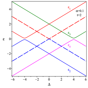
Figure 2: Spectrum energy of the DQD Hamiltonian $H$ as a function of $\Delta$, for fixed $t=2$ and $\alpha=0.1$ (solid curves). The dashed blue line and dashed red line show the energy levels for $t=0$ and $\alpha=0$.

Rashba coupling $\alpha=10$, in this case a single non-zero eigenvector that contributes to the entanglement is $\left|\varphi_{2}\right>\approx-0.491i\left(\left|L0\right>+\left|R0\right>\right)+0.508\left(-\left|L1\right>+\left|R1\right>\right)$, whereas when we consider $\alpha\rightarrow\infty$, the ground state reduces to $\left|\varphi_{2}\right>=-0.5i\left(\left|L0\right>+\left|R0\right>\right)+0.5\left(-\left|L1\right>+\left|R1\right>\right)$ and achieving maximum concurrence $(\mathcal{C}=1)$. Moreover, the curves show that the entanglement between the spin-charge qubits is smaller as the Zeeman splitting increases. From the same figure, we can see that as soon as the tunneling parameter increase say $t=2$, the concurrence is weaker than for weak tunneling regime (see dashed curves). Furthermore, still in same figure, it is observed that the concurrence is null at $\alpha=0$ for each parameter $t$ and $\Delta$ considered. Here the unentangled ground state is given by $\left|\varphi_{2}\right>=\frac{1}{\sqrt{2}}\left(-\left|L1\right>+\left|R1\right>\right)$.

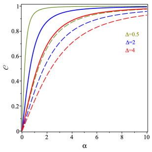
Figure 3: The concurrence $\mathcal{C}$ as a function of $\alpha$, for fixed $t=0.1$ (solid curves) and $t=2$ (dashed curves) at zero temperature. Here we choose $\Delta=0.5$ (green curve), $\Delta=2$ (red curve) and $\Delta=4$ (blue curve).

IV.2 Thermal Quantum Coherence

Firstly, we study how the concurrence $\mathcal{C}$ is affected by temperature $T$. In Fig. 4 we depict the concurrence $\mathcal{C}$ as a function of the temperature $T$ in the logarithmic scale and for different values of the Rashba coupling $\alpha$, with $\Delta=2$ and $t=1$. It is clear to see that there are two different regimes: the first one corresponds to a strong Rashba coupling $\alpha=10$ (blue curve), where we can see the concurrence for $T=0$ becomes $\mathcal{C}\approx 0.98$. It is also observed that the concurrence monotonously leads to zero at the threshold temperature $T_{th}\approx 4.558$. For $\alpha=2$ (green curve), the concurrence $(\mathcal{C}\approx\frac{1}{\sqrt{2}})$ is smaller than to the previous case at low temperature. However, it decreases quickly as temperature raise and finally vanishes at threshold temperature $T_{th}\approx 1.728$. The second one corresponds to weak Rashba coupling strength, e.g., $\alpha=1$ (red curve), where we obtain a weak entanglement at zero temperature $\mathcal{C}\approx 0.447$, which remains almost constant at low temperature. Then, the concurrence monotonically decreases with increasing temperature until it completely vanishes at the threshold temperature $T_{th}\approx 1.224$. This result shows that $\alpha$ can be used for either tuning on or off the entanglement.

In Fig. 5(a), we illustrate the density plot of concurrence $\mathcal{C}$ as a function of $T$ and $t$, for fixed values of $\Delta=2$ and $\alpha=1$. The blue color corresponds to the entangled region, while the white color corresponds to the unentangled region. One interesting feature observed here is that the system is strongly entangled around $t=0$ and at low temperatures. There is a threshold temperature above which the entanglement becomes zero. We also observed that the concurrence gradually decreases with the increase of the tunnel effect parameter, which indicates that the tunnel effects weakens the quantum entanglement. Furthermore, a similar density plot for the concurrence is reported in Fig. 5(b) as a function of $T$ and $\Delta$ for fixed values of $t=0.5$ and $\alpha=1$. Still, in the same panel, we can notice that when the Zeeman splitting is null, the model is weakly entangled in a low temperature region. But quickly, the concurrence disappears due to the thermal fluctuations as the temperature increases. Additionally, the density plot also shows that the entanglement is strong for weak Zeeman splitting values at zero temperature, but the entanglement decreases as the Zeeman parameter increases. On the other hand, when $T$ increases, the concurrence $\mathcal{C}$ decreases rapidly until achieving the threshold temperature, above which the thermal entanglement becomes null.

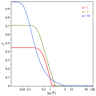
Figure 4: The concurrence $\mathcal{C}$ as a function of temperature $T$ in the logarithmic scale, for fixed $\Delta=2$, $t=1$. Here, $\alpha=1$ (red curve), $\alpha=2$ (green curve), $\alpha=10$ (blue curve).

In Fig. 6, the thermal effects on populations $\rho_{11}$ (red curve), $\rho_{22}$ (green curve) and concurrence (black curve), are reported for two values of the Rashba coupling. In this figure, the blue dashed line shows the threshold temperature going from the region of constant concurrence to the region where concurrence monotonously decreases as the temperature increases, this threshold temperature also describes the beginning of population change. In Fig. 6(a) for the Rashba coupling $\alpha=0.1$. We have observed that for low temperatures, the population and concurrence remain constant in a small range of temperature, in this region we find that the populations are $\rho_{11}\approx 0.003$ (red curve) and $\rho_{22}\approx 0.4996$ (green curve). These results suggest that the weakly entangled qubits are in the ground state $\left|\varphi_{2}\right>\approx-0.017i\left(\left|L0\right>+\left|R0\right>\right)-0.7068\left(-\left|L1\right>+\left|R1\right>\right)$ for low temperature regimes, so the concurrence is $\mathcal{C}\approx 0.0499$. In this figure, the blue dashed line shows the threshold temperature is $T_{th}\approx 0.1777$. Thus, we found that quantum entanglement is sensitive to population change as a consequence of increasing temperature. On the other hand, in Fig.6(b) for a strong Rashba coupling $\alpha=10$, we observe a sudden increase of $\rho_{11}$ which attains the value $\rho_{11}\approx 0.2$ (red curve), a decrease for $\rho_{22}\approx 0.3$ (green curve) and the concurrence reaches the value $\mathcal{C}\approx 0.9805$ at low temperatures, this concurrence is constant until the threshold temperature $T_{th}\approx 0.0191$, see the blue dashed line. Therefore, due to thermal fluctuations, the populations undergo a change and concurrence decreases until it disappears. In any case, with increasing temperature regardless of the value of the Rashba coupling, the population corresponding to the $\rho_{11}$ state increases, while the population $\rho_{22}$ decreases until at higher temperature the eigenstates are distributed equally, reaching the value $0.25$.

In Fig.7, we plot the fidelity $F$ between the ground state $\left|\varphi_{2}\right>$ and the thermal state $\rho_{AB}(T)$ as a function of temperature $T$ in the logarithmic scale. We can see that the mixed-state fidelity approaches ground-state fidelity i.e. $F=1$, when the temperature leads to zero. On the other hand, when the temperature increases the ground state mixes with the excited states, allowing the fidelity to decrease monotonically as the temperature increases. It is also observed that for $T=0$, the figure exhibits the change of the fidelity $F=0.5$ (red curve), since the ground states become the degenerate states $\left|\varphi_{2}\right>$ and $\left|\varphi_{4}\right>$ for fixed tunneling parameter $t=0$.

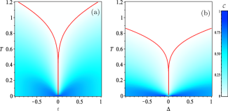
Figure 5: The density plot of the thermal concurrence $\mathcal{C}$. a) as a function of $T$ versus $t$ with $\Delta=2$ and $\alpha=1$. b) as a function of $T$ versus $\Delta$ with $t=0.5$ and $\alpha=1$. In these figures, red solid curve is the contour between the entangled region (blue) and the disentangled region (white).

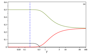
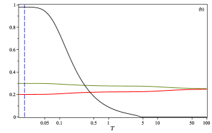
Figure 6: The thermal effects on the population $\rho$ and concurrence $\mathcal{C}$. Here, the red curve corresponding to $\rho_{11}$ and green curve corresponding to $\rho_{22}$, while black curve represents to $\mathcal{C}$. The parameters are set as $\Delta=2$, $t=1$. (a) $\alpha=0.1$, (b) $\alpha=10$.

Finally, in Fig. 8, we give the plot of correlated coherence and the concurrence as a function of temperature at a fixed value of the tunneling parameter $t=1$, Rashba coupling $\alpha=10$, Zeeman parameter $\Delta=2,$ and for different values of the parameter $\theta$. Note that in these figures, we include the curves of total quantum coherence $\mathcal{C}_{l_{1}}(\rho_{AB})$ (black curve) and the local quantum coherence $\mathcal{C}_{l_{1}}(\rho_{A})+\mathcal{C}_{l_{1}}(\rho_{B})$ (black dashed curve) for a better understanding of these amounts. In Fig. 8(a), we plot the correlated coherence and the concurrence as a function of temperature $T$, in the basis of the eigenenergies which corresponds to the angle $\theta=0$ and to $\varphi=0$ in the transformation $U$(see Eq. 14). These curves show that, for $T\rightarrow 0$, the correlated coherence $\mathcal{C}_{cc}$ (solid blue curve) is higher than the thermal entanglement $\mathcal{C}$(solid red curve). The difference between them is the untangled quantum correlation (quantum discord). We can also notice the presence of a plateau in the correlated coherence in this low temperature regime, this is due to the fact that the correlated coherence of the ground state $(\left|\varphi_{2}\right>)$ is weak affected by thermal fluctuations in this regime. From this figure, it is also easy to see that, as the temperature increases, the entanglement (red curve) decays up to threshold temperature $T_{th}\approx 4.5$, while the total quantum coherence gradually decreases as the temperature increases. In Fig. 8(b), we repeat the analysis for a starting angle of $\theta=\frac{\pi}{8}$. Here, we observed a decrease in local quantum coherence that accompanies the lowering of total quantum coherence, which follows as a consequence of the reduction of correlated coherence. Interestingly, the behavior of correlated coherence, as well as total and local quantum coherence qualitatively follows the same pattern as in Fig. 8(a). In Fig. 8(c), we choose $\theta$ close to $\frac{\pi}{4}$, $\left(\theta=0.95\frac{\pi}{4}\right)$ and $\varphi=0$, for this choice of the $\theta$ parameters, we observed a dramatic decrease in correlated coherence. In addition, we can see that the local quantum coherence (dashed black curve) is almost null. Then, it can be seen that the correlated coherence almost entirely constitute the total quantum coherence (solid black curve) for this particular choice of $\theta$. On the other hand, for high temperatures and after the concurrence and the local coherence have disappeared, the total quantum coherence is composed solely of non-entangled quantum correlations.

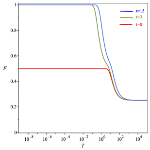
Figure 7: The thermal fidelity $F$ as a function of temperature. Here, the red curve corresponding to tunneling coupling $t=0$, green curve corresponding to $t=3$, while blue curve represents the case $t=15$. The parameters are set as $\Delta=2$, $\alpha=10.0$

To recover the independence of the correlated coherence basis, we choose the local natural basis of $\rho_{A}$, which is obtained by choosing $\theta=\frac{\pi}{4}$ and $\varphi=0$ (the reduced density matrix $\rho_{B}$ is already diagonal). Thus, in Fig. 8(d), the concurrence and quantum coherence are analyzed for the incoherent basis $\theta=\frac{\pi}{4}$ and $\varphi=0$. It is interesting to note that at low temperatures, the entangled quantum correlations of the system are stored entirely in the quantum coherence; this indicates that, in this case, the correlated coherence captures all the thermal entanglement information. As the temperature increases, the thermal fluctuations generate a slight increase in quantum coherence, while the entanglement decays and disappears at the threshold temperature, $T\approx 4.5$. Finally, the correlated coherence leads monotonically to zero.

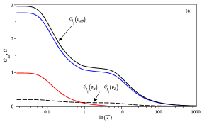
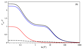
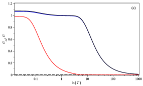
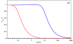
Figure 8: Correlated coherence $\mathcal{C}_{cc}$ (blue solid curve) and concurrence $\mathcal{C}$ (red solid curve) versus $T$ in the logarithmic scale for different values of $\theta$. In particular we set $\Delta=2$, $t=1$, $\alpha=10$ and $\varphi=0$. (a) $\theta=0$, (b) $\theta=(\frac{\pi}{8})$, (c) $\theta=0.95(\pi/4)$, (d) $\theta=(\pi/4)$.

V Conclusions

This paper considers a device composed of a single electron in a double quantum dot subjected to a homogeneous magnetic field and a spin-flip tunnel coupling due to the Rashba spin-orbit interaction in a thermal bath. The proposed model was exactly solved and the effects of temperature on quantum coherence were analyzed. Firstly, the spectrum energy is discussed. It is shown that the tunneling parameter contributes to breaking the energy degeneracy, while the Rashba coupling induces anti-crossing phenomena in the electron energy spectrum. In this model, we have investigated the thermal entanglement and correlated coherence. We show that thermal entanglement for a single electron is possible via charge and spin qubits in a silicon double quantum dot. Furthermore, our results suggest that the Rashba parameter turns on the thermal entanglement and be tuned conveniently. We also have investigated the influence of the Rashba coupling on the population and concurrence. These results show that are sensitive to temperature and Rashba coupling, particularly, in the regime of low temperatures, the concurrence and populations form plateaus. However, with increasing temperature, the populations undergo changes in their behavior, while the concurrence decreases, this is a consequence of thermal fluctuations. Additionally, we present an analysis of the thermal fidelity between the fundamental state and the thermal states, and we showed that the fidelity is maximum for low temperatures, while, with increasing temperature, the fidelity decreases monotonically due to the mixture between the ground state and the excited states. Moreover, we found a direct connection between entanglement and quantum coherence. We ultimately compare the concurrence with correlated coherence, which is responsible for quantum correlations. Quantum coherence is a base-dependent concept. We have choosen an incoherent basis for the local coherence ($\theta=\frac{\pi}{4}$, $\varphi=0$), obtaining the correlated coherence. In particular, we reported that the correlated coherence measure is equal to the concurrence for low temperatures. The thermal entanglement must then be viewed as a particular case of quantum coherence. Furthermore, the model showed a peculiar thermally-induced increase of correlated coherence due to the emergence of non-entangled quantum correlations as the entanglement decreased. When $T$ is high enough, the quantum entanglement disappears as thermal fluctuation dominates the system. Overall, our results highlight that the Rashba coupling can be used successfully to enhance the thermal performance of quantum entanglement. Then, we can safely conclude that quantum coherence is more robust than entanglement under the effect of a thermal bath. The results also suggest that correlated coherence may potentially be a more accessible quantum resource in comparison to entanglement, and that this is something worth investigating in future work.

VI Acknowledgments

This work was partially supported by CNPq, CAPES and Fapemig. Moises Rojas would like to thank National Council for Scientific and Technological Development (CNPq) - Grant No. 317324/2021-7.

References

- (1) E. Chitambar, G. Gour, Rev. Mod. Phys. 91, 025001 (2019).
- (2) A. Streltsov, G. Adesso, M. B. Plenio, Rev. Mod. Phys. 89, 041003 (2017).
- (3) C. H. Bennett, D. P. DiVincenzo, Nature 404, 247 (2000).
- (4) C. H. Bennett, H. J. Bernstein , Phys. Rev. A 53, 2046 (1996).
- (5) L. Amico, R. Fazio, A. Osterloh and V. Vedral, Rev. Mod. Phys. 80, 517 (2008).
- (6) F. Frwis, W. Dr, Phys. Rev. Lett. 106, 110402 (2011).
- (7) V. Giovannetti, S. Lloyd, L. Maccone, Science 306, 1330 (2004).
- (8) F. G. S. L. Brandão, M. Horodecki, J. Oppennheim, J. M. Renes, R. W. Spekkens, Phys. Rev. Lett. 111, 250404 (2013); M. Lostaglio, D. Jennings, T. Rudolph, Nat. Commun. 6, 6383 (2015).
- (9) J. P. Santos, L. C. Céleri, G. T. Landi, M. Paternostro, Nat. Quant. Inf. 5, 23 (2019).
- (10) C. M. Li, N. Lambert, Y. N. Chen, F. Nori, Sci. Rep. 2, 885 (2012).
- (11) M. C. Arnesen, C. Bose, V. Vedral, Phys. Rev. Lett. 87, 017901 (2001).
- (12) G. L. Kamta, A. F. Starace, Phys. Rev. Lett. 88, 107901 (2002).
- (13) M. Rojas, S. M. de Souza, O. Rojas, Ann. Phys. 377, 506 (2017).
- (14) M. Freitas, C. Filgueiras, M. Rojas, Ann. Phys. (Berlin) 531, 1900261 (2019).
- (15) Q. A. Turchette, C. S. Wood, B. E. King, C. J. Myatt, D. Leibfried, M. W. Itano, C. Monroe, D. J. Wineland, Phys. Rev. Lett. 81, 3631 (1998).
- (16) J. M. Raimond, M. Brune, S. Haroche, Rev. Mod. Phys. 73, 565 (2001).
- (17) L. Davidovich, et. al., Phys. Rev. A 50, R895 (1994).
- (18) J. R. Petta, A. C. Johnson, J. M. Taylor, E. A. Laird, A. Yacoby, M. D. Lukin, C. M. Marcus, M. P. Hanson, A. C. Gossard, Science, 309, 2180 (2005).
- (19) G. Shinkai, T. Hayashi, T. Ota, T. Fujisawa, Phys. Rev. Lett. 103, 056802 (2009); T. Fujisawa, T. Hayashi, Y. Hirayama, J. Vac. Sci. Technol. B 22, 2035 (2004).
- (20) J. Gorman, D. G. Hasko, D. A. Williams, Phys. Rev. Letts. 95, 090502 (2005).
- (21) M. Benito, X. Mi, J. M. Taylor, J. R. Petta, Guido Burkard, Phys. Rev. B, 96, 235434 (2017).
- (22) D. Loss, D. P. DiVincenzo, Phys. Rev. A 57, 120 (1998).
- (23) B. D’Anjou, G. Burkard, Phys. Rev. B 100, 245427 (2019).
- (24) J. Mielke, J. R. Petta, G. Burkard, Phys. Rev. X Quantum 2, 020347 (2021).
- (25) Y. -C. Yang, S. N. Coppersmith, M. Friesen, Phys. Rev. A 101, 012338 (2020).
- (26) T. Itakura, Y. Tokura, Phys. Rev. B 67, 195320 (2003).
- (27) M. Urdampilleta, A. Chatterjee, Ch. Ch. Lo, T. Kobayashi, J. Mansir, S. Barraud, A. C. Betz, S. Rogge, M. F. Gonzalez-Zalba, J. J. L. Morton, Phys. Rev. X 5, 031024 (2015).
- (28) P. A. Oliveira, L. Sanz, Annl. Phys. 356, 244 (2015).
- (29) B. Szafran, Phys. Rev. B 101, 075306 (2020).
- (30) F. F. Fanchini, L. K. Castelano, A. O. Caldeira, New. J. Phys. 12, 073009 (2010).
- (31) Xiao-Ke Qin, Europhys. Lett. 114, 37006 (2016).
- (32) H. S. Borges, L. Sanz, J. M. Villas-Bôas, O. O. Diniz Neto, A. M. Alcalde, Phys. Rev. A 85, 115425 (2012).
- (33) F. M. Souza, P. A. Oliveira, L. Sanz, Phys. Rev. A 100, 042309 (2019).
- (34) K. W. Choo, L. C. Kwek, Phys. Rev. B, 75, 205321 (2007); F. D. Pasquale, G. Georgi, S. Pagonelli, Phys. Rev. Lett, 93, 120502 (2004).
- (35) A. Purkayastha, G. Guarnieri, M. T. Mitchison, R. Filip, J. Goold, npj Quantum Inf., 6, 27 (2020).
- (36) D. D. B. Rao, S. Gosh, P. K. Panigrahi, Phys. Rev. A 78, 042328 (2008).
- (37) C. Filgueiras, O. Rojas, M. Rojas, Ann. Phys. (Berlin) 532, 2000207 (2020).
- (38) J. L. D. de Oliveira, M. Rojas, C. Filgueiras, Phys. Rev. E 104, 014149 (2021).
- (39) F. N. M. Froning, L. C. Camenzind, O. A. H. van der Molen, A. Li, E. P. A. M. Bakkers, D. M. Zumbuhl, F. R. Braakman, Nat. Tech. 16, 308 (2021).
- (40) N. W. Hendrickx, W. I. L. Lawrie, L. Petit, A. Sammak, G. Scappucci, M. Veldhorst, Nat. Commun. 11, 3478 (2020).
- (41) Y. A. Bychkov, E. I. Rashba, J. Phys. C 17, 6039 (1984).
- (42) G. Dresselhaus, Phys. Rev. 100, 580 (1955).
- (43) L. Chotorlishvili, A. Gudyma, J. Watzel, A. Ernst, J. Berakdar, Phys. Rev. B 100, 174413 (2019).
- (44) Y-Ch. Li, X. Chen, J. G. Muga, E. Y. Sherman, New J. Phys. 20, 113029 (2018).
- (45) F. Ginzel, A. R. Mills, J. R. Petta, G. Burkard, Phys. Rev. B 102, 195418 (2020).
- (46) T. Baumgratz, M. Cramer, M. B. Plenio, Phys. Rev. Lett. 113, 140401 (2014).
- (47) M. L. Hu, X. Hu, J. C. Wang, Y. Peng, Y. R. Zhang, H. Fan, Phys. Rep. 762, 1 (2018).
- (48) A. Streltsov, U. Singh, H. S. Dhar, M. N. Bera, G. Adesso, Phys. Rev. Lett. 115, 020403 (2015).
- (49) K. C. Tan, H. Kwon, C-Y. Park, H. Jeong, Phys. Rev. A 94, 022329 (2016).
- (50) T. Kraft, M. Piani, J. Phys. A: Math. Theor. 51, 414013 (2018).
- (51) H. Ollivier, W. H. Zurek, Phys. Rev. Lett. 88, 017901 (2001); D. Girolami, G. Adesso, Phys. Rev. A,83, 052108 (2011).
- (52) T. Werlang, G. Rigolin, Phys. Rev. A 81, 044101 (2010).
- (53) X. -L. Wang, Q. -L. Yue, Ch. -H. Yu, F. Gao, S. -J. Qin, Sci. Rep. 7, 12122 (2017).
- (54) J. Ma, B. Yadin, D. Girolami, V. Vedral, M. Gu, Phys. Rev. Letts. 116, 160407 (2016).
- (55) W. K. Wootters, Phys. Rev. Lett. 80, 2245 (1998).
- (56) S. Hill, W. K. Wootters, Phys. Rev. Lett. 78, 5022 (1997).
- (57) D. C. Li, Z. L. Cao, Eur. Phys. J. D 50, 207 (2008).
- (58) R. Jozsa, J. Mod. Opt. 41, 2315 (1994).
- (59) Y. Zhou, G. F. Zhang, S. S. Li, A. Abliz, Europhys. Lett. 86, 50004 (2009).
- (60) F. Borjans, D. M. Zajac, T. M. Hazard, J. R. Petta, Phys. Rev. Appl. 11, 044063 (2019).
- (61) A. Hollmann, T. Struck, V. Langrock, A. Schmidbauer, F. Schauer, T. Leonhardt, K. Sawano, H. Riemann, N. V. Abrosimov, D. Bougeard, L. R. Schreiber, Phys. Rev. Appl. 13, 034068 (2020).